Shlomo Reutlinger

Techniquesfor Project Appraisalunder Uncertainty

, r, -wn OC P-1 0

~~~ _

SLC001997b- -_-WORLD BANK STAFF OCCASIONAL PAPERS IEE NUMBER TEN

Pub

lic D

iscl

osur

e A

utho

rized

Pub

lic D

iscl

osur

e A

utho

rized

Pub

lic D

iscl

osur

e A

utho

rized

Pub

lic D

iscl

osur

e A

utho

rized

Pub

lic D

iscl

osur

e A

utho

rized

Pub

lic D

iscl

osur

e A

utho

rized

Pub

lic D

iscl

osur

e A

utho

rized

Pub

lic D

iscl

osur

e A

utho

rized

World Bank Staff Occasional Papers

No. 1. Herman G. van der Tak, The Economic Choice between Hydroelectricand Thermal Power Developments.

No. 2. Jan de Weille, Quantification of Road User Savings.No. 3. Barend A de Vries, The Export Experience of Developing Countries

(out of print).No. 4. Hans A. Adler, Sector and Project Planning in Transportation.No. 5. A. A. Walters, The Economics of Road User Charges.No. 6. Benjamin B. King, Notes on the Mechanics of Growth and Debt.No. 7. Herman G van der Tak and Jan de Wezlle, Reappraisal of a Road Project

in Iran.No. 8. Jack Baranson, Automotive Industries in Developing CountriesNo. 9. Ayhan ,ilingiroglu, Manufacture of Heavy Electrical Equipment in

Developing Countries.No. 10. Shlomo Reutlinger, Techniques for Project Appraisal under Uncertainty.No. ll. Louis r. Pouliquen, Risk Analysis in Project Appraisal.No. 12 George C. Zatdan, The Costs and Benefits of Family Planning Programs.No 13 Herman G. van der Tak and Anandarup Ray, The Economic Benefits of

Road Transport Projects (out of print).No. 14. Hans Heinrich Thias and Martin Carnoy, Cost-Benefit Analysis in

Education A Case Study of Kenya.No. 15. Anthony Churchill, Road User Charges in Central America.No. 16. Deepak Lal, Methods of Project Analysis A Review.No. 17. Kenji Takeuchi, Tropical Hardwood Trade in the Asia-Pacific Region.No. 18. Jean-Pierre Jallade, Public Expenditures on Education and Income

Distribution in ColombiaNo. 19. Enzo R. Grillt, The Future for Hard Fibers and Competition from

SyntheticsNo. 20. Alvin C. Egbert and Hyung M. Kim, A Development Model for the

Agricultural Sector of Portugal.No. 21. Manuel Zymelman, The Economic Evaluation of Vocational Training

Programs.No. 22. Shamsher Singh and others, Coffee, Tea, aid Cocoa: Market Prospects

and Development LendingNo. 23 Shlomo Reutlinger and Marcelo Selowsky, Malnutrition and Poverty:

Magnitude and Policy Options.No. 24. Syamaprasad Gupta, A Model for Income Distribution, Employment,

and Growth- A Case Study of Indonesia.No. 25. Rakesh Mohan, Urban Economic and Planning Models.No. 26. Susan Hzll Cochrane, Fertility and Education: What Do We Really

Know?No. 27. Howard N. Barnum and Lyn Squire, A Model of an Agricultural House-

hold: Theory and Evidence.

WORLD BANK STAFF OCCASIONAL PAPERS NUMBER TEN

The views and interpretations in this paper are those of the authors,

who are also responsible for its accuracy and completeness. They

should not be attributed to the World Bank, to its affiliated

organizations, or to any individual acting in their behalf.

WORLD BANK STAFF OCCASIONAL PAPERS NUMBER TEN

SHLOMO REUTLINGER

TECHNIQUES FORPROJECT APPRAISAL

UNDER UNCERTAINTY

V,co,~1 RIJCTIJ- NDDO OMN

FE 2 498

Published for the World Bank byTHE JOHNS HOPKINS UNIVERSITY PRESS

Baltimore and London

Copyright © 1970by the International Bank for Reconstruction and Development1818 H Street, N.W., Washington, D.C. 20433 U.S.A.All rights reservedManufactured in the United States of America

The Johns Hopkins University Press, Baltimore, Maryland 21218The Johns Hopkins Press Ltd., London

Library of Congress Catalog Card Number 74-94827

ISBN 0-8018-1154-6

Originally published, 1970Second printing, 1972Third printing, 1976Fourth printing, 1979

FOREWORD

I would like to explain why the World Bank does research wvork and whythis research is published. We feel an obligation to look beyond the projectsthat we help to finance toward the whole resource allocation of an economy andthe effectiveness of the use of those resources. Our major concerni, in dealingswith member countries, is that all scarce resources-including capital, skilledlabor, enterprise, and know-how-should be used to their best advantage. Wewant to see policies that encourage appropriate increases in the supply of savings,whether domestic or international. Finally, we are required by our Articles, aswell as by inclination, to use objective economic criteria in all our judgments.

These are our preoccupations, and these, one way or another, are the subjectsof most of our research work. Clearly, they are also the proper concern of any-one who is interested in promoting development, and so we seek to make ourresearch papers widely available. In doing so, we have to take the risk of beingmisunderstood. Although these studies are published by the Bank, the viewsexpressed and the methods explored should not necessarily be consideredl torepresent the Bank's views or policies. Rather, they are offered as a modest con-tribution to the great discussion on how to advance the economic developmentof the uniderdeveloped world.

ROBERT S. McNAMAARA

PresidentThe World Bank

v

TABLE OF CONTENTS

FOREWORD v

PREFACE xi

PART I. PROBABILITY ANALYSIS

I. INTRODUCTION 1

II. ASSESSMENT OF UNCERTAIN EVENTS 7

Formulation of Anticipations 7The Probabilistic Formulation 8A Probabilistic Formulation Facilitates Aggregation 9A Probabilistic Approach Utilizes More Information 11A Probabilistic Formulation Can be Subjected to Meaningful

Empirical Test 12Estimation of Probability Distributions 12

III. PROBABILITY APPRAISAL OF PROJECT RETURNSUNDER UNCERTAINTY 14

General Outline 14The Aggregation Problem 15Illustration of Alternative Procedures for Aggregating

Probability Distributions 18

vii

Discussion of Alternative Estimating Procedures 21

Conceptual Problems Related to Probability Appraisal 24

Biased Estimates 25

Correlation 28Specific Uncertainty Problems in Project Appraisal 31

Uncertainty About Annual Net Benefits 31Equal Annual Correlated and Uncorrelated Benefits 32

Annual Benefits Contain an Uncertain Trend 36

Life of Project 39Estimating Probability Distributions of Annual Benefits 40

Summary and Conclusions on Aggregation of ProbabilityDistributions 41

IV. PROJECT DECISIONS UNDER UNCERTAINTY 44

Introduction 44A Hypothetical Example of the Decision Problem 45

Project Appraisal and Utility Theory 47

Public Investment Decisions 51Selected Decision Problems 54

Value of Information 54

Alternative Project Strategies 56

Time Related Problems 57

PART II. CASE ILLUSTRATIONS

V. CONSTRUCTION OF APPRAISAL MODELS ANDTHEIR DEPLOYMENT 63

Model Construction 63

Deployment of Formal Models 66

Sensitivity Analysis 67

Risk Appraisal 67

Feasibility Appraisal with General Models 68

Ex-Post Evaluation 68

VI. CASE ILLUSTRATION-A HIGHWAY PROJECT 69

The Model 69

Sensitivity Analysis 72AMdvantage of a Postponement 72

The Value of More Information 72Variables Beyond Our Control 74

Probability Distribution of Rate of Return 75

viii

VII. CASE ILLUSTRATION-A HYPOTHETICALIRRIGATION PROJECT 82

Probability Distribution of the Inputs 83Conventional Appraisal of Present Value of Benefits 84Appraisal by Probability Analysis 84

ANNEXREVIEW OF SOME BASIC CONCEPTS AND RULES

FROM PROBABILITY CALCULUS WITH SPECIFICAPPLICATION 87

BIBLIOGRAPHY 94

TABLES1. Probability Distributions of Revenue (X) and Investment

Cost (Y) 182. Probability Distributions of Present Value (R) 193. Cumulative Probability Distribution of R 214. Ratio of Coefficient of Variation of Present Value (CR) to

Coefficient of Variation of Successively UncorrelatedAnnual Benefits (CB) 33

5. Hypothetical Data for Calculating a Variance of thePresent Value when Benefits from Successive Years areUncorrelated or Perfectly Correlated 34

6. Elasticity of Variance of Present Value of a Stream ofBenefits with Respect to Variance of SuccessivelyUncorrelated Benefits (when Bt = B + el) 35

7. Elasticity of the Mean Present Value (R) with Respect toMean Growth (b) and Mean Initial Benefits (A) 37

8. Elasticities of the Variance of Present Value V(R) withRespect to V(b), V(Ro) and V(e) 39

9. Highway Project Benefits and Costs, Single Valued Estimates 7310. Probability Distribution of Initial Traffic Levels and

Corresponding Present Value of Project Net Benefits 7411. Road Project Appraisal Model 7812. Input Data for Road Project Appraisal 8013. The Model 8314. Probability of Various Outcomes of Events 83

FIGURES1. Cumulative Probability Distributions of Present Value 22

ix

2. Illustration of Bias when Yield is Calculated as a Functionof Average Rainfall 27

3. Probability Distribution of Present Value, R 54

4. Probability Distributions of Present Value for AlternativeProject Strategies 56

5. Flow Chart for Road Project Appraisal 71

6. Graphic Illustration of Types of Probability Distributions

Used in Appraisal of Highway Project 76

7. Cumulative Probability Distribution of Rate of Return 77

8. Simulated Probability Distribution of Present Value 84

9. Simulated Probability Distribution of Internal Rateof Return 85

ANNEX TABLES

1. Mean of Present Value, by Year and Interest Rate 92

2. Variance of Present Value, by Year and Interest Rate 93

x

PREFACE

This study is concerned with the appraisal of events which have uncertainoutcomes. This issue is generally recognized, but is usually not explicitlyconsidered in otherwise detailed cost-benefit analysis of investment projects.Application of contingency allowances and sensitivity analyses have beenused as partial remedies. However, for the most part, project benefits arestill estimated and reported in terms of one single outcome which does nottake account of, or record, valuable information about the extent of un-certainty of project-related events.

This paper recommends that the best available judgments about thevarious factors underlying the cost and benefit estimates of the projectbe recorded in terms of probability distributions and that these distribu-tions be aggregated in a mathematically correct manner to yield a probabil-ity distribution of the rate of return, or net present worth, of the project.This procedure in no way eliminates the problem of making judgmentsabout events and relationships in the face of limited and incomplete in-formation, nor does it suggest a unique and simple formula for choosingamong projects or project strategies with varying degrees of riskiness. How-ever, this type of analysis would ensure and encourage that available infor-mation about events affecting the outcome of the project would be morefully utilized and correctly transformed into information about uncertainproject results. Project-related decisions could be made more easily and

xi

more intelligently if returns on projects were reported not in terms of asingle rate, or a wide range of possible returns with undefined likelihoodsof occurrence, but in terms of a probability distribution.

The present paper should be viewed primarily as providing a conceptualframework for further study into the scope and limitations of practicalapplication of probability appraisal and pursuant project decisions. Severalcase studies are currently being investigated in the Bank by Louis Pouliquenand Tariq Husain. The author has benefited from many discussions withthem. The author also wishes to acknowledge helpful comments by HermanG. van der Tak and Jan de Weille of the Sector and Project Group in theEconomics Department and written comments on an earlier draft of thispaper by Bank staff members: Messrs. B. Balassa, L. Goreux, A. Kundu,M. Schrenk, A. E. Tiemann, D. J. Wood of the Economics Department;and D. S. Ballantine, I. T. Friedgut, V. W. Hogg, P. 0. Malone, H. P.Muth, M. Palein, S. Y. Park, M. Piccagli, L. Pouliquen, A. P. Pusar,V. Rajagopalan, S. Takahashi, V. Wouters of the Projects Department.However, the views expressed in this paper are those of the author, and healone is responsible for them.

A. M. KAMARCK

DirectorEconomics Department

xii

PART I

PROBABILITY ANALYSIS

I

INTRODUCTION

The primary purpose of this study is to present a feasible method for

evaluating the riskiness of investment projects. A second objective is to

show how quantitative evaluations of the riskiness of projects might beused in various decision problems. Throughout, the emphasis is on meth-odology and problems of measurement, not on description of various kindsof uncertainty problems, nor is much attention paid to theories which haveno immediate applicability to project appraisal. Uncertainty is every-where, as anyone knows; hence, a general descriptive study of uncertaintyis unnecessary and the specific sources of uncertainty must be identified

for each specific case. In general, however, the uncertainty conditionsrelevant for this study are those unique to a particular project, and not to"global" uncertainties which affect the outcomes of all projects within acountry.

This study does not recommend a specific "best" attitude for a publicinvestment authority or an international lending agency with respect toundertaking projects with uncertain outcomes. To do so, would be aspresumptuous as to advise a government on the income distribution or thecomposition of goods and services it should promote for internal consump-tion. The pursuit of economic development is clearly inconsistent with apolicy of avoiding all risks (there simply are no worthwhile projects withoutrisks). At the other extreme, most people would agree that a project which

1

has a reasonably high probability of turning out badly should not be under-taken if that outcome would mean a considerable deterioration of thepresent economic well-being of a country. However, between those twoextreme choices lie many alternatives whose desirability would depend onthe subjective preferences or aversions to risk of the decision makers andtheir constituents.

This study deals at length with the question of how to evaluate and pre-sent in summary form a measure of the relative riskiness of projects, on thegeneral assumption that a "good" judgment of risk is an important in-gredient for reaching a "best" decision. For all practical purposes, decisionsinvolving choices among uncertain economic returns from investment haveone thing in common: they ask for judgments about the likelihood of themeasure of returns used in the evaluation. For some the most relevantmeasure of returns is "the most likely one" (the mode). Others use exclu-sively a conservative estimate, that is one which has a "high chance ofbeing exceeded," and still others wish to consider an entire set of returns,and their respective likelihoods.1

No attempt is made in this study to present a comprehensive review ofall decision theories dealing with uncertainty. Such comprehensive reviewsare available elsewhere. 2 They are useful to students and research workersbut more often than not they leave the practitioner's problem unresolved.Only a small set of uncertainty hypotheses and decision criteria are pre-sented in this paper.3 They reflect, in the judgment of the author, the most

I Or as Marshak has stated it: "Instead of assuming an individual who thinks heknows the future events, we assume an individual who thinks he knows the prob-abilities of future events. We may call this situation the situation of a game ofchance, and consider it as a better although still incomplete approximation toreality than the usual assumption that people believe themselves to be prophets."(J. Marshak, "Money and the Theory of Assets," Econometrica, 1938).

2 See, for example: K. J. Arrow, "Alternative Approaches to the Theory ofChoice in Risk-Taking Situations," Econometrica, 19:404-437 (1951); M. Friedmanand L. T. Savage, "The Utility Analysis of Choice Involving Risk," Journal ofPolitical Economy, LVI (August 194.8); R. Dorfman, "Basic Economic and Tech-nologic Concepts," A. Maas, et al., Design of Water Resource Systems, HarvardUniversity Press, 1962; D. E. Farrar, The Investment Decision Under Uncertainty,Prentice-Hall, 1962.

3 The point of view taken in this study parallels most nearly the way F. Modigli-ani and K. J. Cohen have stated it: ". . . Probably the best available tool at thisstage is the so-called 'expected-utility' theory . . . starting from certain basicpostulates of rational behaviour this theory shows that the information availableto the agent concerning an uncertain event can be represented by a 'subjective'probability distribution and that there exists a (cardinal) utility function such

2

useful and generally correct approaches to a large number of problemsarising in project appraisal.

The commonly accepted procedure in project evaluation calls for thecalculation of the return from each project and for criteria by which tochoose from among different projects on the basis of the estimated returns.4

The essence of the uncertainty problem is simply that many of the variablesaffecting the outcome of a particular plan of action are not controllable bythe planner or decision-maker. 5 Hence project evaluation which takes dueaccount of uncertainty involves (a) judgments about the likelihood ofoccurrence of the non-controllable variables, (b) calculation of a whole setof possible outcomes or returns for each project, and (c) criteria for choosingamong projects on the basis of sets of possible returns from each project.

Chapter II assesses briefly the nature of uncertainty and the kind ofjudgments which are basic ingredients for the decision making process.Particular attention is paid to the notion that the uncertainty which isrelevant for most decisions is best characterized in terms of a decisionagent's subjective beliefs about the likelihoods of occurrence of variousoutcomes of the uncertain event. Such probability distributions may bebased, of course, on more or less evidence and in this sense might be labeledmore or less "objective." 6 While for any given event it may be desirableto marshall more evidence, if this is possible and not too costly, here wepostulate that for reaching a decision it makes little difference whether anevent is "known" in terms of a more subjective or a more objective prob-ability distribution. It would be a sad mistake to subscribe to a decisiontheory which fails to consider variables simply because their outcomes orprobability distributions of outcomes are not known with certainty. Errorsof omission could be more important than errors of commission. Onlyquantifiable "objective" evidence would then be admitted. What mattersis only whether an event has important consequences for a decision, and

that the agent acts as though he were endeavoring to maximise the expected valueof his utility . . ." ("The Significance and Uses of Ex Ante Data," in Expectations,Uncertainty and Business Behavior, edited by M. J. Bowman, New York, SocialScience Research Council, 1958).

4 The criteria are for the most part derived from a deterministic model whichassumes that the exact returns are known.

5 Such non-controllable variables might be prices, incomes, population, size oflabor force and climate. While governments may have some control over some ofthese variables, they are not likely to be interested or to succeed in controllingthem completely.

6 Of course we do postulate that the source of the judgment is an expert actingwithout prejudice and in good faith.

3

not how "objective" or "subjective" the estimate or probability distribu-

tion of its outcome iS.7

Among the various characterizations of uncertainty advocated by differ-

ent theories, the probabilistic approach has been singled out primarily

because this lends itself best to an appraisal of the possible outcomes of a

project which is affected by uncertainties from many different sources. It

is shown how probabilityjudgments about many basic variables and param-

eters affecting the final outcome of a project can be aggregated into an

estimate of the probability distribution of that final outcome. The advan-

tages of "building up" such an estimate are many: (a) it is generally easier

to formulate judgments about the outcomes of basic events than about the

outcomes from a project because such events are frequently recurring,

whereas projects are usually unique in some respect, (b) the outcomes of

events, such as rainfall, production functions or prices are likely to be

evaluated with less emotional bias and more factual evidence than a proj-

ect's overall benefits, (c) judgments about the outcomes of various "simple"

events utilize the experience of many experts who should be in the best

position to know,-and, finally, (d) analytical insights into the desirability

of restructuring a project can be gained from knowledge of the specific

contribution of each underlying factor to the probability distribution of

the project's final outcome.The "subjective" definition of probability implies at once that the

process of estimation is both an art and a science. The quality of judgments

involved in estimation will vary with the nature of the variables and the

appraiser's expertise in interpolating and extrapolating related observa-

tions and experience. Quite generally, desirable prerequisites for good judg-

ments are (a) knowledge of past outcomes of the event (experience and

data), (b) knowledge of basic relationships which could explain why the

outcomes of the event might have varied in the past and how they might

vary in the future (a model), and (c) sound procedures for interpreting the

interaction of model and data (statistics). To the extent that formal theory,

subject matter expertise, and analytical tools can assist in the estimation

process, they are assumed to be known to project appraisers and are not

elaborated in this study.

7 In the terminology suggested by Frank Knight, events whose probabilitydistributions can be objectively known are sometimes labeled as "risks," and sub-jectively conceived distributions are called "uncertainties." The point of viewtaken in this study is that this is not a meaningful classification, both because thereare no "subjective" but only more or less "objective" estimates, and because theextent of objectivity does not necessarily alter their interpretation in terms ofdecisions. (F. H. Knight, Risk Uncertainty and Profit, Boston, Houghton MifflinCo., 1921.)

4

Chapter III discusses how to aggregate probability distributions ofrelevant factors and parameters into a probability distribution of the eco-nomic returns of a project. The problems arising when uncertain estimatesof the various factors are combined have been for the most part neglectedor inadequately treated by conventional appraisal methods, although forthese aggregation problems at least it is possible to prescribe a uniquelycorrect methodology. The factors one chooses to consider in any economicappraisal of a project, and the prediction of their outcomes and estimationsof how they interrelate are always a matter for subjective judgments withinthe limits described by relevant theory and subject matter expertise. Theorganization's control over these judgments does not extend far beyond itscapacity for hiring able engineers, agronomists, economists, etc., who willcome up with the best possible judgments consistent with the state of thearts. By contrast the aggregation procedures themselves can and shouldbe exactly prescribed in order to transmit as far as possible and as correctlyas possible all the information and judgments made on each of the relevantfactors affecting the costs and benefits from a project.

Probability appraisal or risk analysis as discussed in Chapter III doesnothing more than suggest that the proper probability calculus be used inaggregating probabiliky judgments about the many events influencing thefinal outcome of a project. Just as it is generally accepted that 2 + 2 is 4and not 5, so there are logical, though less generally known, rules for ag-gregating probability distributions of uncertain events. A major reasonwhy these rules have not been more widely used is the complexity andmultitude of calculations which are required in their application. However,present-day availability of high-speed computers makes their applicationnot only desirable but definitely feasible. The only exception to this recom-mendation is the case where even the most pessimistic estimates for allof the variables and parameters affecting a project's net benefits result ina satisfactory measure of the return.8 In this case a probability appraisalmight still satisfy some intellectual curiosity but would be redundant forthe overall project decision. Even in this case, however, one could find ituseful to do probability appraisals if the objective is to investigate alterna-tive ways of implementing the project.

The primary purpose of Chapter III is to illustrate, with some highlystylized and hypothetical streams of costs and benefits, why applicationof the probability calculus to aggregation is important, and to show thesensitivity of the present value of a stream of net benefits to probabilitydistributions and correlations of various basic events. The method of ap-

8 Or conversely, where the most optimistic estimates result in an unsatisfactoryreturn.

proximation by a simulated sample is briefly described, and recommended

for estimation of probability distributions of rates of returns from actual

projects. The simplicity of calculation and the adaptability of this method

to any type of model and conceivable set of probability distributions make

this a preferable method, provided that the resulting distribution is ap-

proximated by an adequate sample. 9 Only under very restrictive assump-

tions about the model and the distributions would it be practical to calcu-

late means and standard deviations of an aggregated variable by using

mathematical methods for aggregation. Mathematical aggregation of

probability distributions may be useful also for partial analyses.

The final crucial phase of project appraisal is, of course, the ranking of

alternative projects, or of courses of action to be taken in a given project.Unfortunately, precise recommendations can be made only on aggregate

procedures. The choice on any alternative courses of action subject to un-

certain outcomes, like the estimate of probability distributions, involves a

large element of subjective judgment. A very large number of decisions

cannot be classified in any objective way as "right" or "wrong" (in an

a priori sense), no matter how utility or preferences are defined. Decisions

involving public projects raise questions about the distribution of benefits

and costs, and many differing preferences with respect to risk have to be

taken into account. Some of these decision problems are discussed in Chap-

ter IV. But while theory cannot suggest a unique general solution to these

problems, it is nevertheless quite apparent that decision-makers do wish

to know the likelihood of outcomes from alternative courses of action in

order to reach decisions. Hence, project appraisals are better if they provide

this information. Furthermore, there are certain limited activities of con-

cern in project appraisal, such as gathering of additional information or

strategies involving sequential decisions, which can be best appraised in a

probabilistic decision framework. Chapter IV presents a brief discussion of

the application of probabilistic information to such decision problems.

Practical procedures and problems in carrying out project evaluations

which take account of uncertainty are reviewed in Part II. Any quantita-

tive evaluation explicitly incorporating uncertainty requires construction

of a mathematical model. In Chapter V it is demonstrated that preparation

of a formal model does not require unusual mathematical skills. Several

uses of such models, particularly when they are programmed for com-

puterized calculations, are discussed. Illustrative applications of the meth-

ods discussed throughout the paper are presented in Chapters VI and VII.

D Probability appraisal by simulation is being applied to several IBRD projects.For case studies and tentative conclusions on methodological aspects, see LouisPouliquen, Risk Analysts in Project Appraisal, a forthcoming World Bank StaffOccasional Paper.

6

II

ASSESSMENT OF UNCERTAIN EVENTS

Millions of dollars have been invested in Project A in anticipation ofgreat benefits to the country. But on hindsight, the benefits have beendisappointing or even inadequate to cover costs. Elsewhere, Project B hashad far better results than anticipated during its planning stage. Shouldprojects like Project A have never been undertaken and the Project Bkind of investment have been expanded? This in a nutshell, is the problemwhich arouses interest in the study of decisions under uncertainty. Clearly,the success of one project and the failure of another is no evidence that awrong decision has been made. They merely give rise to two kinds of ques-tions: were the realized outcomes anticipated, or were they a completesurprise, and, given a "correct" anticipation, was the decision a "correct"one?'

Formulation of Anticipations

First, what is a "correct" anticipation? Does "correct" mean that ananticipation must be confirmed by the realization? Certainly not, if theanticipation in which we are interested is a single outcome.2 It is almost

I The "optimal" decision problem is discussed in Chapter IV.2 If the outcomes of an event are observable many times over and if the decision

pertains to the entire set of outcomes, an anticipation of a frequency distributionof outcomes might be nearly correct in the sense that an anticipation can be expectedto be approximately realized (if the number of observations on which the anticipa-tion is based and the number of realizations is large enough).

7

axiomatic that under uncertainty, no anticipation could be expected to becorrect in this sense. Instead, a "correct" anticipation could be defined asone which is not refuted by a realization. Applying this criterion it isevident that a single valued anticipation of an outcome can hardly qualify.At the other extreme, an anticipation which stretches over the entire rangeof possible realizations will be a "correct" anticipation.

Unfortunately correct anticipations in this objective sense are not neces-sarily satisfactory for reaching decisions, and it is after all primarily for thepurpose of making choices that anticipations are formulated. Correctanticipations in this sense are not even unique.

Consider for instance a statement of anticipation whereby an outcomeis said to be highly likely within a given range and extremely unlikely out-side this range. This anticipation is as "correct" as one which assigns nolikelihoods at all to possible outcomes in the sense that no realizations couldrefute the stated anticipations. Similarly correct is a statement whichassigns numerical values to the relative likelihoods of various outcomes-for instance a 60 percent likelihood that a certain crop yield will be between80 and 100 and a 40 percent likelihood that the yield will be between 100and 120. The choice between alternative formulations of correct anticipa-tions must be sought then on other grounds.

Some seek to distinguish between good and bad formulations of thenature of uncertainty on the basis of relative objectivity in the derivationof the estimate. Clearly, a statement of anticipation which defines possibleoutcomes in terms of specific relative likelihoods is less universally accept-able than one which does not distinguish between likelihoods. Similarly,the likelihoods of outcomes of an event which can be observed many timesover are less disputable than the likelihoods of a non-recurring event. It isnot clear, however, how relevant an objective formulation of anticipationsis for analyzing how investors do act or even ought to act.3

The Probabilistic Formulation

Most decision theories adopt a particular formulation of anticipations onthe basis of how closely it is thought to correspond with the way decision-makers actually think about uncertain outcomes in relation to their deci-

3 Game-theoretic decision models are primarily justified on the basis of theirreliance on the objective formulation of anticipations. But then again it is difficultto see why the objective formulation of the uncertainty condition should be im-portant when the choice criteria or the choice from among many decision modelsis a subjective matter.

8

sions. 4 There is pretty general agreement that the likelihoods of outcomesdo concern decision-makers and that it makes little difference for a decision

whether these likelihoods are judgments based on mere hunches or on an

enormous amount of frequency evidence. Furthermore, since the likelihood'

of outcomes and, to a more limited extent, even the full range of outcomes

generally cannot be objectively determined, it is now commonly accepted

that "the uncertainty of the consequences, which is controlling for be-

haviour, is basically that existing in the mind of the chooser,"5 that is,

the evaluation of risk is subjective.

A Probabilistic Formulation Facilitates Aggregation

A good portion of this paper is devoted to an exposition of how investors

and project appraisers might go about formulating their expectations

about the outcomes from a given investment, say the rate of return or the

discounted present value of net benefits. Any estimate of such an outcome

from an investment usually needs to be developed from information about

the effects of many variables (cost items, production quantities, prices,

etc.) and their values. This is in essence what an investment appraisal is

all about. Similarly, of course, the various outcomes from an investment

under uncertainty conditions arise also from the wide range of values which

relevant non-controllable variables and parameters of the relevant relation-

ships take on as a result of uncertainty. Now, it may be satisfacotry (and"objectively" more correct than formulation of another anticipation) tosay that production, prices and various cost items will fall into specified

ranges. But, to "build" up an estimate of, say, the rate of return, from wide

ranges of the relevant variables and parameters without regard to likeli-hoods, and particularly the likelihoods of compensating events, would lead

to quite unacceptable results.It is easy to see that there is little chance that all the worst, or the best,

4 R. M. Aldeman, "Criteria for Capital Investment," Operational Research

!Ruarterly, March 1965 summarizes the ongoing debate between objectivists andsubjectivists pretty well: "As there are so many subjective elements in the choiceof criterion to use, there seem to be no valid grounds for objecting to subjectiveelements within the criterion. Certainly, it seems that whenever a criterion con-taining subjective elements is proposed there will be cries that it is not objective.Likewise, however, if a criterion that claims objectivity is proposed, there are criesthat it does not take into account the decision maker's subjective valuation of pay-offs involved, nor his subjective beliefs."

5 J. Marshak, "Alternative Approaches to the Theory of Choice in Risk-TakingSituations," Econometrica, Vol. 19, No. 4, October 1951, pp. 404-437.

9

of the anticipations will appear in combination. This is so no matter howdifficult it is to specify the basic probability distributions. The only way,so far, to handle this aggregation problem is to use the probability calculus.It is one thing to believe that one event has as good a chance to turn outfavorably as unfavorably, and another matter to believe that there is asmuch of a chance that luck or misfortune will hold out simultaneously for alarge number of independent events as there is a chance for some turningout favorably and others unfavorably. If it is thought, for instance, thatX, Y and Z are independent events (that is that their outcomes are in noway correlated), then the probability calculus tells us that the probabilityof encountering a combination of the most unfavorable outcomes of allthree events is the product of the probabilities of the most unfavorableoutcome of each event.6

To illustrate the aggregation effect we might consider a simple case. It isgiven in the context of choices faced by a decision-maker in the nationalinterest rather than in the more usual context of an individual decision-maker. Let us suppose that a national planning organization is presentedwith a proposal for an investment which costs $1 million and which couldyield a capitalized return of $10 million, but also could result in a completefailure, i.e. a loss of $1 million. It is quite conceivable that the director of theagency would then ask whether the chance of a $1 million loss is as high as10 percent. Assuming the answer is yes, the decision of this particular direc-tor might be to reject the project. No further attempts at specifying moreaccurate probabilities would be needed.

Suppose now, however, that the same agency is presented with a pro-posal for five similar projects with the same cost and the same range ofreturns, and that the outcomes of these projects are not correlated, i.e.that the chance of failure of each project is independent of what happensto the other projects. The decision might now be extremely sensitive to theprobability of a loss in each project because only if all five projects are loserswill the investment package not yield a return equal to the cost of the fiveprojects. If the chance of a complete failure for each project is only 10 per-cent, for instance, the chance he takes on getting no return on the invest-ment package is only one in one hundred thousand. If chances for a com-plete failure of each project is 50 percent or 90 percent, respectively, thechance he takes on not recovering the investment cost of the package is1/32 and 6/10, respectively. It is hard to conceive that these differentprobabilities will not matter for the planning director's decision. Plainly it

6 If the most unfavorable outcomes are Xi, Y1 and Z1 and the respective prob-abilities are pl, P2 and p3 then-p(X1YiZi) = Pl * P2 * P3.

10

will be in his interest to find out. Note that this will be so whatever therisk aversion of the agency or its directors. 7

A Probabilistic Approach Utilizes More Information

The appraisal and evaluation of a project is usually a collective effort ofa team of experts. A good project appraisal draws on the knowledge ofmany disciplines such as engineering, agronomy, hydrology, statistics,economics, sociology, and politics. It is a major contention underlying theappraisal procedures suggested in this monograph that a good appraisalshould attempt to distinguish between what each discipline and, if em-bodied within different individuals, what each expert contributes to thefinal appraisal and evaluation of a project. Particularly under uncertaintyconditions these contributions tend to get confounded beyond recognition.It is then not uncommon for the agronomist or the engineer to "contribute"a production function which reflects his assessment of the political andsocial conditions or to "discount" the parameters by what he believes oughtto be the government's attitudes towards particular outcomes. Conversely,and particularly if unaware that the engineer has already "colored" hisestimate of technical coefficients, the person in charge of assessing a set ofpossible benefits from a project may "adjust" the technical coefficients towhat he believes (and is in a best position to know) are "realistic" levels.There are, of course, many legitimate interaction effects which make itdesirable and necessary for the different experts to collaborate in preparingprojections. However, beyond these, projections of a particular eventshould as nearly as possible reflect what the appraiser believes to be thepossible outcome of that event under explicitly stated conditions. This isin fact facilitated by the probabilistic approach.

When an engineer is required to summarize a projection of a particularevent, say, the water yield supplied by a given size reservoir, in terms ofone unique number, he must throw away a great deal of his knowledgeabout this event. Knowing that the unique estimate supplied by him willform the basis and the only basis for a unique estimate of a benefit-costmeasure, he will be tempted to give an estimate which he believes to reflectthe decision-maker's preference or aversion towards risk. He may give amost conservative estimate, one which he knows has a high probabilityto be exceeded; he may give what he believes to be the most likely outcome,or the mean of several outcomes, etc.

Conversely, the final decision-maker, who must consider the riskiness of

7 Unless their risk aversion is 100 percent, in which case neither should be inbusiness.

various projects in choosing between them, is in no less a difficult position.Deprived of knowledge of the likelihoods of realizing outcomes of sometechnical events other than those reported, he must estimate technicalinformation which the engineer is in a better position to estimate and mighthave actually estimated but which due to faulty appraisal procedure hasnot been recorded.

A Probabilistic Formulation Can be Subjected toMeaningful Empirical Test

In our search for a good formulation of a statement of anticipation aboutan uncertain event, we have in essence rejected those formulations whicheither are practically always refuted by the actual outcome (the singlevalued estimate) or are never refuted (the range without probabilities).Note that a valuable attribute of the probability formulation is the factthat, while with it an anticipation cannot be refuted by a single outcome ofan event, it can be so refuted at least in a probability sense by observingseveral outcomes of an event. In a sense then one could say that in a worldof uncertainty the only correct and useful knowledge and information isthat which is reported in probability terms and can be refuted in these terms.

Estimation of Probability Distributions

Few cut-and-dried rules can be given for actually estimating the prob-ability distributions of basic events or parameters used in a cost-benefitanalysis. Very often it might mean nothing more than stating explicitlythe information experts have been using all along in making their projec-tions. For instance, if annual rainfall is one of the uncertain variables, afrequency distribution derived from past observations may be availableand used if meteorologists think that this is the best estimate of the prob-ability distribution of future rainfall. Frequently it is thought that a betterestimate of the probability distribution could be obtained by fitting thefrequency data to a known curve.

Estimates of parameters such as price and income elasticities or produc-tion coefficients are often derived by formal statistical analyses of data.Probability distributions of the parameters could often be derived fromthe same data.

If a formal statistical distribution is either not available to provide a"best estimate," or if available is inappropriate, the expert has to use lesssophisticated methods to obtain a profile of the distribution of an event.He may proceed by first projecting the limits of the range of possible out-comes on the basis of historical or other comparable data, and/or of hisexperience with the event under similar circumstances. This range can

12

then be subdivided into two to five subranges, ranked on the basis of "more"or "less likely." Subsequently relative magnitudes can be assigned to theseranges, such that the sum of the weights add up to unity. Alternatively,it may be easier sometimes to ask for the limits of the range which en-compasses the actual outcome of a certain event with a specified probability.

Depending on the variable involved and on how one wishes to use theprobability information, it may be desirable to specify a continuous distri-bution or one which is specified for discrete values of a variable. Often onemay be satisfied with estimating the range which encompasses all or almostall likely outcomes and then to assume on the basis of prior knowledge thatthe variable is distributed as one of several known theoretical probabilitydistributions. If a normal distribution is hypothesized for instance, it issufficient to ask for what the "expert" believes to be the mean or the modeand the limits of the range which would have a rare chance of being ex-ceeded. If a Beta distribution is hypothesized, the mean and standarddeviation can be estimated by asking the expert for a pessimistic (p), mostlikely (m) and optimistic (o) prediction.8

The main point to be stressed with regard to the assessment of prob-ability distributions of basic events and parameters affecting the returnsof a project is that it is desirable to avoid "coloring" these probabilityjudgments by risk preference or risk aversion considerations. The esti-mated probability distribution should as nearly as possible reflect whatthe appraiser believes to be the possible outcomes of a particular event andtheir respective likelihoods. A project may be rejected because it may havea small chance of failure, regardless of a high probability of success, butthis does not at all imply that it is appropriate to neglect reporting of prob-abilities for highly favorable outcomes of basic events (such as physicalyields and prices). The reason for this and the inappropriateness of apprais-ing only limited aspects of the probability distributions will be explainedlater on.

Estimation of probability distribution is simply a way of stating explic-itly, as best we know how, what we do know about the outcome of a par-ticular event. Thus a probability distribution estimate is avowedly subjec-tive and its foresight is limited. However, it is difficult to see how, exceptby mere chance, ignoring whatever little is or can be known about an event,can possibly result in a more useful appraisal.

8 The mean is then (p + o + 4m)/6 and the standard deviation is (o -p)6.For a good discussion of estimating probability distributions in the context ofinvestment appraisal, see B. Wagle, "A Statistical Analysis of Risk in CapitalInvestment Projects," Operations Research Quarterly, Vol. 18, No. 1.

13

III

PROBABILITY APPRAISAL OFPROJECT RETURNS

UNDER UNCERTAINTY

General Outline

Project appraisal in general involves an evaluation of how certain simpleevents interact to produce a final outcome. Assuming certainty about thestate of the simple events and the relationship between them and a finaloutcome, the appraisal of an investment consists essentially of identifyingthe events most relevant to the final outcome of a given course of action,such as the outputs A, B, C. . . ., the required inputs D, C, E ... ., and thecorresponding prices. Subsequently, logical (mathematically correct) pro-cedures such as addition and multiplication are used to calculate the eco-nomic returns of the project.

An adequate appraisal of projects involving uncertainty requires judg-ments, exactly as under certainty, of the kind of events relevant to theoutcome from a given course of action. But instead of presenting exactestimates of the relevant events, an appraiser must form a judgment ofthe likelihoods of various states of the same events. He must then use theprobability calculus to derive meaningful aggregations of the interactionsof the simple events. This chapter primarily deals with reasonably correctaggregation procedures for deriving a probability distribution of a cost-benefit measure used in project appraisal. Concern here is with the logicalsteps to be taken in aggregating probability beliefs of investment appraisers

14

about various relatively "simple" events into probability distributions ofthe total net benefits from an investment. Correct aggregation proceduresdo not, of course, in any way substitute for "good" judgments in the choiceof relevant variables and their estimated projected probability distribu-tions. They are merely a means for assuring that "good" judgments arepreserved in the process of aggregation.

The Aggregation Problem

It will be useful here to review briefly the benefit-cost calculations usedmost commonly in investment appraisals, when uncertainty is not explicitlytdken into consideration. This review and somewhat formal and preciseway of stating the commonly used procedures will assist us, however, inlearning the modifications needed in any analysis which explicitly takesaccount of uncertainty about the outcomes of specified elements in theanalysis. The basic benefit-cost formula is:

R = E (1 + r)-' B, t = O, 1, . , n (1)

where R is the total net benefit from an investment discounted to thepresent time t, B, is the annual net benefit and r is the marginal cost ofcapital.1

The estimates of annual benefits and costs are, of course, derived fromknowledge about certain other variables. Even in the crudest form ofanalysis, the appraiser would have to consider various changes in the pro-duction of goods and services, their respective values and the quantitiesand costs of the resources needed as a result of the investment. In a morecomprehensive appraisal, further explicitly stated relationships may beused to estimate the net benefits. Prices, for instance, may be related toprojected per capita incomes, population, imports or exports. In case of anirrigation project, additional outputs may be a function of moisture defi-ciency or rainfall, and the number of producing units affected by the invest-ment may depend on the available amount of water (which in turn dependson rainfall) and the farmers' responsiveness to adopt new methods offarming.

In a very general way, the total net benefits from an investment can besaid to be a function of some exogenous variables and parameters whichdescribe the quantitative relationship between variables. Exogenous varn-

I A variant of this formula is the internal rate of return calculation, in which caser is calculated from formula (1), letting R equal zero; then r (the internal rate ofreturn) is compared to the cost of capital. For the exposition intended in this chap-ter, it makes no difference whether R or r is the final variable which is sought.

15

ables are variables which an analyst chooses not to explain in any formalway by other functional relationships, either because the state of the varia-ble has only a small effect on the variable which is of interest, or because hefinds it too difficult, time-consuming and costly to carry out further anal-ysis, or finally because the variables which explain are as difficult to fore-cast as the variable to be explained. For instance, the analyst may choosenot to explain the price of fertilizer because this variable has only a smalleffect on the net benefits for a certain irrigation project. On the other hand,he may not choose to study the prices of products in any formal way be-cause price forecasting is a costly and time-consuming activity. Finally,he may choose not to study the functional relationship between yields andrainfall because he cannot forecast rainfall in the future any better thanhe can directly forecast yields.

The problem which concerns us in this chapter is how to aggregateprobability distributions of exogenous variables and parameters. For anoversimplified illustration, consider a simple project whose costs and bene-fits are fully realized in two years, such that the present value R is,

R = aBi + a2 B2 (2)

where a = (1 + r)-1 , r is the opportunity cost of capital, B1 is the netreturn (positive or negative) in the first year and B2 is the net return in thesecond year. Assume furthermore that B1 is the sum of two costs which inturn are the products of physical inputs and their unit costs, Y} and Y2

and C1 and C2 respectively. B2 is the sum of net revenues derived fromtwo sources which in turn are the products of physical outputs and theirper unit prices, X1 and X2 and V1 and V2 respectively, i.e.

B1 = C1 Y1 + C2 Y2 (3)and

B2 = V1 X 1 + V2 X2 (4)

Furthermore, physical output X2 is known to be a quadratic function of acertain input Z. The parameters of this functional relationship are alsorandom variables subject to probability distributions, i.e.

X 2 =eo+eiZ+e2 Z 2 (5)

Then, by substituting equations (3), (4) and (5) into (2), the presentvalue can be seen to be a function of the exogenous variables C1, C2, Y1 , Y2 ,

P1 , P2 , X1 and Z and the parameters a, eo, ei and e2:

R =a(Cl Yi+C2Y2) +a 2 (VlXl+V2 eo+V 2 elZ+V 2 e 2 Z2) (6)

One procedure for deriving the probability distributions of R is to re-

16

compute equation (6) for each possible combination of the outcomes of thebasic variables, and furthermore, to calculate the probability of each combi-nation. Assuming that the probability distribution of each variable isstated in terms of four possible outcomes, even such a crude and simpleanalysis as described here would require (4)11 = 4,194,304 calculations,11 being the number of basic variables. In the analysis of an actual projectwith benefits stretching out over many years, the number of variableswould be much higher, and in spite of possible shortcuts and even highercalculating speeds of electronic computers, it is difficult to see that thisprocedure has any great merit. Recall that in addition to calculating thereturns, the computer would need to calculate also the product of all theprobabilities for each combination and then to reaggregate the returns andtheir probabilities into a distribution.

A second procedure which is certainly feasible is to estimate the prob-ability distribution of R on the basis of a simulated sample.2 All possibleoutcomes of the variables affecting the returns from a project and theirprobabilities are fed into a computer. The computer is then instructed toselect at random one outcome of each of the variables, allowing for realisticrestrictions for interdependencies in the variables. Given the selected out-comes of all the variables, the corresponding net present returns of theinvestment are calculated. This process is repeated until a large enoughsample is obtained for a close approximation to the actual probabilitydistribution of the returns (R). This procedure requires absolutely no newmathematical skills on the part of project appraisers. They merely mustsupply estimates of probability distributions. There are already availablecomputer programs which (a) select at random values from these distribu-tions, (b) calculate the present value or internal rate of return or any othermeasure of project benefits and (c) after repeating the same process adesired number of times compute a frequency distribution of the measureof benefits. In practice, the size of the sample is determined by trial anderror. The sample is considered large enough when the frequency distribu-tion does not change much when the sample size is further increased.

A third procedure is to apply the probability calculus directly to thecalculation of certain characteristics of the probability distribution of R(or any other measure of aggregated benefits). This procedure is based onthe application of one of the most important concepts involving probabilitydistributions, namely, that of mathematical expectations. In the next two

2 This method is sometimes referred to as stochastic simulation. A remarkablylucid exposition of the method is given by D. B. Hertz, "Risk Analysis in CapitalExpenditure Decisions," Harvard Business Revsew, January/February, 1964.

17

sections we will discuss the limitations as well as the attractive features of

the two practically feasible aggregation pr6cedures-the simulation method

and the mathematical method-by illustrations.

Illustration of Alternative Procedures forAggregating Probability Distributions

At this point a very simple illustration of what has been discussed so far

should be useful. While it is usually not feasible to calculate the exact prob-

ability distribution of an aggregate measure (the first procedure outlined

above), a very simple case is presented here in which an exact distribution

can be easily calculated. Subsequently, the two approximation procedureswill be used and the results compared with the "true" distribution.

The object is to know the probability distribution of a present value of

net revenue (R), based on knowledge of the probability distributions of an

initial investment cost (Y) and a revenue (X), discounted by a factor of

0.5 (say the revenue is received ten years later and the discount rate is

7 percent), thus

(Present Value) = (.5)(Gross Revenue) - (Investment Cost),

or in symbols

R = (.S)(X) - Y (7)

The assumed probability distribution of X and Y are given in Table 1.

TABLE 1: Probability Distributions of Revenue (X) and Investment Cost (V)

X (Revenue) Y (Investment Cost)

Value Probability Value Probability

20 .10 8 .2022 .20 10 .6025 .40 12 .2028 .2030 .10

The "true" distribution of the present value is derived by calculating R

for each possible combination of X and Y, and the probability of each

combination to occur. In this case there are 15 possible combinations.

Assuming that the distribution of X and Y are independent (i.e. that the

probabilities of getting a particular value of X are in no way affected by

what value of Y has occurred or vice versa), the probability of any particu-

lar combination of X and Y is the product of the probabilities of the respec-

tive values of X and Y. For instance, the probability of X having a value

18

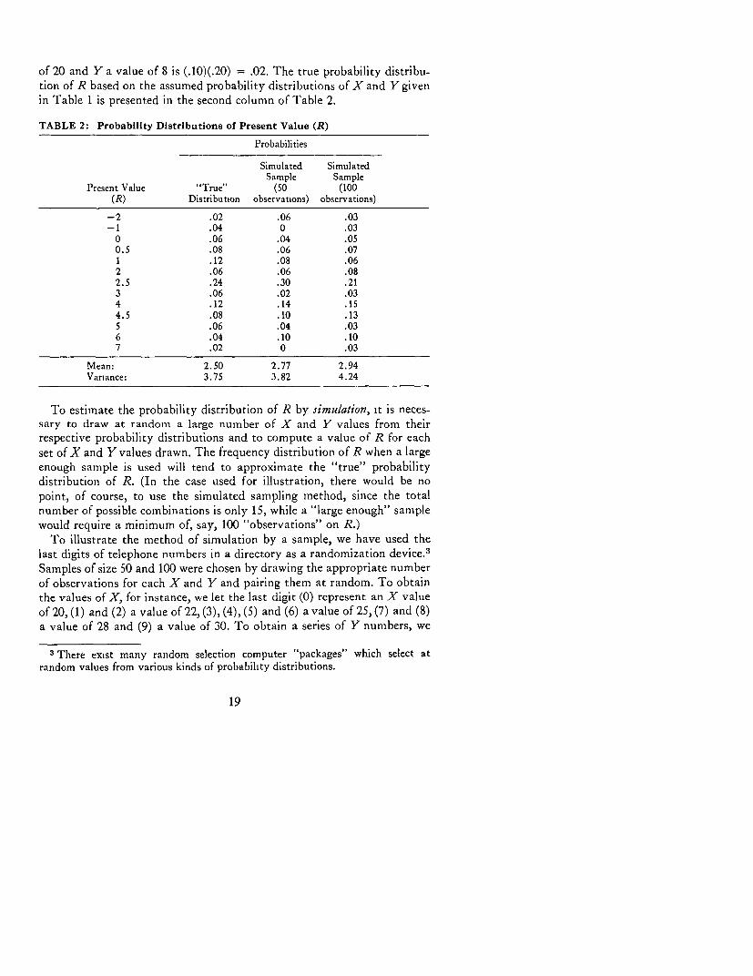
of 20 and Y a value of 8 is (.10)(.20) = .02. The true probability distribu-tion of R based on the assumed probability distributions of X and Y given

in Table 1 is presented in the second column of Table 2.

TABLE 2: Probability Distributions of Present Value (R)

Probabilities

Simulated SimulatedSample Sample

Present Value "True" (50 (100(R) Distribution observations) observations)

-2 .02 .06 .03-I .04 0 .03

0 .06 .04 .050.5 .08 .06 .071 .12 .08 .062 .06 .06 .082.5 .24 .30 .213 .06 .02 .034 .12 .14 .154.5 .08 .10 .135 .06 .04 .036 .04 .10 .107 .02 0 .03

Mean: 2.50 2.77 2.94Vanance: 3.75 3.82 4.24

To estimate the probability distribution of R by simulation, it is neces-sary to draw at random a large number of X and Y values from theirrespective probability distributions and to compute a value of R for each

set of X and Y values drawn. The frequency distribution of R when a large

enough sample is used will tend to approximate the "true" probability

distribution of R. (In the case used for illustration, there would be no

point, of course, to use the simulated sampling method, since the totalnumber of possible combinations is only 15, while a "large enough" sample

would require a minimum of, say, 100 "observations" on R.)To illustrate the method of simulation by a sample, we have used the

last digits of telephone numbers in a directory as a randomization device. 3

Samples of size S0 and 100 were chosen by drawing the appropriate number

of observations for each X and Y and pairing them at random. To obtainthe values of X, for instance, we let the last digit (0) represent an X value

of 20, (1) and (2) a value of 22, (3), (4), (5) and (6) a value of 25, (7) and (8)a value of 28 and (9) a value of 30. To obtain a series of Y numbers, we

3 There exist many random selection computer "packages" which select atrandom values from various kinds of probability distributions.

19

let a last digit of (0) and (1) represent a Y value of 8, (2), (3), (4), (5), (6)and (7) a value of 10 and (8) and (9) a value of 12. The probability distribu-tions of R corresponding with 50 and 100 pairs of randomly selected Xand Y values from their respective probability distributions are presentedin Columns 3 and 4 of Table 2.

The third procedure consists of calculating the mean and the variance ofthe present value (R) and interpreting the results in terms of a normaldistribution. This is, of course, only an approximation procedure, sincewe know already that in our case, the "true" distribution is a discretedistribution (i.e. the variables in which we are interested take on onlydiscrete values) and the probabilities do not follow an exact pattern aswould be expected from a normal distribution. To begin with, however, letus see how to calculate the mean and the variance of R and how to interpretthese in terms of a normal distribution.

Denote the means of X and Y by X and Y respectively, and their vari-ances by V(X) and V(Y). In our case, (from the basic data presented inTable 1):

X = E (probability of an event i)(X,)

= (.10) (20) + (.20) (22) + (.40) (25) + (.20) (28) + (.10) (30) = 25Y = E (prob i) (Y,)

= (.20) (8) + (.60) (10) + (.20) (12) = 10V(X) = E (prob i) (X -X)2

= (.10) (-5)2 + (.20) (-3)2 + .20 (3)2 + .10 (5)2 = 8.6

and

V(Y) = E (prob i) (Y, - Y)2= .20 (-2)2 + .20 (2)2 = 1.6

Given these data, it is a simple matter to calculate the mean, R, and thevariance, V(R), of the present value as follows (it will be recalled that therevenue is discounted to present value by a factor of .5):

R = (.5) (X) - Y= (.5) (25) - 10 = 2.5

andV(R) = (.5)2 V(X) + V(Y)

= (.25) (8.6) + (1.6) = 3.75

assuming that X and Y are not correlated.4

4 See Annex for the mathematical derivation of the formulae. Note that themean and variance calculated by these formulae are the "true" mean and varianceof R.

20

To determine the probability that R is less than any value, Ri, one com-

putes the ratio (R ) and looks up the probability in a table of the

standard normal distribution. The cumulative distribution based on theassumption that R approximates a normal distribution is given in the lastcolumn of Table 3, and is presented graphically in Figure 1. For comparison,the cumulative probabilities from the "true" probability distribution andthe simulated samples are also presented in Table 3 and Figure 1. A cumula-tive distribution shows the probabilities that the event will be less than astated value.

TABLE 3: Cumulative Probability Distribution of RCumulative Probabilties, Prob. (R < R,)

Present ApproximationValue "True" Sample 50 Sample 100 by Normal

R, Distribution Observations Observations Distribution

-2.0 0.02 0.06 0.03 0.01-1.0 0.06 0.06 0.06 0.04

0 0.12 0.10 0.11 0.100.5 0.20 0.16 0.18 0.151.0 0.32 0.24 0.24 0.222.0 0.38 0.30 0.32 0.402.5 0.62 0.60 0.53 0.503.0 0.68 0.62 0.56 0.604.0 0.80 0.76 0.71 0.784.5 0.88 0.80 0.84 0.855.0 0.94 0.90 0.87 0.906.0 0.98 1.00 0.97 0.967.0 1.00 1.00 1.00 0.99

Discussion of Alternative Estimating Procedures

The brief illustration and comparison of results of the two estimationprocedures-the simulation method and the mathematical method-suffices to point up, at least in principle, the possible advantageous featuresand the shortcomings of both methods.

For simulation the project appraiser needs no knowledge of the prob-ability calculus whatsoever. There is no chance of making any error in thecalculations. All the appraiser needs to do is to present the computer witha model and the constant values or probability distributions of the relevantparameters and variables, and the computer (with a programmer's aid) cangrind out an estimated probability distribution of the desired aggregatemeasure. Furthermore, this method requires no assumptions with respectto the relevant final distributions, since the calculated sample gives directlyan estimate of the "true" distribution, whatever its shape.

21

FIGURE ICUMULATIVE PROBABILITY DISTRIBUTIONS OF PRESENT VALUE

Probab/lty

1.0

.9

'true"

7/7 -norma/

6somple simulation

5S ( t: {/00 observatlons)

4

.1 - I.

-3 -2 -/ 0 / 2 3 4 5 6 7

Present volue

The primary disadvantage of the simulation method is its completereliance on the availability of a computer. Furthermore, any "run" ishighly specific to the postulated inputs. If any variations in the assump-tions or in the project itself are to be investigated, a new computer "run"is necessary. Frequently, while still in the field, an appraisal team may wishto pursue consideration of alternatives based on the results of a previousanalysis. With simulation this may not be feasible. Another unresolvedissue is the optimum sample size. However, since in most cases very littlecomputing time on a large computer will be required, the practical solutionmight be to choose a relatively large sample, or to devise a sampling pro-cedure by stages with a statistical test to determine whether additionalobservations should be calculated. In this case, the variance would be esti-mated from an initial sample. This in conjunction with preassigned con-fidence intervals can be used to determine the adequate sample size.

22

The mathematical method is only useful if one wishes to consider arelatively simple model consisting of aggregation of only a few major un-certain variables. In this case, the method is cheap, requiring little morethan pencil and paper and a desk calculator. Furthermore, once the meanand the variance have been calculated for one set of parameters, it is easyto estimate the effects of changes in any of the parameters or probabilitydistributions of the important variables on the mean and variance of thedesired aggregate measure.

The mathematical method does require some minimal knowledge of theprobability calculus; however, this is no major problem. An investmentappraiser usually knows how to calculate means and variances and can beeasily familiarized with a few basic rules needed for deriving the mean andvariance of an aggregative measure.5 The real problem is to determine howuseful it is to know the mean and the variance if one does not know theexact shape of the probability distribution of the aggregate measure.

There are several ways of "sweeping the distribution problem under thetable." None, however, are completely satisfactory. There are, for instance,some decision-makers, or so it is assumed in much of the literature on riskappraisal, whose objective function is such that they require to know onlythe mean and variance. This aspect of the problem is further discussed inthe following chapter. At least very superficially, however, it may be seri-ously questioned whether decision-making under uncertainty can be gen-erally reduced to a maximization of a weighted function of a mean andvariance of some measure of income. On the other hand, particularly whenone wishes to consider various alternative ways of designing a given projectwhich will be subject therefore, to essentially the same kind of probabilitydistribution, it may be quite sufficient to have information on the meansand variances of alternative designs.

Then there are, of course, quite a number of projects for which the ag-gregate measure of the net benefits would be approximately characterizedby a normal distribution, which is completely specified once the mean andvariance are known. Say, for instance, that the present value is simply thesum of a string of discounted annual net benefits, each of which are assumedto follow a normal distribution. In this case, the present value would in-deed be a normal distribution as well. 6 Furthermore, even if the annual netbenefits were not normally distributed, the present value distributionwould still be approximately normal, if a large number of annual benefitswith approximately equal weights were to be summed (i.e. if the interest

5 Some of these basic rules are given in the Annex.6 The internal rate of return, however, would not be exactly normally distributed.

23

rate were relatively low).7 There is no assurance, however, that the inter-

pretation of the calculated mean and variance of a present value of an

internal rate of return in terms of a normal probability distribution is a

reasonable procedure in all cases. It is first of all an empirical question

how much the true distribution deviates from normality; also it depends

how sensitive the decision criteria are.The data presented in Table 3 illustrates the problem fairly well. The

true distribution of the aggregate measure R is certainly not a normal

distribution, yet the cumulative probabilities estimated by using the mathe-

matical expectations method and interpreting the mean and variance in

terms of a normal distribution do not differ much from the "true" cumula-tive probabilities. Certainly, the distribution derived from a sample of 100

does not give better estimates (though a sufficiently large sample would

have had at least a high probability of doing better).In summary, as a matter of general practice the simulation method is the

preferable method whenever a complete probability appraisal is desired.

With computers becoming increasingly accessible and appropriate programsmore generally available, the simulation method is likely to be actually less

costly both in terms of manpower and mathematical skills required than

the mathematical method. In addition and quite importantly, simulationis likely to give a better estimate of the true distribution than can be ex-

pected from assuming a normal distribution. The mathematical method is

likely to prove useful, however, if partial analysis of the impact of uncer-

tainty in a few selected variables is desired and quick approximate answers

are needed.For the remainder of this chapter only the mathematical appraisal

method is used in order (a) to show how, in general, the results from a prob-

ability appraisal may differ from the results obtained by a conventionally

practiced project appraisal, and (b) in order to illustrate further some

essential rules from the probability calculus. The simulation procedure is

not very well suited for deriving generalizations and is simple and straight-

forward enough not to require further illustrations.8

Conceptual Problems Related to Probability Ippraisal

Throughout the discussion so far we have assumed that the reason for

making a probability appraisal is that decision-makers are interested in

knowing not merely a single-valued measure of a project's outcome, such

7 This is shown by the Central Limit Theorem.8 See, however, Chapter VI.

24

as the one most likely or an average, but also other possible outcomes andtheir respective probabilities. Under the heading of "Biased estimates"below we explain why probability appraisal is desirable even if the decision-maker were to be satisfied with merely knowing a single valued estimate.Another problem discussed in this section is the problem of estimating theprobability distribution of the present value or the internal rate of returnfor stochastic variables, some of which are correlated.

Biased estimates

Even if the decision-maker were interested only in a single point estimateand not in the entire probability distribution, it would be desirable to do aprobability appraisal in some cases in order to avoid consistent errors ofestimation.

One example is the practice of aggregating most likely values (modes) ofvarious variables. To illustrate the folly of this method of aggregation,consider first a simple case where one is interested in estimating the mostlikely revenue from forecasts of price and sales. Say the market analystpredicts a 60 percent chance that the price will be $10 and a 40 percentchance that the price will be only $5. Sales are given a 60 percent chanceto be 100 units and a 40 percent chance to be 50 units. The most likelyrevenue calculated from the most likely price and most likely sales isobviously $1,000. However, a probability appraisal would have clearlyshown that this is not the correct estimate of the most likely revenue.Assuming that price and sales are not correlated, the true probabilitydistribution of revenue is as follows:

Price Sales Probability Revenue10 10 .36 1,00010 5 .24 5005 10 .24 5005 5 .16 250

Clearly, the most likely revenue is $500 (with a probability of .48) and not$1,000 (with a probability of .36). In general, when an aggregate measureis the (weighted) sum of many different variables or products of variables,the simple aggregation of modes will not give an accurate estimate of thetrue mode of the aggregate measure.

The same reasoning, of course, applies when one is interested in gettinga "conservative" estimate, where such an estimate is defined as an outcomewhich has a large chance of being exceeded. If one were to aggregate such

25

conservative estimates for different prices and sales, etc., the result would

generally be a rate of return with an undefined extent of "conservative-

ness." In fact, to follow such a rule-of-thumb would certainly lead to non-

comparable rates of returns estimates for different projects in terms of the

degree of "conservatism" implied.The problem of bias exists also if one is aggregating means of probability

distributions of several elementary events to estimate a mean of the ag-

gregate. Fortunately, there are likely to be many cases when such estimates

are not biased, however. One such case is if the aggregate is a function

linear in the uncertain variables. Say present value (R) is a sum of the

discounted benefits (B) in several years. Then the mean of revenue (R) is

the sum of the discounted mean annual benefits (B), i.e.

R = Bo + A,1 + a2B2 . ................ (8)

where a = (1 + r)'1 and r is the discount rate.

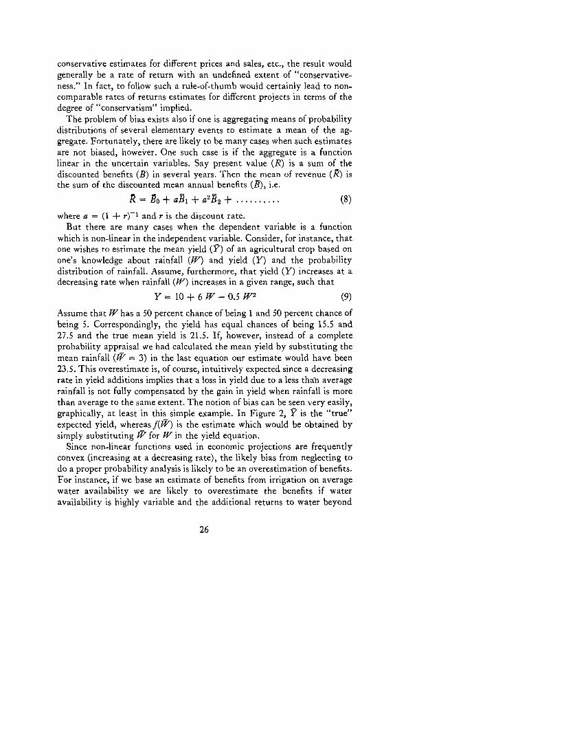
But there are many cases when the dependent variable is a function

which is non-linear in the independent variable. Consider, for instance, that

one wishes to estimate the mean yield (Y) of an agricultural crop based on

one's knowledge about rainfall (W) and yield (Y) and the probability

distribution of rainfall. Assume, furthermore, that yield (Y) increases at a

decreasing rate when rainfall (W) increases in a given range, such that

Y = 10 + 6 W - 0.5 W2 (9)

Assume that W has a 50 percent chance of being 1 and 50 percent chance of

being 5. Correspondingly, the yield has equal chances of being 15.5 and

27.5 and the true mean yield is 21.5. If, however, instead of a complete

probability appraisal we had calculated the mean yield by substituting the

mean rainfall (WY = 3) in the last equation our estimate would have been

23.5. This overestimate is, of course, intuitively expected since a decreasing

rate in yield additions implies that a loss in yield due to a less tha-n average

rainfall is not fully compensated by the gain in yield when rainfall is more

than average to the same extent. The notion of bias can be seen very easily,

graphically, at least in this simple example. In Figure 2, Y is the "true"

expected yield, whereas f(W) is the estimate which would be obtained by

simply substituting W7V for W in the yield equation.

Since non-linear functions used in economic projections are frequently

convex (increasing at a decreasing rate), the likely bias from neglecting to

do a proper probability analysis is likely to be an overestimation of benefits.

For instance, if we base an estimate of benefits from irrigation on average

water availability we are likely to overestimate the benefits if water

availability is highly variable and the additional returns to water beyond

26

FIGURE 2ILLUSTRATION OF BIAS WHEN YIELD IS CALCULATED AS A

FUNCTION OF AVERAGE RAINFALL

Yield

30 _

- Y2

205-

Y= f(W2 ,. I

------------------ 7

20

/0 f

0 / 2 3 4 5W/ WI W2

Rainfall

the average amount are small in comparison with the loss in revenue due toan amount of water less than the average. A likely source of a similar biasin project appraisal is the calculation of cost-benefits on the basis of anaverage life of the investment. The present value as a function of invest-ment life certainly increases at a decreasing rate. Thus there is a possibilityof bias similar to that shown in Figure 2, if for instance there is held to bean equal possibility of the life being 10 years or 50 years. The bias can bequite large, particularly if the discount rate is high and the average invest-ment life fairly short. Several possible sources of such biases are discussedbelow. The point to be made is that it may be desirable to do a complete

27

probability appraisal even if the appraiser is only interested in a single-valued estimate and not in the entire probability distribution of somemeasure of a project's benefits.

Correlation

A major problem in appraising a project subject to stochastic events iscorrelation. Generally, the existence of correlation indicates incompletemodel specification. Therefore, if significant correlations are suspected, thebest way to avoid misleading predictions is explicitly to recognize furtherunderlying systematic relationships among variables and to substituteuncorrelated variables. The problem of correlation and how to cope with itcan be best illustrated by a few examples.

Consider that the objective is to estimate revenue (R) based on priorestimates of price (T) and sales (S), i.e.

R = (T)(S) (10)

Assume, furthermore, that the price is believed to have a 50-50 chance ofbeing 1 or 3 and similarly sales have a 50-50 chance of being 200 or 400.The distribution, mean and variance of the revenue, assuming no correla-tion, are as follows:

.i . Combination Revenue Mean andProbability (Price, Sales) (R) Variance

.25 (1,200) 200 R= 600

.25 (1,400) 400 V(R) = 140,000

.25 (3,200) 600

.25 (3,400) 1,200

By contrast, if price and sales in the above example had been perfectlycorrelated, if for instance, whenever sales are 200, price is 3, and wheneversales are 600, price is 1, then the "true" distribution of revenue, the meanand variance would have been as follows:

Probabili Combination Revenue Mean andty (Price, Sales) (R) Variance

.50 1,400 400 R= 500

.50 3,200 600 V(R) = 10,000

Clearly, whether or not price and sales are correlated makes quite a

28

difference in how we should calculate the distribution of revenue. Bothmean and variance of the product of price and sales are different, dependingon the extent of correlation. The correlation between price and sales couldhave been accounted for by specifying an additional equation describingthe relationship between sales and price as follows:

T= 5-.01 S (11)

or if price and sales are not perfectly correlated as implied by the lineardemand function (11), then by

T = 5-.01 S + e (12)

where e represents random effects on price not correlated with sales. Themathematical equations for deriving the mean and variance of the revenuein both the correlated and uncorrelated case are presented in the Annex.

Another likely source of correlation is that two or more variables arerelated in a systematic way to a third variable. For illustration, considerthat we wish to calculate the probability distribution of a total revenue onthe basis of what we believe are the probability distributions of revenuefrom two sources, R1 and R2, i.e.

R = R1 + R2 (13)

given the following data:

Probability Revenue (1 ) .b Revenue (2)Revenue ( Probability

.50 50 .50 40

.50 90 .50 60

and disregarding the possibility of correlation, the probability distributionof total revenue, its mean and variance are summarized below:

Probability Combination Total Mean and[RI, R2] Revenue (R) Variance

.25 50, 40 90 R= 120

.25 50, 60 110 V(R) = S00

.25 90, 40 130

.25 90, 60 150

If, however, the uncertainty in both revenues had the same underlyingcause (say both would be the higher of the given values if a protective

29

tariff were to prevail and enactment of the legislation were given a 50-50

chance), then R1 and R2 are perfectly correlated. The correspondingprobability distribution mean and variance of total revenue would in this

case be as follows:

Prba t . Combination Revenue Mean andP[R, R2] (R) Variance

.50 (50, 40) 90 R= 120

.50 (90, 60) 150 V(R) = 900

Note that correlation does not affect the mean of a sum. However, thevariance can be substantially altered by the presence of correlation. Further

specification of the model would have given an explicit equation for the

close relationship of the respective revenues with the size of tariff (Z). Fromour data we can interpolate that these relationships may be as follows:

R1 = 50 + 4 Z (14)

and

R 2 =40+2Z (15)

Adding these equations to the model we would substitute (14) and (15)

into (13), i.e.

R = 90 + 6 Z (16)

and estimate the probability distribution of total revenue, its mean and

variance directly from this equation, as follows:

Proabt . Tariff Total Mean and(Z) Revenue Variance

.50 0 90 R= 120.50 1.0 150 V(R) = 900

It should be recalled, as noted earlier, that the method of calculating allpossible outcomes is not an operational procedure and is used here only to

illustrate concepts. In the next section we will show how to estimate the

mean and variance of total revenue by using the mathematics of expecta-tions.9

9 The mean and variance can be readily calculated from equation (16). Note thatZ = 5 and V(Z) = 25. Then R = 90 + 6 (5) = 120 and V(R) = (62)(25) = 900.

30

The problem of correlation, then, is the problem of accounting for rela-tionships between the included variables themselves, and between includedvariables and excluded variables. Since in any practical appraisal only afew relationships can be explicitly stated, one could not possibly hope forthe removal of all correlation. The best one can hope for is that the problemis recognized and understood, and that the appraiser explicitly accountsfor the more important relationships and makes judgments about theirquantitative nature.

Specific Uncertainty Problems in Project Appraisal

The purpose of the ensuing discussion is twofold: to illustrate how tocalculate the mean and variance of the present value and other selectedvariables and to derive some generalizations for assessing projects subjectto uncertainty. The operational uses of the mathematical estimation pro-cedure are, of course, limited to highly stylized appraisal models. These,however, are often quite useful at least as preliminary exercises prior to amore complete appraisal.

Uncertainty about annual net benefits

Let us begin by assuming that the appraisal has proceeded to the pointof having an estimate of a stream of annual benefits (positive or negative),that the annual benefits can be estimated in terms of probability distribu-tions and that the discount rate is known. The expected (mean) presentvalue (R) is then simply a weighted sum of the expected (mean) annualbenefits, i.e.

R = Bo + aBi + a2B2 +.**. (17)

where a = (1 + r)'1 and r is the discount rate. Note that for estimating themean present value it matters not whether successive benefits are corre-lated. The variance of R, V(R), depends very much on the extent of corre-lation between successive benefits. If successive benefits are not correlatedthe variance of the present value is

V(R) = V(Bo) + a2V(B1) + a4V(B 2 ) + .... + a2 l V(Bt) .... (18)

But, if the benefits are perfectly correlated,

V(R) = [\VV(Bo) + a\V(B 1) + a2\V(B 2)

+ .... + a V(B) + .... 2 (19)

31

Equal annual correlated and uncorrelated benefits

The above equations for deriving the mean and variance of the presentvalue can be easily solved when a large number of successive benefits havemeans and variances which are equal or follow a general trend. Let us firstassume that annual benefits consist of a known or unknown level of bene-fits, B, and positive or negative, but from year to year uncorrelated devia-tions from this level, et, such that,

B 1 = B+et (20)

Then, if B is known and et is assumed to be zero on the average, A1 = B andV(B,) = V(e). Since we have assumed that the et in successive years are notcorrelated, the annual benefits are clearly not correlated as well. If B, thelevel of the annual benefits, is not known except in terms of an average B

and a variance V(B), but et is zero in all years, A1 = B and V(B,) = V(B).In this case the annual benefits are perfectly correlated. We now proceedto analyze the corresponding calculations of the mean and variance of thepresent value of a stream of benefits in these two extreme cases.

Regardless of whether successive benefits are correlated, the mean of thepresent value is

R = (, at) B (21)

where a is (1 + r)-1 and r is the discount rate. However, the variance, ofthe present value depends on correlation.' 0 If the successive benefits areuncorrelated, i.e. if the uncertainty is due to year to year fluctuations,

V(R) = (, a2') V(eg) (22)

If the level of benefits is the only source of uncertainty,

V(R) = (7 a,)I V(B) (23)

Derivation of these equations is discussed in the Annex. Values of (5 a2 ')for up to 30 years and 6 percent and 10 percent discount rates are presentedin Annex Table 1.

As should be expected, the variance in the present value is relativelymuch smaller when successive benefits are uncorrelated than when theyare positively correlated. For instance, we may be uncertain whether theannual benefits are plus or minus 30 percent of the mean. No correlationmeans that overestimates are likely to be compensated by underestimates.Perfect positive correlation of all successive benefits means, however, that

10 In all the equations presented here it is assumed that V(et) is the same in allyears, i.e. V(el) = V(e2) = .... = V(e.), where et is the random effect.

32

the same forces are at work, and if we have overestimated the benefits inthe first year overestimation will occur in all subsequent years.

To compare variances it is frequently convenient to use the ratio C =-\/7'i(B1, the so-called coefficient of variation. C is then a measure of therelative variance and allows us to make some general statements about theimpact of various kinds of uncertainty on the uncertainty implied for theoverall returns for a project.

The coefficient of variation of the present value, CR, when successivebenefits are perfectly correlated simply equals the coefficient of variationof the annual benefits, CB, i.e.

R~ Ea /7X B (24)

or

CR = CB

However, if successive benefits are no t correlated, the coefficient of variationof the present value is

CR = ( / / a') CB (25)

Table 4 gives the ratio of the coefficients of variation of the present valueto the coefficient of variation of the annual benefits for selected life spansof projects and discount rates. As is to be expected, the longer the life ofthe project and the lower the discount rate, the more "errors" of estimationin the true benefits compensate for each other. Quite generally, Table 4shows that year to year variations in benefits, perhaps due to weather orother non-systematic errors (in terms of persistence over time), are rela-tively quite unimportant in assessing the uncertainty about the presentvalue (or rate of return). In general, the standard deviation of the presentvalue derived from a given standard deviation of year to year correlatedannual benefits will be approximately 3 to 4 times as large as when derivedfrom the same standard deviation of year to year uncorrelated benefits.

TABLE 4: Ratio of Coefficient of Variation of Present Value (CR) to Coefficientof Variation of Successively Uncorrelated Annual Benefits (CB)

(for a stream of equal mean annual benefits)

Discount RateNumberof Years 6% 10% 20%

CR/CR equals:10 .32 .33 .3420 .24 .25 .3130 .20 .23

33

A coefficient of variation as large as 0.5, for instance, in the annual bene-fits deriving from year to year uncorrelated "errors" about an assumed

estimated mean level of benefits, would result in a coefficient of variationof approximately only 0.15 in present value. In other words a 95 percent

confidence statement (approximately plus and minus 2 standard deviations,assuming a normal distribution), such that the annual benefits might be

fluctuating within a range of 0 to 200, would reduce to a similarly definedconfidence statement that the present value of the stream of benefits will

be within the range of 700 to 1,300. Whereas, if successive annual benefitswere perfectly correlated, the corresponding confidence statement withrespect to the present value of the stream of benefits would have given arange of 0 to 2,000.

For another illustration of the effect of correlation consider the data in

Table 5. The benefits in this case are accruing over an eight-year period.The discount rate is assumed to be 8 percent. If successive values of the

benefits are not correlated the variance of the present value is 1,187 and

the standard deviation 34. Uncorrelated benefits would be an appropriateassumption, if the source of the variability of outcome is a result of year to

year changes in climate or prices which in turn are not correlated. If, how-ever, the uncertainty is for instance the direct consequence of not knowingconsumer reaction to a new product, the benefit can be assumed to be al-

most perfectly correlated. That is, in each of the 8 years benefits may be

high or low, but if consumers respond unfavorably the benefits will be low

in every year, and if the new product is favorably received the benefits will

be high in every year. Assuming perfect correlation, the same assumptionsabout the variances of the benefits in each year will result in a variance of

the present value of 9,149 or a standard deviation of 96.That uncorrelated fluctuations in annual benefits are relatively unim-

TABLE 5: Hypothetical Data for Calculating a Variance of the Present Valuewhen Benefits from Successive -Years are Uncorrelated or PerfectlyCorrelated

I ata

2 t V(B,) I/V(Bt) V(R)

I .93 .86 225 15 Uncorrelated

2 .86 .74 400 20 V(R) = 1,1873 .79 .63 225 15 Standard Deviation4 .74 .54 200 14 (\T(R_N)) = 345 .68 .46 256 16 Correlated6 .63 .40 289 17 V(R) = 9,1497 .58 .34 324 18 Standard Deviation8 .54 .29 361 19 (A/V(R)) = 96

34

TABLE 6: Elasticity of Variance of Present Value of a Stream of Benefits withRespect to Variance of Successively Uncorrelated Benefits (whenBt = B + et)

Duration of Discount RateBenefits(years) 6% 10% 20%

(1) V(eC)= V(B)10 .093 .097 .09820 .053 .060 .08830 .040 .051 -

(2) V(e) = 2 V(B)10 .171 .177 .18020 .100 .114 .16330 .076 .097 -

(3) V(et) = 3 V(B)10 .236 .244 .24520 .143 .162 .22530 .111 .138 -

portant for the uncertainty about the present value (or rate of return onthe project) can be shown by considering the simultaneous contribution ofthe variances from successively correlated and uncorrelated benefits on thevariance of the present value of a stream of benefits. If the variance is anadditive function of the variance in the level of benefits and the variancedue to year to year fluctuations such that

V(B,) = V(B) + V(e,) (26)

Correspondingly, the variance of the present value of such a stream ofbenefits is

V(R) = (fi a,)2 V(B) + (i a2') V(et) (27)

To measure the relative sensitivity of the variance of present value tovariances from different sources it is now useful to calculate elasticities, i.e.the percentage change in the variance of the present value to a one percentchange in the variance of a contributing factor." When the factors are

ii The elasticity (E) of V(R) with respect to V(ei) is as follows:

EV(et) = I

E_ a2 ' V(et)

These elasticities for various interest rates and relative sizes of V(et) are presentedin Table 6. The elasticity of V(R) with respect to V(B) is: 1 - Ev(ei).

35

additive and not correlated, these elasticities add up to unity. Table 6 giveselasticities of the coefficient of variation of the present value with respectto the coefficient of variation of the successively uncorrelated benefits.Clearly, unless the project life is very short and the year to year fluctua-tions are very large relative to the uncertainty about the level of benefits,the variance of the present value is quite insensitive to the projected yearto year uncorrelated variations in benefits.

For an illustration, consider an irrigation project whose life is 20 yearswhile the discount rate is 10 percent. The average expected annual returnis not known with any certainty, but is estimated to be a normal distribu-tion with a mean of 100 and a standard deviation of 10. Furthermore, nomatter what average level of returns will actually occur, there are expectedyear to year fluctuations. If the standard deviation of these fluctuations isalso 10, the total variance of the present value turns out to be about 30,800(the mean of the distribution of present value is 850 and the standarddeviation is 175). Neglecting the year to year uncorrelated errors thevariance would have been 28,960 and the standard deviation 170. Hence,the uncorrelated year to year variations "contribute" only 6 percent tothe variance of the present value. The elasticity with respect to thesefluctuations in Table 6 is .06.

A!nnual benefits contain an uncertain trend

One case of strong serial correlation in connection with variances ofannual benefits is, of course, the presence of trend, i.e. the uncertaintyabout benefits derived in a particular year arises primarily from not know-ing the trend. Benefits may increase over time because a structure must beconstructed to an excessive capacity which will be only increasingly usedwith time, or in general, because of an increase in demand over time forthe services generated by the investment. Benefits may also decline becauseof progressive physical or technological obsolescence of the investment. Forillustration, let us imagine that an annual benefit (Bt) can be representedby the following equation:

Bt = Bo + bt + et (28)

where Bo is the benefit in the initial year, b is the annual growth and, t isthe number of years since the initial benefits have occurred and et rep-resents many random effects which can make an annual benefit deviatefrom its normal trend.

Given the growth-of-benefits equation (28) the formula for calculatingthe mean and variance of present value (R and V(R)), based on knowledge

36

of Bo and V(Bo), b and V(b) and V(e) (e is assumed to be zero) are asfollows:

R = (, a,) Bo + (7ta') b (29)

and

V(R) = ( a')2 V(Bo) + ( tal)2 V(b) + ( a2 ') V(e) (30)

On the basis of the above equations, it is first interesting to note therelative sensitivity of R to Bo, the initial level of benefits and to b, theannual average growth. Here again we use the elasticity concept, i.e. thepercentage change in the mean present value in response to the percentagechange in the mean growth, etc. Obviously, this sensitivity depends on therelative size of the annual growth, the discount rate and the life of theproject. Table 7 gives the elasticity with respect to changes in b, the growthrate for two levels. The high level corresponds with a doubling of the initial

TABLE 7: Elasticity of the Mean Present Value (R) with Respect to MeanGrowth (6) and Mean Initial Benefits (fl)'

Elasticity Discount RateProject with

Life Respect to: 6% 10% 20%

High Average Annual Growth (Z B= )

10 years o .33 .32 .29fo .67 .68 .71

20 years Z .46 .43 .35Ao .54 .57 .65

30 years Z .53 .48 .37go .47 .52 .63

Low Auerage Annual Growth = B.

10 years 3 .20 .19 .17So .80 .81 .83

20 years Z .30 .27 .21fBo .70 .73 .79

30 years Z .36 .32 .23,Ao .64 .68 .77

The elasticity of R with respect to = ( ) A

(E tat) Z

benefits in ten years (i.e. b = Bo/10) and the low rate implies a doublingof the initial benefits by the twentieth year (i.e. b = So/20). For instance,given a project life of 10 years, a low growth rate and a 20 percent discount

37

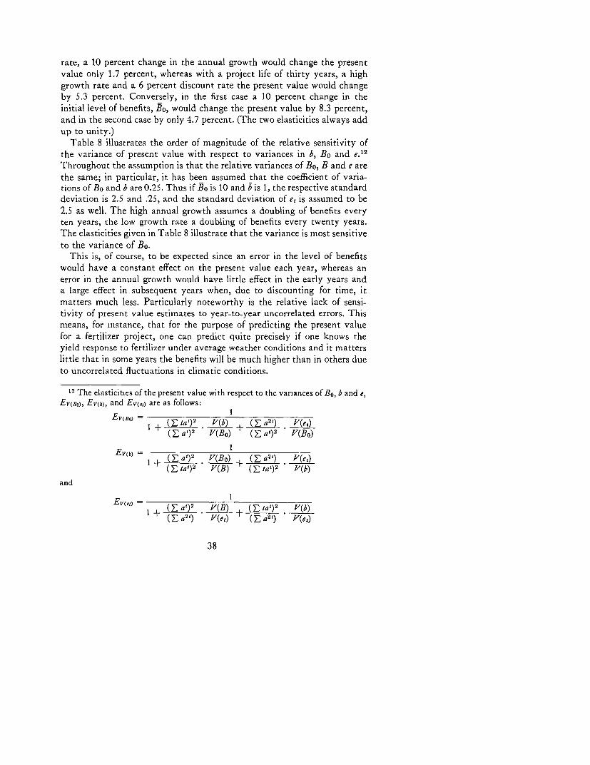
rate, a 10 percent change in the annual growth would change the present

value only 1.7 percent, whereas with a project life of thirty years, a high

growth rate and a 6 percent discount rate the present value would change

by 5.3 percent. Conversely, in the first case a 10 percent change in the

initial level of benefits, Bo, would change the present value by 8.3 percent,

and in the second case by only 4.7 percent. (The two elasticities always add

up to unity.)Table 8 illustrates the order of magnitude of the relative sensitivity of

the variance of present value with respect to variances in b, Bo and e.12

Throughout the assumption is that the relative variances of Bo, B and e are

the same; in particular, it has been assumed that the coefficient of varia-tions of Bo and b are 0.25. Thus if Bo is 10 and b is 1, the respective standard

deviation is 2.5 and .25, and the standard deviation of et is assumed to be

2.5 as well. The high annual growth assumes a doubling of benefits every

ten years, the low growth rate a doubling of benefits every twenty years.

The elasticities given in Table 8 illustrate that the variance is most sensitive

to the variance of Bo.This is, of course, to be expected since an error in the level of benefits

would have a constant effect on the present value each year, whereas an

error in the annual growth would have little effect in the early years and

a large effect in subsequent years when, due to discounting for time, it

matters much less. Particularly noteworthy is the relative lack of sensi-

tivity of present value estimates to year-to-year uncorrelated errors. This

means, for instance, that for the purpose of predicting the present value

for a fertilizer project, one can predict quite precisely if one knows the

yield response to fertilizer under average weather conditions and it matters

little that in some years the benefits will be much higher than in others due

to uncorrelated fluctuations in climatic conditions.

12 The elasticities of the present value with respect to the variances of Bo, b and e,Ev(BO), EV(b), and Ev(ei) are as follows:

EB + ( ta')2 V(b) + ( all) V(et)(ZE a9)2 V(Bo) (V a9) J(Bo)

Ev(b) = 1)1b + (J a92 V(Bo) (E all) V(et)

( tat)

2 V(B) +(E tat )2 V(b)

and

+ (Ea92 . V(B) + (Eta92 . V(b)(E a2l) V(e) (Ea2l) V(e3

38

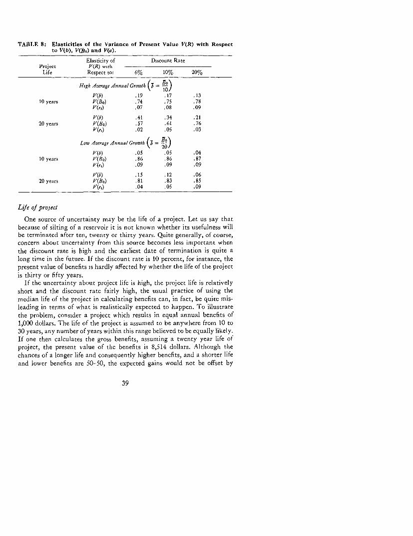
TABLE 8: Elasticities of the Variance of Present Value V(R) with Respectto V(b), V(Ro) and V(e).

Elasticity of Discount RateProject V(R) with --

Life Respect to: 6% 10% 20%

High Zverage Annual Growth =o

V(b) .19 .17 .1310 years V(Bo) .74 .75 .78

V(et) .07 .08 .09

V(b) .41 .34 .2120 years V(Bo) .57 .61 .76

V(e,) .02 .05 .03

Low Average Annual Growth (=.

V(b) .05 .05 .0410 years V(Bo) .86 .86 .87

V(e,) .09 .09 .09

V(b) .15 .12 .0620 years V(Bo) .81 .83 .85

V(eg) .04 .05 .09

Life of project

One source of uncertainty may be the life of a project. Let us say thatbecause of silting of a reservoir it is not known whether its usefulness willbe terminated after ten, twenty or thirty years. Quite generally, of course,concern about uncertainty from this source becomes less important whenthe discount rate is high and the earliest date of termination is quite along time in the future. If the discount rate is 10 percent, for instance, thepresent value of benefits is hardly affected by whether the life of the projectis thirty or fifty years.

If the uncertainty about project life is high, the project life is relativelyshort and the discount rate fairly high, the usual practice of using themedian life of the project in calculating benefits can, in fact, be quite mis-leading in terms of what is realistically expected to happen. To illustratethe problem, consider a project which results in equal annual benefits of1,000 dollars. The life of the project is assumed to be anywhere from 10 to30 years, any number of years within this range believed to be equally likely.If one then calculates the gross benefits, assuming a twenty year life ofproject, the present value of the benefits is 8,514 dollars. Although thechances of a longer life and consequently higher benefits, and a shorter lifeand lower benefits are 50-50, the expected gains would not be offset by

39

the expected losses. In fact, the "true" expected present value, i.e. R, is8,253 dollars. Furthermore, the chance of realizing a present value whichis 1,000 dollars less than the one projected based on the median life of theproject is about 30 percent, whereas the chance of getting 1,000 dollarsmore is zero.

Estimating probability distributions of annual benefits

Attention in this section focuses on selected general problems in esti-mating the probability distribution of the benefits in each year by aggre-gating probability distributions of various factors. Besides being the build-ing blocks for estimating present value of the project, the probabilitydistributions of the annual benefits may be of interest as such. A highreturn in one year may not compensate fully for a low return in anotheryear for many reasons although the average return is satisfactory. It isoften assumed that unstable benefits from year to year are less desirablethan a stream of benefits of equal annual magnitudes, because the cost ofborrowing is higher than the rate of return on savings or because of dimin-ishing marginal utility of income. It is just possible, however, that a nationmay prefer a project which yields unstable returns over the years. Considerfor instance a nation which must decide between two projects which overthe years would produce an equal amount of food per dollar invested. Itwould be quite in the national interest to prefer a project with a highlyfluctuating food output, if this nation could count on getting food grants(or soft loans) in years when its domestic food supply was insufficient tofeed the population, and if in food surplus years the surpluses could beeffectively used for generating investment and economic growth.

Estimation of the annual benefits involves a careful accounting of manyvariables and relationships between variables. It is not possible to give anygeneral rules for deciding how many variables and relationships should beexplicitly considered. A probability appraisal may sometimes suggest con-sideration of more variables and relationships than would be otherwiseexplicitly considered, as it is sometimes easier to assess the probabilitydistribution of a simple than that of a more complex event. However,generally it is sufficient to estimate the probability distributions of thevariables and parameters which one would consider implicitly withoutprobability appraisal.

The major problem in estimating the aggregated probability distributionof the annual benefits is once again correlation. Say the annual operatingcosts are estimated by summing costs of various inputs. The uncertaintyabout each cost item arises from not knowing exactly (a) what quantity ofthe input will be needed and (b) the price of the input. Both the quantities

40

and the prices will often be partially correlated. Only a careful examinationof the data and a thorough understanding of the underlying relationshipscan lead to realistic appraisal of the approximate extent of correlation.

It is not possible to give rules for estimating correlations, just as it isimpossible to give general rules for estimating probability distributions. Thepoint to be made here is simply to suggest that the estimated and reportedcost-benefit measure of a project should adequately reflect what the projectappraisers believe to be their best judgment about the correlation betweenprobability distributions as well as the nature of the probability distribu-tions themselves. Otherwise a careful probability analysis may be self-defeating, or in fact misleading. That is to say, if a probability distributionof a complicated event is to be estimated by aggregating probability dis-tributions, all correlations must be explicitly considered. Otherwise thegains from explicit consideration of many probability distributions maybe offset by the loss from neglecting correlations which would be implicitlytaken into account by a less disaggregated analysis.

Often a large number of costs and benefits are summed to derive thetotal net benefit. If one assumes no correlation when in fact the differentcosts and revenues are perfectly correlated, the true variance may be asmuch as n times the estimated variance when n benefits are summed up,i.e. when two benefits are aggregated the true variance may be two timesthe estimated variance, and when ten revenues and costs are aggregated thetrue variance may be ten times the estimated variance. When many corre-lations are negative, the true variance may be zero or much less than theestimated variance. 13

Summary and Conclusions on Aggregationof Probability Distributions

(a) Judgments about the likelihoods of various outcomes of the ele-mentary events affecting the costs and benefits from a project can

13 Assuming B =Bi + B2 + ... + Bn

and B2 = a2 Bi, .... , Bn = an Bthen the true variance of B is

V(B) = (I + a2 + . .. + a.)' V(BI)whereas, if it were assumed that [B1, B2]. [Bi, B.] are not correlated, thevariance of B would have been calculated as

V(B) = (1 + a' + ...- + a'f) (VBI)

Note that V(B)/V(B) is at maximum when a, = 1, i.e. when the marginal costof capital (or time discount used) is taken to be nil.

41

be combined without great difficulty into an estimate of the approxi-

mate probability distribution of the net present value or the in-

ternal rate of return.

(b) There are available basically two approaches for aggregating prob-

ability distributions into an estimate of the probability distribution

of returns from a project: the simulation by a high-speed computer

of a sample of outcomes based on randomly selected sets of observa-

tions from the probability distributions of inputs, and the mathe-

matical approach of aggregating mathematical expectations into

an estimate of the mean and variance of a project's returns.

(c) For most operational purposes the simulation procedure is the only

feasible method at this time. The simulation procedure requires no

prior assumptions about the nature of the aggregated probability

distribution and no mathematical skills on the part of project ap-

praisers. The major disadvantage of the procedure is the fact that

resulting estimates are specific to one set of input distributions.

(d) A major advantage of the mathematical approach elaborated in

this chapter is that the mean and variance (or standard deviation)

calculations can be made quickly for relatively simple projects when

only a crude estimate of a project's returns based on a few crucial

variables is needed or feasible. The method is useful for deriving

generalizations about the sensitivity of estimates to various ele-

mentary events.

(e) Year to year uncorrelated fluctuations are of relatively minor im-

portance in terms of the probability distribution of overall project

benefits. Instead, one should concentrate on making sure that un-

certainty about the persistent level of costs and benefits is properly

taken into account.

(f) Generally, the problem of estimating the extent of correlation be-

tween the various probability distributions of the elementary events

is likely to prove the most difficult aspect in application of the pro-

cedure. When one estimates directly the probability distribution

of a complicated event (like the rate of return of an investment)

correlations are implicitly taken into account. If such a distribution

is estimated, however, from synthesizing the effects of various con-

tributing factors, correlations must be made explicit and taken into

account. Otherwise, the gains from disaggregation must be seriously

questioned.

42

(g) Probability appraisal is important, not only for estimating the en-tire probability distribution of the return from an investment, butshould be employed also when interest focuses on only the mostlikely return. The usual practice of aggregating averages or mostprobable values of a series of events may in fact not yield a correctestimate of the average or most likely returns of a project asintended.

(h) Just as any quantification of economic relationship is generally onlya question of more or less rather than yes or no, so the optimumextent of quantification of the uncertain elements in project ap-praisal will differ from case to case. In a project appraisal, theimportance of quantifying uncertainty depends not only on theusual limitations of time, effect and cost, but also on the specificdecision context. If the project is one of many unrelated projectsit may be less important to quantify uncertainty than when theproject is very large relative to a country's investment program.

43

IV

PROJECT DECISIONSUNDER UNCERTAINTY

Introduction

After having shown how to incorporate uncertainty into the appraisal ofprojects and portions of projects, we should consider how and to what extentsuch appraisals might be useful for the evaluation of public projects, i.e.for decisions. As indicated earlier, outcomes of decisions which are affectedby the interaction of a great many noncontrollable variables are mostadequately described in terms of probability distribution and sometimesquite adequately by means and variances.' For this reason, and becausethe objective of this paper is to focus primarily on the appraisal of large-scale publicly financed projects, only decision theories which relate tochoices between probability distributions of outcomes (specifically, meansand variances) are discussed here.

Quite apart from the decision problems encountered in the general evalua-tion of projects, there are certain decisions which can only be intelligentlyevaluated if one explicitly studies probability distributions. These are

1 The characterization of probability distributions in terms of means and vari-ances will be seen to be sufficient for some types of distributions, specifically whena normal distribution is approximated, and regardless of normality, if the decision-maker wishes to maximize expected utility and the utility function of income isquadratic.

44

problems of sequential decisions and certain timing aspects of investmentsand the whole subject of the value of gathering additional information.Thesesubjects will also be briefly discussed below.

The first reason for making such appraisals, as indicated in the previouschapter, is of course, quite intuitively, that decision-makers want to knowthe most likely or average outcome as well as the extent of the riskiness ofa project, and a probability distribution or the mean and variance are con-venient indices. The fact that decision-makers ask for this kind of informa-tion is sufficient evidence that decisions are affected by it. If this informa-tion is not supplied by those who are in a position to know best, second-rateinformation may be substituted. On the other hand, if instead of supplyingmeans and variances, the appraiser himself adjusts the estimate of the out-come of a project by some uncertainty factor, the organization is not un-likely to reach investment decisions which are inconsistent and misguidedin terms of higher level policy objectives.

Any theory of economic choice involves the following basic ingredients:(1) the decision agent's preference function, (2) his basic endowment and(3) alternative courses of action with specified consequences. The inter-action between these three aspects of a decision problem can be bestillustrated by a simple hypothetical example.

A Hypothetical Example of the Decision Problem

Consider an individual who is told that he has been selected to receive aprize, and that it is his prerogative to choose between several options. As-sume furthermore, that the same individual has zero wealth and that it istwo days before he will receive his next monthly salary. By option (A) hewill receive 10 dollars at once. Options (B) and (C) will each consist of twopossible outcomes, to be decided by the tossing of a fair coin. By option(B) he would have a 50-50 chance of getting 5 or 15 dollars, respectively.Option (C) would yield him 0 or 20 dollars, each with a 50-50 chance. Theneed for survival would pretty much rule out the latter option. The re-cipient's choice between options (A) and (B) would depend on his subjec-tive preference. If he likes to gamble, or expressed in another way, if hismarginal utility is an increasing function of income, he will choose option(B).

Consider now a second, somewhat different situation in which the sameindividual is told that his options are to receive (A) a prize of 1,000 dollarsat once, (B) 990 dollars at once plus a 50-50 chance of S or 15 dollars and(C) 990 dollars at once plus a 50-50 chance of 0 or 20 dollars, respectively.Clearly, one distinguishing characteristic between the first and the second

45

situation is the fact that by comparison the decision problem appearsto be a trivial one in the latter case. Yet, note that in both instances, thecourse of action and their consequences are identical: 10 dollars for certainvs. 5 and 15, or 0 to 20 with a 50-50 chance respectively. The differencecomes, of course, in the endowment, i.e. the variability of outcomes rela-tive to the total outcomes is small even for the option involving the largestgamble. Hence, it is quite conceivable that the same individual who prefers(A) or (B) to (C) in the first case, will this time prefer option (C) to either(A) or (B).

In a third case, we might conceive of the same individual confrontedwith having to choose between (A) receipt of 1,000 dollars at once, (B) a50-50 chance of receiving 500 dollars or 1,500 dollars, and (C) a 50-50chance at receiving nothing or 2,000 dollars. The endowment and the

variability relative to the average of the respective outcomes in this situa-tion are approximately the same as in the first cited case. However, it isnot at all unlikely that the decision would not be the same as in the firstcase. In fact, we probably would not be too surprised if the same individualwho would have chosen option (B) in the first case would prefer (A) inthis case. This means that an individual's preference function is not a givendatum at all but may vary with the magnitudes of the options.

Finally, we may conceive of a fourth situation in which the same in-dividual is given the option of receiving 1,000 dollars at once, or alterna-tively of participating in a game of chance in which his payoff is to be de-termined by tossing a coin one hundred times. Under option (B) he wouldreceive in each toss either 6 or 16 dollars. Option (C) would pay him 0 to24 dollars. Clearly, these uncertainty options are different from the onesdescribed in the first three cases. The total payoffs are likely to approximateone hundred times the average payoff, i.e. 1,100 and 1,200 dollars foroptions (B) and (C), respectively. Since the total payoff for option (B) canbe expected to approximate a normal probability distribution with astandard deviation of about 50, we would have in fact a 98 percent con-fidence that the payoff from (B) would be greater than 1,000 dollars. Exceptfor an extremely conservative individual, it is therefore quite clear that(B) would be preferred to (A) and most likely (C) would be considered stillmore desirable than (B).2 As a generalization of this case, it may be stated

2 Note that: E(B,) = (.5) (6) + (.5) (16) = 11Var (B,) = .5 (6 - 11)2 + .5 (16 - 11)2 = 25

and E(B) = 100 E(B,) = (100) (11) = 1,100Var (B) = 100 Var (B,) = (110) (25) = 2,500Standard deviation (B) = 50

Similarly, E(C,) = (.5) (0) + (.5) (24) = 12

46

that if plans of action are compared whose outcomes are the sum total ofmany small uncertain outcomes, the decision may be based on a comparisonof the expected outcome from each plan, and the same optimization ruleswhich apply to ordering courses of action with certain outcomes are relevantfor this particular kind of uncertainty problem.

Project Appraisal and Utility Theory

To gain some perspective on the nature of economic decision problemsunder uncertainty it is worthwhile to distinguish first of all between thedecision problem of an individual and of society in a deterministic world,and then to superimpose the problem of uncertain consequences fromalternative courses of action.

Very generally, the objective of economic activity may be regarded asone of maximizing utility or welfare. Utility need not be a measurable ob-ject in order to derive meaningful criteria for an individual's economicdecisions. Instead, it suffices to assume that utility is an increasing functionof income to see that profit maximization is consistent with utility maximi-zation. In a world of certainty, planning for an individual would in factinvolve no decision problem at all. The investment appraiser would examinethe income (or returns) from alternative courses of action and, presumably,the one with the highest returns would be chosen.

Planning for society is more ambiguous, even in a deterministic world.At best, it can be said that given the same minimal assumptions about util-ity (being an increasing function of income for each member of society),society would be potentially better off by maximizing income (ParetoOptimum). That is, if we abstract from possible interdependence of utilityand if the gainers from a particular course of action were actually to com-pensate the losers, social utility would be maximized by maximizing overallincome.3 In reality, compensation does not usually take place. Hence, pub-lic investment decisions usually require a balancing of preferences for acertain income distribution and maximizing overall income.

In dealing with economic choices involving uncertain outcomes, it is

Var (C,) = .5 (0 - 12)2 + .5 (24 - 12)2 = 144and E(C) = (100) (12) = 1,200

Var (C) = 100 (144) = 14,400Standard deviation (C) = 120.

3 Conversely, if utility could be actually measured (not only ordinally in termsof relative preferences) it would be possible to derive a social utility function.However, most economists would agree that the notion of measuring absoluteutility of individuals, quite apart from the impossible task of aggregating, is quiteobsolete.

47

necessary to know something more about an individual's utility function.

Presumably, it is possible to determine an individual's utility function with

respect to uncertain incomes. To be sure, such a utility function measures

relative utility and not absolute utility, that is, the scale on which utility

is measured has no known origin.4 By this theory, the objective of the

individual is to maximize expected utility. If an individual's utility function

is linear, expected utility is maximized whenever he chooses the course of

action which maximizes his expected income. Otherwise, when the utility

function is curvilinear, it is necessary to know the probability distributions

of income from alternative courses of action in order to ascertain which

course maximizes expected utility. If the utility function can be approxi-

mated (in the relevant range) by a quadratic function, expected utility is a

function of the mean and variance of income, i.e. if

U = ao + all + a212 (1)

then

E(U) = ao + a, E(I) + a2 (V(I) + (E(I))2) (2)

where U is utility and I is income, and E(1) and V(I) are the mean and the

variance of the probability distribution of income, respectively.The risk averter or "conservative" individual would have a utility func-

tion which increases at a decreasing rate, such that a2 < 0 and, hence, the

expected utility is a decreasing function of the variance (the larger the

uncertainty, the lower the expected utility). On the other hand, the risk

taker's or gambler's utility function increases at an increasing rate, and

hence his expected utility is an increasing function of the variance of

income.One immediate consequence of the expected utility theory is, of course,

that decision-makers do need to or ought to know means and variances (if

not complete probability distributions) of returns from alternative invest-

ments. Beyond this, however, whether the utility function of an individual

can ever be adequately measured and whether the individual can be ob-

served to behave consistently with that function so as to make this a

predictive or explanatory theory is a question which is beyond the scope of

this paper. Furthermore, we also do not concern ourselves here with the

4 This is the most widely accepted theory about man's behaviour in economicrisk situations since von Neumann and Morgenstern published their Theory ofGames and Economic Behavior. For a very lucid and non-mathematical expositionof the nature of the theory and how to measure cardinal utility functions the readeris referred to Ralph 0. Swalm's paper, "Utility Theory-Insights into Risk Tak-ing," Harvard Business Review, November-December 1966.

48

question of which utility functions are or are not compatible with the staticand dynamic theory of a free enterprise system.

Before we attempt to summarize the implications of the appraisal andevaluation of projects subject to uncertainties in the context of publicdecisions, it is interesting to note how the expected utility approach hasbeen evaluated in the context of large US corporations. In a recent study,R. 0. Swalm 5 estimated segments of utility functions by quizzing onehundred executives, of which a large number belonged to one corporation.The participating executives were asked to make choices (between coursesof action which would lead to outcomes with different degrees of riskiness)in their capacities as corporate decision-makers, not as private individualsdealing with their own funds. Furthermore, they were asked to tell whatthey would actually do and not what they feel they ought to do. Briefly, themost significant findings were:

(a) The measured utility functions reveal widely different attitudestowards risk taking (even for the executives making decisions forone and the same corporation).

(b) The sample revealed differences in utility functions ranging fromone which would characterize an extremely conservative individualto one which would be characteristic of a gambler.

(c) Most respondents tended to be extremely conservative whenchances for negative returns were involved.

(d) The executives' utility functions seem to have been more closelyrelated to the amounts with which the respondents were accustomedto deal as individuals than to the financial position of the company.

From these major findings the author concludes that:

Businessmen do not attempt to optimize the expected dollar outcome inrisk situations involving what, to them, are large amounts.

Cardinal utility theory offers a reasonable basis for judging the internalconsistency of a series of decisions.

The theory offers a relatively simple way of classifying many types ofindustrial decision-makers. For example, a supervisor may learn that, indecisions involving significant risks, one man tends to be quite conserva-tive, a second tends to be a gambler, and a third tends to be moderately

5 R. 0. Swalm, ibid.

49

conservative. If he is moderately conservative himself, he will be happier

delegating decisions to the third than to either of the other two.

The action a junior executive recommends in a risk situation is a function

of his own 'planning horizon' . . . rather than of the financial condition

and position of his company.

If the decision-makers interviewed are at aHl representative of U.S.

executives in general, our managers are surely not the takers of risk so

often alluded to in the classical defense of the capitalistic system. Rather

than seeking risks, they shun them, consistently refusing to recommend

risks, that, from the overall company viewpoint, would almost surely be

attractive.

What, if any, are the implications of all this for project appraisal and

evaluation of public decisions in general? Basically, the problems are sim-

ilar. The only difference, an important one to be sure, is the additional

difficulty of defining and measuring the utility function of society. Even

if somehow we knew how to make interpersonal utility comparisons, that

is, even if we knew the weights to be used in aggregating utilities, there re-

mains the problem that cardinal utility as proposed by von Neumann and

Morgenstern is a relative rather than absolute measure of utility and, hence,

cannot be additive. There is, therefore, no way of deriving the shape of

society's utility function from the utility functions of individuals. One way

of ascertaining a utility function which might reflect at least the wishes of

the controlling segment of the population (be it the majority or a minority)

may be through trial and error and the political process. That is, the deci-

sion-makers in government may learn from experience whether the public's

disapproval of projects which have disappointed is more or less intensely

offset by the public's applause for projects which have succeeded beyond

expectations.The slow disappearance of risk takers and its consequences for the growth

potential of the capitalistic system may be a matter of concern with respect

to governmental as well as corporate decisions to the extent that decisions

are made by lower echelons who might not be sufficiently rewarded for

unusually successful projects but are reprimanded for failures. In this con-

text, it is worthwhile to remember, however, that whether an activity

involving risk is undertaken or shelved depends not only on the attitude

of the decision-maker but equally on whether or not the risks of many

independent activities can be pooled. The best example is, of course, in

the field of research and development activities. If an individual's payoff

were to depend on whether he succeeds in inventing a process to copy na-

50

ture's photosynthesis, even a gambling spirit might be discouraged fromundertaking an activity with such a high chance of failure. By contrast, aresearch laboratory manager with a much more conservative attitudetowards risk might not hesitate to employ the same individual togetherwith 1,000 other research workers assigned to other projects, because thechance of the whole operation failing becomes so much smaller than thatof a single project failing.

The important thing here is that the riskiness of the project should beevaluated at the top level (together with other projects), and that, to theextent that the decision process must be diffused, the lower echelon decisionmakers should not be unduly reprimanded for failures and should not failto be applauded and rewarded for successful outcomes. In any case, toappraise attitudes as well as the performance of an organization, it wouldseem to be of vital importance to know the riskiness of various projects andalso the specific sources of the risks in ordcr to make at least an informedjudgment about the likely joint outcomes from a total investment program.

Public Investment Decisions

Fortunately for those having to advise on the selection of governmentfinanced projects (and the author of this paper) the kind of uncertaintydecisions frequently encountered by governments are those described bythe second and fourth case in the hypothetical example presented earlier.A government's investment plan consists frequently of many diverseprojects with uncorrelated risks, and as long as the objective is to maximizethe sum of the benefits, neither the risk preference function nor the exactprobability distributions of the outcomes from each project need to beknown. As long as the utility is an increasing function of benefits, the gov-ernment will want to choose the projects with the highest expected benefits.In these cases, compensating risks can be relied upon to assure that theexpected benefits will be approximately realized.

A government's investment plan may also be frequently viewed asanalogous with the case of a small gamble offered to a well endowed in-dividual. In this case, it matters not how large the variances of alternativeprojects are relative to their expected values, but rather it is the varianceof alternative projects relative to the total revenue of the nation whichmatters. Since benefits from projects are likely to result in only a small netaddition to the total revenue, even fairly large differences in the variancesfrom various projects are not likely to be important considerations whenviewed relatively to the total revenues, even if the risks are not compensatedelsewhere in the economy.

51

Unfortunately, on more careful examination, the uncertainty issue in-volved in project appraisal is far from adequately represented by the twotypes of gambling situations described in the previous paragraphs. Let usthen take up one by one the kind of project decisions which must be ap-praised in terms of probability distributions of outcomes and preferencefunctions of the decision agents, or else require consideration of the prob-ability distributions of selected variables affecting the expected outcomeof a project.

Large Specialized Projects or Aggregates of Smaller Projects whose Outcomesare Highly Correlated. A plan which consists of a few large projects is notnecessarily more uncertain in its consequences than a plan consisting ofmany small projects, except if the consequences of the large projects arefairly uncertain and the outcomes of the small projects are uncorrelated.The size of the project by itself is no indication of the anticipated variabilityof outcomes. It is rather the degree of specialization which is likely to in-crease its riskiness. A large infrastructure project, for instance, whosebenefits depend on many independent variables is more likely to realizethe expected outcome (if properly estimated) than a highly specializedindustry, whose benefits might depend almost entirely on an uncertainexport market for a particular commodity. An infrastructure project may,of course, be affected by many variables which are highly correlated, saythe demand for different commodities which all depend in turn primarilyon GNP, and its projected benefits would then be nearly as uncertain asthe forecast of GNP. Viewed then in terms of the total benefits from anaggregation of public projects and assuming that at least when it comes tothe evaluation of outcomes for an entire investment plan the preference isto avert risk, caution must be exercised to select not so much projects whichhave a small variance by themselves, but rather those whose outcomes arenot highly correlated. In other words, one should seek not so much to avoidrisky projects as to seek out compensating risks. A risk averting preference,of course, merely means that the decision-maker is willing to give up someexpected income for a smaller variance of income, where the terms of thistrade depend on the decision-maker's subjective preference. What interestsus for project appraisal is the fact that the evaluation of a project withinan overall plan in terms of riskiness requires knowledge not only of thevariance of that project but more importantly of the sources of the variance,which permits those who are charged with evaluating the variance of thetotal investment plan to calculate the covariance among various projectalternatives.

The Impact of Failures and Successes of a Project not Compensated byFailures and Successes of Other Projects. Perhaps the most important reason

52

for having to worry about uncertain outcomes from a project is the factthat the expected utility derived from a government's total investment planis not merely a function of total income, but rather is an aggregation of theexpected utilities derived from each project.6 Hence, the compensation forother than expected outcomes from a project, whether through compensat-ing errors or the fact that a project merely supplements a large income (orwealth) from other sources, should not be taken for granted. Some reasonswhy compensation may be incomplete, i.e. income may not be additive are:

(a) The value of additional income may not be the same for differentindividuals or regions and projects typically affect different in-dividuals and regions.

(b) Failure of individual projects may have psychological and politicalimpacts which are not compensated by unusual successes of otherprojects, and vice versa.

(c) Projects may have to meet specific supply targets which due tovarious capital or foreign exchange restrictions cannot be reflectedadditively when distributions of returns from various investmentsare aggregated. For the same reason variability of returns from yearto year may be a consideration in evaluating the expected utilityof a particular project.7

There are then at least some uncertainty environment and decisionproblems for which it is sufficient to know the expected (average) outcomeof each of the alternative courses of action to choose between them. In suchcases, the preference function for or against risk of the decision-maker is atbest of minor significance. However, for the evaluation of many projectsthe decision might well depend on the variance of the returns and the atti-tude towards risk.

6 Expected utility is viewed here as the utility assigned to a certain probabilitydistribution of income. (This concept merely implies that preferences can be ex-pressed in the sense described by von Neumann and Morgenstern and does notrequire measurability of utility). Since only the variance of total income approacheszero, the compensation principle requires income to be additive, regardless fromwhich project it is derived, or in other words, the utility of income must be thesame regardless of where the income is earned.

7 Some of this kind of variability of outcome can be adequately reflected incalculating expected returns and does not need to be analyzed in terms of subjec-tive preferences. For instance, a sugar project which is designed to supply the rawmaterial for a factory with a fixed capacity will yield a smaller expected return ifsugar yields vary greatly from year to year than if yields are stable, since higherthan normal yields cannot be processed and, hence, do not compensate for lowerthan normal yields.

53

Selected Decision Problems

A more specific use of gathering risk informatio,n (based on a priori or

subjective probabilities) is for evaluating activities designed to eliminate

or reduce the chances of unfavorable results. One such activity might be

the gathering of more information, another the timing of investments or

scheduling of various activities, and still another is the specific considera-

tion of sequentially related outcomes. Much research is currently under way

on all of these problems in the operations research and decision theory

fields and a comprehensive review would be beyond the scope of this report.

However, by way of some simple illustrations, we may gain some apprecia-tion of the kind of problems and methods of solutions suggested by these

theories.

Value of information

Consider first a simple problem in which we ask whether or not an invest-

ment should be held up until further information can be gathered. Basically,this is an expected benefit-cost analysis of the information gathering activ-

ity, where the expected benefits are determined on the basis of an a priori

estimated probability function. What are the expected benefits? Assumethat a project has been appraised in terms of a probability distribution of

FIGURE 3PROBABILITY DISTRIBUTION OF PRESENT VALUE, R

Probablit.y

f 'R)

O E(R) Present value (R)

54

the present value of net benefits as outlined in Chapter III, and graphicallyshown in Figure 3. Now assume that on the basis of this probability distri-bution, the decision would be to go ahead with the investment. Assumefurthermore, that a consultants' firm suggests to us that for a (probablyhigh) cost, C, it can gather sufficient intelligence to tell us in fact precisely(highly unlikely!) what the present value from this investment will be.If the precise estimate turns out to be greater than 0, we would still goahead with the investment and the gain from having employed the con-sultants' firm would be zero. If, however, the precise estimate of the presentvalue, R1 turns out to be less than zero, we would not undertake the invest-ment and we would be spared a loss thanks to the consultants. On the basisof the probability distribution, f(R), the expected benefit of the informationgathering activity (avoidance of losses due to the wrong decision) wouldequal the weighted area under the probability curve to the left of R = 0, or

0

Expected benefit" = f 1(R) R dR (3)

If indeed we believed that the consultants can give us a more precise esti-mate, we would employ them only if the expected benefits exceed theircosts. Of course, it is quite likely that the gathering of additional informa-tion activity will take time, which is then an additional cost item to betaken into consideration.

For another example, consider that our organization is quite conservativein its attitude towards risk and that on the basis of the same probabilitydistribution presented in Figure 3 the decision would have been not to goahead with the investment. It is intuitively clear that the expected valueof getting a precise (certain) estimate of the present value of net benefitsis greater for this organization than in the first case. The expected benefitsof the information gathering activity (avoidance of missing the opportunityfor a profit due to the wrong decision) equals now the weighted area underthe probability curve to the right of R = 0, i.e.

Expected benefit = Jo (R) R dR (4)

From this simple illustration, it is seen that both the probability distribu-tion and the organization's attitude towards risk (i.e. the decision function)

8 The approximate benefits can be evaluated, of course, quite quickly by ap-proximating the area under the probability distribution and neglecting the areato the left of some R which has an extremely small chance of occurrence. Further-more, the probability distribution need not be, of course, a normal distribution.

55

would affect the value of additional information giving a precise and certainforecast of R. Usually, additional information will simply lead to a moreprecise, but still uncertain estimate. Hence, the formulae for expected bene-fit in this and the previous paragraph represent only the maximum (or mostoptimistic) estimates of the benefits from the information-gatheringactivity.

Alternative project strategies

More typically, project appraisal involves weighing of alternativestrategies with respect to particular project aspects: how many roads areto be paved, how many bridges, how many farmers are to receive fertilizer,how much water per acre, etc. Once having made explicit how various ele-ments interact to yield a measure of the economic or financial returns ofthe project, it is usually quite easy to calculate the project's performancewith alternative strategies. Consider, for instance, the probability distribu-tions of the present value of net benefits with project alternatives (A), (B)and (C) shown in Figure 4. In (B) and (C) project coverage has been reduced

FIGURE 4PROBABILITY DISTRIBUTIONS OF PRESENT VALUE FOR

ALTERNATIVE PROJECT STRATEGIES

ProbObl/lty

f (R)

(C) (E)

0 Present value (R)

56

to exclude primarily some activities with highly uncertain results. Projectproposal (A) includes all activities. If we were very unwilling to take achance of getting a negative result, project alternative (B) may be moreattractive than (A) in spite of a lower expected (mean) present value.However, alternative (C) may be ruled out completely because not only isthe mean present value lower than for (A) and (B), but also the chances forgetting a negative present value are higher than for (A) and (B).

Time related problems

Another specific application of the probabilistic approach is to time re-lated problems, that is, where the results of a particular course of action inone period depend on uncertain events in another period, or when a futurecourse of action will be determined by the realization of an uncertain eventin an earlier period. Such problems particularly arise in planning of optimumstorage facilities. Related to this, though somewhat different, is the generalproblem of sequential scheduling of investments when future benefits areuncertain.

The problem can be illustrated by the following highly simplified exam-ple. Suppose that the object is to build a grain storage facility and we wishto compare the expected net benefits. The benefits from having a storagefacility will depend, of course, on the size of the grain harvest in a particularyear (which in turn may be largely determined by climatic conditions). Letus assume that the probability distribution of the amount of storable grainis:

Afmount ofProbability Grain for Storage

1/3 21/3 11/3 0

That is, in some years grain production will be too low to leave any sur-pluses to store. To simplify the problem, assume that the planning horizonis only two periods and for some reason the grain can be sold only at theend of the two periods. First, we wish to determine the expected amount ofgrain stored for different sizes of storehouses, since the storage capacity andthe supply of grain determine the expected amount of grain stored.

The potential amounts of grain for storage can be determined by observ-ing the "probability tree" where each branch has a probability of 1/3 (inour case) in the first year and (1/3)2 = 1/9 in the second year. The numbersin circles are the potential cumulative amounts of grain for storage.

57

Yeaor /. I )9i

Year 2 (D

Total 4 3 2 3 2 1 2 1 0

The expected storable grain is, of course:

(Q)4 + (-)3 + (Q)2 + (-291 + ()0 = 2

If the storage capacity is 2, the amount of grain stored could never exceed

2, hence the expected amount of grain in store is:

(6)2 + (-)l + (s)O

Similarly, if the storage capacity is 3, the expected amount of grain in

store is:

()3 + (3)2 + (-)l + ()0= 17

Obviously, a storage capacity of 4 would be sufficient to accommodateall the expected grain available for storage, i.e. 2. To determine the storage

capacity which maximizes expected net benefits, one would then merely

have to know the value per unit of grain stored and subtract the cost (in-

cluding interest charges) of each storehouse, respectively, from its expectedrevenue. One further consideration could then be the variability of benefits,

which is not the same for the two storage operations.In addition, however, we could also investigate a sequential decision

strategy, whereby we would initially build a storage capacity not to exceed

the first year's potential storable grain. Depending on how much grain was

actually stored in the first year we could subsequently add an additionalstorage capacity. For instance, one strategy might be to build initially a

storage capacity of 1 and add another 1 if this storehouse fills up in thefirst year. The expected amount of grain stored is then:

2+ 2+ 1 + 2+ 2+ 1 + I + 1 +0 129 9

Similarly, one could build an initial capacity of 2 and another 1 only if the

58

storehouse fills up in the first year. The expected amount of stored grainwould then be:

3+3+2+2+ 1 +2+ 1+0 169 9

These sequential decision strategies must then be evaluated in terms ofcosts to determine the course of action which maximizes expected net bene-fits and the most desirable distribution of benefits.

Actual problems involve, of course, much more complicated decisionenvironments with many more combinations of outcomes and actions to beconsidered. Nevertheless, sometimes first crude approximations of optimumsolutions can be obtained by rather simple techniques. More precise solu-tions can be attained by using the dynamic programming technique.9

Another solution technique recently applied to such problems, after theproblem has been properly conceptualized, is computer simulation.10

9 For dynamic programming see: R. E. Bellman, Applied Dynamic Programming,Princeton University Press, 1962, and 0. R. Burt and D. R. Allison, "Farm Man-agement Decisions with Dynamic Programming," Journal of Farm Economics,1963, 45:121-136.

10 For simulation methods see: P. Zusman and A. Amiad, "Farm Planning underWeather Uncertainty," Journal of Farm Economics, 1965, 47:574-594, and G. H.Orcutt, "Simulation of Economic Systems," American Economic Review, 1961,50:893-907.

59

PART II

CASE ILLUSTRATIONS

v

CONSTRUCTION OF APPRAISAL MODELSAND THEIR DEPLOYMENT

Any quantitative appraisal of a project, be it in a probability sense asadvocated in Part I or otherwise, requires the construction of a model. Aconcise statement of the model is a prerequisite for a probability appraisalwhether performed analytically or by simulation with a computer. Thischapter briefly describes how one goes about constructing a formal projectappraisal model, and the usefulness of such models for purposes beyondprobability appraisal, particularly if the models have been programmed forcomputerized calculations.

Model Construction

Any project generates many types of costs and benefits. An appraisalcannot take all of them into account nor can the actual costs and benefitsactually be observed. Hence, cost-benefit analysis is simply the construc-tion of a model which captures anticipated major occurrences and analyzesthem. Possible shortcomings of present appraisal procedures are not neces-sarily the result of inadequate models used in appraisals. Some models maybe gross abstractions of what actually is likely to happen during the courseof a project, yet may be the best ones feasible in the light of the availableinformation and the appraisal objectives.

The difficulty with most currently used models in project appraisal is

63

that they are often not clearly or fully stated. Component parts of themodel are scattered throughout an appraisal report, while it has becomestandard procedure to show the "superstructure" of the model in the formof an annex table, listing annual costs and benefits and the internal rate ofreturn estimate. It is usually difficult to find out how these costs and bene-fits are estimated and on the basis of what assumptions. It is as if an archi-tect presented a maquette and, separately, a shopping bag filled withmodels of doors, windows, ornaments, etc. to a panel of judges charged withassessing a proposed building. Obviously, the judging would be very diffi-cult and the effect on the final result of making small changes in the com-ponents of the building could not be easily ascertained.

A mathematical model as used in the context of this paper is merely aprecise statement of the logic and the basic premises or assumptions usedin appraising a project. Such a model does not require accurate quantitativeinformation, nor does its deployment guarantee accurate quantitative esti-mates. The following illustrations are intended to illustrate the techniquefor constructing a mathematical model.

A project model can be extremely crude and simple or very refined andcomplex. An extremely crude model would be a statement that, to deter-mine the internal rate of.,return it is necessary to find the rate, r, whichmakes the prescribed number of discounted net benefits sum up to zero.Or in algebraic notation:'

Choose r such that

E [(1 + r)-' X Net BenefitJ] = 0 (1)

where t = 1, 2, .... , n

This project appraisal model would then consist of an explicit listing of nannual net benefits (negative or positive) and their relationship to an in-ternal rate of return. This is obviously an extremely crude model. For a casein which no data on specific inputs or outputs or prices can be obtained, orfor a project which is extremely small or similar to previously analyzedprojects, this crude model may be the best possible one for the purpose.

The eight equations presented below constitute a model which expandsthe simple model consisting of equation (1) above, to show how annualcosts and benefits are related to explicit projections of other variables. It isstill not very specific on many assumptions likely to be made in the courseof a project appraisal. However, it illustrates the kind of model which could

1 Variables or parameters which are used as given data without specifying howthey are estimated are shown in boldface.

64

be prepared in advance of specific appraisals for projects of a similar nature:

Choose r such that

E [(1 + r)-' X Net BenefitJ] = 0 (1)

where t = 1, 2, .... , n

In this equation net benefits are no longer given data, but are derived fromother, more basic data, as described in the following 7 equations.

Net Benefitt = Revenuet - Costt (2)

CostsJ= kt X Project Cost when t < c (3)C = Maintenance Cost when t > c

Project Cost = Structures + Consultants + Administration (4)

Structures = Quantity X Price S (5)

0 O when t < c

Revenue J X Full Development Revenue when c < t < (c + f) (6)

= Full Development Revenue when t > (c + f)

Full Development Revenue = Output X Price 0 (7)

Output = Output per Firm X Number of Firms (8)

Equation (3) simply states that during the construction period c, the cost issome proportion, kt, of the total project cost, and thereafter the cost is aconstant maintenance cost. Equation (4) states that the project cost isderived from estimates of three distinct types, say, structures, consultants'fees and administrative cost. Equation (5) states that the cost of structuresis based on estimates of the number of structures needed and their per unitcost. Equation (6) states that annual revenue is zero during the construc-tion period, c; increases at a constant rate, f, during the developmentperiod, and remains constant from there on. Equation (7) states thatrevenue at full development is the total output times per unit price andequation (8) states that the output is estimated from the output per typicalfirm and the number of firms participating in the project.

The purpose here is simply to show what is involved in preparing aformal statement of a model. Clearly, it is nothing but a concise statement

65

of how a project is being appraised. The use of mathematical language cer-

tainly presumes nothing about the preciseness of the quantitative estimates

used in the appraisal. It merely codifies the logic used in going about the

appraisal. For this reason, no unusual mathematical skills are required to

construct such a model. In the case of the above eight-equation model, data

would need to be provided for the following items:

n, the life of the projectk,, the proportion of project cost incurred in each year during the con-

struction periodc, the length of the construction periodConsultants, the cost of consultantsAdministration, the cost of administrationQuantity, the number of structuresPrice S, the price per structuref, the development period (time between end of construction and attain-

ing full development revenue)Price 0, the price per unit of outputOutput per Firm, the output per average firm

Number of Firms, the number of participating firms

Deployment of Formal Models

Transcribing a model into a number of concise statements may be useful

simply because this process reduces the likelihood of oversights. It may

even turn out that after having invested in the adoption of formalized

models, the users will find that the models speed up appraisals and make it

easier and less time-consuming for persons who have not been involved in

the appraisal to give critical judgments. However, the most important

reason for preparing a mathematical model is that it provides an oppor-

tunity to subject a project to a much more adequate appraisal than would

be otherwise possible. This advantage obtains because a mathematical

model's deployment is uniquely adapted to calculations on high-speed

computers.Preparation of the project models, data collection, and determination of

the uses to be made of the model are, of course, the sole responsibility of

the experts: the engineers, the agronomists, the economists, etc. However,

many of the advantages to be obtained from formalizing models derive

from the ready availability of computers. With competent programmers to

assist, the model deployment suggestions detailed below should not present

any serious technical difficulties.Once a formal model has been prepared it is likely to be used for various

purposes.

66

Sensitivity analysis

Sensitivity analysis is essentially an investigation of how and to whatextent individual factors and parameters are likely to influence the benefitsderived from a project. Knowledge of sensitivity can affect project plan-ning decisions and appraisal in several ways.

First of all, there are the many factors and parameters which influencethe success or failure of a project and hence its merits, but which are out-side of the control of project design or management. Clearly, the quantita-tive values of these factors and parameters cannot be known precisely.However, a sensitivity analysis prior to the detailed appraisal of the projectcan determine the relative value of information to be obtained from addi-tional investigations. Furthermore, when additional precision of estimatescannot be attained, sensitivity analysis, combined with rough estimates ofthe extent of uncertainty about various factors and parameters, can pro-vide a preliminary estimate of the risk that the rate of return will be lowerthan anticipated.

Equally important, sensitivity analysis makes it feasible to explore thebenefits or costs of many alternative project designs and managementfeatures. Using the formulated model, one could quickly determine by howmuch a smaller project, a delay in construction, or alternate managementfeatures would affect the rate of return of the project. When costs andbenefits of alternative design features are not known, it could at least bedetermined whether additional investigations are worthwhile.

Risk appraisal

As this paper will have already suggested, another important use of asimulation model is in estimating the risk or uncertainty involved in aproject. Given a simulation model it is no longer necessary to base decisionson one projected value of a project's benefits derived from single valuedprojections of the many variables and parameters used in the evaluation.Instead we can utilize the more realistic projection of probability distribu-tions for each of the variables and parameters and transform these into aprobability distribution of the benefit derived from the project.

Risk appraisal by simulation can utilize information on the relativelikelihood of realizing, different values for each of the important variablesand convert them into a probability distribution of the project's rate ofreturn. The computer can be instructed to pick at random a value for eachof the variables in accordance with its likelihood to occur. Based on oneset of values for each of the variables, a rate of return is calculated. Thisprocess, if repeated say 200 or 300 times, results in a frequency distribu-

67

tion of the rate of return consistent with the assumed probability distribu-tions of the relevant variables and parameters.

Feasibility appraisal with general models

To the extent that there are similarities in the way projects of the sametype are appraised, it is useful to have a general model on hand prior tospecific appraisals. This is similar to a statement, obvious one would sup-pose, that one ought to approach any such project appraisal with fairlydetailed terms of reference. Clearly, some parts of the model might not beusable in all projects, because either they are not relevant, or the necessarydata are lacking.

In other cases it may make sense to augment the model and make furtherrefinements. Naturally, during the appraisal some components of costs orbenefits may need to be estimated in other than the usual ways. This appliesto technical as well as economic parameters. At this stage, then, it is desira-ble to graft onto the general model a number of equations describing theappraisal logic used in the particular case.

Ex-post evaluation

Finally, a formal statement of models is extremely useful for follow-upevaluations of projects. Explicit statements about the variables andparameters assumed to influence the appraisal and their assumed valueswill facilitate the collection of useful data for testing appraisal practices.Sensitivity analyses and risk appraisal performed during the appraisal canprovide the basis for identifying the more important variables to be keptunder continuous surveillance. As actually realized values become avail-able, the model can be modified to make repeated quick recalculations ofthe actual benefits.

A project may turn out better than, worse than, or about the same asanticipated without the credit or blame being attributable to the appraisal,as Hirschman has shown.2 Hence, useful lessons are more likely to belearned if we concentrate on revaluating our predictions about specificfactors and how they relate to the overall success of projects, rather thanif we limit our attention to the success or failure of individual projects.

2 A. 0. Hirschman, Development Projects Observed, The Brookings Institution,Washington, D.C., 1967.

68

VI

CASE ILLUSTRATION -

A HIGHWAY PROJECT

The Model

The highway project appraisal model presented below is an example ofhow rate of return calculations normally performed in appraising highwayimprovement projects can be presented as a formal model statement. Themodel and data used below for illustrating application of appraisal methodsunder uncertainty closely approximate the model and data used in a pre-appraisal of an actual project.' The project calls for paving (laying andsurfacing) a 64-mile long road. The project is supposed to be completedin two years. The major measurable benefits consist of road user savingsand road maintenance cost savings. The extent of these benefits dependsa great deal on the estimated traffic volume. The road may result in someinduced traffic, but for the purposes of our illustration we will neglect thiskind of benefit.

A conventional project appraisal report would give a table like Table 9.The costs and benefits shown in this table are based on best estimates ofvarious items affecting the project costs and benefits. The assumptions on

1 The subsequent presentation is not to be regarded as a case study. The dataand the analyses are merely hypothetical illustrations of some decision environ-ments in which the methods discussed in this paper might serve a useful function.

69

which these estimates are based may be spelled out in other tables or in the

text of the report; very often they are not explicitly recorded.

To introduce more or less formal model construction and simulation into

the presentation, one simply writes out explicitly in algebraic form the

model used for measuring the rate of return (Table 11). To construct this

model, one does more or less what one would do in finding the best route

on a road map. On the map, one locates the desired final destination,

identifies the best road leading to it, and then working back from road to

road, plots a route back to the point of origin. In taking the actual trip,

one starts, of course, with the road nearest to one's origin. Similarly, in

constructing an appraisal model, one identifies the final objective, working

backwards through intermediate objectives to the data requirement. When

instructing a computer or a statistical clerk we must naturally proceed in

the opposite direction, starting with the very basic input data and calcu-

lating with each equation new data which then become further input data.

If one wants to follow the logic of a model constructed for computer calcula-

tions, it is a good idea to start at the end and read backwards.The flow chart is a visual aid, giving a bird's eye view of the model (see

Figure 5). Each box represents a sub-model which could be deleted or modi-

fied to suit particular circumstances. Further sub-models could also be

added on. For instance, if project costs could vary a great deal with findings

from future soil testing, a model might be added on to reflect this relation-

ship.Table 12 summarizes the data used for this exercise. The second column

in Table 12 describes the variable, and the third the best (single point)

estimate of its value. The first column gives the equation number in Table

11 in which the variable is used. These single valued variables are those

used in the original appraisal before resorting to probability analysis.

Ignoring column 4 for the moment, the values shown in the third column

would exactly reproduce the costs and benefits and rate of return shown in

Table 9.It should be noted that the model is actually more general than necessary

for this specific project, since there are no benefits from reduction in length

of road in this case. This, of course, in no way interfers with the use of the

model. When no Reduction Miles figures are given, the statistical clerk

or computer simply assumes a value of zero and carries out the calcula-

tions of benefits attributing zero benefits due to reduction in miles. On the

other hand, the model is far from general enough to handle all road ap-

praisals. For instance, benefits from generated new traffic are not included.

But it is easy to see how a series of equations could be added to handle these

calculations. In practice, one could either have a very general model utiliz-

70

FIGURE 5FLOW CHART FOR ROAD PROJECT APPRAISAL

DETERMINE FORECASTPROJECT DAILY

COST TRAFFIC

(Equations I and 2) (Equations 3-7)

COMPUTE BENEFITS COMPUTE BENEFITS COMPUTE BENEFITSRESULTING FROM RESULTING FROM RESULTING FROM

REDUCTION IN REDUCTION IN SAVING IN ROADVEHICLE OPERATING LENGTH OF MAINTENANCE COST

COST THE ROAD

(Equations 8 - w17) (Equations 18-22) (Equraluns 23-26)

ADD ALBENEFiTS

(Equotlons 27-29)

COMPUTERATE OF RETURN

(Equation 30)

ing only the equations for which variables have non-zero values, or onecould prepare in advance a series of sub-models or "packages" which wouldbe put together in each case according to the nature of the project.

We have shown in Chapter V that there are three basic ways in which

71

simulation of a model as presented here can improve the appraisal of a

project. First, it makes it more feasible to ask how changes in the project

would affect the rate of return; if they are advantageous, one would proceed

to improve the project plan. Second, one can find out whether it is worth-

while to collect more information and what information should be sought.

Third, one can determine by how much the rate of return would be different

if other than the best estimates for its more important determinants were

to materialize, and what the probability is of getting a rate of return in a

specified range.

Sensitivity Analysis

Advantages of a postponement

As an illustration of how a change in the project plan could affect the

rate of return, let us consider a three-year postponement of project initia-

tion. Assuming no changes in costs, we would expect the road investment,

if delayed, to yield a higher return, since traffic is expected to grow. But by

how much? The answer given with the aid of the model, is that the rate of

return would be 14.3 percent instead of 11.6 percent.

The value of more information

A policy question we may need to investigate is whether we should gather

further information. In deriving the estimates presented in Table 9 we

have had to make a very rough guess about the current (or initial) traffic

level. Let us now suppose that at some cost it is possible to get information

on the exact level of initial traffic. What is the value of that information?

It is possible to put a value on this information, so we may decide whether

it should be obtained, in the following way:

(a) Evaluate the probabilities of finding various levels of initial traffic.

(b) Calculate the present value of the road investment for various levels

of initial traffic, given a discount rate which reflects the opportunity

cost of capital.

(c) Determine whether without further information, the decision would

be to go ahead with the project or not.

(d) Calculate the expected value of the additional information as the

sum of the negative present values obtained in (b) times their prob-

abilities, if the decision without additional information was to go

ahead, and as the sum of the positive present values obtained in (b)

72

TABLE 9: Highway Project Benefits and Costs, Single Valued Estimates('000 units)

Benefits

Vehicle RoadProject Operating Maintenance

Year Costs Cost Saving Cost Saving Net Benefits

1 954 (-560)2 954 (-560)3 84 4 884 90 5 955 97 6 1036 104 7 1117 112 8 1208 120 10 1309 129 12 141

10 139 13 15211 149 16 16512 161 17 17813 173 19 19214 186 21 20715 200 24 22416 215 26 24117 231 29 26018 248 33 28119 267 36 30320 287 40 32721 309 43 35222 333 47 380

The internal rate of return is approximately 11.6%.

times their probabilities if this decision was to not continue theproject.

Let us assume that opinions from different sources about the currentlevel of traffic and our own interpretation of the facts lead us to think thatinitial traffic might be as shown in columns 1 through 5 in Table 10. Forinstance, we assume that there is a 5 percent chance that initial traffic isas low as 33 cars, 19 trucks, 5 buses and 11 trailers, but that there is a 20percent chance that initial traffic consists of 39 cars, 22 trucks, 6 buses and14 trailers. Let us further assume that the four traffic series are perfectlycorrelated, i.e. that if, in fact, car traffic turns out be 20 percent lower thanthe expected (average) level, then truck traffic will likewise be 20 percentless than expected. Column 6 in Table 10 gives the present value of benefitsfrom the project for different initial traffic counts, assuming a 10 percentdiscount rate.

Let us now consider the benefits from hiring a consultant firm to ascer-

73

TABLE 10: Probability Distribution of Initial Traffic Levels and Corre-sponding Present Value of Project Net Benefits

Initial Average Daily TrafficPresent Value

Probability Cars Trucks Buses Trailers (units)

.05 33 19 5 11 -106,257

.05 35 20 5 12 -45,872

.10 37 21 5 13 14,514

.20 39 22 6 14 91,648

.20 41 23 6 15 152,033

.20 43 24 6 16 212,419

.10 45 25 5 17 256,057

.05 47 26 5 18 316,443

.05 49 27 5 19 376,828

tain the exact level of current traffic. To determine the benefits, we first

ask what would happen without the additional information. If on the basis

of currently available information the decision would be to implement the

project, additional information would be beneficial only if it were to turn

out that the initial traffic were so low as to result in a negative present value

of benefits. Based on the probability distribution and the related present-

value-of-benefits distribution stated in Table 10, there is only a 10 percent

chance that the exact traffic count will turn up information which would

change our original decision. The expected benefit of the additional infor-

mation is the sum of the potential losses (negative present values of bene-

fits) times their respective probabilities, i.e. (.05) X (-106,257) + (.05) X

(-45,872) = 7,606 units.If without additional information the decision would have been to shelve

the project because we are not willing to take any chances of encountering

losses, information on the exact traffic level would be beneficial if the traffic

count would be high enough to justify the project. The value of this infor-

mation is then the sum of the positive present value of benefits which

would have been foregone without exact information, times the respective

probabilities, i.e. (.10) X (14,514) + .... + (.05) X (376,828) = 152,941

units.

Variables beyond our control

As an illustration of sensitivity analysis about factors which affect the

outcome of the project, but over which we cannot exercise any control, we

may ask how lower rates of traffic growth than originally assumed would

affect the projected rate of return. The answer is that a 20 percent reduc-

tion in the rates of traffic growth would reduce the rate of return from 11.6

74

to 9.7 percent. Similarly, a 20 percent reduction in the originally assumedlevels of initial traffic would reduce the rate of return to 8.8 percent.

At present, the highway under consideration serves a special traffic oftruck trailers in addition to normal traffic. This traffic is considered tempo-rary until an alternative route opens up. Because of its temporary nature,this special traffic was initially disregarded in the rate of return calcula-tions. Let us now ask how the presence of this special traffic affects the rateof return, assuming its average daily level will be 35 trailers until the fourthyear of the project and will thereafter decline at the rate of 20 percent peryear. The answer is that the rate of return would increase from 11.6 to14.2 percent.

We have now conducted a series of what are called sensitivity analyses.We have seen that these analyses can be quite useful with respect to deci-sions over which we can exercise some measure of control, such as post-ponement of the project and obtaining further information about theinitial daily traffic level. However, it is far from clear how to interpret thesensitivity analyses on variables which are beyond our control. Withoutmaking a judgment about the probability of getting 20 percent lower thanprojected traffic growth rates, and without knowing about the possibilitiesof realizing other than the projected values for other variables and howerrors of projection compensate or compound the effects, there is littleground for judging the riskiness of the project. A much better insight canbe gained by considering simultaneously the uncertainties of a group ofvariables.

Probability Distribution of Rate of Return

In risk analysis, the single point estimates (or best estimates) are firstof all partially replaced by estimated probability distributions, when thisis a more realistic assessment of the information available to the experts.The fourth column of Table 12 gives probability distributions which aresimilar to distributions which have been used in the actual case applicationof a risk analysis. The shapes of the distribution employed are illustrated inFigure 6 and their exact properties are described in many statistics text-books.2 Procedures for obtaining the collaboration of experts little ac-customed to presenting probability information are discussed in a laterpaper in this series.3

2 See for instance: A. M. Mood, Introduction to the Theory of Statistics, 1950,McGraw-Hill Corp. New York.

3 L. Y. Pouliquen, "Risk Analysis in Project Appraisal," World Bank StaffOccasional Paper No. 11.

75

FIGURE 6GRAPHIC ILLUSTRATION OF TYPES OF PROBABILITY DISTRIBUTIONS

USED IN APPRAISAL OF HIGHWAY PROJECT

probabty P,oboblhty P,obab,hIty

subroneas

Vor,obA. Var-oble Vor,able

DISCRErE UN/FORM SrEP RECrAN/GULAR

P,obobaivly Probtbaaty

Var,obIe Var,ob/e

rRIANGULAR NORMAL

The rate of return analysis consists now of repeated rate-of-return calcu-

lations, each time utilizing a different set of values for each of the variables

in the model subject to probability distributions. For deriving these sets of

values the computer takes random readings on each variable with the

chance of a value being selected determined by the variable's probability

distribution. Figure 7 shows the cumulative, relative frequency distribution

of the rate of return derived from a sample of 300 rate-of-return calcula-

tions. The expected (mean) rate of return of the project is 12.2 percent

and the standard deviation of the rate of return is 3.3 The observed distri-

bution fits fairly closely the theoretical normal probability distribution.

Therefore, normal distribution tables can be used in this case for making

statements on the extent to which uncertainties surrounding the project

(special traffic, traffic growth rates, initial traffic, construction costs, road

user savings, etc.) translate into uncertainties about the realizable rate of

return. If interest were to focus primarily on an opportunity cost of capital

of 10 percent, we could state on the basis of a considerable amount of

analysis that the probability of realizing a rate of return of less than 10 per-

cent is about 25 percent. We can also say that there is about a 3 percent

chance that the rate of return will be less than 6 percent.Summing up, sensitivity analyses on policy or controllable variables and

probability appraisal can be expected to contribute new insights into the

76

FIGURE 7CUMULATIVE PROBABILITY DISTRIBUTION OF RATE OF RETURN

CumulatIveprobabilIty

to/0 _~~~~~~~~~~~~~~~~~~

8

7

6

4

normra/ distributionmean /2 /9

standard deviation 3 28

0 2 4 6 8 /0 /2 /4 /6 /8 20Rote of retulrn, %

anatomy of the economic benefits of a project. It is difficult to generalizeabout the extent of this contribution. In any case consideration of alterna-tive courses of action in a project is almost always useful. The value ofknowing the estimated probability distribution depends on the credibilityof the judgments made in the analysis and on knowledge of the probabilitydistributions of alternative projects.

77

TABLE 11: Road Project Appraisal Model

1. (Project Cost) = (Pavement Base) + (Sub-Base/Shoulders)+ (Earth Works) + (Borrow Materials) + (Others)

2. (Cost)0 = ( (Project Cost) if I < (Construction Time)2. (Cost),= (Construction Time) (n)T

C if t > (Construction Time)3. (Traffic Cars), = (I + Traffic Growth Cars)' X (Initial Traffic Cars)4. (Traffic Trucks), = (1 + Traffic Growth Trucks)' X (Initial Traffic Trucks)5. (Traffic Buses)j = (1 + Traffic Growth Buses)' X (Initial Traffic Buses)6. (Traffic Trailers), = (I + Traffic Growth Trailers)e X (Initial Traffic Trailers)7. (Traffic Special), = (1 + Traffic Growth Special)' X (Initial Traffic Special)8. (Cost Saving p.v.m. Car) = Cost p.v.m. Old Road Car - Cost p.v.m. New Road Car9. (Cost Saving p.v.m. Truck) = Cost p.v.m. Old Road Truck - Cost p.v.m. New Road Truck

10. (Cost Saving p.v.m. Bus) = Cost p.v.m. Old Road Bus - Cost p.v.m. New Road Bus11. (Cost Saving p.v.m. Trailer) = Cost p.v.m. Old Road Trailer - Cost p.v.m. New Road Trailer12. (Cost Saving p.v.m. Special) = Cost p.v.m. Old Road Special - Cost p.v.m. New Road Special13. (Operating Cost Saving Car), = (Cost Saving Car) X (Traffic Cars), X (Miles) X 36514. (Operating Cost Saving Truck), = (Cost Saving Truck) X (Traffic Trucks), X (Miles) X 36515. (Operating Cost Saving Bus)a = (Cost Saving Bus) X (Traffic Buses)t X (Miles) X 36516. (Operating Cost Saving Trailer), = (Cost Saving Trailer) X (Traffic Trailer), X (Miles) X 36517. (Operating Cost Saving Special), = (Cost Saving Special) X (Traffic Special), X (Miles) X 365

Table 11, cOnt.

18. (Mileage Cost Saving Car), = (Traffic Cars), X (Cost Travel Old Road Car) X (Reduction Miles) X 36519. (Mileage Cost Saving Truck)t = (Traffic Trucks) X (Cost Travel Old Road Truck) X (Reduction Miles) X 36520. (Mileage Cost Saving Bus), = (Traffic Buses) X (Cost Travel Old Road Bus) X (Reduction Miles) X 36521. (Mileage Cost Saving Trailer) = (Traffic Trailers) X (Cost Travel Old Road Trailer) X (Reduction Miles) X 36522. (Mileage Cost Saving Special), = (Traffic Special) X (Cost Travel Old Road Special) X (Reduction Miles) X 36523. (Traffic Units), = (Traffic Cars), + 2(Traffic Trucks), + 2(Traffic Buses), + 3(Traffic Trailers), + 3(Traffic Special),24. (Maintenance Cost Old Road), = a + b X (Traffic Units),, where a and b are constants25. (Maintenance Cost New Road), = c + d X (Traffic Units),, where c and d are constants26. (Maintenance Cost Saving), = (Maintenance Cost Old Road), - (Maintenance Cost New Road), X (Miles)27. (Total Operating Cost Saving), = (Operating Cost Saving Car), + (Operating Cost Saving Truck),

+ (Operating Cost Saving Bus), + (Operating Cost Saving Trailer),+ (Operating Cost Saving Special),

28. (Total Mileage Cost Saving), = (Mileage Cost Saving Car), + (Mileage Cost Saving Truck), + (Mileage Cost Saving Bus),+ (Mileage Cost Saving Trailer), + (Mileage Cost Saving Special),

29. (Benefits), = (Total Operating Cost Saving), = (Total Mileage Cost Savings),,4'(Total + (Maintenance Cost Saving) when t > (Construction Time)fC when t < (Construction Time)

30. Calculate rsuch that £ (I + r)- (Cost), = E (I + r)' (Benefits), t = 1, ... , n

Notes: Traffic refers to Average Daily Traffic; Cost p.v.m. is cost per vehicle mile; any variable followed by subscript t indicates amountper year. Given data is in boldface.

TABLE 12: Input Data for Road Project Appraisal

Single ValuedEquation Item Estimate Probability Distribution

1 Pavement Base 466,000 Discrete:Probability Cost

40% 579,000 (6" base)60% 466,000 (5" Base)

I Sub-Base/Shoulders 311,150 Step Rectangular:(i) If cost of base is 579,000 then:

Probability Cost Sub-baseis and Shoulders is

30% 150,000-240,00050% 240,000-300,00020% 300,000-400,000

(ii) If cost of base is 466,000 then:Probability Cost Sub-base

is and Shoulders is

30% 200,000-300,00050% 300,000-340,00020% 340,000-440,000

I Earthworks 92,400 Uniform on range 46,200 and 92,400I Borrow Materials 15,000 Triangular on range 10,000 to 30,0001 Others 1,023,000 Triangular on range 941,850 to 1,163,5002 Construction Time 23 Initial Traffic Cars 41 Normal: Mean 41, Standard Deviation 3.35

4 Initial Traffic Trucks 23 Triangular on range 15 to 355 Initial Traffic Buses 6 Normal: Mean 6, Standard Deviation 1

6 Initial Traffic Trailers 15 Normal: Mean 15, Standard Deviation 3.3

7 Initial Traffic Special nil Probability Traffic Level

25% 3575% nil

Table 12, cont.

Single ValuedEquation Item Estimate Probability Distribution

3 Traffic Growth Cars 6% Uniform on range 4% to 8%4 Traffic Growth Trucks 8% Uniform on range 6% to 10%5 Traffic Growth Buses 6% Uniform on range 4% to 8%6 Traffic Growth Trailers 8% Uniform on range 6% to 10%. Growth of trucks and trailers are

fully correlated7 Traffic Growth Special

Period 1968-1972 0Period 1972 on -20%

8 Cost Travel Old Road Car 0.06139 Cost Travel Old Road Truck 0.1076

10 Cost Travel Old Road Bus 0.1516 Uniform on range -12% to +15%; alJ fully correlated., In11 Cost Travel Old Road Trailer 0.215 addition operating cost of trucks is varied uniformly on range12 Cost Travel Old Road Special 0.215 -5% to +10% to account for uncertainty on size of trucks8 Cost Travel New Road Car 0.04799 Cost Travel New Road Truck 0.0670

10 Cost Travel New Road Bus 0.103411 Cost Travel New Road Trailer 0.14112 Cost Travel New Road Special 0.140

13-17 Miles 6418-22 Reduction in Miles

24 a 417.024 b 3.6 Uniform on range 3 and 525 c 600.025 d 2.25 Uniform on range 1 and 2.530 m (life of project) 20 Triangular on range 12 to 25 years

This distribution is artificial and is only geared at getting a correct distribution of the savings from the improvement of the road.b Ignored because variation of savings is fully taken care of by variation of operating costs on old road.

VII

CASE ILLUSTRATION-A HYPOTHETICAL IRRIGATION PROJECT

To illustrate the data requirements, the procedure and the resulting in-

formation which is involved in a quantitative appraisal of the uncertainty

of returns, consider the following hypothetical case.' The project may be

thought of as an irrigation project where the present value of the returns is

a function of the cost of establishing a facility and n annual equal net re-

turns thereafter. The annual net returns consist of revenues obtained from

the increased production of three crops. Both the number of acres and the

yield per acre of crop 1 largely depend on wages farmers can earn in an

alternative employment. The price of commodity 2 is assumed to be nega-

tively correlated with the output of crop 2 by the project. Prices of com-

modities 1 and 3 are not affected by the project's output. First, the model

for calculating present value of benefits is presented. The same model

would be used whether one does a conventional appraisal or a probability

appraisal. It is merely a systematic, explicit statement of how one might

go about estimating the outcome of a variable based on knowledge about

certain parameters and other variables. Next are shown the probability

distributions of parameters which cannot be predicted to have a specific

value with certainty. Finally, the results of a conventional appraisal and a

probability appraisal are presented and contrasted.

1 This chapter was written as an illustration of the principles developed inChapter III.

82

TABLE 13: The Model

(1) Acres in production of crop 1 (A) are a function (A) = 10 - (W)of wage in an alternative employment (W).

(2) Yield per acre of crop I (Y) is a function of (Y) = 10 - 2(W)wage in alternative employmeht (W).

(3) Production of crop I (XI) is acres (X) times (Xi) = (A) (Y) + (ei)yield (Y) and a random effect (el).

(4) Gross revenue from crop l(SI) is pnce (Zi) (S) = (ZI) (Xi)times production (Xi).

(5) Price of crop 2 (Z2) is a function of slope coeffi- (Z2) = 10 - (b)(X 2 ) + (e2)cient (b), production of crop 2 (X2) and a ran-dom effect (e2).

(6) Gross revenue from crop 2 (S2) is price (Z2) (Ss) = (Z2) (X2)times production (X2).

(7) Gross revenue from crop 3 (Sa) is price (Z3) (Ss) = (Za) (Xs)times production (Xs).

(8) Annual net benefit (B) is gross revenues (Si, (B) = (SI) + (S2) + (Sa) - 70S2 and Ss) less annual cost.

(9) The sum of the discounting factors (X a') is a (E a') = , (I + .08)-'function of the life of the investment (n). = 1, ... , n

(10) Present value (R) is a function of the sum ofthe discount factors (, a') and the annual (R) = (2 a)(B) - (B1)benefits (B), less the initial investment (B1).'

The discount rate used in the subsequent hypothetical calculation is 8 percent. For in-ternal rate of return calculations, the equation is 0 =-(Bi) + X (I + r)' (B) and r is thevariable to be derived.

Probability Distribution of the Inputs

The 10 inputs needed for estimating the model are: wage (W), prices(Z1 ) and (Z3), production (X2) and (X3), and the initial investment cost(B1 ), the life of the investment (n) a price-output coefficient (b) and thetwo random effects (ce) and (e2). Let us now assume that the probabilitydistributions of these inputs are believed to be as follows:

TABLE 14: Probability of Various Outcomes of Events

Inputs Outcome Probability Inputs Outcome Probability

1 .30 1,600 .25W ($) 2 .40 B1 (S) 2,000 .50

3 .30 2,400 .25

2.4 .33 5 .33Zi (S) 3.0 .33 n (years) 10 .33

3.6 .33 15 .33

3.5 .20 .06 .30Z (S) 5.0 .60 b .10 .40

6.5 .20 .14 .30

30 .33 -10 .30X2 (tons) 50 .33 et (tons) 0 .40

70 .33 +10 .30

14 .33 -0.4 .30Xs (tons) 20 .33 e2 ($) 0 .40

26 .33 0.4 .30

83

Conventional Appraisal of Present Value of Benefits

The conventional procedure for estimating the present value of the bene-fits (or alternatively the internal rate of return) is to use best estimates ofthe inputs and to calculate in sequence each of the 10 equations in themodel. Alternatively, to be on the safe side, one may use conservativeestimates for the inputs in the cost-benefit calculations.

The conventional appraisal procedure would have resulted in an estimateof the present value of the discounted benefits of $845 (or a rate of returnof about 16 percent) assuming the means of the probability distributions ofthe inputs represent their best estimates. Assuming conservative estimatesfor each of the inputs are represented by 10 percent decreases in inputsZ1 , Z3 , X 2, X3 and n, 10 percent increases in W, B and b, -S for el and-. 2 for e2, the present value would have been estimated as -$114 (or arate of return of about 6.5 percent). Next we see how these estimates com-pare with estimates obtained by probability analysis.

Appraisal by Probability Analysis

The same model and input distributions were used to derive a simulateddistribution of present value and the internal rate of return.2 The dots inFigures 8 and 9 represent relative frequencies of present value and internalrate of return estimates, respectively, based on 200 random sets of drawingfrom the input distributions. The resulting distributions are, of course,specific to the particular sample of 200 sets of drawings, though it is gen-erally assumed that with large enough samples, chances are high that the

FIGURE 8SIMULATED PROBABILITY DISTRIBUTION OF PRESENT VALUE

/0_

4-. 508

2 --

I I, 1, , *1 I l l l ,

-500 0 500 /,000 1,500 2,000Present vS/us, $

2 The calculations were performed on a computer by courtesy of McKinsey &Company, Inc., utilizing their general program for risk analysis.

84

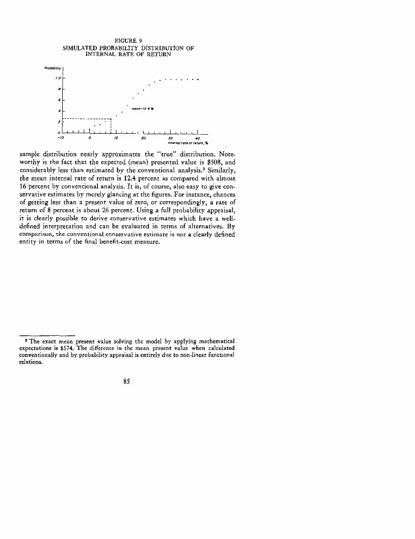
FIGURE 9SIMULATED PROBABILITY DISTRIBUTION OF

INTERNAL RATE OF RETURN

fProbab,/,t,

/0 - ,..... .

4 - /2 4

2 -------- -------

I I t I I I ! I , , , , I , , , , I . , , . I-/0 0 /0 20 30 40

/flttrfa/,ot. 0/f returin, %

sample distribution nearly approximates the "true" distribution. Note-worthy is the fact that the expected (mean) presented value is $508, andconsiderably less than estimated by the conventional analysis.3 Similarly,the mean internal rate of return is 12.4 percent as compared with almost16 percent by conventional analysis. It is, of course, also easy to give con-servative estimates by merely glancing at the figures. For instance, chancesof getting less than a present value of zero, or correspondingly, a rate ofreturn of 8 percent is about 26 percent. Using a full probability appraisal,it is clearly possible to derive conservative estimates which have a well-defined interpretation and can be evaluated in terms of alternatives. Bycomparison, the conventional conservative estimate is not a clearly defined

entity in terms of the final benefit-cost measure.

3 The exact mean present value solving the model by applying mathematicalexpectations is $574. The difference in the mean present value when calculatedconventionally and by probability appraisal is entirely due to non-linear functionalrelations.

85

ANNEX

REVIEW OF SOME BASIC CONCEPTS ANDRULES FROM PROBABILITY CALCULUS

WITH SPECIFIC APPLICATIONS

The concepts and rules discussed briefly in this annex should be primarilyuseful for deriving the mean and variance of a variable which is a functionof two or more other variables measured in terms of their probability dis-tributions.1 The presentation aims at providing a handy reference, not atmathematical rigor.

Some basic probability concepts

The problem-solving procedures for measuring the mean and variance ofthe present value of a stream of benefits from a project are specific applica-tions of a few general rules from the probability calculus. Hence, a briefreview of a few general rules are given below.2

1 As a useful reference, in terms of more mathematical rigor yet brief presenta-tion, the reader may consult R. V. Hogg and A. T. Craig, Introduction to Mathe-matical Statistics, Chapter 1 for probability and mathematical expectations con-cepts, and B. Wagle, "A Statistical Analysis of Risk in Capital Investment Proj-ects," Operations Research Quarterly, Vol. 18, No. I for special applications in riskappraisal. See also F. S. Hillier, "The Derivation of Probabilistic Information forthe Evaluation of Risky Investments," Management Science, Vol. 9, 1963.

2 For simplicity of representation, we shall discuss here only discrete probabilitydistribution.

87

First, let us define a probability distribution. Let all possible outcomesof an event be denoted by x,, i = 1 .... n, and let the probabilities ofeach outcome be denoted by p,, i.e.

f(x,) = p,

thenf(X) is a probability distribution if

Sp.= I

and (i=1. ,n)

pi 2 0In words, the probabilities must sum to one and negative probabilitie3 arenot admissible.

The concept of probability distribution can be generalized to two or mnorevariables. Let x, and y, be the outcomes of two events, and let the prob-ability of each joint outcome x,, y, be denoted by p,,, i.e.

f(xi,Yj) = pii (i = 1., n,j = 1., m)

thenf(X, Y) is a probability distribution if

ZP t , = 1

and (i = 1 .... , n, j = 1.,m)

pi, > 0

Mathematical expectations

One of the more useful concepts in problems involving probability distri-butions is that of a mathematical expectation. Let X be a set of events witha properly defined probability distributionf(X) and let g(X) be any functionof X, then the mathematical expectation E (or the expected value) ofg(X) is:

E[g(X)] = 5 p, g(xi) (i = 1 . , n)

For instance, if g(X) = X, then,

E(X) = p,x. ,n)

if g(X) = X2 , then

E(X2) = Ep.x2(i=1.

or if g(X) = (X + 4), then

E(X+ 4) = Ep1 (x. + 4) (i= 1 ... ,n)

88

The concept of mathematical expectations generalizes to two or more

variables. Let X and Y be sets of events with a properly defined probability

distribution, and let g(X, Y) be any function of X and Y, then the expecta-

tion of g(X, Y) is:

E[g(X, Y)] = p,, g(x,, y,)

(i = 1. n,j = 1. m)

For instance E(XY) is then,

E(XY) = 5Tp q xlyj (i = 1, .,n,j = 1, .,m)

Properties of mathematical expectations

Note the following properties of mathematical expectations:

(a) If k is a constant,

E(k) = k

(since E(k) = E p,k

= k ,p,, and 5pi = 1)

(b) If k is a constant and X is a variable,

E(kX) = k E(X)

(since E(kX) = Epikx, = k E p,x,)

(c) If ki and k2 are constants and X1 and X2 are variables

E(k,X, + k2x2) = k, E(XI) + k2 E(X2)

Special mathematical expectations

Some frequently used mathematical expectations are:

(A) The mean: E(X)

E(X) = pix,

(B) The variance: V(X) = E(X - E(X))2

V(X) = 7p, (xi - E(X))2

The variance can be computed by the formula:3

E(X 2) - (E(X))2 = Ep,X' 2 _ (p,X,) 2

3 The derivation is as follows:

E (X - E(X)) 2 = E[X 2 - 2E(X) X + (E(X)) 2]

= E(X2) - 2(E(X))2 + (E(X))2= E(X 2) - (E(X))2

89

(C) The covariance:4 cov. (XY) = E(X - E(X)) (Y - E(Y))

cov. (XY) = p,} (x, - E(X)) (y. - E(Y))

Making use of the properties of expectations, it can be showrt thatthe covariance is also

E(XY) - E(X) E(Y) = , p,x 1y, - paxi E p,yi

(D) The mean of a linear function:

If

Y = aX

then

E(Y) = aE(X)

(Note, therefore, that the mean of a linear function is a function ofthe mean. But the mean of a non-linear function is not a function ofthe mean, i.e. if Y = aX2 then E(Y) = aE(X2 ) and E(Y) #a(E(X))2

(E) The variance of a linear function:Similarly,

V(Y) = a2 V(X)

But if Y = aX2 , V(Y) = a2 V(X2 ) and V(Y) 5# a2 (V(X)) 2

(F) The mean of a sum: E(Y)

Given that Xi and X2 are random variables and a, and a2 areconstants, such that Y = a, X1 + a2 X2 , the mean of the sum is

E(Y) = a, E(X1) + a2 E(X2 )

(G) The variance of a sum:5 V(Y)

V(Y) = a12 V(X 1 ) + a22 V(X2 ) + 2 a, a2 cov. (X1 X2 )

4 Also, cov. (XY) = r V(X) v(Y), where r is the correlation coefficient.6 The variance of a sum can be derived as follows:

V(Y) = E[aiXi + a2X2 - a, E(X1 ) - a2 E(X2)12= E[a (XI -E(Xi)) + a2(X2 -E(X2))12= a

2 E(X -E(X 1))2 + a2 E(XI -E(X2))2

+ 2ala2 E[ (X - E(X)) (X 2 - E(X2 ))]

90

(H) The mean of a product if the covariance is zero:Note from (C) that if cov. (XY) = 0,

E(XY) = E(X) E(Y)

(I) The variance of a product if the covariance is zero:6

V(XY) = (E(X))2 V(Y) + (E(Y))2 V(X) + V(X) V(Y)

Special mathematical expectations useful in project appraisal

Assuming that the means of annual benefits are equal, let a' = (1 + r)-';t = 1, 2, .... , n, E(R) be the mean present value of a stream of benefits,and E(X) be the mean benefit in each year, then,

E(R) = (a + a2 + .... + an) E(X)

Assuming that the variance of annual benefits are equal, let V(R) be thevariance of the present value of a stream of benefits, V(X) be the varianceof the annual benefits, then if successive benefits are independent, i.e. allcovariances are zero,

V(R) = (a2 + a4 + .... + a2n) V(X)

if all successive benefits are perfectly correlated, i.e. cov. (X.,) = V(X)for i, j = 1, 2, .. , n, then,

V(R) = (a +a2 + ... an)2 V(X)

6 See L. A. Goodman, "On the Exact Variance of Products," Journal of AmericanStatistical Association, 1960.

91

ANNEX TABLE 1: Mean of Present Value, by Year and Interest Rate£ (t a'), t = 1, .,n, where a= (I - r)-

Number of Rate of Interest (r)Years

(n) 6% 8% 10%

1 0.9434 0.9259 0.90912 2.7234 2.6405 2.56193 5.2422 5.0219 4.81584 8.4106 7.9619 7.54785 12.1471 11.3649 10.65236 16.3771 15.1461 14.03937 21.0328 19.2306 17.63178 26.0520 23.5530 21.36379 31.3791 28.0548 25.1806

10 36.9631 32.6868 29.035611 42.7579 37.4047 32.891112 48.7219 42.1699 36.714313 54.8163 46.9500 40.480414 61.0085 51.7170 44.166615 67.2680 56.4450 47.757616 73.5656 61.1154 51.239217 79.8794 65.7105 54.601818 86.1848 70.2141 57.840019 92.4643 74.6164 60.946520 98.7003 78.9064 63.9185

92

ANNEX TABLE 2: Variance of Present Value, by Year and Interest Rate£ a2g, t = 1. ... Jn, where a (+ r) 1

Number of Rate of Interest (r)Years

(n) 6% 8% 10%

I .89000 .85734 .826452 1.68209 1.59237 1.509463 2.38705 2.22254 2.073934 3.01446 2.76281 2.540445 3.57285 3.22600 2.925986 4.06982 3.62311 3.244617 4.51212 3.96357 3.507948 4.90577 4.25546 3.725579 5.25611 4.50571 3.90543

10 5.56791 4.72026 4.0540711 5.84542 4.90420 4.1769212 6.09240 5.06190 4.2784513 6.31221 5.19710 4.3623614 6.50784 5.31301 4.4317015 6.68195 5.41239 4.4890116 6.83691 5.49759 4.5363717 6.97482 5.57064 4.5755118 7.09756 5.63326 4.6078619 7.20680 5.68695 4.6345920 7.30402 5.73298 4.6566821 7.39055 5.77244 4.6749422 7.46756 5.80627 4.6900323 7.53610 5.83528 4.7025024 7.59710 5.86015 4.7128125 7.65139 5.88147 4.7213326 7.69971 5.89975 4.7283727 7.74271 5.91542 4.7341928 7.78098 5.92886 4.7390029 7.81504 5.94038 4.7429730 7.84535 5.95026 4.74625

93

BIBLIOGRAPHY

Adelman, R. M. "Criteria for Capital Investment," Operational Research Quarterly,March 1965.

Arrow, K. J. "Alternative Approaches to the Theory of Choice in Risk-TakingSituations," Econometrica, Vol. 19, October 1951.

Arrow, K. J., T. Harris and J. Marshak. "Optimal Inventory Policy," Economctrica,Vol. 20, July 1951.

Bellman, R. Adaptive Control Processes: a Guided Tour. Princeton: Princetor Uni-versity Press, 1961.

Burt, 0. R. and D. R. Allison. "Farm Management Decisions with Dynamic Pro-gramming," Journal of Farm Economics, Vol. 45, 1963.

Dorfman, R. "Basic Economic and Technologic Concepts." Chapter in A. N4aaset al., Design of Water Resource Systems. Cambridge: Harvard University Ilress,1962.

Farrar, D. E. The Investment Decision Under Uncertainty. Englewood Cliffs, N.J.:Prentice-Hall, 1962.

Fellner, William. Probability and Profit. Homewood, Ill.: Richard D. Irwin, Inc.,1965.

Friedman, M. and L. T. Savage. "The Utility Analysis of Choice Involving Risk,"Journal of Political Economy, Vol. 56, August 1948.

Goodman, L. A. "On the Exact Variance of Products," Journal of American Sta-tistical Association, Vol. 55, 1960.

Hertz, 0. B. "Risk Analysis in Capital Investment," Harvard Business Review,January-February 1964.

Hillier, F. S. "The Derivation of Probabilistic Information for the Evaluation ofRisky Investments," Management Science, Vol. 9, 1963.

94

Hirshleifer, J. "Investment Decision Under Uncertainty: Applications of the State-Preference Approach," The Quarterly Journal of Economics, May 1966.

Hirshleifer, J. "Investment Decision Under Uncertainty: Choice-Theoretic Ap-proaches," The Quarterly Journal of Economics, Vol. 79, November 1965.

Howard, R. A. "Dynamic Inference," Operations Research, Vol. 13, September 1965.Lamberton, D. M. The Theory of Profit. Oxford: Basil Blackwell & Mott, Ltd., 1965.Maas, A. Design of Water Resource Systems. Cambridge: Harvard University Press,

1962.Markowitz, H. Portfolio Selection: Efficient Diversification of Investments. New York:

John Wiley & Sons, 1954.Marshak, J. "Money and the Theory of Assets," Econometrica, Vol. 6, 1938.Masse, Pierre. Optimal Investment Decisions, Englewood Cliffs, N.J.: Prentice-

Hall, 1962.Modigliani, F. and K. J. Cohen. "The Significance and Uses of Ex Ante Data."

Chapter IV in Expectations, Uncertainty and Business Behavior, edited by M. J.Bowman. New York: Social Science Research Council, 1958.

Orcutt, G. H. "Simulation of Economic Systems," American Economic Review,Vol. 50, 1961.

Ozga, S. Andrew. Expectations in Economic Theory, Chicago: Aldine PublishingCompany, 1965.

Pouliquen, L. Y. Risk Analysis in Project Appraisal, World Bank Staff OccasionalPaper No. 11.

Savage, L. J. The Foundations of Statistics. New York: John Wiley & Sons, 1954.Swalm, Ralph 0. "Utility Theory-Insights into Risk Taking," Harvard Business

Review, November-December 1966.von Neumann, J. and 0. Morgenstern. Theory of Games and Economic Behavior.

Princeton: Princeton University Press, 1947.Wagle, A. "A Statistical Analysis of Risk in Capital Investment Projects," Opera-

tional Research 9uarterly, Vol. 18, No. 1.Zusman, P. and A. Amaid. "Farm Planning under Weather Uncertainty," Journal

of Farm Economics, Vol. 14, August 1965.

95

EXPORT SALES REPRESENTATIVES

THE UNITED KINGDOM, CONTINENTAL EUROPE, THE NEAR EAST AND MIDDLE

EAST, AFRICA

The Johns Hopkins University Press, Ltd., 2-4 Brook Street, London

WIY-IAA, England

LATIN AMERICA AND THE CARIBBEAN

Unilibros, 5500 Ridge Oak Drive, Austin, Texas 78731, U.S.A.

AUSTRALIA, NEW ZEALAND, AND SOUTHEAST ASIA

Australia and New Zealand Book Co. Pty. Ltd., P.O. Box 459, Brookvale,

N.S.W. 2100, Australia

JAPAN

Maruzen Co., Ltd, P.O Box 5050, Tokyo International 100-31, Japan,

and bookstores of the Maruzen Co. throughout Japan

United Publishers Services Ltd., Shimura Building, 4-i Kojimachi,

Chiyoda-ku, Tokyo, Japan

CANADA

University of Toronto Press, Toronto, Canada M55 I A6

THROUGHOUT REST OF THE WORLD, orders can be sent directly to The Johns

Hopkins University Press, Baltimore, Maryland 21218, U.S.A

Published by The Johns Hopkins University Press

Baltzmore and London

go THE WORLD BANK

Other World Bank booksof related interest from Johns Hopkins

METHODS OF PROJECT ANALYSIS: A REVIEWDeepak LalISBN 0-8018-1615-7, paperback

RISK ANALYSIS IN PROJECT APPRAISALLouis Y. PouliquenISBN 0-8018-1155-4, paperback

ECONOMIC ANALYSIS OF PROJECTSLyn Squire and Herman G. van der TakISBN 0-8018-1817-6, clothbound; ISBN 0-8018-1818-4, paperback

The Johns Hopkins University Press Baltimore and London

ISBN 0-8018-1154-6 Cover design by Carol Crosby Black