Embed Size (px)
Citation preview
Sawyer, D.S., Whitmarsh, R.B., Klaus, A., et al., 1994 Proceedings of the Ocean Drilling Program, Initial Reports, Vol. 149
2. EXPLANATORY NOTES1
Shipboard Scientific Party2
INTRODUCTION
In this chapter, we have assembled information that will help the reader to understand the observations on which our preliminary con- clusions have been based and also help the interested investigator to select samples for further analysis. This information concerns only shipboard operations and analyses described in the site reports in the Initial Reports volume of the Leg 149 Proceedings of the Ocean Drilling Program. Methods used by various investigators for shore- based analyses of Leg 149 data will be described in the individual sci- entific contributions to be published in the Scientific Results volume.
Authorship of Site Chapters
The separate sections of the site chapters were written by the fol- lowing shipboard scientists (authors are listed in alphabetical order, no seniority is implied):
Site Summary: Sawyer, Whitmarsh Background and Objectives: Sawyer, Whitmarsh Operations: Pollard, Klaus Site Geophysics: Sawyer, Whitmarsh Lithostratigraphy: Comas, Marsaglia, Milkert, Milliken, Ra-
mirez, Wilson Biostratigraphy: Collins, Gervais, de Kaenel, Liu Paleomagnetism: Kanamatsu, Zhao Igneous and Metamorphic Petrology and Geochemistry: Beslier,
Cornen, Gibson, Seifert Structural Geology: Beslier, Morgan Organic Geochemistry: Meyers Inorganic Geochemistry: Shaw Physical Properties: Harry, Krawczyk, Morgan, Pinheiro Downhole Measurements: Hobart, Lofts, Yin Integration of Seismic Profiles with Observations from the Site:
Whitmarsh Downhole Temperature Measurements: Harry, Hobart, Sawyer Summary and Conclusions: Sawyer, Whitmarsh
Following the text of all the site chapters, summary core descrip- tions ("barrel sheets") and photographs of each core are presented in a section called "Cores."
Drilling Characteristics
Core handling and shipboard scientific procedures, including the numbering of sites, holes, cores, sections, and samples were similar to those reported in previous Initial Reports volumes of the Proceed- ings of the Ocean Drilling Program (Shipboard Scientific Party, 1993c). Procedures for handling of igneous rock are similar to those used for Leg 147 (Shipboard Scientific Party, 1993a).
1Sawyer, D.S., Whitmarsh, R.B., Klaus, A., et al., 1994. Proc. ODP, Init. Repts., 149: College Station, TX (Ocean Drilling Program).
2Shipboard Scientific Party is as given in list of participants preceding the contents.
Reproduced online: 15 October 2004.
At the end of the leg, the cores were transferred from the ship in refrigerated airfreight containers to cold storage at the East Coast Re- pository of the Ocean Drilling Program, at the Lamont-Doherty Earth Observatory, Columbia University, New York.
LITHOSTRATIGRAPHY
The first part of this section summarizes the methods used to de- scribe sediment cores and the manner in which data collected manu- ally for visual core description forms (VCDs) are summarized and condensed into computer-generated summaries for each core. The second part reviews the sedimentological classifications and terms used in the descriptions.
Visual Core Descriptions (VCDs) of Sedimentary Units Core Description Forms
Shipboard sedimentologists were responsible for visual core log- ging, smear-slide analyses, and thin-section descriptions of sedimen- tary and volcaniclastic material. During Leg 149, information recorded section-by-section on VCD sheets was condensed onto computer-generated summaries that give graphic and textual summa- ries for each core (see "Cores" section, this volume).
Cores were designated using leg number, site number, hole letter, core number, and core type, as discussed in Shipboard Scientific Par- ty (1993c). The cored interval was specified in terms of meters below sea level (mbsl) and meters below seafloor (mbsf). On the basis of drill-pipe measurements (dpm), reported by the SEDCO Coring Technician and the ODP Operations Superintendent, depths were corrected for the height of the rigfloor dual elevator stool above sea level to give true water depth and correct depth below sea level.
"Graphic Lithology" Column
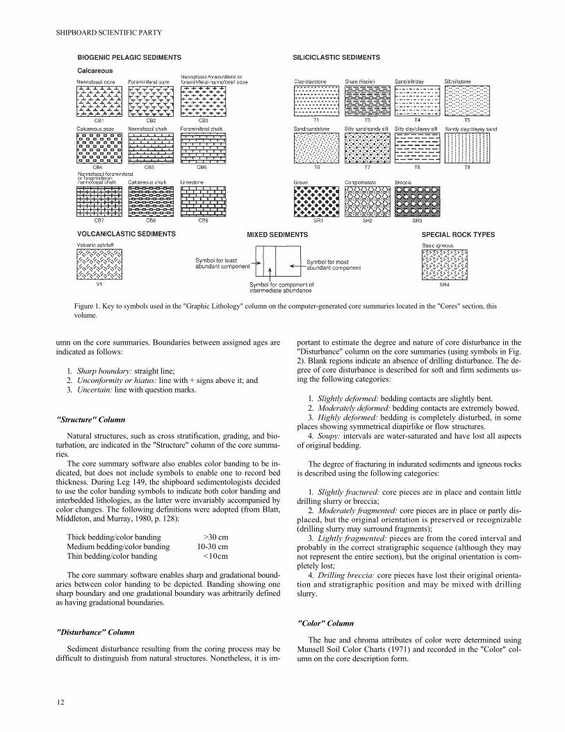
The lithology of the recovered material is represented on the com- puter-generated core description forms by symbols representing as many as three components in the column titled "Graphic Lithology" (see bottom right of Fig. 1). Constituents accounting for < 10% of the sediment in a given lithology (or others remaining after the represen- tation of the three most abundant lithologies) are not shown in the "Graphic Lithology" column, but are listed in the "Lithologic De- scription" section of the core description form. Because of the limi- tations of the software used for generating the core summaries, the "Graphic Lithology" column shows only the composition of layers or intervals exceeding 20 cm in thickness. This meant that the VCDs for Leg 149 often do not show the nature of vertical changes in the cores, as many of the repetitive sequences present are less than 20 cm thick.
"Age" Column
The chronostratigraphic unit, as recognized on the basis of pale- ontological and paleomagnetic criteria, is shown in the "Age" col-
11
SHIPBOARD SCIENTIFIC PARTY
12
Figure 1. Key to symbols used in the "Graphic Lithology" column on the computer-generated core summaries located in the "Cores" section, this volume.
umn on the core summaries. Boundaries between assigned ages are indicated as follows:
1. Sharp boundary: straight line; 2. Unconformity or hiatus: line with + signs above it; and 3. Uncertain: line with question marks.
"Structure" Column
Natural structures, such as cross stratification, grading, and bio- turbation, are indicated in the "Structure" column of the core summa- ries.
The core summary software also enables color banding to be in- dicated, but does not include symbols to enable one to record bed thickness. During Leg 149, the shipboard sedimentologists decided to use the color banding symbols to indicate both color banding and interbedded lithologies, as the latter were invariably accompanied by color changes. The following definitions were adopted (from Blatt, Middleton, and Murray, 1980, p. 128):
Thick bedding/color banding >30 cm Medium bedding/color banding 10-30 cm Thin bedding/color banding <10cm
The core summary software enables sharp and gradational bound- aries between color banding to be depicted. Banding showing one sharp boundary and one gradational boundary was arbitrarily defined as having gradational boundaries.
"Disturbance" Column
Sediment disturbance resulting from the coring process may be difficult to distinguish from natural structures. Nonetheless, it is im-
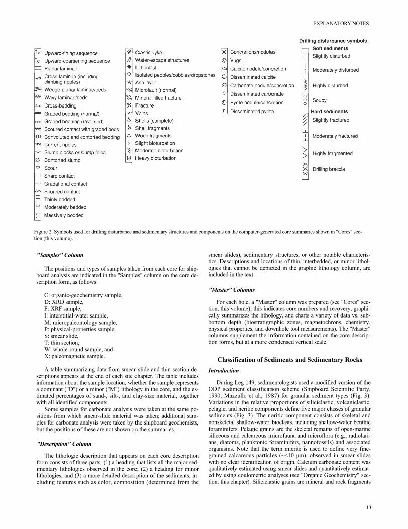
portant to estimate the degree and nature of core disturbance in the "Disturbance" column on the core summaries (using symbols in Fig. 2). Blank regions indicate an absence of drilling disturbance. The de- gree of core disturbance is described for soft and firm sediments us- ing the following categories:
1. Slightly deformed: bedding contacts are slightly bent. 2. Moderately deformed: bedding contacts are extremely bowed. 3. Highly deformed: bedding is completely disturbed, in some
places showing symmetrical diapirlike or flow structures. 4. Soupy: intervals are water-saturated and have lost all aspects
of original bedding.
The degree of fracturing in indurated sediments and igneous rocks is described using the following categories:
1. Slightly fractured: core pieces are in place and contain little drilling slurry or breccia;
2. Moderately fragmented: core pieces are in place or partly dis- placed, but the original orientation is preserved or recognizable (drilling slurry may surround fragments);
3. Lightly fragmented: pieces are from the cored interval and probably in the correct stratigraphic sequence (although they may not represent the entire section), but the original orientation is com- pletely lost;
4. Drilling breccia: core pieces have lost their original orienta- tion and stratigraphic position and may be mixed with drilling slurry.
"Color" Column
The hue and chroma attributes of color were determined using Munsell Soil Color Charts (1971) and recorded in the "Color" col- umn on the core description form.
EXPLANATORY NOTES
Figure 2. Symbols used for drilling disturbance and sedimentary structures and components on the computer-generated core summaries shown in "Cores" sec- tion (this volume).
"Samples" Column
The positions and types of samples taken from each core for ship- board analysis are indicated in the "Samples" column on the core de- scription form, as follows:
C: organic-geochemistry sample, D: XRD sample, F: XRF sample, I: interstitial-water sample, M: micropaleontology sample, P: physical-properties sample, S: smear slide, T: thin section, W: whole-round sample, and X: paleomagnetic sample.
A table summarizing data from smear slide and thin section de- scriptions appears at the end of each site chapter. The table includes information about the sample location, whether the sample represents a dominant ("D") or a minor ("M") lithology in the core, and the es- timated percentages of sand-, silt-, and clay-size material, together with all identified components.
Some samples for carbonate analysis were taken at the same po- sitions from which smear-slide material was taken; additional sam- ples for carbonate analysis were taken by the shipboard geochemists, but the positions of these are not shown on the summaries.
"Description" Column
The lithologic description that appears on each core description form consists of three parts: (1) a heading that lists all the major sed- imentary lithologies observed in the core; (2) a heading for minor lithologies, and (3) a more detailed description of the sediments, in- cluding features such as color, composition (determined from the
smear slides), sedimentary structures, or other notable characteris- tics. Descriptions and locations of thin, interbedded, or minor lithol- ogies that cannot be depicted in the graphic lithology column, are included in the text.
"Master" Columns
For each hole, a "Master" column was prepared (see "Cores" sec- tion, this volume); this indicates core numbers and recovery, graphi- cally summarizes the lithology, and charts a variety of data vs. sub- bottom depth (biostratigraphic zones, magnetochrons, chemistry, physical properties, and downhole tool measurements). The "Master" columns supplement the information contained on the core descrip- tion forms, but at a more condensed vertical scale.
Classification of Sediments and Sedimentary Rocks Introduction
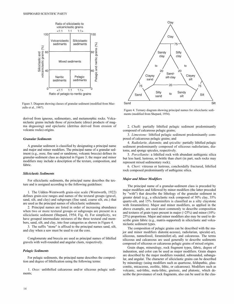
During Leg 149, sedimentologists used a modified version of the ODP sediment classification scheme (Shipboard Scientific Party, 1990; Mazzullo et al., 1987) for granular sediment types (Fig. 3). Variations in the relative proportions of siliciclastic, volcaniclastic, pelagic, and neritic components define five major classes of granular sediments (Fig. 3). The neritic component consists of skeletal and nonskeletal shallow-water bioclasts, including shallow-water benthic foraminifers. Pelagic grains are the skeletal remains of open-marine siliceous and calcareous microfauna and microflora (e.g., radiolari- ans, diatoms, planktonic foraminifers, nannofossils) and associated organisms. Note that the term micrite is used to define very fine- grained calcareous particles (~<10 µm), observed in smear slides with no clear identification of origin. Calcium carbonate content was qualitatively estimated using smear slides and quantitatively estimat- ed by using coulometric analyses (see "Organic Geochemistry" sec- tion, this chapter). Siliciclastic grains are mineral and rock fragments
13
SHIPBOARD SCIENTIFIC PARTY
Fz
igure 3. Diagram showing classes of granular sediment (modified from Maz- ullo et al., 1987).
derived from igneous, sedimentary, and metamorphic rocks. Volca- niclastic grains include those of pyroclastic (direct products of mag- ma degassing) and epiclastic (detritus derived from erosion of volcanic rocks) origins.
Granular Sediments
A granular sediment is classified by designating a principal name and major and minor modifiers. The principal name of a granular sed- iment (e.g., ooze, fine sand or sandstone, volcanic breccia) defines its granular-sediment class as depicted in Figure 3; the major and minor modifiers may include a description of the texture, composition, and fabric.
Siliciclastic Sediments
For siliciclastic sediments, the principal name describes the tex- ture and is assigned according to the following guidelines:
1. The Udden-Wentworth grain-size scale (Wentworth, 1922) defines grain-size ranges and names of the textural groups (gravel, sand, silt, and clay) and subgroups (fine sand, coarse silt, etc.) that are used as the principal names of siliciclastic sediments.
2. Principal names are listed in order of increasing abundance when two or more textural groups or subgroups are present in a siliciclastic sediment (Shepard, 1954; Fig. 4). For simplicity, we have grouped intermediate mixtures of the three textural end mem- bers, sand, silt, and clay, into four categories as shown in Figure 4.
3. The suffix "stone" is affixed to the principal names sand, silt, and clay when a saw must be used to cut the core.
Conglomerate and breccia are used as principal names of lithified gravels with well-rounded and angular clasts, respectively.
Pelagic Sediments
For pelagic sediments, the principal name describes the composi- tion and degree of lithification using the following terms:
1. Ooze: unlithified calcareous and/or siliceous pelagic sedi- ments;
14
Figure 4. Ternary diagram showing principal names for siliciclastic sedi- ments (modified from Shepard, 1954).
2. Chalk: partially lithified pelagic sediment predominantly composed of calcareous pelagic grains;
3. Limestone: lithified pelagic sediment predominantly com- posed of calcareous pelagic grains; and
4. Radiolarite, diatomite, and spiculite: partially lithified pelagic sediment predominantly composed of siliceous radiolarians, dia- toms, and sponge spicules, respectively.
5. Porcellanite: a lithified rock with abundant authigenic silica but less hard, lustrous, or brittle than chert (in part, such rocks may represent mixed sedimentary rock);
6. Chert: vitreous or lustrous, conchoidally fractured, lithified rock composed predominantly of authigenic silica.
Major and Minor Modifiers
The principal name of a granular-sediment class is preceded by major modifiers and followed by minor modifiers (the latter preceded by "with") that describe the lithology of the granular sediment in greater detail (e.g., a siliciclastic rock composed of 50% clay, 35% quartz-silt, and 15% foraminifers is classified as a silty claystone with foraminifers). Major and minor modifiers, as applied in the above example, are used most commonly to describe composition and textures of grain types present in major (>25%) and minor (10%- 25%) proportions. Major and minor modifiers also may be used to de- scribe grain fabric (e.g., matrix-supported) in siliciclastic and volca- niclastic sediment types.
The composition of pelagic grains can be described with the ma- jor and minor modifiers diatom(-aceous), radiolarian, spicule(-ar), siliceous, nannofossil, foraminifer(-al), and calcareous. The terms siliceous and calcareous are used generally to describe sediments composed of siliceous or calcareous pelagic grains of mixed origins.
Grain shape, mineralogy, rock fragment types, fabric, degree of induration, and color can be used as major modifiers. Grain shapes are described by the major modifiers rounded, subrounded, subangu- lar, and angular. The character of siliciclastic grains can be described by mineralogy (using modifiers such as quartzose, feldspathic, glau- conitic, micaceous, zeolitic, lithic, or calcareous). Modifiers such as volcanic, sed-lithic, meta-lithic, gneissic, and plutonic, which de- scribe the provenance of rock fragments, also can be used in the clas-
EXPLANATORY NOTES
sification of sediments (particularly in gravels, conglomerates, and breccias). The fabric of a sediment can be described as well using ma- jor modifiers such as grain-supported, matrix-supported, and imbri- cated. Generally, fabric terms are useful only when describing gravels, conglomerates, and breccias. The degree of lithification is described using the following major modifiers: "unlithified" desig- nates soft sediment that is readily deformable by finger pressure, "partially lithified" designates firm sediment that is incompletely lithified, and "lithified" designates hard, cemented sediment that must be cut with a saw. Finally, sediment color, as determined visu- ally with the Munsell Soil Color Chart (1971), also can be employed as a major modifier.
Mixed sediments are described using major and minor modifiers indicating composition and texture.
X-ray Diffraction Methods for Fine Fractions
The fine fraction of selected samples was analyzed on board the ship using X-ray diffraction techniques. Sediments were put into sus- pension by ultrasonic disaggregation, and the fine fraction (<1 µm) was separated by centrifuging and then used to prepare air-dried specimens on glass slides. X-ray diffraction patterns of these oriented specimens were produced using the shipboard Philips AD 3420 X- ray diffractometer (CuK alpha emission source). Selected samples were treated with ethyleneglycol and re-analyzed. Other selected samples were heated at 550°C for 1 to 1.5 hr, and then reanalyzed. Peaks were visually inspected and matched to standard reference peaks for various minerals (quartz, feldspar, hornblende, calcite, py- rite, and clay minerals, etc.).
BIOSTRATIGRAPHY
Preliminary age assignments were established using core-catcher samples. Samples from elsewhere in the cores were examined when a more refined age determination was necessary. Two microfossil groups were examined for biostratigraphic purposes: calcareous nan- nofossils and planktonic foraminifers. Benthic foraminifers were used to estimate paleobathymetry. Sample positions and the abun- dance, preservation, and age or zone for each fossil group were re- corded on barrel sheets for each core.
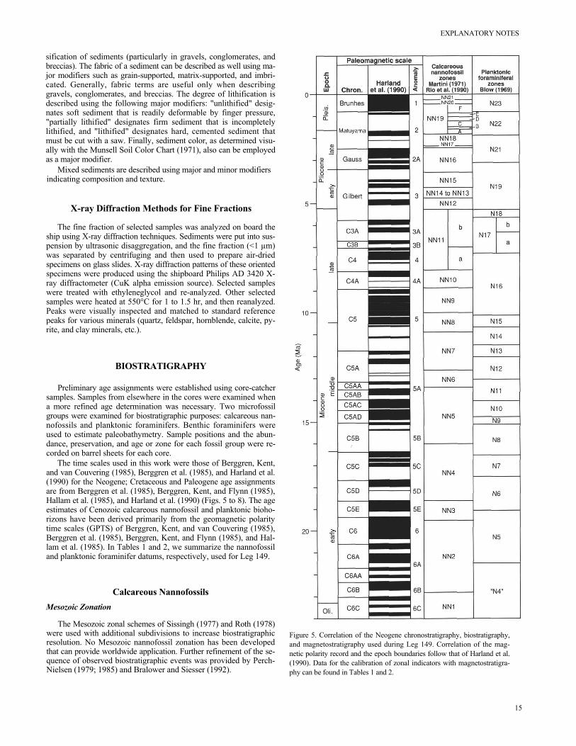
The time scales used in this work were those of Berggren, Kent, and van Couvering (1985), Berggren et al. (1985), and Harland et al. (1990) for the Neogene; Cretaceous and Paleogene age assignments are from Berggren et al. (1985), Berggren, Kent, and Flynn (1985), Hallam et al. (1985), and Harland et al. (1990) (Figs. 5 to 8). The age estimates of Cenozoic calcareous nannofossil and planktonic bioho- rizons have been derived primarily from the geomagnetic polarity time scales (GPTS) of Berggren, Kent, and van Couvering (1985), Berggren et al. (1985), Berggren, Kent, and Flynn (1985), and Hal- lam et al. (1985). In Tables 1 and 2, we summarize the nannofossil and planktonic foraminifer datums, respectively, used for Leg 149.
Calcareous Nannofossils Mesozoic Zonation
The Mesozoic zonal schemes of Sissingh (1977) and Roth (1978) were used with additional subdivisions to increase biostratigraphic resolution. No Mesozoic nannofossil zonation has been developed that can provide worldwide application. Further refinement of the se- quence of observed biostratigraphic events was provided by Perch- Nielsen (1979; 1985) and Bralower and Siesser (1992).
Figure 5. Correlation of the Neogene chronostratigraphy, biostratigraphy, and magnetostratigraphy used during Leg 149. Correlation of the mag- netic polarity record and the epoch boundaries follow that of Harland et al. (1990). Data for the calibration of zonal indicators with magnetostratigra- phy can be found in Tables 1 and 2.
15
SHIPBOARD SCIENTIFIC PARTY
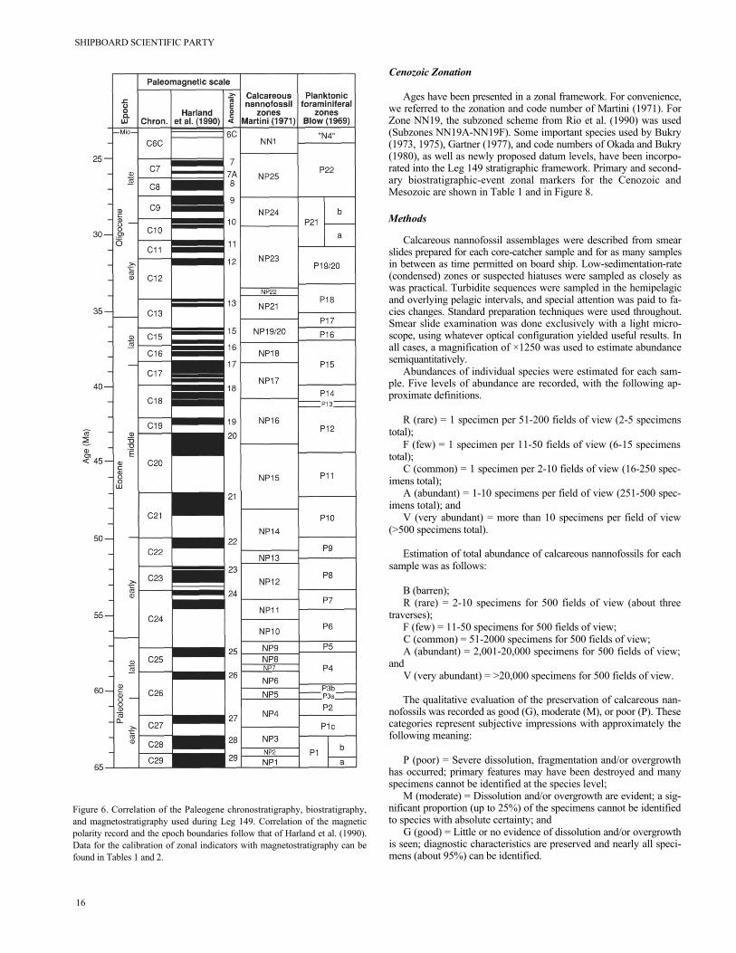
Figure 6. Correlation of the Paleogene chronostratigraphy, biostratigraphy, and magnetostratigraphy used during Leg 149. Correlation of the magnetic polarity record and the epoch boundaries follow that of Harland et al. (1990). Data for the calibration of zonal indicators with magnetostratigraphy can be found in Tables 1 and 2.
16
Cenozoic Zonation
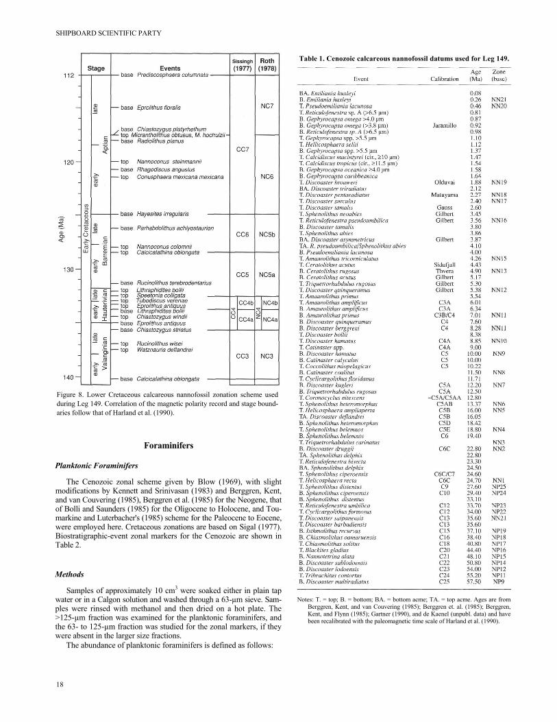
Ages have been presented in a zonal framework. For convenience, we referred to the zonation and code number of Martini (1971). For Zone NN19, the subzoned scheme from Rio et al. (1990) was used (Subzones NN19A-NN19F). Some important species used by Bukry (1973, 1975), Gartner (1977), and code numbers of Okada and Bukry (1980), as well as newly proposed datum levels, have been incorpo- rated into the Leg 149 stratigraphic framework. Primary and second- ary biostratigraphic-event zonal markers for the Cenozoic and Mesozoic are shown in Table 1 and in Figure 8.
Methods
Calcareous nannofossil assemblages were described from smear slides prepared for each core-catcher sample and for as many samples in between as time permitted on board ship. Low-sedimentation-rate (condensed) zones or suspected hiatuses were sampled as closely as was practical. Turbidite sequences were sampled in the hemipelagic and overlying pelagic intervals, and special attention was paid to fa- cies changes. Standard preparation techniques were used throughout. Smear slide examination was done exclusively with a light micro- scope, using whatever optical configuration yielded useful results. In all cases, a magnification of ×1250 was used to estimate abundance semiquantitatively.
Abundances of individual species were estimated for each sam- ple. Five levels of abundance are recorded, with the following ap- proximate definitions.
R (rare) = 1 specimen per 51-200 fields of view (2-5 specimens total);
F (few) = 1 specimen per 11-50 fields of view (6-15 specimens total);
C (common) = 1 specimen per 2-10 fields of view (16-250 spec- imens total);
A (abundant) = 1-10 specimens per field of view (251-500 spec- imens total); and
V (very abundant) = more than 10 specimens per field of view (>500 specimens total).
Estimation of total abundance of calcareous nannofossils for each sample was as follows:
B (barren); R (rare) = 2-10 specimens for 500 fields of view (about three
traverses); F (few) = 11-50 specimens for 500 fields of view; C (common) = 51-2000 specimens for 500 fields of view; A (abundant) = 2,001-20,000 specimens for 500 fields of view;
and V (very abundant) = >20,000 specimens for 500 fields of view.
The qualitative evaluation of the preservation of calcareous nan- nofossils was recorded as good (G), moderate (M), or poor (P). These categories represent subjective impressions with approximately the following meaning:
P (poor) = Severe dissolution, fragmentation and/or overgrowth has occurred; primary features may have been destroyed and many specimens cannot be identified at the species level;
M (moderate) = Dissolution and/or overgrowth are evident; a sig- nificant proportion (up to 25%) of the specimens cannot be identified to species with absolute certainty; and
G (good) = Little or no evidence of dissolution and/or overgrowth is seen; diagnostic characteristics are preserved and nearly all speci- mens (about 95%) can be identified.
EXPLANATORY NOTES
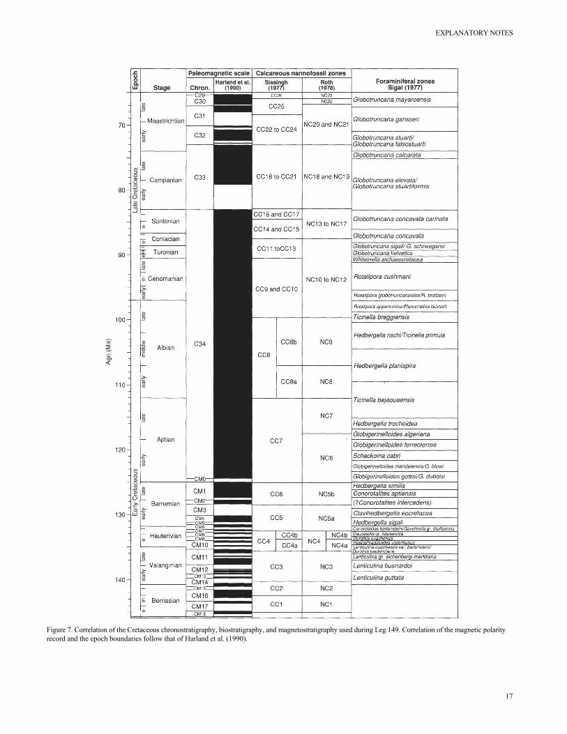
Figure 7. Correlation of the Cretaceous chronostratigraphy, biostratigraphy, and magnetostratigraphy used during Leg 149. Correlation of the magnetic polarity
record and the epoch boundaries follow that of Harland et al. (1990).17
SHIPBOARD SCIENTIFIC PARTY
Figure 8. Lower Cretaceous calcareous nannofossil zonation scheme used during Leg 149. Correlation of the magnetic polarity record and stage bound- aries follow that of Harland et al. (1990).
Foraminifers
Planktonic Foraminifers
The Cenozoic zonal scheme given by Blow (1969), with slight modifications by Kennett and Srinivasan (1983) and Berggren, Kent, and van Couvering (1985), Berggren et al. (1985) for the Neogene, that of Bolli and Saunders (1985) for the Oligocene to Holocene, and Tou- markine and Luterbacher's (1985) scheme for the Paleocene to Eocene, were employed here. Cretaceous zonations are based on Sigal (1977). Biostratigraphic-event zonal markers for the Cenozoic are shown in Table 2.
Methods
Samples of approximately 10 cm3 were soaked either in plain tap water or in a Calgon solution and washed through a 63-µm sieve. Sam- ples were rinsed with methanol and then dried on a hot plate. The >125-µm fraction was examined for the planktonic foraminifers, and the 63- to 125-µm fraction was studied for the zonal markers, if they were absent in the larger size fractions.
The abundance of planktonic foraminifers is defined as follows:
18
Table 1. Cenozoic calcareous nannofossil datums used for Leg 149.
Notes: T. = top; B. = bottom; BA. = bottom acme; TA. = top acme. Ages are from
Berggren, Kent, and van Couvering (1985); Berggren et. al. (1985); Berggren, Kent, and Flynn (1985); Gartner (1990), and de Kaenel (unpubl. data) and have been recalibrated with the paleomagnetic time scale of Harland et al. (1990).
EXPLANATORY NOTES
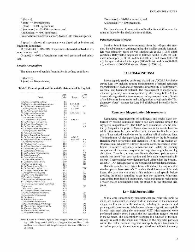
B (barren); R (rare) = <10 specimens; F (few) = 10-100 specimens; C (common) = 101-500 specimens; and A (abundant) = >500 specimens. Preservation characteristics were divided into three categories:
P (poor) = almost all specimens were dissolved or broken and fragments dominated;
M (moderate) = 30%-90% of specimens showed dissolved or bro- ken chambers; and
G (good) = >90% of specimens were well preserved and unbro- ken.
Benthic Foraminifers
The abundance of benthic foraminifers is defined as follows:
B (barren); R (rare) = <10 specimens;
Table 2. Cenozoic planktonic foraminifer datums used for Leg 149.
Notes: T. = top; B. = bottom. Ages are from Berggren, Kent, and van Couver-
ing (1985), Berggren et al. (1985), and Berggren, Kent, and Flynn (1985) and have been calibrated with the paleomagnetic time scale of Harland et al. (1990).
C (common) = 10-100 specimens; and A (abundant) = > 100 specimens.
The three classes of preservation of benthic foraminifers were the same as those for the planktonic foraminifers.
Paleobathymetric Methods
Benthic foraminifers were examined from the >63-µm size frac- tion. Paleobathymetry estimated using the smaller benthic foramini- fers was primarily based on van Morkhoven et al.'s (1986) depth zonations. Bathymetric ranges are as follows: neritic (0-200 m) is di- vided into upper (0-30 m), middle (30-100 m), and lower (100-200 m); bathyal is divided into upper (200-600 m), middle (600-1000 m), and lower (1000-2000 m); and abyssal (>2000 m).
PALEOMAGNETISM
Paleomagnetic studies performed aboard the JOIDES Resolution during Leg 149 included routine measurements of natural remanent magnetization (NRM) and of magnetic susceptibility of sedimentary, volcanic, and basement material. The measurement of magnetic re- manence generally was accompanied by alternating field (AF) or thermal demagnetization to remove secondary magnetization. Details of the laboratory instruments and configurations are given in the "Ex- planatory Notes" chapter for Leg 145 (Shipboard Scientific Party, 1993c).
Remanent Magnetization Measurements
Remanence measurements of sediments and rocks were per- formed by passing continuous archive-half core sections through the cryogenic magnetometer. The ODP core orientation scheme arbi- trarily designates the positive X-axis direction as the in-situ horizon- tal direction from the center of the core to the median line between a pair of lines scribed lengthwise on the working half of each core liner. The maximum AF demagnetizing field allowed by the Information Handling Panel for archive-half sections is 15 mT or the median de- structive field, whichever is lower. In some cores, this field is insuf- ficient to remove secondary remanence and isolate the primary component of remanence required for magnetostratigraphy and leg objectives. Therefore, at least one discrete shipboard paleomagnetic sample was taken from each section and from each representative li- thology. These samples were demagnetized using either the Schonst- edt GSD-1 AF demagnetizer or the Schonstedt thermal demagnetizer.
Discrete samples were taken from soft sediment using oriented standard plastic boxes (6 cm3). To reduce the deformation of the sed- iment, the core was cut using a thin stainless steel spatula before pressing the plastic sampling boxes into the sediment. Minicores were drilled from lithified sedimentary rocks and igneous rocks using a water-cooled nonmagnetic drill bit attached to the standard drill press.
Low-field Susceptibility
Whole-core susceptibility measurements are relatively rapid to make, are nondestructive, and provide an indication of the amount of magnetizable material in the sediment, including ferrimagnetic and paramagnetic constituents. Whole-core volume magnetic susceptibil- ity was measured using the automated MST. Measurements were performed usually every 5 cm at the low sensitivity range (1.0) and in the SI mode. The susceptibility response is a function of the min- eralogy as well as the shape and volume of the magnetic particles within the rocks. Because magnetic susceptibility is a temperature- dependent property, the cores were permitted to equilibrate thermally
19
SHIPBOARD SCIENTIFIC PARTY
(2-4 hr) prior to measurement. The general trend of the susceptibility curve was used to characterize both the magnetic material in the sed- iment cores, as well as subtle environmental and geologic changes within the sediments.
Core Orientation
Core orientation of the advanced hydraulic piston (APC) cores was achieved with an Eastman-Whipstock multishot tool and the new Tensor multishot tool, both of which are rigidly mounted on a non- magnetic sinker bar. The Eastman-Whipstock tool consists of a mag- netic compass and a small camera. The battery-operated camera takes photographs at prescribed intervals from 0.5 to 2 min from the time it leaves the deck. At the bottom of the hole, the core barrel is allowed to rest for sufficient time (2-8 min) to permit the compass needle to settle and to make sure that several photographs are taken before the corer is shot into the sediment.
The Tensor tool consists of three mutually perpendicular magnet- ic sensors and two perpendicular gimbals. The information from both sets of sensors allows the azimuth and dip of the hole to be measured, as well as the azimuth of the double orientation line on the core liner.
Magnetostratigraphy
Where magnetic cleaning successfully isolates the primary com- ponent of remanence, paleomagnetic inclinations are used to assign a magnetic polarity to the stratigraphic column. With the assistance of biostratigraphic data, we attempted an interpretation of the magnetic polarity stratigraphy in the site chapters. During Leg 149, we adhered to the chronostratigraphic nomenclature and geochronology of Har- land et al. (1990; see Table 3 and Figs. 5 to 7). For the Neogene, we used the revised ages of geomagnetic reversal boundaries taken from the new magnetic polarity time scale of Cande and Kent (1992).
IGNEOUS AND METAMORPHIC PETROLOGY AND GEOCHEMISTRY
Core Curation and Shipboard Sampling
Before splitting igneous and metamorphic rock cores, the whole cores were examined for structural features. Sediments in contact with the hard rocks were examined for evidence of chilling, baking, and alteration. Contiguous pieces of core were numbered sequential- ly from the top of each core section and labeled according to standard ODP procedures. Cores were split in such a way as to allow important features and structures to be represented in both the working and ar- chive samples. The archive half was described on the visual core de- scription (VCD) form and was photographed before storage. Only the working half was sampled.
Visual Core Descriptions of Igneous Rocks
The standard visual core description forms were used to document the location of samples taken from the igneous rock cores (see "Cores" section, this volume) using the following notation: XRD = X-ray diffraction analysis; XRF = X-ray fluorescence analysis; TSB = petrographic thin section. When describing sequences of rocks, the core was subdivided into lithologic units on the basis of changes in texture, grain size, mineral occurrence and abundance, rock compo- sition, and rock clast type. Rocks for which the protolith is complete- ly obscured by metamorphism were given separate lithological names, whereas the prefix "meta" or the term "altered" is used as a modifier with the name of an identifiable protolith. We reserved the termed "altered" for igneous rocks that contain only those secondary
20
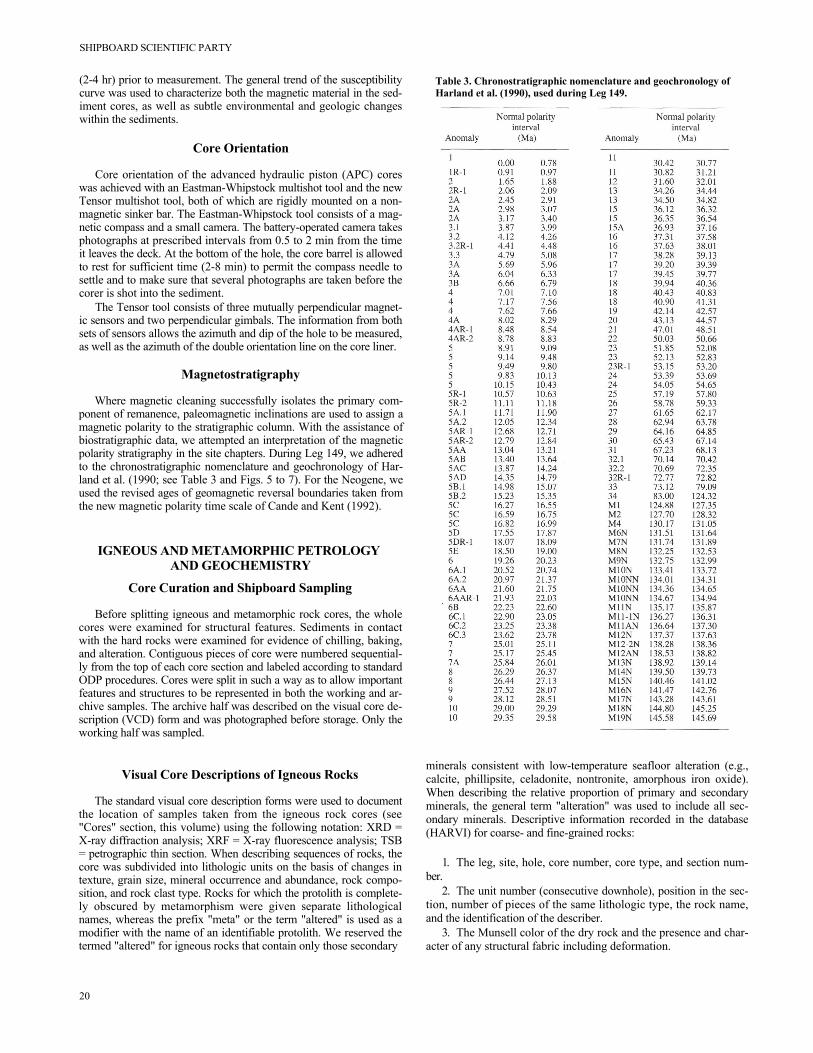
Table 3. Chronostratigraphic nomenclature and geochronology of Harland et al. (1990), used during Leg 149.
minerals consistent with low-temperature seafloor alteration (e.g., calcite, phillipsite, celadonite, nontronite, amorphous iron oxide). When describing the relative proportion of primary and secondary minerals, the general term "alteration" was used to include all sec- ondary minerals. Descriptive information recorded in the database (HARVI) for coarse- and fine-grained rocks:
1. The leg, site, hole, core number, core type, and section num- ber.
2. The unit number (consecutive downhole), position in the sec- tion, number of pieces of the same lithologic type, the rock name, and the identification of the describer.
3. The Munsell color of the dry rock and the presence and char- acter of any structural fabric including deformation.
EXPLANATORY NOTES
4. The number of mineral phases visible with a hand lens and their distribution within the unit, together with the following infor- mation for each phase: (a) abundance (volume %); (b) size range in mm; (c) shape; (d) degree of alteration; and (e) further comments.
5. The groundmass texture: glassy, fine grained (<1 mm), medium grained (1-5 mm), or coarse grained (>5 mm). Grain size changes within units were also noted.
6. The presence and characteristics of secondary minerals and alteration products.
7. The relative amount of rock alteration was described in the rock description. Rocks were classified as fresh (<2%); slightly altered (2%-10%); moderately altered (10%-40%); highly altered (40%-80%); very highly altered (80%-95%); and completely altered (95%-100%). The type, form, and distribution of alteration was also noted.
8. The presence of veins and fractures, including their abun- dance, width, mineral fillings or coatings, orientation, and associated wall rock alteration. The hade of veins and fractures with respect to the core axis was measured with a protractor (see "Structural Geol- ogy" section, this chapter). The relationship of the alteration and vein filling minerals with respect to veins and fractures also was noted. Vein networks and their mineralogy were indicated adjacent to the graphic representation of the archive half.
9. Other comments, including notes on the continuity of the unit within the core and on the interrelationship of units.
Fine-grained Volcanic Rocks
Basalt is called aphyric (<1%), sparsely phyric (1%-2%), moder- ately phyric (2%-10%), or highly phyric (>10%), depending upon the proportion of phenocrysts visible with the hand lens and binocu- lar microscope. Basalts are further described by phenocryst type (e.g., a moderately plagioclase-olivine phyric basalt contains 2%- 10% phenocrysts, mostly plagioclase, with subordinate olivine). The abundance of vesicles, their shape, and type of mineral fillings were also noted. More specific rock names were given where chemical analyses or thin sections were available.
Brecciated Rocks
A breccia is defined as any rock composed of angular broken rock fragments held together by finer fragments or glassy material. They form in many ways including volcanic, hydraulic, tectonic, and im- pact. Volcanic breccias form as accumulated volcanic gases expand suddenly producing a chaotic array of differently sized angular vol- canic fragments which may be welded and altered at high tempera- ture. Hydraulic breccias form as accumulated water vapor expands suddenly to produce a chaotic array of different sized angular frag- ments, perhaps welded and altered at low temperature. Tectonic brec- cias form along fault or shear zones during displacement, producing angular fragments that moved along the fault zone. The explosive volcanic and hydraulic breccias would typically have random chaotic collections of angular fragments, whereas tectonic breccias would typically have irregular fragments concentrated along two-dimen- sional planar fault surfaces. A large range of fragment sizes would be expected in explosive breccias relative to fault breccia.
Coarse-grained Plutonic Rocks
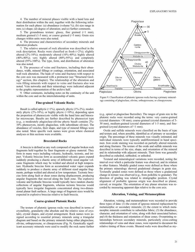
The texture of plutonic igneous rocks was described in terms of crystallinity, granularity (the absolute and the relative sizes of crys- tals), crystal shapes, and crystal arrangement. Rock names were as- signed according to essential primary minerals using a triangular diagram and based on the primary minerals being either plagioclase, olivine, orthopyroxene, or clinopyroxene (Fig. 9). Genetically signif- icant accessary minerals were used to modify the rock name further
Figure 9. Classification of plutonic igneous rocks having a primary mineral- ogy consisting of plagioclase, olivine, orthopyroxene, or clinopyroxene.
(e.g., spinel or plagioclase lherzolite). The ranges of grain size in the plutonic rocks were recorded using the terms: very coarse-grained (crystal diameters >30 mm), coarse-grained (crystal diameters of 5- 30 mm), medium-grained (crystal diameters of 1-5 mm), and fine- grained (crystal diameters of <1 mm).
Oxide and sulfide minerals were classified on the basis of type and texture and, where possible, identified as of primary or secondary origin. The percentage of these minerals was visually estimated, and individual minerals were typically undifferentiated in hand speci- men. Iron oxide staining was recorded on partially altered minerals and along fractures. The texture of the oxide and sulfide minerals was described in terms of the size, shape, and orientation of the mineral and its relationship with adjacent minerals. Their form was generally described as euhedral, subhedral, or anhedral.
Textural and mineralogical variations were recorded, noting the interval over which a particular feature was observed, and its relation to other features. Modally graded zones were defined as those where the primary mineralogy showed gradational changes in grain size. Texturally graded zones were defined as those where a gradational change in texture was observed (e.g., from poikilitic to granular). The direction of grading was related to stratigraphic position. Crystal alignment of probable igneous origin was described as planar, curved, or irregular. The orientation of any planar structure was re- corded by measuring apparent dips relative to the core axis.
Alteration, Veining, and Metamorphism
Alteration, veining, and metamorphism were recorded to provide three types of data: (1) the extent of igneous mineral replacement by metamorphic or secondary minerals; (2) the extent to which meta- morphic minerals contribute to subsolidus fabric; (3) the abundance, character, and orientation of veins, along with their associated haloes; and (4) the thickness and orientation of shear zones. Overprinting re- lationships between secondary minerals, particularly cross-cutting relationships of veins and shear zones, were reported to document the relative timing of these events. Sheared rocks were described as my-
21
SHIPBOARD SCIENTIFIC PARTY
lonites, cataclasites, or porphyroclastites, depending on the extent to which crushing, recrystallization, and fabric development had modi- fied the primary igneous rock. Identification of vein-filling material was frequently checked using XRD.
Individual vein types were identified by color and mineralogy. Data on abundance, width (mm), orientation, and texture and abun- dance of vein-filling minerals were recorded for each piece contain- ing one or more veins. In pieces having numerous veins, sequences, and patterns produced by intersecting veins and sequences of chang- ing mineralization in the veins were recorded and described.
Thin-section Descriptions
Thin sections of igneous rocks were examined to complement and refine hand-specimen observations. The same terminology was used for thin-section and visual-core descriptions. The percentages and textural descriptions of individual phases were recorded using a com- puterized database (HRTHIN). Thin-section descriptions are includ- ed in the "Cores" section (this volume) as separate tables for each core.
X-ray Diffraction Analyses
A Philips ADP 3520 X-ray diffractometer was used for the X-ray diffraction (XRD) analysis of mineral phases. Ni-filtered CuKα radi- ation generated at 40 kV and 35 mA was used. Peaks were scanned from a 2θ of 2° to 32°, with a step size of 0.02°, and a counting time of 2 sec/step.
Samples were ground to <200 µm mesh in a Spex 8000 Mixer Mill using tungsten carbide and steel. The powder then was pressed into aluminum sample holders or smeared onto glass plates for analysis. Diffractograms were interpreted with the help of a computerized search and match routine using the Joint Committee on Powder Dif- fraction Standards powder files.
X-ray Fluorescence Analysis
Before analysis, samples were crushed in a Spex 8510 shatterbox using a tungsten carbide barrel. Where recovery permitted, at least 20 cm3 of material was ground to ensure a representative sample. The
22
tungsten carbide barrel was used despite the considerable W contam- ination and minor Ta, Co, and Nb contamination, which makes the powder unsuitable for later instrumental neutron activation analysis (INAA).
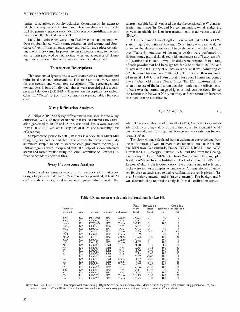
A fully automated wavelength-dispersive ARL8420 XRF (3 kW) system, equipped with an Rh-target X-ray tube, was used to deter- mine the abundances of major and trace elements in whole-rock sam- ples (Table 4). Analyses of the major oxides were performed on lithium borate glass disks doped with lanthanum as a "heavy absorb- er" (Norrish and Hutton, 1969). The disks were prepared from 500mg of rock powder that had been ignited for 2 hr at about 1030°C and mixed with 6.000 g dry flux (pre-weighed onshore) consisting of 80% lithium tetraborate and 20% La2O3. This mixture then was melt- ed in air at 1150°C in a Pt-Au crucible for about 10 min and poured into a Pt-Au mold using a Claisse fluxer. The 12:1 flux-to-sample ra- tio and the use of the lanthanum absorber made matrix effects insig- nificant over the normal range of igneous rock compositions. Hence, the relationship between X-ray intensity and concentration becomes linear and can be described by:
where Ci = concentration of element i (wt%); li = peak X-ray inten- sity of element i; mi = slope of calibration curve for element i (wt%/ counts/second); and bi = apparent background concentration for ele- ment i (wt%).
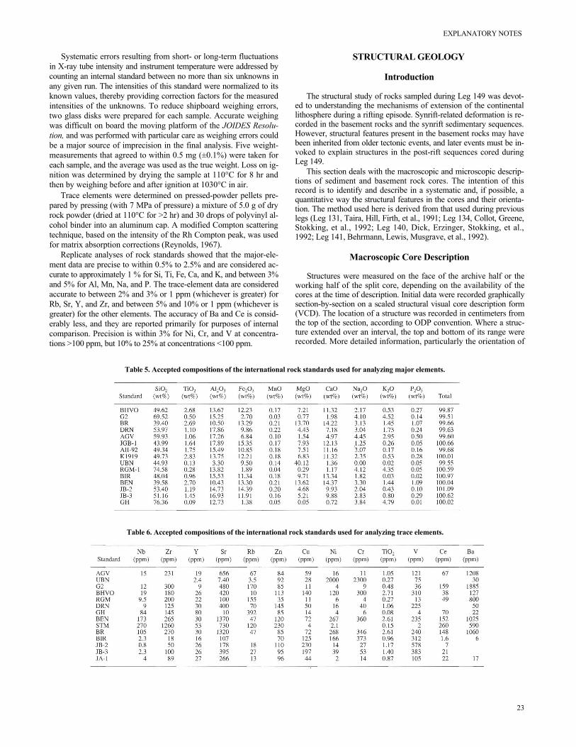
The slope mi was calculated from a calibration curve derived from the measurement of well-analyzed reference rocks, such as BEN, BR, and DRN from Geostandards, France; BHVO-1, RGM-1, and AGV- 1 from the U.S. Geological Survey; JGB-1 and JP-1 from the Geolog- ical Survey of Japan; AII-92-29-1 from Woods Hole Oceanographic Institution/Massachusetts Institute of Technology; and K1919 from Lamont-Doherty Earth Observatory. Two other standard reference rocks were run with samples as unknowns. A complete list of analy- ses for the standards used to derive calibration curves is given in Ta- bles 5 (major elements) and 6 (trace elements). The background bi was determined by regression analysis from the calibration curves.
Table 4. X-ray spectrograph analytical conditions for Leg 149.
Notes: Total Fe as Fe2O3*. FPC = Flow proportional counter using P10 gas; Scint = NaI scintillation counter. Major elements analyzed under vacuum using goniometer 2 at gener-
ator settings of 30 kV and 80 mA. Trace elements analyzed under vacuum using goniometer 2 at generator settings of 60 kV and 50mA.
EXPLANATORY NOTES
Systematic errors resulting from short- or long-term fluctuations in X-ray tube intensity and instrument temperature were addressed by counting an internal standard between no more than six unknowns in any given run. The intensities of this standard were normalized to its known values, thereby providing correction factors for the measured intensities of the unknowns. To reduce shipboard weighing errors, two glass disks were prepared for each sample. Accurate weighing was difficult on board the moving platform of the JOIDES Resolu- tion, and was performed with particular care as weighing errors could be a major source of imprecision in the final analysis. Five weight- measurements that agreed to within 0.5 mg (±0.1%) were taken for each sample, and the average was used as the true weight. Loss on ig- nition was determined by drying the sample at 110°C for 8 hr and then by weighing before and after ignition at 1030°C in air.
Trace elements were determined on pressed-powder pellets pre- pared by pressing (with 7 MPa of pressure) a mixture of 5.0 g of dry rock powder (dried at 110°C for >2 hr) and 30 drops of polyvinyl al- cohol binder into an aluminum cap. A modified Compton scattering technique, based on the intensity of the Rh Compton peak, was used for matrix absorption corrections (Reynolds, 1967).
Replicate analyses of rock standards showed that the major-ele- ment data are precise to within 0.5% to 2.5% and are considered ac- curate to approximately 1 % for Si, Ti, Fe, Ca, and K, and between 3% and 5% for Al, Mn, Na, and P. The trace-element data are considered accurate to between 2% and 3% or 1 ppm (whichever is greater) for Rb, Sr, Y, and Zr, and between 5% and 10% or 1 ppm (whichever is greater) for the other elements. The accuracy of Ba and Ce is consid- erably less, and they are reported primarily for purposes of internal comparison. Precision is within 3% for Ni, Cr, and V at concentra- tions >100 ppm, but 10% to 25% at concentrations <100 ppm.
STRUCTURAL GEOLOGY
Introduction
The structural study of rocks sampled during Leg 149 was devot- ed to understanding the mechanisms of extension of the continental lithosphere during a rifting episode. Synrift-related deformation is re- corded in the basement rocks and the synrift sedimentary sequences. However, structural features present in the basement rocks may have been inherited from older tectonic events, and later events must be in- voked to explain structures in the post-rift sequences cored during Leg 149.
This section deals with the macroscopic and microscopic descrip- tions of sediment and basement rock cores. The intention of this record is to identify and describe in a systematic and, if possible, a quantitative way the structural features in the cores and their orienta- tion. The method used here is derived from that used during previous legs (Leg 131, Taira, Hill, Firth, et al., 1991; Leg 134, Collot, Greene, Stokking, et al., 1992; Leg 140, Dick, Erzinger, Stokking, et al., 1992; Leg 141, Behrmann, Lewis, Musgrave, et al., 1992).
Macroscopic Core Description
Structures were measured on the face of the archive half or the working half of the split core, depending on the availability of the cores at the time of description. Initial data were recorded graphically section-by-section on a scaled structural visual core description form (VCD). The location of a structure was recorded in centimeters from the top of the section, according to ODP convention. Where a struc- ture extended over an interval, the top and bottom of its range were recorded. More detailed information, particularly the orientation of
Table 5. Accepted compositions of the international rock standards used for analyzing major elements.
Table 6. Accepted compositions of the international rock standards used for analyzing trace elements.
23

SHIPBOARD SCIENTIFIC PARTY
Figure 10. Terminology of structural identifiers used for structure observed in core during Leg 149.
structures, was recorded on a working core description form adapted from those devised during Leg 131 (Taira, Hill, Firth, et al, 1991) and on a computer spreadsheet. A numerical identifier was used to correlate individual structures between the three forms.
Description and Measurement of the Structures
The descriptive terminology for macroscopic features is listed in Figure 10. The terms may be modified by added descriptions and sketches. Natural structures often are difficult to distinguish from those caused by drilling and coring disturbance. Planar structures having polished surfaces and/or linear grooves were regarded as tec- tonic- rather than drilling-induced. In zones of brecciation, features were attributed to drilling disturbance if their tectonic origin was in doubt. The recommendations of Lundberg and Moore (1986, p. 42- 43) were followed for the sediments.
Several problems are inherent to this study. Commonly, only part of the core associated with any one core interval is actually recov- ered, leading to a sampling bias that for structural purposes is partic- ularly acute. Friable material from fault zones and low temperature shear zones in particular may be missing in cases of incomplete re- covery. When faulted or fractured rock from such zones is recovered, it is often highly disturbed and its original orientation altered.
Determining the orientation of observed structures (and intrusive dikes) is difficult. First, structures were oriented relative to core ref- erence coordinates (see below). This arbitrary reference frame will be related, if possible, to true north and true vertical using paleomagnet- ic, and Formation MicroScanner (FMS), data when available.
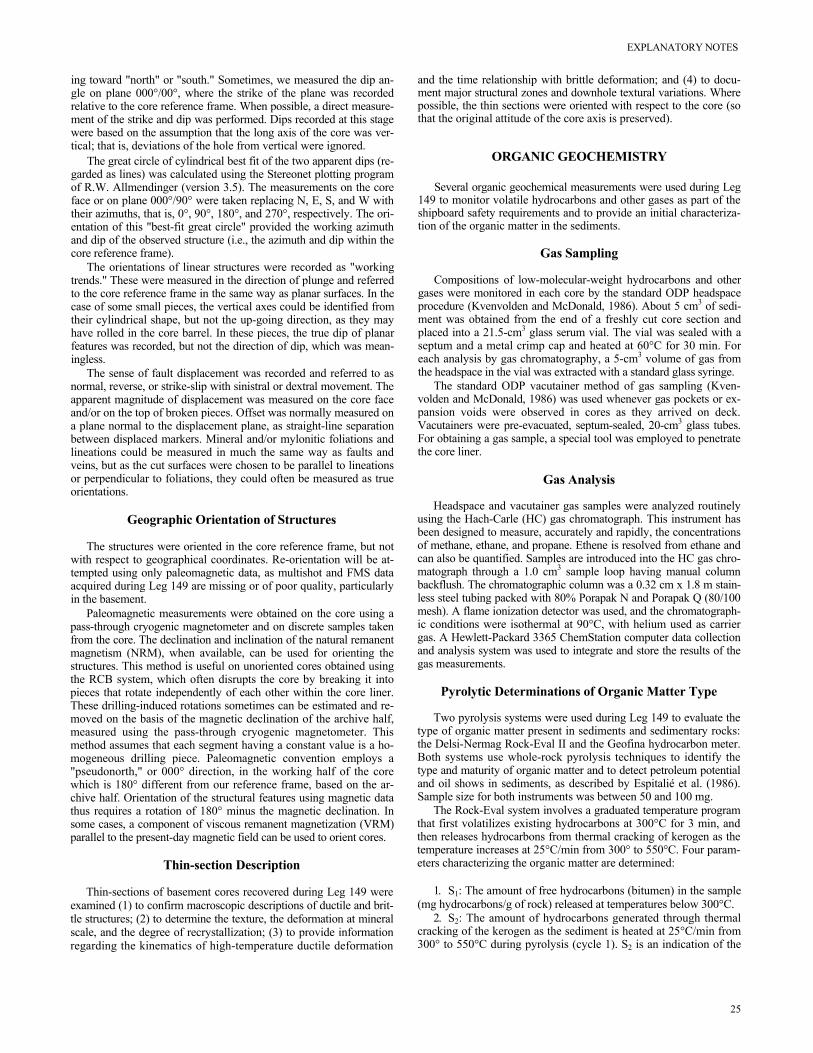
Our measurements of the orientations of structures observed in the cores were facilitated by a simple tool described in the "Explana- tory Notes" chapter of Leg 131 Initial Reports volume (Taira, Hill, Firth, et al., 1991). The dip of a structure exposed in the split core was recorded according to the convention illustrated in Figure 11. The plane normal to the axis of the borehole was referred to as the appar- ent horizontal plane. On this plane, a 360° net was used with a "pseudonorth" (000°) direction defined as the bottom of the semicir- cular archive-half core. Thus, the face of the split core (the core face) was the plane 090°/90° (strike, dip), and the plane at right angles to the core face and parallel to the core axis was the plane 000°/90°
24
(strike, dip). The apparent dip on the core face, either dipping toward the "east" or toward the "west" (looking at the face of the archive half of the core with its top looking upward), was measured. A second ap- parent dip was measured in one of the two planes, depending on expo- sure. Usually, we measured the dip in the plane 000°/90° at right angles to the core face, with the apparent dip direction in this plane be-
Figure 11. Conventions used for measuring azimuths and dips of structural features in the core and techniques used for measuring structural planes in three dimensions in the core reference frame. The core reference frame con- ventions for the working half and the archive half of the core can be seen in (A) and (B). The "E-W" (core reference frame) apparent dip of a feature was measured first and recorded as an apparent dip toward either 090° or 270° (in this case, the apparent dip is toward 090°). A second apparent dip was mea- sured by making a cut parallel to the core axis, but perpendicular to the core face in the working half of the core (A). The feature was identified on the new surface, and the apparent dip in the "N-S" (core reference frame) direc- tion was marked with a toothpick. The apparent dip was measured with a cli- nometer (C) and recorded as a value toward either 000° or 180°. In this diagram, the apparent dip is toward 180° (into the working half). True dip and strike of the surface in the core reference frame were calculated from the two apparent measurements.
EXPLANATORY NOTES
ing toward "north" or "south." Sometimes, we measured the dip an- gle on plane 000°/00°, where the strike of the plane was recorded relative to the core reference frame. When possible, a direct measure- ment of the strike and dip was performed. Dips recorded at this stage were based on the assumption that the long axis of the core was ver- tical; that is, deviations of the hole from vertical were ignored.
The great circle of cylindrical best fit of the two apparent dips (re- garded as lines) was calculated using the Stereonet plotting program of R.W. Allmendinger (version 3.5). The measurements on the core face or on plane 000°/90° were taken replacing N, E, S, and W with their azimuths, that is, 0°, 90°, 180°, and 270°, respectively. The ori- entation of this "best-fit great circle" provided the working azimuth and dip of the observed structure (i.e., the azimuth and dip within the core reference frame).
The orientations of linear structures were recorded as "working trends." These were measured in the direction of plunge and referred to the core reference frame in the same way as planar surfaces. In the case of some small pieces, the vertical axes could be identified from their cylindrical shape, but not the up-going direction, as they may have rolled in the core barrel. In these pieces, the true dip of planar features was recorded, but not the direction of dip, which was mean- ingless.
The sense of fault displacement was recorded and referred to as normal, reverse, or strike-slip with sinistral or dextral movement. The apparent magnitude of displacement was measured on the core face and/or on the top of broken pieces. Offset was normally measured on a plane normal to the displacement plane, as straight-line separation between displaced markers. Mineral and/or mylonitic foliations and lineations could be measured in much the same way as faults and veins, but as the cut surfaces were chosen to be parallel to lineations or perpendicular to foliations, they could often be measured as true orientations.
Geographic Orientation of Structures
The structures were oriented in the core reference frame, but not with respect to geographical coordinates. Re-orientation will be at- tempted using only paleomagnetic data, as multishot and FMS data acquired during Leg 149 are missing or of poor quality, particularly in the basement.
Paleomagnetic measurements were obtained on the core using a pass-through cryogenic magnetometer and on discrete samples taken from the core. The declination and inclination of the natural remanent magnetism (NRM), when available, can be used for orienting the structures. This method is useful on unoriented cores obtained using the RCB system, which often disrupts the core by breaking it into pieces that rotate independently of each other within the core liner. These drilling-induced rotations sometimes can be estimated and re- moved on the basis of the magnetic declination of the archive half, measured using the pass-through cryogenic magnetometer. This method assumes that each segment having a constant value is a ho- mogeneous drilling piece. Paleomagnetic convention employs a "pseudonorth," or 000° direction, in the working half of the core which is 180° different from our reference frame, based on the ar- chive half. Orientation of the structural features using magnetic data thus requires a rotation of 180° minus the magnetic declination. In some cases, a component of viscous remanent magnetization (VRM) parallel to the present-day magnetic field can be used to orient cores.
Thin-section Description
Thin-sections of basement cores recovered during Leg 149 were examined (1) to confirm macroscopic descriptions of ductile and brit- tle structures; (2) to determine the texture, the deformation at mineral scale, and the degree of recrystallization; (3) to provide information regarding the kinematics of high-temperature ductile deformation
and the time relationship with brittle deformation; and (4) to docu- ment major structural zones and downhole textural variations. Where possible, the thin sections were oriented with respect to the core (so that the original attitude of the core axis is preserved).
ORGANIC GEOCHEMISTRY
Several organic geochemical measurements were used during Leg 149 to monitor volatile hydrocarbons and other gases as part of the shipboard safety requirements and to provide an initial characteriza- tion of the organic matter in the sediments.
Gas Sampling
Compositions of low-molecular-weight hydrocarbons and other gases were monitored in each core by the standard ODP headspace procedure (Kvenvolden and McDonald, 1986). About 5 cm3 of sedi- ment was obtained from the end of a freshly cut core section and placed into a 21.5-cm3 glass serum vial. The vial was sealed with a septum and a metal crimp cap and heated at 60°C for 30 min. For each analysis by gas chromatography, a 5-cm3 volume of gas from the headspace in the vial was extracted with a standard glass syringe.
The standard ODP vacutainer method of gas sampling (Kven- volden and McDonald, 1986) was used whenever gas pockets or ex- pansion voids were observed in cores as they arrived on deck. Vacutainers were pre-evacuated, septum-sealed, 20-cm3 glass tubes. For obtaining a gas sample, a special tool was employed to penetrate the core liner.
Gas Analysis
Headspace and vacutainer gas samples were analyzed routinely using the Hach-Carle (HC) gas chromatograph. This instrument has been designed to measure, accurately and rapidly, the concentrations of methane, ethane, and propane. Ethene is resolved from ethane and can also be quantified. Samples are introduced into the HC gas chro- matograph through a 1.0 cm3 sample loop having manual column backflush. The chromatographic column was a 0.32 cm x 1.8 m stain- less steel tubing packed with 80% Porapak N and Porapak Q (80/100 mesh). A flame ionization detector was used, and the chromatograph- ic conditions were isothermal at 90°C, with helium used as carrier gas. A Hewlett-Packard 3365 ChemStation computer data collection and analysis system was used to integrate and store the results of the gas measurements.
Pyrolytic Determinations of Organic Matter Type
Two pyrolysis systems were used during Leg 149 to evaluate the type of organic matter present in sediments and sedimentary rocks: the Delsi-Nermag Rock-Eval II and the Geofina hydrocarbon meter. Both systems use whole-rock pyrolysis techniques to identify the type and maturity of organic matter and to detect petroleum potential and oil shows in sediments, as described by Espitalié et al. (1986). Sample size for both instruments was between 50 and 100 mg.
The Rock-Eval system involves a graduated temperature program that first volatilizes existing hydrocarbons at 300°C for 3 min, and then releases hydrocarbons from thermal cracking of kerogen as the temperature increases at 25°C/min from 300° to 550°C. Four param- eters characterizing the organic matter are determined:
1. S1: The amount of free hydrocarbons (bitumen) in the sample (mg hydrocarbons/g of rock) released at temperatures below 300°C.
2. S2: The amount of hydrocarbons generated through thermal cracking of the kerogen as the sediment is heated at 25°C/min from 300° to 550°C during pyrolysis (cycle 1). S2 is an indication of the
25
SHIPBOARD SCIENTIFIC PARTY
quantity of hydrocarbons that might have been produced in this rock, should deeper burial and greater thermal maturation have occurred.
3. S3: The quantity of CO2 (mg CO2/g of rock) produced from pyrolysis of the organic matter at temperatures between 300° and 390°C.
4. Tmax: Maturity of the organic material assessed by the tempera- ture at which the maximum release of hydrocarbons from cracking of kerogen occurs during pyrolysis (top of the S2 peak).
The Rock-Eval II instrument is equipped with a module that uses an algorithm and the S1, S2, and S3 peak values to estimate the total amount of organic carbon (TOC) in samples.
Organic matter can be characterized from Rock-Eval data using the hydrogen index [(100 × S2)OC], the oxygen index [(100 × S3)OC], and the S2/S3 ratio. The first two parameters normally are referred to as HI and OI, respectively. Interpretations of Rock-Eval pyrolysis are considered to be unreliable for samples having less than 0.5% TOC (Katz, 1983; Peters, 1986), although a correction procedure has been described for estimating matrix effects and for obtaining reliable val- ues from samples having lower amounts of TOC (Espitalié, 1980).
The Geofina hydrocarbon meter (GHM) employs a Varian 3400 series gas chromatograph that has been modified to include a pro- grammable pyrolysis injector. The system has three flame ionization detectors and two capillary columns (25 m, GC2 fused silica). Like the Rock-Eval II, this tool determines S1, the free hydrocarbons that are released up to 300°C, and S2, the pyrolysis products that are gen- erated from the sample kerogen. Tmax of the S2 peak also is deter- mined. The effluent from the furnace is split 20:1 so that the hydrocarbon distributions making up S1 and S2 can be examined in detail by capillary gas chromatography. Rock-Eval and GHM param- eters can be used to calculate the production index (PI) = S2/(S1 + S2), and petroleum potential or pyrolyzed carbon index (PC) = 0.083(S1 + S2).
Carbonate Carbon
The carbonate carbon content of samples was determined using a Coulometrics 5011 inorganic carbon analyzer (Engleman et al., 1985). A sample of about 20 mg of freeze-dried and ground material was reacted with 2N HCl. The liberated CO2 was titrated in an etha- nolamine solution containing a color indicator, and the change in col- or was measured by a photodetector cell. Carbonate carbon contents are expressed as weight percent CaCO3, assuming all the carbonate was present as pure calcite.
Organic Carbon
The total organic carbon content (TOC) of sediment samples was determined either by the Rock-Eval TOC module or by the difference between carbonate carbon and the total carbon value determined by the Carlo Erba Model NA 1500 NCS analyzer. In the NCS analyzer, freeze-dried and ground samples were combusted at 1000°C in an ox- ygen stream. Nitrogen oxides were reduced to N2, and the mixture of CO2, SO2, and N2 was separated by gas chromatography and quanti- fied with a thermal conductivity detector.
INORGANIC GEOCHEMISTRY
The shipboard analytical program for inorganic geochemistry fo- cused solely on the chemical characterization of interstitial waters ex- tracted from 5- to 15-cm-long whole-round sediment samples and/or taken with the in-situ sampler (the WSTP tool). During Leg 149, in- terstitial waters for shore-based analyses of trace elements were ob- tained by squeezing sediments with a plastic-lined squeezer designed
26
by Hans Brumsack. Interstitial water samples for shipboard analysis and for ODP archives were collected either with the Brumsack squeezer or with a titanium Manheim squeezer.
The whole-round sections were cut from the core immediately af- ter it arrived on deck and were placed in a nitrogen-filled glove bag to prevent oxidation. While in the nitrogen bag, the sediment was re- moved from the core liner, scraped with a plastic spatula, and loaded into the plastic-lined squeezer. Highly consolidated sediments were broken into small pieces and a portion transferred to the titanium squeezer. The sediment was squeezed at pressures up to 18,000 psi (124 MPa) in the Brumsack squeezer and up to 40,000 psi (276 MPa) in the titanium squeezer. The effluent from the Brumsack squeezer was ejected through a pre-cleaned 0.45-µm Millipore polycarbonate membrane placed inside the squeezer. In addition, the effluent was filtered through in-line pre-cleaned 0.22-µm acrodisk filters before collection in pre-cleaned syringes. The effluent from the titanium squeezer was filtered through an uncleaned 0.22-µm acrodisk filter. Effluent from each sediment sample was collected for shipboard analyses, for ODP archives, and for shore-based analyses of trace el- ements. The trace-element samples were transferred from the pre- cleaned plastic syringes to pre-cleaned plastic vials acidified with Ul- trex HCl and stored. Samples for shipboard analyses were refrigerat- ed, and archive samples were sealed in glass ampules.
Analytical Methods
Alkalinity and pH were determined in duplicate immediately fol- lowing sample collection using the Metrohm autotitrator with a Brinkman combination pH electrode. The electrode was calibrated prior to analysis and periodically checked for drift. Salinity was esti- mated using a Goldberg optical hand refractometer to measure the to- tal dissolved solids. The concentrations of the sulfate and chloride anions and the calcium, magnesium, sodium, and potassium cations were determined in duplicate using a Dionex-DX100 ion chromato- graph. All samples were run at 1:200 dilution. Standards were run at the start and end of each run to test for drift in the response of the con- ductivity detector. Precision of separate dilutions was better than 2%. Concentrations of ammonium, silica, and phosphate were determined by the spectrophotometric techniques described in Gieskes and Peretsman (1986). Concentrations of iron, manganese, and strontium were analyzed by atomic absorption spectrophotometry (AAS).
PHYSICAL PROPERTIES Introduction
Nondestructive measurements were made on whole sections of core using the multisensor track (MST). This incorporated the Gam- ma Ray Attenuation Porosity Evaluator (GRAPE), P-wave logger (PWL), and magnetic susceptibility sensors. Thermal conductivities were measured for sediments and basement rocks using the needle probe method. When the sediment was soft enough, compressional wave velocities, undrained shear strengths, and electrical resistivities were measured on the working half of the core. In addition, discrete samples were taken throughout the cores for determining index prop- erties and compressional wave velocities.
Nondestructive Measurements Multisensor Track
The MST incorporates the GRAPE, PWL, and magnetic suscep- tibility sensors. A natural gamma-ray sensor was added to the MST at the beginning of Leg 149, which was used only on selected cores for testing the instrument. Individual unsplit core sections were
EXPLANATORY NOTES
placed horizontally on the MST, which moves the section past the four sensors.
The GRAPE measures bulk density at 1 cm intervals (minimum) by comparing the attenuation of gamma rays through the cores with attenuation through aluminum and water standards (Boyce, 1976). The GRAPE data are most reliable in APC and fullsized XCB and RCB cores and offer the potential of direct correlation with downhole bulk density logs. For the preliminary on-board processing, only ev- ery 20th measurement was used. Corrections were made for varia- tions in core diameter, pore water composition, and mineralogy, following Evans and Cotterell (1970), Boyce (1976), and Lloyd and Moran (unpubl. data). For very disturbed cores, the GRAPE acquisi- tion was turned off.
The PWL transmits a 500-kHz compressional-wave pulse through the core at a repetition rate of 1 kHz. The transmitting and receiving transducers are aligned perpendicular to the long axis of the core. A pair of displacement transducers monitors the separation between the compressional wave transducers; variations in the outside diameter of the liner therefore do not degrade the accuracy of the velocities. Measurements are taken at 3-cm intervals. Generally, only the APC and fullsized XCB and RCB cores were measured. The quality of the data was assessed by examining the arrival time and amplitude of the received pulse. Data having anomalously large traveltimes or low amplitudes were discarded.
Magnetic susceptibility was measured on all sections at intervals of 3 to 5 cm using the 1.0 range on the Bartington Instruments mag- netic susceptibility meter (model MS2) with an 8-cm-diameter loop. The magnetic susceptibility provides another measure to assist cross- hole correlations and can help to detect fine variations in magnetic in- tensity associated with magnetic reversals. The quality of these re- sults degrades in XCB and RCB sections where the core liner is not completely filled and/or the core is disturbed. However, the general downhole trends may still be used for stratigraphic correlation.
Thermal Conductivity
Whole-round core sections were allowed to adjust to room tem- perature for at least 4 hr before measuring thermal conductivities. The needle probe method was used in full-space configuration for soft sediments (Von Herzen and Maxwell, 1959), and in half-space mode for lithified sediment and hard rock samples (Vacquier, 1985). Thermal conductivities were typically measured in alternate sections. During transit to the first site and at irregular intervals during the cruise, the needle probes were calibrated vs. known standards (red rubber, black rubber, and macor), providing for five measurements in each standard per needle. A least-squares linear regression of known thermal conductivity and measured conductivity was performed for each needle to provide the corrections used for data reduction. Data are reported in units of (W/m·K), with an uncertainty of 5% to 10%, estimated from the regression line.
Soft Sediment "Full-Space" Measurements
Needle probes, containing a heater wire and a calibrated ther- mistor, were inserted into the sediment through small holes drilled into the core liners before the sections were split. The probes were positioned where the sample appeared to show uniform properties. Data were acquired using a Thermcon-85 unit interfaced to an IBM- PC compatible microcomputer. This system allowed up to five probes to be connected and operated simultaneously. For quality con- trol, one probe was used with a standard of known conductivity dur- ing each run.
At the beginning of each measurement, temperatures in the sam- ples were monitored without applying current to the heating element to verify that temperature drift was less than 0.04°C/min. The heater then was turned on and the temperature rise in the probes was record-
ed. After heating for about 60 s, the needle probe response behaves nearly as a line source with constant heat generation per unit length. Temperatures recorded between 60 and 240 s were fit to the follow- ing equation using the least-squares method (Von Herzen and Max- well, 1959):
where A represents the rate of temperature change, and Te is the equilibrium temperature. L(t) therefore corrects for the background temperature drift, systematic instrumental errors, probe response, and sample geometry. The best fit to the data determines the unknown terms k and A.
Lithified Sediment and Hard Rock "Half-Space" Measurements
Half-space measurements were performed on selected lithified sediments and crystalline rock samples after the cores were split and the faces of the split cores were polished. The needle probe rested be- tween the polished surface and a grooved epoxy block having rela- tively low conductivity (Sass et al., 1984; Vacquier, 1985). Half- space measurements were conducted in a water bath to keep the sam- ples saturated, to improve the thermal contact between the needle and the sample, and to reduce thermal drift. EG&G thermal joint com- pound was used to improve the thermal contact. Data collection and reduction procedures for half-space tests are similar to those for full- space tests, except for a multiplicative constant in Equation 3 that ac- counts for the different experimental geometry.
Discrete Measurements
Index Properties
Index properties, including bulk density, grain density, water con- tent, and porosity, were calculated from measurements of wet and dry sample masses and wet volumes. On samples of approximately 10 cm3 dry sample volumes, which can be determined indirectly from the raw measurements listed above, also were measured directly, al- lowing one to check the calculations. In addition, bulk density was measured on unsplit cores using the GRAPE, as discussed above.
Sample mass was determined to a precision of ±0.01 g using a Scitech electronic balance. The sample mass was counterbalanced by a known mass such that the mass differentials generally were less than 1 g. Sample volumes were determined using a Quantachrome Penta-Pycnometer, a helium-displacement pycnometer with a nomi- nal precision of ±0.02 cm3, but a lower apparent experimental preci- sion. Sample volumes were measured at least twice, and the mean of the readings was taken to be the volume. A reference volume was run with each group of samples, and rotated among the cells to check for systematic error. This exercise demonstrated that the measured vol- umes had a precision of about 0.03 cm3. The pycnometer volumes were re-calibrated frequently during use for both small and large sample holders. The sample beakers used for discrete determinations of index properties were calibrated carefully prior to the cruise.
where k is the apparent thermal conductivity (W/m·K), T is tempera-ture (°C), t is time (s), and q is the heat input per unit length of wireper unit time. The term L(t) corrects for a linear change in tempera-ture with time, described by the following equation:
27
SHIPBOARD SCIENTIFIC PARTY
Water Content
There are two definitions for pore-water content: (1) Wd, pore-wa- ter mass divided by the mass of solids Ms, and (2) Ww, pore-water mass divided by total mass Mt. When determining water content, the methods of the American Society for Testing and Materials were fol- lowed (ASTM, designation [D] 2216; ASTM, 1989). The total (Mt) and dry (Md) masses were measured using the electronic balance. The difference (Mt-Md), after correction for salt by assuming a pore-water salinity (r) of 0.035, following the discussion by Boyce (1976), was taken as the pore-fluid mass. The equations for the two water-content calculations are as follows:
Bulk Density and Grain Density
Bulk density (ρ) is the density of the total sample including the pore fluid (i.e., ρ = Mt/Vt, where Vt is the total sample volume [cm3] measured with the helium pycnometer).
Grain Density
Grain density, ρg is determined from the dry mass (Scitec balance)and dry volume (pycnometer) measurements. In this case, both massand volume must be corrected for salinity, leading to the followingequation: is the density of salt (2.257 g/cm3).
where Vd is the dry volume (cm3) and ρs is the density of salt (2.257 g/cm3). Ms = r · Mw is the mass of salt in the pore fluid, Mw is the mass of the seawater:
To check these determinations, and to assess the quality of the volumes derived from the helium pycnometer, grain density was es- timated occasionally using dry volume measurements in powdered samples.
Porosity
Porosity (η), the ratio of the fully saturated pore-water volume to the total volume, can be determined several ways using the quantities derived above. The following relationship using calculated grain den- sity, ρg, and bulk density ρ was employed:
where ρg is grain density, ρ is bulk density and ρw is seawater den- sity. To check for internal consistency, porosities also were calcu- lated using the relationship:
28
where ρ is bulk density and Wd is water content (dry mass).
Velocity Measurements
Discrete compressional-wave (P-wave) velocity measurements were obtained using two different systems, depending on the degree of lithification of the material. A Digital Sound Velocimeter (DSV) is a digital data acquisition system developed to measure and record compressional wave velocities and attenuation in soft sediments. The velocity calculation is based on the traveltime of an acoustic impulse between two piezoelectric transducers that are inserted directly into the split core. The transducers emit a 2-µs pulse having a repetition rate of 60 Hz. Gains from 0 to 42 dB can be applied to the received signal. The transmitted and received signals are displayed by a Nico- let 320 digital oscilloscope and transferred to a microcomputer for processing. The DSV software sums the waveforms from 3 to 10 suc- cessive digital records and displays the resulting waveform on the os- cilloscope. Traveltime is estimated by visual identification of the first break on the stacked waveform and is corrected for the total delay caused by the transducers and other velocimeter hardware. Velocity is determined from the corrected traveltime and the measured dis- tance (by caliper) between the transducers. The traveltime correction was determined by measuring the velocity of a distilled water sample and comparing the result to the standard water velocity (Wilson, 1960).
The Hamilton Frame Velocimeter (Hamilton, 1971) was used to measure compressional-wave velocities for well-indurated sedi- ments, lithified sediments, and crystalline rocks. Velocity was deter- mined using an impulsive signal having a frequency of 500 kHz. Cubes were trimmed from the sediment samples using a knife, with faces oriented parallel to the axis and split surface of the core. Veloc- ity was measured in three mutually perpendicular directions, V (along the core axis), Hx (perpendicular to core axis and parallel to core face), and Hy (perpendicular to core face). The magnitude of acoustic anisotropy was estimated according to the relationship:
where Vmax and Vmin are the maximum and minimum velocities (among V, Hx, and Hy). In crystalline rocks minicore samples (2.54- cm diameter) were drilled perpendicular to the axis and face of the core. The ends of the minicores were trimmed parallel with a rock saw, and velocity (Hy) was measured along the axis of the minicore. Whenever possible, velocity measurements were made adjacent to paleomagnetic measurements, to allow the possibility of orientating the samples to geographic coordinates.
The dimensions of samples measured in the Hamilton Frame were determined with a digital linear caliper. Traveltime was estimated by visual identification of the first break of the stacked waveform, as de- scribed for the DSV measurements. Traveltime was corrected for the total delays caused by the transducers and velocimeter hardware. This was estimated by a linear regression of traveltime vs. distance for a series of aluminum and lucite standards. Velocities were calcu- lated from the corrected traveltimes and measured sample dimen- sions. Velocity data are reported here in raw form; however, corrections to in-situ temperature and pressure also can be made us- ing the relationships in Wyllie et al. (1956).
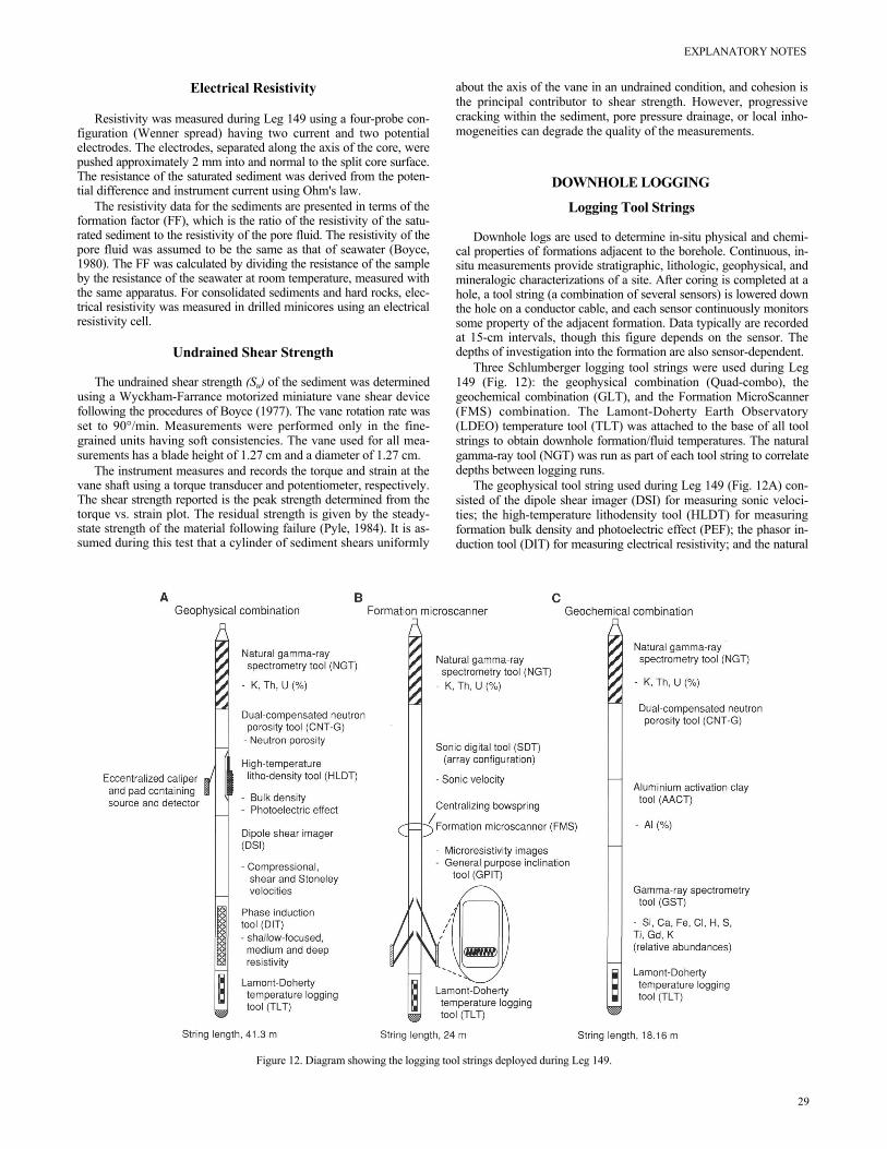
EXPLANATORY NOTES
Electrical Resistivity
Resistivity was measured during Leg 149 using a four-probe con- figuration (Wenner spread) having two current and two potential electrodes. The electrodes, separated along the axis of the core, were pushed approximately 2 mm into and normal to the split core surface. The resistance of the saturated sediment was derived from the poten- tial difference and instrument current using Ohm's law.
The resistivity data for the sediments are presented in terms of the formation factor (FF), which is the ratio of the resistivity of the satu- rated sediment to the resistivity of the pore fluid. The resistivity of the pore fluid was assumed to be the same as that of seawater (Boyce, 1980). The FF was calculated by dividing the resistance of the sample by the resistance of the seawater at room temperature, measured with the same apparatus. For consolidated sediments and hard rocks, elec- trical resistivity was measured in drilled minicores using an electrical resistivity cell.
Undrained Shear Strength
The undrained shear strength (Su) of the sediment was determined using a Wyckham-Farrance motorized miniature vane shear device following the procedures of Boyce (1977). The vane rotation rate was set to 90°/min. Measurements were performed only in the fine- grained units having soft consistencies. The vane used for all mea- surements has a blade height of 1.27 cm and a diameter of 1.27 cm.
The instrument measures and records the torque and strain at the vane shaft using a torque transducer and potentiometer, respectively. The shear strength reported is the peak strength determined from the torque vs. strain plot. The residual strength is given by the steady- state strength of the material following failure (Pyle, 1984). It is as- sumed during this test that a cylinder of sediment shears uniformly
about the axis of the vane in an undrained condition, and cohesion is the principal contributor to shear strength. However, progressive cracking within the sediment, pore pressure drainage, or local inho- mogeneities can degrade the quality of the measurements.
DOWNHOLE LOGGING
Logging Tool Strings
Downhole logs are used to determine in-situ physical and chemi- cal properties of formations adjacent to the borehole. Continuous, in- situ measurements provide stratigraphic, lithologic, geophysical, and mineralogic characterizations of a site. After coring is completed at a hole, a tool string (a combination of several sensors) is lowered down the hole on a conductor cable, and each sensor continuously monitors some property of the adjacent formation. Data typically are recorded at 15-cm intervals, though this figure depends on the sensor. The depths of investigation into the formation are also sensor-dependent.
Three Schlumberger logging tool strings were used during Leg 149 (Fig. 12): the geophysical combination (Quad-combo), the geochemical combination (GLT), and the Formation MicroScanner (FMS) combination. The Lamont-Doherty Earth Observatory (LDEO) temperature tool (TLT) was attached to the base of all tool strings to obtain downhole formation/fluid temperatures. The natural gamma-ray tool (NGT) was run as part of each tool string to correlate depths between logging runs.
The geophysical tool string used during Leg 149 (Fig. 12A) con- sisted of the dipole shear imager (DSI) for measuring sonic veloci- ties; the high-temperature lithodensity tool (HLDT) for measuring formation bulk density and photoelectric effect (PEF); the phasor in- duction tool (DIT) for measuring electrical resistivity; and the natural
Figure 12. Diagram showing the logging tool strings deployed during Leg 149.
29
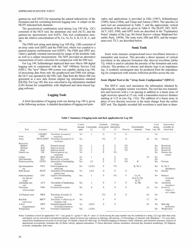
SHIPBOARD SCIENTIFIC PARTY
gamma-ray tool (NGT) for measuring the natural radioactivity of the formation and for correlating between logging runs. A caliper on the HLDT indicated hole diameter.
The geochemical combination used during Leg 149 (Fig. 12C) consisted of the NGT tool, the aluminum clay tool (ACT), and the gamma-ray spectrometry tool (GST). This tool combination mea- sures the relative concentrations of Si, Ca, Al, Fe, S, H, Cl, K, U, and Th.
The FMS tool string used during Leg 149 (Fig. 12B) consisted of an array sonic tool (SDT) and the FMS tool, which was coupled to a general purpose inclinometer tool (GPIT). The FMS and GPIT pro- vided a spatially oriented microresistivity image of the borehole wall, as well as a caliper measurement. The SDT provided an alternative measurement of sonic velocities for comparison with the DSI tool.
For Leg 149, Schlumberger deployed their new Maxis 500 digital logging unit in conjunction with the "old" Offshore Service Unit (OSU). The "new" Maxis 500 system was capable, during Leg 149, of processing data from only the geophysical and FMS tool strings; the GLT was operated by the OSU unit. Data from the Maxis 500 was generated in a new data format (digital log information standard [DLIS]). For Leg 149, this was converted to log information standard (LIS) format for compatibility with shipboard and shore-based log- ging software.
Logging Tools
A brief description of logging tools run during Leg 149 is given in the following sections. A detailed description of logging tool prin-
30
ciples and applications is provided in Ellis (1987), Schlumberger (1989), Serra (1984), and Timur and Toksöz (1985). The specifics of each tool are summarized in Table 7, and the approximate vertical resolutions of the tools are given in Table 8. The HLDT, DIT, NGT, ACT, GST, FMS, and GPIT tools are described in the "Explanatory Notes" chapter of the Leg 144 Initial Reports volume Shipboard Sci- entific Party, 1993b). The sonic tools, DSI and SDT, and the temper- ature tool, TLT, are described below.
Sonic Tools
Sonic tools measure compressional-wave traveltimes between a transmitter and receiver. This provides a direct measure of vertical traveltime in the adjacent formation (the interval traveltime [delta T]), which is used to calculate the porosity of the formation and sonic velocity. The product of velocity and density logs is an impedance log. A synthetic seismogram may be produced from the impedance log for comparison with seismic reflection profiles across the site.
Sonic Digital Tool or the "Array Sonic Configuration" (SDT-C)
The SDT-C sonic tool maximizes the information obtained by digitizing the complete seismic waveform. The tool has two transmit- ters and receivers with a 1-m spacing in addition to a linear array of eight receivers spaced at 15 cm, with a transmitter-receiver distance starting at 3.33 m (see Fig. 13A). The addition of a linear array in place of two discrete receivers is the main change from the earlier SDT tool. The digitally recorded full waveform is used later to deter-
Table 7. Summary of logging tools and their application for Leg 149.
Notes: Usefulness of tool for application: VG = very good; G = good; F= fair; P = poor. (1) Tools having the same number may be combined in a string. (2) Logs other than sonic
and density can be converted to pseudosonic/density, based on known log responses to lithology and porosity. (3) Percentages of minerals with abundance > 3% were deter- mined from simultaneous inversion of several logs. (4) Quality control for other logs. (5) Detailed mapping of fractures, faults, foliations, and formation structures; analysis of depositional environments; formation dip. (6) Shear velocity, apparent attenuation. (7) Stress directions, fracture orientation, structural dip, formation morphology. (8) Magnetic reversals, stratigraphy, fault zones.
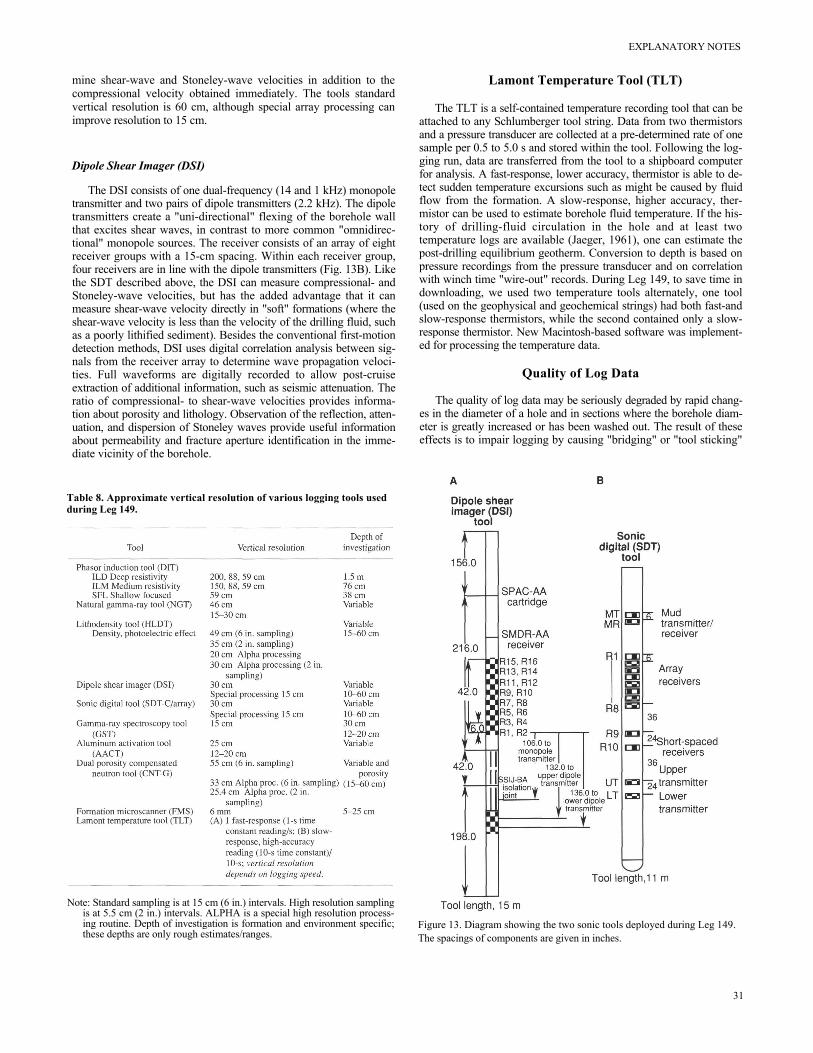
EXPLANATORY NOTES
mine shear-wave and Stoneley-wave velocities in addition to the compressional velocity obtained immediately. The tools standard vertical resolution is 60 cm, although special array processing can improve resolution to 15 cm.
Dipole Shear Imager (DSI)
The DSI consists of one dual-frequency (14 and 1 kHz) monopole transmitter and two pairs of dipole transmitters (2.2 kHz). The dipole transmitters create a "uni-directional" flexing of the borehole wall that excites shear waves, in contrast to more common "omnidirec- tional" monopole sources. The receiver consists of an array of eight receiver groups with a 15-cm spacing. Within each receiver group, four receivers are in line with the dipole transmitters (Fig. 13B). Like the SDT described above, the DSI can measure compressional- and Stoneley-wave velocities, but has the added advantage that it can measure shear-wave velocity directly in "soft" formations (where the shear-wave velocity is less than the velocity of the drilling fluid, such as a poorly lithified sediment). Besides the conventional first-motion detection methods, DSI uses digital correlation analysis between sig- nals from the receiver array to determine wave propagation veloci- ties. Full waveforms are digitally recorded to allow post-cruise extraction of additional information, such as seismic attenuation. The ratio of compressional- to shear-wave velocities provides informa- tion about porosity and lithology. Observation of the reflection, atten- uation, and dispersion of Stoneley waves provide useful information about permeability and fracture aperture identification in the imme- diate vicinity of the borehole.
Table 8. Approximate vertical resolution of various logging tools used during Leg 149.
Note: Standard sampling is at 15 cm (6 in.) intervals. High resolution sampling
is at 5.5 cm (2 in.) intervals. ALPHA is a special high resolution process- ing routine. Depth of investigation is formation and environment specific; these depths are only rough estimates/ranges.
Lamont Temperature Tool (TLT)
The TLT is a self-contained temperature recording tool that can be attached to any Schlumberger tool string. Data from two thermistors and a pressure transducer are collected at a pre-determined rate of one sample per 0.5 to 5.0 s and stored within the tool. Following the log- ging run, data are transferred from the tool to a shipboard computer for analysis. A fast-response, lower accuracy, thermistor is able to de- tect sudden temperature excursions such as might be caused by fluid flow from the formation. A slow-response, higher accuracy, ther- mistor can be used to estimate borehole fluid temperature. If the his- tory of drilling-fluid circulation in the hole and at least two temperature logs are available (Jaeger, 1961), one can estimate the post-drilling equilibrium geotherm. Conversion to depth is based on pressure recordings from the pressure transducer and on correlation with winch time "wire-out" records. During Leg 149, to save time in downloading, we used two temperature tools alternately, one tool (used on the geophysical and geochemical strings) had both fast-and slow-response thermistors, while the second contained only a slow- response thermistor. New Macintosh-based software was implement- ed for processing the temperature data.
Quality of Log Data
The quality of log data may be seriously degraded by rapid chang- es in the diameter of a hole and in sections where the borehole diam- eter is greatly increased or has been washed out. The result of these effects is to impair logging by causing "bridging" or "tool sticking"
Figure 13. Diagram showing the two sonic tools deployed during Leg 149. The spacings of components are given in inches.
31
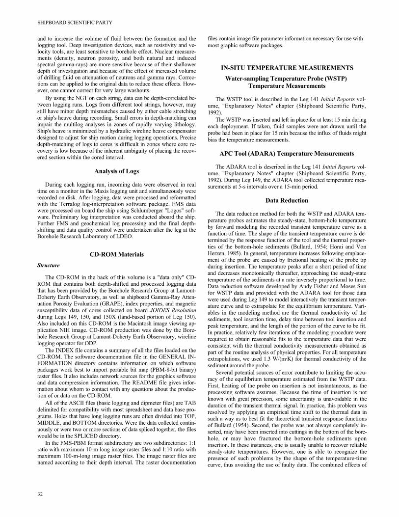
SHIPBOARD SCIENTIFIC PARTY
and to increase the volume of fluid between the formation and the logging tool. Deep investigation devices, such as resistivity and ve- locity tools, are least sensitive to borehole effect. Nuclear measure- ments (density, neutron porosity, and both natural and induced spectral gamma-rays) are more sensitive because of their shallower depth of investigation and because of the effect of increased volume of drilling fluid on attenuation of neutrons and gamma rays. Correc- tions can be applied to the original data to reduce these effects. How- ever, one cannot correct for very large washouts.
By using the NGT on each string, data can be depth-correlated be- tween logging runs. Logs from different tool strings, however, may still have minor depth mismatches caused by either cable stretching or ship's heave during recording. Small errors in depth-matching can impair the multilog analyses in zones of rapidly varying lithology. Ship's heave is minimized by a hydraulic wireline heave compensator designed to adjust for ship motion during logging operations. Precise depth-matching of logs to cores is difficult in zones where core re- covery is low because of the inherent ambiguity of placing the recov- ered section within the cored interval.
Analysis of Logs
During each logging run, incoming data were observed in real time on a monitor in the Maxis logging unit and simultaneously were recorded on disk. After logging, data were processed and reformatted with the Terralog log-interpretation software package. FMS data were processed on board the ship using Schlumberger "Logos" soft- ware. Preliminary log interpretation was conducted aboard the ship. Further FMS and geochemical log processing and the final depth- shifting and data quality control were undertaken after the leg at the Borehole Research Laboratory of LDEO.
CD-ROM Materials Structure
The CD-ROM in the back of this volume is a "data only" CD- ROM that contains both depth-shifted and processed logging data that has been provided by the Borehole Research Group at Lamont- Doherty Earth Observatory, as well as shipboard Gamma-Ray Atten- uation Porosity Evaluation (GRAPE), index properties, and magnetic susceptibility data of cores collected on board JOIDES Resolution during Legs 149, 150, and 150X (land-based portion of Leg 150). Also included on this CD-ROM is the Macintosh image viewing ap- plication NIH image. CD-ROM production was done by the Bore- hole Research Group at Lamont-Doherty Earth Observatory, wireline logging operator for ODP.
The INDEX file contains a summary of all the files loaded on the CD-ROM. The software documentation file in the GENERAL IN- FORMATION directory contains information on which software packages work best to import portable bit map (PBM-8-bit binary) raster files. It also includes network sources for the graphics software and data compression information. The README file gives infor- mation about whom to contact with any questions about the produc- tion of or data on the CD-ROM.
All of the ASCII files (basic logging and dipmeter files) are TAB delimited for compatibility with most spreadsheet and data base pro- grams. Holes that have long logging runs are often divided into TOP, MIDDLE, and BOTTOM directories. Were the data collected contin- uously or were two or more sections of data spliced together, the files would be in the SPLICED directory.
In the FMS-PBM format subdirectory are two subdirectories: 1:1 ratio with maximum 10-m-long image raster files and 1:10 ratio with maximum 100-m-long image raster files. The image raster files are named according to their depth interval. The raster documentation
32
files contain image file parameter information necessary for use with most graphic software packages.
IN-SITU TEMPERATURE MEASUREMENTS
Water-sampling Temperature Probe (WSTP) Temperature Measurements
The WSTP tool is described in the Leg 141 Initial Reports vol- ume, "Explanatory Notes" chapter (Shipboard Scientific Party, 1992).
The WSTP was inserted and left in place for at least 15 min during each deployment. If taken, fluid samples were not drawn until the probe had been in place for 15 min because the influx of fluids might bias the temperature measurements.
APC Tool (ADARA) Temperature Measurements
The ADARA tool is described in the Leg 141 Initial Reports vol- ume, "Explanatory Notes" chapter (Shipboard Scientific Party, 1992). During Leg 149, the ADARA tool collected temperature mea- surements at 5-s intervals over a 15-min period.
Data Reduction
The data reduction method for both the WSTP and ADARA tem- perature probes estimates the steady-state, bottom-hole temperature by forward modeling the recorded transient temperature curve as a function of time. The shape of the transient temperature curve is de- termined by the response function of the tool and the thermal proper- ties of the bottom-hole sediments (Bullard, 1954; Horai and Von Herzen, 1985). In general, temperature increases following emplace- ment of the probe are caused by frictional heating of the probe tip during insertion. The temperature peaks after a short period of time and decreases monotonically thereafter, approaching the steady-state temperature of the sediments at a rate inversely proportional to time. Data reduction software developed by Andy Fisher and Moses Sun for WSTP data and provided with the ADARA tool for those data were used during Leg 149 to model interactively the transient temper- ature curve and to extrapolate for the equilibrium temperature. Vari- ables in the modeling method are the thermal conductivity of the sediments, tool insertion time, delay time between tool insertion and peak temperature, and the length of the portion of the curve to be fit. In practice, relatively few iterations of the modeling procedure were required to obtain reasonable fits to the temperature data that were consistent with the thermal conductivity measurements obtained as part of the routine analysis of physical properties. For all temperature extrapolations, we used 1.3 W/(m·K) for thermal conductivity of the sediment around the probe.
Several potential sources of error contribute to limiting the accu- racy of the equilibrium temperature estimated from the WSTP data. First, heating of the probe on insertion is not instantaneous, as the processing software assumes. Because the time of insertion is not known with great precision, some uncertainty is unavoidable in the duration of the transient thermal signal. In practice, this problem was resolved by applying an empirical time shift to the thermal data in such a way as to best fit the theoretical transient response functions of Bullard (1954). Second, the probe was not always completely in- serted, may have been inserted into cuttings in the bottom of the bore- hole, or may have fractured the bottom-hole sediments upon insertion. In these instances, one is usually unable to recover reliable steady-state temperatures. However, one is able to recognize the presence of such problems by the shape of the temperature-time curve, thus avoiding the use of faulty data. The combined effects of
EXPLANATORY NOTES
these uncertainties can lead to an estimated accuracy of ± 0.1 °C in the unreduced temperature measurements.
Temperature differences within a tool run are more precise than the absolute temperatures, therefore we shifted temperatures from multiple runs to match the seafloor temperatures. Further, we used the data only to compute temperature gradient and heat flow results. These do not depend on absolute temperatures.
Temperature gradient was determined at each site to be the slope of a best fitting line to the temperature as a function of depth.
Heat flow is the slope of the best fitting line to temperature as a function of vertically integrated thermal resistivity (VITR). Thermal resistivity is the reciprocal of thermal conductivity. VITR is the inte- gral, from the seafloor to a given depth, of the thermal resistivity. VITR for each site was calculated by a numerical integration of the reciprocal of measured thermal conductivity. In a medium having vertically varying thermal conductivity and only vertical conductive heat transport, temperature is a linear function of VITR.
REFERENCES*
ASTM, 1989. Annual Book of ASTM Standards for Soil and Rock; Building Stones: Geotextiles (Vol. 04.08): Philadelphia (Am. Soc. Testing Materi- als).
Behrmann, J.H., Lewis, S.D., Musgrave, R.J., et al., 1992. Proc. ODP, Init. Repts., 141: College Station, TX (Ocean Drilling Program).
Berggren, W.A., Kent, D.V., and Flynn, J.J., 1985. Jurassic to Paleogene: Part 2. Paleogene geochronology and chronostratigraphy. In Snelling, N.J. (Ed.), The Chronology of the Geological Record. Geol. Soc. London Mem., 10:141-195.
Berggren, W.A., Kent, D.V., Flynn, J.J., and Van Couvering, J.A., 1985. Cen- ozoic geochronology. Geol. Soc. Am. Bull., 96:1407-1418.
Berggren, W.A., Kent, D.V., and Van Couvering, J.A., 1985. The Neogene: Part 2. Neogene geochronology and chronostratigraphy. In Snelling, NJ. (Ed.), The Chronology of the Geological Record. Geol. Soc. London Mem., 10:211-260.
Blatt, H., Middleton, G.V., and Murray, R., 1980. Origin of Sedimentary Rocks (2nd ed.): Englewood Cliffs, NJ (Prentice-Hall).
Blow, W.H., 1969. Late middle Eocene to Recent planktonic foraminiferal biostratigraphy. In Brönniman, P., and Renz, H.H. (Eds.), Proc. First Int. Conf. Planktonic Microfossils, Geneva, 1967: Leiden (E.J. Brill), 1:199- 422.
Bolli, H.M., and Saunders, J.B., 1985. Oligocene to Holocene low latitude planktonic foraminifera. In Bolli, H.M., Saunders, J.B., and Perch- Nielsen, K. (Eds.), Plankton Stratigraphy: Cambridge (Cambridge Univ. Press), 155-262.
Boyce, R.E., 1976. Definitions and laboratory techniques of compressional sound velocity parameters and wet-water content, wet-bulk density, and porosity parameters by gravimetric and gamma ray attenuation tech- niques. In Schlanger, S.O., Jackson, E.D., et al., Init. Repts. DSDP, 33: Washington (U.S. Govt. Printing Office), 931-958.
——, 1977. Deep Sea Drilling Project procedures for shear strength mea- surement of clayey sediment using modified Wykelam Farrance Labora- tory Vane apparatus. In Barker, P.P., Dalziel, I.W.D., et al., Init. Repts. DSDP, 36: Washington (U.S. Govt. Printing Office), 1059-1068.
——, 1980. Determination of the relationships of electrical resistivity, sound velocity, and density/porosity of sediment and rock by laboratory tech- niques and well logs from Deep Sea Drilling Project Sites 415 and 416 off the coast of Morocco. In Lancelot, Y., Winterer, E.L., et al., Init. Repts. DSDP, 50: Washington (U.S. Govt. Printing Office), 305-318.
Bralower, T.J., and Siesser, W.G., 1992. Cretaceous calcareous nannofossil biostratigraphy of Sites 761, 762, and 763, Exmouth and Wombat Pla- teaus, northwest Australia. In von Rad, U., Haq, B.U., et al., Proc. ODP,
* Abbreviations for names of organizations and publication titles in ODP reference lists follow the style given in Chemical Abstracts Service Source Index (published by American Chemical Society).
Sci. Results, 122: College Station, TX (Ocean Drilling Program), 529- 556.
Bukry, D., 1973. Low-latitude coccolith biostratigraphic zonation. In Edgar, N.T., Saunders, J.B, et al., Init. Repts. DSDP, 15: Washington (U.S. Govt. Printing Office), 685-703.
——, 1975. Coccolith and silicoflagellate stratigraphy, northwestern Pacific Ocean, Deep Sea Drilling Project Leg 32. In Larson, R.L., Moberly, R., et al., Init. Repts. DSDP, 32: Washington (U.S. Govt. Printing Office), 677- 701.
Bullard, E.G., 1954. The flow of heat through the floor of the Atlantic Ocean. Proc. R. Soc. London A, 222:408-29.
Cande, S.C., and Kent, D.V., 1992. A new geomagnetic polarity time scale for the Late Cretaceous and Cenozoic. J. Geophys. Res., 97:13917- 13951.
Collot, J.-Y, Greene, H.G., Stokking, L.B., et al., 1992. Proc. ODP, Init. Repts., 134: College Station, TX (Ocean Drilling Program).
Dick, H.J.B., Erzinger, J., Stokking, L.B., et al., 1992. Proc. ODP, Init. Repts., 140: College Station, TX (Ocean Drilling Program).
Ellis, D.V., 1987. Well Logging For Earth Scientists: New York (Elsevier). Engleman, E.E., Jackson, L.L., and Norton, D.R., 1985. Determination of
carbonate carbon in geological materials by coulometric titration. Chem. Geol., 53:125-128.
Espitalié, J., 1980. Role of mineral matrix in kerogen pyrolysis: influence on petroleum generation and migration. AAPG Bull., 64:59-66.
Espitalié, J., Deroo, G., and Marquis, F, 1986. La pyrolyse Rock-Eval et ses applications. Rev. Inst. Fr. Pet., 41:73-89.
Evans, H.B., and Cotterell, C.H., 1970. Gamma-ray attenuation density scan- ner. In Peterson, M.N.A., et al., Init. Repts. DSDP, 2: Washington (U.S. Govt. Printing Office), 460-472.
Gartner, S., 1977. Calcareous nannofossil biostratigraphy and revised zona- tion of the Pleistocene. Mar. Micropaleontol., 2:1-25.
——, 1990. Neogene calcareous nannofossil biostratigraphy, Leg 116 (Cen- tral Indian Ocean). In Cochran, J.R., Stow, D.A.V., et al., Proc. ODP, Sci. Results, 116: College Station, TX (Ocean Drilling Program), 165-187.
Gieskes, J.M., and Peretsman, G., 1986. Water chemistry procedures aboard JOIDES Resolution—some comments. ODP Tech. Note, 5.
Hallam, A., Hancock, J.M., LaBrecque, J.L., Lowrie, W., and Channell, J.E.T., 1985. Jurassic to Paleogene: Part 1. Jurassic and Cretaceous geo- chronology and Jurassic to Paleogene magnetostratigraphy. In Snelling, NJ. (Ed.), The Chronology of the Geological Record. Geol. Soc. London Mem., 10:118-140.
Hamilton, E.L., 1971. Prediction of in-situ acoustic and elastic properties of marine sediments. Geophysics, 36:266-284.
Harland, W.B., Armstrong, R.L., Cox, A.V, Craig, L.E., Smith, A.G., and Smith, D.G., 1990. A Geologic Time Scale 1989: Cambridge (Cambridge Univ. Press), 263.
Horai, K., and Von Herzen, R.P., 1985. Measurement of heat flow on Leg 86 of the Deep Sea Drilling Project. In Heath, G.R., Burckle, L.H., et al., Init. Repts. DSDP, 86: Washington (U.S. Govt. Printing Office), 759-777.
Jaeger, J.C., 1961. The effect of the drilling fluid on temperatures measured in boreholes. J. Geophys. Res., 66:563-569.
Katz, B.J., 1983. Limitations of "Rock-Eval" pyrolysis for typing organic matter. Org. Geochem., 4:195-199.
Kennett, J.P., and Srinivasan, M.S., 1983. Neogene Planktonic Foraminifera: A Phylogenetic Atlas: Stroudsburg, PA (Hutchinson Ross).
Kvenvolden, K.A., and McDonald, T.J., 1986. Organic geochemistry on the JOIDES Resolution—an assay. ODP Tech. Note, 6.
Lundberg, N., and Moore, J.C., 1986. Macroscopic structural features in Deep Sea Drilling Project cores from forearc regions. In Moore, J.C. (Ed.), Structural Fabrics Preserved in Deep Sea Drilling Project Cores From Forearcs. Mem.—Geol. Soc. Am., 166:13-44.
Martini, E., 1971. Standard Tertiary and Quaternary calcareous nannoplank- ton zonation. In Farinacci, A. (Ed.), Proc. 2nd Int. Conf. Planktonic Microfossils Roma: Rome (Ed. Tecnosci.), 2:739-785.
Mazzullo, J.M., Meyer, A., and Kidd, R., 1987. New sediment classification scheme for the Ocean Drilling Program. In Mazzullo, J., and Graham, A.G. (Eds.), Handbook for Shipboard Sedimentologists. ODP Tech. Note, 8:45-67.
Munsell Soil Color Charts, 1971. Baltimore, MD (Munsell Color). Norrish, K., and Hutton, J.T., 1969. An accurate X-ray spectrographic
method for the analysis of a wide range of geological samples. Geochim. Cosmochim. Acta, 33:431-453.
33
SHIPBOARD SCIENTIFIC PARTY
Okada, H., and Bukry, D., 1980. Supplementary modification and introduc- tion of code numbers to the low-latitude coccolith biostratigraphic zona- tion (Bukry, 1973; 1975). Mar. Micropaleontol., 5:321-325.
Perch-Nielsen, K., 1979. Calcareous nannofossils from the Cretaceous between the North Sea and the Mediterranean. In Wiedmann, J. (Ed.), Aspekte der Kreide Europas. Int. Union Geol. Sci. Ser. A, 6:223-272.
——, 1985. Mesozoic calcareous nannofossils. In Bolli, H.M., Saunders, J.B., and Perch-Nielsen, K. (Eds.), Plankton Stratigraphy: Cambridge (Cambridge Univ. Press), 329-426.
Peters, K.E., 1986. Guidelines for evaluating petroleum source rock using programmed pyrolysis. AAPG Bull., 70:318-329.
Pyle, M.R., 1984. Vane shear data on undrained residual strength. J. Geotech. Engr. Div., Am. Sac. Civ. Eng., 110:543-547.
Reynolds, R.C., Jr., 1967. Matrix corrections in trace element analysis by X- ray fluorescence: estimation of the mass absorption coefficient by Comp- ton scattering. Am. Mineral., 48:1133-1143.
Rio, D., Raffi, I., and Villa, G., 1990. Pliocene-Pleistocene calcareous nanno- fossil distribution patterns in the Western Mediterranean. In Kastens, K.A., Mascle, J., et al., Proc. ODP, Sci. Results, 107: College Station, TX (Ocean Drilling Program), 513-533.
Roth, P.H., 1978. Cretaceous nannoplankton biostratigraphy and oceanogra- phy of the northwestern Atlantic Ocean. In Benson, W.E., Sheridan, R.E., et al., Init. Repts. DSDP, 44: Washington (U.S. Govt. Printing Office), 731-760.
Sass, J.H., Kennelly, J.P., Jr., Smith, E.P., and Wendt, W.E., 1984. Laboratory line-source methods for the measurement of thermal conductivity of rocks near room temperature. U.S. Geol. Surv. Tech. Rep.
Schlumberger, 1989. Log Interpretation Principles/Applications: Houston, TX (Schlumberger Educational Services).
Serra, O., 1984. Fundamentals of Well Log Interpretation (Vol. 1): The Acquisition of Logging Data: Amsterdam (Elsevier).
Shepard, F., 1954. Nomenclature based on sand-silt-clay ratios. J. Sediment. Petrol., 24:151-158.
Shipboard Scientific Party, 1990. Explanatory notes. In Rangin, C., Silver, E.A., von Breymann, M.T., et al., Proc. ODP, Init. Repts., 124: College Station, TX (Ocean Drilling Program), 7-33.
——, 1992. Explanatory notes. In Behrmann, J.H., Lewis, S.D., Musgrave, R.J., et al., Proc. ODP, Init. Repts., 141: College Station, TX (Ocean Drilling Program), 37-71.
34
——, 1993a. Explanatory notes. In Gillis, K., Mével, C., Allan, J., et al., Proc. ODP, Init. Repts., 147: College Station, TX (Ocean Drilling Pro- gram), 15-42.
——, 1993b. Explanatory notes. In Premoli Silva, I., Haggerty, J., Rack, F., et al., Proc. ODP, Init. Repts., 144: College Station, TX (Ocean Drilling Program), 15-42.
——, 1993c. Explanatory notes. In Rea, D.K., Basov, I.A., Janecek, TR., Palmer-Julson, A., et al., Proc. ODP, Init. Repts., 145: College Station, TX (Ocean Drilling Program), 9-33.
Sigal, J., 1977. Essai de zonation du Crétacé méditerranéen à l'aide des fora- minifères planctoniques. Geol. Mediterr., 4:99-108.
Sissingh, W., 1977. Biostratigraphy of Cretaceous nannoplankton. Geol. Mijnbouw, 56:37-50.
Taira, A., Hill, I., Firth, J.V., et al., 1991. Proc. ODP, Init. Repts., 131: Col- lege Station, TX (Ocean Drilling Program).
Timur, A., and Toksöz, M.N., 1985. Fundamentals of well log interpretation. Annu. Rev. Earth Planet. Sci., 13:315-344.
Toumarkine, M., and Luterbacher, H., 1985. Paleocene and Eocene planktic foraminifera. In Bolli, H.M., Saunders, J.B., and Perch-Nielsen, K. (Eds.), Plankton Stratigraphy: Cambridge (Cambridge Univ. Press), 87- 154.
Vacquier, V, 1985. The measurement of thermal conductivity of solids with a transient linear heat source on the plane surface of a poorly conducting body. Earth Planet. Sci. Lett., 74:275-279.
van Morkhoven, F.P.C.M., Berggren, W.A., and Edwards, A.S., 1986. Ceno- zoic cosmopolitan deep-water benthic foraminifera. Bull. Cent. Rech. Explor.-Prod. Elf-Aquitaine, Mem. 11.
Von Herzen, R.P., and Maxwell, A.E., 1959. The measurement of thermal conductivity of deep-sea sediments by a needle-probe method. J. Geo- phys. Res., 64:1557-1563.
Wentworth, C.K., 1922. A scale of grade and class terms of clastic sedi- ments. J. Geol., 30:377-392.
Wilson, W.D., 1960. Speed of sound in seawater as a function of tempera- ture, pressure and salinity. J. Acoust. Soc. Am., 32:641-644.
Wyllie, M.R.J., Gregory, A.R., and Gardner, L.W., 1956. Elastic wave veloc- ities in heterogeneous and porous media. Geophysics, 21:41-70.
Ms 149IR-102