L. Masiero, D.A. Hensher

Shift of reference point and implications on behavioral reaction to gains and losses Quaderno N. 10-05

Decanato della Facoltà di Scienze economiche Via G. Buffi, 13 CH-6900 Lugano

Shift of reference point and implications on behavioral reaction to gains and losses Lorenzo Masieroa David A. Hensher Institute of Transport and Logistics Studies (ITLS) Faculty of Economics and Business The University of Sydney, NSW 2006, Australia. Email: L.masiero@itls.usyd.edu.au, D.hensher@itls.usyd.edu.au a and Istituto Ricerche Economiche (IRE) Faculty of Economics University of Lugano. Switzerland. Email: lorenzo.masiero@usi.ch January 04 2010 Version: 1.1 Abstract It is widely recognized that individual decision making is subject to the evaluation of gains and losses around a reference point. The estimation of discrete choice models increasingly use data from stated choice experiments which are pivoted around a reference alternative. However, to date, the specification of a reference alternative in transport studies is fixed, whereas it is common to observe individuals adjusting their preferences according to a change in their reference point. This paper focuses on individual reactions, in a freight choice context, to a negative change in the reference alternative values, identifying the behavioural implications in terms of loss aversion and diminishing sensitivity. The results show a significant adjustment in the valuation of gains and losses around a shifted reference alternative. In particular, we find an average increase in loss aversion for cost and time attributes, and a substantial decrease for punctuality. These findings are translated to significant differences in the willingness to pay and willingness to accept measures, providing supporting evidence of respondents’ behavioural reaction. Keywords: Willingness to pay, gains and losses, freight choice, reference alternative Acknowledgements: This research is funded by a “Prospective Researcher” grant of the Swiss National Science Foundation. We thank Rico Maggi for his support and encouragement. This research was undertaken during a one year research period at ITLS.

1

1. Introduction The importance of considering the individual’s choice behaviour as a decision based on the distinction between positive (gains) and negative (losses) deviations from a specific individual reference value has been formulated in prospect theory (Kahneman and Tversky, 1979), and introduced in both risky choices (Kahneman and Tversky, 1979; Tversky and Kahneman, 1992) and risk-less choices (Tversky and Kahneman, 1991). In this context, prospect theory defines two fundamental assumptions involving the utility function, namely loss aversion, where individuals tend to evaluate losses higher than gains, and diminishing sensitivity where individuals show decreasing marginal values in both positive and negative domains. The recent estimation of discrete choice models with a reference dependence specification has empirically reinforced the plausibility of prospect theory assumptions within the framework of reference pivoted experimental designs (see for example, Hess et al., 2008; Lanz et al., 2009; Masiero and Hensher, 2009). The utility function is expressed in terms of gains and losses around a reference alternative, without loosing the linearity in the parameters assumption underlying the Random Utility Model (McFadden, 1974). Such a specification nests the commonly used specification obtained by imposing equality constraints between the absolute values of the parameter estimates associated with gains and losses. The improved statistical performance of the reference dependence specification in terms of overall model fit, and the increasing use of reference pivoted experimental designs as techniques to add realism for respondents (Rose et al., 2008), are increasing the role played by the specification of the reference alternative in the model estimation process (see for example, Hess and Rose, 2009 and Rose et al., 2008). However, a crucial issue associated with the reference alternative is the specification of reference values in change contexts or in any framework that might involve a change in the initial values of the reference alternative (e.g. actual values versus expected values). Kahneman and Tversky (1979) note that: “... A change of reference point alters the preference order for prospect … A discrepancy between the reference point and the current asset position may also arise because of recent changes in the wealth to which one has not yet adapted …The location of the reference point, and the manner in which choice problems are coded and edited emerge as critical factors in the analysis of decision.” Very few studies have analysed the individual adaptation process followed by a change of the reference point. In this context, Arkes et al. (2008) conducted a survey to study the individual’s adaptation after experiencing losses or gains in a stock price. Schwartz et al. (2008) illustrate an approach designed to identify, and hence adjust, the change in the utility perceived after a shift of the reference point in a medical decision making process. As far as we are aware, there are no studies that have investigated the implications on the utility function of changes in parameter estimates when the reference point is shifted. The aim of this paper is to analyse the impact of a negative shift of the reference point on preference formation in terms of loss aversion and diminishing sensitivity, in a stated choice experiment framework. In particular, we refer to a pooled dataset consisting of two freight transport choice experiments with designs pivoted around two different reference alternatives, where one is the actual (or initial) reference alternative and the other is the

2

expected (or shifted) reference alternative1. The identification of potential implications is based on the estimation and comparison of the marginal (dis)utilities associated with the gains and losses. We formulate and test different hypotheses of behavioural reaction and present the implications as willingness to pay and willingness to accept measures. The paper is organised as follows. In section two we describe the two choice experiments and the context of the survey. Section three provides an overview of the methodology developed as well as the hypotheses associated with behavioural reaction to a negative shift of the reference point. The results are presented and discussed in section four. Finally, in section five we present the conclusions and directions for further research. 2. Data The data is centred around two stated choice experiments conducted in 2008 among logistics managers of medium to large manufacturing industries located in Ticino (Switzerland). The aim of the study was to evaluate the indirect freight transport costs associated with a temporary closure of the Ghottard road corridor, a crucial infrastructure in the European north/south transport connection but also one highly vulnerable with respect to closure due to its geographical context and the presence of the seventeen kilometres long two-lane tunnel2. Logistics managers were contacted from eligible industries and asked for an appointment in their office to conduct the stated choice survey using a face-to-face computer assisted personal interview (CAPI). The managers that agreed to participate were asked about their general logistics and transportation structure and to describe a typical road transport activity along the road corridor under study. Information about cost, time and punctuality of the typical road transport trip were then used in order to create the design for the two experiments. The first experiment involved a choice among three alternatives: road, piggyback and combined transport, respectively. The road alternative was set fixed across respondent choice situations since it represents the reference alternative. The choice context was introduced, stressing the risk of frequent but short closures experienced currently along the road corridor. The second experiment hypothesised a temporary road closure by imposing a shift of the reference road alternative to the second-best road alternative, the San Bernardino road corridor. The magnitude of the imposed shift in terms of cost, time and punctuality of the transport service was obtained from a phone survey conducted with six of the most important shippers in Ticino. All the interviewed shippers indicated a high level of experience gathered from previous closures of the main road corridor, and reported very similar extra cost and time for a detour via the second best road alternative, which most often resulted in an increase of 300 CHF3 and 5 hours compared to the best road alternative. For punctuality, we assumed a decrease of 2 percent with respect to the original values, with a minimum level fixed to the lowest level considered, that is, 96 percent of transport trips being punctual. This statement has been confirmed by the shippers interviewed, in particular if we consider the

1 The survey was conducted within the National Research Program NRP 54 - Sustainable Development of the Built Environment - granted by the Swiss National Science Foundation. 2 For more details about the study see Maggi et al. (2009) and Masiero and Maggi (2009). 3 Approximate exchange rate 1 CHF = 0.964 USD.

3

high volume of flows that occur in a similar situation. The four alternatives included in the second experiment are second-best road, regulated road4, piggyback and combined transport. The two choice experiments were undertaken sequentially with each respondent by explaining the context of the research and making sure they fully understood the survey procedure. The experimental design was built following a reference pivoted approach, for cost and time attributes. Specifically, in the first experiment, the cost and time levels were pivoted around the reference alternative described by each respondent during the preliminary survey, whereas in the second experiment they were pivoted around second-best road alternative consisting of the reference alternative augmented by the detour values according to the values indicated by the shippers in the phone survey. Punctuality was expressed in absolute values for both experiments. Hereafter, the first experiment is referred to as the “initial” scenario, and the second experiment as the “shift” scenario. Table 1 shows the range and the number of levels used for the three attributes included in the experiments, namely cost, time and punctuality. The selection of the attributes and their levels is based on past experience in stated choice experiment surveys with logistics and transport managers (see for example, Danielis et al., 2005 and Maggi and Rudel, 2008). In order to distinguish between the two reference alternatives across the two experiments, and given the temporary nature of the second experiment, the second-best road values are named transitional, and formally expressed as follows:

cost 500Transitional reference time CHF= + (1) Transitional time reference time hours= + 5

− (2)

min( 2, 96)Transitional punctuality reference punctality= (3)

Table 1 Attribute ranges in the stated choice design First experiment (initial scenario) Second experiment (shift scenario) Cost Time Punctuality Cost Time Punctuality

Level 1 -10 % -10 % 100 % -10 % -10 % 100 % Level 2 -5 % -5 % 98 % -5 % -5 % 98 % Level 3 Reference cost Reference time 96 % Transitional cost Transitional time 96 % Level 4 +5 % +5 % +5 % +5 % Level 5 +10 % +10 % +10 % +10 %

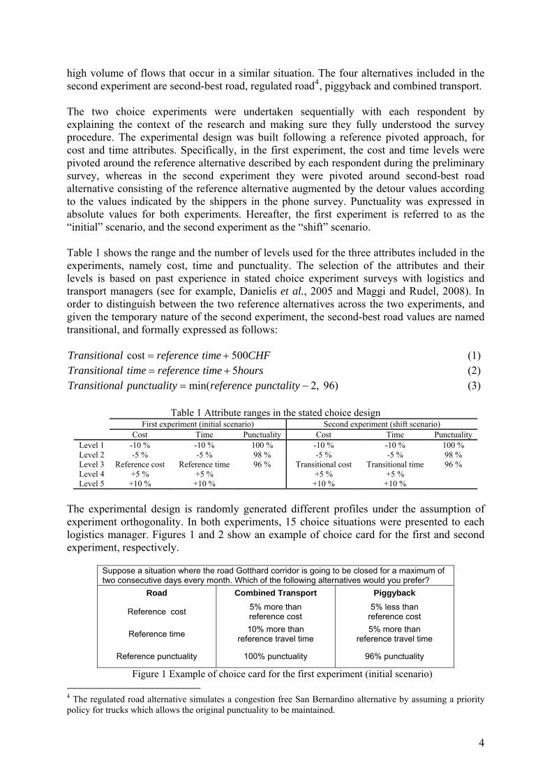
The experimental design is randomly generated different profiles under the assumption of experiment orthogonality. In both experiments, 15 choice situations were presented to each logistics manager. Figures 1 and 2 show an example of choice card for the first and second experiment, respectively.

Suppose a situation where the road Gotthard corridor is going to be closed for a maximum of two consecutive days every month. Which of the following alternatives would you prefer?

Road Combined Transport Piggyback

Reference cost 5% more than reference cost

5% less than reference cost

Reference time 10% more than reference travel time

5% more than reference travel time

Reference punctuality 100% punctuality 96% punctuality

Figure 1 Example of choice card for the first experiment (initial scenario) 4 The regulated road alternative simulates a congestion free San Bernardino alternative by assuming a priority policy for trucks which allows the original punctuality to be maintained.

4

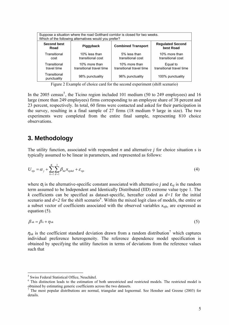
Suppose a situation where the road Gotthard corridor is closed for two weeks. Which of the following alternatives would you prefer?

Second best Road Piggyback Combined Transport Regulated Second

best Road

Transitional cost

10% less than transitional cost

5% less than transitional cost

10% more than transitional cost

Transitional travel time

10% more than transitional travel time

10% more than transitional travel time

Equal to transitional travel time

Transitional punctuality 98% punctuality 96% punctuality 100% punctuality

Figure 2 Example of choice card for the second experiment (shift scenario) In the 2005 census5, the Ticino region included 101 medium (50 to 249 employees) and 16 large (more than 249 employees) firms corresponding to an employee share of 38 percent and 23 percent, respectively. In total, 60 firms were contacted and asked for their participation in the survey, resulting in a final sample of 27 firms (18 medium 9 large in size). The two experiments were completed from the entire final sample, representing 810 choice observations. 3. Methodology The utility function, associated with respondent n and alternative j for choice situation s is typically assumed to be linear in parameters, and represented as follows:

2

1 1

K

njs j kd njskd njsk d

U xα β= =

= + +∑∑ ε (4)

where αj is the alternative-specific constant associated with alternative j and εnj is the random term assumed to be Independent and Identically Distributed (IID) extreme value type 1. The k coefficients can be specified as dataset-specific, hereafter coded as d=1 for the initial scenario and d=2 for the shift scenario6. Within the mixed logit class of models, the entire or a subset vector of coefficients associated with the observed variables xnjk, are expressed as equation (5).

nk k nkβ β η= + (5) ηnk is the coefficient standard deviation drawn from a random distribution7 which captures individual preference heterogeneity. The reference dependence model specification is obtained by specifying the utility function in terms of deviations from the reference values such that

5 Swiss Federal Statistical Office, Neuchâtel. 6 This distinction leads to the estimation of both unrestricted and restricted models. The restricted model is obtained by estimating generic coefficients across the two datasets. 7 The most popular distributions are normal, triangular and lognormal. See Hensher and Greene (2003) for details.

5

2 2 2

1 1 1 1 1 1

( ) ( ) ( ) ( )K K P

npd npnjs j nkd njskd nkd njskd njsk d k d p d

U dec x dec inc x inc zα β β= = = = = =

= + + + +∑∑ ∑∑ ∑∑φ ε

2

(6)

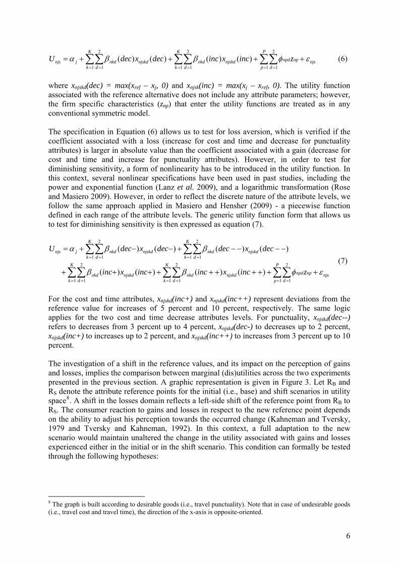
where xnjskd(dec) = max(xref – xj, 0) and xnjsk(inc) = max(xj – xref, 0). The utility function associated with the reference alternative does not include any attribute parameters; however, the firm specific characteristics (znp) that enter the utility functions are treated as in any conventional symmetric model. The specification in Equation (6) allows us to test for loss aversion, which is verified if the coefficient associated with a loss (increase for cost and time and decrease for punctuality attributes) is larger in absolute value than the coefficient associated with a gain (decrease for cost and time and increase for punctuality attributes). However, in order to test for diminishing sensitivity, a form of nonlinearity has to be introduced in the utility function. In this context, several nonlinear specifications have been used in past studies, including the power and exponential function (Lanz et al. 2009), and a logarithmic transformation (Rose and Masiero 2009). However, in order to reflect the discrete nature of the attribute levels, we follow the same approach applied in Masiero and Hensher (2009) - a piecewise function defined in each range of the attribute levels. The generic utility function form that allows us to test for diminishing sensitivity is then expressed as equation (7).

2 2

1 1 1 1

2 2

1 1 1 1 1 1

( ) ( ) ( ) ( )

( ) ( ) ( ) ( )

K K

njs j nkd njskd nkd njskdk d k d

K K P

npd npnkd njskd nkd njskd njsk d k d p d

U dec x dec dec x dec

inc x inc inc x inc z

α β β

β β φ

= = = =

= = = = = =

= + − − + − − − −

+ + + + + + + + + +

∑∑ ∑∑

∑∑ ∑∑ ∑∑ ε

(7)

For the cost and time attributes, xnjskd(inc+) and xnjskd(inc++) represent deviations from the reference value for increases of 5 percent and 10 percent, respectively. The same logic applies for the two cost and time decrease attributes levels. For punctuality, xnjskd(dec--) refers to decreases from 3 percent up to 4 percent, xnjskd(dec-) to decreases up to 2 percent, xnjskd(inc+) to increases up to 2 percent, and xnjskd(inc++) to increases from 3 percent up to 10 percent. The investigation of a shift in the reference values, and its impact on the perception of gains and losses, implies the comparison between marginal (dis)utilities across the two experiments presented in the previous section. A graphic representation is given in Figure 3. Let RB and RS denote the attribute reference points for the initial (i.e., base) and shift scenarios in utility space8. A shift in the losses domain reflects a left-side shift of the reference point from RB to RS. The consumer reaction to gains and losses in respect to the new reference point depends on the ability to adjust his perception towards the occurred change (Kahneman and Tversky, 1979 and Tversky and Kahneman, 1992). In this context, a full adaptation to the new scenario would maintain unaltered the change in the utility associated with gains and losses experienced either in the initial or in the shift scenario. This condition can formally be tested through the following hypotheses:

8 The graph is built according to desirable goods (i.e., travel punctuality). Note that in case of undesirable goods (i.e., travel cost and travel time), the direction of the x-axis is opposite-oriented.

6

Adaptation hypothesis (8) 0 2 1

0 2 1

" : ( ) (" : ( ) (

S B nk nk

S B nk nk

G G H inc incL L H dec dec

β ββ β

Δ = Δ → =⎧⎨Δ = Δ → =⎩

))

where the marginal utility (ΔGi) and marginal disutility (ΔLi), associated with a given attribute level in the gains and losses domains respectively, are identified as the coefficients associated with increases and decreases in the utility functions (6) and (7)9.

Figure 3 Adaptation Hypothesis

However, different reactions other than the adaptation hypothesis might occur if the individual has not completely adapted to the changed reference values. For example, we could expect a larger impact in the utility for gains in the shift scenario than in the initial scenario if the decision maker is trying to recover the initial loss. Formally,

Gains recovery hypothesis (9) 0 2 1

0 2 1

: ( ) ( ): ( ) (

S B nk nk

S B nk nk

G G H inc incL L H dec de

β ββ β

Δ > Δ → >⎧⎨Δ = Δ → =⎩ )c

Conversely, we might suppose a further increase in the loss aversion experienced from the decision maker as prevention to additional losses.

Additional losses prevention hypothesis (10) 0 2 1

0 2 1

: ( ) ( )

: ( ) ( )S B nk nk

S B nk nk

G G H inc incL L H dec dec

β ββ β

Δ = Δ → =⎧⎨Δ > Δ → >⎩

The estimation of the utility parameters associated with gains and losses, and their comparison across the two scenarios, allow us to test the hypotheses formulated, as well as any other pattern not discussed. Given the panel structure of the data collected from the two stated choice experiments and the use of the mixed logit class of models, the estimation of the utility parameters is derived from the maximization of the following simulated log likelihood:

1 exp( ' )lnexp( ' )

j n njs n nn

n r s j n njs n nj

LLR

′+ +=

′+ +∑ ∑ ∏ ∑α β x φ zα β x φ z

(11)

where s = 1, …, S represent the number of choice situations whereas r = 1, …, R refers to the number of draws. Within the Random Utility Model framework, the coefficients are

9 The introduction of nonlinearity in the utility functions does not alter the logic of the hypotheses assumed.

7

estimated along with the scale parameter, which reflects the variance of the unobserved component of the utility. Since different data sets have potentially different variances for unobserved utility, the comparison of the magnitude of the coefficients is possible only if the scale difference between the two data sets is taken into account. In this context, several techniques have been proposed in order to cope with difference in scale in jointly estimated choice models that use revealed preferences (RP) and stated preferences (SP) data (see for example, Swait and Louviere, 1993; Hensher and Bradley, 1993; Ben-Akiva and Morikawa, 1997). In this paper we refer to the approach recently used by Hensher (2008) which takes into account difference in scale by estimating the scale parameter for one of the two datasets considered in the pooled data10. According to Bhat and Castelar (2002), the scale parameter is expressed as follows:

,[(1 ) ]njs njs SPi j njs SPi,λ δ λ δ= − + i = 1, 2 (12) where ,njs SPiδ is a dummy variable that takes the value 1 for the observations associated with the dataset with the scale parameter normalised to 1, and zero otherwise. The parameter jλ is derivable by introducing in one of the two data sets (arbitrarily selected) a set of alternative-specific constants (ASC) that have a zero mean and free variance (Brownstone et al., 2000). In fact, the following relation holds:

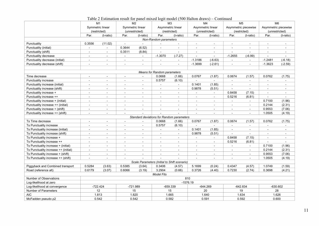
6 1.28255j ASCj ASCjλ π σ σ= = (13) where ASCjσ are the standard deviations of the alternative-specific constants introduced in data set i. In our case we estimate the scale parameter associated with the first data set, referring to the initial scenario, consisting of three alternatives, two hypothetical alternatives and the reference alternative respectively. From a preliminary analysis we noticed that the ASCs associated with the two hypothetical alternatives were not statistically different to one another. We decided then to nest the two hypothetical alternatives by constraining the estimation of only two additional ASCs, one for the reference alternative, and the other for the two hypothetical alternatives.11 4. Model Results We estimated three pairs of panel mixed logit models using 500 Halton draws12 with results summarised in Table 2. The first pair of models (M1 and M2) refers to linear symmetric specifications given in equation (4); that is the classic form of specification commonly used in discrete choice modeling. We then introduce the reference dependence models M3 and M4 defined in equation (6) that allows us to test for loss aversion. The last pair of models (M5 and M6) is of the form in equation (7), and still based on the reference dependence specification, but with the integration of attribute piecewise transformations in order to

10 It should be noted that in our context the aim is different from a typical RP and SP joint estimation. We are not interested to enrich the data with additional and complementary information, but we are instead looking at the comparison of coefficient magnitudes from different datasets. 11 Note that assuming different variance among alternatives is like imposing a nesting structure. In our case, we recognize a three levels nest structure. 12 See Train (2003) for details about Halton sequence. All models were estimated using a pre-release version of Nlogit 5.

8

9

capture potential nonlinearities that are compatible with the diminishing sensitivity prospect theory assumption. The difference within each pair of models is that the first model has generic-specific coefficient estimates (a restricted model), whereas in the second model the coefficients are treated as dataset-specific (an unrestricted model). This allows us to obtain an immediate, but overall, test on the hypothesis of adaptation by comparing the model fits within each pair of models. In terms of goodness of fit we report the log-likelihood at convergence, the McFadden pseudo ρ2 and the Akaike’s Information Criterion (AIC) (normalised for sample size) (see Table 2,). The best model in explaining the data is model M6 which reports a McFadden pseudo ρ2 of 0.600 and an AIC index of 1.626 versus a McFadden pseudo ρ2 of 0.542 and an ACI index of 1.820 obtained for model M2 which shows the poorest model fit measures among the six models estimated. Introducing nonlinearity in the reference dependence specification (models M5 and M6) increases, in general, the goodness of model fits in respect to the linear asymmetric specifications (models M3 and M4), and both specifications outperform substantially the symmetric ones (models M1 and M2). This trend confirms what was already experienced by Masiero and Hensher (2009) who analyse loss aversion and diminishing sensitivity using a subset of the present dataset (the initial scenario dataset). However, a first interesting result is provided from the comparison, within the three pairs of models, of the AIC index which in its calculation account for both a reduction in the log-likelihood and an increase in the number of parameters estimated. According to the AIC index, model M1 is preferred to M2, suggesting that there are no overall significant differences between the coefficients associated with the initial and shift scenarios. We observe exactly the opposite result once we introduce the reference dependence specifications, where models M4 and M6 outperform models M3 and M5 respectively. For each of the six models, we have estimated the scale parameters for the three alternatives associated with the initial scenario, with the aim of levelling any unobserved variance difference between the two datasets, making possible the comparison between coefficient estimates. The scale parameters are statistically significant, excluding the one referring to the reference alternative in model M3 and that associated with the hypothetical alternatives in model M4. From the statistically significant scale parameters, we observe that they all are smaller than one (except the scale for the piggyback and combined transport alternatives in model M6 that is 1.19), suggesting a greater variance of the unobserved effects for the initial scenario than for the shift scenario. Although it is plausible to expect a difference in scale between two datasets we had no expectation about the magnitude associated with the stated preferences structure of the experiment in both scenarios. However, when pooling stated and revealed preference data, a common practice is to hypothesise that the stated preference data hold a greater part of unobserved variance, even if it is not always verified. In this context, Hensher (2008), for example, does not report any statistically significant differences between stated and revealed preferences in terms of scale parameters.

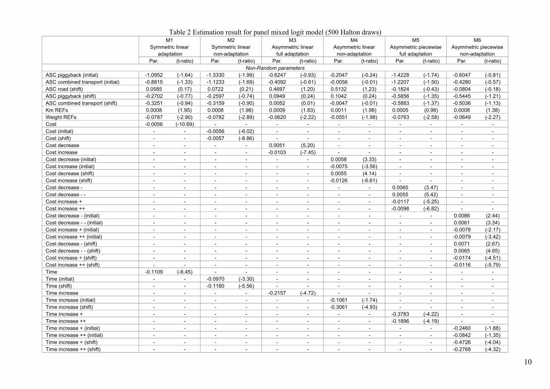
Table 2 Estimation result for panel mixed logit model (500 Halton draws) M1 M2 M3 M4 M5 M6 Symmetric linear Symmetric linear Asymmetric linear Asymmetric linear Asymmetric piecewise Asymmetric piecewise adaptation non-adaptation full adaptation non-adaptation full adaptation non-adaptation Par. (t-ratio) Par. (t-ratio) Par. (t-ratio) Par. (t-ratio) Par. (t-ratio) Par. (t-ratio)

Non-Random parameters ASC piggyback (initial) -1.0952 (-1.64) -1.3330 (-1.99) -0.6247 (-0.93) -0.2047 (-0.24) -1.4228 (-1.74) -0.6047 (-0.81) ASC combined transport (initial) -0.8815 (-1.33) -1.1233 (-1.69) -0.4092 (-0.61) -0.0056 (-0.01) -1.2207 (-1.50) -0.4280 (-0.57) ASC road (shift) 0.0585 (0.17) 0.0722 (0.21) 0.4697 (1.20) 0.5132 (1.23) -0.1824 (-0.43) -0.0804 (-0.18) ASC piggyback (shift) -0.2702 (-0.77) -0.2597 (-0.74) 0.0949 (0.24) 0.1042 (0.24) -0.5856 (-1.35) -0.5445 (-1.21) ASC combined transport (shift) -0.3251 (-0.94) -0.3159 (-0.90) 0.0052 (0.01) -0.0047 (-0.01) -0.5883 (-1.37) -0.5036 (-1.13) Km REFs 0.0008 (1.95) 0.0008 (1.98) 0.0009 (1.83) 0.0011 (1.98) 0.0005 (0.98) 0.0008 (1.38) Weight REFs -0.0787 (-2.90) -0.0782 (-2.89) -0.0620 (-2.22) -0.0551 (-1.98) -0.0763 (-2.58) -0.0649 (-2.27) Cost -0.0056 (-10.69) - - - - - - - - - - Cost (initial) - - -0.0056 (-6.02) - - - - - - - - Cost (shift) - - -0.0057 (-8.86) - - - - - - - - Cost decrease - - - - 0.0051 (5.20) - - - - - - Cost increase - - - - -0.0103 (-7.45) - - - - - - Cost decrease (initial) - - - - - - 0.0058 (3.33) - - - - Cost increase (initial) - - - - - - -0.0075 (-3.56) - - - - Cost decrease (shift) - - - - - - 0.0055 (4.14) - - - - Cost increase (shift) - - - - - - -0.0126 (-6.61) - - - - Cost decrease - - - - - - - - - 0.0065 (3.47) - - Cost decrease - - - - - - - - - - 0.0055 (5.42) - - Cost increase + - - - - - - - - -0.0117 (-5.25) - - Cost increase ++ - - - - - - - - -0.0098 (-6.82) - - Cost decrease - (initial) - - - - - - - - - - 0.0086 (2.44) Cost decrease - - (initial) - - - - - - - - - - 0.0061 (3.34) Cost increase + (initial) - - - - - - - - - - -0.0078 (-2.17) Cost increase ++ (initial) - - - - - - - - - - -0.0079 (-3.42) Cost decrease - (shift) - - - - - - - - - - 0.0071 (2.67) Cost decrease - - (shift) - - - - - - - - - - 0.0065 (4.65) Cost increase + (shift) - - - - - - - - - - -0.0174 (-4.51) Cost increase ++ (shift) - - - - - - - - - - -0.0116 (-5.79) Time -0.1109 (-6.45) - - - - - - - - - - Time (initial) - - -0.0970 (-3.30) - - - - - - - - Time (shift) - - -0.1180 (-5.56) - - - - - - - - Time increase - - - - -0.2157 (-4.72) - - - - - - Time increase (initial) - - - - - - -0.1061 (-1.74) - - - - Time increase (shift) - - - - - - -0.3061 (-4.93) - - - - Time increase + - - - - - - - - -0.3783 (-4.22) - - Time increase ++ - - - - - - - - -0.1896 (-4.19) - - Time increase + (initial) - - - - - - - - - - -0.2460 (-1.88) Time increase ++ (initial) - - - - - - - - - - -0.0842 (-1.35) Time increase + (shift) - - - - - - - - - - -0.4726 (-4.04) Time increase ++ (shift) - - - - - - - - - - -0.2768 (-4.32)

10

11

Table 2 Estimation result for panel mixed logit model (500 Halton draws) – Continued M1 M2 M3 M4 M5 M6 Symmetric linear Symmetric linear Asymmetric linear Asymmetric linear Asymmetric piecewise Asymmetric piecewise (restricted) (unrestricted) (restricted) (unrestricted) (restricted) (unrestricted) Par. (t-ratio) Par. (t-ratio) Par. (t-ratio) Par. (t-ratio) Par. (t-ratio) Par. (t-ratio)

Non-Random parameters Punctuality 0.3556 (11.02) - - - - - - - - - - Punctuality (initial) - - 0.3644 (6.52) - - - - - - - - Punctuality (shift) - - 0.3511 (8.84) - - - - - - - - Punctuality decrease - - - - -1.3070 (-7.27) - - -1.2655 (-6.99) - - Punctuality decrease (initial) - - - - - - -1.3186 (-6.63) - - -1.2481 (-6.18) Punctuality decrease (shift) - - - - - - -1.3699 (-2.61) - - -1.3623 (-2.59)

Means for Random parameters Time decrease - - - - 0.0668 (1.66) 0.0767 (1.87) 0.0674 (1.57) 0.0762 (1.75) Punctuality increase - - - - 0.5757 (6.10) - - - - - - Punctuality increase (initial) - - - - - - 0.1401 (1.85) - - - - Punctuality increase (shift) - - - - - - 0.9878 (5.51) - - - - Punctuality increase + - - - - - - - - 0.8458 (7.15) - - Punctuality increase ++ - - - - - - - - 0.5216 (6.81) - - Punctuality increase + (initial) - - - - - - - - - - 0.7100 (1.96) Punctuality increase ++ (initial) - - - - - - - - - - 0.2144 (2.31) Punctuality increase + (shift) - - - - - - - - - - 0.9553 (7.06) Punctuality increase ++ (shift) - - - - - - - - - - 1.0505 (4.19)

Standard deviations for Random parameters Ts Time decrease - - - - 0.0668 (1.66) 0.0767 (1.87) 0.0674 (1.57) 0.0762 (1.75) Ts Punctuality increase - - - - 0.5757 (6.10) - - - - - - Ts Punctuality increase (initial) - - - - - - 0.1401 (1.85) - - - - Ts Punctuality increase (shift) - - - - - - 0.9878 (5.51) - - - - Ts Punctuality increase + - - - - - - - - 0.8458 (7.15) - - Ts Punctuality increase ++ - - - - - - - - 0.5216 (6.81) - - Ts Punctuality increase + (initial) - - - - - - - - - - 0.7100 (1.96) Ts Punctuality increase ++ (initial) - - - - - - - - - - 0.2144 (2.31) Ts Punctuality increase + (shift) - - - - - - - - - - 0.9553 (7.06) Ts Punctuality increase ++ (shift) - - - - - - - - - - 1.0505 (4.19)

Scale Parameters (Initial to Shift scenario) Piggyback and Combined transport 0.5284 (3.63) 0.5385 (3.64) 0.3406 (4.57) 5.1699 (0.24) 0.4347 (4.57) 1.0749 (1.59) Road (reference alt) 0.6179 (3.07) 0.6066 (3.19) 3.2904 (0.66) 0.3726 (4.40) 0.7230 (2.74) 0.3698 (4.21)

Model FitsNumber of Observations 810 Log-likelihood at zero -1576.19 Log-likelihood at convergence -722.424 -721.989 -659.339 -644.269 -642.834 -630.602 Number of Parameters 12 15 15 20 19 28 AIC 1.813 1.820 1.665 1.640 1.634 1.626 McFadden pseudo ρ2 0.542 0.542 0.582 0.591 0.592 0.600

Looking at the parameter estimates that are in common to all the six models, we notice substantial homogeneity in the alternative-specific constants and the two firm-specific characteristics. Given that the ASC for the reference alternative is normalised to zero in both the initial and shift scenarios, the results show a negative propensity to switch towards rail-based alternatives, while the only other road alternative proposed in the experiments shows a positive sign for models M1 to M4, and a negative sign for models M5 and M6. However, most ASCs are not statistically significant at the alpha level of 0.10, with the exception of the constants referring to the initial scenario and those associated with the piggyback alternative in models M1, M2 and M3 and combined transport in model M2. The firm-specific variables are introduced in the utility of the two reference alternatives without distinguishing between the scenarios, since no significant differences were found from preliminary modelling. The first variable refers to the origin-destination distance (Km REFs) and shows a positive relationship between the reference alternative and travel distance. On the contrary, the firm-specific variable that refers to the weight of the transport (Weight REFs), indicates a preference of hypothetical alternatives proportional to the weight of the shipment. Turning to the coefficient estimates associated with the three modal attributes, namely cost, time and punctuality, all of the coefficients are of the expected sign and statistically significant. Models M1 and M2 show negative signs for cost and time and positive signs for punctuality, whereas models M3, M4, M5 and M6 report signs of the coefficients consistent with the definition of gains and losses around the reference point, where gains are associated with positive signs and losses with negative signs. For models M3 to M6, a further subset of random parameters has been estimated13 involving the coefficients associated with gains in both time and punctuality, that is time decrease and punctuality increase respectively. Since we are interested in comparing the means of the coefficients between the two scenarios, the inclusion of random parameters has been mainly focused on model fits, making sure of the exact identification of the parameter’s mean estimates14. The random parameters are distributed according to a triangular distribution; we constrained the standard deviation to be equal to the mean to ensure the same sign of the coefficient within the distribution (see Hensher and Greene, 2003 for proofs and discussions on the use of constrained triangular distribution in discrete choice models). As shown in Table 2, the coefficient associated with gains in time (time decrease) does not distinguish the initial and shift scenarios in models M4 and M6 and diminishing sensitivity in model M6. These constraints were necessary due to the statistical insignificance reported. Furthermore, we do not allow for nonlinearity in the loss domain of punctuality (punctuality decrease in models M5 and M6) due to the restriction imposed by the design for the shift scenario (see section 2). Indeed, it was possible to estimate nonlinearity in the initial scenario, but for the sake of comparison it has been treated as asymmetric, but linear, in both scenarios. Analyzing the magnitude of the parameters associated with gains and losses in models with reference dependence specifications (M3, M4, M5 and M6), we notice that all the parameter means associated with losses are in absolute values greater than those referring to gains. This holds for both initial and shift scenarios, supporting the assumption that respondents actually experienced loss aversion. Indeed, evidence of loss aversion has been found by other recent studies and in different contexts (see for example, Hess et al., 2008; De Borger and Fosgerau, 2008; Lanz et al., 2009; Rose and Masiero, 2009). From models M5 and M6, we can also 13 Note that the ASCs introduced in order to estimate the scale parameters are actually random parameters with zero mean and normal standard deviation. 14 As an identification test, each model has been run with 500 and 1000 Halton assuring the stability of both model fits and coefficients magnitude.

12

investigate the presence of diminishing sensitivity by comparing the magnitude of the coefficients estimated within the gains and losses domains for different attribute levels. Diminishing sensitivity is clearly evident in model M5 for all the three attributes considered, where the absolute values of the coefficients decrease as the attribute levels increase. This pattern is still present in model M6, although some linearity is experienced for the cost coefficients associated with losses in the initial scenario, and for the punctuality coefficients associated with gains in the shift scenario. The main focus of the paper is to investigate respondents’ behavioural changes in response to a shift in the reference values. In this context, we continue the analysis by performing a set of asymptotic t-ratio tests on the parameter estimates obtained for the unrestricted models M4 and M6, which allow us to test the hypotheses formulated in (8) - (10). Formally, the asymptotic t-ratio test is defined, according to the null hypotheses, as follow:

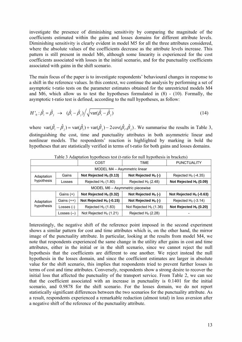
0ˆ ˆ ˆ ˆ ˆ ˆ' : ( ) var( )i j i j i jH β β β β β= → − − β (14)

where ˆ ˆ ˆ ˆ ˆ ˆvar( ) var( ) var( ) 2cov( , )i j i j i jβ β β β β− = + − β . We summarise the results in Table 3, distinguishing the cost, time and punctuality attributes in both asymmetric linear and nonlinear models. The respondents’ reaction is highlighted by marking in bold the hypotheses that are statistically verified in terms of t-ratio for both gains and losses domains.

Table 3 Adaptation hypotheses test (t-ratio for null hypothesis in brackets) COST TIME PUNCTUALITY

MODEL M4 – Asymmetric linear

Adaptation hypothesis

Gains Not Rejected H0 (0.13) Not Rejected H0 (-) Rejected H0 (-4.35)

Losses Rejected H0 (1.80) Rejected H0 (2.48) Not Rejected H0 (0.09)

MODEL M6 – Asymmetric piecewise

Adaptation hypothesis

Gains (+) Not Rejected H0 (0.32) Not Rejected H0 (-) Not Rejected H0 (-0.63) Gains (++) Not Rejected H0 (-0.15) Not Rejected H0 (-) Rejected H0 (-3.14)

Losses (-) Rejected H0 (1.83) Not Rejected H0 (1.36) Not Rejected H0 (0.20) Losses (--) Not Rejected H0 (1.21) Rejected H0 (2.28) -

Interestingly, the negative shift of the reference point imposed in the second experiment shows a similar pattern for cost and time attributes which is, on the other hand, the mirror image of the punctuality attribute. In particular, looking at the results from model M4, we note that respondents experienced the same change in the utility after gains in cost and time attributes, either in the initial or in the shift scenario, since we cannot reject the null hypothesis that the coefficients are different to one another. We reject instead the null hypothesis in the losses domain, and since the coefficient estimates are larger in absolute value for the shift scenario, this implies that respondents tried to prevent further losses in terms of cost and time attributes. Conversely, respondents show a strong desire to recover the initial loss that affected the punctuality of the transport service. From Table 2, we can see that the coefficient associated with an increase in punctuality is 0.1401 for the initial scenario, and 0.9878 for the shift scenario. For the losses domain, we do not report statistically significant differences between the two scenarios for the punctuality attribute. As a result, respondents experienced a remarkable reduction (almost total) in loss aversion after a negative shift of the reference of the punctuality attribute.

13

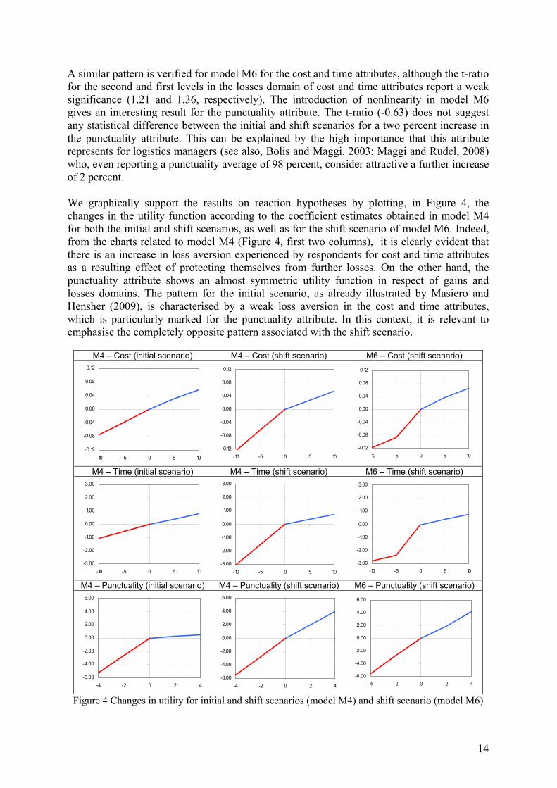
A similar pattern is verified for model M6 for the cost and time attributes, although the t-ratio for the second and first levels in the losses domain of cost and time attributes report a weak significance (1.21 and 1.36, respectively). The introduction of nonlinearity in model M6 gives an interesting result for the punctuality attribute. The t-ratio (-0.63) does not suggest any statistical difference between the initial and shift scenarios for a two percent increase in the punctuality attribute. This can be explained by the high importance that this attribute represents for logistics managers (see also, Bolis and Maggi, 2003; Maggi and Rudel, 2008) who, even reporting a punctuality average of 98 percent, consider attractive a further increase of 2 percent. We graphically support the results on reaction hypotheses by plotting, in Figure 4, the changes in the utility function according to the coefficient estimates obtained in model M4 for both the initial and shift scenarios, as well as for the shift scenario of model M6. Indeed, from the charts related to model M4 (Figure 4, first two columns), it is clearly evident that there is an increase in loss aversion experienced by respondents for cost and time attributes as a resulting effect of protecting themselves from further losses. On the other hand, the punctuality attribute shows an almost symmetric utility function in respect of gains and losses domains. The pattern for the initial scenario, as already illustrated by Masiero and Hensher (2009), is characterised by a weak loss aversion in the cost and time attributes, which is particularly marked for the punctuality attribute. In this context, it is relevant to emphasise the completely opposite pattern associated with the shift scenario.

M4 – Cost (initial scenario) M4 – Cost (shift scenario) M6 – Cost (shift scenario)

-0.12

-0.08

-0.04

0.00

0.04

0.08

0.12

-10 -5 0 5 10

-0.12

-0.08

-0.04

0.00

0.04

0.08

0.12

-10 -5 0 5 10

-0.12

-0.08

-0.04

0.00

0.04

0.08

0.12

-10 -5 0 5 10

M4 – Time (initial scenario) M4 – Time (shift scenario) M6 – Time (shift scenario)

-3.00

-2.00

-1.00

0.00

1.00

2.00

3.00

-10 -5 0 5 10

-3.00

-2.00

-1.00

0.00

1.00

2.00

3.00

-10 -5 0 5 10

-3.00

-2.00

-1.00

0.00

1.00

2.00

3.00

-10 -5 0 5 10

M4 – Punctuality (initial scenario) M4 – Punctuality (shift scenario) M6 – Punctuality (shift scenario)

-6.00

-4.00

-2.00

0.00

2.00

4.00

6.00

-4 -2 0 2 4

-6.00

-4.00

-2.00

0.00

2.00

4.00

6.00

-4 -2 0 2 4

-6.00

-4.00

-2.00

0.00

2.00

4.00

6.00

-4 -2 0 2 4

Figure 4 Changes in utility for initial and shift scenarios (model M4) and shift scenario (model M6)

14

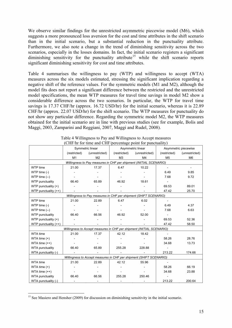
We observe similar findings for the unrestricted asymmetric piecewise model (M6), which suggests a more pronounced loss aversion for the cost and time attributes in the shift scenario than in the initial scenario, but a substantial reduction in the punctuality attribute. Furthermore, we also note a change in the trend of diminishing sensitivity across the two scenarios, especially in the losses domains. In fact, the initial scenario registers a significant diminishing sensitivity for the punctuality attribute15 while the shift scenario reports significant diminishing sensitivity for cost and time attributes. Table 4 summarises the willingness to pay (WTP) and willingness to accept (WTA) measures across the six models estimated, stressing the significant implication regarding a negative shift of the reference values. For the symmetric models (M1 and M2), although the model fits does not report a significant difference between the restricted and the unrestricted model specifications, the mean WTP measures for travel time savings in model M2 show a considerable difference across the two scenarios. In particular, the WTP for travel time savings is 17.37 CHF/hr (approx. 16.72 USD/hr) for the initial scenario, whereas it is 22.89 CHF/hr (approx. 22.07 USD/hr) for the shift scenario. The WTP measures for punctuality do not show any particular difference. Regarding the symmetric model M2, the WTP measures obtained for the initial scenario are in line with previous studies (see for example, Bolis and Maggi, 2003, Zamparini and Reggiani, 2007, Maggi and Rudel, 2008).

Table 4 Willingness to Pay and Willingness to Accept measures (CHF/hr for time and CHF/percentage point for punctuality)

Symmetric linear Asymmetric linear Asymmetric piecewise (restricted) (unrestricted) (restricted) (unrestricted) (restricted) (unrestricted) M1 M2 M3 M4 M5 M6

Willingness to Pay measures in CHF per shipment (INITIAL SCENARIO) WTP time 21.00 17.37 6.47 10.22 - - WTP time (-) - - - - 6.49 9.85 WTP time (--) - - - - 7.68 9.72 WTP punctuality 66.40 65.89 46.92 18.61 - WTP punctuality (+) - - - - 69.53 89.01 WTP punctuality (++) - - - - 47.42 25.70

Willingness to Pay measures in CHF per shipment (SHIFT SCENARIO) WTP time 21.00 22.89 6.47 6.02 - WTP time (-) - - - - 6.49 4.37 WTP time (--) - - - - 7.68 6.63 WTP punctuality 66.40 66.56 46.92 52.00 - WTP punctuality (+) - - - - 69.53 52.36 WTP punctuality (++) - - - - 47.42 58.50

Willingness to Accept measures in CHF per shipment (INITIAL SCENARIO) WTA time 21.00 17.37 42.12 18.42 - WTA time (+) - - - - 58.26 28.76 WTA time (++) - - - - 34.68 13.73 WTA punctuality 66.40 65.89 255.28 228.88 - WTA punctuality (-) - - - - 213.22 174.66

Willingness to Accept measures in CHF per shipment (SHIFT SCENARIO) WTA time 21.00 22.89 42.12 55.96 - WTA time (+) - - - - 58.26 66.19 WTA time (++) - - - - 34.68 23.88 WTA punctuality 66.40 66.56 255.28 250.46 - WTA punctuality (-) - - - - 213.22 200.64

15 See Masiero and Hensher (2009) for discussion on diminishing sensitivity in the initial scenario.

15

As investigated in previous studies (see for example, Hess et al., 2008; Lanz et al., 2009; Masiero and Hensher, 2009) the WTP decrease drastically when the utility function is specified according to the reference dependence assumption, which allows us to take into account for the WTA/WTP discrepancy (see, Horowitz and McConnell, 2002 for a review). Focusing on model M4, the initial scenario indicates a WTP for travel time savings of 10.22 CHF/hr and a WTA of 18.42 CHF/hr, setting the WTA/WTP ratio at 1.80, whereas we observe a WTP of 6.02 CHF/hr and a WTA of 55.96 CHF/hr for the shift scenario, which results in a ratio of 9.29. A similar structure for the WTP and WTA for travel time is outlined by model M6, although the diminishing sensitivity reported for time and cost attributes reveals a larger WTA/WTP discrepancy in the proximity of the reference values, both within and across the initial and shift scenarios. The consequence of a negative shift of the reference point suggests, therefore, a significant and substantial increase of the WTA/WTP ratio for travel time, where respondents experienced a lower WTP and a higher WTA with respect to the initial scenario. Reflecting the reaction hypotheses, the behavioural response to a negative shift of the reference value in terms of WTP and WTA for transport service punctuality shows an opposite pattern. In fact, the WTA/WTP discrepancy exhibits a general reduction passing from a ratio of 12.29 for the initial scenario in model M4 to 4.81 for the shift scenario. It is interesting to note the change in the respondents’ behaviour highlighted by the introduction of nonlinearity in model M6. In this case, for the initial scenario, the WTP for punctuality is particularly high for an increase of two percentage points (89.01 CHF/percentage point), but decrease dramatically for larger increases (25.70 CHF/percentage point), reflecting the very high sample median of 98 percent for the reference transport service. Nevertheless, we observe a levelling of these two values for the shift scenario (52.36 and 58.50 CHF/percentage point, respectively) which imposed a reduction of two percentage points over the reference alternative values. 5. Conclusions This paper has investigated the reaction experienced by decision makers facing a negative shift of the reference point within a reference pivoted stated choice experiment framework. The analysis has been based on two choice experiments conducted amongst logistics managers, and collected in Switzerland in 2008. The experiments were designed to identify the indirect freight transport costs associated with a temporary closure of the main reference road alternative. The first experiment reflected the initial conditions, and hence was designed around the typical (or initial) reference alternative. We then introduced the hypothesis of road closure and updated the initial reference alternative values according to the second best road alternative (shifted or expected reference alternative) values which were then used to pivot the design of the second stated choice experiment. Under an assumption of prospect theory, a change in the reference point affects the structure of individuals’ preferences. In order to investigate any potential reaction within the sample interviewed, we pooled the data from the two experiments and estimated three pairs of models. Within each pair of models, the distinction has been made by performing the restricted and unrestricted model specifications, where the restriction involved the specification of generic coefficients across the two datasets. The first pair of models assumed a symmetric specification. We introduced the reference dependence specification in the second pair of models, and estimated linear asymmetric parameters for both gains and losses. In the third pair of models, we further allowed for asymmetric nonlinearity in gains and

16

losses domains by estimating, through a piecewise transformation, different parameters for different attribute levels. The model results for the two reference-dependent specifications indicate that respondents experienced a significant reaction when facing a a negative shift of the reference point. The unrestricted version of the models outperforms the restricted one, providing significant support to the prospect theory assumption regarding the alteration of respondent preference structure. From a comparison of the parameter estimates, we observed that respondents, on average, increased their loss aversion for cost and time attributes reflecting a willingness to prevent further losses. On the contrary, for the punctuality attribute, we registered a decrease in the loss aversion due to a considerable increase in the marginal utility associated with gains reasonably explained as the propensity to recover the initial loss. These results not only confirm the priority of the punctuality attribute within the logistics managers’ choice of freight transport services but also indicate that a small decrease in the punctuality quality has a high impact on preference formation, even for a limited timeframe, as supposed in our study. The results obtained for the symmetric specifications do not indicate any statistically significant reaction in terms of model performance. We note therefore a clear difficulty of the classic economic theory in capturing changes in behaviour under a shift reference point context, although this is not surprising given the symmetric structure of these specifications. The estimates of WTP and WTA measures from the reference dependence models report a WTA substantially higher than the WTP, which is in line with expectations. Comparing the two scenarios, the results suggest that a negative shift of the reference point causes a reduction in the WTP and an increase in the WTA for travel time, and an overall increase of the WTP, and a slight increase of the WTA for transport service punctuality. The significance of the differences in terms of WTP and WTA measures across the two scenarios is a relevant finding. Policy makers should therefore consider the consumers potential reactions in any context involving a shift of the reference point. In particular, we think about reference pivoted stated choice experiments studying the introduction of toll roads or congestion pricing schemes in general. In these cases, particular attention should be addressed to the specification of the reference values. Further research is suggested in order to support these findings in different contexts. Given that our study was based on a shift of the reference point in the short run and limited in time, we recognise the relevance of these findings in choices affecting everyday life concerning transitional road detours for infrastructures maintenance, and we advise the implementation of cost benefit analysis studies in this direction. However, we also suggest the need for further investigation in a context involving a permanent shift of the reference point, such as the introduction of pricing schemes. Finally, the analysis of a positive shift of the reference point would be of interest in order to support recent findings (e.g., Arkes et al. 2008), noting that individuals tend to adapt more completely to gains (positive shifts) than to losses (negative shifts).

17

References Arkes, H.R., Hirshleifer, D, Jiang, D., Lim, S., 2008. Reference Point Adaptation: Tests in the Domain of Security Trading. Organizational Behavior and Human Decision Processes, 105, 67-81. Bhat, C.R., Castelar, S., 2002. A unified mixed logit framework for modeling revealed and stated preferences: formulation and application to congestion pricing analysis in the San Francisco Bay area. Transportation Research Part B 36, 577–669. Ben-Akiva, M., Bradley M., Morikawa T., Benjamin J., Novak T., Oppewal H., Rao V., 1994. Combining revealed and stated preferences data. Marketing Letters 5(4), 335-349. Bolis, S., Maggi R., 2003. Logistics Strategy and Transport Service Choices-An Adaptive Stated Preference Experiment. In: Growth and Change - A journal of Urban and Regional Policy, Special Issue STELLA FG 1, (34) 4. Brownstone, D., Bunch, D.S., Train, K., 2000. Joint mixed logit models of stated and revealed preferences for alternative-fuel vehicles. Transportation Research Part B 34, 315–338. Danielis, R., Marcucci, E., Rotaris, L., 2005. Logistics managers' stated preferences for freight service attributes. Transportation Research Part E 41(3), 201-215. De Borger, B., Fosgerau, M., 2008. The trade-off between money and travel time: a test of the theory of reference-dependent preferences. Journal of Urban Economics 64, 101-115. Hensher, D.A., 2008. Empirical approaches to combining revealed and stated preference data: Some recent developments with reference to urban mode choice. Research in transportation Economics 23, 23-29. Hensher, D.A., Bradley, M., 1993. Using stated response data to enrich revealed preference discrete choice models. Marketing Letters 4(2), 139-152. Hensher, D.A., Greene, W.H., 2003. Mixed logit models: state of practice. Transportation 30(2), 133-176. Hess, S. and Rose, J.M. (2009) Should reference alternatives in pivot design SC surveys be treated differently? Transportation Research Board Annual Meeting, Washington DC, January. Hess, S., Rose, J.M., Hensher, D.A., 2008. Asymmetric preference formation in willingness to pay estimates in discrete choice models. Transportation Research Part E 44(5), 847-863. Horowitz, J., McConnell, K.E., 2002. A Review of WTA-WTP Studies. Journal of Environmental Economics and Management 44, 426-47. Kahneman, D., Tversky A., 1979. Prospect Theory: an analysis of decision under risk. Econometrica 47 (2), 263–291.

18

Lanz, B., Provins, A., Bateman, I., Scarpa, R., Willis, K., Ozdemiroglu, E., 2009. Investigating willingness to pay – willingness to accept asymmetry in choice experiments. Paper selected for presentation at the International Choice Modelling Conference 2009, Leeds (UK). Maggi, R., Rudel, R., 2008. The Value of Quality Attributes in Freight Transport: Evidence from an SP-Experiment in Switzerland. In: Ben-Akiva, M.E., Meersman, H., van de Voorde E. (Eds.), Recent Developments in Transport Modelling. Emerald Group Publishing Limited. Maggi, R., Masiero, L., Baruffini, M., Thu�ring M., 2009. Evaluation of the optimal resilience for vulnerable infrastructure networks. An interdisciplinary pilot study on the transalpine transportation corridors. Swiss National Science Foundation, NRP 54 “Sustainable Development of the Built Environment”, Project 405 440, Final Scientific Report. Masiero, L., Hensher, D.A., 2009. Analyzing loss aversion and diminishing sensitivity in a freight transport stated choice experiment. Institute of Transport and Logistics Studies, University of Sydney, July. Masiero, L., Maggi, R., 2009. Estimation of indirect cost and evaluation of protective measures for infrastructure vulnerability: A case study on the transalpine transport corridor. Istituto Ricerche Economiche, University of Lugano, September. McFadden, D., 1974. Conditional logit analysis of qualitative choice behavior. In: Zarembka, P. (Ed.), Frontiers in Econometrics. Academic Press, New York. Rose, J.M., Bliemer, M.C.J., Hensher, D.A., Collins, A.T., 2008. Designing efficient stated choice experiments in the presence of reference alternatives. Transportation Research Part B 42(4), 395-406. Rose, J.M., Masiero, L., 2009. A comparison of prospect theory in WTP and preference space. Institute of Transport and Logistics Studies, University of Sydney, October. Schwartz, A., Goldberg, J., Hazen, G., 2008. Prospect theory, reference points, and health decisions. Judgement and Decision Making 3(2), 174-180. Swait, J., Louviere, J.J., 1993. The role of the scale parameter in the estimation and comparison of multinomial logit models. Journal of Marketing Research 30(3), 305-314. Train, K., 2003. Discrete Choice Methods with Simulation. Cambridge University Press, Cambridge. Tversky, A., Kahneman, D., 1991. Loss aversion in riskless choice: A reference-dependent model. Quarterly Journal of Economics 106, 1039-1061. Tversky A., Kahneman, D., 1992. Advances in Prospect Theory: Cumulative Representation of Uncertainty. Journal of Risk and Uncertainty 5, 297-323.

19

20

Zamparini, L., Reggiani, A., 2007. The value of travel time in passenger and freight transport: An overview. In: van Geenhuizen, M., Reggiani, A., Rietveld, P. (Eds.), Policy analysis of transport networks. Ashgate, Aldershot.

QUADERNI DELLA FACOLTÀ

1998:

P. Balestra, Efficient (and parsimonious) estimation of structural dynamic error component models

1999:

M. Filippini, Cost and scale efficiency in the nursing home sector : evidence from Switzerland L. Bernardi, I sistemi tributari di oggi : da dove vengono e dove vanno L.L. Pasinetti, Economic theory and technical progress G. Barone-Adesi, K. Giannopoulos, L. Vosper, VaR without correlations for portfolios of derivative securities G. Barone-Adesi, Y. Kim, Incomplete information and the closed-end fund discount G. Barone-Adesi, W. Allegretto, E. Dinenis, G. Sorwar, Valuation of derivatives based on CKLS interest rate models M. Filippini, R. Maggi, J. Mägerle, Skalenerträge und optimale Betriebsgrösse bei den schweizerische Privatbahnen E. Ronchetti, F. Trojani, Robust inference with GMM estimators G.P. Torricelli, I cambiamenti strutturali dello sviluppo urbano e regionale in Svizzera e nel Ticino sulla base dei dati dei censimenti federali delle aziende 1985, 1991 e 1995

2000:

E. Barone, G. Barone-Adesi, R. Masera, Requisiti patrimoniali, adeguatezza del capitale e gestione del rischio G. Barone-Adesi, Does volatility pay? G. Barone-Adesi, Y. Kim, Incomplete information and the closed-end fund discount R. Ineichen, Dadi, astragali e gli inizi del calcolo delle probabilità W. Allegretto, G. Barone-Adesi, E. Dinenis, Y. Lin, G. Sorwar, A new approach to check the free boundary of single factor interest rate put option G.D.Marangoni, The Leontief Model and Economic Theory B. Antonioli, R, Fazioli, M. Filippini, Il servizio di igiene urbana italiano tra concorrenza e monopolio L. Crivelli, M. Filippini, D. Lunati. Dimensione ottima degli ospedali in uno Stato federale L. Buchli, M. Filippini, Estimating the benefits of low flow alleviation in rivers: the case of the Ticino River L. Bernardi, Fiscalità pubblica centralizzata e federale: aspetti generali e il caso italiano attuale M. Alderighi, R. Maggi, Adoption and use of new information technology F. Rossera, The use of log-linear models in transport economics: the problem of commuters’ choice of mode

2001: M. Filippini, P. Prioni, The influence of ownership on the cost of bus service provision in Switzerland. An empirical illustration B. Antonioli, M. Filippini, Optimal size in the waste collection sector B. Schmitt, La double charge du service de la dette extérieure L. Crivelli, M. Filippini, D. Lunati, Regulation, ownership and efficiency in the Swiss nursing home industry S. Banfi, L. Buchli, M. Filippini, Il valore ricreativo del fiume Ticino per i pescatori L. Crivelli, M. Filippini, D. Lunati, Effizienz der Pflegeheime in der Schweiz

2002: B. Antonioli, M. Filippini, The use of a variable cost function in the regulation of the Italian water industry B. Antonioli, S. Banfi, M. Filippini, La deregolamentazione del mercato elettrico svizzero e implicazioni a breve termine per l’industria idroelettrica M. Filippini, J. Wild, M. Kuenzle, Using stochastic frontier analysis for the access price regulation of electricity networks G. Cassese, On the structure of finitely additive martingales

2003: M. Filippini, M. Kuenzle, Analisi dell’efficienza di costo delle compagnie di bus italiane e svizzere C. Cambini, M. Filippini, Competitive tendering and optimal size in the regional bus transportation industry L. Crivelli, M. Filippini, Federalismo e sistema sanitario svizzero L. Crivelli, M. Filippini, I. Mosca, Federalismo e spesa sanitaria regionale : analisi empirica per i Cantoni svizzeri M. Farsi, M. Filippini, Regulation and measuring cost efficiency with panel data models : application to electricity distribution utilities M. Farsi, M. Filippini, An empirical analysis of cost efficiency in non-profit and public nursing homes F. Rossera, La distribuzione dei redditi e la loro imposizione fiscale : analisi dei dati fiscali svizzeri L. Crivelli, G. Domenighetti, M. Filippini, Federalism versus social citizenship : investigating the preference for equity in health care M. Farsi, Changes in hospital quality after conversion in ownership status G. Cozzi, O. Tarola, Mergers, innovations, and inequality M. Farsi, M. Filippini, M. Kuenzle, Unobserved heterogeneity in stochastic cost frontier models : a comparative analysis

2004: G. Cassese, An extension of conditional expectation to finitely additive measures S. Demichelis, O. Tarola, The plant size problem and monopoly pricing F. Rossera, Struttura dei salari 2000 : valutazioni in base all’inchiesta dell’Ufficio federale di statistica in Ticino M. Filippini, M. Zola, Economies of scale and cost efficiency in the postal services : empirical evidence from Switzerland F. Degeorge, F. Derrien, K.L. Womack, Quid pro quo in IPOs : why book-building is dominating auctions M. Farsi, M. Filippini, W. Greene, Efficiency measurement in network industries : application to the Swiss railway companies L. Crivelli, M. Filippini, I. Mosca, Federalism and regional health care expenditures : an empirical analysis for the Swiss cantons S. Alberton, O. Gonzalez, Monitoring a trans-border labour market in view of liberalization : the case of Ticino M. Filippini, G. Masiero, K. Moschetti, Regional differences in outpatient antibiotic consumption in Switzerland A.S. Bergantino, S. Bolis, An adaptive conjoint analysis of freight service alternatives : evaluating the maritime option

2005: M. Farsi, M. Filippini, An analysis of efficiency and productivity in Swiss hospitals M. Filippini, G. Masiero, K. Moschetti, Socioeconomic determinants of regional differences in outpatient antibiotic consumption : evidence from Switzerland

2006: M. Farsi, L. Gitto, A statistical analysis of pain relief surgical operations M. Farsi, G. Ridder, Estimating the out-of-hospital mortality rate using patient discharge data S. Banfi, M. Farsi, M. Filippini, An empirical analysis of child care demand in Switzerland L. Crivelli, M. Filippini, Regional public health care spending in Switzerland : an empirical analysis M. Filippini, B. Lepori, Cost structure, economies of capacity utilization and scope in Swiss higher education institutions M. Farsi, M. Filippini, Effects of ownership, subsidization and teaching activities on hospital costs in Switzerland M. Filippini, G. Masiero, K. Moschetti, Small area variations and welfare loss in the use of antibiotics in the community A. Tchipev, Intermediate products, specialization and the dynamics of wage inequality in the US A. Tchipev, Technological change and outsourcing : competing or complementary explanations for the rising demand for skills during the 1980s?

2007: M. Filippini, G. Masiero, K. Moschetti, Characteristics of demand for antibiotics in primary care : an almost ideal demand system approach G. Masiero, M. Filippini, M. Ferech, H. Goossens, Determinants of outpatient antibiotic consumption in Europe : bacterial resistance and drug prescribers R. Levaggi, F. Menoncin, Fiscal federalism, patient mobility and the soft budget constraint : a theoretical approach M. Farsi, The temporal variation of cost-efficiency in Switzerland’s hospitals : an application of mixed models

2008:

Quaderno n. 08-01

M. Farsi, M. Filippini, D. Lunati, Economies of scale and efficiency measurement in Switzerland’s nursing homes

Quaderno n. 08-02

A. Vaona, Inflation persistence, structural breaks and omitted variables : a critical view

Quaderno n. 08-03

A. Vaona, The sensitivity of non parametric misspecification tests to disturbance autocorrelation

Quaderno n. 08-04

A. Vaona, STATA tip : a quick trick to perform a Roy-Zellner test for poolability in STATA

Quaderno n. 08-05

A. Vaona, R. Patuelli, New empirical evidence on local financial development and growth

Quaderno n. 08-06

C. Grimpe, R. Patuelli, Knowledge production in nanomaterials : an application of spatial filtering to regional system of innovation

Quaderno n. 08-07

A. Vaona, G. Ascari, Regional inflation persistence : evidence from Italy

Quaderno n. 08-08

M. Filippini, G. Masiero, K. Moschetti, Dispensing practices and antibiotic use

Quaderno n. 08-09

T. Crossley, M. Jametti, Pension benefit insurance and pension plan portfolio choice

Quaderno n. 08-10

R. Patuelli, A. Vaona, C. Grimpe, Poolability and aggregation problems of regional innovation data : an application to nanomaterial patenting

Quaderno n. 08-11

J.H.L. Oud, H. Folmer, R. Patuelli, P. Nijkamp, A spatial-dependence continuous-time model for regional unemployment in Germany

2009:

Quaderno n. 09-01

J.G. Brida, S. Lionetti, W.A. Risso, Long run economic growth and tourism : inferring from Uruguay

Quaderno n. 09-02

R. Patuelli, D.A. Griffith, M. Tiefelsdorf, P. Nijkamp, Spatial filtering and eigenvector stability : space-time models for German unemployment data

Quaderno n. 09-03

R. Patuelli, A. Reggiani, P. Nijkamp, N. Schanne, Neural networks for cross-sectional employment forecasts : a comparison of model specifications for Germany

Quaderno n. 09-04

A. Cullmann, M. Farsi, M. Filippini, Unobserved heterogeneity and International benchmarking in public transport

Quaderno n. 09-05

M. Jametti, T. von Ungern-Sternberg, Hurricane insurance in Florida

Quaderno n. 09-06

S. Banfi, M. Filippini, Resource rent taxation and benchmarking : a new perspective for the Swiss hydropower sector

Quaderno n. 09-07

S. Lionetti, R. Patuelli, Trading cultural goods in the era of digital piracy

Quaderno n. 09-08

M. Filippini, G. Masiero, K. Moschetti, Physician dispensing and antibiotic prescriptions

2010:

Quaderno n. 10-01

R. Patuelli, N. Schanne, D.A. Griffith, P. Nijkamp, Persistent disparities in regional unemployment : application of a spatial filtering approach to local labour markets in Germany

Quaderno n. 10-02

K. Deb, M. Filippini, Public bus transport demand elasticities in India

Quaderno n. 10-03

L. Masiero, R. Maggi, Estimation of indirect cost and evaluation of protective measures for infrastructure vulnerability : a case study on the transalpine transport corridor

Quaderno n. 10-04

L. Masiero, D.A. Hensher, Analyzing loss aversion and diminishing sensitivity in a freight transport stated choice experiment

Quaderno n. 10-05

L. Masiero, D.A. Hensher, Shift of reference point and implications on behavioral reaction to gains and losses