Embed Size (px)
Citation preview

THE UNIVERSITY OF ADELAIDE
Faculty of Sciences
Shelf-Life:Designing and Analysing
Stability Trials
A thesis submitted for the degree of
Doctor of Philosophy
by
Andreas Kiermeier
December 2003

Abstract
All pharmaceutical products are required by law to display an expiry date on the packag-
ing. The period between the date of manufacture and expiry date is known as the label
shelf-life. The label shelf-life indicates the period of time during which the consumer can
expect the product to be safe and effective.
Methods for determining the label shelf-life from stability data are discussed in the guide-
lines on the evaluation of stability data issued by the International Conference for Har-
monization. These methods are limited to data that can be analysed using linear model
methods. Furthermore, in the situation where a number of batches are used to determine
a label shelf-life, the current regulatory method (unintentionally) penalizes good statisti-
cal design. In addition, the label shelf-life obtained this way may not be a reliable guide
to the properties of future batches produced under similar conditions.
In this thesis it is shown that the current definition of the label shelf-life may not provide
the consumer with the desired level of confidence that the product is safe and effective.
This is especially the case when the manufacturer has performed a well designed stability
study with many assays. Consequently, a new definition for the label shelf-life is proposed,
such that the consumer can be confident that a certain percentage of the product will
meet the specification by the expiry date. Several methods for obtaining such a label
shelf-life under linear model and generalized linear model assumptions are proposed and
evaluated using simulation studies.
The new definition of label shelf-life is extended to allow a label shelf-life to be obtained
from stability studies that make use of many batches, such that a proportion of product
i

over all batches can be assured to meet specifications by the expiry date. Several methods
for estimating the label shelf-life in the multi-batch case are proposed and evaluated with
the help of simulation studies.
ii

Declaration
This work contains no material which has been accepted for the award of any other degree
or diploma in any university or other tertiary institution and, to the best of my knowledge
and belief, contains no material previously published or written by another person, except
where due reference has been made in the text.
I give consent to this copy of my thesis, when deposited in the University Library, being
available for loan and photocopying.
Signed: Date:
iii

Acknowledgements
I wish to thank my supervisors Assoc. Prof. Arunas P. Verbyla and Dr. Richard G.
Jarrett for their support, guidance and friendship during this research.
iv

Contents
Abstract i
Declaration iii
Acknowledgements iv
1 Introduction 1
1.1 Label Shelf-life Estimation for a Single Batch . . . . . . . . . . . . . . . . 2
1.2 Testing for Batch-to-Batch Variability . . . . . . . . . . . . . . . . . . . . 9
1.3 Label Shelf-life Estimation for Multiple Batches . . . . . . . . . . . . . . . 11
1.3.1 The Fixed Effects Model: Current Regulatory Guidelines . . . . . . 12
1.3.2 The Random Effects Model . . . . . . . . . . . . . . . . . . . . . . 15
1.4 Addressing the Issues . . . . . . . . . . . . . . . . . . . . . . . . . . . . . . 18
2 Estimation of Shelf-Life: The Single Batch Case 20
2.1 A New Definition . . . . . . . . . . . . . . . . . . . . . . . . . . . . . . . . 20
2.2 Estimation of the Label Shelf-Life . . . . . . . . . . . . . . . . . . . . . . . 23
2.2.1 Normal Approximation . . . . . . . . . . . . . . . . . . . . . . . . . 24
2.2.2 Various Profile Likelihood Based Approaches . . . . . . . . . . . . . 26
2.2.3 Constrained Profile Likelihood (CPL) Based Approaches . . . . . . 37
2.2.4 Non-central t-distribution (NCT) Approach . . . . . . . . . . . . . 45
2.3 Simulation Results . . . . . . . . . . . . . . . . . . . . . . . . . . . . . . . 46
2.4 Discussion . . . . . . . . . . . . . . . . . . . . . . . . . . . . . . . . . . . . 70
v
CONTENTS
3 Estimation of Shelf-Life: The Multi-Batch Case 74
3.1 A New Definition . . . . . . . . . . . . . . . . . . . . . . . . . . . . . . . . 74
3.2 Estimation of the Label Shelf-Life . . . . . . . . . . . . . . . . . . . . . . . 78
3.2.1 Normal Approximation . . . . . . . . . . . . . . . . . . . . . . . . . 79
3.2.2 Various Profile Likelihood Based Approaches . . . . . . . . . . . . . 82
3.2.3 Constrained Profile Likelihood Based Approaches . . . . . . . . . . 88
3.2.4 Non-central t-distribution (NCT) Approach . . . . . . . . . . . . . 91
3.3 Simulation Results . . . . . . . . . . . . . . . . . . . . . . . . . . . . . . . 94
3.4 Discussion . . . . . . . . . . . . . . . . . . . . . . . . . . . . . . . . . . . . 115
4 Estimation of Shelf-Life: The GLM Single Batch Case 118
4.1 Introduction . . . . . . . . . . . . . . . . . . . . . . . . . . . . . . . . . . . 118
4.2 Likelihood based approaches . . . . . . . . . . . . . . . . . . . . . . . . . . 121
4.2.1 Constrained Profile Likelihood . . . . . . . . . . . . . . . . . . . . . 122
4.2.2 Example: The Normal Distribution . . . . . . . . . . . . . . . . . . 125
4.2.3 Example: The Gamma Distribution . . . . . . . . . . . . . . . . . . 128
4.3 Simulation Results . . . . . . . . . . . . . . . . . . . . . . . . . . . . . . . 132
4.3.1 The Normal Distribution . . . . . . . . . . . . . . . . . . . . . . . . 132
4.3.2 The Gamma Distribution . . . . . . . . . . . . . . . . . . . . . . . 133
4.4 Discussion . . . . . . . . . . . . . . . . . . . . . . . . . . . . . . . . . . . . 142
5 Conclusions 144
5.1 Other Applications . . . . . . . . . . . . . . . . . . . . . . . . . . . . . . . 145
5.2 Future Work . . . . . . . . . . . . . . . . . . . . . . . . . . . . . . . . . . . 147
vi
CHAPTER 1
Introduction
Pharmaceutical companies are required by law to indicate the expiry date of each phar-
maceutical product on the immediate container. This expiry date indicates the end of
the period of time, known as shelf-life, during which the product can be expected to
meet specifications. The guidelines which govern how the label shelf-life, and hence the
expiry date, is determined are set out by the International Conference on Harmonisation
(ICH) of Technical Requirements for Registration of Pharmaceuticals for Human Use
(ICH, 2003; , 2002). These guidelines are adopted by the regulatory authorities of the
European Union, Japan and the USA. Other countries also adopt these guidelines with
little or no modification.
Before a product can be released to the market, manufacturers need to apply for a label
shelf-life to the appropriate authority — the Therapeutic Goods Administration (TGA)
in Australia and the Food and Drug Administration (FDA) in the United States. The
label shelf-life is only granted if the manufacturer can demonstrate that the product will
remain within specifications during that period. After approval, the degradation of the
product must also be monitored to ensure that the shelf-life remains appropriate. These
requirements are usually achieved by storing the product under suitable conditions and
monitoring the degradation. This type of study is referred to as a stability study.
General overviews of the analysis of stability data are given in Kohberger (1988), Lin
1
1.1. LABEL SHELF-LIFE ESTIMATION FOR A SINGLE BATCH
(1990), Buncher and Tsay (1993), and Chow and Liu (1995b), while Carstensen and Rhodes
(2000) give an overview which is more focused on the development of drug products. The
ICH guidelines attempt to give guidance on analysing stability data, and while several
areas covered in these guidelines have received further attention in the literature, there
are still problems with these recommendations. These include the estimation of a label
shelf-life for a single batch, testing for variability between batches, and the estimation of
a label shelf-life which is applicable to all future batches. These three areas are reviewed
below.
1.1 Label Shelf-life Estimation for a Single Batch
Long term stability studies are typically carried out after approval for a new drug product
has been given, but they can also be run as part of a new drug application. In long term
stability studies the expectation is that the drug product remains within specifications for
at least 12 months after manufacture. The ICH (2003) suggests that testing is performed
every three months during the first year, every six months during the second year, and on
an annual basis thereafter. Denote the testing times by x1, . . . , xN and the corresponding
assay results by y1, . . . , yN , where N is the total number of assays. These assay results
may be expressed as a percentage of the claimed label amount and log transformed if
necessary (ICH, 2003). While sampling times are not all required to be distinct, assay
results are assumed to be independent.
An appropriate statistical model for the degradation relationship may take the form
yi = xTi β + ei , (1.1)
or in matrix notation
y = Xβ + e ,
where
• yi is the response from the i-th assay for i = 1, . . . , N , on the arithmetic or loga-
rithmic scale, and y is the column vector of yi’s,
2
1.1. LABEL SHELF-LIFE ESTIMATION FOR A SINGLE BATCH
• xTi , the i-th row of the design matrix X, is a p-dimensional predictor vector corre-
sponding to the i-th response,
• β is a p-dimensional vector of fixed effects, and
• ei are independently and identically distributed (i.i.d.) normal errors, with mean 0
and variance σ2, and e is the column vector of ei’s.
The responses yi will hereinafter be referred to as potency, but they could equally refer
to any other measurement.
The current definition of shelf-life (ICH, 2003) is
“the time interval that a drug product is expected to remain within the approved
shelf-life specification provided that it is stored under the conditions defined on
the label in the proposed containers and closure”.
This definition is equivalent to the mathematical definition for the true shelf-life of a single
batch (Chow and Shao, 1990; Shao and Chow, 1994), namely the time τ such that
τ = inf
t : xTt β ≤ κ
, (1.2)
where inf denotes the infimum or greatest lower bound, κ is the specification limit, or
acceptance criterion, and xt is the vector of regressors at time t. Note that a similar
definition applies to responses that increase with time.
Different ways of estimating the shelf-life have been proposed. Tatke (1980) used an
approach based on survival analysis which relied on a drug product having failed, that is,
having a potency less than the specification limit. Such an approach is of little practical
value since pharmaceutical companies usually require an estimate of the shelf-life long
before any of the products have actually failed. A more useful approach made use of
degradation measurements over time and fitted an L1 regression model to this degradation
data (Tapon, 1993). This method was chosen as being more robust than least squares
regression, which tends to be the method in the literature and regulatory guidelines.
3
1.1. LABEL SHELF-LIFE ESTIMATION FOR A SINGLE BATCH
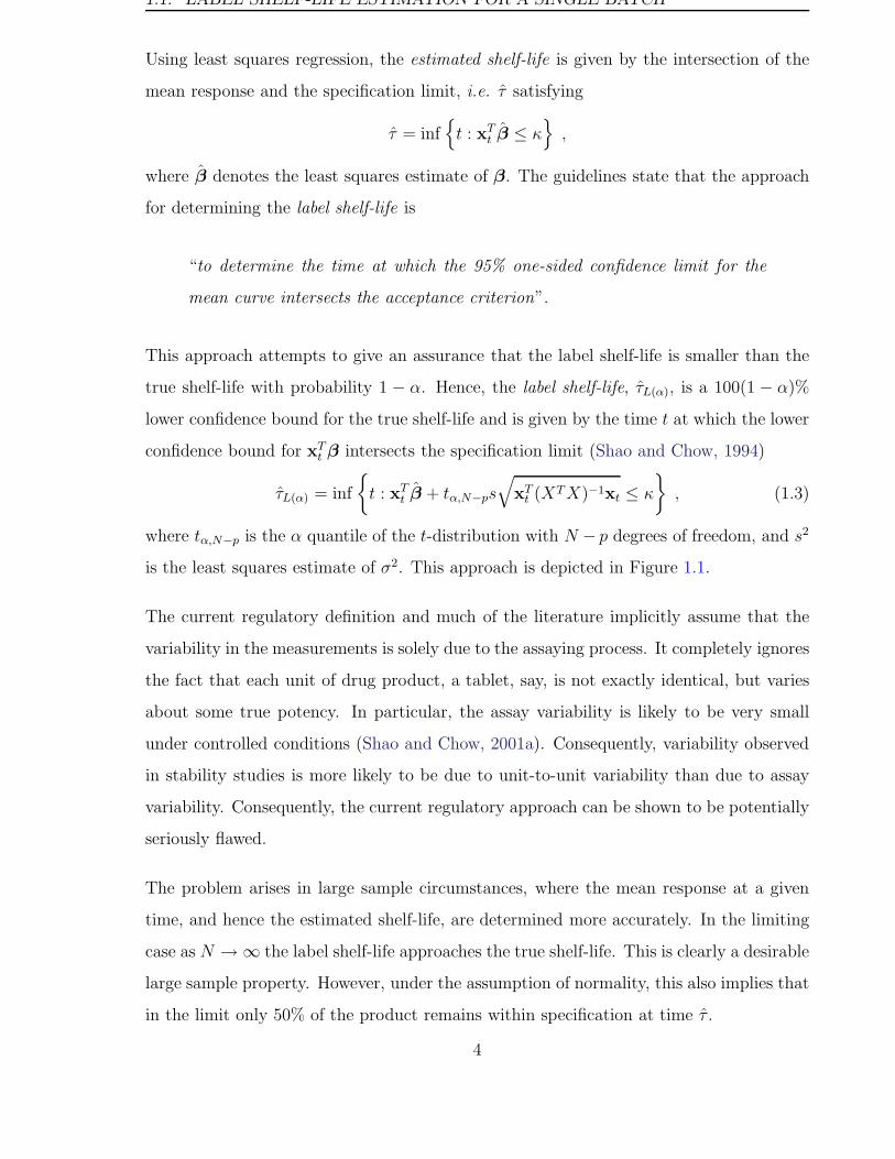
Using least squares regression, the estimated shelf-life is given by the intersection of the
mean response and the specification limit, i.e. τ satisfying
τ = inf
t : xTt β ≤ κ
,
where β denotes the least squares estimate of β. The guidelines state that the approach
for determining the label shelf-life is
“to determine the time at which the 95% one-sided confidence limit for the
mean curve intersects the acceptance criterion”.
This approach attempts to give an assurance that the label shelf-life is smaller than the
true shelf-life with probability 1 − α. Hence, the label shelf-life, τL(α), is a 100(1 − α)%
lower confidence bound for the true shelf-life and is given by the time t at which the lower
confidence bound for xTt β intersects the specification limit (Shao and Chow, 1994)
τL(α) = inf
t : xTt β + tα,N−ps
√
xTt (XTX)−1xt ≤ κ
, (1.3)
where tα,N−p is the α quantile of the t-distribution with N − p degrees of freedom, and s2
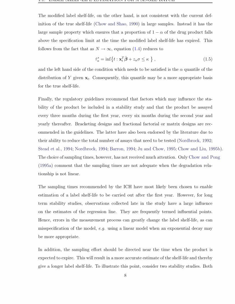
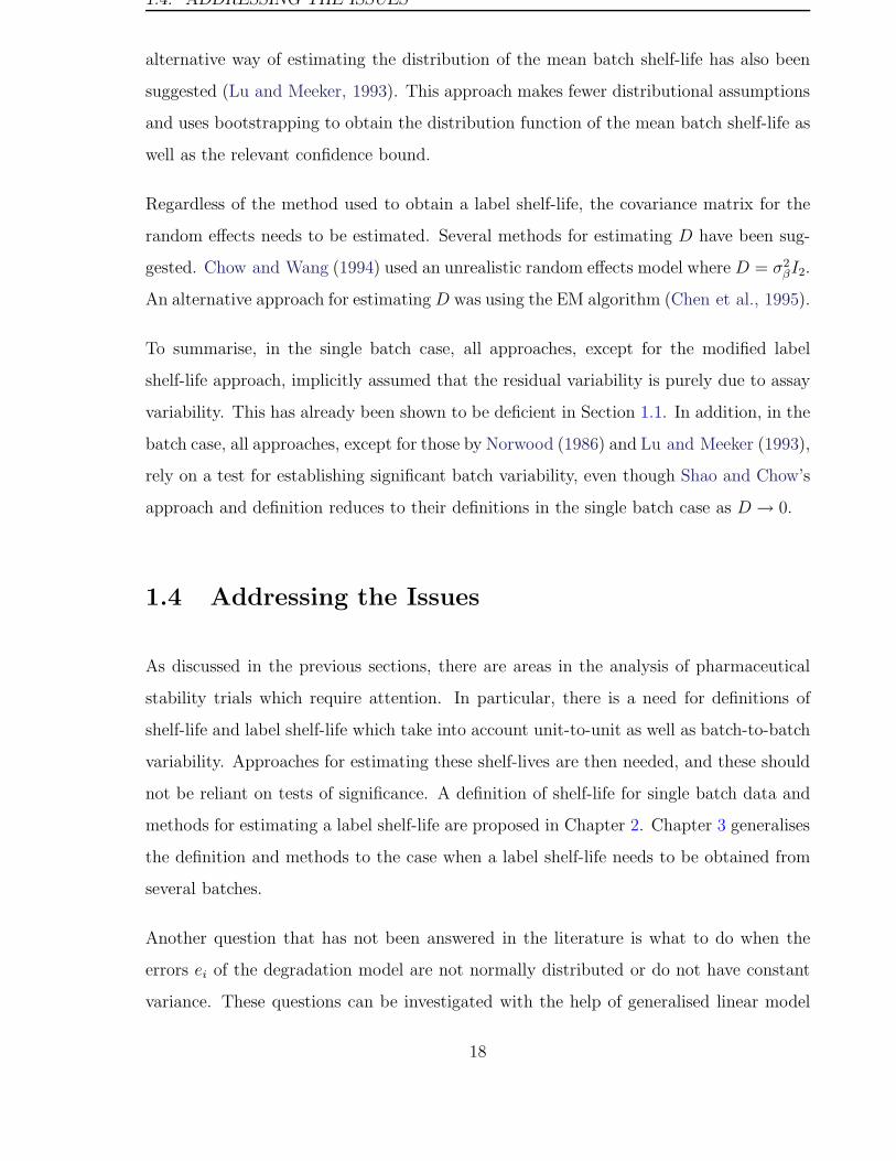
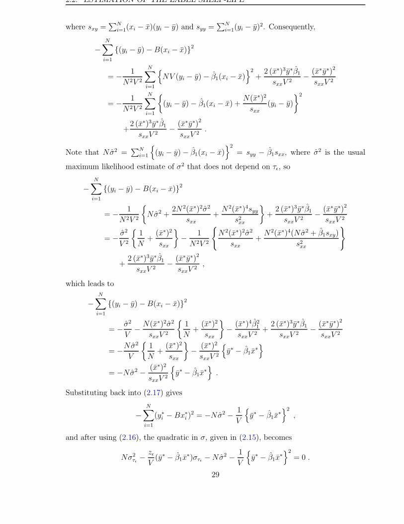
is the least squares estimate of σ2. This approach is depicted in Figure 1.1.
The current regulatory definition and much of the literature implicitly assume that the
variability in the measurements is solely due to the assaying process. It completely ignores
the fact that each unit of drug product, a tablet, say, is not exactly identical, but varies
about some true potency. In particular, the assay variability is likely to be very small
under controlled conditions (Shao and Chow, 2001a). Consequently, variability observed
in stability studies is more likely to be due to unit-to-unit variability than due to assay
variability. Consequently, the current regulatory approach can be shown to be potentially
seriously flawed.
The problem arises in large sample circumstances, where the mean response at a given
time, and hence the estimated shelf-life, are determined more accurately. In the limiting
case as N → ∞ the label shelf-life approaches the true shelf-life. This is clearly a desirable
large sample property. However, under the assumption of normality, this also implies that
in the limit only 50% of the product remains within specification at time τ .
4
1.1. LABEL SHELF-LIFE ESTIMATION FOR A SINGLE BATCH
0 5 10 15 20 25 30 35
8085
9095
100
Time (months)
% P
oten
cy o
f Lab
el C
laim
Regression LineLower 95% Conf. BoundSpecification Limit
ττL(α)
Figure 1.1: Current regulatory approach to estimating the shelf-life and the label shelf-life
using a linear regression model.
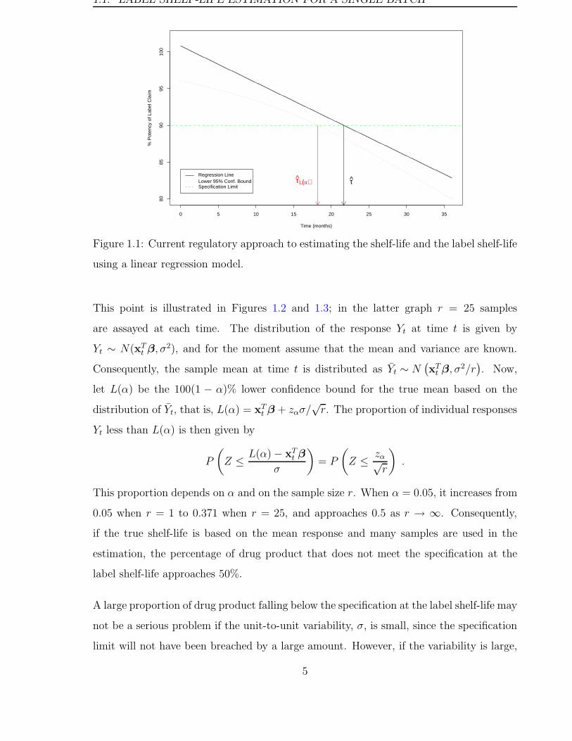
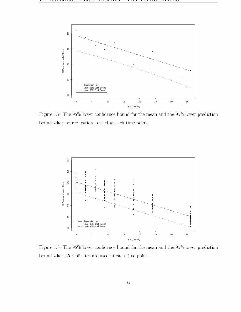
This point is illustrated in Figures 1.2 and 1.3; in the latter graph r = 25 samples
are assayed at each time. The distribution of the response Yt at time t is given by
Yt ∼ N(xTt β, σ2), and for the moment assume that the mean and variance are known.
Consequently, the sample mean at time t is distributed as Yt ∼ N(
xTt β, σ2/r
)
. Now,
let L(α) be the 100(1 − α)% lower confidence bound for the true mean based on the
distribution of Yt, that is, L(α) = xTt β + zασ/
√r. The proportion of individual responses
Yt less than L(α) is then given by
P
(
Z ≤ L(α) − xTt β
σ
)
= P
(
Z ≤ zα√r
)
.
This proportion depends on α and on the sample size r. When α = 0.05, it increases from
0.05 when r = 1 to 0.371 when r = 25, and approaches 0.5 as r → ∞. Consequently,
if the true shelf-life is based on the mean response and many samples are used in the
estimation, the percentage of drug product that does not meet the specification at the
label shelf-life approaches 50%.
A large proportion of drug product falling below the specification at the label shelf-life may
not be a serious problem if the unit-to-unit variability, σ, is small, since the specification
limit will not have been breached by a large amount. However, if the variability is large,
5
1.1. LABEL SHELF-LIFE ESTIMATION FOR A SINGLE BATCH
0 5 10 15 20 25 30 35
8085
9095
100
Time (months)
% P
oten
cy o
f Lab
el C
laim
Regression LineLower 95% Conf. BoundLower 95% Pred. Bound
Figure 1.2: The 95% lower confidence bound for the mean and the 95% lower prediction
bound when no replication is used at each time point.
0 5 10 15 20 25 30 35
8085
9095
100
105
110
Time (months)
% P
oten
cy o
f Lab
el C
laim
Regression LineLower 95% Conf. BoundLower 95% Pred. Bound
Figure 1.3: The 95% lower confidence bound for the mean and the 95% lower prediction
bound when 25 replicates are used at each time point.
6
1.1. LABEL SHELF-LIFE ESTIMATION FOR A SINGLE BATCH
then some products may fall far short of the specification. For products that increase in
toxicity, say, this relates to a large proportion of product exceeding a safe specification
limit. This may have serious consequences — even if the product is used within its
shelf-life.
An alternative approach, which overcomes these shortcomings, is based on the prediction
interval of a future observation (Carstensen and Nelson, 1976). Carstensen and Nelson
define what will be referred to as a modified label shelf-life, τ ∗L(α). This modified label
shelf-life is the time at which the 100(1 − α)% lower prediction bound intersects the
specification limit, that is,
τ ∗L(α) = inf
t : xTt β + tα,N−ps
√
1 + xTt (XTX)−1xt ≤ κ
. (1.4)
The prediction bound considers the distribution of a single future observation. Hence this
approach attempts to make a statement about the ability of an individual item (a tablet,
say) to meet the specifications at time t, rather than the ability of the mean of all items
of a batch to meet the specifications. This leads to a more conservative, that is, shorter
shelf-life.
Comparing the label shelf-life and the modified label shelf-life, in Figure 1.2, with r = 1,
the label shelf-life would be set at about 20 months, yet the same product in Figure 1.3,
with r = 25, would give a label shelf-life of about 24 months. However, using (1.4) would
lead to a modified label shelf-life of about 14 months in each case and would guarantee
that 95% of the product exceed the specifications at that time. Which label shelf-life is
used is clearly of importance to the consumer.
Another undesirable property of the current regulatory approach is the lack of influence
the product variability has on the definition of shelf-life and consequently on the estima-
tion process. In particular, since primary interest lies in the mean response, increasing
the number of samples can compensate for a manufacturing process with large unit-to-
unit variability σ2. This is often cheaper than attempting to improve the manufacturing
process, but it does not put enough emphasis on good manufacturing practices and com-
mitment to quality.
7
1.1. LABEL SHELF-LIFE ESTIMATION FOR A SINGLE BATCH
The modified label shelf-life, on the other hand, is not consistent with the current def-
inition of the true shelf-life (Chow and Shao, 1990) in large samples. Instead it has the
large sample property which ensures that a proportion of 1 − α of the drug product falls
above the specification limit at the time the modified label shelf-life has expired. This
follows from the fact that as N → ∞, equation (1.4) reduces to
τ ∗α = inf
t : xTt β + zασ ≤ κ
, (1.5)
and the left hand side of the condition which needs to be satisfied is the α quantile of the
distribution of Y given xt. Consequently, this quantile may be a more appropriate basis
for the true shelf-life.
Finally, the regulatory guidelines recommend that factors which may influence the sta-
bility of the product be included in a stability study and that the product be assayed
every three months during the first year, every six months during the second year and
yearly thereafter. Bracketing designs and fractional factorial or matrix designs are rec-
ommended in the guidelines. The latter have also been endorsed by the literature due to
their ability to reduce the total number of assays that need to be tested (Nordbrock, 1992;
Stead et al., 1994; Nordbrock, 1994; Barron, 1994; Ju and Chow, 1995; Chow and Liu, 1995b).
The choice of sampling times, however, has not received much attention. Only Chow and Pong
(1995a) comment that the sampling times are not adequate when the degradation rela-
tionship is not linear.
The sampling times recommended by the ICH have most likely been chosen to enable
estimation of a label shelf-life to be carried out after the first year. However, for long
term stability studies, observations collected late in the study have a large influence
on the estimates of the regression line. They are frequently termed influential points.
Hence, errors in the measurement process can greatly change the label shelf-life, as can
misspecification of the model, e.g. using a linear model when an exponential decay may
be more appropriate.
In addition, the sampling effort should be directed near the time when the product is
expected to expire. This will result in a more accurate estimate of the shelf-life and thereby
give a longer label shelf-life. To illustrate this point, consider two stability studies. Both
8
1.2. TESTING FOR BATCH-TO-BATCH VARIABILITY
are conducted on a product with a true shelf-life of 25 months. In each study the product
is sampled once at each of 8 times x1, . . . , x8. The first study follows the methodology of
the current guidelines (ICH, 2003). The sampling times xi are chosen to be 0, 3, 6, 9, 12,
18, 24, and 36 months. Consequently, the mean sampling time x equals 13.5 months and
the sum of squared deviations is sxx =∑8
i=1(xi − x)2 = 1008. This means that at the
true shelf-life, the margin of error m.e. used in the confidence interval of (1.2) is
m.e. = tα,6 × s×√
1
8+
(25 − 13.5)2
1008= tα,6 × s× 0.5062 ,
where tα,6 denotes the appropriate critical value from the t distribution with 6 degrees of
freedom, and s denotes the estimated standard deviation of the residuals.
On the other hand, the second study concentrates the sampling times near where the
shelf life is expected to be. The sampling frequency in the first and third year are simply
swapped such that the sampling times are 0, 12, 18, 24, 27, 30, 33 and 36. The value of the
mean sampling time now becomes 22.5 months while the value of sxx remains unchanged.
The margin of error becomes
m.e. = tα,6 × s× 0.3622 .
Consequently, the margin of error for the mean regression line can be reduced substantially
near where the shelf-life is expected to fall simply by choosing more appropriate sampling
times. This can be done without any additional sampling effort.
In order to better combine the objectives of early estimation and more accuracy near the
shelf-life, it is therefore recommended that stability testing be performed every three or
at most every six months. Over a period of three years, three-monthly testing results in
a margin of error equal to t∗ × s× 0.3269 while six monthly testing results in a margin of
error of t∗ × s× 0.4376.
1.2 Testing for Batch-to-Batch Variability
Pharmaceutical products are generally manufactured in batches. Ideally, these batches
are identical, but in practice, variation from batch to batch will be unavoidable. Different
9
1.2. TESTING FOR BATCH-TO-BATCH VARIABILITY
raw materials for example may be an important source of this variation.
Due to the time delay that is involved in the determination of a label shelf-life it is not
practical to wait until a label shelf-life is obtained for a batch before it is released onto
the market. In fact, as the ICH (2002) states:
“Where applicable, an appropriate statistical method should be employed to
analyze the long-term primary stability data in an original application. The
purpose of this analysis [of stability data] is to establish, with a high degree of
confidence, a retest period or shelf life during which a quantitative attribute will
remain within acceptance criteria for all future batches manufactured, pack-
aged, and stored under similar circumstances. This same method could also
be applied to commitment batches to verify or extend the originally approved
retest period or shelf life.”
The guidelines indicate that a minimum of three primary batches is required for stability
studies. The guidelines (ICH, 2003; , 2002) indicate that if batch-to-batch variability is
small then three batches can be analysed as one. This is established by testing for equality
of slopes and intercepts, using a significance level of 0.25. However, if significance tests
show that batches cannot be combined, then the label shelf-life should be based on the
minimum of the three label shelf-lives obtained from analysing each batch separately.
The choice of significance level of 0.25 is unusual, and has likely been chosen in order to
increase the power of the test (Ruberg and Stegeman, 1991). However, Ruberg and Hsu
(1990) correctly point out that “a penalty is paid for doing a good study, whereas a
poor study allows one to pool more batches into the shelf-life calculation”. Consequently,
they propose an approach that is analogous to one used for establishing bioequivalence
(Ruberg and Hsu, 1990; , 1992). This proposed test uses a “multiple comparison pro-
cedure with the worst” as a decision rule for combining batches. An alternative pro-
cedure, which is based on fixing the power of the test in advance, was proposed by
Ruberg and Stegeman (1991). Another approach is described by Yoshioka et al. (2002),
who calculate a shelf-life for each batch and then use the range of shelf-lives to decide
10
1.3. LABEL SHELF-LIFE ESTIMATION FOR MULTIPLE BATCHES
whether batches are significantly different from each other.
However, all these tests suffer from the same misconception — they treat batches as fixed
effects. It has been pointed out that the shelf-life, when estimated from a fixed effects
model, is not applicable to all future batches (Chow and Shao, 1989; Ho et al., 1992).
Consequently, the label shelf-life and any testing procedure should take random batch
variability into account. Three test procedures, which are all based on the assumption
that batches are random, are proposed by Chow and Shao (1989), and a further set of
tests was proposed by Chow and Shao (1990). All these methods test whether the random
effects covariance matrix is significantly different from zero.
Basing the type of analysis on the result of a significance test is referred to as a two
stage approach. While this two-stage approach appears sensible, it runs the risk, like
all statistical tests, of wrong conclusions. An attempt at establishing the effects of a
misspecified model was made by Lee and Cagon (1994). However, they used a model
which only allowed for the intercept to be random. Their results indicated that a fixed
effects model overestimates the shelf-life when there is random batch variability. Freeman
(1989) showed that, at least in the case of cross-over trials, “the two-stage analysis is too
misleading to be of practical use”. Consequently, an approach which incorporates random
batch variability into the definition of shelf-life is preferred over one that tests for the
significance of such variability.
1.3 Label Shelf-life Estimation for Multiple Batches
In the case that batch variability is shown to be significant, various approaches have
been suggested for the estimation of a label shelf-life. These approaches are based on
either a fixed or random effects model. The current regulatory guidelines only consider
the fixed effects model (ICH, 2002), which cannot be used to make statements about
future batches. The random effects model, which is a more realistic model, assumes that
batches are random, with some underlying distribution. Based on the random effects
model, probability statements about all future batches can then be made.
11

1.3. LABEL SHELF-LIFE ESTIMATION FOR MULTIPLE BATCHES
Both these models are now considered in turn.
1.3.1 The Fixed Effects Model: Current Regulatory Guidelines
In the situation when there is significant batch-to-batch variability, Shao and Chow (1994)
pointed out that the “minimum of three” approach lacks statistical justification. Since
batches are treated as fixed effects, conclusions drawn from the batches used in the stabil-
ity trial cannot be generalised to all future batches. This can only be achieved by treating
batches as random effects. At the same time, using more batches in the analysis can
result in the smallest estimate of shelf-life (obtained separately for each batch) becoming
smaller, possibly to some limit.
The statement about the lack of statistical justification is examined here with the help of
a simulation study. The simulations were structured as those in Section 3.3 of Chapter 3.
A summary of the structure is as follows.
• The number of batches k takes values 3, 4, 5, 6, 7, 8, 9, 10, 20 and 50.
• A random sample of k batch effects bj were drawn from N(β, D), where β =
(100,−0.3)T , D is a 2 × 2 matrix with diagonal elements equal to 1 and 0.003, and
off-diagonal elements equal to d2 = −0.03, 0 or 0.03. This allows for negative, no
and positive correlation between the intercepts and slopes.
• A random sample of size r = 1 was drawn for each batch at times xi = 0, 3, 6, 9, 12,
18, 24 and 36 from the distribution N(xTi bj, σ2), where xT
i = (1, xi) and σ2 = 0.52.
• This was repeated 1000 times.
The restrictions on r and σ2 are made to better suit the approach taken in the regulatory
guidelines. Note that under the current definition, the true shelf-life is determined by
the time at which the mean degradation curve intersects the specification limit. In these
simulations the true shelf-life equals τ0.5 = (90 − 100)/(−0.3) = 33.3 months.
12
1.3. LABEL SHELF-LIFE ESTIMATION FOR MULTIPLE BATCHES
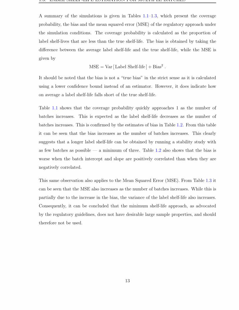
A summary of the simulations is given in Tables 1.1–1.3, which present the coverage
probability, the bias and the mean squared error (MSE) of the regulatory approach under
the simulation conditions. The coverage probability is calculated as the proportion of
label shelf-lives that are less than the true shelf-life. The bias is obtained by taking the
difference between the average label shelf-life and the true shelf-life, while the MSE is
given by
MSE = Var [ Label Shelf-life ] + Bias2 .
It should be noted that the bias is not a “true bias” in the strict sense as it is calculated
using a lower confidence bound instead of an estimator. However, it does indicate how
on average a label shelf-life falls short of the true shelf-life.
Table 1.1 shows that the coverage probability quickly approaches 1 as the number of
batches increases. This is expected as the label shelf-life decreases as the number of
batches increases. This is confirmed by the estimates of bias in Table 1.2. From this table
it can be seen that the bias increases as the number of batches increases. This clearly
suggests that a longer label shelf-life can be obtained by running a stability study with
as few batches as possible — a minimum of three. Table 1.2 also shows that the bias is
worse when the batch intercept and slope are positively correlated than when they are
negatively correlated.
This same observation also applies to the Mean Squared Error (MSE). From Table 1.3 it
can be seen that the MSE also increases as the number of batches increases. While this is
partially due to the increase in the bias, the variance of the label shelf-life also increases.
Consequently, it can be concluded that the minimum shelf-life approach, as advocated
by the regulatory guidelines, does not have desirable large sample properties, and should
therefore not be used.
13
1.3
.LA
BE
LSH
ELF-L
IFE
EST
IMA
TIO
NFO
RM
ULT
IPLE
BA
TC
HE
S
k 3 4 5 6 7 8 9 10 20 50
d2 = −0.03 0.964 0.982 0.997 0.998 0.999 1.000 1.000 1.000 1.000 1.000d2 = 0 0.959 0.978 0.992 0.997 0.997 1.000 1.000 1.000 1.000 1.000d2 = 0.03 0.936 0.979 0.992 0.997 1.000 0.998 1.000 1.000 1.000 1.000
Table 1.1: Coverage probabilities of the current regulatory approach as evaluated using a simulation study with β1 = −0.3 andσ = 0.5.
k 3 4 5 6 7 8 9 10 20 50
d2 = −0.03 -5.10 -6.13 -6.77 -6.88 -7.19 -7.41 -7.65 -7.79 -8.89 -9.91d2 = 0 -6.43 -7.47 -8.11 -8.58 -8.89 -9.23 -9.54 -9.66 -11.21 -12.69d2 = 0.03 -7.12 -8.23 -8.97 -10.00 -10.14 -10.58 -11.04 -11.08 -12.91 -14.61
Table 1.2: Bias of the current regulatory approach as evaluated using a simulation study with β1 = −0.3 and σ = 0.5.
k 3 4 5 6 7 8 9 10 20 50
d2 =−0.03 34.55 43.58 51.11 51.97 55.97 58.84 62.40 64.09 81.67 99.99d2 =0 56.34 66.95 74.58 82.00 85.81 92.15 97.38 99.84 129.92 163.88d2 =0.03 71.18 84.89 94.47 111.73 112.69 122.00 130.79 130.66 172.28 217.25
Table 1.3: Mean Squared Error of the current regulatory approach as evaluated using a simulation study with β1 = −0.3 andσ = 0.5.
14

1.3. LABEL SHELF-LIFE ESTIMATION FOR MULTIPLE BATCHES
1.3.2 The Random Effects Model
Random effects models have been considered by several authors in one form or another.
A general form which is frequently used is
Yij|bj = xTijbj + eij , (1.6)
where
• Yij denotes the i-th assay result from the j-th batch for i = 1, . . . , Nj and j =
1, . . . , k, on the arithmetic or logarithmic scale, such that the total number of ob-
servations is N =∑k
j=1Nj,
• xij is a p-dimensional predictor vector corresponding to the i-th observation from
the j-th batch,
• bj is a p-dimensional vector of random effects for the j-th batch, distributed as
bj ∼ N(β, D), and
• eij are i.i.d. errors independent of bj such that ej = (e1j, . . . , eNjj)T ∼ N(0, σ2Ij),
where Ij is the identity of size Nj .
The distribution of Yj = (Y1j , . . . , YNjj)T , conditional on bj , is then given by
Yj|bj ∼ N(
Xjbj , σ2Ij)
where Xj is the Nj × p model matrix of full rank for batch j, with xij in the i-th row.
Unconditionally,
Yj ∼ N (Xjβ,Σj) ,
where Σj = σ2Ij +XjDXTj . The joint unconditional distribution of all observations over
all batches is now given by
Y ∼ N (Xβ,Σ) , (1.7)
where Y = (YT1 . . .Y
Tk )T , X =
[
XT1 . . .X
Tk
]Tand Σ = diag(Σ1, . . . ,Σk). As usual, the
realization of Yij is denoted by yij, such that Yj and Y become yj and y, respectively.
15
1.3. LABEL SHELF-LIFE ESTIMATION FOR MULTIPLE BATCHES
It will be assumed hereafter that batches degrade linearly over time, in which case β =
(β0, β1)T , and
D =
d1 d2
d2 d3
.
This variance matrix for the bi describes the form of the underlying response from one
batch to another. The value of d1, the variance of b0j , describes how the average activity
varies from batch to batch at time t = 0, the time of manufacture; the value of d3, the
variance of b1j , describes how the rate of degradation varies from one batch to another;
and the value of the covariance d2 indicates how b0j affects b1j . That is, batches that
start with more active ingredient degrade faster if d2 < 0 and degrade slower when
d2 > 0. Consequently, positive values of d2 have the effect of increasing the variability
of the response at time t, where the variance of the response due to batch variation is
d1 + 2 d2t + d3t2. This is likely to lead to shorter label shelf-lives due to the greater
uncertainty.
Norwood (1986) considered a model with a random intercept, that is, bj = b0j and
b0j ∼ N(β0, d1), because the modified shelf-life (Carstensen and Nelson, 1976) does not
hold for models which included batch effects. Hence the unconditional distribution of Yj
is N(Xjβ,Σj), where Σj = σ2Ij +d111T . He used weighted least squares to find estimates
for the fixed effects and calculated estimates for the residual and random effect variances
from the residual sum of squares. These estimates were used to calculate a confidence
bound for the intercept which in turn was used to obtain the label shelf-life.
A more general model with independent random effects (d2 = 0) is proposed by Chow and Shao
(1991), along with a way to estimate the random effects variances d1 and d3. A way for
obtaining a lower confidence bound for the average shelf-life based on the coefficient of
variation being smaller than some constant ρ, say, is also presented by them. It should
however be noted that a model with d2 = 0 is not invariant under transformation.
Model (1.7) is used by Shao and Chow (1994) to define the true shelf-life of the j-th batch
as
τj = inf
t : xTt bj ≤ κ
, (1.8)
16
1.3. LABEL SHELF-LIFE ESTIMATION FOR MULTIPLE BATCHES
which reduces to the current regulatory definition (1.2) of shelf-life for a single batch
when D = 0. Since batches are random, the true shelf-life of the j-th batch will also be
random with some (non-symmetric) distribution. Shao and Chow suggest that the true
shelf-life for all batches should be the median of all shelf-lives for individual batches. This
equals the time at which the average degradation curve over all batches intersects the
specification limit.
Shao and Chow then based the label shelf-life on the time at which no more than a pro-
portion ε of the mean degradation curves for individual batches fall below the specification
limit. This is done by finding a 100(1 − α)% lower confidence bound for
τε = inf
t : xTt β + zεσ(t) ≤ κ
, (1.9)
where σ(t) =√
xTt Dxt. In the balanced case, the label shelf-life can then be shown to
equal
τε = inf
t : xTt b. −Q1−α
√
v(t)
k≤ η
, (1.10)
where Q1−α = t′1−α,k−1(−zε
√k), the 1 − α quantile of the non-central t-distribution with
non-centrality parameter δ = −zε
√k; v(t) = xT
t Ωxt is the variance of xTt b.; and b. and
Ω are the estimates of the mean vector β and variance matrix Ω = D + σ2(XTX)−1.
These are obtained by treating the bj as fixed effects and calculating the mean vector
and variance matrix of their least squares estimates (c.f. Chapter 3). A similar definition
applies to the unbalanced case.
Note that this definition is based on the distribution of xTt bj and as such concentrates
on whether the average of a batch can meet the specifications. Consequently, the issues
related to the product variability within a batch, which have been identified in Section 1.1,
still apply here.
Ho et al. (1992) compared this method with the method suggested by the regulatory
guidelines and the method suggested by Ruberg and Hsu (1990). They found that no
one method performs equally well in all circumstances. Sun et al. (1999) show that the
distribution of the label shelf-life is approximately normal as the number of batches tends
to infinity. This is hardly surprising when considering the central limit theorem. An
17
1.4. ADDRESSING THE ISSUES
alternative way of estimating the distribution of the mean batch shelf-life has also been
suggested (Lu and Meeker, 1993). This approach makes fewer distributional assumptions
and uses bootstrapping to obtain the distribution function of the mean batch shelf-life as
well as the relevant confidence bound.
Regardless of the method used to obtain a label shelf-life, the covariance matrix for the
random effects needs to be estimated. Several methods for estimating D have been sug-
gested. Chow and Wang (1994) used an unrealistic random effects model where D = σ2βI2.
An alternative approach for estimatingD was using the EM algorithm (Chen et al., 1995).
To summarise, in the single batch case, all approaches, except for the modified label
shelf-life approach, implicitly assumed that the residual variability is purely due to assay
variability. This has already been shown to be deficient in Section 1.1. In addition, in the
batch case, all approaches, except for those by Norwood (1986) and Lu and Meeker (1993),
rely on a test for establishing significant batch variability, even though Shao and Chow’s
approach and definition reduces to their definitions in the single batch case as D → 0.
1.4 Addressing the Issues
As discussed in the previous sections, there are areas in the analysis of pharmaceutical
stability trials which require attention. In particular, there is a need for definitions of
shelf-life and label shelf-life which take into account unit-to-unit as well as batch-to-batch
variability. Approaches for estimating these shelf-lives are then needed, and these should
not be reliant on tests of significance. A definition of shelf-life for single batch data and
methods for estimating a label shelf-life are proposed in Chapter 2. Chapter 3 generalises
the definition and methods to the case when a label shelf-life needs to be obtained from
several batches.
Another question that has not been answered in the literature is what to do when the
errors ei of the degradation model are not normally distributed or do not have constant
variance. These questions can be investigated with the help of generalised linear model
18

1.4. ADDRESSING THE ISSUES
assumptions, which is done in Chapter 4.
While the framework of stability studies will be used to motivate the theoretical develop-
ments, it should be noted that this work is not limited to pharmaceutical stability studies.
In fact, these methods can be applied to many cases where degradation, or accumulation,
to some limit is of interest; examples of situations like these are given in Lu and Meeker
(1993).
19
CHAPTER 2
Estimation of Shelf-Life:
The Single Batch Case
The analysis of stability data from a single batch of drug product has been outlined in
the regulatory guidelines (ICH, 2002; , 2003) and by various authors. However, as was
discussed in Chapter 1, there are some potential problems associated with these regulatory
guidelines. A possible solution, in terms of a new definition of shelf-life, is given in
this Chapter. Several methods for the estimation of a label shelf-life are proposed and
evaluated using a simulation study.
2.1 A New Definition
In Chapter 1 it was shown that when many samples are taken in a stability study the
current definition of shelf-life, as defined by (1.2), can result in up to 50% of drug product
falling below the specification limit by the time the expiry date has been reached. This is
because the current definition is based on the mean response over time and the assumption
that assay variability is the only important source of variation.
However, variation in the measured potency of a tablet can arise from at least two sources
20
2.1. A NEW DEFINITION
in the single batch case. The first is due to measurement error in the assaying process.
The second is the unit-to-unit variability, as exemplified by the variation in the level
of active ingredient from one tablet to another, say. This second source is due to the
manufacturing process. Clearly, this source of variability should be taken into account in
the definition of shelf-life as it is inherent in the product. Assay variability on the other
hand should not feature in the definition as it is a property of the measurement process.
Following the recommendations of the current guidelines will result in only a single esti-
mate of variability, which is a combination of product and assay variation. The latter is a
nuisance source of variability and needs to be eliminated from the data. This can be done,
for example, by choosing a more accurate assaying technique or apparatus. Alternatively,
a potentially less costly approach is to assay all tablets in duplicates or triplicates. The
mean assay result can then be used as an estimate of the true tablet potency, leaving only
product variability in the data. Consequently, it will be assumed from now on that the
only source of variability is this unit-to-unit variability, σ2.
As mentioned above, the problem with the current regulatory approach is that it ignores
the product variability and consequently the definition of the label shelf-life is based on
the 95% confidence bound for the mean degradation curve. In Chapter 1, an approach
presented by Carstensen and Nelson (1976) was discussed. This approach incorporates
product variability and leads to the modified label shelf-life. This approach is based
on the 95% prediction bound for a future observation. However, while the estimation
of the modified label shelf-life takes into account product variability, it does not reduce
to the regulatory definition of shelf-life in large sample situations. Consequently, a more
consistent approach is to base the definition of shelf-life on (1.5), the asymptotic equivalent
of (1.4), and the label shelf-life on the confidence bound for (1.5).
The following new definitions of true shelf-life, estimated shelf-life and label shelf-life are
proposed in order to overcome the problems of the current regulatory label shelf-life and
the modified label shelf-life.
Definition 1 Under model (1.1), the true shelf-life, denoted by τε, is the minimum time
21
2.1. A NEW DEFINITION
at which 100ε% of the drug product from the current batch has an activity level that is less
than or equal to the pre-determined specification limit, κ, that is,
τε = inf
t : xTt β + zε σ ≤ κ
,
where xTt β is the mean activity level at time t and zε is the ε quantile of the standard
normal distribution.
Note that τ0.5 represents the true shelf-life currently used by regulatory bodies; this can
also be obtained when there is no variability in the drug product, that is, when σ = 0.
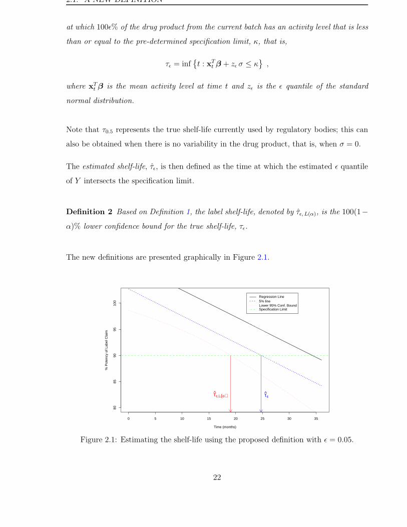
The estimated shelf-life, τε, is then defined as the time at which the estimated ε quantile
of Y intersects the specification limit.
Definition 2 Based on Definition 1, the label shelf-life, denoted by τε, L(α), is the 100(1−α)% lower confidence bound for the true shelf-life, τε.
The new definitions are presented graphically in Figure 2.1.
0 5 10 15 20 25 30 35
8085
9095
100
Time (months)
% P
oten
cy o
f Lab
el C
laim
τετε,L(α)
Regression Line5% lineLower 95% Conf. BoundSpecification Limit
Figure 2.1: Estimating the shelf-life using the proposed definition with ε = 0.05.
22

2.2. ESTIMATION OF THE LABEL SHELF-LIFE
Irrespective of the method of estimation that is used, several general points can be made
about these definitions.
1. With 100(1 − α)% confidence, at least 100(1 − ε)% of drug product will meet the
specification when the label shelf-life has been reached. Hence, the label shelf-life is
a 100(1 − α)% lower tolerance bound for the 100 ε percentile of the distribution of
shelf-lives.
2. The true shelf-life can be estimated more accurately by increasing sample size.
3. The true and label shelf-life can be extended by reducing the variability in the
manufacturing process.
Several possibilities for obtaining a label shelf-life are available. These are detailed in
the next section for linear degradation — some can easily be extended to cover multiple
regression models. Unless otherwise indicated, the terms true shelf-life, estimated shelf-life
and label shelf-life will henceforth refer to the new definitions.
2.2 Estimation of the Label Shelf-Life
Suppose the mean response is µt = xTt β = β0 + β1t, where t denotes time. Interest lies in
the ε quantile of the response, given t, which under (1.1) is given by
qt,ε = xTt β + zεσ , (2.1)
assuming that the variability does not depend on t. If there is a mean-variance relation-
ship, the methods in Chapter 4 may be more appropriate.
There are at least three possible approaches that can be used to estimate and find confi-
dence bounds for the true shelf-life as defined in Definition 1. These are based on
1. several Normal Approximation approaches,
23

2.2. ESTIMATION OF THE LABEL SHELF-LIFE
2. a variety of Profile Likelihood approaches, and
3. a Non-central t-distribution approach.
These approaches are discussed in the following sections. This work is presented in
Kiermeier et al. (2004).
2.2.1 Normal Approximation
There are various ways of estimating (2.1). Easterling (1969) suggested that the general
form of a point estimate for the shelf-life can be based on
qt,ε = β0 + β1t+ δs ,
where β0, β1 and s2 denote the least squares estimates of β0, β1 and σ2, and various
choices for δ are available. Easterling’s choice for an exact interval estimate is presented
in Section 2.2.4.
It is well known thatνs2
σ2∼ χ2
ν
where χ2ν denotes a chi-squared distribution with ν degrees of freedom (here ν = N − 2),
and thus √νs
σ∼ χν ,
where χν is a chi distribution with ν degrees of freedom. The moments of a χν variate are
given on page 421 in Johnson et al. (1994a). It can be shown that the mean and variance
of s are given by
E [ s ] = σ Cν and Var [ s ] = σ2(
1 − C2ν
)
, (2.2)
where ν = N − 2 in the linear case, and
Cν =
√
2
ν
Γ(
ν+12
)
Γ(
ν2
) ≈ 1 − 1
4ν.
24
2.2. ESTIMATION OF THE LABEL SHELF-LIFE
Since the sample mean and the sample standard deviation are independent, it follows that
E [ qt,ε ] = xTt β + δσ Cν
Var [ qt,ε ] = σ2[
xTt (XTX)−1xt + δ2
(
1 − C2ν
)]
,
and for large sample sizes qτε will be close to normally distributed with this mean and
standard deviation.
The performance of the normal approximation for qt,ε now relies on (a) the choice of δ,
and (b) the closeness to normality of s. By the Central Limit Theorem it is reasonable
to expect the distribution of qt,ε to be approximately normal for a given value of t and
choice of δ as the sample size N → ∞.
Possible choices for δ, and their resulting value, are
δ = zε (2.3)
δs is the maximum likelihood estimate for zεσ : δ = zε
√
νN, (2.4)
δs is the unbiased estimate for zεσ : δ =zε
Cν
. (2.5)
An estimate of the variance of qt,ε can be obtained by either substituting the least squares
estimate for σ, if using (2.3) or (2.5), or the maximum likelihood estimate for σ, if using
(2.4). The estimated shelf-life is given by
τε = inf t : qt,ε ≤ κ ,
and the label shelf-life is the 100(1 − α)% lower confidence bound for the time at which
qt,ε intersects the specification limit, that is,
τε,L(α) = inf
t : qτε +Qα σ√
xTt (XTX)−1xt + δ2 (1 − C2
ν ) ≤ κ
,
where σ = s for (2.3) and (2.5), and σ = s√
νN
for (2.4). Subsequent simulations will use
both zα and tα,ν as possible choices for Qα.
In the linear regression case it can be shown that τε,L(α) is the smaller positive root of t
25
2.2. ESTIMATION OF THE LABEL SHELF-LIFE
for which
β21 − Q2
ασ2
sxx
t2 + 2
β1
(
β0 − κ+ δs)
+ Q2ασ2xsxx
t
+
(β0 − κ+ δs)2 −Q2ασ
2[
1N
+ δ2(1 − C2N−2) + x2
sxx
]
= 0 , (2.6)
where sxx =∑N
i=1(xi − x)2.
2.2.2 Various Profile Likelihood Based Approaches
The label shelf-life τε,L(α) is the smallest time for which the null hypothesis
H0 : β0 + β1τε + zεσ = κ (2.7)
is not rejected on a one-sided 100α% level test. Since κ and zε are known, the likeli-
hood can be reformulated as a function of the parameters β1, σ2, τε, by substituting
β0 = κ− β1τε − zεσ. Hypotheses about τε can then be tested using the profile likelihood
for τε, denoted by
L(τε) = L(τε, β1,τε, σ2τε
;y)
where β1,τε and σ2τε
are the maximum likelihood estimates of β1,τε and σ2τε
for given values of
τε. This likelihood can be used like a genuine likelihood, and thus, the maximum likelihood
estimate of τε is equal to the overall maximum likelihood estimate τε, and confidence
intervals for τε can be constructed via the likelihood ratio test (Hinkley et al., 1991).
The Basic Profile Likelihood (PL) Approach
The log-likelihood based on (1.1) is given by
L(β, σ2;y) = −N2
log 2π − N
2log σ2 − 1
2σ2(y −Xβ)T (y −Xβ) ,
which in the linear case expands to
L(β0, β1, σ2;y) = −N
2log 2π − N
2log σ2 − 1
2σ2
N∑
i=1
(yi − β0 − β1xi)2 . (2.8)
26
2.2. ESTIMATION OF THE LABEL SHELF-LIFE
Eliminating β0 and ignoring the constant term gives the log-likelihood involving τε
L(τε, β1, σ2;y) = −N
2log σ2
τε− 1
2σ2τε
N∑
i=1
(
yi − β1,τε(xi − τε) − κ+ zεστε
)2
.
For notational simplicity, let y∗i = yi − κ and x∗i = xi − τε, giving
L(τε, β1, σ2;y) = −N
2log σ2
τε− 1
2σ2τε
N∑
i=1
(y∗i − β1,τεx∗i + zεστε)
2 . (2.9)
Differentiating with respect to β1,τε and equating to zero gives
∂L
∂β1,τε
=1
σ2τε
N∑
i=1
(y∗i − β1,τεx∗i + zεστε)x
∗i = 0 , (2.10)
which has the solution
β1,τε =Nzεστε x
∗ +∑N
i=1 x∗i y
∗i
sxx +N(x∗)2. (2.11)
Similarly, differentiating with respect to σ2τε
and setting equal to zero yields
∂L
∂σ2τε
= − N
2σ2τε
+1
2σ4τε
N∑
i=1
(y∗i −β1,τεx∗i +zεστε)
2− zε
2σ3τε
N∑
i=1
(y∗i −β1,τεx∗i +zεστε) = 0 . (2.12)
Multiplying by −2σ4τε
yields
Nσ2τε−
N∑
i=1
(y∗i − β1,τεx∗i + zεστε)
2 + zεστε
N∑
i=1
(y∗i − β1,τεx∗i + zεστε) = 0 ,
which reduces to
Nσ2τε−Nzε(y
∗ − β1,τε x∗) στε −
N∑
i=1
(y∗i − β1,τεx∗i )
2 = 0 , (2.13)
where y∗ = 1N
∑Ni=1 y
∗i = y − κ and x∗ = 1
N
∑Ni=1 x
∗i = x− τε.
Notice that the maximum likelihood estimates for β1,τε and στε rely on each other, which is
different to the unconstrained linear regression case, where β1 can generally be estimated
independently of σ. Consequently, a solution could be found by employing some iterative
scheme like Fisher scoring.
In this situation it is however possible to find an analytical solution. Write (2.11) as
β1,τε =zεx
∗
sxxVστε +
β1
NV+x∗y∗
sxxV
(2.14)
= Aστε +B ,
27
2.2. ESTIMATION OF THE LABEL SHELF-LIFE
where β1 is the usual maximum likelihood estimate of β1 that does not depend on τε,
obtained from (2.8), and
V =1
N+
(x∗)2
sxx
.
Note that (2.14) can also be written as
β1,τε = β1 +x∗
sxxV
(
y∗ − β1x∗ + zεστε
)
,
which better illustrates the modification of β1. Substituting (2.14) into (2.13) gives
Nσ2τε−Nzε
(
y∗ − [Aστε +B]x∗)
στε −N∑
i=1
(
y∗i − [Aστε +B]x∗i
)2
= 0 .
Expanding the square and collecting terms results in
Nσ2τε−Nzε(y
∗ − Bx∗) στε −N∑
i=1
(y∗i −Bx∗i )2 = 0 . (2.15)
The coefficient of στε can be rewritten as
−Nzε(y∗ − Bx∗) = −zε
V(y∗ − β1x
∗) . (2.16)
Similarly, the constant term can be expanded into
−N∑
i=1
(y∗i −Bx∗i )2 = −
N∑
i=1
(yi − y) − B(xi − x)2
− 1
NV 2
y∗ − β1x∗2
. (2.17)
The first term on the right hand side can again be expanded as follows
−N∑
i=1
(yi − y) − B(xi − x)2
= −N∑
i=1
(yi − y) − β1
NV(xi − x) − x∗y∗
sxxV(xi − x)
2
= −N∑
i=1
(yi − y) − β1
NV(xi − x)
2
− (x∗y∗)2
sxxV 2+
2 x∗y∗
sxxV
sxy −β1
NVsxx
28
2.2. ESTIMATION OF THE LABEL SHELF-LIFE
where sxy =∑N
i=1(xi − x)(yi − y) and syy =∑N
i=1(yi − y)2. Consequently,
−N∑
i=1
(yi − y) −B(xi − x)2
= − 1
N2V 2
N∑
i=1
NV (yi − y) − β1(xi − x)2
+2 (x∗)3y∗β1
sxxV 2− (x∗y∗)2
sxxV 2
= − 1
N2V 2
N∑
i=1
(yi − y) − β1(xi − x) +N(x∗)2
sxx(yi − y)
2
+2 (x∗)3y∗β1
sxxV 2− (x∗y∗)2
sxxV 2.
Note that Nσ2 =∑N
i=1
(yi − y) − β1(xi − x)2
= syy − β1sxx, where σ2 is the usual
maximum likelihood estimate of σ2 that does not depend on τε, so
−N∑
i=1
(yi − y) − B(xi − x)2
= − 1
N2V 2
Nσ2 +2N2(x∗)2σ2
sxx+N2(x∗)4syy
s2xx
+2 (x∗)3y∗β1
sxxV 2− (x∗y∗)2
sxxV 2
= − σ2
V 2
1
N+
(x∗)2
sxx
− 1
N2V 2
N2(x∗)2σ2
sxx
+N2(x∗)4(Nσ2 + β1sxy)
s2xx
+2 (x∗)3y∗β1
sxxV 2− (x∗y∗)2
sxxV 2,
which leads to
−N∑
i=1
(yi − y) −B(xi − x)2
= − σ2
V− N(x∗)2σ2
sxxV 2
1
N+
(x∗)2
sxx
− (x∗)4β21
sxxV 2+
2 (x∗)3y∗β1
sxxV 2− (x∗y∗)2
sxxV 2
= −Nσ2
V
1
N+
(x∗)2
sxx
− (x∗)2
sxxV 2
y∗ − β1x∗
= −Nσ2 − (x∗)2
sxxV 2
y∗ − β1x∗
.
Substituting back into (2.17) gives
−N∑
i=1
(y∗i − Bx∗i )2 = −Nσ2 − 1
V
y∗ − β1x∗2
,
and after using (2.16), the quadratic in σ, given in (2.15), becomes
Nσ2τε− zε
V(y∗ − β1x
∗)στε −Nσ2 − 1
V
y∗ − β1x∗2
= 0 .
29
2.2. ESTIMATION OF THE LABEL SHELF-LIFE
The estimate of στε is the positive root to this equation, given by
στε =
√
σ2 +(y∗ − β1x∗)2
4N2V 2(z2
ε + 4NV ) +zε(y
∗ − β1x∗)
2NV, (2.18)
which only depends on the maximum likelihood estimates of β1 and σ2. Consequently,
the estimate of β1,τε is found by substituting (2.18) into (2.14). Note that since zε < 0,
the last term in (2.18) shifts the estimate of στε back toward σ.
The maximum likelihood estimate of the shelf-life under this approach is given by
τε = inf
t : xTt β + zεσ ≤ κ
,
where β and σ are the maximum likelihood estimates of β and σ, respectively.
Hence, the profile likelihood for τε is
L(τε) = −N2
log σ2τε− 1
2σ2τε
N∑
i=1
(
yi − β1,τε(xi − τε) − κ+ zεστε
)2
. (2.19)
To find the label shelf-life, let L(τε) be the likelihood evaluated at the maximum likeli-
hood estimates and let L(τε) be the likelihood evaluated, for a given value of τε. Then,
asymptotically, the generalised likelihood ratio statistic is given by
w(τε) = 2(
L(τε) − L(τε))
, (2.20)
which is distributed approximately χ21. Consequently, the label shelf-life, based on the
100(1 − α)% lower confidence bound, is given by
τε,L(α) = inf
t : (t ≤ τε) &(
w(t) ≤ χ21,1−2α
)
. (2.21)
The results on likelihood ratio tests are based on large sample properties, and therefore
confidence bounds based on the likelihood ratio test may not be very accurate for small
samples. To overcome this problem, a modification to the profile likelihood has been
proposed (Barndorff-Nielsen, 1983). It will be discussed in the following section.
30
2.2. ESTIMATION OF THE LABEL SHELF-LIFE
The Modified Profile Likelihood (MPL) Approach
Consider the general likelihood problem in which scalar parameter τε needs to be esti-
mated in the presence of nuisance parameter vector (β1, σ2). A modified profile likelihood
(Barndorff-Nielsen, 1983) appropriate for estimation of τε is given by
Lm(τε) = L(τε) −1
2log∣
∣
∣I(
β1,τε , σ2τε
)
∣
∣
∣− log
∣
∣
∣
∣
∣
∂(
β1,τε, σ2τε
)
∂(
β1, σ2)
∣
∣
∣
∣
∣
, (2.22)
where I(·) denotes the observed information matrix based on L(τε) — the use of the
expected information instead of the observed is also an option (Barndorff-Nielsen, 1983).
The final term in (2.22) is the log-determinant of a matrix of derivatives, know as a
Jacobian. This Jacobian is found by differentiating (2.14) and (2.18) with respect to the
maximum likelihood estimates β1 and σ2, that is
∂(
β1,τε , σ2τε
)
∂(
β1, σ2)
=
∂β1,τε
∂β1
∂σ2τε
∂β1
∂β1,τε
∂σ2
∂σ2τε
∂σ2
From (2.10) and (2.12) it follows that the elements of the observed information matrix
are given by
Io(β1,τε , β1,τε) =sxx +N(x∗)2
σ2τε
Io(β1,τε, σ2τε
) =1
σ2τε
(
∂L
∂β1,τε
)
− Nzεx∗
2σ3τε
and
Io(σ2τε, σ2
τε) = −N(2 − z2
ε )
4σ4τε
+1
σ6τε
N∑
i=1
(y∗i − β1,τεx∗i + zεστε)
2 − 5Nzε
4σ5τε
(y∗ − β1,τεx∗ + zεστε) .
Taking expectations yields the elements of the expected information matrix
Ie(β1,τε , β1,τε) =sxx +N(x∗)2
σ2τε
Ie(β1,τε, σ2τε
) = −Nzεx∗
2σ3τε
Ie(σ2τε, σ2
τε) =
N(2 + z2ε )
4σ4τε
.
31
2.2. ESTIMATION OF THE LABEL SHELF-LIFE
The elements of the Jacobian, the last term in (2.22), are generally very difficult to obtain.
In this case however exact results are possible by differentiating (2.14) and (2.18) with
respect to the maximum likelihood estimates β1 and σ2. They are
∂σ2τε
∂σ2=
στε√
σ2 + D2(z2ε +4NV )
4N2V 2
∂σ2τε
∂β1
= −2στε
zεx∗
2NV+
D(z2ε + 4NV ) x∗
4N2V 2
√
σ2 + D2(z2ε +4NV )
4N2V 2
∂β1,τε
∂β1
=zεx
∗
2στεsxxV
(
∂σ2τε
∂β1
)
+1
NV
∂β1,τε
∂σ2=
(
∂β1,τε
∂σ2τε
)(
∂σ2τε
∂σ2
)
=zεx
∗
2στεsxxV
(
∂σ2τε
∂σ2
)
where D = y∗ − β1x∗.
The modified version of (2.20) is given by
wm(τε) = 2(
Lm(τε) − Lm(τε))
,
which is distributed approximately χ21, where τε is obtained by maximizing (2.22). Con-
sequently, the label shelf-life, based on the 100(1− α)% lower confidence bound, is given
by
τε,L(α) = inf
t : (t ≤ τε) &(
wm(t) ≤ χ21,1−2α
)
. (2.23)
In more general circumstances explicit solutions of the conditional parameters (β1,τε , σ2τε
)
in terms of the maximum likelihood parameters (β1, σ2) may not exist. Consequently, it
may not be feasible to calculate the Jacobian in those cases and the only possible solution
is to ignore this term in such instances. This will be referred to as the truncated modified
profile likelihood (TMPL).
An alternative modification to the PL, which does not require the calculation of the
Jacobian term, was presented by Cox and Reid (1987). The application of their approach
to stability testing is presented in the next section.
32
2.2. ESTIMATION OF THE LABEL SHELF-LIFE
The Approximate Conditional Profile Likelihood (ACPL) Approach
The approximate conditional profile likelihood (Cox and Reid, 1987) is
Lc(τε) = L(τε, λ) − 1
2log∣
∣
∣I(λ)
∣
∣
∣, (2.24)
where τε and λ are orthogonal parameters, and I(λ) denotes the observed information
matrix of λ, obtained from L(τε,λ), evaluated at λ — again a possible alternative is to
use of the expected information instead of the observed information. This conditional PL
is very similar to the MPL, except that the term involving the Jacobian is ignored, since
it is of order 1/N when the parameters are orthogonal. The ACPL is not invariant under
transformations of λ, but Cox & Reid have argued that the orthogonal parameterization
reduces this lack of invariance.
A set of parameters λT = (λ1, λ2), which are orthogonal to τε, can be found from the
original parameters (β1,τε , σ2τε
) by solving the differential equation (Cox and Reid, 1987,
equation (4) on page 3)
Ie(β1,τε, σ2τε
)
∂β1,τε
∂τε
∂σ2τε
∂τε
= E
∂2L∂β1,τε ∂τε
∂2L∂σ2
τε ∂τε
,
where Ie(β1,τε, σ2τε
) denotes the expected information matrix of β1,τε and σ2τε
, obtained from
(2.9). This is equivalent to solving
sxx+Nx∗
σ2τε
−Nzεx∗
2σ3τε
−Nzεx∗
2σ3τε
N(2+z2ε )
4σ4τε
∂β1,τε
∂τε
∂σ2τε
∂τε
=
Nβ1,τε x∗
σ2τε
−Nzεβ1,τε
2σ3τε
.
Consequently, the first equation is
∂β1,τε
∂τε=
2Nβ1,τε x∗
√
g(τε),
where g(τε) = sxx(2 + z2ε ) + 2N(x∗)2. Hence
∫
1
β1,τε
dβ1,τε =
∫
2Nx∗√
g(τε)dτε .
33
2.2. ESTIMATION OF THE LABEL SHELF-LIFE
Let u = 2N(x∗)2, which means that du = −4Nx∗ dτε and hence
log β1,τε = −1
2
∫
1
sxx(2 + z2ε ) + u
du
= −1
2log g(τε) + a1(λ) .
Now a1(λ) is an arbitrary function of λ. Choosing a1(λ) = log λ1 gives
λ1 = β1,τε
√
g(τε) .
The second equation is∂σ2
τε
∂τε= −2στε
zεsxxβ1,τε
g(τε),
and substituting for β1,τε and integrating yields
∫
1
2στε
dσ2τε
=
∫
−zεsxxλ1
g(τε)3/2dτε .
This reduces to
στε = − zεsxxλ1
(2N)3/2
∫
1
[c2 + (x∗)2]3/2dτε ,
where c2 = sxx(2+z2ε )
2N. Now, let x∗ = c tan θ, such that −dτ = c
cos2 θdθ, giving
στε =zεsxxλ1
(2N)3/2
∫
1/ cos2 θ
[c2 + c2 tan2 θ]3/2
dθ
=zεsxxλ1
(2N)3/2
∫
1
c2cos θ dθ
=zεsxxλ1
c2(2N)3/2[sin θ + a2(λ)]
=zελ1
(2 + z2ε )√
2N[sin θ + a2(λ)] ,
where again a2(λ) is an arbitrary function of λ. Since, x∗ = c tan θ and 1/ cos θ =√
sec2 θ =√
1 + tan2 θ it follows that
sin θ =x∗/c
√
1 + (x∗)2/c2=
x∗√
c2 + (x∗)2.
Letting a2(λ) = λ2 gives
στε =zεx
∗λ1
(2 + z2ε )√
g(τε)+
zελ1λ2
(2 + z2ε )√
2N,
34
2.2. ESTIMATION OF THE LABEL SHELF-LIFE
and re-arranging for λ2 gives
λ2 =√
2Nστε(2 + z2
ε ) − zεβ1,τεx∗
zεβ1,τε
√
g(τε).
The value of L(τε, λ) in (2.24) will be the same, irrespective of whether the parameteriza-
tion is in terms of (β1,τε , σ2τε
) or (λ1, λ2). The derivatives of L with respect to λ are found
by using the chain rule, that is,
∂L
∂λ1
=
(
∂L
∂β1,τε
)(
∂β1,τε
∂λ1
)
+
(
∂L
∂σ2τε
)(
∂σ2τε
∂λ1
)
∂L
∂λ2
=
(
∂L
∂σ2τε
)(
∂σ2τε
∂λ2
)
.
Similarly, the second derivatives are given by
∂L
∂λ1=
(
∂2L
∂β21,τε
)(
∂β1,τε
∂λ1
)2
+ 2
(
∂2L
∂β1,τε ∂σ2τε
)(
∂σ2τε
∂λ1
)(
∂β1,τε
∂λ1
)
+
(
∂2L
∂(σ2τε
)2
)(
∂σ2τε
∂λ1
)2
+
(
∂L
∂σ2τε
)(
∂2σ2τε
∂λ21
)
∂2L
∂λ2 ∂λ1=
∂2L
∂λ1 ∂λ2=
(
∂2L
∂(σ2τε
)2
)(
∂σ2τε
∂λ1
)(
∂σ2τε
∂λ2
)
+
(
∂2L
∂σ2τε∂β1,τε
)(
∂β1,τε
∂λ1
)(
∂σ2τε
∂λ2
)
+
(
∂L
∂σ2τε
)(
∂2σ2τε
∂λ1 ∂λ2
)
∂2L
∂λ22
=
(
∂2L
∂(σ2τε
)2
)(
∂σ2τε
∂λ2
)2
+
(
∂L
∂σ2τε
)(
∂2σ2τε
∂λ22
)
.
The derivatives of L with respect to β1,τε and σ2τε
are given by (2.10) and (2.12). The
derivatives of β1,τε and σ2τε
with respect to λ1 are given by
∂β1,τε
∂λ1=
1√
g(τε)
∂σ2τε
∂λ2=λ2
1z2ε
(
x∗√
2N + λ2
√
g(τε))
N(2 + z2ε )√
g(τε)
∂σ2τε
∂λ1
=λ1z
2ε
(
x∗√
2N + λ2
√
g(τε))2
N(2 + z2ε ) g(τε)
∂2σ2τε
∂λ22
=λ2
1z2ε
N(2 + z2ε )
∂2σ2τε
∂λ21
=z2
ε
(
x∗√
2N + λ2
√
g(τε))2
N(2 + z2ε ) g(τε)
∂2σ2τε
∂λ1 ∂λ2
=2λ1z
2ε
(
x∗√
2N + λ2
√
g(τε))
N(2 + z2ε )√
g(τε).
35
2.2. ESTIMATION OF THE LABEL SHELF-LIFE
The generalised likelihood ratio statistic based on the conditional PL is given by
wc(τε) = 2(
Lc(τε;y) − Lc(τε;y))
,
which is distributed approximately χ21, where τε is obtained by maximizing (2.24). Con-
sequently, the label shelf-life, based on the 100(1− α)% lower confidence bound, is given
by
τε,L(α) = inf
t : (t ≤ τε) ∩(
wc(t) ≤ χ21,1−2α
)
. (2.25)
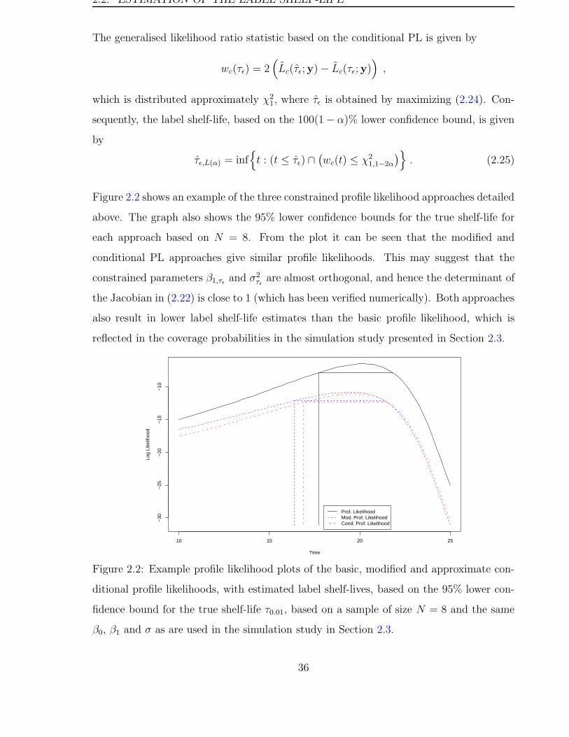
Figure 2.2 shows an example of the three constrained profile likelihood approaches detailed
above. The graph also shows the 95% lower confidence bounds for the true shelf-life for
each approach based on N = 8. From the plot it can be seen that the modified and
conditional PL approaches give similar profile likelihoods. This may suggest that the
constrained parameters β1,τε and σ2τε
are almost orthogonal, and hence the determinant of
the Jacobian in (2.22) is close to 1 (which has been verified numerically). Both approaches
also result in lower label shelf-life estimates than the basic profile likelihood, which is
reflected in the coverage probabilities in the simulation study presented in Section 2.3.
10 15 20 25
−30
−25
−20
−15
−10
Time
Log
Like
lihoo
d
Prof. LikelihoodMod. Prof. LikelihoodCond. Prof. Likelihood
Figure 2.2: Example profile likelihood plots of the basic, modified and approximate con-
ditional profile likelihoods, with estimated label shelf-lives, based on the 95% lower con-
fidence bound for the true shelf-life τ0.01, based on a sample of size N = 8 and the same
β0, β1 and σ as are used in the simulation study in Section 2.3.
36
2.2. ESTIMATION OF THE LABEL SHELF-LIFE
2.2.3 Constrained Profile Likelihood (CPL) Based Approaches
The approaches presented in Section 2.2.2 depend on the elimination of β0. This may
not be possible in a more general setting. However, as will be shown in this section, the
constrained profile likelihood provides an alternative, yet equivalent, approach.
Again, consider the general likelihood problem where the parameters θT = (β0, β1, σ2)
need to be estimated. However, the parameters are now required to satisfy (2.7) for a
given value of τε. Consequently, denote these constrained parameters by θτε and write
the constraint as
g(θτε ; τε) = β0,τε + β1,τετε + zεστε − κ = 0 . (2.26)
One way of estimating maximum likelihood parameters under a constraint is via La-
grangian multipliers, that is, by maximizing the function
L(θτε;y) − λg(θτε; τε) , (2.27)
where λ is a Lagrangian multiplier. This can be done by differentiating with respect to
θτε and λ, and employing an iterative maximization scheme. If the constraint is linear in
the parameters θτε, then the second derivative of g(θτε ; τε) with respect to θτε is zero, and
hence does not contribute to the information matrix. If, however, the constraint is not
linear in some parameters, then the second derivative will not equal zero. In particular,
this second derivative can be very complicated, making estimation more difficult.
An alternative approach is based on an augmented form of Lagrangian multipliers, referred
to as the Powell-Hestenes method (Osborne, 2000). The advantage of this alternative is
that the second derivative of the constraint is not required. Osborne suggests minimizing
an objective function which is a scaled version of the negative log-likelihood — this is
equivalent to maximizing the log-likelihood. The Powell-Hestenes method is used only
for estimation of the parameters, given a value of τε. The profile likelihood for τε is then
obtained by evaluating (2.8) at (β0,τε , β1,τε, σ2τε
).
The objective function, based on the log-likelihood (2.8) and the constraint (2.26), takes
37
2.2. ESTIMATION OF THE LABEL SHELF-LIFE
the form
H(θτε; τε,y) =1
N
[
−L(θτε)]
+ ω[
g(θτε ; τε) + ψτε
]2, (2.28)
where ω governs the importance placed on the constraint at each iteration. Generally, ω
is fixed and chosen to be of order O(√N) and ψτε is an ancillary parameter, similar to
the Lagrangian multiplier λ. Osborne (2000) shows that the update for ψτε at the m-th
iteration is given by
ψ(m+1)τε
= ψ(m)τε
+ g(
θ(m)τε
; τε)
.
The scores with respect to βτεand σ2
τεare
∂H
∂βτε
=1
N
[
− 1
σ2τε
XT (y −Xβτε)
]
+ 2ω[
g(θτε ; τε) + ψτε
]
xτε
∂H
∂σ2τε
=1
N
[
N
2σ2τε
− 1
2σ4τε
(y −Xβτε)T (y −Xβτε
)
]
+ωzε
στε
[g(θτε ; τε) + ψτε ] .
In the constrained case, the second derivatives of (2.28) with respect to the parameters
give the elements of an equivalent to the observed information matrix which is denoted
by Io′ to distinguish it from the actual information matrix, Io, which is based on the
log-likelihood (2.8),
Io′(βτε
,βτε) =
∂2H
∂βτε∂βT
τε
=1
N
[
XTX
σ2τε
]
+ 2ω xτεxTτε
Io′(βτε
, σ2τε
) =∂2H
∂βτε∂σ2
τε
=1
N
[
1
σ4τε
XT (y −Xβτε)
]
+ωzε
στε
xτε
Io′(σ2
τε, σ2
τε) =
∂2H
∂σ2τε∂σ2
τε
=1
N
[
− N
2σ4τε
+1
σ6τε
(y −Xβτε)T (y −Xβτε
)
]
+ωz2
ε
2σ2τε
.
Note that components containing the second derivative of g(θτε ; τε) have been omitted
based on the argument given by Osborne (2000).
Taking expectations gives components of a matrix which is equivalent to the expected
38

2.2. ESTIMATION OF THE LABEL SHELF-LIFE
information matrix, denoted by Ie′. They are given by
Ie′(βτε
,βτε) =
1
N
[
XTX
σ2τε
]
+ 2ω xτεxTτε
Ie′(βτε
, σ2τε
) = 0 +ωzε
στε
xτε
Ie′(σ2
τε, σ2
τε) =
1
N
[
N
2σ4τε
]
+ωz2
ε
2σ2τε
.
Note that the relationship between Io′ and Io is
Io′ =
1
NIo + 2ωCτεC
Tτε,
where Cτε is the p× 1 vector of derivatives of the constraint such that
Cτε =∂g(θτε ; τε)
∂θτε
.
The same relationship also holds for Ie′ and Ie.
Estimates for βτεand σ2
τεcan then be found using Fisher scoring. These estimates can
be substituted into the likelihood and the likelihood can be profiled over τε, resulting in
L(τε; β0,τε, β1,τε , σ2τε,y) = −N
2log 2π − N
2log σ2
τε− 1
2σ2τε
N∑
i=1
(yi − β0,τε − β1,τεxi)2 . (2.29)
The maximum likelihood estimate of τε is the value which minimises this profile likelihood.
The unconstrained parameter estimates of β and σ2 can be found by setting ω = 0 and
solving for θ = (β, σ2).
The constrained version of (2.20) is given by
w(τε) = 2(
L(βτε, σ2
τε; τε,y) − L(βτε
, σ2τε
; τε,y))
,
which is distributed approximately χ21, where the estimates of βτε
and σ2τε
are obtained
by maximizing (2.28), and the estimate of τε is obtained by solving g(θ ; τε) = 0 for τε.
Consequently, the label shelf-life, based on the 100(1 − α)% lower confidence bound, is
given by
τε,L(α) = inf
t : (t ≤ τε) &(
w(t) ≤ χ21,1−2α
)
. (2.30)
39
2.2. ESTIMATION OF THE LABEL SHELF-LIFE
The label shelf-life obtained using this method should be identical to that obtained using
the basic profile likelihood in Section 2.2.2. This has been verified numerically.
Comments made about the large sample properties of the profile likelihood also apply here.
Consequently, a modification to the CPL, similar to that suggested by Barndorff-Nielsen
(1983), is desirable. Such a modification is developed below.
The Truncated Modified Constrained Profile Likelihood (TMCPL) Approach
The previous section showed that the constrained parameters cannot be expressed ex-
plicitly in terms of the unconstrained maximum likelihood estimates. Consequently, a
Jacobian term analogous to the one used in (2.22) cannot be obtained. One option is to
ignore the Jacobian term (Barndorff-Nielsen, 1983) and adjust the profile likelihood (2.29)
purely with the log determinant of the appropriate information matrix. This approach
is adopted here and the resulting method shall be termed truncated modified constrained
profile likelihood (TMCPL) to distinguish it from the previously mentioned truncated
modified profile likelihood.
To adjust the profile likelihood under the general constrained estimation approach pre-
sented in Section 2.2.3 the appropriate information matrix is required. The observed
information matrix Io(θτε) based on (2.29) can easily be calculated and evaluated at the
parameter estimates θτε. However due to the constraint the parameters are linearly de-
pendent. This means that Io(θτε) is not of full column rank, and has a zero determinant.
Consequently, the adjustment which is based on the log determinant cannot be made.
However, the approach suggested below approximates the “correct” information matrix
used in (2.22).
This can be done by recognizing that the basic profile likelihood (2.19) and the constrained
profile likelihood (2.29) must be the same for any given value of τε. In addition, since
g(θτε ; τε) = 0, the equality can be written as
L(τε ; ϑτε) = L(τε ; θτε) + λg(θτε ; τε) , (2.31)
40
2.2. ESTIMATION OF THE LABEL SHELF-LIFE
where ϑTτε
= (β1,τε, σ2τε
) denote the parameters under the basic profile likelihood model,
θTτε
= (β0,τε, β1,τε, σ2τε
) denote the parameters under the constrained profile likelihood
model, λ is a Lagrangian multiplier, and the last term on the right hand side is zero
when the constraint is satisfied.
The constraint g(θτε ; τε) can be approximated using a Taylor Series expansion about
θτε = θ0,τε , say, that is,
g(θτε ; τε) ≈ g(θ0,τε ; τε) +∂ g(θτε ; τε)
∂θTτε
∣
∣
∣
∣
∣
θτε=θ0,τε
(θτε − θ0,τε) .
Since both θτε and θ0,τε must satisfy the constraint, it follows that
0 ≈ 0 + C0(θτε − θ0,τε) ,
where C0 is the 1×p matrix of derivatives evaluated at θ0,τε. Hence, let C0θ0,τε = c0, say.
Substituting into (2.31) gives
L(τε ; ϑτε) ≈ L(τε ; θτε) + λ[
C0θτε − c0
]
. (2.32)
Let L0 be the orthonormal matrix of size (p− 1) × p, orthogonal to C0, that is,
C0LT0 = 0 and L0L
T0 = Ip−1 ,
and write
T0θτε =
L0
C0
θτε =
ϑτε
c0
. (2.33)
Differentiating (2.32) with respect to ϑj,τε gives
∂L(τε,ϑτε)
∂ϑj,τε
≈ ∂L(θτε)
∂θTτε
∂θτε
∂ϑj,τε
+ λC0∂θτε
∂ϑj,τε
,
and differentiating again with respect to ϑk,τε gives
∂2L(ϑτε)
∂ϑj,τε ∂ϑk,τε
≈(
∂θTτε
∂ϑk,τε
)(
∂2L(θτε)
∂θτε ∂θTτε
)(
∂θτε
∂ϑj,τε
)
+
(
∂L(θτε)
∂θTτε
)(
∂2θτε
∂ϑj,τε ∂ϑk,τε
)
+ λC0∂2θτε
∂ϑj,τε ∂ϑk,τε
.
41

2.2. ESTIMATION OF THE LABEL SHELF-LIFE
From (2.33) it follows that
T0∂θτε
∂ϑj,τε
= ej ,
where ej is a vector of zeros, except for a 1 in the j-th position. Now, differentiating
again gives
T0∂2θτε
∂ϑj,τε ∂ϑk,τε
= 0 ,
which, since T0 is of full column rank, means that ∂2θτε
∂ϑj,τε ∂ϑk,τε= 0. Hence
∂2L(ϑτε)
∂ϑj,τε ∂ϑk,τε
≈(
∂θTτε
∂ϑk,τε
)(
∂2L(θτε)
∂θτε ∂θTτε
)(
∂θτε
∂ϑj,τε
)
Since ∂θτε
∂ϑj,τε= T−1
0 ej it follows that
∂2L(ϑτε)
∂ϑj,τε ∂ϑk,τε
≈ eTj T
−T0
(
∂2L(θτε)
∂θτε ∂θTτε
)
T−10 ej ,
where T−T0 =
(
T−10
)T. Consequently, the equivalent to the observed information matrix
of ϑτε is given by
Io′(ϑτε) ≈
[
T−T0 Io(θτε)T
−10
]
(Upper left p − 1 matrix)
.
The inverse of T0 is given by
T−10 =
[
LT0
(
L0LT0
)−1CT
0
(
C0CT0
)−1]
=[
LT0 CT
0
(
C0CT0
)−1]
,
such that
T−T0 Io(θτε)T
−10 =
L0Io(θτε)LT0 L0Io(θτε)C
T0
(
C0CT0
)−1
(
C0CT0
)−1C0Io(θτε)L
T0
(
C0CT0
)−1C0Io(θτε)C
T0
(
C0CT0
)−1
,
Consequently,
Io′(ϑτε) ≈ L0Io(θτε)L
T0 , (2.34)
where Io′(ϑτε) is the appropriate equivalent to the information matrix for use in the
modified profile likelihood.
On the other hand,
det
T−T0 Io(θτε)T
−10
=[
det
T0TT0
]−1
det
Io(θτε)
=[
det
C0CT0
]−1
det
Io(θτε)
, (2.35)
42
2.2. ESTIMATION OF THE LABEL SHELF-LIFE
since
det
T0TT0
= det
L0LT0 0
0 C0CT0
= det
C0CT0
.
But also
det
T−T0 Io(θτε)T
−10
= det
L0Io(θτε)LT0
det
(
C0CT0
)−1C0Io(θτε)C
T0
(
C0CT0
)−1
−(
C0CT0
)−1C0Io(θτε)L
T0
(
L0Io(θτε)LT0
)−1L0Io(θτε)C
T0
(
C0CT0
)−1
.
The second determinant on the right hand side can now be written as
det
(
C0CT0
)−1C0
[
Io(θτε) − Io(θτε)LT0
(
L0Io(θτε)LT0
)−1L0Io(θτε)
]
CT0
(
C0CT0
)−1
= det
(
C0CT0
)−1C0C
T0
(
C0Io(θτε)−1CT
0
)−1C0C
T0
(
C0CT0
)−1
=[
det
C0Io(θτε)−1CT
0
]−1
.
Consequently,
det
T−T0 Io(θτε)T
−10
= det
L0Io(θτε)LT0
[
det
C0Io(θτε)−1CT
0
]−1
. (2.36)
Combining (2.35) and (2.36) gives
det
L0Io(θτε)LT0
= det
C0Io(θτε)−1CT
0
[
det
C0CT0
]−1
det
Io(θτε)
. (2.37)
This means that, as long as C0 is known, there is no need to know the form of L0.
The form of C0 can be obtained by differentiating (2.26), that is,
∂g(θτε, τε)
∂θTτε
=[
1 τεzε
2στε
]
θτε= θ0,τε
.
An obvious choice for θ0,τε is the constrained maximum likelihood estimate θτε , such that
C0 =[
1 τεzε
2στε
]
.
The approximate modified profile likelihood is now given by
Lt(τε;y) = L(θτε ;y) − 1
2log
[
det
C0Io(θτε)−1CT
0
[
det
C0CT0
]−1
det
Io(θτε)
]
43

2.2. ESTIMATION OF THE LABEL SHELF-LIFE
from which τε can be estimated.
The generalised likelihood ratio statistic is given by
wt(τε) = 2(
Lt(τε;y) − Lt(τε;y))
,
which is distributed approximately χ21. Consequently, the label shelf-life, based on the
100(1 − α)% lower confidence bound, is given by
τε,L(α) = inf
t : (t ≤ τε) & (wt(t) ≤ χ21,1−2α)
. (2.38)
Again, the expected information matrix can be used instead of the observed information
matrix.
However, it does not matter which information matrix is used, as both give the same
adjustment to the likelihood. This is the case if it can be shown that the observed
information matrix can be expressed in a form that does not involve the data. To do
this, first consider the score vector for the constrained problem which equals zero at the
constrained maximum likelihood estimate. Hence it follows that the elements of the score
can be written as
1
σ2τε
XT (y −Xβτε) = 2Nω
[
g(θτε ; τε) + ψτε
]
xτε
and1
2σ4τε
(y −Xβτε)T (y −Xβτε
) =N
2σ2τε
+Nωzε
στε
[
g(θτε ; τε) + ψτε
]
.
The left hand sides of these two equations now also feature in the equivalents of the
observed information matrix elements Io′(βτε
, σ2τε
) and Io′(σ2
τε, σ2
τε). Hence these elements
can be written at the constrained maximum likelihood estimates as
Io′(βτε
, σ2τε
) =2ω
σ2τε
[
g(θτε ; τε) + ψτε
]
xτε +ωzε
στε
xτε
Io′(σ2
τε, σ2
τε) =
N
2σ4τε
+2Nzεω
σ3τε
[
g(θτε ; τε) + ψτε
]
.
This now proves that the Powell-Hestenes equivalent of the observed information matrix
can be expressed in terms that do not involve the data. Thus, taking expectations will
have no effect on the adjustment term.
44
2.2. ESTIMATION OF THE LABEL SHELF-LIFE
2.2.4 Non-central t-distribution (NCT) Approach
As pointed out in Section 2.1, this approach was suggested by Easterling (1969). The
exact approach given here serves as a gold standard against which the other methods
given in this chapter can be compared. However, it is shown in Chapter 3 that this
approach cannot generally be used in the case when multiple batches are used in the
estimation of the label shelf-life. Thus it is specifically for the single batch case, and for
multiple batches another approach is necessary.
The distribution of the least squares estimate of β is given by
β ∼ N
β, σ2(XTX)−1
.
Consequently, the distribution of the estimated mean response at time t, µt = xTt β, is
µt ∼ N
µt, σ2xT
t (XTX)−1xt
Standardizing µt and using (2.1) to replace the mean µt by qτ,ε − zεσ, gives
µt − qτ,ε + zεσ
σ√
xTt (XTX)−1xt
∼ N(0, 1) ,
or equivalently,
µt − qτ,ε
σ√
xTt (XTX)−1xt
∼ N
−zε√
xTt (XTX)−1xt
, 1
.
Since the mean of this distribution does not involve σ, replacing σ by s results in
µt − qτ,ε
s√
xTt (XTX)−1xt
∼ t′N−2(δ) ,
where t′N−2(δ) denotes a non-central t-distribution with N − 2 degrees of freedom and
non-centrality parameter δ = −zε/√
xTt (XTX)−1xt.
An estimate of the shelf-life is given by
τε = inf t : µt + zεs ≤ κ ,
and the label shelf-life is given by the intersection of the exact 100(1−α)% lower confidence
bound and the specification limit, that is,
τε,L(α) = inf
t : µt +Qαs√
xTt (XTX)−1xt ≤ κ
.
45
2.3. SIMULATION RESULTS
where Qα = t′α,N−2(−δ), the α quantile of the t′N−2(−δ) distribution, which equals
−t′1−α,N−2(δ). In the linear regression case, the label shelf-life τε,L(α) is the positive root
of
β21 −
Q2αs
2
sxx
t2 + 2
β1(β0 − κ) +Q2
αs2x
sxx
t+
(β0 − κ)2 −Q2αs
2
[
1
N+x2
sxx
]
= 0 .
(2.39)
2.3 Simulation Results
Since real pharmaceutical stability data is generally commercially sensitive, the approaches
detailed in Section 2.2 have been evaluated with the help of a simulation study using the
software package R (Ihaka and Gentleman, 1996).
The simulations were conducted as follows. A random sample of size r was drawn at each
of n times xi = 0, 3, 6, 9, 12, 18, 24, and 36 months from N(xTi β, σ2), where xT
i = (1, xi)
and βT = (100, β1). This can be done without loss of generality as the approaches,
except the approximate conditional profile likelihood approach, are invariant under linear
transformations. The total number of observations available for analysis is N = nr = 8r.
Values of β1 = −0.2, -0.3 and -0.4, σ = 0.5, 1 and 2, and r = 1, 2, 5, 10, 20, and 50
were used. For each combination of β1, σ and r, 1000 simulations were performed and the
proportion of label shelf-lives less than the true shelf-life was determined for each method.
The true mean degradation lines for each β1 are shown in Figure 2.3.
Assuming that κ = 90 and ε = 0.01, the true shelf-life (in months) is given by τ0.01 =
(90 − β0 − z0.01σ)/β1. The true shelf-lives for each parameter combination of β1 and σ
are given in Table 2.1. For each simulation the label shelf-life τ0.01,L(0.05), based on a
significance level of α = 0.05, was calculated.
For each approach the proportion of label shelf-lives that were less than the true shelf-life
is tabled in Tables 2.2–2.10. In addition, the bias and the Mean Square Error (MSE) were
calculated and tabulated in Tables 2.11–2.19 and Tables 2.20–2.28, respectively.
46
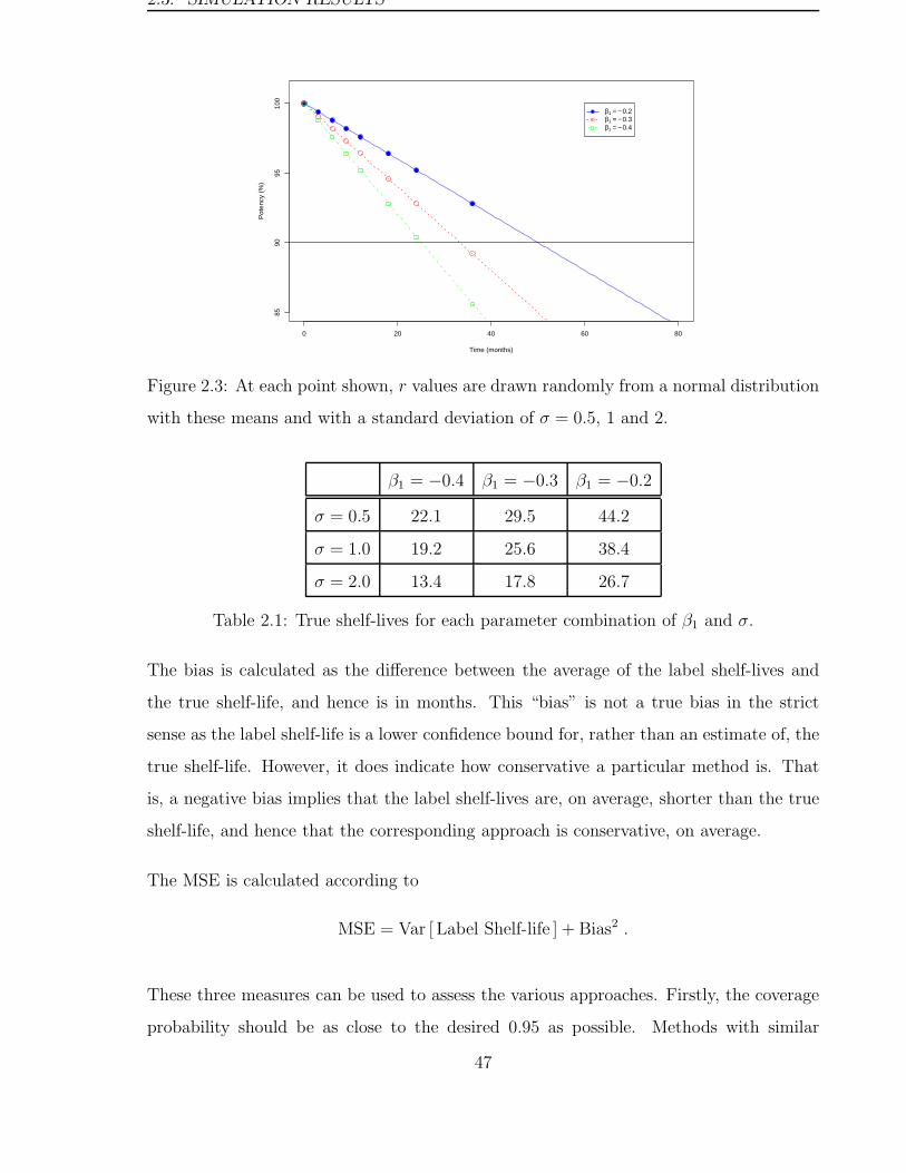
2.3. SIMULATION RESULTS
0 20 40 60 80
8590
9510
0
Time (months)
Pot
ency
(%
)
β1 = − 0.2β1 = − 0.3β1 = − 0.4
Figure 2.3: At each point shown, r values are drawn randomly from a normal distribution
with these means and with a standard deviation of σ = 0.5, 1 and 2.
β1 = −0.4 β1 = −0.3 β1 = −0.2
σ = 0.5 22.1 29.5 44.2
σ = 1.0 19.2 25.6 38.4
σ = 2.0 13.4 17.8 26.7
Table 2.1: True shelf-lives for each parameter combination of β1 and σ.
The bias is calculated as the difference between the average of the label shelf-lives and
the true shelf-life, and hence is in months. This “bias” is not a true bias in the strict
sense as the label shelf-life is a lower confidence bound for, rather than an estimate of, the
true shelf-life. However, it does indicate how conservative a particular method is. That
is, a negative bias implies that the label shelf-lives are, on average, shorter than the true
shelf-life, and hence that the corresponding approach is conservative, on average.
The MSE is calculated according to
MSE = Var [ Label Shelf-life ] + Bias2 .
These three measures can be used to assess the various approaches. Firstly, the coverage
probability should be as close to the desired 0.95 as possible. Methods with similar
47
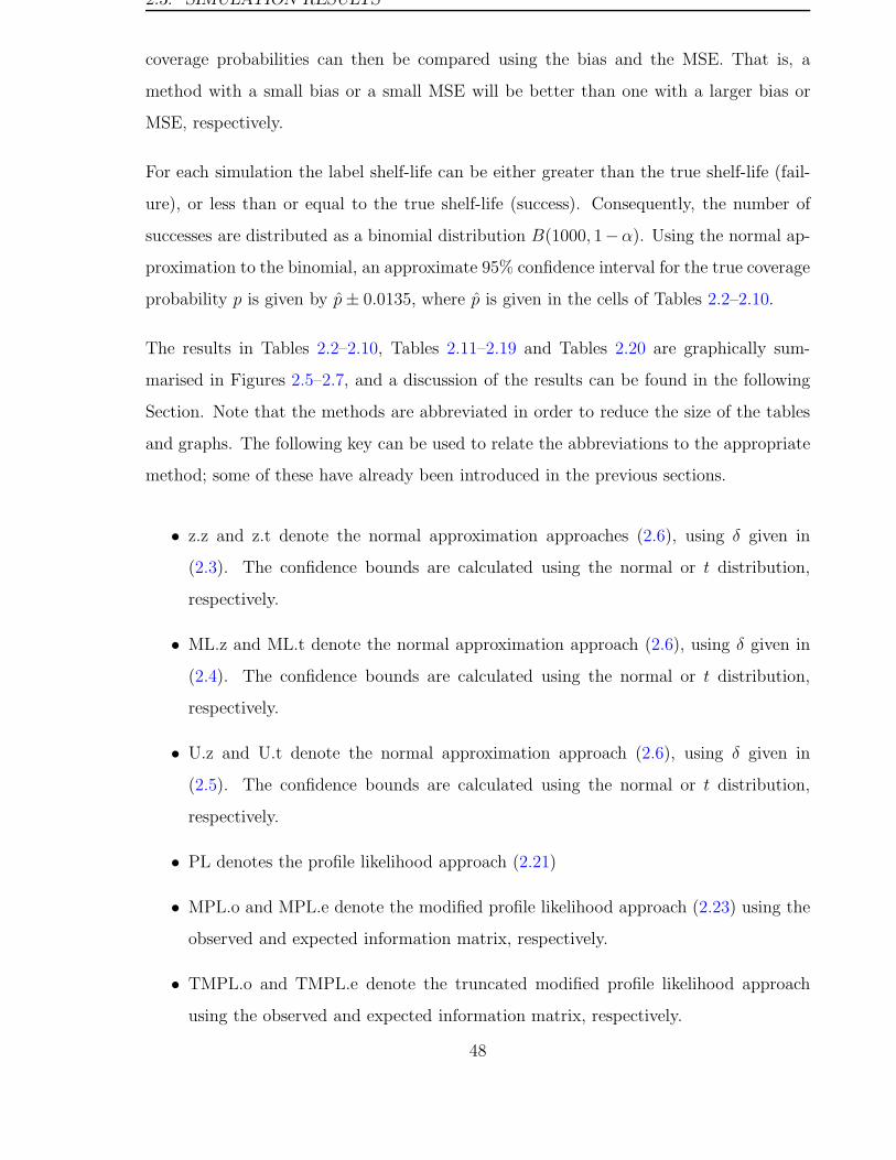
2.3. SIMULATION RESULTS
coverage probabilities can then be compared using the bias and the MSE. That is, a
method with a small bias or a small MSE will be better than one with a larger bias or
MSE, respectively.
For each simulation the label shelf-life can be either greater than the true shelf-life (fail-
ure), or less than or equal to the true shelf-life (success). Consequently, the number of
successes are distributed as a binomial distribution B(1000, 1−α). Using the normal ap-
proximation to the binomial, an approximate 95% confidence interval for the true coverage
probability p is given by p± 0.0135, where p is given in the cells of Tables 2.2–2.10.
The results in Tables 2.2–2.10, Tables 2.11–2.19 and Tables 2.20 are graphically sum-
marised in Figures 2.5–2.7, and a discussion of the results can be found in the following
Section. Note that the methods are abbreviated in order to reduce the size of the tables
and graphs. The following key can be used to relate the abbreviations to the appropriate
method; some of these have already been introduced in the previous sections.
• z.z and z.t denote the normal approximation approaches (2.6), using δ given in
(2.3). The confidence bounds are calculated using the normal or t distribution,
respectively.
• ML.z and ML.t denote the normal approximation approach (2.6), using δ given in
(2.4). The confidence bounds are calculated using the normal or t distribution,
respectively.
• U.z and U.t denote the normal approximation approach (2.6), using δ given in
(2.5). The confidence bounds are calculated using the normal or t distribution,
respectively.
• PL denotes the profile likelihood approach (2.21)
• MPL.o and MPL.e denote the modified profile likelihood approach (2.23) using the
observed and expected information matrix, respectively.
• TMPL.o and TMPL.e denote the truncated modified profile likelihood approach
using the observed and expected information matrix, respectively.
48
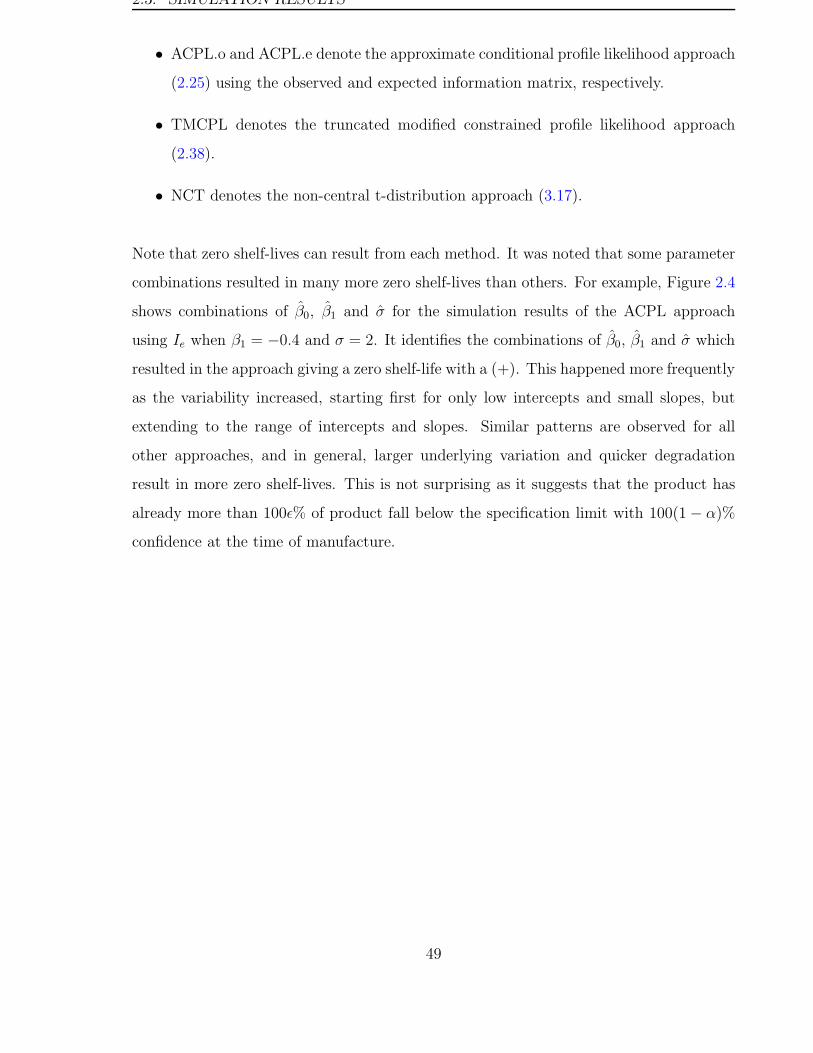
2.3. SIMULATION RESULTS
• ACPL.o and ACPL.e denote the approximate conditional profile likelihood approach
(2.25) using the observed and expected information matrix, respectively.
• TMCPL denotes the truncated modified constrained profile likelihood approach
(2.38).
• NCT denotes the non-central t-distribution approach (3.17).
Note that zero shelf-lives can result from each method. It was noted that some parameter
combinations resulted in many more zero shelf-lives than others. For example, Figure 2.4
shows combinations of β0, β1 and σ for the simulation results of the ACPL approach
using Ie when β1 = −0.4 and σ = 2. It identifies the combinations of β0, β1 and σ which
resulted in the approach giving a zero shelf-life with a (+). This happened more frequently
as the variability increased, starting first for only low intercepts and small slopes, but
extending to the range of intercepts and slopes. Similar patterns are observed for all
other approaches, and in general, larger underlying variation and quicker degradation
result in more zero shelf-lives. This is not surprising as it suggests that the product has
already more than 100ε% of product fall below the specification limit with 100(1 − α)%
confidence at the time of manufacture.
49
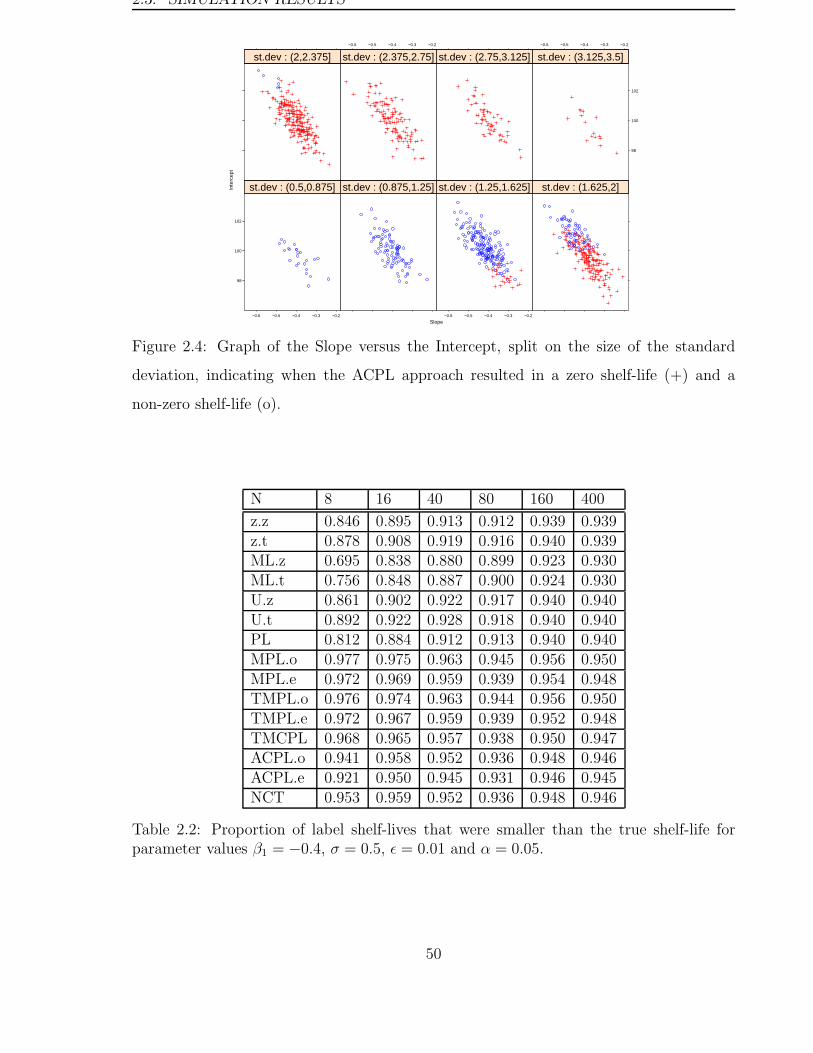
2.3. SIMULATION RESULTS
Slope
Inte
rcep
t
98
100
102
−0.6 −0.5 −0.4 −0.3 −0.2
st.dev : (0.5,0.875] st.dev : (0.875,1.25]
−0.6 −0.5 −0.4 −0.3 −0.2
st.dev : (1.25,1.625] st.dev : (1.625,2]
st.dev : (2,2.375] st.dev : (2.375,2.75]−0.6 −0.5 −0.4 −0.3 −0.2
st.dev : (2.75,3.125]
98
100
102
st.dev : (3.125,3.5]−0.6 −0.5 −0.4 −0.3 −0.2
Figure 2.4: Graph of the Slope versus the Intercept, split on the size of the standard
deviation, indicating when the ACPL approach resulted in a zero shelf-life (+) and a
non-zero shelf-life (o).
N 8 16 40 80 160 400
z.z 0.846 0.895 0.913 0.912 0.939 0.939z.t 0.878 0.908 0.919 0.916 0.940 0.939ML.z 0.695 0.838 0.880 0.899 0.923 0.930ML.t 0.756 0.848 0.887 0.900 0.924 0.930U.z 0.861 0.902 0.922 0.917 0.940 0.940U.t 0.892 0.922 0.928 0.918 0.940 0.940PL 0.812 0.884 0.912 0.913 0.940 0.940MPL.o 0.977 0.975 0.963 0.945 0.956 0.950MPL.e 0.972 0.969 0.959 0.939 0.954 0.948TMPL.o 0.976 0.974 0.963 0.944 0.956 0.950TMPL.e 0.972 0.967 0.959 0.939 0.952 0.948TMCPL 0.968 0.965 0.957 0.938 0.950 0.947ACPL.o 0.941 0.958 0.952 0.936 0.948 0.946ACPL.e 0.921 0.950 0.945 0.931 0.946 0.945NCT 0.953 0.959 0.952 0.936 0.948 0.946
Table 2.2: Proportion of label shelf-lives that were smaller than the true shelf-life forparameter values β1 = −0.4, σ = 0.5, ε = 0.01 and α = 0.05.
50
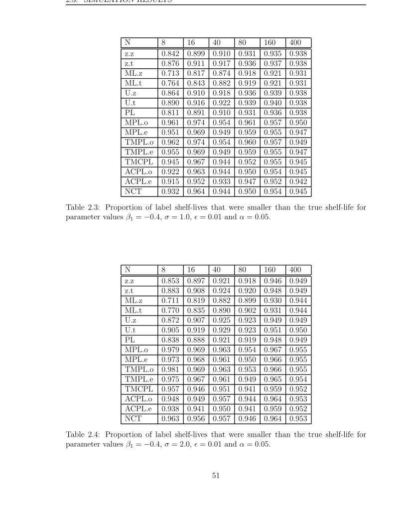
2.3. SIMULATION RESULTS
N 8 16 40 80 160 400
z.z 0.842 0.899 0.910 0.931 0.935 0.938z.t 0.876 0.911 0.917 0.936 0.937 0.938ML.z 0.713 0.817 0.874 0.918 0.921 0.931ML.t 0.764 0.843 0.882 0.919 0.921 0.931U.z 0.864 0.910 0.918 0.936 0.939 0.938U.t 0.890 0.916 0.922 0.939 0.940 0.938PL 0.811 0.891 0.910 0.931 0.936 0.938MPL.o 0.961 0.974 0.954 0.961 0.957 0.950MPL.e 0.951 0.969 0.949 0.959 0.955 0.947TMPL.o 0.962 0.974 0.954 0.960 0.957 0.949TMPL.e 0.955 0.969 0.949 0.959 0.955 0.947TMCPL 0.945 0.967 0.944 0.952 0.955 0.945ACPL.o 0.922 0.963 0.944 0.950 0.954 0.945ACPL.e 0.915 0.952 0.933 0.947 0.952 0.942NCT 0.932 0.964 0.944 0.950 0.954 0.945
Table 2.3: Proportion of label shelf-lives that were smaller than the true shelf-life forparameter values β1 = −0.4, σ = 1.0, ε = 0.01 and α = 0.05.
N 8 16 40 80 160 400
z.z 0.853 0.897 0.921 0.918 0.946 0.949z.t 0.883 0.908 0.924 0.920 0.948 0.949ML.z 0.711 0.819 0.882 0.899 0.930 0.944ML.t 0.770 0.835 0.890 0.902 0.931 0.944U.z 0.872 0.907 0.925 0.923 0.949 0.949U.t 0.905 0.919 0.929 0.923 0.951 0.950PL 0.838 0.888 0.921 0.919 0.948 0.949MPL.o 0.979 0.969 0.963 0.954 0.967 0.955MPL.e 0.973 0.968 0.961 0.950 0.966 0.955TMPL.o 0.981 0.969 0.963 0.953 0.966 0.955TMPL.e 0.975 0.967 0.961 0.949 0.965 0.954TMCPL 0.957 0.946 0.951 0.941 0.959 0.952ACPL.o 0.948 0.949 0.957 0.944 0.964 0.953ACPL.e 0.938 0.941 0.950 0.941 0.959 0.952NCT 0.963 0.956 0.957 0.946 0.964 0.953
Table 2.4: Proportion of label shelf-lives that were smaller than the true shelf-life forparameter values β1 = −0.4, σ = 2.0, ε = 0.01 and α = 0.05.
51
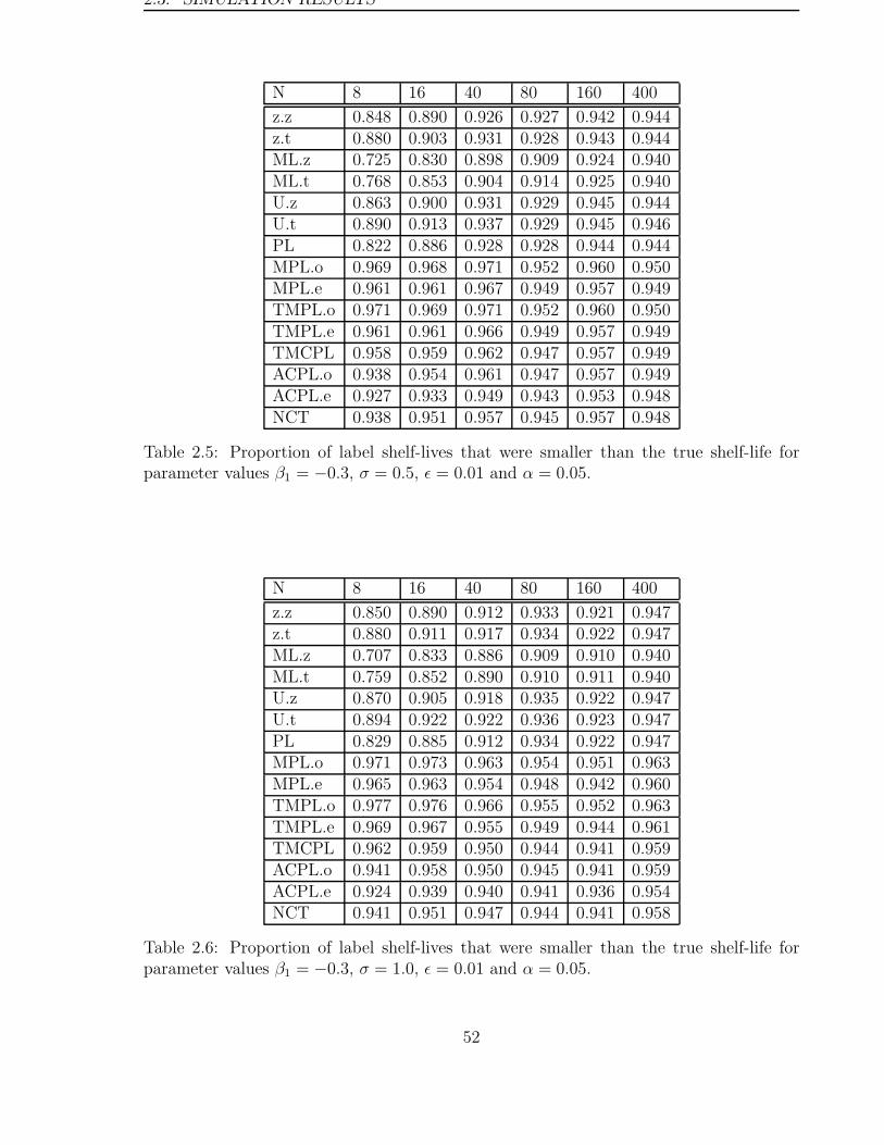
2.3. SIMULATION RESULTS
N 8 16 40 80 160 400
z.z 0.848 0.890 0.926 0.927 0.942 0.944z.t 0.880 0.903 0.931 0.928 0.943 0.944ML.z 0.725 0.830 0.898 0.909 0.924 0.940ML.t 0.768 0.853 0.904 0.914 0.925 0.940U.z 0.863 0.900 0.931 0.929 0.945 0.944U.t 0.890 0.913 0.937 0.929 0.945 0.946PL 0.822 0.886 0.928 0.928 0.944 0.944MPL.o 0.969 0.968 0.971 0.952 0.960 0.950MPL.e 0.961 0.961 0.967 0.949 0.957 0.949TMPL.o 0.971 0.969 0.971 0.952 0.960 0.950TMPL.e 0.961 0.961 0.966 0.949 0.957 0.949TMCPL 0.958 0.959 0.962 0.947 0.957 0.949ACPL.o 0.938 0.954 0.961 0.947 0.957 0.949ACPL.e 0.927 0.933 0.949 0.943 0.953 0.948NCT 0.938 0.951 0.957 0.945 0.957 0.948
Table 2.5: Proportion of label shelf-lives that were smaller than the true shelf-life forparameter values β1 = −0.3, σ = 0.5, ε = 0.01 and α = 0.05.
N 8 16 40 80 160 400
z.z 0.850 0.890 0.912 0.933 0.921 0.947z.t 0.880 0.911 0.917 0.934 0.922 0.947ML.z 0.707 0.833 0.886 0.909 0.910 0.940ML.t 0.759 0.852 0.890 0.910 0.911 0.940U.z 0.870 0.905 0.918 0.935 0.922 0.947U.t 0.894 0.922 0.922 0.936 0.923 0.947PL 0.829 0.885 0.912 0.934 0.922 0.947MPL.o 0.971 0.973 0.963 0.954 0.951 0.963MPL.e 0.965 0.963 0.954 0.948 0.942 0.960TMPL.o 0.977 0.976 0.966 0.955 0.952 0.963TMPL.e 0.969 0.967 0.955 0.949 0.944 0.961TMCPL 0.962 0.959 0.950 0.944 0.941 0.959ACPL.o 0.941 0.958 0.950 0.945 0.941 0.959ACPL.e 0.924 0.939 0.940 0.941 0.936 0.954NCT 0.941 0.951 0.947 0.944 0.941 0.958
Table 2.6: Proportion of label shelf-lives that were smaller than the true shelf-life forparameter values β1 = −0.3, σ = 1.0, ε = 0.01 and α = 0.05.
52

2.3. SIMULATION RESULTS
N 8 16 40 80 160 400
z.z 0.853 0.885 0.910 0.928 0.924 0.959z.t 0.880 0.892 0.913 0.930 0.926 0.959ML.z 0.719 0.798 0.873 0.906 0.906 0.950ML.t 0.773 0.819 0.881 0.911 0.907 0.951U.z 0.873 0.889 0.915 0.931 0.927 0.961U.t 0.902 0.908 0.920 0.933 0.930 0.961PL 0.827 0.877 0.910 0.928 0.926 0.959MPL.o 0.967 0.958 0.956 0.959 0.948 0.965MPL.e 0.963 0.953 0.951 0.953 0.945 0.964TMPL.o 0.976 0.961 0.962 0.959 0.950 0.965TMPL.e 0.972 0.958 0.954 0.954 0.946 0.965TMCPL 0.958 0.941 0.941 0.945 0.937 0.963ACPL.o 0.950 0.943 0.943 0.949 0.939 0.963ACPL.e 0.945 0.938 0.940 0.944 0.937 0.963NCT 0.957 0.943 0.943 0.949 0.939 0.963
Table 2.7: Proportion of label shelf-lives that were smaller than the true shelf-life forparameter values β1 = −0.3, σ = 2.0, ε = 0.01 and α = 0.05.
N 8 16 40 80 160 400
z.z 0.877 0.901 0.922 0.941 0.938 0.951z.t 0.909 0.917 0.929 0.944 0.938 0.952ML.z 0.786 0.862 0.903 0.929 0.933 0.946ML.t 0.839 0.877 0.907 0.932 0.934 0.946U.z 0.891 0.909 0.925 0.944 0.941 0.952U.t 0.920 0.923 0.932 0.945 0.943 0.953PL 0.859 0.897 0.922 0.943 0.938 0.952MPL.o 0.976 0.972 0.955 0.963 0.958 0.961MPL.e 0.965 0.956 0.950 0.959 0.953 0.959TMPL.o 0.980 0.975 0.957 0.963 0.959 0.961TMPL.e 0.971 0.959 0.951 0.960 0.954 0.959TMCPL 0.967 0.955 0.948 0.958 0.953 0.959ACPL.o 0.958 0.954 0.950 0.959 0.953 0.959ACPL.e 0.936 0.939 0.940 0.951 0.947 0.959NCT 0.951 0.950 0.941 0.955 0.951 0.959
Table 2.8: Proportion of label shelf-lives that were smaller than the true shelf-life forparameter values β1 = −0.2, σ = 0.5, ε = 0.01 and α = 0.05.
53
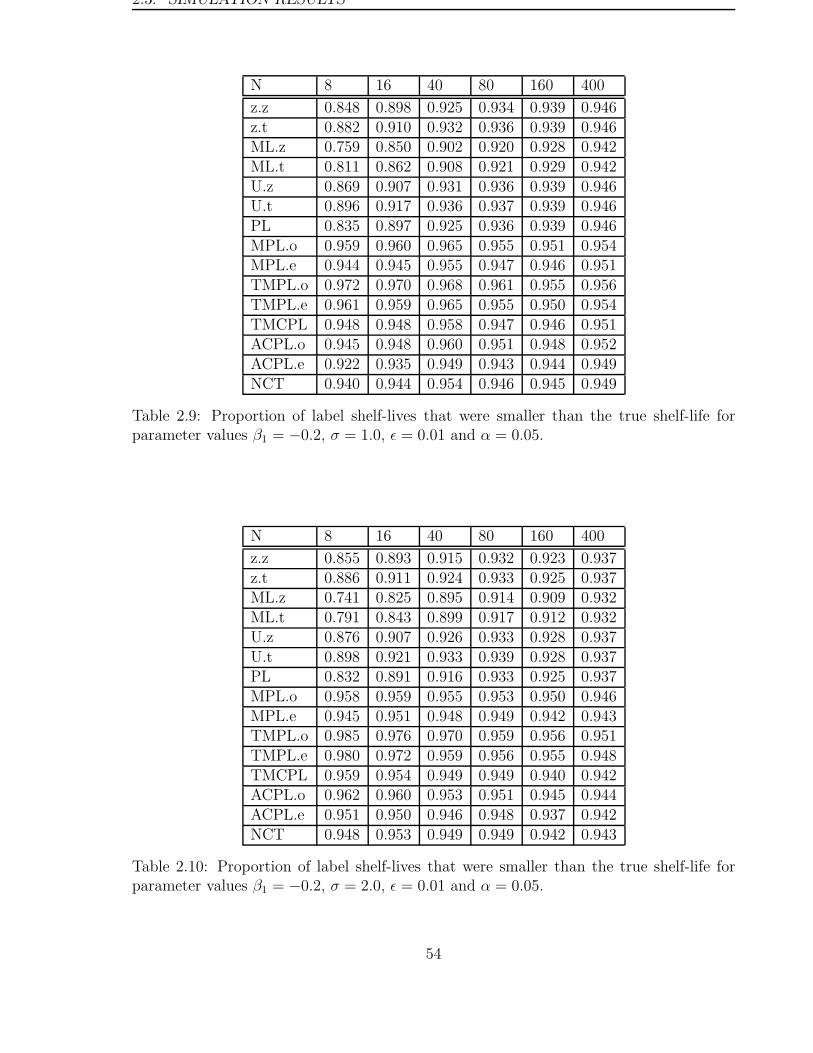
2.3. SIMULATION RESULTS
N 8 16 40 80 160 400
z.z 0.848 0.898 0.925 0.934 0.939 0.946z.t 0.882 0.910 0.932 0.936 0.939 0.946ML.z 0.759 0.850 0.902 0.920 0.928 0.942ML.t 0.811 0.862 0.908 0.921 0.929 0.942U.z 0.869 0.907 0.931 0.936 0.939 0.946U.t 0.896 0.917 0.936 0.937 0.939 0.946PL 0.835 0.897 0.925 0.936 0.939 0.946MPL.o 0.959 0.960 0.965 0.955 0.951 0.954MPL.e 0.944 0.945 0.955 0.947 0.946 0.951TMPL.o 0.972 0.970 0.968 0.961 0.955 0.956TMPL.e 0.961 0.959 0.965 0.955 0.950 0.954TMCPL 0.948 0.948 0.958 0.947 0.946 0.951ACPL.o 0.945 0.948 0.960 0.951 0.948 0.952ACPL.e 0.922 0.935 0.949 0.943 0.944 0.949NCT 0.940 0.944 0.954 0.946 0.945 0.949
Table 2.9: Proportion of label shelf-lives that were smaller than the true shelf-life forparameter values β1 = −0.2, σ = 1.0, ε = 0.01 and α = 0.05.
N 8 16 40 80 160 400
z.z 0.855 0.893 0.915 0.932 0.923 0.937z.t 0.886 0.911 0.924 0.933 0.925 0.937ML.z 0.741 0.825 0.895 0.914 0.909 0.932ML.t 0.791 0.843 0.899 0.917 0.912 0.932U.z 0.876 0.907 0.926 0.933 0.928 0.937U.t 0.898 0.921 0.933 0.939 0.928 0.937PL 0.832 0.891 0.916 0.933 0.925 0.937MPL.o 0.958 0.959 0.955 0.953 0.950 0.946MPL.e 0.945 0.951 0.948 0.949 0.942 0.943TMPL.o 0.985 0.976 0.970 0.959 0.956 0.951TMPL.e 0.980 0.972 0.959 0.956 0.955 0.948TMCPL 0.959 0.954 0.949 0.949 0.940 0.942ACPL.o 0.962 0.960 0.953 0.951 0.945 0.944ACPL.e 0.951 0.950 0.946 0.948 0.937 0.942NCT 0.948 0.953 0.949 0.949 0.942 0.943
Table 2.10: Proportion of label shelf-lives that were smaller than the true shelf-life forparameter values β1 = −0.2, σ = 2.0, ε = 0.01 and α = 0.05.
54
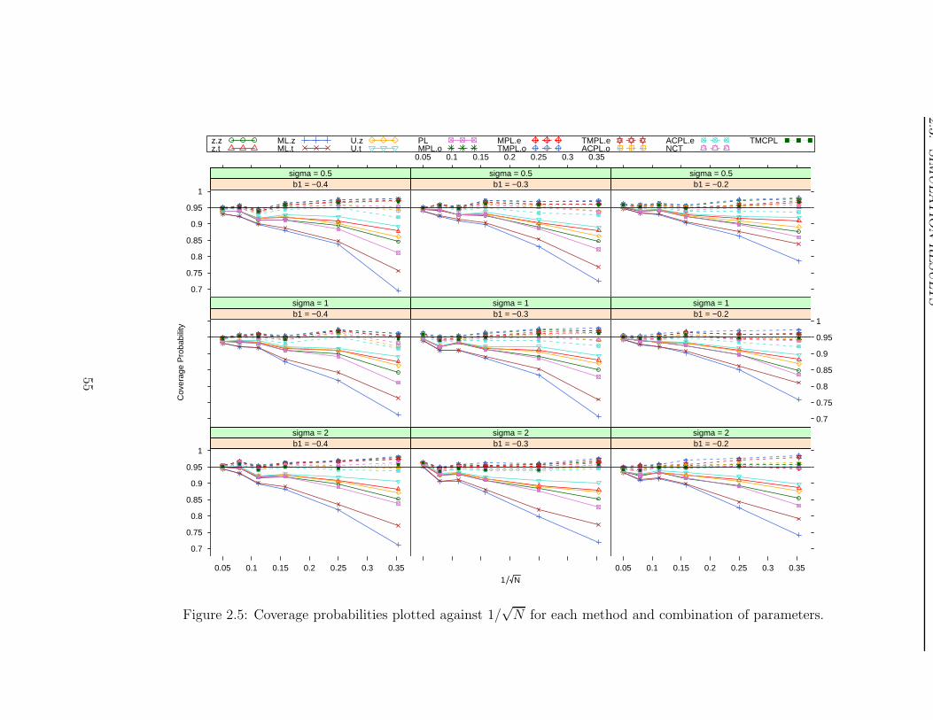
2.3
.SIM
ULA
TIO
NR
ESU
LT
S
1 N
Cov
erag
e P
roba
bilit
y
0.7
0.75
0.8
0.85
0.9
0.95
1b1 = −0.4
sigma = 0.5b1 = −0.3
sigma = 0.5
0.05 0.1 0.15 0.2 0.25 0.3 0.35
b1 = −0.2sigma = 0.5
b1 = −0.4sigma = 1
b1 = −0.3sigma = 1
0.7
0.75
0.8
0.85
0.9
0.95
1b1 = −0.2sigma = 1
0.7
0.75
0.8
0.85
0.9
0.95
1
0.05 0.1 0.15 0.2 0.25 0.3 0.35
b1 = −0.4sigma = 2
b1 = −0.3sigma = 2
0.05 0.1 0.15 0.2 0.25 0.3 0.35
b1 = −0.2sigma = 2
z.zz.t
ML.zML.t
U.zU.t
PLMPL.o
MPL.eTMPL.o
TMPL.eACPL.o
ACPL.eNCT
TMCPL
Figure 2.5: Coverage probabilities plotted against 1/√N for each method and combination of parameters.
55
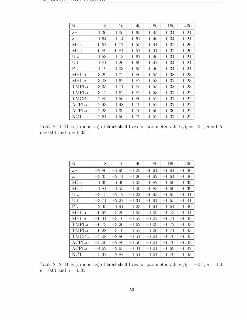
2.3. SIMULATION RESULTS
N 8 16 40 80 160 400
z.z −1.36 −1.06 −0.65 −0.45 −0.34 −0.21z.t −1.64 −1.14 −0.67 −0.46 −0.34 −0.21ML.z −0.67 −0.77 −0.55 −0.41 −0.32 −0.20ML.t −0.89 −0.84 −0.57 −0.41 −0.32 −0.20U.z −1.53 −1.13 −0.67 −0.46 −0.34 −0.21U.t −1.81 −1.20 −0.69 −0.47 −0.34 −0.21PL −1.19 −1.03 −0.65 −0.46 −0.34 −0.21MPL.o −3.29 −1.72 −0.86 −0.55 −0.38 −0.23MPL.e −3.08 −1.62 −0.82 −0.53 −0.37 −0.23TMPL.o −3.35 −1.71 −0.85 −0.55 −0.38 −0.23TMPL.e −3.12 −1.62 −0.82 −0.53 −0.37 −0.22TMCPL −2.85 −1.56 −0.80 −0.52 −0.37 −0.22ACPL.o −2.43 −1.48 −0.79 −0.52 −0.37 −0.22ACPL.e −2.23 −1.39 −0.76 −0.50 −0.36 −0.22NCT −2.61 −1.50 −0.79 −0.52 −0.37 −0.22
Table 2.11: Bias (in months) of label shelf-lives for parameter values β1 = −0.4, σ = 0.5,ε = 0.01 and α = 0.05.
N 8 16 40 80 160 400
z.z −2.80 −1.99 −1.23 −0.91 −0.64 −0.40z.t −3.35 −2.14 −1.26 −0.92 −0.64 −0.40ML.z −1.39 −1.40 −1.03 −0.82 −0.60 −0.39ML.t −1.81 −1.53 −1.06 −0.83 −0.60 −0.39U.z −3.15 −2.12 −1.28 −0.93 −0.65 −0.41U.t −3.71 −2.27 −1.31 −0.94 −0.65 −0.41PL −2.43 −1.91 −1.23 −0.91 −0.64 −0.40MPL.o −6.92 −3.26 −1.63 −1.09 −0.73 −0.44MPL.e −6.41 −3.10 −1.57 −1.07 −0.71 −0.43TMPL.o −6.73 −3.26 −1.62 −1.09 −0.72 −0.43TMPL.e −6.28 −3.10 −1.57 −1.06 −0.71 −0.43TMCPL −5.08 −2.86 −1.51 −1.04 −0.70 −0.43ACPL.o −5.00 −2.80 −1.50 −1.04 −0.70 −0.43ACPL.e −4.62 −2.65 −1.44 −1.01 −0.69 −0.42NCT −5.37 −2.87 −1.51 −1.04 −0.70 −0.43
Table 2.12: Bias (in months) of label shelf-lives for parameter values β1 = −0.4, σ = 1.0,ε = 0.01 and α = 0.05.
56

2.3. SIMULATION RESULTS
N 8 16 40 80 160 400
z.z −5.83 −4.06 −2.49 −1.73 −1.29 −0.83z.t −6.78 −4.37 −2.56 −1.75 −1.30 −0.83ML.z −3.13 −2.82 −2.08 −1.54 −1.20 −0.79ML.t −4.01 −3.10 −2.14 −1.56 −1.21 −0.79U.z −6.41 −4.33 −2.58 −1.77 −1.31 −0.83U.t −7.34 −4.64 −2.65 −1.79 −1.32 −0.84PL −5.19 −3.90 −2.48 −1.73 −1.29 −0.83MPL.o −11.00 −6.99 −3.36 −2.11 −1.46 −0.89MPL.e −10.51 −6.54 −3.24 −2.06 −1.44 −0.88TMPL.o −10.45 −6.49 −3.26 −2.07 −1.45 −0.89TMPL.e −9.90 −6.08 −3.14 −2.02 −1.43 −0.88TMCPL −6.45 −4.59 −2.79 −1.89 −1.37 −0.86ACPL.o −9.26 −5.83 −3.05 −1.98 −1.41 −0.87ACPL.e −8.65 −5.44 −2.94 −1.93 −1.38 −0.86NCT −9.40 −5.86 −3.07 −1.99 −1.41 −0.87
Table 2.13: Bias (in months) of label shelf-lives for parameter values β1 = −0.4, σ = 2.0,ε = 0.01 and α = 0.05.
N 8 16 40 80 160 400
z.z −2.00 −1.48 −0.99 −0.69 −0.50 −0.33z.t −2.39 −1.59 −1.02 −0.70 −0.50 −0.33ML.z −1.08 −1.09 −0.86 −0.63 −0.47 −0.32ML.t −1.40 −1.19 −0.88 −0.64 −0.47 −0.32U.z −2.21 −1.56 −1.02 −0.71 −0.51 −0.33U.t −2.61 −1.67 −1.05 −0.72 −0.51 −0.33PL −1.78 −1.44 −0.99 −0.70 −0.50 −0.33MPL.o −4.63 −2.41 −1.29 −0.83 −0.56 −0.35MPL.e −4.23 −2.23 −1.23 −0.80 −0.55 −0.35TMPL.o −4.93 −2.44 −1.29 −0.83 −0.56 −0.35TMPL.e −4.49 −2.25 −1.23 −0.80 −0.55 −0.35TMCPL −4.09 −2.17 −1.21 −0.79 −0.55 −0.34ACPL.o −3.57 −2.10 −1.20 −0.79 −0.55 −0.34ACPL.e −3.19 −1.92 −1.14 −0.76 −0.53 −0.34NCT −3.64 −2.06 −1.18 −0.78 −0.54 −0.34
Table 2.14: Bias (in months) of label shelf-lives for parameter values β1 = −0.3, σ = 0.5,ε = 0.01 and α = 0.05.
57
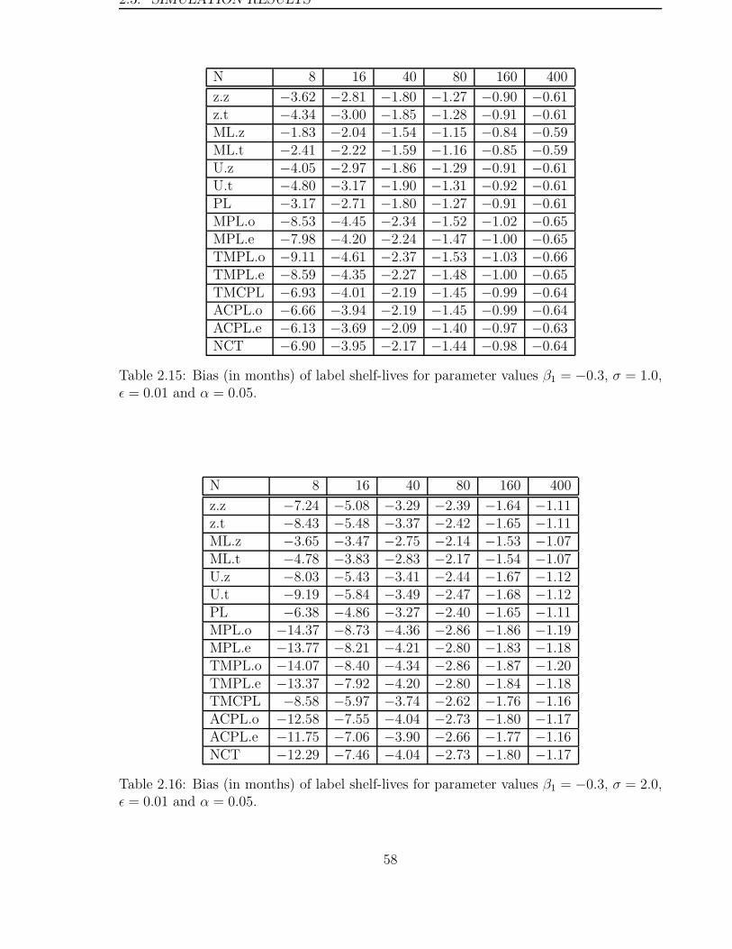
2.3. SIMULATION RESULTS
N 8 16 40 80 160 400
z.z −3.62 −2.81 −1.80 −1.27 −0.90 −0.61z.t −4.34 −3.00 −1.85 −1.28 −0.91 −0.61ML.z −1.83 −2.04 −1.54 −1.15 −0.84 −0.59ML.t −2.41 −2.22 −1.59 −1.16 −0.85 −0.59U.z −4.05 −2.97 −1.86 −1.29 −0.91 −0.61U.t −4.80 −3.17 −1.90 −1.31 −0.92 −0.61PL −3.17 −2.71 −1.80 −1.27 −0.91 −0.61MPL.o −8.53 −4.45 −2.34 −1.52 −1.02 −0.65MPL.e −7.98 −4.20 −2.24 −1.47 −1.00 −0.65TMPL.o −9.11 −4.61 −2.37 −1.53 −1.03 −0.66TMPL.e −8.59 −4.35 −2.27 −1.48 −1.00 −0.65TMCPL −6.93 −4.01 −2.19 −1.45 −0.99 −0.64ACPL.o −6.66 −3.94 −2.19 −1.45 −0.99 −0.64ACPL.e −6.13 −3.69 −2.09 −1.40 −0.97 −0.63NCT −6.90 −3.95 −2.17 −1.44 −0.98 −0.64
Table 2.15: Bias (in months) of label shelf-lives for parameter values β1 = −0.3, σ = 1.0,ε = 0.01 and α = 0.05.
N 8 16 40 80 160 400
z.z −7.24 −5.08 −3.29 −2.39 −1.64 −1.11z.t −8.43 −5.48 −3.37 −2.42 −1.65 −1.11ML.z −3.65 −3.47 −2.75 −2.14 −1.53 −1.07ML.t −4.78 −3.83 −2.83 −2.17 −1.54 −1.07U.z −8.03 −5.43 −3.41 −2.44 −1.67 −1.12U.t −9.19 −5.84 −3.49 −2.47 −1.68 −1.12PL −6.38 −4.86 −3.27 −2.40 −1.65 −1.11MPL.o −14.37 −8.73 −4.36 −2.86 −1.86 −1.19MPL.e −13.77 −8.21 −4.21 −2.80 −1.83 −1.18TMPL.o −14.07 −8.40 −4.34 −2.86 −1.87 −1.20TMPL.e −13.37 −7.92 −4.20 −2.80 −1.84 −1.18TMCPL −8.58 −5.97 −3.74 −2.62 −1.76 −1.16ACPL.o −12.58 −7.55 −4.04 −2.73 −1.80 −1.17ACPL.e −11.75 −7.06 −3.90 −2.66 −1.77 −1.16NCT −12.29 −7.46 −4.04 −2.73 −1.80 −1.17
Table 2.16: Bias (in months) of label shelf-lives for parameter values β1 = −0.3, σ = 2.0,ε = 0.01 and α = 0.05.
58
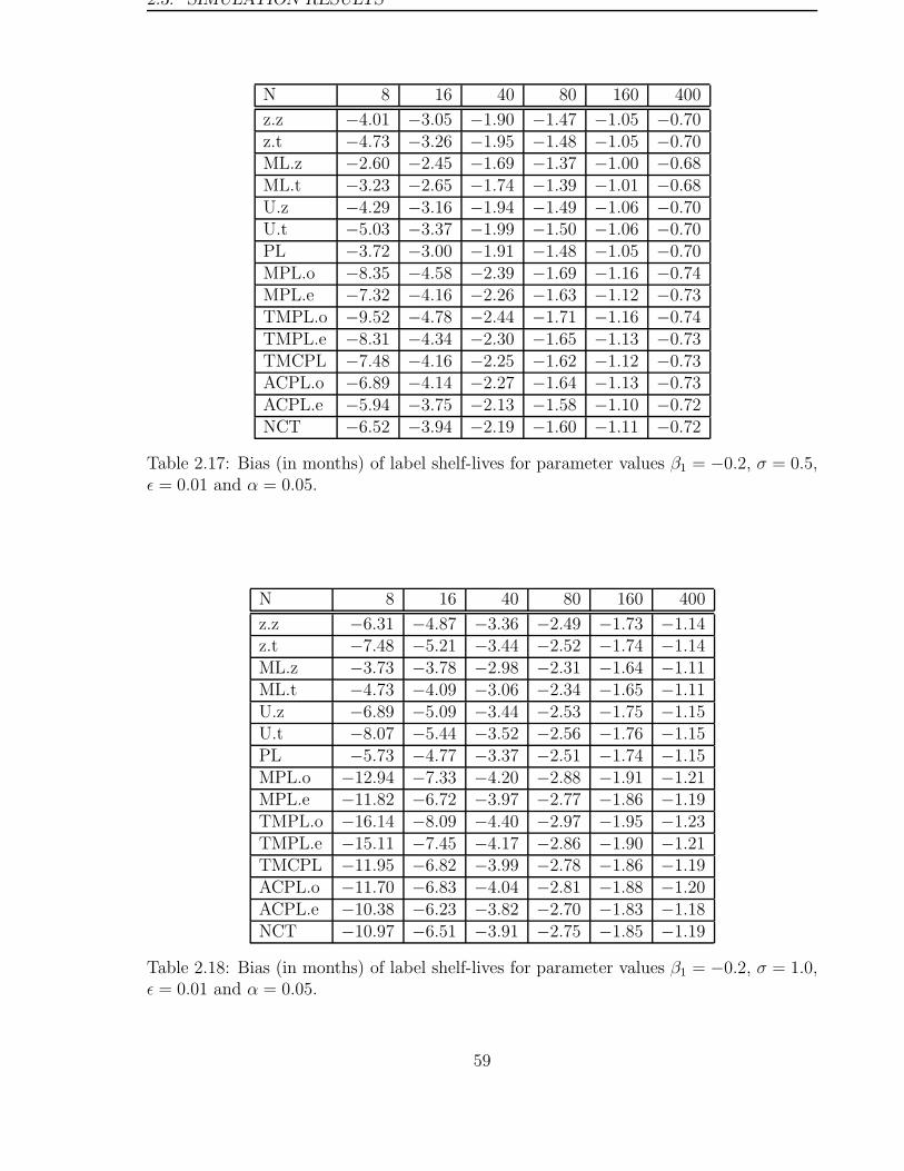
2.3. SIMULATION RESULTS
N 8 16 40 80 160 400
z.z −4.01 −3.05 −1.90 −1.47 −1.05 −0.70z.t −4.73 −3.26 −1.95 −1.48 −1.05 −0.70ML.z −2.60 −2.45 −1.69 −1.37 −1.00 −0.68ML.t −3.23 −2.65 −1.74 −1.39 −1.01 −0.68U.z −4.29 −3.16 −1.94 −1.49 −1.06 −0.70U.t −5.03 −3.37 −1.99 −1.50 −1.06 −0.70PL −3.72 −3.00 −1.91 −1.48 −1.05 −0.70MPL.o −8.35 −4.58 −2.39 −1.69 −1.16 −0.74MPL.e −7.32 −4.16 −2.26 −1.63 −1.12 −0.73TMPL.o −9.52 −4.78 −2.44 −1.71 −1.16 −0.74TMPL.e −8.31 −4.34 −2.30 −1.65 −1.13 −0.73TMCPL −7.48 −4.16 −2.25 −1.62 −1.12 −0.73ACPL.o −6.89 −4.14 −2.27 −1.64 −1.13 −0.73ACPL.e −5.94 −3.75 −2.13 −1.58 −1.10 −0.72NCT −6.52 −3.94 −2.19 −1.60 −1.11 −0.72
Table 2.17: Bias (in months) of label shelf-lives for parameter values β1 = −0.2, σ = 0.5,ε = 0.01 and α = 0.05.
N 8 16 40 80 160 400
z.z −6.31 −4.87 −3.36 −2.49 −1.73 −1.14z.t −7.48 −5.21 −3.44 −2.52 −1.74 −1.14ML.z −3.73 −3.78 −2.98 −2.31 −1.64 −1.11ML.t −4.73 −4.09 −3.06 −2.34 −1.65 −1.11U.z −6.89 −5.09 −3.44 −2.53 −1.75 −1.15U.t −8.07 −5.44 −3.52 −2.56 −1.76 −1.15PL −5.73 −4.77 −3.37 −2.51 −1.74 −1.15MPL.o −12.94 −7.33 −4.20 −2.88 −1.91 −1.21MPL.e −11.82 −6.72 −3.97 −2.77 −1.86 −1.19TMPL.o −16.14 −8.09 −4.40 −2.97 −1.95 −1.23TMPL.e −15.11 −7.45 −4.17 −2.86 −1.90 −1.21TMCPL −11.95 −6.82 −3.99 −2.78 −1.86 −1.19ACPL.o −11.70 −6.83 −4.04 −2.81 −1.88 −1.20ACPL.e −10.38 −6.23 −3.82 −2.70 −1.83 −1.18NCT −10.97 −6.51 −3.91 −2.75 −1.85 −1.19
Table 2.18: Bias (in months) of label shelf-lives for parameter values β1 = −0.2, σ = 1.0,ε = 0.01 and α = 0.05.
59
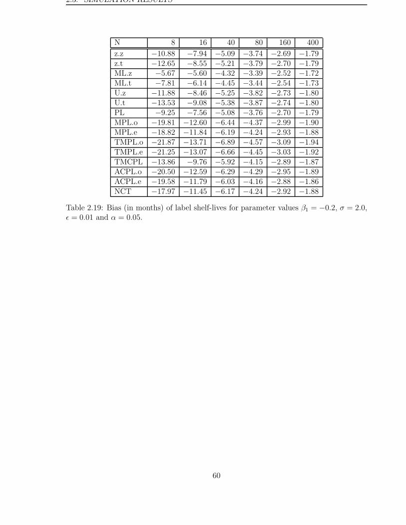
2.3. SIMULATION RESULTS
N 8 16 40 80 160 400
z.z −10.88 −7.94 −5.09 −3.74 −2.69 −1.79z.t −12.65 −8.55 −5.21 −3.79 −2.70 −1.79ML.z −5.67 −5.60 −4.32 −3.39 −2.52 −1.72ML.t −7.81 −6.14 −4.45 −3.44 −2.54 −1.73U.z −11.88 −8.46 −5.25 −3.82 −2.73 −1.80U.t −13.53 −9.08 −5.38 −3.87 −2.74 −1.80PL −9.25 −7.56 −5.08 −3.76 −2.70 −1.79MPL.o −19.81 −12.60 −6.44 −4.37 −2.99 −1.90MPL.e −18.82 −11.84 −6.19 −4.24 −2.93 −1.88TMPL.o −21.87 −13.71 −6.89 −4.57 −3.09 −1.94TMPL.e −21.25 −13.07 −6.66 −4.45 −3.03 −1.92TMCPL −13.86 −9.76 −5.92 −4.15 −2.89 −1.87ACPL.o −20.50 −12.59 −6.29 −4.29 −2.95 −1.89ACPL.e −19.58 −11.79 −6.03 −4.16 −2.88 −1.86NCT −17.97 −11.45 −6.17 −4.24 −2.92 −1.88
Table 2.19: Bias (in months) of label shelf-lives for parameter values β1 = −0.2, σ = 2.0,ε = 0.01 and α = 0.05.
60
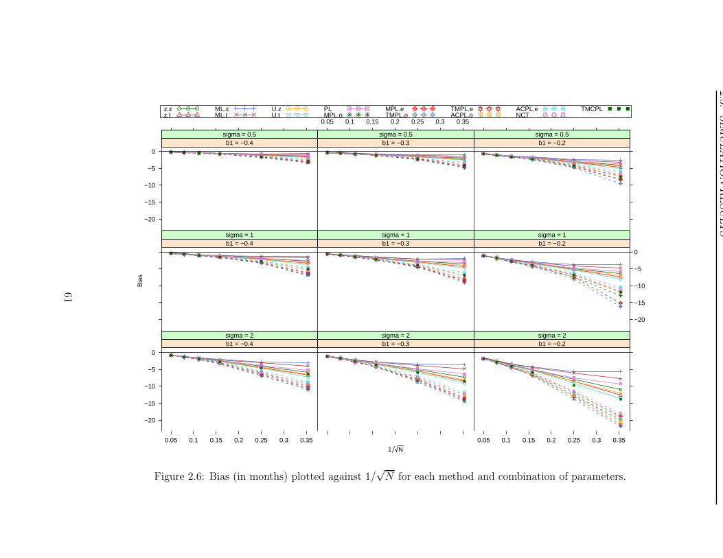
2.3
.SIM
ULA
TIO
NR
ESU
LT
S
1 N
Bia
s
−20
−15
−10
−5
0b1 = −0.4
sigma = 0.5b1 = −0.3
sigma = 0.5
0.05 0.1 0.15 0.2 0.25 0.3 0.35
b1 = −0.2sigma = 0.5
b1 = −0.4sigma = 1
b1 = −0.3sigma = 1
−20
−15
−10
−5
0b1 = −0.2sigma = 1
−20
−15
−10
−5
0
0.05 0.1 0.15 0.2 0.25 0.3 0.35
b1 = −0.4sigma = 2
b1 = −0.3sigma = 2
0.05 0.1 0.15 0.2 0.25 0.3 0.35
b1 = −0.2sigma = 2
z.zz.t
ML.zML.t
U.zU.t
PLMPL.o
MPL.eTMPL.o
TMPL.eACPL.o
ACPL.eNCT
TMCPL
Figure 2.6: Bias (in months) plotted against 1/√N for each method and combination of parameters.
61
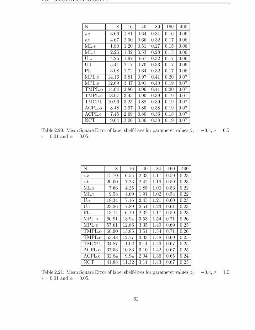
2.3. SIMULATION RESULTS
N 8 16 40 80 160 400
z.z 3.66 1.81 0.64 0.31 0.16 0.06z.t 4.67 2.00 0.66 0.32 0.17 0.06ML.z 1.80 1.20 0.51 0.27 0.15 0.06ML.t 2.26 1.32 0.53 0.28 0.15 0.06U.z 4.26 1.97 0.67 0.32 0.17 0.06U.t 5.41 2.17 0.70 0.33 0.17 0.06PL 3.08 1.72 0.64 0.32 0.17 0.06MPL.o 14.16 3.81 0.97 0.41 0.20 0.07MPL.e 12.69 3.47 0.91 0.40 0.19 0.07TMPL.o 14.64 3.80 0.96 0.41 0.20 0.07TMPL.e 13.07 3.45 0.90 0.39 0.19 0.07TMCPL 10.96 3.25 0.88 0.39 0.19 0.07ACPL.o 8.48 2.97 0.85 0.38 0.19 0.07ACPL.e 7.45 2.69 0.80 0.36 0.18 0.07NCT 9.64 3.06 0.86 0.38 0.19 0.07
Table 2.20: Mean Square Error of label shelf-lives for parameter values β1 = −0.4, σ = 0.5,ε = 0.01 and α = 0.05.
N 8 16 40 80 160 400
z.z 15.70 6.55 2.33 1.17 0.59 0.23z.t 20.00 7.23 2.42 1.19 0.59 0.23ML.z 7.66 4.25 1.85 1.00 0.53 0.22ML.t 9.58 4.69 1.91 1.02 0.54 0.22U.z 18.34 7.16 2.45 1.21 0.60 0.23U.t 23.26 7.89 2.54 1.23 0.61 0.23PL 13.14 6.19 2.32 1.17 0.59 0.23MPL.o 66.91 13.94 3.53 1.54 0.71 0.26MPL.e 57.61 12.86 3.35 1.49 0.69 0.25TMPL.o 60.90 13.85 3.51 1.54 0.71 0.26TMPL.e 53.48 12.77 3.33 1.48 0.69 0.25TMCPL 34.87 11.02 3.14 1.43 0.67 0.25ACPL.o 37.53 10.83 3.10 1.42 0.67 0.25ACPL.e 32.84 9.94 2.94 1.36 0.65 0.24NCT 41.88 11.32 3.14 1.43 0.67 0.25
Table 2.21: Mean Square Error of label shelf-lives for parameter values β1 = −0.4, σ = 1.0,ε = 0.01 and α = 0.05.
62
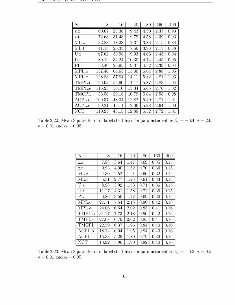
2.3. SIMULATION RESULTS
N 8 16 40 80 160 400
z.z 60.67 28.38 9.43 4.50 2.37 0.93z.t 72.68 31.43 9.79 4.58 2.39 0.93ML.z 32.83 18.28 7.37 3.86 2.15 0.88ML.t 41.13 20.33 7.66 3.93 2.17 0.88U.z 67.62 30.98 9.93 4.66 2.43 0.94U.t 80.19 34.24 10.30 4.74 2.45 0.95PL 53.40 26.95 9.37 4.52 2.39 0.94MPL.o 137.46 64.65 15.00 6.04 2.88 1.05MPL.e 128.83 57.84 14.11 5.82 2.81 1.03TMPL.o 126.03 55.90 14.17 5.87 2.83 1.04TMPL.e 116.23 50.10 13.34 5.65 2.76 1.02TMCPL 53.56 29.18 10.79 5.04 2.58 0.98ACPL.o 109.37 48.34 12.82 5.49 2.71 1.01ACPL.e 99.21 43.11 12.06 5.28 2.64 1.00NCT 110.23 48.15 12.89 5.52 2.72 1.01
Table 2.22: Mean Square Error of label shelf-lives for parameter values β1 = −0.4, σ = 2.0,ε = 0.01 and α = 0.05.
N 8 16 40 80 160 400
z.z 7.88 3.64 1.47 0.69 0.35 0.15z.t 9.93 4.00 1.52 0.70 0.36 0.15ML.z 4.30 2.52 1.21 0.60 0.32 0.14ML.t 5.31 2.77 1.25 0.61 0.33 0.14U.z 8.98 3.92 1.53 0.71 0.36 0.15U.t 11.27 4.31 1.58 0.72 0.36 0.15PL 6.86 3.50 1.47 0.69 0.36 0.15MPL.o 27.71 7.54 2.18 0.90 0.42 0.16MPL.e 24.06 6.64 2.02 0.85 0.41 0.16TMPL.o 31.27 7.73 2.18 0.90 0.42 0.16TMPL.e 27.08 6.79 2.02 0.85 0.41 0.16TMCPL 22.59 6.37 1.96 0.84 0.40 0.16ACPL.o 18.12 6.04 1.95 0.84 0.40 0.16ACPL.e 15.33 5.29 1.80 0.79 0.39 0.16NCT 18.92 5.90 1.90 0.82 0.40 0.16
Table 2.23: Mean Square Error of label shelf-lives for parameter values β1 = −0.3, σ = 0.5,ε = 0.01 and α = 0.05.
63
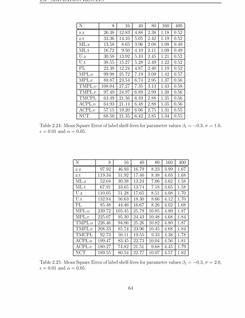
2.3. SIMULATION RESULTS
N 8 16 40 80 160 400
z.z 26.38 12.83 4.88 2.38 1.18 0.52z.t 33.36 14.10 5.05 2.42 1.19 0.52ML.z 13.58 8.65 3.96 2.08 1.08 0.49ML.t 16.72 9.50 4.10 2.11 1.09 0.49U.z 30.58 13.92 5.10 2.45 1.21 0.52U.t 38.55 15.27 5.28 2.49 1.22 0.52PL 22.38 12.24 4.87 2.40 1.19 0.52MPL.o 99.98 25.72 7.19 3.09 1.42 0.57MPL.e 88.87 23.54 6.74 2.95 1.37 0.56TMPL.o 108.04 27.27 7.35 3.13 1.43 0.58TMPL.e 97.49 24.97 6.89 2.99 1.38 0.56TMCPL 63.49 21.56 6.49 2.88 1.35 0.56ACPL.o 64.93 21.14 6.48 2.88 1.35 0.56ACPL.e 57.15 19.20 6.06 2.75 1.31 0.55NCT 68.50 21.35 6.42 2.85 1.34 0.55
Table 2.24: Mean Square Error of label shelf-lives for parameter values β1 = −0.3, σ = 1.0,ε = 0.01 and α = 0.05.
N 8 16 40 80 160 400
z.z 97.92 46.93 16.79 8.23 3.99 1.67z.t 119.34 51.92 17.40 8.38 4.03 1.68ML.z 52.04 30.38 13.24 7.06 3.62 1.58ML.t 67.91 33.65 13.74 7.18 3.65 1.58U.z 110.05 51.28 17.65 8.51 4.08 1.70U.t 132.84 56.63 18.30 8.66 4.12 1.70PL 85.48 44.46 16.67 8.26 4.02 1.68MPL.o 239.72 105.45 25.79 10.85 4.80 1.87MPL.e 225.07 95.30 24.43 10.48 4.68 1.84TMPL.o 226.46 94.86 25.26 10.82 4.80 1.87TMPL.e 208.33 85.74 23.96 10.45 4.68 1.84TMCPL 92.73 50.11 19.55 9.33 4.38 1.78ACPL.o 199.47 83.45 22.73 10.04 4.56 1.81ACPL.e 180.27 74.82 21.51 9.68 4.45 1.79NCT 189.55 80.54 22.77 10.07 4.57 1.82
Table 2.25: Mean Square Error of label shelf-lives for parameter values β1 = −0.3, σ = 2.0,ε = 0.01 and α = 0.05.
64
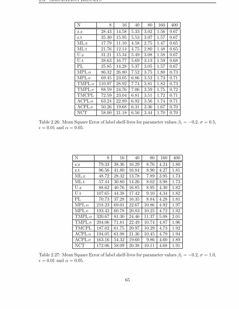
2.3. SIMULATION RESULTS
N 8 16 40 80 160 400
z.z 28.43 14.58 5.33 3.02 1.56 0.67z.t 35.30 15.95 5.53 3.07 1.57 0.67ML.z 17.79 11.10 4.58 2.75 1.47 0.65ML.t 21.76 12.14 4.75 2.80 1.48 0.65U.z 31.21 15.34 5.49 3.08 1.58 0.67U.t 38.63 16.77 5.69 3.13 1.59 0.68PL 25.85 14.28 5.37 3.05 1.57 0.67MPL.o 86.32 26.80 7.52 3.75 1.80 0.73MPL.e 69.45 23.05 6.86 3.53 1.73 0.71TMPL.o 110.97 28.92 7.74 3.81 1.82 0.73TMPL.e 88.59 24.76 7.06 3.59 1.75 0.72TMCPL 72.59 23.04 6.81 3.51 1.72 0.71ACPL.o 63.24 22.89 6.92 3.56 1.74 0.71ACPL.e 50.26 19.68 6.31 3.36 1.67 0.70NCT 58.00 21.18 6.56 3.44 1.70 0.70
Table 2.26: Mean Square Error of label shelf-lives for parameter values β1 = −0.2, σ = 0.5,ε = 0.01 and α = 0.05.
N 8 16 40 80 160 400
z.z 79.33 38.36 16.29 8.76 4.24 1.80z.t 96.56 41.80 16.84 8.90 4.27 1.81ML.z 48.72 28.32 13.78 7.89 3.95 1.73ML.t 57.44 30.80 14.26 8.02 3.98 1.73U.z 88.62 40.76 16.85 8.95 4.30 1.82U.t 107.65 44.38 17.42 9.10 4.34 1.82PL 70.73 37.28 16.35 8.84 4.28 1.81MPL.o 218.23 69.01 22.67 10.86 4.92 1.97MPL.e 193.42 60.78 20.83 10.25 4.72 1.92TMPL.o 320.67 81.30 24.46 11.37 5.08 2.01TMPL.e 294.06 71.81 22.49 10.74 4.87 1.96TMCPL 187.02 61.75 20.97 10.29 4.73 1.92ACPL.o 194.05 61.98 21.36 10.45 4.79 1.94ACPL.e 163.16 54.32 19.60 9.86 4.60 1.89NCT 172.06 58.09 20.38 10.11 4.68 1.91
Table 2.27: Mean Square Error of label shelf-lives for parameter values β1 = −0.2, σ = 1.0,ε = 0.01 and α = 0.05.
65
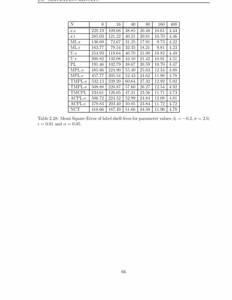
2.3. SIMULATION RESULTS
N 8 16 40 80 160 400
z.z 229.19 109.68 38.85 20.48 10.61 4.44z.t 285.03 121.22 40.21 20.81 10.70 4.46ML.z 136.69 72.67 31.25 17.91 9.73 4.22ML.t 163.77 79.54 32.35 18.21 9.81 4.23U.z 254.93 119.64 40.70 21.08 10.82 4.49U.t 300.82 132.08 42.10 21.42 10.91 4.51PL 191.46 102.79 38.67 20.59 10.70 4.47MPL.o 485.86 224.90 55.40 25.63 12.34 4.88MPL.e 457.77 205.54 52.43 24.62 11.98 4.78TMPL.o 532.13 239.20 60.64 27.32 12.92 5.02TMPL.e 508.88 220.87 57.60 26.27 12.54 4.92TMCPL 234.61 126.65 47.21 23.56 11.71 4.73ACPL.o 506.72 224.52 52.99 24.84 12.08 4.81ACPL.e 479.83 203.40 50.05 23.84 11.72 4.72NCT 418.66 187.49 51.66 24.50 11.96 4.78
Table 2.28: Mean Square Error of label shelf-lives for parameter values β1 = −0.2, σ = 2.0,ε = 0.01 and α = 0.05.
66
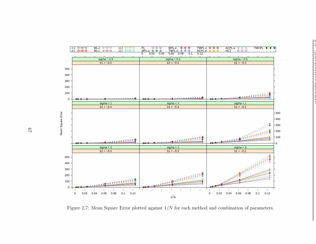
2.3
.SIM
ULA
TIO
NR
ESU
LT
S
1 N
Mea
n S
quar
e E
rror
0
100
200
300
400
500
b1 = −0.4sigma = 0.5
b1 = −0.3sigma = 0.5
0 0.02 0.04 0.06 0.08 0.1 0.12
b1 = −0.2sigma = 0.5
b1 = −0.4sigma = 1
b1 = −0.3sigma = 1
0
100
200
300
400
500
b1 = −0.2sigma = 1
0
100
200
300
400
500
0 0.02 0.04 0.06 0.08 0.1 0.12
b1 = −0.4sigma = 2
b1 = −0.3sigma = 2
0 0.02 0.04 0.06 0.08 0.1 0.12
b1 = −0.2sigma = 2
z.zz.t
ML.zML.t
U.zU.t
PLMPL.o
MPL.eTMPL.o
TMPL.eACPL.o
ACPL.eNCT
TMCPL
Figure 2.7: Mean Square Error plotted against 1/N for each method and combination of parameters.
67
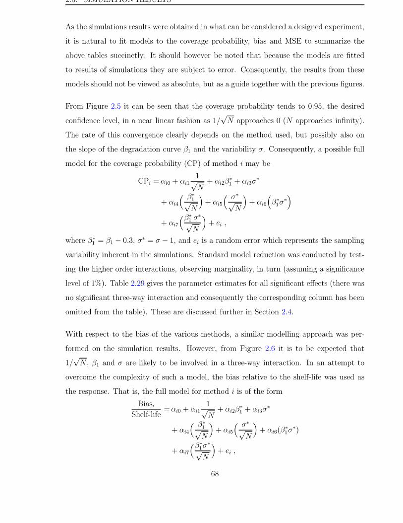
2.3. SIMULATION RESULTS
As the simulations results were obtained in what can be considered a designed experiment,
it is natural to fit models to the coverage probability, bias and MSE to summarize the
above tables succinctly. It should however be noted that because the models are fitted
to results of simulations they are subject to error. Consequently, the results from these
models should not be viewed as absolute, but as a guide together with the previous figures.
From Figure 2.5 it can be seen that the coverage probability tends to 0.95, the desired
confidence level, in a near linear fashion as 1/√N approaches 0 (N approaches infinity).
The rate of this convergence clearly depends on the method used, but possibly also on
the slope of the degradation curve β1 and the variability σ. Consequently, a possible full
model for the coverage probability (CP) of method i may be
CPi =αi0 + αi11√N
+ αi2β∗1 + αi3σ
∗
+ αi4
( β∗1√N
)
+ αi5
( σ∗
√N
)
+ αi6
(
β∗1σ
∗)
+ αi7
(β∗1 σ
∗
√N
)
+ ei ,
where β∗1 = β1 − 0.3, σ∗ = σ − 1, and ei is a random error which represents the sampling
variability inherent in the simulations. Standard model reduction was conducted by test-
ing the higher order interactions, observing marginality, in turn (assuming a significance
level of 1%). Table 2.29 gives the parameter estimates for all significant effects (there was
no significant three-way interaction and consequently the corresponding column has been
omitted from the table). These are discussed further in Section 2.4.
With respect to the bias of the various methods, a similar modelling approach was per-
formed on the simulation results. However, from Figure 2.6 it is to be expected that
1/√N , β1 and σ are likely to be involved in a three-way interaction. In an attempt to
overcome the complexity of such a model, the bias relative to the shelf-life was used as
the response. That is, the full model for method i is of the form
Biasi
Shelf-life=αi0 + αi1
1√N
+ αi2β∗1 + αi3σ
∗
+ αi4
( β∗1√N
)
+ αi5
( σ∗
√N
)
+ αi6(β∗1σ
∗)
+ αi7
(β∗1σ
∗
√N
)
+ ei ,
68
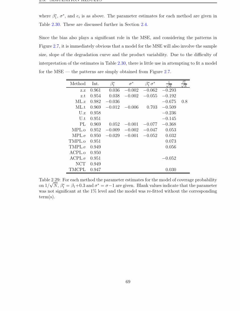
2.3. SIMULATION RESULTS
where β∗1 , σ
∗, and ei is as above. The parameter estimates for each method are given in
Table 2.30. These are discussed further in Section 2.4.
Since the bias also plays a significant role in the MSE, and considering the patterns in
Figure 2.7, it is immediately obvious that a model for the MSE will also involve the sample
size, slope of the degradation curve and the product variability. Due to the difficulty of
interpretation of the estimates in Table 2.30, there is little use in attempting to fit a model
for the MSE — the patterns are simply obtained from Figure 2.7.
Method Int. β∗1 σ∗ β∗
1 σ∗ 1√
N
β∗
1√N
z.z 0.961 0.036 −0.002 −0.062 −0.293z.t 0.954 0.038 −0.002 −0.055 −0.192
ML.z 0.982 −0.036 −0.675 0.8ML.t 0.969 −0.012 −0.006 0.703 −0.509
U.z 0.958 −0.236U.t 0.951 −0.145PL 0.969 0.052 −0.001 −0.077 −0.368
MPL.o 0.952 −0.009 −0.002 −0.047 0.053MPL.e 0.950 −0.029 −0.001 −0.052 0.032
TMPL.o 0.951 0.073TMPL.e 0.949 0.056ACPL.o 0.950ACPL.e 0.951 −0.052
NCT 0.949TMCPL 0.947 0.030
Table 2.29: For each method the parameter estimates for the model of coverage probabilityon 1/
√N , β∗
1 = β1+0.3 and σ∗ = σ−1 are given. Blank values indicate that the parameterwas not significant at the 1% level and the model was re-fitted without the correspondingterm(s).
69
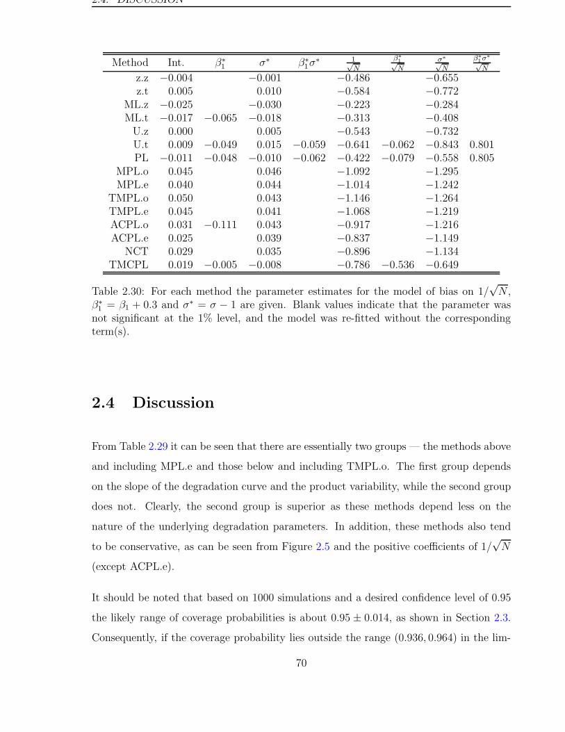
2.4. DISCUSSION
Method Int. β∗1 σ∗ β∗
1σ∗ 1√
N
β∗
1√N
σ∗
√N
β∗
1σ∗
√N
z.z −0.004 −0.001 −0.486 −0.655z.t 0.005 0.010 −0.584 −0.772
ML.z −0.025 −0.030 −0.223 −0.284ML.t −0.017 −0.065 −0.018 −0.313 −0.408
U.z 0.000 0.005 −0.543 −0.732U.t 0.009 −0.049 0.015 −0.059 −0.641 −0.062 −0.843 0.801PL −0.011 −0.048 −0.010 −0.062 −0.422 −0.079 −0.558 0.805
MPL.o 0.045 0.046 −1.092 −1.295MPL.e 0.040 0.044 −1.014 −1.242
TMPL.o 0.050 0.043 −1.146 −1.264TMPL.e 0.045 0.041 −1.068 −1.219ACPL.o 0.031 −0.111 0.043 −0.917 −1.216ACPL.e 0.025 0.039 −0.837 −1.149
NCT 0.029 0.035 −0.896 −1.134TMCPL 0.019 −0.005 −0.008 −0.786 −0.536 −0.649
Table 2.30: For each method the parameter estimates for the model of bias on 1/√N ,
β∗1 = β1 + 0.3 and σ∗ = σ − 1 are given. Blank values indicate that the parameter was
not significant at the 1% level, and the model was re-fitted without the correspondingterm(s).
2.4 Discussion
From Table 2.29 it can be seen that there are essentially two groups — the methods above
and including MPL.e and those below and including TMPL.o. The first group depends
on the slope of the degradation curve and the product variability, while the second group
does not. Clearly, the second group is superior as these methods depend less on the
nature of the underlying degradation parameters. In addition, these methods also tend
to be conservative, as can be seen from Figure 2.5 and the positive coefficients of 1/√N
(except ACPL.e).
It should be noted that based on 1000 simulations and a desired confidence level of 0.95
the likely range of coverage probabilities is about 0.95 ± 0.014, as shown in Section 2.3.
Consequently, if the coverage probability lies outside the range (0.936, 0.964) in the lim-
70

2.4. DISCUSSION
iting case as N → ∞, then the true limiting coverage probability is likely to differ from
0.95. However, for some methods the intercept may lie outside these limit because higher
order terms, such as 1/N3/2, were omitted from the already complex models. Including
such a term may reduce the intercept to a level that it is not significantly different from
0.95.
From the tables and graphs in Section 2.3 the following general statements can be made.
• The coverage probability tends toward 0.95 as N → ∞ for all methods. Some
methods appear to depend on the degradation parameters more than others;
• The bias and MSE tend toward zero as N → ∞. The rate at which different
methods reduce in bias depends on the sample size, the slope of the degradation
curve and the product variability, as can be seen from Figure 2.6 and Table 2.30;
• Smaller coefficients of 1/√N indicate that the corresponding method works better
for small sample sizes;
• Larger variability, as indicated by larger values of σ, tends to result in larger bias
and MSE;
• Slower degradation, as indicated by smaller (absolute) values of β1, also tends to
result in larger bias and MSE.
• Methods with lower coverage probabilities tend to also exhibit smaller bias and
MSE. This is not surprising as all three measures suggest that the label shelf-life is
too large. However, coverage probability is the most important of these three perfor-
mance criteria. Methods with roughly equal coverage can then be further compared
by their bias and MSE. Consequently, unless mentioned otherwise, performance will
hereafter refer to coverage probability.
The approaches based on the normal approximation under-performed with respect to
coverage probability for all values of β1 and σ that were chosen for the simulations,
except for very large N . Correspondingly, the normal approximations result in a bias and
71
2.4. DISCUSSION
MSE that are smaller than most other methods. Of the three choices for δ, the unbiased
choice gave the best results in terms of coverage probability, followed closely by the choice
δ = zε. The maximum likelihood choice gave the worst coverage probabilities, performing
particularly badly for very small N . The choice of Qα = tα,N−2 consistently gave better
results than Qα = zα, with the difference being negligible for large N , as expected. A
likely reason why these normal approximations do not work very well is that qt,ε is not
independent of Var [ qt,ε ] — s features in both of them. Further work is still required to
investigate this issue.
The basic profile likelihood approach performed the worst of all the profile likelihood
based approaches. It also performed worse than the unbiased normal approximations
in all cases. Correspondingly, the bias and MSE are generally smaller. This approach
performed badly for small N and reasonably well for large N , which is probably because
the profile likelihood is more like a quadratic for large N (see Figure 2.2), and hence the
χ2 approximation is better.
The MPL had coverage probabilities that were much better than those obtained using the
basic profile likelihood, especially for smaller N . Likewise, the bias and MSE were larger.
The use of the observed information matrix resulted in higher coverage probabilities than
the expected information matrix, which tended to be closer to the desired 0.95.
The coverage probability for all the above methods appears to be affected by the sample
size, the rate of degradation as well as the product variability. On the other hand, the
following methods, except ACPL.o and NCT, tend to be affected only by the sample size.
All of the following methods are likely to perform well if they can be adapted to the
multi-batch case.
The TMPL gave coverage probabilities that were higher than those obtained using the
MPL for almost all cases of β1 and σ. Again, the use of the observed information matrix
gave more conservative coverage probabilities than the expected information matrix.
The TMCPL also resulted in coverage probabilities that were very close to 0.95 for all
values of β1, σ and N , and for small values of N this approach tended to be conservative.
72
2.4. DISCUSSION
As pointed out previously, the use of the Powell-Hestenes equivalents of observed and
expected information matrix results in identical estimates of shelf-life. Furthermore, this
approach resulted in values of bias and MSE that were very close to those of the exact
approach; for small N and large σ they were, at times, considerably smaller.
The ACPL resulted in coverage probabilities that were acceptably close to 0.95, except for
small N . Like the modified profile likelihood approach, use of the observed information
resulted in higher coverage probabilities than the expected information. Also, the bias
and MSE are correspondingly larger.
The non-central t-distribution approach resulted in very good coverage probabilities for
all N . This is expected since the confidence bounds for the ε quantile are based on exact
results.
In conclusion, the NCT, TMCPL, ACPL and TMPL approaches are about equally as
good with respect to coverage, bias and MSE. Clearly, in the single batch case the NCT
approach is the one that should be used as it is based on exact results. However, the other
approaches also offer good alternatives, but TMCPL is considered to be the second best
choice as it is conservative for all N , but less so than TMPL. The normal approximations
and the basic PL approach cannot recommended, except for very large sample sizes, which
are unlikely to be encountered in practice.
73
CHAPTER 3
Estimation of Shelf-Life:
The Multi-Batch Case
In this chapter an attempt is made to overcome the short-comings of the current regulatory
guidelines by extending the definitions proposed in Chapter 2 and by generalizing the
methods of estimation to the batch case.
3.1 A New Definition
A lot of effort has so far been expended on developing valid tests for batch-to-batch
variability, as can be seen from the number of papers discussed in Section 1.2. Unlike
the current regulatory approach, many of these testing procedures tend to assume that
batches are random effects. However, basing the data analysis on preliminary tests has
been shown to be potentially misleading, not to mention inefficient. Consequently, such
an approach is not endorsed here.
The current regulatory approach becomes more difficult and cumbersome as more batches
are included in the analysis. This is because the probability of batches being found to
be different increases as more batches are used in the analysis. A separate shelf-life for
74

3.1. A NEW DEFINITION
each batch may consequently need to be calculated and the minimum of these shelf-lives
found. This suggests that bad designs with few batches, and possibly few observations
per batch, reap the benefit of requiring a simpler analysis (Ruberg and Hsu, 1990).
In addition, Shao and Chow (1994) pointed out that there is no statistical justification for
the “minimum of three” approach. Consequently, they developed an approach with more
statistical merit. In particular, using more batches with their approach has the effect of
increasing the label shelf-life (1.10) by decreasing the variability in xTt b.. However, it
heavily relies on the assumption that σ2 → 0, or at least that σ2 is small compared to the
batch variability D.
However, if instead the batch-variability approaches zero, then (1.10) approaches
τε = inf
t : xTt b. − t′1−α(k−1,−zε
√k)s√
xTt (XTX)−1xt ≤ η
,
which is not consistent with the current regulatory approach and (1.3). This illustrates
that different values for the label shelf-life can be obtained based on which definition is
used. This in turn depends on the outcome of the test for significance of batch-to-batch
variability, which gives even more reason not to use this two stage approach.
Instead, good definitions of true, estimated and label shelf-life for batches should have
the following three properties.
1. They should be consistent with the corresponding definitions in the single batch
case.
2. The bias of the label shelf-life should decrease as more batches are used in the
analysis.
3. The MSE of the label shelf-life should decrease as more batches are used in the
analysis.
These properties lead to the following set of new definitions in the batch-to-batch case.
75
3.1. A NEW DEFINITION
Definition 3 Under model (1.6), the true shelf-life, denoted by τε, is the minimum time
at which 100ε% of drug product from all future batches has an activity level that is less
than or equal to the predetermined specification limit, κ, that is,
τε = inf
t : xTt β + zε
√
σ2 + xTt Dxt ≤ κ
.
The estimated shelf-life, τε, is then defined as the time at which the estimated ε quantile
of Y intersects the specification limit.
Definition 4 Based on Definition 3, the label shelf-life, denoted by τε,L(α), is the 100(1−α)% lower confidence bound for the true shelf-life.
Note that τ0.5 again represents the true shelf-life currently used by regulatory bodies, but
it differs from Shao and Chow’s definition of τε in (1.9) through the inclusion of σ2 under
the square root. This is because this definition is based on the unconditional distribution
of an observation Yij, and hence is influenced by both the within and between batch
variability. This clearly makes sense from a quality control and quality assurance point of
view — the shelf-life can be extended by reducing the variability between tablets within
a batch, as well as by reducing the variability between batches. The effects which these
two sources of variability have on the true shelf-life are as follows:
1. If batch-to-batch variability becomes very small in comparison to σ2, then Defini-
tion 3 becomes Definition 1. Hence each batch will have 100ε% of product fall below
the specification limit by the time the shelf-life has expired.
2. If batch-to-batch variability becomes very large compared to σ2, then 100ε% of
batches will have 100% of product fail, and the remaining 100(1 − ε)% of batches
will have none of the product fail by the time the shelf-life has expired.
This is illustrated as follows. Denote the activity level of a unit i of drug product from
batch j, when the true shelf-life has expired, as Yij and denoted it’s mean by µj =
76
3.1. A NEW DEFINITION
xij(τε)Tbj , where µj ∼ N(µ, σ2
B) and σ2B = xij(τε)
TD xij(τε). The distribution of Yij is
given by
Yij|µj ∼ N(
µj, σ2)
,
and unconditionally
Yij ∼ N(
µ, σ2 + σ2B
)
.
A unit of drug product can now be classified as defective if it has an activity less than the
specification limit. Hence, the probability of a drug product from batch j falling below κ
is
PY ( Defective |µj) = PY (Yij|µj) = Φ
(
κ− µj
σ
)
,
where PY indicates the probability with respect to Yij . Consequently, the probability over
all batches that PY ( Defective |µj) is less than or equal to ε is given by
Pµ PY ( defective |µj) ≤ ε = Pµ
Φ(κ−µj
σ
)
≤ ε
= 1 − Pµ
µj ≤ κ− Φ−1(ε) σ
= 1 − Φ
κ− Φ−1(ε) σ − µ
σB
= Φ
µ− Φ−1(ε) σ − κ
σB
= Φ
Φ−1(ε) σ − zε
√
σ2 + σ2B
σB
A graphical interpretation of this is given in Figure 3.1. where ε denotes the proportion
of defectives per batch, and F (ε) denotes the proportion of batches with a proportion of ε
defectives. As previously indicated, this graph shows the following when the overall rate
of defects is 0.10:
• When σ2 is large compared to σ2B, almost all batches have 100ε% defective units.
• When σ2 is small compared to σ2B, almost 100(1− ε)% of batches have zero defects,
while 100ε% of batches have 100% defects.
• For ratios of σ2B to σ2 within those extremes, batches vary from no defectives to
100% defectives.
77
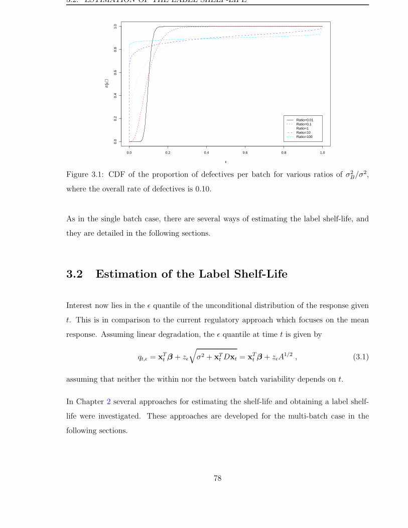
3.2. ESTIMATION OF THE LABEL SHELF-LIFE
0.0 0.2 0.4 0.6 0.8 1.0
0.0
0.2
0.4
0.6
0.8
1.0
ε
F(ε
)
Ratio=0.01Ratio=0.1Ratio=1Ratio=10Ratio=100
Figure 3.1: CDF of the proportion of defectives per batch for various ratios of σ2B/σ
2,
where the overall rate of defectives is 0.10.
As in the single batch case, there are several ways of estimating the label shelf-life, and
they are detailed in the following sections.
3.2 Estimation of the Label Shelf-Life
Interest now lies in the ε quantile of the unconditional distribution of the response given
t. This is in comparison to the current regulatory approach which focuses on the mean
response. Assuming linear degradation, the ε quantile at time t is given by
qt,ε = xTt β + zε
√
σ2 + xTt Dxt = xT
t β + zεA1/2 , (3.1)
assuming that neither the within nor the between batch variability depends on t.
In Chapter 2 several approaches for estimating the shelf-life and obtaining a label shelf-
life were investigated. These approaches are developed for the multi-batch case in the
following sections.
78
3.2. ESTIMATION OF THE LABEL SHELF-LIFE
3.2.1 Normal Approximation
An estimate for qt,ε can be obtained by replacing β, σ2 and D in (3.1) with appropri-
ate estimates. As in Chapter 2, it will be assumed that this estimate is approximately
normally distributed, and confidence bounds will be calculated.
The ordinary least squares estimates of bj are obtained by treating batches as fixed, such
that the estimates are given by bj = (XTj Xj)
−1XTj yj , with distribution bj ∼ N(β,Ωj),
where Ωj = D + σ2(XTj Xj)
−1. Carter and Yang (1986) take a weighted average of these
bj as an estimate of β, that is,
β(γ) = Ω
(
1
k
k∑
j=1
Ω−1j bj
)
(3.2)
where γ is the 1 + p (1+p)2
column vector containing σ2 and the upper-diagonal elements
of D and Ω is the harmonic mean of the Ωj , that is,
Ω =
(
1
k
k∑
j=1
Ω−1j
)−1
.
It is straight forward to show that (3.2) is equal to the generalised least squares estimator
of β under (1.7), given by
β(γ) =(
XTΣ−1X)−1(
XTΣ−1y)
=
(
k∑
j=1
XTj Σ−1
j Xj
)−1( k∑
j=1
XjΣ−1j yj
)
,
by noting that
Σ−1j =
1
σ2
[
Ij −Xj
(
σ2D−1 +XTj Xj
)−1XT
j
]
Ω−1j =
1
σ2XT
j
[
Ij −Xj
(
σ2D−1 +XTj Xj
)−1XT
j
]
Xj ,
and hence XTj Σ−1
j Xj(XTj Xj)
−1XTj = XT
j Σ−1j and Ω−1
j = XTj Σ−1
j Xj . The distribution of
the generalised least squares estimate is given by
β(γ) ∼ N(
β, 1kΩ)
.
79

3.2. ESTIMATION OF THE LABEL SHELF-LIFE
An estimate of σ2 is obtained by pooling the residuals across all batches, that is,
s2 =1
ν
k∑
j=1
(yj −Xjbj)T (yj −Xjbj) ,
where ν = N − kp . The distribution of νs2/σ2 is χ2ν .
An estimate of Ω is given by
(k − 1) Ω =
k∑
j=1
(bi − b.)(bi − b.)T ,
where b. = 1k
∑kj=1 bj. The distribution of (k − 1) Ω is Wishart with k − 1 degrees of
freedom, that is,
(k − 1) Ω ∼W (k − 1,Ω) .
The Wishart distribution is a multivariate generalization of the χ2 distribution and it
should be noted that for any p× 1 vector x
(k − 1)xT Ωx
xT Ωx∼ χ2
k−1 .
An estimate of D can then be obtained using
D = Ω − s2
k
k∑
j=1
(XTj Xj)
−1 , (3.3)
which can potentially be non-positive definite. In such a case it may be reasonable to use
the estimator suggested by Carter and Yang (1986).
A general form of the estimate of (3.1) can then be written as
qt,ε = xTt β(γ) +
√
δ2W s
2G+ δ2BxT
t Ωxt ,
where G = 1 − xTt
[
1k
∑kj=1(X
Tj Xj)
−1]
xt, and possible choices for δ2W and δ2
B include:
1. δ2W = δ2
B = z2ε ,
2.√
δ2W s
2G+ δ2BxT
t Ωxt is maximum likelihood for zεA1/2, and
3.√
δ2W s
2G+ δ2BxT
t Ωxt is unbiased for zεA1/2.
80
3.2. ESTIMATION OF THE LABEL SHELF-LIFE
As before, the performance of the normal approximation relies on the choice of δ2W and
δ2B and the closeness to normality of xT
t β(γ) and√
δ2W s
2G+ δ2BxT
t Ωxt. Note that s2 and
Ω are the maximum likelihood estimates for σ2 and Ω, which can easily be obtained from
the joint likelihood of s2 and Ω. It then follows that (1) and (2) above are identical.
Satterthwaite (1946) suggested a method of determining an approximate distribution of
a linear combination of mean squares, like that under the square root. The Satterthwaite
approximation states that when m2 is a linear combination of mean squares, that is,
m2 =∑
cim2i , where the ci are known constants and m2
i is estimated on fi degrees of
freedom, then m2 is distributed approximately as σ2mχ
2f/f , where E [m2 ] = σ2
m and the
approximate degrees of freedom, f , are given by
f =
(
∑
cim2i
)2
∑ (cim2
i )2
fi
. (3.4)
Consequently,δ2W s
2G+ δ2BxT
t Ωxt
δ2Wσ
2G+ δ2BxT
t Ωxt
∼χ2
f
f,
where the Satterthwaite degrees of freedom are given by
f =
[
δ2W s
2G + δ2BxT
t Ωxt
]2
[
δ2
W s2G]2
∑kj=1
(nj−2)+
[
δ2
BxTt Ωxt
]2
k−1
.
As a result, the expected value and variance of the square root are given by
E
[
√
δ2W s
2G+ δ2BxT
t Ω xt
]
= Cf
√
δ2Wσ
2G+ δ2BxT
t Ωxt
and
Var
[
√
δ2W s
2G+ δ2BxT
t Ωxt
]
=(
1 − C2f
)
[
δ2Wσ
2G+ δ2BxT
t Ωxt
]
.
Hence, the mean and variance of qt,ε are given by
E [ qt,ε ] = xTt β + Cf
√
δ2W s
2G+ δ2BxT
t Ωxt
Var [ qt,ε ] = 1kxT
t Ωxt +(
1 − C2f
)
[
δ2Wσ
2G + δ2BxT
t Ωxt
]
.
81
3.2. ESTIMATION OF THE LABEL SHELF-LIFE
From the expected value it follows that the three choices for δ2W and δ2
B are
Estimate (1) and (2): δ2W = δ2
B =z2ε (3.5)
Estimate (3): δ2W = δ2
B =z2
ε
C2ν
, (3.6)
and an estimate of the variance can be obtained by substituting s2 and Ω for σ2 and Ω
in the variance for qt,ε. Thus, the estimated shelf-life is given by
τε = inf t : qt,ε ≤ κ ,
and the label shelf-life is the time at which the 100(1 − α)% lower confidence bound for
qt,ε intersects the specification limit, that is,
τε,L(α) = inf
t : qt,ε + tα,f
√
1kxT
t Ωxt +(
1 − C2f
)
[
δ2W s
2G+ δ2BxT
t Ωxt
]
≤ κ
. (3.7)
Notice that (3.7) must be solved iteratively for t, as t is used under the square root sign as
well as in the calculation of tα,f . Also, zα could be used instead of tα,f , but the simulations
in Chapter 2 have shown that the normal quantile performed worse than the appropriate
quantile from the t-distribution, especially for small samples.
3.2.2 Various Profile Likelihood Based Approaches
This section details methods analogous to those in 2.2.2 and 2.2.3 for the situation when
multiple batches are analysed together.
The label shelf-life τε,L(α) is again the smallest time τ for which the null hypothesis
H0 : β0 + β1τ + zε
√
σ + xTt D xt = κ (3.8)
is retained on a one-sided 100α% level test. Both κ and zε are known constants, and
thus the likelihood can be reformulated as a function of the parameters (β1, σ2, D, τ), by
eliminating β0. Hypotheses about τ can then be tested using the profile likelihood, which
is obtained by maximizing the likelihood over (β1, σ,D) for given values of τ .
82
3.2. ESTIMATION OF THE LABEL SHELF-LIFE
The Basic Profile Likelihood
The log-likelihood based on (1.7) is given by
L(β, σ,D;y) = −1
2log |Σ| − 1
2
(
y − Xβ)T
Σ−1(
y − Xβ)
= −1
2
k∑
j=1
log |Σj| −1
2
k∑
j=1
rTj Σ−1
j rj , (3.9)
where rj = yj −Xjβ.
The maximum likelihood estimates of the parameters are found by differentiating (3.9)
with respect to β, σ2 and the elements dl of D, and equating the derivatives to zero. That
is,
∂L
∂β=
k∑
j=1
XTj Σ−1
j rj
∂L
∂σ2= −1
2
k∑
j=1
tr
Σ−1j
+1
2
k∑
j=1
rTj Σ−2
j rj
∂L
∂dl= −1
2
k∑
j=1
tr
Σ−1j Xj
∂D
∂dlXT
j
+1
2
k∑
j=1
rTj Σ−1
j Xj∂D
∂dlXT
j Σ−1j rj ,
which do not have explicit solutions. However, Fisher scoring can be employed to find
the maximum likelihood estimates.
The elements of the observed information matrix Io are given by
Io(β,β) =
k∑
j=1
XTj Σ−1
j Xj
Io(β, σ2) =
k∑
j=1
XTj Σ−2
j rj
Io(β, dl) =
k∑
j=1
XTj Σ−1
j Xj∂D
∂dlXT
j Σ−1j rj
Io(σ2, σ2) = −1
2
k∑
j=1
tr
Σ−2j
+
k∑
j=1
rTj Σ−3
j rj
Io(σ2, dl) = −1
2
k∑
j=1
tr
Σ−1j Xj
∂D
∂dlXT
j Σ−1j
+
k∑
j=1
rTj Σ−2
j Xj∂D
∂dlXT
j Σ−1j rj
83
3.2. ESTIMATION OF THE LABEL SHELF-LIFE
Io(dl, dm) = −1
2
k∑
j=1
tr
Σ−1j Xj
∂D
∂dlXT
j Σ−1j Xj
∂D
∂dmXT
j
+k∑
j=1
rTj Σ−1
j Xj∂D
∂dlXT
j Σ−1j Xj
∂D
∂dmXT
j Σ−1j rj .
Hence, the elements of the expected information matrix are
Ie(β,β) =k∑
j=1
XTj Σ−1
j Xj
Ie(β, σ2) = 0
Ie(β, dl) = 0
Ie(σ2, σ2) =
1
2
k∑
j=1
tr
Σ−2j
Ie(σ2, dl) =
1
2
k∑
j=1
tr
Σ−1j XT
j
∂D
∂dlXT
j Σ−1j
Ie(dl, dm) =1
2
k∑
j=1
tr
Σ−1j XT
j
∂D
∂dlXT
j Σ−1j XT
j
∂D
∂dmXT
j
.
Denoting the maximum likelihood estimate of β, σ2 and D by β, σ2 and D, respectively,
it is easy to find the maximum likelihood estimate of τε, that is,
τε = inf
t : xTt β + zε
√
σ2 + xTt Dxt ≤ κ
.
The profile likelihood of τε is obtained by eliminating β0 in (3.9) using the null hypothesis
(3.8), and subscripting the parameters with τε to indicate their dependence on τε, that is,
L(τε;y) = −1
2
k∑
j=1
log |Σj,τε| −1
2
k∑
j=1
r∗Tj Σ−1j,τεr∗j ,
where
r∗j = y∗j −X∗
j β1,τε + 1jzεA1/2 ,
and 1j is a Nj × 1 vector of 1’s, y∗j = yj − 1jκ, X
∗j = X(j) − 1jτε, X(j) is the model
matrix Xj without the column corresponding to β0, and A1/2 =√
σ2τε
+ xTτεDτεxτε , where
xτε = x(τε).
84
3.2. ESTIMATION OF THE LABEL SHELF-LIFE
Differentiating the profile likelihood with respect to β1,τε , σ2τε
and dl,τε gives
∂L
∂β1,τε
=
k∑
j=1
X∗Tj Σ−1
j,τεr∗j
∂L
∂σ2τε
= −1
2
k∑
j=1
tr
Σ−1j,τε
+1
2
k∑
j=1
r∗Tj Σ−2j,τε
r∗j −zε
2A1/2
k∑
j=1
1Tj Σ−1
j,τεr∗j
∂L
∂dl,τε
= −1
2
k∑
j=1
tr
Σ−1j,τεXj
∂Dτε
∂dlXT
j
+1
2
k∑
j=1
r∗Tj Σ−1j,τεXj
∂Dτε
∂dlXT
j Σ−1j,τε
r∗j
− zε
2A1/2
(
xTτε
∂Dτε
∂dl,τε
xτε
)
k∑
j=1
1Tj Σ−1
j,τεr∗j .
The elements of the observed information matrix are consequently given by
Io(β1,τε , β1,τε) =k∑
j=1
X∗Tj Σ−1
j,τεX∗
j
Io(β1,τε, σ2τε
) =k∑
j=1
X∗Tj Σ−2
j,τεr∗j −
zε
2A1/2
k∑
j=1
X∗Tj Σ−1
j,τε1j
Io(β1,τε, dl,τε) =k∑
j=1
X∗Tj Σ−1
j,τεXj
∂Dτε
∂dl,τε
XTj Σ−1
j,τεr∗j
− zε
2A1/2
(
xTτε
∂Dτε
∂dl,τε
xτε
)
k∑
j=1
X∗Tj Σ−1
j,τε1j
Io(σ2τε, σ2
τε) = −1
2
k∑
j=1
tr
Σ−2j,τε
+k∑
j=1
r∗Tj Σ−3j,τε
r∗j +z2
ε
4A
k∑
j=1
1Tj Σ−1
j,τε1j
− zε
A1/2
k∑
j=1
1Tj Σ−2
j,τεr∗j −
z2ε
4A3/2
k∑
j=1
1Tj Σ−1
j,τεr∗j
Io(σ2τε, dl,τε) = −1
2
k∑
j=1
tr
Σ−1j,τεXj
∂Dτε
∂dl,τε
XTj Σ−1
j,τε
+k∑
j=1
r∗Tj Σ−2j,τεXj
∂Dτε
∂dl,τε
XTj Σ−1
j,τεr∗j
+z2
ε
4A
(
xTτε
∂Dτε
∂dl,τε
xτε
)
k∑
j=1
1Tj Σ−1
j,τε1j −
zε
A1/2
(
xTτε
∂Dτε
∂dl,τε
xτε
)
k∑
j=1
1Tj Σ−2
j,τεr∗j
− z2ε
4A3/2
(
xTτε
∂Dτε
∂dl,τε
xτε
)
k∑
j=1
1Tj Σ−1
j,τεr∗j
Io(dl,τε, dm,τε) = −1
2
k∑
j=1
tr
Σ−1j,τεXj
∂Dτε
∂dm,τε
XTj Σ−1
j,τεXj
∂Dτε
∂dl,τε
XTj
85
3.2. ESTIMATION OF THE LABEL SHELF-LIFE
+k∑
j=1
r∗Tj Σ−1j,τεXj
∂Dτε
∂dm,τε
XTj Σ−1
j,τεXj
∂Dτε
∂dl,τε
XTj Σ−1
j,τεr∗j
+z2
ε
4A
(
xTτε
∂Dτε
∂dm,τε
xτε
)(
xTτε
∂Dτε
∂dl,τε
xτε
)
k∑
j=1
1Tj Σ−1
j,τε1j
− zε
2A1/2
(
xTτε
∂Dτε
∂dl,τε
xτε
)
k∑
j=1
1Tj Σ−2
j,τεr∗j
− zε
2A1/2
(
xTτε
∂Dτε
∂dm,τε
xτε
)
k∑
j=1
1Tj Σ−2
j,τεr∗j
− z2ε
4A3/2
(
xTτε
∂Dτε
∂dm,τε
xτε
)(
xTτε
∂Dτε
∂dl,τε
xτε
)
k∑
j=1
1Tj Σ−1
j,τεr∗j .
Taking expectations gives the elements of the expected information matrix,
Ie(β1,τε , β1,τε) =k∑
j=1
X∗Tj Σ−1
j,τεX∗
j
Ie(β1,τε , σ2τε
) = − zε
2A1/2
k∑
j=1
X∗Tj Σ−1
j,τε1j
Ie(β1,τε , dl,τε) = − zε
2A1/2
(
xTτε
∂Dτε
∂dl,τε
xτε
)
k∑
j=1
X∗Tj Σ−1
j,τε1j
Ie(σ2τε, σ2
τε) =
1
2
k∑
j=1
tr
Σ−2j,τε
+z2
ε
4A
k∑
j=1
1Tj Σ−1
j,τε1j
Ie(σ2τε, dl,τε) =
1
2
k∑
j=1
tr
Σ−1j,τεXj
∂Dτε
∂dl,τε
XTj Σ−1
j,τε
+z2
ε
4A
(
xTτε
∂Dτε
∂dl,τε
xτε
)
k∑
j=1
1Tj Σ−1
j,τε1j
Ie(dl,τε, dm,τε) = +1
2
k∑
j=1
tr
Σ−1j,τεXj
∂Dτε
∂dm,τε
XTj Σ−1
j,τεXj
∂Dτε
∂dl,τε
XTj
+z2
ε
4A
(
xTτε
∂Dτε
∂dm,τε
xτε
)(
xTτε
∂Dτε
∂dl,τε
xτε
)
k∑
j=1
1Tj Σ−1
j,τε1j .
Consequently, Fisher scoring can be implemented to obtain estimates β1,τε, σ2τε
and Dτε . As
before, the likelihood ratio test can be used to obtain the label shelf-life from a 100(1−α)%
lower confidence bound for τε. Let L(τε;y) be the likelihood evaluated at the maximum
likelihood estimates and let L(τε;y) be the likelihood evaluated for a given value of τε.
86
3.2. ESTIMATION OF THE LABEL SHELF-LIFE
Then, asymptotically, the generalised likelihood ratio statistic is given by
w(τ) = 2(
L(τε;y) − L(τε;y))
,
which is distributed approximately χ21 when (3.8) is true. Consequently, the label shelf-life
is given by
τε,L(α) = inf
t : (t ≤ τε) & (w(t) ≤ χ21,1−2α)
. (3.10)
The Truncated Modified Profile Likelihood (TMPL) Approach
Unlike in the single batch case of Chapter 2 parameter estimates cannot be obtained
analytically. Consequently, the Jacobian term used in the modified profile likelihood
(2.22) cannot be calculated. Nevertheless, it is possible to calculate the observed and
expected truncated modified profile likelihoods.
The observed modified profile log-likelihood for τε is given by
Lom
(
τε;y)
= L(
τε;y)
− 1
2log∣
∣
∣Io(β1,τε, σ
2τε, Dτε)
∣
∣
∣− log
∣
∣
∣
∣
∣
∂(β1,τε , σ2τε, Dτε)
∂(β1, σ2, D)
∣
∣
∣
∣
∣
.
Consequently, the observed truncated modified profile likelihood is obtained by ignoring
the Jacobian term, that is,
Lot
(
τε;y)
= L(
τε;y)
+1
2log∣
∣
∣Io(β1,τε , σ
2τε, Dτε)
∣
∣
∣.
The generalised likelihood ratio statistic is then given by
wt(τ) = 2(
Lot (τε;y) − Lo
t (τε;y))
,
which is distributed approximately χ21 when (3.8) is true. Consequently, the label shelf-life
is given by
τε,L(α) = inf
t : (t ≤ τε) & (wt(t) ≤ χ21,1−2α)
. (3.11)
Similarly to Chapter 2, the expected information matrix can be used, resulting in Lot
being replaced by Let .
87
3.2. ESTIMATION OF THE LABEL SHELF-LIFE
The Conditional Profile Likelihood Approach
The conditional profile likelihood (2.24) depends on the orthogonality of the parameters
to ψ = τε. Consequently, the original parameters φT = (β1,τε, σ2τε, d1,τε, d2,τε, d3,τε) must be
transformed to give a new set of parameters λT = (λ1, . . . , λ5), which are orthogonal to
ψ = τε. This is done by solving the differential equations
Ie(φ,φ)∂φ
∂ψ= −Ie(φ, ψ) ,
Note that the information matrix Ie(φ,φ) is a 5×5 matrix, which makes the inversion, and
consequent integration, analytically intractable. Hence, the conditional profile likelihood
does not offer a usable alternative in the multi-batch case.
3.2.3 Constrained Profile Likelihood Based Approaches
It has been shown in Section 2.2.3 that the constrained profile likelihood, based on the
Powell-Hestenes approach advocated by Osborne (2000), can be used in place of the
basic profile likelihood approach. As expected, the results were identical numerically. In
addition, an approximation to the modified profile likelihood was obtained even though
the Jacobian term could not be approximated. This section will detail both methods
when applied to the batch case.
The objective function, based on (3.9), is given by
H(βτε, σ2, D, τε;y) =
1
N
[
−L(θτε)]
+ ω[
g(θτε ; τε) + ψ]2, (3.12)
where θTτε
= (βTτε, σ2
τε, d1,τε, d2,τε, d3,τε) and
g(θτε ; τε) = xTτεβτε
+ zεA1/2τε
− κ , (3.13)
where A1/2τε =
√
σ2τε
+ xTτεDτεxτε . The aim is to minimise the objective function subject to
g(θτε ; τε) = 0. This can again be achieved with the help of Fisher Scoring.
88
3.2. ESTIMATION OF THE LABEL SHELF-LIFE
Letting rj = yj −Xjβτε, the elements of the score vector are given by
∂H
∂βτε
=1
N
[
−k∑
j=1
XTj Σ−1
j,τεrj
]
+ 2ω[
g(θτε ; τε) + ψ]
xτε
∂H
∂σ2τε
=1
2N
[
k∑
j=1
tr
Σ−1j,τε
−k∑
j=1
rTj Σ−2
j,τεrj
]
+ωzε
A1/2τε
[
g(θτε ; τε) + ψ]
∂H
∂dl,τε
=1
2N
[
k∑
j=1
tr
Σ−1j,τεXj
∂Dτε
∂dl,τε
XTj
−k∑
j=1
rTj Σ−1
j,τεXj
∂Dτε
∂dl,τε
XTj Σ−1
j rj
]
+ωzε
A1/2τε
(
xTτε
∂Dτε
∂dl,τε
xτε
)
[
g(θτε ; τε) + ψ]
,
Note that the unconstrained estimates can be obtained by ignoring the terms involving
the constraint, which is equivalent to setting ω = 0. It is easy to see that this yields the
same maximum likelihood estimates that were obtained in Section 3.2.2.
The elements of the Powell-Hestenes equivalents of the observed information matrix, ig-
noring terms involving the second derivative of g(θτε ; τε), are then given by
Io′(βτε
,βτε) =
1
N
[
k∑
j=1
XTj Σ−1
j,τεXj
]
+ 2ω xτεxTτε
Io′(βτε
, σ2τε
) =1
N
[
k∑
j=1
XTj Σ−2
j,τεrj
]
+ωzε
A1/2τε
xτε
Io′(βτε
, dl,τε) =1
N
[
k∑
j=1
XTj Σ−1
j,τεXj
∂Dτε
∂dl,τε
XTj Σ−1
j,τεrj
]
+ωzε
A1/2τε
(
xTτε
∂Dτε
∂dl,τε
xτε
)
xτε
Io′(σ2
τε, σ2
τε) =
1
N
[
−1
2
k∑
j=1
tr(
Σ−2j,τε
)
+k∑
j=1
rTj Σ−3
j,τεrj
]
+ωz2
ε
2Aτε
Io′(σ2
τε, dl,τε) =
1
N
[
−1
2
k∑
j=1
tr
(
Σ−1j,τεXj
∂Dτε
∂dl,τε
XTj Σ−1
j,τε
)
+k∑
j=1
rTj Σ−2
j,τεXj
∂Dτε
∂dl,τε
XTj Σ−1
j,τεrj
]
+ωz2
ε
2Aτε
(
xTτε
∂Dτε
∂dl,τε
xτε
)
Io′(dl,τε, dm,τε) =
1
N
[
−1
2
k∑
j=1
tr
(
Σ−1j,τεXj
∂Dτε
∂dm,τε
XTj Σ−1
j,τεXj
∂Dτε
∂dl,τε
XTj
)
+
k∑
j=1
rTj Σ−1
j,τεXj
∂Dτε
∂dm,τε
XTj Σ−1
j,τεXj
∂Dτε
∂dl,τε
XTj Σ−1
j,τεrj
]
+ωz2
ε
2Aτε
(
xTτε
∂Dτε
∂dm,τε
xτε
)(
xTτε
∂Dτε
∂dl,τε
xτε
)
.
89
3.2. ESTIMATION OF THE LABEL SHELF-LIFE
Taking expectations gives the elements of the equivalent versions of the expected infor-
mation matrix
Ie′(βτε
,βτε) =
1
N
[
k∑
j=1
XTj Σ−1
j,τεXj
]
+ 2ω xτεxTτε
Ie′(βτε
, σ2τε
) = 0 +ωzε
A1/2τε
xτε
Ie′(βτε
, dl,τε) = 0 +ωzε
A1/2τε
(
xTτε
∂Dτε
∂dl,τε
xτε
)
xτε
Ie′(σ2
τε, σ2
τε) =
1
2N
k∑
j=1
tr(
Σ−2j,τε
)
+ωz2
ε
2Aτε
Ie′(σ2
τε, dl,τε) =
1
2N
k∑
j=1
tr
(
Σ−1j,τεXj
∂Dτε
∂dl,τε
XTj Σ−1
j,τε
)
+ωz2
ε
2Aτε
(
xTτε
∂Dτε
∂dl,τε
xτε
)
Ie′(dl,τε, dm,τε) =
1
2N
k∑
j=1
tr
(
Σ−1j,τεXj
∂Dτε
∂dm,τε
XTj Σ−1
j,τεXj
∂Dτε
∂dl,τε
XTj
)
+ωz2
ε
2Aτε
(
xTτε
∂Dτε
∂dm,τε
xτε
)(
xTτε
∂Dτε
∂dl,τε
xτε
)
.
As before, Fisher scoring can now be used to obtain estimates βτε, σ2
τεand Dτε. As before,
the likelihood ratio test can be used to obtain the label shelf-life from the 100(1 − α)%
lower confidence bound for τε. Let L(τε;y) be the likelihood evaluated at the maximum
likelihood estimates and let L(τε;y) be the likelihood evaluated for a given value of τε.
Then, asymptotically, the generalised likelihood ratio statistic is given by
w(τ) = 2(
L(τε;y) − L(τε;y))
,
which is distributed approximately χ21 when (3.8) is true. Consequently, the label shelf-life
is given by
τε,L(α) = inf
t : (t ≤ τε) & (w(t) ≤ χ21,1−2α)
. (3.14)
The Modified Constrained Profile Likelihood
In Section 3.2.2 it was shown that a modified profile likelihood approach was not possible
when β1 was eliminated from the profile likelihood. Nevertheless, the truncated modified
profile likelihood provides a usable adjustment when the modified profile likelihood is
90
3.2. ESTIMATION OF THE LABEL SHELF-LIFE
not possible. In addition, an approximation to the truncated modified profile likelihood,
was developed in Section 2.2.3. This approach has performed well in the simulations of
Chapter 2 and this Section will detail its application in the multi-batch scenario.
The approximation detailed in Section 2.2.3 was very general in terms of the number of
parameters that are estimated. As such, the approximation can very easily be applied to
the multi-batch scenario, since (2.34) and (2.37) still apply here, with p = 6.
The derivative of the constraint (3.13) in the batch case gives
∂g(θτε , τε)
∂θTτε
=[
1 τεzε
2A1/2
τε
zε
2A1/2
τε
zετε
A1/2
τε
zετ2ε
2A1/2
τε
]
θτε= θ0,τε
,
where the obvious choice for θ0,τε is again the constrained maximum likelihood estimate
θτε , giving
C0 =[
1 τεzε
2A1/2
τε
zε
2A1/2
τε
zετε
A1/2
τε
zετ2ε
2A1/2
τε
]
.
The approximate modified profile likelihood is now given by
La(τε;y) = L(θτε;y) − 1
2log
[
det
C0Io(θτε)−1CT
0
[
det
C0CT0
]−1
det
Io(θτε)
]
from which τε can be estimated. The generalised likelihood ratio statistic is given by
wa(τε) = 2(
La(τε;y) − La(τε;y))
,
which is distributed approximately χ21 under (2.7). Consequently, the label shelf-life,
based on the 100(1 − α)% lower confidence bound, is given by
τε,L(α) = inf
t : (t ≤ τε) ∩ (wa(t) ≤ χ21,1−2α)
. (3.15)
3.2.4 Non-central t-distribution (NCT) Approach
In Section 2.2.4 an exact lower confidence bound for τε was found based on the distribution
of β. In the batch case, the distribution of β is given by
β ∼ N(
β, 1kΩ)
,
91
3.2. ESTIMATION OF THE LABEL SHELF-LIFE
as described in Section 3.2.1. The mean response at time t is then given by xTt β, with
distribution
xTt β ∼ N
(
xTt β, 1
kxT
t Ωxt
)
.
From (3.1) it follows that xTt β = qt,ε − zεA
1/2, and hence standardizing xTt β yields
(
xTt β − qt,ε + zεA
1/2)√k
√
xTt Ωxt
∼ N(0, 1) .
Alternatively, this can be written as
(
xTt β − qt,ε
)√k
√
xTt Ωxt
∼ N
−zεA1/2
√k
√
xTt Ωxt
, 1
. (3.16)
Note that A1/2 =√
σ2 + xTt D xt which does not equal
√
xTt Ωxt. This can easily be seen
from the case when all Xj are equal to X, say, in which case Ω = D + σ2(XTX)−1 and
xTt Ωxt = xT
t Dxt + σ2xTt (XTX)−1xt. Consequently, unlike Section 2.2.4, these elements
do not cancel from the mean of the normal distribution.
However, when between batch variability is large compared to within batch variability, or
more precisely, when xTt D xt is large compared to σ2, then A1/2 ≈
√
xTt Ωxt ≈
√
xTt D xt,
in which case(
xTt β − qt,ε
)√k
√
xTt Ωxt
∼ N
−zε
√k, 1
.
Consequently, replacing xTt Ωxt by its estimate xT
t Ωxt results in a non-central
t-distribution, that is,(
xTt β − qt,ε
)√k
√
xTt Ωxt
∼ t′(
k − 1, δ)
,
where δ = −zε
√k denotes the non-centrality parameter. The label shelf-life is given by
the intersection of the 100(1 − α)% lower confidence bound and the specification limit,
that is,
τε,L(α) = inf
t : xTt β +Qα
√
xTt Ωxt
k≤ κ
, (3.17)
where Qα = t′α(k − 1,−δ) is the lower α quantile of the non-central t-distribution with
k − 1 degrees of freedom and non-centrality parameter δ = −zε
√k. Note that this
approximation is what Shao and Chow (1994) rely on for their definition of shelf-life in
92
3.2. ESTIMATION OF THE LABEL SHELF-LIFE
the batch case. In fact, (3.17) is equivalent to the label shelf-life of Shao and Chow, with
the above derivation being alternative to that provided by Shao and Chow.
It should be noted that in the limiting case as k → ∞, the label shelf-life (3.17) becomes
τε,L(α) = inf
t : xTt β + zε
√
σ2xTt (XTX)−1xt + xT
t Dxt ≤ κ
,
since t′α(k−1,−δ) → (zα + zε
√k). Generally xt(X
TX)−1xt < 1, and hence it follows that
zε
√
σ2xTt (XTX)−1xt + xT
t Dxt ≤ zε
√
σ2 + xTt Dxt .
Consequently, using this method will result in a label shelf-life that is greater than the true
shelf-life. In addition, since (XTX)−1 → 0 as N → ∞ it follows that this approximation
gets worse as the sample size increases.
However, Shao and Chow (1994) use the following definition of the true shelf-life
τ ∗ε = inf
t : xTt β + zε
√
xTt Dxt ≤ κ
. (3.18)
Thus, Shao and Chow’s label shelf-life is the 100(1−α)% lower confidence bound for the
time at which the ε quantile of the distribution of xTt bj intersects the specification limit.
In this case, (3.17) will be conservative, as was observed by Shao and Chow.
When σ2 is not small compared to xTt D xt then an approximate answer may be obtained
by replacing σ2, D and Ω in the mean of the distribution in (3.16) by their respective
estimates and considering the mean as fixed. In this case, (3.17) still holds, but the
non-centrality parameter takes the form
δ = −zε
√
k(s2 + xTt D xt)
xTt Ωxt
. (3.19)
Even though these two NCT approaches are approximate only, they will be further eval-
uated in Section 3.3.
93
3.3. SIMULATION RESULTS
3.3 Simulation Results
As in the single batch case, a simulation study is used to evaluate the approaches proposed
in this chapter. These simulations were again performed with the help of the software
R (Ihaka and Gentleman, 1996). Compared to the single batch case, simulations in the
batch case are very much more computationally intensive.
The simulations were structured as follows. A random sample of batch effects of size
k = 3, 5, 10 and 20 was drawn from the bj ∼ N(β, D). The mean was chosen to be
βT = (100,−0.3), while
D =
1 d2
d2 0.003
,
for d2 = −0.03, 0 or 0.03. Then a random sample of responses of size r = 1, 2 and 5 was
drawn from each conditional distribution Yij|bj ∼ N(xTi bj , σ
2), where xi = c(1, xi), the
xi are as before 0, 3, 6, 9, 12, 18, 24 and 36 months, and σ = 0.5, 1 and 2. The total
number of observations used in the analysis is then N = knr, where n denotes the number
of times (n = 8). Note that, without loss of generality, the same times xi were used for
each batch. This was done for two reasons: firstly, the coding and analysis are easier
and less time consuming, and secondly, these times are those suggested by the regulatory
authorities (even though other times may be more appropriate, c.f. Section 1.1).
Assuming that the specification limit was again set at κ = 90 and that ε = 0.01, the true
shelf-life (in months) is given by the smaller root to qt,ε = κ. For each combination of
k, r, d2 and σ, 1000 simulations were performed and for each simulation the data were
analysed using each method, using a 95% lower confidence bound (α = 0.05). For each
method the proportion of label shelf-lives that were smaller than the true shelf-life was
calculated. These proportions can be found in Tables 3.1–3.9. Approximate confidence
bounds for the true proportions can again be obtained using the normal approximation
to the binomial described in Section 2.3.
The simulation results are summarised in the following tables and graphs. The coverage
probabilities are displayed in Tables 3.1–3.9 and Figure 3.2; the bias is summarised in
94
3.3. SIMULATION RESULTS
Tables 3.10–3.18 and Figure 3.3; and the mean square error is summarised in Tables 3.19–
3.27 and Figure 3.4. Again, the “bias” is not a bias in the true sense, but serves as an
indicator of how conservative a particular method is (c.f. Section 2.3). As in Chapter 2
the methods are abbreviated, and the key is as follows.
• z.t and U.t denote the normal approximation approaches (3.7), using δ given in (3.5)
and (3.6), respectively. The confidence bounds are calculated using t distribution.
• CPL denotes the constrained profile likelihood approach (3.14)
• TMCPL denotes the truncated modified constrained profile likelihood approach
(3.15).
• NCT1 and NCT2 denote the non-central t-distribution approach (3.17), using the
unmodified δ and the modified δ given in (3.19).
Similar to Chapter 2, these tables can be summarized further by fitting appropriate mod-
els. In the case of the coverage probability it can be seen from Tables 3.1-3.9 and Figure 3.2
that the coverage probability does not appear to depend appreciably on the number of
assays per batch. A similar full model for the coverage probability to that of Chapter 2
was fitted here. However, the full model involved 1/k, 1/√N , σ∗ and d2 as explanatory
variables. Again, standard model reduction was conducted by testing higher order terms
in turn and observing marginality (assuming a significance level of 1%). Table 3.28 gives
the parameter estimates for all significant effects (interactions that were not significant
under any method are omitted from the table). Even though only one value of β1 was
used in these simulations, it is not unreasonable to expect that the methods behave in a
similar way to those in Chapter 2.
A similar modeling approach to that in Chapter 2 was also undertaken for the bias,
and the results of the significant parameter estimates (at the 1% significance level) are
presented in Table 3.29. The results are discussed in Section 3.4.
95
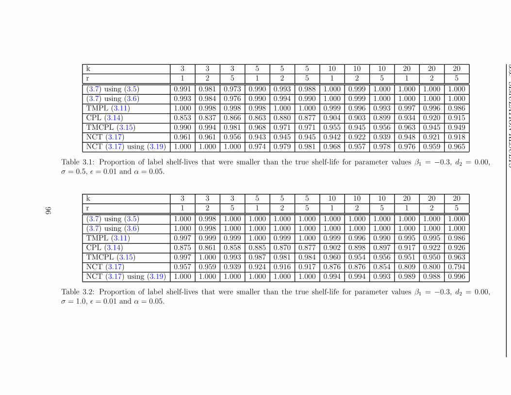
3.3
.SIM
ULA
TIO
NR
ESU
LT
S
k 3 3 3 5 5 5 10 10 10 20 20 20r 1 2 5 1 2 5 1 2 5 1 2 5
(3.7) using (3.5) 0.991 0.981 0.973 0.990 0.993 0.988 1.000 0.999 1.000 1.000 1.000 1.000(3.7) using (3.6) 0.993 0.984 0.976 0.990 0.994 0.990 1.000 0.999 1.000 1.000 1.000 1.000TMPL (3.11) 1.000 0.998 0.998 0.998 1.000 1.000 0.999 0.996 0.993 0.997 0.996 0.986CPL (3.14) 0.853 0.837 0.866 0.863 0.880 0.877 0.904 0.903 0.899 0.934 0.920 0.915TMCPL (3.15) 0.990 0.994 0.981 0.968 0.971 0.971 0.955 0.945 0.956 0.963 0.945 0.949NCT (3.17) 0.961 0.961 0.956 0.943 0.945 0.945 0.942 0.922 0.939 0.948 0.921 0.918NCT (3.17) using (3.19) 1.000 1.000 1.000 0.974 0.979 0.981 0.968 0.957 0.978 0.976 0.959 0.965
Table 3.1: Proportion of label shelf-lives that were smaller than the true shelf-life for parameter values β1 = −0.3, d2 = 0.00,σ = 0.5, ε = 0.01 and α = 0.05.
k 3 3 3 5 5 5 10 10 10 20 20 20r 1 2 5 1 2 5 1 2 5 1 2 5
(3.7) using (3.5) 1.000 0.998 1.000 1.000 1.000 1.000 1.000 1.000 1.000 1.000 1.000 1.000(3.7) using (3.6) 1.000 0.998 1.000 1.000 1.000 1.000 1.000 1.000 1.000 1.000 1.000 1.000TMPL (3.11) 0.997 0.999 0.999 1.000 0.999 1.000 0.999 0.996 0.990 0.995 0.995 0.986CPL (3.14) 0.875 0.861 0.858 0.885 0.870 0.877 0.902 0.898 0.897 0.917 0.922 0.926TMCPL (3.15) 0.997 1.000 0.993 0.987 0.981 0.984 0.960 0.954 0.956 0.951 0.950 0.963NCT (3.17) 0.957 0.959 0.939 0.924 0.916 0.917 0.876 0.876 0.854 0.809 0.800 0.794NCT (3.17) using (3.19) 1.000 1.000 1.000 1.000 1.000 1.000 0.994 0.994 0.993 0.989 0.988 0.996
Table 3.2: Proportion of label shelf-lives that were smaller than the true shelf-life for parameter values β1 = −0.3, d2 = 0.00,σ = 1.0, ε = 0.01 and α = 0.05.
96

3.3
.SIM
ULA
TIO
NR
ESU
LT
S
k 3 3 3 5 5 5 10 10 10 20 20 20r 1 2 5 1 2 5 1 2 5 1 2 5
(3.7) using (3.5) 1.000 1.000 1.000 1.000 1.000 1.000 1.000 1.000 1.000 1.000 1.000 1.000(3.7) using (3.6) 1.000 1.000 1.000 1.000 1.000 1.000 1.000 1.000 1.000 1.000 1.000 1.000TMPL (3.11) 1.000 1.000 1.000 1.000 1.000 1.000 0.989 0.986 0.991 0.980 0.974 0.979CPL (3.14) 0.914 0.897 0.865 0.901 0.891 0.893 0.911 0.910 0.927 0.918 0.924 0.933TMCPL (3.15) 0.987 0.998 0.999 0.985 0.996 0.994 0.958 0.961 0.971 0.948 0.954 0.953NCT (3.17) 0.949 0.919 0.901 0.782 0.734 0.703 0.528 0.405 0.364 0.169 0.095 0.065NCT (3.17) using (3.19) 1.000 1.000 1.000 1.000 1.000 1.000 1.000 1.000 1.000 0.999 1.000 1.000
Table 3.3: Proportion of label shelf-lives that were smaller than the true shelf-life for parameter values β1 = −0.3, d2 = 0.00,σ = 2.0, ε = 0.01 and α = 0.05.
k 3 3 3 5 5 5 10 10 10 20 20 20r 1 2 5 1 2 5 1 2 5 1 2 5
(3.7) using (3.5) 0.978 0.975 0.963 0.987 0.987 0.986 0.999 0.999 0.999 1.000 1.000 1.000(3.7) using (3.6) 0.983 0.979 0.968 0.988 0.988 0.989 1.000 0.999 0.999 1.000 1.000 1.000TMPL (3.11) 0.992 0.996 1.000 0.998 1.000 0.999 0.999 0.999 0.987 0.990 0.972 0.965CPL (3.14) 0.798 0.813 0.817 0.866 0.854 0.839 0.894 0.907 0.878 0.916 0.911 0.924TMCPL (3.15) 0.987 0.982 0.968 0.964 0.951 0.945 0.948 0.960 0.938 0.953 0.944 0.951NCT (3.17) 0.957 0.952 0.941 0.951 0.941 0.936 0.945 0.954 0.932 0.935 0.928 0.941NCT (3.17) using (3.19) 0.991 0.994 0.998 0.970 0.971 0.971 0.961 0.972 0.959 0.967 0.957 0.970
Table 3.4: Proportion of label shelf-lives that were smaller than the true shelf-life for parameter values β1 = −0.3, d2 = 0.03,σ = 0.5, ε = 0.01 and α = 0.05.
97
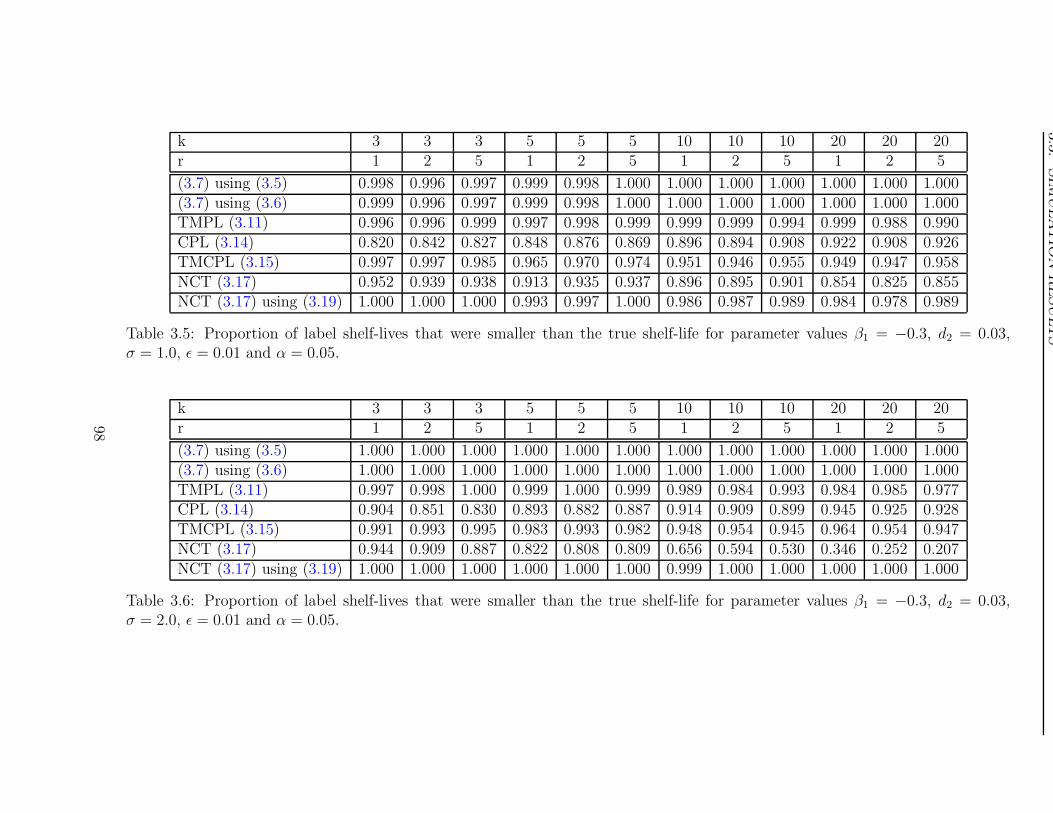
3.3
.SIM
ULA
TIO
NR
ESU
LT
S
k 3 3 3 5 5 5 10 10 10 20 20 20r 1 2 5 1 2 5 1 2 5 1 2 5
(3.7) using (3.5) 0.998 0.996 0.997 0.999 0.998 1.000 1.000 1.000 1.000 1.000 1.000 1.000(3.7) using (3.6) 0.999 0.996 0.997 0.999 0.998 1.000 1.000 1.000 1.000 1.000 1.000 1.000TMPL (3.11) 0.996 0.996 0.999 0.997 0.998 0.999 0.999 0.999 0.994 0.999 0.988 0.990CPL (3.14) 0.820 0.842 0.827 0.848 0.876 0.869 0.896 0.894 0.908 0.922 0.908 0.926TMCPL (3.15) 0.997 0.997 0.985 0.965 0.970 0.974 0.951 0.946 0.955 0.949 0.947 0.958NCT (3.17) 0.952 0.939 0.938 0.913 0.935 0.937 0.896 0.895 0.901 0.854 0.825 0.855NCT (3.17) using (3.19) 1.000 1.000 1.000 0.993 0.997 1.000 0.986 0.987 0.989 0.984 0.978 0.989
Table 3.5: Proportion of label shelf-lives that were smaller than the true shelf-life for parameter values β1 = −0.3, d2 = 0.03,σ = 1.0, ε = 0.01 and α = 0.05.
k 3 3 3 5 5 5 10 10 10 20 20 20r 1 2 5 1 2 5 1 2 5 1 2 5
(3.7) using (3.5) 1.000 1.000 1.000 1.000 1.000 1.000 1.000 1.000 1.000 1.000 1.000 1.000(3.7) using (3.6) 1.000 1.000 1.000 1.000 1.000 1.000 1.000 1.000 1.000 1.000 1.000 1.000TMPL (3.11) 0.997 0.998 1.000 0.999 1.000 0.999 0.989 0.984 0.993 0.984 0.985 0.977CPL (3.14) 0.904 0.851 0.830 0.893 0.882 0.887 0.914 0.909 0.899 0.945 0.925 0.928TMCPL (3.15) 0.991 0.993 0.995 0.983 0.993 0.982 0.948 0.954 0.945 0.964 0.954 0.947NCT (3.17) 0.944 0.909 0.887 0.822 0.808 0.809 0.656 0.594 0.530 0.346 0.252 0.207NCT (3.17) using (3.19) 1.000 1.000 1.000 1.000 1.000 1.000 0.999 1.000 1.000 1.000 1.000 1.000
Table 3.6: Proportion of label shelf-lives that were smaller than the true shelf-life for parameter values β1 = −0.3, d2 = 0.03,σ = 2.0, ε = 0.01 and α = 0.05.
98
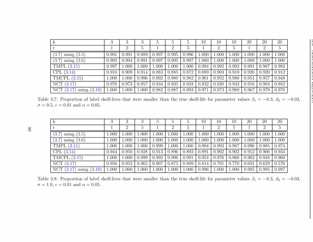
3.3
.SIM
ULA
TIO
NR
ESU
LT
S
k 3 3 3 5 5 5 10 10 10 20 20 20r 1 2 5 1 2 5 1 2 5 1 2 5
(3.7) using (3.5) 0.991 0.991 0.989 0.997 0.995 0.996 1.000 1.000 1.000 1.000 1.000 1.000(3.7) using (3.6) 0.993 0.994 0.991 0.997 0.995 0.997 1.000 1.000 1.000 1.000 1.000 1.000TMPL (3.11) 0.997 1.000 1.000 1.000 1.000 1.000 0.994 0.992 0.993 0.991 0.987 0.982CPL (3.14) 0.910 0.909 0.914 0.883 0.885 0.872 0.889 0.903 0.919 0.926 0.920 0.912TMCPL (3.15) 1.000 1.000 0.996 0.992 0.980 0.982 0.961 0.952 0.980 0.951 0.957 0.948NCT (3.17) 0.970 0.973 0.957 0.934 0.935 0.933 0.932 0.920 0.943 0.916 0.904 0.882NCT (3.17) using (3.19) 1.000 1.000 1.000 0.982 0.987 0.993 0.971 0.973 0.989 0.967 0.979 0.978
Table 3.7: Proportion of label shelf-lives that were smaller than the true shelf-life for parameter values β1 = −0.3, d2 = −0.03,σ = 0.5, ε = 0.01 and α = 0.05.
k 3 3 3 5 5 5 10 10 10 20 20 20r 1 2 5 1 2 5 1 2 5 1 2 5
(3.7) using (3.5) 1.000 1.000 1.000 1.000 1.000 1.000 1.000 1.000 1.000 1.000 1.000 1.000(3.7) using (3.6) 1.000 1.000 1.000 1.000 1.000 1.000 1.000 1.000 1.000 1.000 1.000 1.000TMPL (3.11) 1.000 1.000 1.000 0.999 1.000 1.000 0.994 0.993 0.987 0.996 0.985 0.974CPL (3.14) 0.944 0.950 0.928 0.913 0.896 0.893 0.891 0.902 0.902 0.912 0.906 0.934TMCPL (3.15) 1.000 1.000 0.999 0.992 0.996 0.991 0.954 0.976 0.966 0.962 0.948 0.960NCT (3.17) 0.956 0.953 0.965 0.907 0.875 0.889 0.814 0.791 0.770 0.691 0.629 0.576NCT (3.17) using (3.19) 1.000 1.000 1.000 1.000 1.000 1.000 0.996 1.000 1.000 0.995 0.995 0.997
Table 3.8: Proportion of label shelf-lives that were smaller than the true shelf-life for parameter values β1 = −0.3, d2 = −0.03,σ = 1.0, ε = 0.01 and α = 0.05.
99
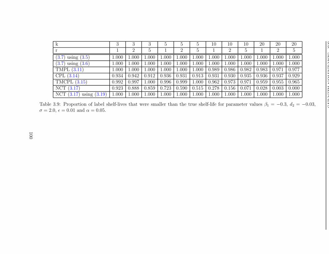
3.3
.SIM
ULA
TIO
NR
ESU
LT
S
k 3 3 3 5 5 5 10 10 10 20 20 20r 1 2 5 1 2 5 1 2 5 1 2 5
(3.7) using (3.5) 1.000 1.000 1.000 1.000 1.000 1.000 1.000 1.000 1.000 1.000 1.000 1.000(3.7) using (3.6) 1.000 1.000 1.000 1.000 1.000 1.000 1.000 1.000 1.000 1.000 1.000 1.000TMPL (3.11) 1.000 1.000 1.000 1.000 1.000 1.000 0.989 0.986 0.982 0.983 0.971 0.977CPL (3.14) 0.934 0.942 0.912 0.936 0.931 0.913 0.931 0.930 0.935 0.936 0.937 0.929TMCPL (3.15) 0.992 0.997 1.000 0.996 0.999 1.000 0.962 0.973 0.971 0.959 0.955 0.965NCT (3.17) 0.923 0.888 0.859 0.723 0.590 0.515 0.278 0.156 0.071 0.028 0.003 0.000NCT (3.17) using (3.19) 1.000 1.000 1.000 1.000 1.000 1.000 1.000 1.000 1.000 1.000 1.000 1.000
Table 3.9: Proportion of label shelf-lives that were smaller than the true shelf-life for parameter values β1 = −0.3, d2 = −0.03,σ = 2.0, ε = 0.01 and α = 0.05.
100
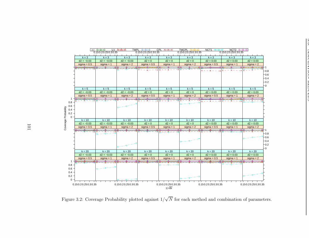
3.3
.SIM
ULA
TIO
NR
ESU
LT
S
1 8r
Cov
erag
e P
roba
bilit
ysigma = 0.5d2 = −0.03
k = 3
sigma = 1d2 = −0.03
k = 3
0.150.20.25 0.30.35
sigma = 2d2 = −0.03
k = 3
sigma = 0.5d2 = 0k = 3
0.15 0.20.25 0.30.35
sigma = 1d2 = 0k = 3
sigma = 2d2 = 0k = 3
0.15 0.20.25 0.30.35
sigma = 0.5d2 = 0.03
k = 3
sigma = 1d2 = 0.03
k = 3
0.15 0.20.250.3 0.35
00.20.40.60.81
sigma = 2d2 = 0.03
k = 3
00.20.40.60.8
1sigma = 0.5d2 = −0.03
k = 5
sigma = 1d2 = −0.03
k = 5
sigma = 2d2 = −0.03
k = 5
sigma = 0.5d2 = 0k = 5
sigma = 1d2 = 0k = 5
sigma = 2d2 = 0k = 5
sigma = 0.5d2 = 0.03
k = 5
sigma = 1d2 = 0.03
k = 5
sigma = 2d2 = 0.03
k = 5
sigma = 0.5d2 = −0.03
k = 10
sigma = 1d2 = −0.03
k = 10
sigma = 2d2 = −0.03
k = 10
sigma = 0.5d2 = 0k = 10
sigma = 1d2 = 0k = 10
sigma = 2d2 = 0k = 10
sigma = 0.5d2 = 0.03
k = 10
sigma = 1d2 = 0.03
k = 10
00.20.40.60.81
sigma = 2d2 = 0.03
k = 10
00.20.40.60.8
1
0.15 0.20.250.3 0.35
sigma = 0.5d2 = −0.03
k = 20
sigma = 1d2 = −0.03
k = 20
0.150.2 0.250.3 0.35
sigma = 2d2 = −0.03
k = 20
sigma = 0.5d2 = 0k = 20
0.150.2 0.250.3 0.35
sigma = 1d2 = 0k = 20
sigma = 2d2 = 0k = 20
0.150.2 0.250.30.35
sigma = 0.5d2 = 0.03
k = 20
sigma = 1d2 = 0.03
k = 20
0.150.20.25 0.30.35
sigma = 2d2 = 0.03
k = 20
z.t U.t TMPL CPL TMCPL NCT1 NCT2
Figure 3.2: Coverage Probability plotted against 1/√N for each method and combination of parameters.
101

3.3
.SIM
ULA
TIO
NR
ESU
LT
S
k 3 3 3 5 5 5 10 10 10 20 20 20r 1 2 5 1 2 5 1 2 5 1 2 5
(3.7) using (3.5) −17.3 −16.3 −15.3 −13.9 −13.7 −13.3 −12.6 −12.6 −12.6 −12.0 −11.9 −11.9(3.7) using (3.6) −17.8 −16.9 −15.8 −14.4 −14.2 −13.9 −12.9 −12.9 −12.9 −12.2 −12.1 −12.0TMPL (3.11) −20.8 −20.7 −20.9 −20.8 −20.9 −20.9 −17.9 −17.9 −15.2 −14.0 −13.7 −13.5CPL (3.14) −7.7 −7.2 −7.5 −4.9 −5.1 −5.1 −3.6 −3.7 −3.6 −2.6 −2.6 −2.6TMCPL (3.15) −13.0 −12.5 −12.3 −7.8 −7.9 −7.7 −4.7 −4.7 −4.5 −3.1 −3.1 −2.9NCT (3.17) −15.4 −15.0 −14.8 −8.6 −9.0 −8.7 −4.7 −4.7 −4.6 −2.9 −2.8 −2.7NCT (3.17) using (3.19) −17.6 −17.2 −17.2 −9.8 −10.3 −10.1 −5.4 −5.5 −5.5 −3.4 −3.4 −3.4
Table 3.10: Bias of label shelf-lives for parameter values β1 = −0.3, d2 = 0.00, σ = 0.5, ε = 0.01 and α = 0.05.
k 3 3 3 5 5 5 10 10 10 20 20 20r 1 2 5 1 2 5 1 2 5 1 2 5
(3.7) using (3.5) −18.5 −17.5 −16.8 −17.0 −15.9 −15.4 −15.5 −15.0 −14.6 −14.7 −14.3 −14.3(3.7) using (3.6) −18.6 −17.7 −17.0 −17.2 −16.1 −15.7 −15.7 −15.1 −14.7 −14.8 −14.4 −14.4TMPL (3.11) −18.6 −19.0 −19.4 −19.0 −19.3 −19.4 −15.3 −14.5 −13.2 −13.2 −11.3 −10.4CPL (3.14) −7.7 −6.8 −6.4 −5.3 −4.8 −4.9 −3.5 −3.4 −3.3 −2.5 −2.4 −2.5TMCPL (3.15) −13.3 −13.2 −12.4 −7.8 −7.6 −7.6 −4.6 −4.5 −4.3 −3.0 −2.9 −3.0NCT (3.17) −14.7 −14.4 −13.7 −8.3 −7.6 −7.7 −3.7 −3.5 −3.3 −1.8 −1.6 −1.6NCT (3.17) using (3.19) −19.1 −19.3 −19.5 −12.9 −12.6 −13.0 −6.5 −6.5 −6.4 −4.0 −3.9 −4.1
Table 3.11: Bias of label shelf-lives for parameter values β1 = −0.3, d2 = 0.00, σ = 1.0, ε = 0.01 and α = 0.05.
102

3.3
.SIM
ULA
TIO
NR
ESU
LT
S
k 3 3 3 5 5 5 10 10 10 20 20 20r 1 2 5 1 2 5 1 2 5 1 2 5
(3.7) using (3.5) −14.8 −14.9 −14.9 −14.9 −14.9 −14.9 −14.9 −14.9 −14.9 −14.9 −14.9 −14.9(3.7) using (3.6) −14.9 −14.9 −14.9 −14.9 −14.9 −14.9 −14.9 −14.9 −14.9 −14.9 −14.9 −14.9TMPL (3.11) −14.4 −14.7 −14.7 −14.7 −14.5 −14.1 −8.3 −7.5 −6.2 −4.7 −4.7 −3.2CPL (3.14) −8.1 −7.0 −5.6 −5.6 −4.9 −4.1 −3.8 −3.1 −2.9 −2.5 −2.2 −2.1TMCPL (3.15) −10.5 −10.9 −9.6 −7.0 −6.6 −6.1 −4.3 −3.8 −3.7 −2.8 −2.5 −2.4NCT (3.17) −12.1 −10.8 −9.7 −5.9 −4.4 −3.2 −0.5 0.7 1.0 1.9 2.6 2.9NCT (3.17) using (3.19) −14.9 −14.9 −14.9 −14.6 −14.8 −14.9 −10.6 −10.4 −10.5 −6.1 −6.0 −6.1
Table 3.12: Bias of label shelf-lives for parameter values β1 = −0.3, d2 = 0.00, σ = 2.0, ε = 0.01 and α = 0.05.
k 3 3 3 5 5 5 10 10 10 20 20 20r 1 2 5 1 2 5 1 2 5 1 2 5
(3.7) using (3.5) −16.2 −15.4 −14.3 −14.2 −13.4 −12.9 −12.8 −12.7 −12.4 −12.2 −12.1 −12.2(3.7) using (3.6) −16.5 −15.8 −14.8 −14.7 −13.9 −13.3 −13.1 −13.0 −12.7 −12.4 −12.2 −12.3TMPL (3.11) −18.7 −18.8 −18.9 −18.9 −18.9 −18.9 −18.5 −18.5 −14.7 −5.3 −4.6 −3.8CPL (3.14) −6.3 −6.5 −6.5 −5.4 −5.3 −5.0 −4.0 −4.1 −3.7 −2.9 −2.8 −2.9TMCPL (3.15) −12.1 −11.7 −11.4 −8.0 −7.5 −7.2 −4.9 −5.0 −4.6 −3.4 −3.2 −3.3NCT (3.17) −13.8 −13.9 −13.6 −9.4 −9.2 −8.9 −5.2 −5.3 −4.9 −3.3 −3.1 −3.2NCT (3.17) using (3.19) −15.7 −15.8 −15.8 −10.3 −10.3 −10.0 −5.8 −5.9 −5.6 −3.8 −3.6 −3.7
Table 3.13: Bias of label shelf-lives for parameter values β1 = −0.3, d2 = 0.03, σ = 0.5, ε = 0.01 and α = 0.05.
103

3.3
.SIM
ULA
TIO
NR
ESU
LT
S
k 3 3 3 5 5 5 10 10 10 20 20 20r 1 2 5 1 2 5 1 2 5 1 2 5
(3.7) using (3.5) −16.8 −16.5 −15.8 −16.1 −15.5 −14.6 −15.2 −14.3 −14.2 −14.2 −13.8 −13.8(3.7) using (3.6) −16.9 −16.6 −15.9 −16.2 −15.7 −14.8 −15.3 −14.4 −14.3 −14.3 −13.8 −13.8TMPL (3.11) −16.7 −17.5 −17.6 −17.3 −17.6 −17.7 −15.5 −15.1 −15.3 −9.7 −6.3 −4.8CPL (3.14) −6.4 −6.5 −6.3 −5.2 −5.2 −5.2 −3.9 −3.5 −3.9 −2.8 −2.6 −2.7TMCPL (3.15) −12.1 −12.3 −12.0 −7.4 −7.5 −7.6 −4.8 −4.5 −4.8 −3.2 −3.1 −3.2NCT (3.17) −13.3 −13.3 −13.0 −8.5 −8.3 −8.2 −4.4 −3.9 −4.2 −2.3 −2.1 −2.1NCT (3.17) using (3.19) −17.2 −17.5 −17.7 −12.1 −12.2 −12.2 −6.7 −6.4 −6.8 −4.2 −4.1 −4.2
Table 3.14: Bias of label shelf-lives for parameter values β1 = −0.3, d2 = 0.03, σ = 1.0, ε = 0.01 and α = 0.05.
k 3 3 3 5 5 5 10 10 10 20 20 20r 1 2 5 1 2 5 1 2 5 1 2 5
(3.7) using (3.5) −13.7 −13.7 −13.7 −13.7 −13.7 −13.7 −13.7 −13.7 −13.7 −13.7 −13.7 −13.7(3.7) using (3.6) −13.7 −13.7 −13.7 −13.7 −13.7 −13.7 −13.7 −13.7 −13.7 −13.7 −13.7 −13.7TMPL (3.11) −13.2 −13.5 −13.6 −13.5 −13.4 −13.2 −8.4 −7.4 −6.6 −4.7 −4.5 −3.5CPL (3.14) −7.0 −6.1 −5.0 −5.5 −4.9 −4.5 −3.9 −3.4 −3.1 −2.8 −2.5 −2.3TMCPL (3.15) −9.8 −9.9 −8.7 −6.6 −6.4 −6.1 −4.3 −4.0 −3.8 −3.0 −2.7 −2.6NCT (3.17) −10.9 −9.8 −8.9 −6.3 −5.1 −4.5 −1.5 −0.7 −0.1 0.8 1.4 1.8NCT (3.17) using (3.19) −13.7 −13.7 −13.7 −13.5 −13.7 −13.7 −9.8 −9.7 −9.8 −6.0 −5.9 −5.8
Table 3.15: Bias of label shelf-lives for parameter values β1 = −0.3, d2 = 0.03, σ = 2.0, ε = 0.01 and α = 0.05.
104
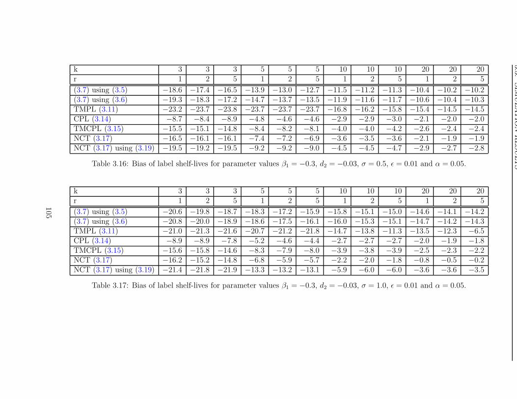
3.3
.SIM
ULA
TIO
NR
ESU
LT
S
k 3 3 3 5 5 5 10 10 10 20 20 20r 1 2 5 1 2 5 1 2 5 1 2 5
(3.7) using (3.5) −18.6 −17.4 −16.5 −13.9 −13.0 −12.7 −11.5 −11.2 −11.3 −10.4 −10.2 −10.2(3.7) using (3.6) −19.3 −18.3 −17.2 −14.7 −13.7 −13.5 −11.9 −11.6 −11.7 −10.6 −10.4 −10.3TMPL (3.11) −23.2 −23.7 −23.8 −23.7 −23.7 −23.7 −16.8 −16.2 −15.8 −15.4 −14.5 −14.5CPL (3.14) −8.7 −8.4 −8.9 −4.8 −4.6 −4.6 −2.9 −2.9 −3.0 −2.1 −2.0 −2.0TMCPL (3.15) −15.5 −15.1 −14.8 −8.4 −8.2 −8.1 −4.0 −4.0 −4.2 −2.6 −2.4 −2.4NCT (3.17) −16.5 −16.1 −16.1 −7.4 −7.2 −6.9 −3.6 −3.5 −3.6 −2.1 −1.9 −1.9NCT (3.17) using (3.19) −19.5 −19.2 −19.5 −9.2 −9.2 −9.0 −4.5 −4.5 −4.7 −2.9 −2.7 −2.8
Table 3.16: Bias of label shelf-lives for parameter values β1 = −0.3, d2 = −0.03, σ = 0.5, ε = 0.01 and α = 0.05.
k 3 3 3 5 5 5 10 10 10 20 20 20r 1 2 5 1 2 5 1 2 5 1 2 5
(3.7) using (3.5) −20.6 −19.8 −18.7 −18.3 −17.2 −15.9 −15.8 −15.1 −15.0 −14.6 −14.1 −14.2(3.7) using (3.6) −20.8 −20.0 −18.9 −18.6 −17.5 −16.1 −16.0 −15.3 −15.1 −14.7 −14.2 −14.3TMPL (3.11) −21.0 −21.3 −21.6 −20.7 −21.2 −21.8 −14.7 −13.8 −11.3 −13.5 −12.3 −6.5CPL (3.14) −8.9 −8.9 −7.8 −5.2 −4.6 −4.4 −2.7 −2.7 −2.7 −2.0 −1.9 −1.8TMCPL (3.15) −15.6 −15.8 −14.6 −8.3 −7.9 −8.0 −3.9 −3.8 −3.9 −2.5 −2.3 −2.2NCT (3.17) −16.2 −15.2 −14.8 −6.8 −5.9 −5.7 −2.2 −2.0 −1.8 −0.8 −0.5 −0.2NCT (3.17) using (3.19) −21.4 −21.8 −21.9 −13.3 −13.2 −13.1 −5.9 −6.0 −6.0 −3.6 −3.6 −3.5
Table 3.17: Bias of label shelf-lives for parameter values β1 = −0.3, d2 = −0.03, σ = 1.0, ε = 0.01 and α = 0.05.
105
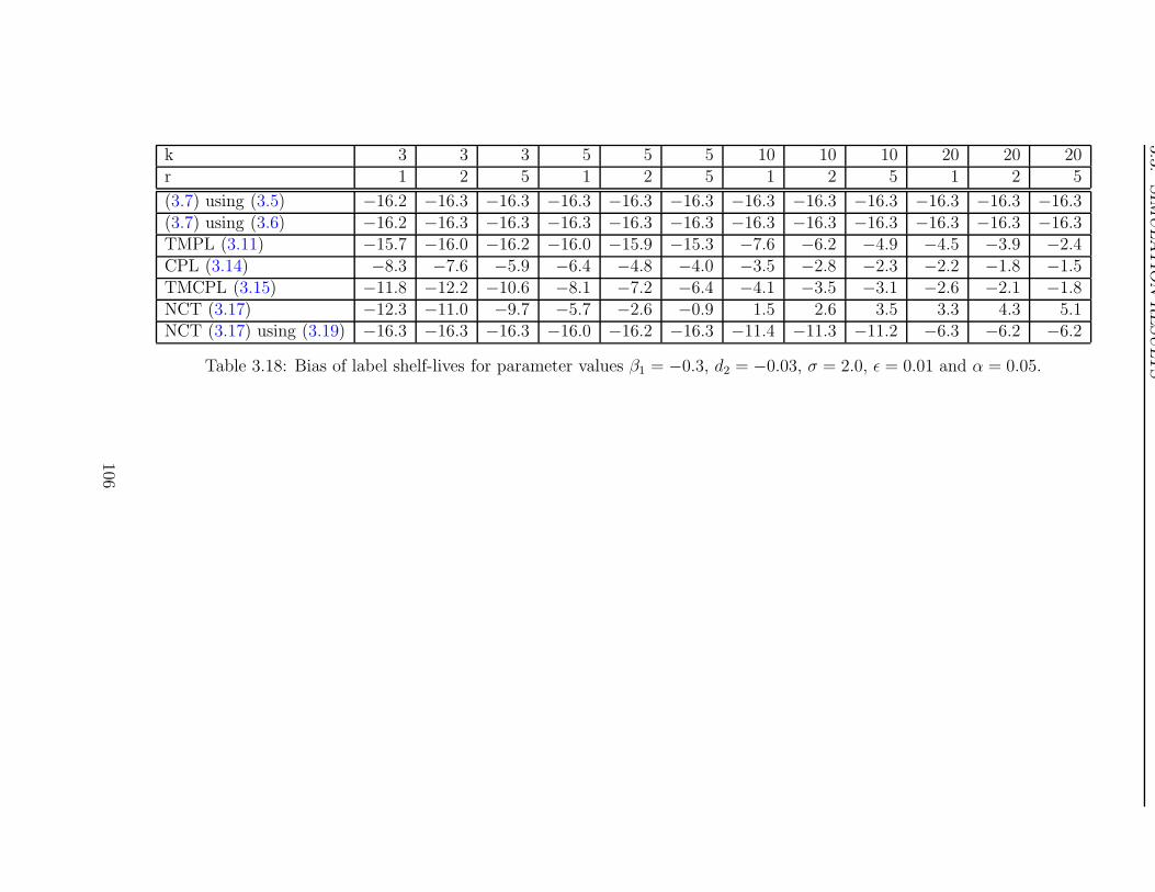
3.3
.SIM
ULA
TIO
NR
ESU
LT
S
k 3 3 3 5 5 5 10 10 10 20 20 20r 1 2 5 1 2 5 1 2 5 1 2 5
(3.7) using (3.5) −16.2 −16.3 −16.3 −16.3 −16.3 −16.3 −16.3 −16.3 −16.3 −16.3 −16.3 −16.3(3.7) using (3.6) −16.2 −16.3 −16.3 −16.3 −16.3 −16.3 −16.3 −16.3 −16.3 −16.3 −16.3 −16.3TMPL (3.11) −15.7 −16.0 −16.2 −16.0 −15.9 −15.3 −7.6 −6.2 −4.9 −4.5 −3.9 −2.4CPL (3.14) −8.3 −7.6 −5.9 −6.4 −4.8 −4.0 −3.5 −2.8 −2.3 −2.2 −1.8 −1.5TMCPL (3.15) −11.8 −12.2 −10.6 −8.1 −7.2 −6.4 −4.1 −3.5 −3.1 −2.6 −2.1 −1.8NCT (3.17) −12.3 −11.0 −9.7 −5.7 −2.6 −0.9 1.5 2.6 3.5 3.3 4.3 5.1NCT (3.17) using (3.19) −16.3 −16.3 −16.3 −16.0 −16.2 −16.3 −11.4 −11.3 −11.2 −6.3 −6.2 −6.2
Table 3.18: Bias of label shelf-lives for parameter values β1 = −0.3, d2 = −0.03, σ = 2.0, ε = 0.01 and α = 0.05.
106
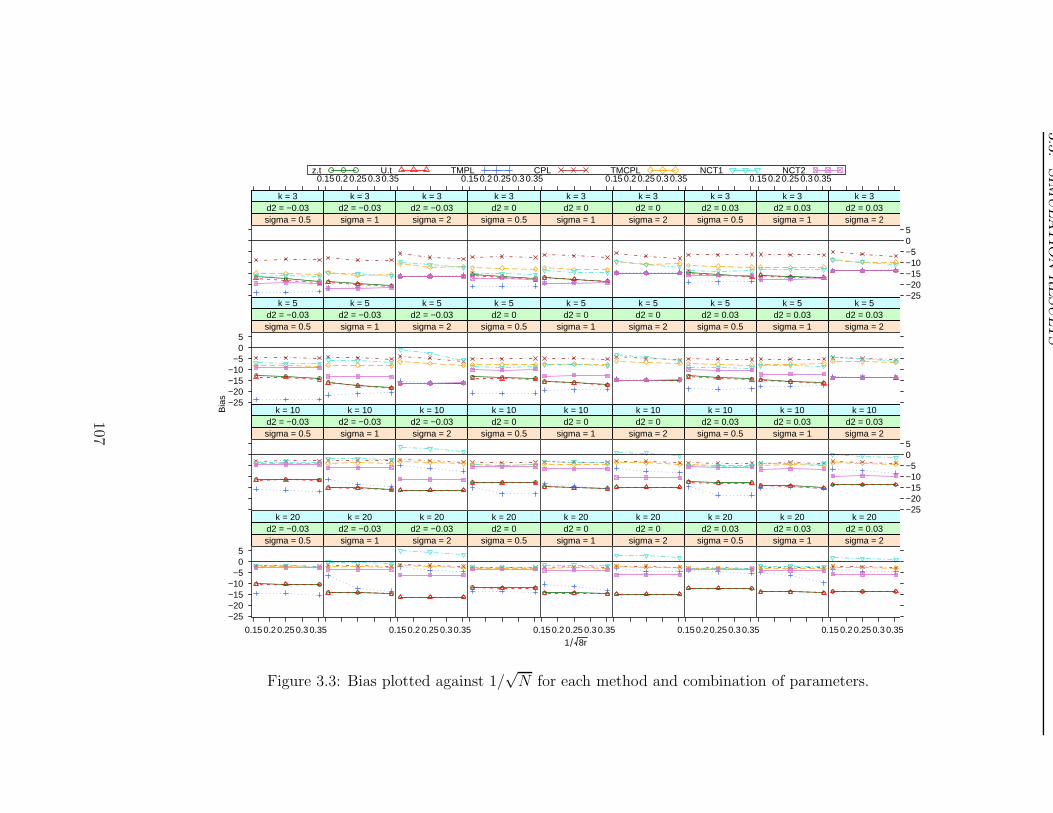
3.3
.SIM
ULA
TIO
NR
ESU
LT
S
1 8r
Bia
ssigma = 0.5d2 = −0.03
k = 3
sigma = 1d2 = −0.03
k = 3
0.15 0.2 0.25 0.3 0.35
sigma = 2d2 = −0.03
k = 3
sigma = 0.5d2 = 0k = 3
0.15 0.2 0.25 0.3 0.35
sigma = 1d2 = 0k = 3
sigma = 2d2 = 0k = 3
0.15 0.2 0.25 0.3 0.35
sigma = 0.5d2 = 0.03
k = 3
sigma = 1d2 = 0.03
k = 3
0.15 0.2 0.25 0.3 0.35
−25−20−15−10−505
sigma = 2d2 = 0.03
k = 3
−25−20−15−10
−505
sigma = 0.5d2 = −0.03
k = 5
sigma = 1d2 = −0.03
k = 5
sigma = 2d2 = −0.03
k = 5
sigma = 0.5d2 = 0k = 5
sigma = 1d2 = 0k = 5
sigma = 2d2 = 0k = 5
sigma = 0.5d2 = 0.03
k = 5
sigma = 1d2 = 0.03
k = 5
sigma = 2d2 = 0.03
k = 5
sigma = 0.5d2 = −0.03
k = 10
sigma = 1d2 = −0.03
k = 10
sigma = 2d2 = −0.03
k = 10
sigma = 0.5d2 = 0k = 10
sigma = 1d2 = 0k = 10
sigma = 2d2 = 0k = 10
sigma = 0.5d2 = 0.03
k = 10
sigma = 1d2 = 0.03
k = 10
−25−20−15−10−505
sigma = 2d2 = 0.03
k = 10
−25−20−15−10
−505
0.15 0.2 0.25 0.3 0.35
sigma = 0.5d2 = −0.03
k = 20
sigma = 1d2 = −0.03
k = 20
0.15 0.2 0.25 0.3 0.35
sigma = 2d2 = −0.03
k = 20
sigma = 0.5d2 = 0k = 20
0.15 0.2 0.25 0.3 0.35
sigma = 1d2 = 0k = 20
sigma = 2d2 = 0k = 20
0.15 0.2 0.25 0.3 0.35
sigma = 0.5d2 = 0.03
k = 20
sigma = 1d2 = 0.03
k = 20
0.15 0.2 0.25 0.3 0.35
sigma = 2d2 = 0.03
k = 20
z.t U.t TMPL CPL TMCPL NCT1 NCT2
Figure 3.3: Bias plotted against 1/√N for each method and combination of parameters.
107
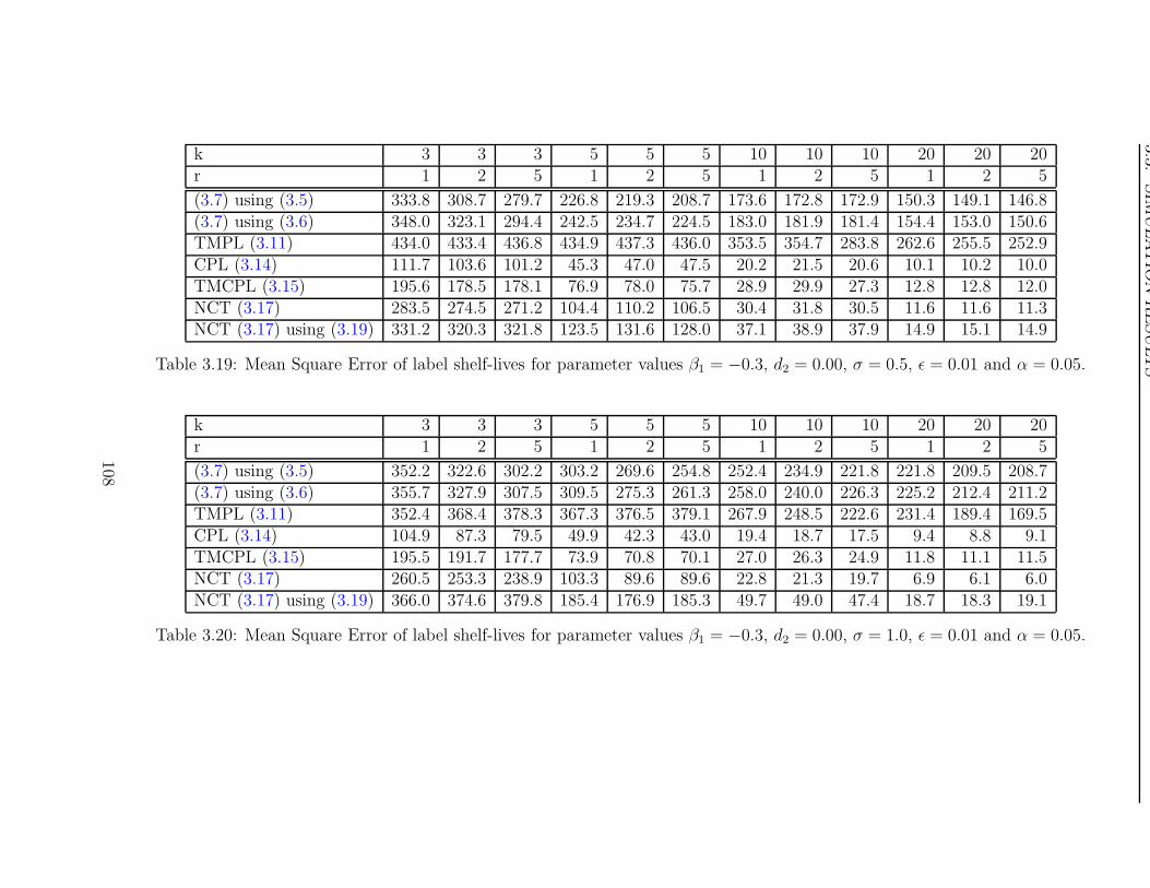
3.3
.SIM
ULA
TIO
NR
ESU
LT
S
k 3 3 3 5 5 5 10 10 10 20 20 20r 1 2 5 1 2 5 1 2 5 1 2 5
(3.7) using (3.5) 333.8 308.7 279.7 226.8 219.3 208.7 173.6 172.8 172.9 150.3 149.1 146.8(3.7) using (3.6) 348.0 323.1 294.4 242.5 234.7 224.5 183.0 181.9 181.4 154.4 153.0 150.6TMPL (3.11) 434.0 433.4 436.8 434.9 437.3 436.0 353.5 354.7 283.8 262.6 255.5 252.9CPL (3.14) 111.7 103.6 101.2 45.3 47.0 47.5 20.2 21.5 20.6 10.1 10.2 10.0TMCPL (3.15) 195.6 178.5 178.1 76.9 78.0 75.7 28.9 29.9 27.3 12.8 12.8 12.0NCT (3.17) 283.5 274.5 271.2 104.4 110.2 106.5 30.4 31.8 30.5 11.6 11.6 11.3NCT (3.17) using (3.19) 331.2 320.3 321.8 123.5 131.6 128.0 37.1 38.9 37.9 14.9 15.1 14.9
Table 3.19: Mean Square Error of label shelf-lives for parameter values β1 = −0.3, d2 = 0.00, σ = 0.5, ε = 0.01 and α = 0.05.
k 3 3 3 5 5 5 10 10 10 20 20 20r 1 2 5 1 2 5 1 2 5 1 2 5
(3.7) using (3.5) 352.2 322.6 302.2 303.2 269.6 254.8 252.4 234.9 221.8 221.8 209.5 208.7(3.7) using (3.6) 355.7 327.9 307.5 309.5 275.3 261.3 258.0 240.0 226.3 225.2 212.4 211.2TMPL (3.11) 352.4 368.4 378.3 367.3 376.5 379.1 267.9 248.5 222.6 231.4 189.4 169.5CPL (3.14) 104.9 87.3 79.5 49.9 42.3 43.0 19.4 18.7 17.5 9.4 8.8 9.1TMCPL (3.15) 195.5 191.7 177.7 73.9 70.8 70.1 27.0 26.3 24.9 11.8 11.1 11.5NCT (3.17) 260.5 253.3 238.9 103.3 89.6 89.6 22.8 21.3 19.7 6.9 6.1 6.0NCT (3.17) using (3.19) 366.0 374.6 379.8 185.4 176.9 185.3 49.7 49.0 47.4 18.7 18.3 19.1
Table 3.20: Mean Square Error of label shelf-lives for parameter values β1 = −0.3, d2 = 0.00, σ = 1.0, ε = 0.01 and α = 0.05.
108
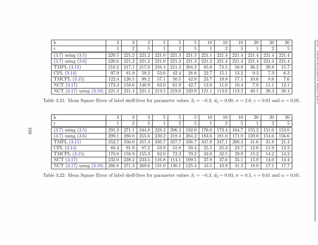
3.3
.SIM
ULA
TIO
NR
ESU
LT
S
k 3 3 3 5 5 5 10 10 10 20 20 20r 1 2 5 1 2 5 1 2 5 1 2 5
(3.7) using (3.5) 220.5 221.2 221.2 221.0 221.3 221.3 221.1 221.4 221.4 221.4 221.4 221.4(3.7) using (3.6) 220.6 221.2 221.2 221.0 221.3 221.3 221.2 221.4 221.4 221.4 221.4 221.4TMPL (3.11) 210.2 217.1 217.6 216.4 211.3 204.2 85.6 74.5 50.9 36.2 39.8 15.7CPL (3.14) 97.9 81.9 59.2 53.6 42.4 28.8 22.7 15.1 13.2 9.3 7.3 6.3TMCPL (3.15) 122.4 126.5 98.2 57.1 50.5 42.9 23.7 18.8 17.1 10.6 8.6 7.6NCT (3.17) 173.3 158.6 140.9 83.0 61.9 42.7 13.8 11.0 10.4 7.8 11.1 12.1NCT (3.17) using (3.19) 221.3 221.4 221.4 213.5 219.0 220.9 121.1 113.6 113.2 40.1 38.3 38.4
Table 3.21: Mean Square Error of label shelf-lives for parameter values β1 = −0.3, d2 = 0.00, σ = 2.0, ε = 0.01 and α = 0.05.
k 3 3 3 5 5 5 10 10 10 20 20 20r 1 2 5 1 2 5 1 2 5 1 2 5
(3.7) using (3.5) 291.3 271.1 244.8 228.2 206.3 192.0 176.0 173.4 164.7 155.2 151.0 153.0(3.7) using (3.6) 299.1 280.8 255.6 239.2 218.4 204.2 183.6 181.0 171.9 159.0 154.6 156.6TMPL (3.11) 352.7 356.0 357.4 356.7 357.7 356.7 347.8 347.1 260.4 41.6 31.8 21.4CPL (3.14) 88.4 91.9 87.2 53.9 51.8 50.4 25.5 25.3 23.7 12.6 11.9 12.3TMCPL (3.15) 170.6 158.9 155.3 82.0 72.3 70.2 33.0 32.5 29.9 15.2 14.2 14.2NCT (3.17) 232.0 238.2 233.5 116.8 114.1 109.5 37.8 37.6 35.1 15.0 14.0 14.4NCT (3.17) using (3.19) 266.8 271.3 269.6 131.0 130.1 125.4 43.5 43.9 41.3 18.0 17.1 17.7
Table 3.22: Mean Square Error of label shelf-lives for parameter values β1 = −0.3, d2 = 0.03, σ = 0.5, ε = 0.01 and α = 0.05.
109
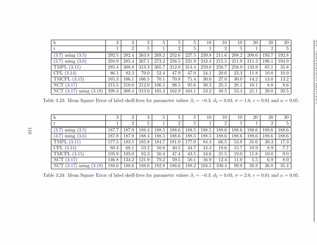
3.3
.SIM
ULA
TIO
NR
ESU
LT
S
k 3 3 3 5 5 5 10 10 10 20 20 20r 1 2 5 1 2 5 1 2 5 1 2 5
(3.7) using (3.5) 292.5 282.4 263.8 269.2 252.6 227.5 239.8 211.6 208.2 208.6 193.7 192.8(3.7) using (3.6) 294.9 285.4 267.1 273.2 256.5 231.9 243.4 215.5 211.9 211.3 196.1 194.9TMPL (3.11) 285.4 308.9 313.3 305.7 312.0 314.4 259.0 250.7 258.9 133.9 65.1 35.8CPL (3.14) 86.1 82.3 79.0 52.4 47.9 47.0 24.1 20.6 23.3 11.8 10.8 10.9TMCPL (3.15) 165.3 166.1 166.5 70.1 70.8 71.4 30.6 27.0 30.0 14.2 13.0 13.2NCT (3.17) 215.5 218.0 212.0 106.5 96.5 95.6 30.3 25.5 28.1 10.1 8.8 8.6NCT (3.17) using (3.19) 298.3 308.4 313.6 165.3 162.9 164.1 53.2 48.5 53.4 21.1 20.0 20.5
Table 3.23: Mean Square Error of label shelf-lives for parameter values β1 = −0.3, d2 = 0.03, σ = 1.0, ε = 0.01 and α = 0.05.
k 3 3 3 5 5 5 10 10 10 20 20 20r 1 2 5 1 2 5 1 2 5 1 2 5
(3.7) using (3.5) 187.7 187.9 188.4 188.5 188.6 188.5 188.5 188.6 188.6 188.6 188.6 188.6(3.7) using (3.6) 187.8 187.9 188.4 188.5 188.6 188.5 188.5 188.6 188.6 188.6 188.6 188.6TMPL (3.11) 177.5 183.5 185.8 184.7 181.0 177.0 84.4 66.5 53.8 31.6 30.3 17.3CPL (3.14) 80.3 68.1 53.2 50.8 40.5 34.7 24.3 18.6 15.7 10.9 8.9 7.7TMCPL (3.15) 105.9 105.0 82.3 50.4 47.4 43.5 24.6 21.5 19.0 11.8 10.0 9.0NCT (3.17) 146.8 134.2 121.9 79.2 59.5 50.1 16.9 12.4 11.0 5.5 6.9 8.0NCT (3.17) using (3.19) 188.6 188.6 188.6 182.8 186.6 188.2 104.5 100.4 99.8 38.8 36.8 35.4
Table 3.24: Mean Square Error of label shelf-lives for parameter values β1 = −0.3, d2 = 0.03, σ = 2.0, ε = 0.01 and α = 0.05.
110

3.3
.SIM
ULA
TIO
NR
ESU
LT
S
k 3 3 3 5 5 5 10 10 10 20 20 20r 1 2 5 1 2 5 1 2 5 1 2 5
(3.7) using (3.5) 400.2 361.0 332.2 240.4 212.4 202.2 150.4 141.7 142.9 114.6 110.5 108.9(3.7) using (3.6) 422.6 387.9 356.7 265.1 233.0 226.3 162.1 152.6 154.0 117.8 113.5 111.7TMPL (3.11) 548.6 563.1 564.7 563.1 563.7 561.1 359.5 345.7 336.2 338.1 318.5 322.8CPL (3.14) 143.8 131.8 142.3 47.8 44.0 46.7 13.6 13.8 14.9 6.6 5.7 5.8TMCPL (3.15) 273.1 258.3 255.3 95.5 89.0 92.9 21.8 22.2 23.4 9.0 7.8 7.5NCT (3.17) 337.4 323.3 328.8 84.0 78.5 74.8 18.7 17.8 18.5 6.9 5.8 5.8NCT (3.17) using (3.19) 411.5 400.1 410.7 111.6 108.1 105.1 25.9 25.5 26.9 10.4 9.4 9.5
Table 3.25: Mean Square Error of label shelf-lives for parameter values β1 = −0.3, d2 = −0.03, σ = 0.5, ε = 0.01 and α = 0.05.
k 3 3 3 5 5 5 10 10 10 20 20 20r 1 2 5 1 2 5 1 2 5 1 2 5
(3.7) using (3.5) 436.9 409.7 374.2 357.3 320.9 276.9 270.1 243.2 238.4 223.4 206.0 208.4(3.7) using (3.6) 443.6 416.4 380.7 367.1 330.9 284.8 277.3 249.8 244.1 227.6 209.2 211.1TMPL (3.11) 450.2 463.9 472.5 444.9 460.0 477.3 279.1 259.5 198.1 261.0 242.4 105.9CPL (3.14) 136.2 135.1 108.6 55.9 43.4 38.3 13.2 12.4 13.7 5.9 5.5 4.8TMCPL (3.15) 269.7 273.1 244.9 89.8 82.5 83.1 20.6 19.5 21.8 8.1 7.4 7.0NCT (3.17) 321.6 296.7 278.7 82.8 67.0 60.5 11.3 9.8 8.9 3.1 2.9 2.4NCT (3.17) using (3.19) 462.2 475.6 479.5 202.7 195.6 190.5 39.9 39.4 39.4 14.6 14.4 13.9
Table 3.26: Mean Square Error of label shelf-lives for parameter values β1 = −0.3, d2 = −0.03, σ = 1.0, ε = 0.01 and α = 0.05.
111
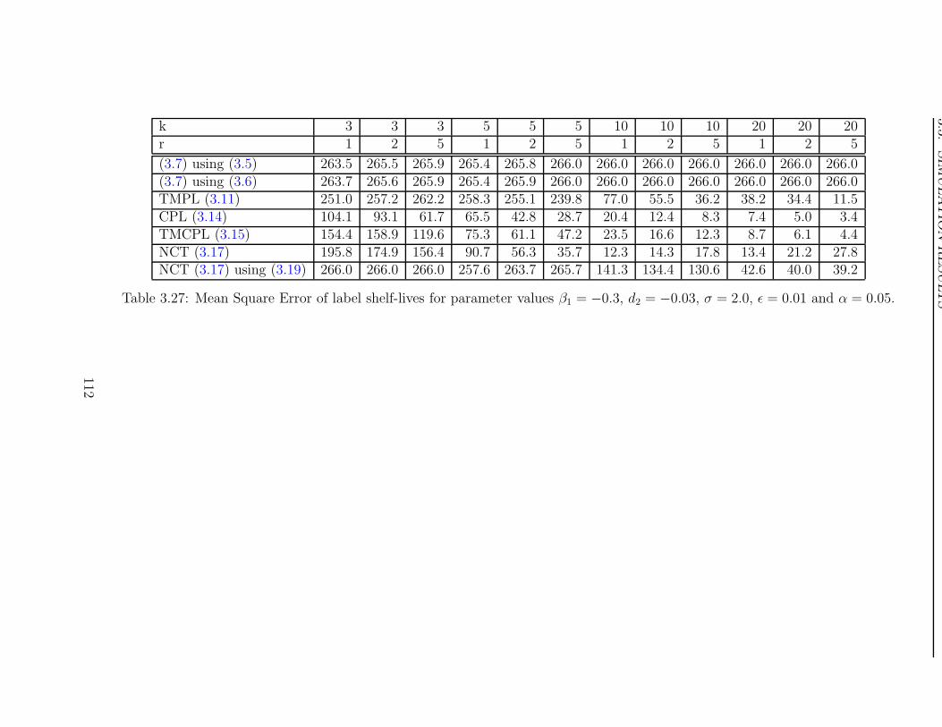
3.3
.SIM
ULA
TIO
NR
ESU
LT
S
k 3 3 3 5 5 5 10 10 10 20 20 20r 1 2 5 1 2 5 1 2 5 1 2 5
(3.7) using (3.5) 263.5 265.5 265.9 265.4 265.8 266.0 266.0 266.0 266.0 266.0 266.0 266.0(3.7) using (3.6) 263.7 265.6 265.9 265.4 265.9 266.0 266.0 266.0 266.0 266.0 266.0 266.0TMPL (3.11) 251.0 257.2 262.2 258.3 255.1 239.8 77.0 55.5 36.2 38.2 34.4 11.5CPL (3.14) 104.1 93.1 61.7 65.5 42.8 28.7 20.4 12.4 8.3 7.4 5.0 3.4TMCPL (3.15) 154.4 158.9 119.6 75.3 61.1 47.2 23.5 16.6 12.3 8.7 6.1 4.4NCT (3.17) 195.8 174.9 156.4 90.7 56.3 35.7 12.3 14.3 17.8 13.4 21.2 27.8NCT (3.17) using (3.19) 266.0 266.0 266.0 257.6 263.7 265.7 141.3 134.4 130.6 42.6 40.0 39.2
Table 3.27: Mean Square Error of label shelf-lives for parameter values β1 = −0.3, d2 = −0.03, σ = 2.0, ε = 0.01 and α = 0.05.
112
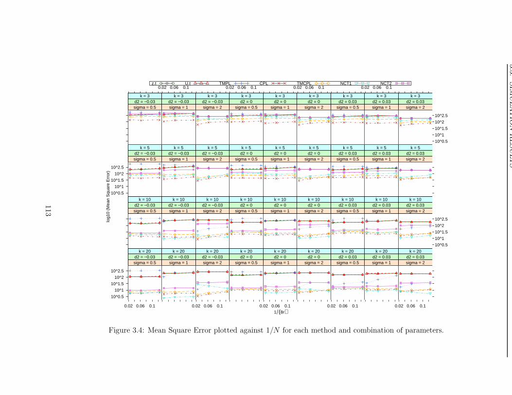
3.3
.SIM
ULA
TIO
NR
ESU
LT
S
1 (8r)
log1
0 (M
ean
Squ
are
Err
or)
sigma = 0.5d2 = −0.03
k = 3
sigma = 1d2 = −0.03
k = 3
0.02 0.06 0.1
sigma = 2d2 = −0.03
k = 3
sigma = 0.5d2 = 0k = 3
0.02 0.06 0.1
sigma = 1d2 = 0k = 3
sigma = 2d2 = 0k = 3
0.02 0.06 0.1
sigma = 0.5d2 = 0.03
k = 3
sigma = 1d2 = 0.03
k = 3
0.02 0.06 0.1
10^0.5
10^1
10^1.5
10^2
10^2.5
sigma = 2d2 = 0.03
k = 3
10^0.5
10^1
10^1.5
10^2
10^2.5
sigma = 0.5d2 = −0.03
k = 5
sigma = 1d2 = −0.03
k = 5
sigma = 2d2 = −0.03
k = 5
sigma = 0.5d2 = 0k = 5
sigma = 1d2 = 0k = 5
sigma = 2d2 = 0k = 5
sigma = 0.5d2 = 0.03
k = 5
sigma = 1d2 = 0.03
k = 5
sigma = 2d2 = 0.03
k = 5
sigma = 0.5d2 = −0.03
k = 10
sigma = 1d2 = −0.03
k = 10
sigma = 2d2 = −0.03
k = 10
sigma = 0.5d2 = 0k = 10
sigma = 1d2 = 0k = 10
sigma = 2d2 = 0k = 10
sigma = 0.5d2 = 0.03
k = 10
sigma = 1d2 = 0.03
k = 10
10^0.5
10^1
10^1.5
10^2
10^2.5
sigma = 2d2 = 0.03
k = 10
10^0.5
10^1
10^1.5
10^2
10^2.5
0.02 0.06 0.1
sigma = 0.5d2 = −0.03
k = 20
sigma = 1d2 = −0.03
k = 20
0.02 0.06 0.1
sigma = 2d2 = −0.03
k = 20
sigma = 0.5d2 = 0k = 20
0.02 0.06 0.1
sigma = 1d2 = 0k = 20
sigma = 2d2 = 0k = 20
0.02 0.06 0.1
sigma = 0.5d2 = 0.03
k = 20
sigma = 1d2 = 0.03
k = 20
0.02 0.06 0.1
sigma = 2d2 = 0.03
k = 20
z.t U.t TMPL CPL TMCPL NCT1 NCT2
Figure 3.4: Mean Square Error plotted against 1/N for each method and combination of parameters.
113
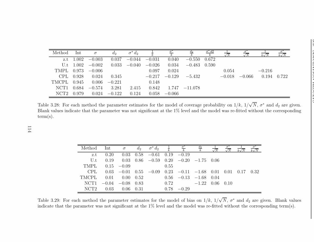
3.3
.SIM
ULA
TIO
NR
ESU
LT
S
Method Int σ d2 σ∗ d21k
σ∗
kd2
kσ∗ d2
k1√N
σ∗
√N
1k√
Nσ∗
k√
N
z.t 1.002 −0.003 0.037 −0.044 −0.031 0.040 −0.550 0.672U.t 1.002 −0.002 0.033 −0.040 −0.026 0.034 −0.483 0.590
TMPL 0.973 −0.006 0.097 0.024 0.054 −0.216CPL 0.928 0.024 0.345 −0.217 −0.129 −5.432 −0.018 −0.066 0.194 0.722
TMCPL 0.945 0.006 −0.221 0.148NCT1 0.684 −0.574 3.281 2.415 0.842 1.747 −11.078NCT2 0.979 0.024 −0.122 0.124 0.058 −0.066
Table 3.28: For each method the parameter estimates for the model of coverage probability on 1/k, 1/√N , σ∗ and d2 are given.
Blank values indicate that the parameter was not significant at the 1% level and the model was re-fitted without the correspondingterm(s).
Method Int σ d2 σ∗ d21k
σ∗
kd2
k1√N
σ∗
√N
1k√
Nσ∗
k√
N
z.t 0.20 0.03 0.58 −0.61 0.19 −0.19U.t 0.19 0.03 0.86 −0.59 0.20 −0.20 −1.75 0.06
TMPL 0.15 −0.09 0.55CPL 0.03 −0.01 0.55 −0.09 0.23 −0.11 −1.68 0.01 0.01 0.17 0.32
TMCPL 0.01 0.00 0.52 0.56 −0.13 −1.68 0.04NCT1 −0.04 −0.08 0.83 0.72 −1.22 0.06 0.10NCT2 0.03 0.06 0.31 0.78 −0.29
Table 3.29: For each method the parameter estimates for the model of bias on 1/k, 1/√N , σ∗ and d2 are given. Blank values
indicate that the parameter was not significant at the 1% level and the model was re-fitted without the corresponding term(s).
114
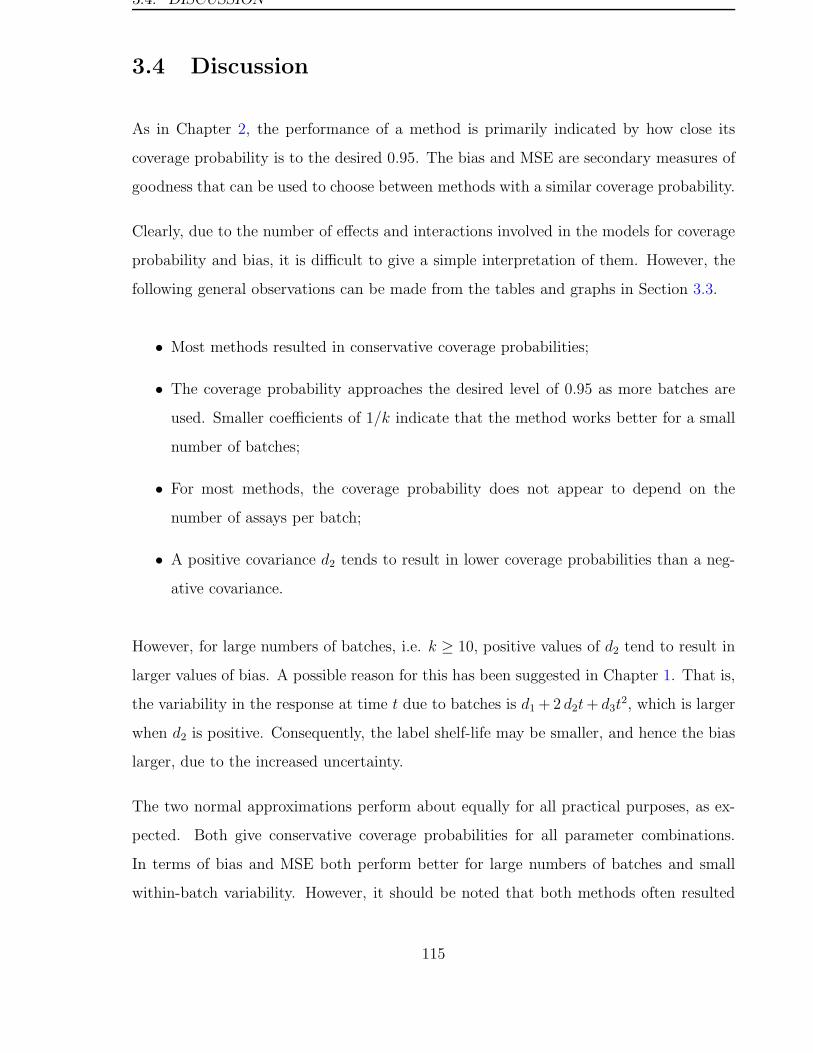
3.4. DISCUSSION
3.4 Discussion
As in Chapter 2, the performance of a method is primarily indicated by how close its
coverage probability is to the desired 0.95. The bias and MSE are secondary measures of
goodness that can be used to choose between methods with a similar coverage probability.
Clearly, due to the number of effects and interactions involved in the models for coverage
probability and bias, it is difficult to give a simple interpretation of them. However, the
following general observations can be made from the tables and graphs in Section 3.3.
• Most methods resulted in conservative coverage probabilities;
• The coverage probability approaches the desired level of 0.95 as more batches are
used. Smaller coefficients of 1/k indicate that the method works better for a small
number of batches;
• For most methods, the coverage probability does not appear to depend on the
number of assays per batch;
• A positive covariance d2 tends to result in lower coverage probabilities than a neg-
ative covariance.
However, for large numbers of batches, i.e. k ≥ 10, positive values of d2 tend to result in
larger values of bias. A possible reason for this has been suggested in Chapter 1. That is,
the variability in the response at time t due to batches is d1 + 2 d2t+ d3t2, which is larger
when d2 is positive. Consequently, the label shelf-life may be smaller, and hence the bias
larger, due to the increased uncertainty.
The two normal approximations perform about equally for all practical purposes, as ex-
pected. Both give conservative coverage probabilities for all parameter combinations.
In terms of bias and MSE both perform better for large numbers of batches and small
within-batch variability. However, it should be noted that both methods often resulted
115
3.4. DISCUSSION
in a zero shelf-life for small numbers of batches, and hence neither is of much practical
value.
The TMPL approach was also conservative for all parameter combinations. However, its
bias and MSE tended to be worse than the normal approaches when the within batch
variability was small.
The CPL approach was, except for the NCT1 approach, the only approach that fell short
of the desired coverage probability of 0.95. This approach also appears to be the only one
largely affected by the covariance d2 and the within batch variability σ.
The TMCPL performed the best of all these methods. It was conservative for small
numbers of batches, which is a good property, but approached the desired coverage of
0.95 as the number of batches increased. It also appears to be only slightly affected by
the covariance d2 and within batch variability σ — at least for the range of values used
for these parameters. Furthermore, the bias and MSE for this method were smaller than
most other methods, and both measures tended toward zero as the number of batches
increased.
The NCT1 approach had reasonable coverage probabilities for small values of σ, but
worked very badly for large values of σ. This is clearly because the approximation in
Section 3.2.4 does not work well for these cases. This tends to get worse as k and N
increase and for negative d2. This is as expected.
These observations are different from the findings by Shao and Chow (1994), who suggest
that this approach is conservative for large numbers of batches and large σ. Clearly, this
is because Shao and Chow use (3.18) as the definition for the true shelf-life in the batch
case, which is different to Definition 3.
The NCT2 approach was also conservative — much more so than TMCPL — across the
range of parameter values. Consequently, the bias and MSE were also larger.
In conclusion, in the multi-batch case, the recommended method for obtaining a label
shelf-life is the TMCPL method, followed by the NCT2. The normal approximations and
116

3.4. DISCUSSION
TMPL cannot be recommended due to their large bias and MSE, which is mainly due
to many of the shelf-lives being estimated as zero, while the CPL approach cannot be
recommended due to their low coverage probabilities. The NCT1 approach clearly offers
a reasonable solution for small values of σ, but should not be used for large values.
117
CHAPTER 4
Estimation of Shelf-Life:
The GLM Single Batch Case
4.1 Introduction
The ICH guidelines state that
“regression analysis is considered an appropriate approach to evaluating the
stability data for a quantitative attribute”
and that
“the nature of the degradation relationship will determine whether the data
should be transformed for linear regression analysis. Usually the relationship
can be represented by a linear, quadratic or cubic function on an arithmetic
or logarithmic scale”.
These statements implicitly assume that the residuals from fitting an appropriate model
are normally distributed. This assumption has been used extensively in the literature, as
well as in the development of the new definitions of shelf-life in Chapters 2 and 3.
118
4.1. INTRODUCTION
The relationship between potency and time depends on the order of the kinetics involved
in the degradation process. A linear relationship between potency and time is referred to
as a zero order kinetic relationship, while a linear relationship between the logarithm of
potency and time is referred to as a first order kinetic relationship (Jerne and Perry, 1956;
Kirkwood, 1977; Carstensen and Rhodes, 2000).
The possible requirement for a transformation of the response raises several questions: Is
a linear relationship between the response and time the most appropriate; does the as-
sumption of normality hold; and, in particular, is the assumption of constancy of variance
realistic? Rather than transforming the data, generalised linear models (GLMs) may offer
a more appropriate alternative (McCullagh and Nelder, 1989).
The link function used in GLMs allows for different relationships between the mean re-
sponse and the explanatory variables. Distributions other than the Normal can be fitted
and heteroscedasticity can be accommodated using mean-variance relationships. For ex-
ample, using the Gamma distribution, the variance of the response Y can depend on the
mean according to the relationship Var [Y ] ∝ E [Y ]2, and the mean can be allowed to
decay or grow exponentially. It is not difficult to imagine a process in which the response
increases or decreases over time in such a fashion. Such processes are not covered in the
existing literature on stability analysis, but they will be the focus of this chapter.
Assume that the assay result y is a realisation of the random variable Y , which has
a distribution that belongs to the exponential family of distributions. The probability
density function (pdf) of Y is
f(y;µ, φ) = exp
A
φ
[
y a(µ) − b(
a(µ))]
+ c(y, φ)
, (4.1)
where
• A is a prior known weight,
• φ > 0 is the dispersion parameter,
• the mean µ is generally a function of the covariates,
119
4.1. INTRODUCTION
• a = a(µ) is an increasing and invertible function of µ that does vary with the
observations and is independent of φ,
• b(a) = b(
a(µ))
does not vary with the observations and is independent of φ, and
• c(y, φ) is a function of the response and φ that does not involve µ.
Further assume that the linear predictor is η = xT β = l(µ) where l(·) is the link function.
Consequently, µ = l−1(η) = m(η), say.
It can be shown (McCullagh and Nelder, 1989) that
E [Y ] = µ =∂b
∂a
Var [Y ] = φV (µ) =φ
A
∂µ
∂a,
where V (µ) denotes the variance function which does not depend on the scale parameter
φ.
Assuming that the scale parameter does not depend on x, the probability density function
at time t is denoted by f(y;µt, φ). Similarly, the distribution function, which gives the
probability P (Y ≤ y) at time t, shall be denoted by F (y;µt, φ).
Similar to Chapter 2, interest lies in the time at which 100ε% of the drug product falls
below the specification limit. Hence, the following definition extends Definition 1 to the
exponential family of distributions.
Definition 5 Assume that the amount of active ingredient y at time t comes from a
distribution that belongs to the exponential family of distributions with pdf given in (4.1)
and mean µt. Then, the true shelf-life, denoted by τε, is the minimum time at which
100ε% of the drug product from the current batch has an activity level that is less than or
equal to the pre-determined specification limit κ, that is,
τε = inf
t : F (κ;µt, φ) ≤ ε
,
where F (·) denotes the distribution function of y.
120
4.2. LIKELIHOOD BASED APPROACHES
In Chapters 2 and 3 it was shown that the normal approximation to the lower ε quan-
tile was not very satisfactory. Since the parameters are not guaranteed to be normally
distributed, the normal approximation is even less likely to hold here. Furthermore, the
exact approach is no longer applicable for the same reason. However, a natural way to es-
timate parameters in the GLM setting is via likelihood methods. In general, β0 cannot be
eliminated via substitution, and consequently the basic profile likelihood will not provide
a workable approach. However the constrained profile likelihood gives a suitable approach
due to the simple penalizing of the likelihood function. This approach is investigated in
the next Section.
4.2 Likelihood based approaches
Let y = (y1, . . . , yN)T be a sample of the response with covariates xi1, . . . , xip correspond-
ing to the i-th response. Then, the joint log likelihood of the parameters β and φ, based
on (4.1), is given by
L(β, φ ;y) =
N∑
i=1
Ai
φ
yi ai − bi(ai)
+ c(yi, φ) .
The elements of the score are given by
∂L
∂βl
=N∑
i=1
Ai
φ
(
yi −∂bi∂ai
)∂ai
∂µi
∂µi
∂ηi
∂ηi
∂βl
=
N∑
i=1
Ai
φ
(yi − µi)∂ai
∂µi
∂µi
∂ηixil
∂L
∂φ=
N∑
i=1
−Ai
φ2
yi ai − bi(ai)
+∂ci∂φ
,
where ci = c(yi, φ). The score of βl can be written as
∂L
∂βl=
(
yi − µi
∂µi/∂ηi
)(
(∂µi/∂ηi)2
Var [ yi ]
)
xil = eiwixil .
Letting e = (e1, . . . , eN)T and W = diag(w1, . . . , wN), the score of β can be written as
∂L
∂β= XTWe .
121
4.2. LIKELIHOOD BASED APPROACHES
The elements of the observed information matrix are given by
Io(βl, βm) =N∑
i=1
Ai
φ
∂ai
∂µi
(
∂µi
∂ηi
)2
− (yi − µi)
[
∂2ai
∂µ2i
(
∂µi
∂ηi
)2
+∂ai
∂µi
∂2µi
∂η2i
]
xilxim
Io(βl, φ) =1
φ
∂L
∂βl
Io(φ, φ) =N∑
i=1
−2Ai
φ3
yi ai − bi(ai)
− ∂2ci∂φ2
,
and the elements of the expected information matrix are
Ie(βl, βm) =
N∑
i=1
Ai
φ
∂ai
∂µi
(
∂µi
∂ηi
)2
xilxim
Ie(βl, φ) = 0
Ie(φ, φ) =
N∑
i=1
−2Ai
φ3
µi ai − bi(ai)
− E
[
∂2ci∂φ2
]
.
Since Ie(β,β) = Var[
∂L∂β
]
and Var [ e ] = W−1 it follows that Ie(β,β) = XTWX.
Fisher scoring can then be used, with appropriate starting estimate, to find the maximum
likelihood estimates for β and φ.
4.2.1 Constrained Profile Likelihood
As in Chapter 2 the constrained estimates are found by minimizing the objective function
H(θτε ; τε,y) =1
N
[
−L(θτε)]
+ ω[
g(θτε ; τε) + ψ]2
, (4.2)
where θτε = (βTτε, φτε)
T , and g(θτε ; τε) can take the form
g(θτε; τε) = F (κ; βτε, φτε) − ε (4.3)
g(θτε; τε) = F−1(ε; βτε, φτε) − κ (4.4)
where F−1(·) denotes the inverse of F (·).
122

4.2. LIKELIHOOD BASED APPROACHES
The score vector now has components
∂H
∂βτε
=1
N
[
−XTWe]
+ 2ω[
g(θτε ; τε) + ψ] ∂g
∂βTτε
∂H
∂φτε
=1
N
[
−N∑
i=1
−Ai
φ2τε
yi ai + bi(ai)
+∂ci∂φτε
]
+ 2ω[
g(θτε ; τε) + ψ] ∂g
∂φTτε
.
Consequently, the components of the Powell-Hestenes equivalents of the observed infor-
mation matrix are given by
Io′(βτε
,βτε) =
1
N
[
XTWX]
+ 2ω( ∂g
∂βτε
)( ∂g
∂βTτε
)
Io′(βτε
, φτε) =1
N
[ 1
φτε
XTWe]
+ 2ω( ∂g
∂βτε
)( ∂g
∂φτε
)
Io′(φτε , φτε) =
1
N
[
N∑
i=1
−2Ai
φ3τε
yi ai − bi(ai)
− ∂2ci∂φ2
τε
]
+ 2ω( ∂2g
∂φ2τε
)
,
and the elements of the equivalent of the expected information matrix are
Ie′(βτε
,βτε) =
1
N
[
XTWX]
+ 2ω( ∂g
∂βτε
)( ∂g
∂βTτε
)
Ie′(βτε
, φτε) = 0 + 2ω( ∂g
∂βτε
)( ∂g
∂φτε
)
Ie′(φτε, φτε) =
1
N
[
N∑
i=1
−2Ai
φ3τε
µi ai − bi(ai)
− E
[
∂2ci∂φ2
τε
]
]
+ 2ω( ∂2g
∂φ2τε
)
.
The form of the score and information matrix now depend on the derivatives of g(·) which
are investigated below.
First, however, it is worthwhile to note that the modification of the constrained profile
likelihood developed in Chapter 2 can also be used here. The matrix C0 is obtained by
evaluating∂g
∂θTτε
=[
∂g∂β0,τε
∂g∂β1,τε
∂g∂φτε
]
at θτε = θτε.
123
4.2. LIKELIHOOD BASED APPROACHES
Derivative of g(θτε; τε) = F (κ; βτε, φτε) − ε
In this case, κ and ε are assumed fixed and differentiating g(θτε ; τε) with respect to βτε
gives∂g
∂βτε
=∂F (κ)
∂µτε
∂µτε
∂ητε
xτε , (4.5)
where F (κ) = F (κ; βτε, φτε) for notational simplicity. The second derivative on the right
hand side depends only on the link function, while the first element equals
∂F (κ)
∂µτε
=
∫ κ
−∞
∂f(z)
∂µτε
dz ,
where F (κ) = F (κ; βτε, φτε) and f(z) = f(z; βτε, φτε). This reduces to
∂F (κ)
∂µτε
=
∫ κ
−∞f(z)
z − µτε
φτεV (µτε)dz =
1
φτεV (µτε)
[
µτε(κ) − µτε
]
F (κ) , (4.6)
where µτε(κ) denotes the mean, given τε, of the distribution of Y , right truncated at κ.
Similarly, differentiating g(θτε; τε) with respect to φτε gives
∂g
∂φτε
=∂F (κ)
∂φτε
= M(κ;µτε , φτε)F (κ) , (4.7)
where
M(κ;µτε , φτε) = − A
φ2τε
[
µτε(κ)aτε − bτε
]
+
∫ κ
−∞
∂c(z, φτε)
∂φτε
f(z)
F (κ)dz
and aτε = a(µτε) and bτε = b(
a(µτε))
. Whether the integral can be calculated analytically
is unknown until the distribution, and hence the form of the pdf, is known.
Derivative of g(θτε; τε) = F−1(ε; βτε, φτε) − κ
As above, κ and ε are known and fixed in advance. However, at any given time τε the
value of F−1(ε) = F−1(ε; βτε, φτε) is not fixed as it depends on the value of the parameters.
Hence, let F−1(ε) = yτε(ε;µτε, φτε) = yτε, which is the ε quantile of the response at time
τε. Then F (yτε) can be differentiated using Leibniz’ Theorem, that is,
∂F (yτε)
∂µτε
=
[∫ yτε
−∞
∂f(z)
∂µτε
dz
]
+ f(yτε)∂yτε
∂µτε
=1
φτεV (µτε)
[
µτε(yτε) − µτε
]
F (yτε) + f(yτε)∂yτε
∂µτε
.
124
4.2. LIKELIHOOD BASED APPROACHES
However, since F (yτε) = ε is constant it follows that ∂F (yτε)/∂µτε = 0, and therefore
∂yτε
∂µτε
=∂F−1(ε)
∂µτε
= −
[
µτε
(
F−1(ε))
− µτε
]
φτεV (µτε)
ε
f(
F−1(ε)) . (4.8)
The derivative of the constraint with respect to µτε is then given by
∂g
∂µτε
=∂F−1(ε)
∂µτε
∂µτε
∂ητε
xτε (4.9)
Using the same argument, it can be shown that
∂g
∂φτε
=∂F−1(ε)
∂φτε
= −M(
F−1(ε), µτε , φτε
) ε
f(
F−1(ε)) , (4.10)
where
M(
F−1(ε), µτε, φτε
)
= − A
φ2τε
[
µτε
(
F−1(ε))
aτε − bτε
]
+
∫ F−1(ε)
−∞
∂c(z, φτε)
∂φτε
f(z)
εdz .
4.2.2 Example: The Normal Distribution
In this section the constrained likelihood is applied to normally distributed data. The
results can then be compared with the corresponding results in Chapter 2.
The likelihood, written in exponential family notation, is
L(β, φ ;y) =
N∑
i=1
1
φ
[
yiµi −µ2
i
2
]
− 1
2
[y2i
φ+ log 2π + logφ
]
,
where φ = σ2 is the scale parameter, Ai = 1, a(µi) = µi and bi(ai) = a2i /2 = µ2
i /2. Also,
the mean and variance are given by E [Yi ] = µi and Var [Yi ] = φ, such that the variance
function is simply V [µi] = 1. Possible choices for the link function are the identity, the
canonical link, the inverse and the log link.
The objective function, for a given τε, is
H(θτε ;y) =1
N
[
−L(θτε ;y)]
+ ω[
g(θτε ; τε) − ψ]2
,
where θTτε
= (βTτε, φτε) The general forms of the score vector and information matrices can
be obtained using the usual approach. Exact forms clearly depend on the choice of link
function and the constraint g(·).
125
4.2. LIKELIHOOD BASED APPROACHES
The elements of the score vector are now given by
∂H
∂βτε
= − 1
Nφτε
N∑
i=1
(yi − µi,τε)∂µi,τε
∂ηi,τε
xi + 2ω[
g(θτε ; τε) + ψ] ∂g
∂βτε
∂H
∂φτε
=1
N
[
N∑
i=1
1
φ2τε
(
yiµi,τε −µ2
i,τε
2
)
− y2i
2φ2τε
+1
2φτε
]
+ 2ω[
g(θτε ; τε) + ψ] ∂g
∂φτε
where µi,τε and ηi,τε denote the constrained mean and linear predictor corresponding to
the i-th observation, respectively.
The elements of the Powell-Hestenes equivalent of the observed information matrix are
Io′(βτε
,βτε) = − 1
Nφτε
N∑
i=1
(yi − µi,τε)∂2µi,τε
∂η2i,τε
−(
∂µi,τε
∂ηi,τε
)2
xixTi + 2ω
∂g
∂βτε
∂g
∂βTτε
Io′(βτε
, φτε) =1
Nφ2τε
N∑
i=1
(yi − µi,τε)∂µi,τε
∂ηi,τε
xi + 2ω∂g
∂βτε
∂g
∂φτε
Io′(φτε, φτε) =
1
N
[
N∑
i=1
2
φ3τε
(
µ2i,τε
2− yiµi,τε
)
+y2
i
φ3τε
− 1
2φ2τε
]
+ 2ω( ∂g
∂φτε
)2
.
Taking expectations gives the elements of the equivalent of the expected information
matrix, that is,
Ie′(βτε
,βτε) =
1
Nφτε
N∑
i=1
(
∂µi,τε
∂ηi,τε
)2
xixTi + 2ω
∂g
∂βτε
∂g
∂βTτε
Ie′(βτε
, φτε) = 0 + 2ω∂g
∂βτε
∂g
∂φτε
Ie′(φτε, φτε) =
1
2φ2τε
+ 2ω( ∂g
∂φτε
)2
.
The score vector and the equivalent of the expected information matrix can then be used
in Fisher scoring to obtain estimates for βτεand φτε for given values of τε. Evaluating the
likelihood at these constrained estimates gives the profile likelihood for τε, L(τε), and the
value of τε that maximises this profile likelihood is the maximum likelihood estimate of
the shelf-life, τε. The generalised likelihood ratio statistic is given by
w(τε) = 2(
L(τε) − L(τε))
,
126
4.2. LIKELIHOOD BASED APPROACHES
which is distributed approximately χ21. Consequently, the label shelf-life, based on the
100(1 − α)% lower confidence bound, is given by
τε,L(α) = inf
t : (t ≤ τε) &(
w(t) ≤ χ21,1−2α
)
. (4.11)
As elucidated previously, the exact values of the score vector and information matrices
rely partially on the form of the constraint. The two forms of constraint discussed in
Section 4.2.1 will now be applied to the normal case. Before doing so, note that both forms
involve the right truncated mean. Higher order moments of the truncated distribution
may also arise depending on the form of c(y, φ).
For the normal distribution, the mean of the normal distribution of Y , truncated at κ is
given by (Patel and Read, 1982)
µτε(κ) = µτε − φτε
f(κ)
F (κ),
and the variance is
σ2τε
(κ) = φτε(κ) = φτε
[
1 −(
κ− µτε
) f(κ)
F (κ)
]
−[
φτε
f(κ)
F (κ)
]2
.
Constraint 1: g(θτε ; τε) = F (κ; βτε, φτε) − ε
The derivative of the constraint with respect to βτεis
∂g
∂βτε
=1
φτε
[
µτε(κ) − µτε
]
F (κ)xτε = −f(κ)xτε .
Similarly, the derivative of the constraint with respect to φτε is given by
∂g
∂φτε
=F (κ)
φ2τε
µτε
[
µτε
2− µτε
]
+
∫ κ
−∞
[
t2
2φ2τε
− 1
2φτε
]
f(t) .dt
=F (κ)
φ2τε
µτε
[
µτε
2− µτε
]
+F (κ)
2φ2τε
[
στε(κ) + µ2τε
]
− F (κ)
2φτε
= −κ− µτε
2φτε
f(κ) .
127

4.2. LIKELIHOOD BASED APPROACHES
Constraint 2: g(θτε ; τε) = F−1(ε; βτε, φτε) − κ
The derivative of the constraint with respect to βτεis
∂g
∂βτε
= −
[
µτε
(
F−1(ε))
− µτε
]
ε
φτε f(
F−1(ε)) xτε = xτε .
Similarly, the derivative of the constraint with respect to φτε is given by
∂g
∂φτε
= −
− 1
φτε
[
µτε
(
F−1(ε))
µτε −µ2
τε
2
]
+
∫ F−1(ε)
−∞
[
z2
2φ2τε
− 1
2φτε
]
f(z)
ε.dz
ε
f(
F−1(ε))
= −
− µ2τε
2φ2τε
+µτε f
(
F−1(ε))
ε φτε
− 1
2φτε
+σ2
τε
(
F−1(ε))
2φ2τε
+µ2
τε
(
F−1(ε))
2φ2τε
+
ε
f(
F−1(ε)) ,
which reduces to∂g
∂φτε
=F−1(ε) − µτε
2φτε
.
Notice the closeness of both derivatives to the derivatives of Constraint 1. Also note that
this constraint is identical to the constraint used in Section 2.2.3.
4.2.3 Example: The Gamma Distribution
This section details the methods developed in Section 4.2.1 when applied to Gamma
distributed data.
There are various parameterizations of the Gamma distribution available. For sake of
consistency with (4.1), a modified form of the density used in McCullagh and Nelder
(1989) is chosen here.
Let Y have a gamma distribution with mean and scale parameters µ and φ, respectively.
This distribution is denoted by γ(µ, φ). The density of Y is given by
f(y) =y
1
φ−1e−
yφµ
(φµ)1
φ Γ(
1φ
)
. (4.12)
128

4.2. LIKELIHOOD BASED APPROACHES
Consequently, the joint log-likelihood, in exponential family notation, for a sample of size
N is given by
L(β, φ ;y) =
N∑
i=1
1
φ
− yi
µi− logµi
+
(1
φ− 1)
log yi −1
φlogφ− log Γ
(1
φ
)
where Γ denotes the gamma function (Abramowitz and Stegun 1972, (6.1.1)). Hence,
it follows that Ai = 1, ai(µi) = − 1µi
and bi(ai) = − log(−ai) = log µi. Furthermore,
E [Yi ] = µi and Var [Yi ] = φµ2i , and hence the variance function equals V (µi) = µ2
i .
Possible choices for the link function are the inverse, which is the canonical link, the log,
and the identity link.
As before, the objective function used to find the constrained maximum likelihood esti-
mates is given by (4.2), and the general forms of the Powell-Hestenes equivalents of the
score vector and information matrices can be found quite easily. However, the exact forms
depend on the choice of link function and form of constraint g(·).
The elements of the score vector are found as usual, that is,
∂H
∂βτε
= − 1
Nφτε
N∑
i=1
(
yi
µ2i,τε
− 1
µi,τε
)
∂µi,τε
∂ηi,τε
xi + 2ω[
g(θτε ; τε) + ψ] ∂g
∂βτε
∂H
∂φτε
= − 1
Nφ2τε
N∑
i=1
(
yi
µi,τε
+ log µi,τε − log yi
)
+N(log φτε − 1) +Nψ( 1
φτε
)
+ 2ω[
g(θτε ; τε) + ψ] ∂g
∂φτε
where µi,τε and ηi,τε again denote the constrained mean and linear predictor corresponding
to the i-th observation, respectively, and ψ(·) denotes the digamma function (Abramowitz and Stegun
1972, (6.3.1)).
The elements of the Powell-Hestenes equivalent of the observed information matrix are
then
Io′(βτε
,βτε) = − 1
Nφτε
N∑
i=1
(
1
µ2i,τε
− 2yi
µ3i,τε
)(
∂µi,τε
∂ηi,τε
)2
+
(
yi
µ2i,τε
− 1
µi,τε
)
∂2µi,τε
∂η2i,τε
xixTi + 2ω
∂g
∂βτε
∂g
∂βTτε
129
4.2. LIKELIHOOD BASED APPROACHES
Io′(βτε
, φτε) =1
Nφ2τε
N∑
i=1
(
yi
µ2i,τε
− 1
µi,τε
)
∂µi,τε
∂ηi,τε
xi + 2ω∂g
∂βτε
∂g
∂φτε
Io′(φτε , φτε) =
1
Nφ3τε
2
[
N∑
i=1
(
yi
µi,τε
+ logµi,τε − log yi
)
+N(log φτε − 1) +Nψ( 1
φτε
)
]
−N(
1 −ψ(1)
(
1φτε
)
φτε
)
+ 2ω( ∂g
∂φτε
)2
,
where ψ(1)(·) is the trigamma function, the first derivative of the digamma function
(Abramowitz and Stegun 1972, (6.3.1)), and the second derivatives of g(·) have been
ignored as before (Osborne, 2000).
Taking expectations, the equivalent of the expected information matrix is given by
Ie′(βτε
,βτε) =
1
Nφτε
N∑
i=1
1
µ2i,τε
(
∂µi,τε
∂ηi,τε
)2
xixTi + 2ω
∂g
∂βτε
∂g
∂βTτε
Ie′(βτε
, φτε) = 0 + 2ω∂g
∂βτε
∂g
∂φτε
Ie′(φτε, φτε) =
1
φ3τε
ψ(1)(
1φτε
)
φτε
− 1
+ 2ω( ∂g
∂φτε
)2
,
Specific results for the link functions are obtained by substituting the appropriate deriva-
tive for∂µi,τε
∂ηi,τε.
Before discussing the two forms of constraints, it will be beneficial to give results for the
left truncated mean for the gamma distribution.
The r-th moment of the left truncated gamma distribution is (Johnson et al., 1994a)
µ(r)τε
(κ) = (φτεµτε)rΓκ∗
(
1φτε
+ r)
Γκ∗
(
1φ
) ,
where κ∗ = κφτεµτε
and
Γx(α) =
∫ x
0
tα−1e−t.dt
denotes the incomplete gamma function (Johnson et al. 1994, (17.4)). Consequently, the
left truncated mean is given by
µτε(κ) = φτεµτε
Γκ∗
(
1φτε
+ 1)
Γκ∗
(
1φ
) . (4.13)
130

4.2. LIKELIHOOD BASED APPROACHES
Constraint 1: g(θτε ; τε) = F (κ; βτε, φτε) − ε
In order to calculate (4.5), the derivative of F (κ) is required. The general form of this
derivative is given by (4.6), which becomes here
∂F (κ)
∂µτε
=1
φτεµ2τε
[
φτεµτε
Γκ∗
(
1φτε
+ 1)
Γκ∗
(
1φτε
) − µτε
][
Γκ∗
(
1φτε
)
Γ(
1φτε
)
]
=φτεΓκ∗
(
1φτε
+ 1)
− Γκ∗
(
1φτε
)
φτεµτεΓ(
1φτε
) ,
since F (κ) = Γκ∗
(
1φτε
)
/Γ(
1φτε
)
. This form can further be simplified (Abramowitz and Stegun
1972, (6.5.22)), that is
∂F (κ)
∂µτε
= −(
µτεΓ(
1φτε
)
)−1(
κ
φτεµτε
)1
φτε
exp
(
− κ
φτεµτε
)
.
Hence, the derivative of the constraint with respect to βτεis given by
∂g
∂βτε
= −(
µτεΓ(
1φτε
)
)−1(
κ
φτεµτε
)1
φτε
exp
(
− κ
φτεµτε
)
∂µτε
∂ητε
xτε ,
with the exact form depending on the link function.
Similarly, the derivative of g(·) with respect to φτε is found by substituting the relevant
pieces into (4.7). This gives
∂g
∂φτε
=F (κ)
φ2τε
µτε(κ)
µτε
+ logµτε + log φτε − 1 + ψ(
1φτε
)
− 1
F (κ)
∫ κ
0
f(z) log(z) .dz
.
Unfortunately, there is no analytic solution for the integral. However, it can easily be
evaluated numerically. The exact value again depends on the choice of link function.
Constraint 2: g(θτε ; τε) = F−1(ε; βτε, φτε) − κ
In the gamma case (4.8) becomes
∂F−1(ε)
∂µτε
= − 1
φτεµτε
[
µτε(F−1)
µτε
− 1
]
ε
f(
F−1(ε)) .
This can now be substituted into (4.9) and an exact form can be determined for the
various choices of link function.
131
4.3. SIMULATION RESULTS
Similarly, the derivative of the constraint with respect to φτε is given by
∂g
∂φτε
= − ε
φ2τεf(F−1)
µτε(F−1)
µτε
+ log µτε + log φτε − 1 + ψ(
1φτε
)
− 1
ε
∫ F−1
0
f(z) log(z) .dz
,
where F−1 = F−1(ε). As in the previous section, the integral cannot be solved analytically,
but it can be evaluated numerically.
4.3 Simulation Results
As in previous chapters, a simulation study is used to evaluate the approaches pro-
posed in this chapter and the software used to perform these simulations was again R
(Ihaka and Gentleman, 1996). The simulations were run for normally and gamma dis-
tributed data. Both of these are further discussed in the following sections.
It should be noted that Constraint 1 is on a probability scale, which is generally much
smaller than the scale of the log-likelihood or objective function. Consequently, the Fisher
scoring scheme may have difficulty converging to the solution quickly. This was numeri-
cally confirmed and hence this form of constraint was not used in the simulations.
4.3.1 The Normal Distribution
The simulations were structured in the same way as those in Chapter 2. Furthermore,
in order to compare the result more directly with those of Chapter 2 the same simulated
data were used here. However, under the general GLM framework only the CPL and
TMCPL methods are available.
As expected, the label shelf-lives obtained with both methods described in this chapter
were identical to those obtained using the methods of Chapter 2. Consequently, as the
coverage probability, bias and MSE are identical to those previously tabulated, no tables
are given here, and the reader is referred to the tables and discussion in Chapter 2.
132
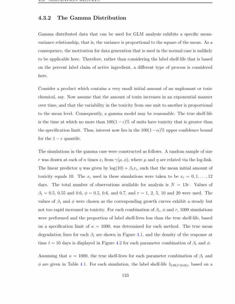
4.3. SIMULATION RESULTS
4.3.2 The Gamma Distribution
Gamma distributed data that can be used for GLM analysis exhibits a specific mean-
variance relationship, that is, the variance is proportional to the square of the mean. As a
consequence, the motivation for data generation that is used in the normal case is unlikely
to be applicable here. Therefore, rather than considering the label shelf-life that is based
on the percent label claim of active ingredient, a different type of process is considered
here.
Consider a product which contains a very small initial amount of an unpleasant or toxic
chemical, say. Now assume that the amount of toxin increases in an exponential manner
over time, and that the variability in the toxicity from one unit to another is proportional
to the mean level. Consequently, a gamma model may be reasonable. The true shelf-life
is the time at which no more than 100(1− ε)% of units have toxicity that is greater than
the specification limit. Thus, interest now lies in the 100(1−α)% upper confidence bound
for the 1 − ε quantile.
The simulations in the gamma case were constructed as follows. A random sample of size
r was drawn at each of n times xi from γ(µ, φ), where µ and η are related via the log-link.
The linear predictor η was given by log(10) + β1xi, such that the mean initial amount of
toxicity equals 10. The xi used in these simulations were taken to be xi = 0, 1, . . . , 12
days. The total number of observations available for analysis is N = 13r. Values of
β1 = 0.5, 0.55 and 0.6, φ = 0.5, 0.6, and 0.7, and r = 1, 2, 5, 10 and 20 were used. The
values of β1 and φ were chosen as the corresponding growth curves exhibit a steady but
not too rapid increased in toxicity. For each combination of β1, φ and r, 1000 simulations
were performed and the proportion of label shelf-lives less than the true shelf-life, based
on a specification limit of κ = 1000, was determined for each method. The true mean
degradation lines for each β1 are shown in Figure 4.1, and the density of the response at
time t = 10 days is displayed in Figure 4.2 for each parameter combination of β1 and φ.
Assuming that κ = 1000, the true shelf-lives for each parameter combination of β1 and
φ are given in Table 4.1. For each simulation, the label shelf-life τ0.99,U(0.05), based on a
133
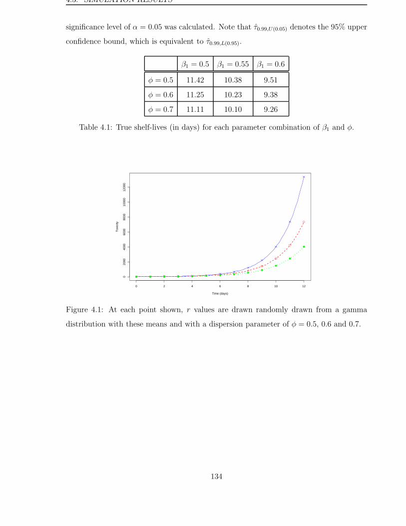
4.3. SIMULATION RESULTS
significance level of α = 0.05 was calculated. Note that τ0.99,U(0.05) denotes the 95% upper
confidence bound, which is equivalent to τ0.99,L(0.95).
β1 = 0.5 β1 = 0.55 β1 = 0.6
φ = 0.5 11.42 10.38 9.51
φ = 0.6 11.25 10.23 9.38
φ = 0.7 11.11 10.10 9.26
Table 4.1: True shelf-lives (in days) for each parameter combination of β1 and φ.
0 2 4 6 8 10 12
020
0040
0060
0080
0010
000
1200
0
Time (days)
Tox
icity
Figure 4.1: At each point shown, r values are drawn randomly drawn from a gamma
distribution with these means and with a dispersion parameter of φ = 0.5, 0.6 and 0.7.
134
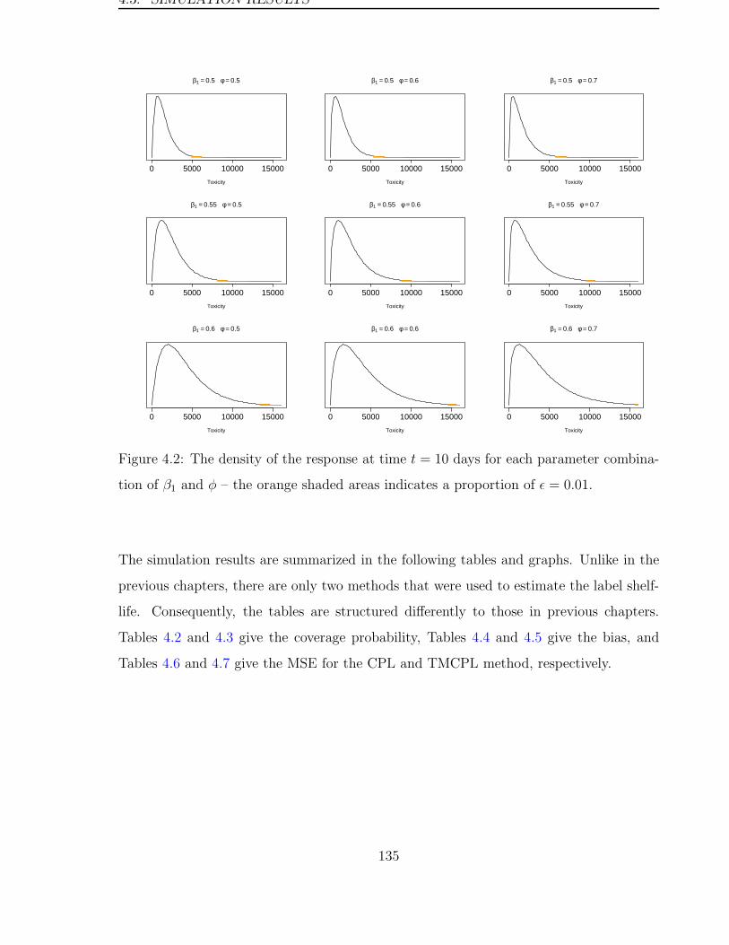
4.3. SIMULATION RESULTS
0 5000 10000 15000
β1 = 0.5 φ = 0.5
Toxicity
0 5000 10000 15000
β1 = 0.5 φ = 0.6
Toxicity
0 5000 10000 15000
β1 = 0.5 φ = 0.7
Toxicity
0 5000 10000 15000
β1 = 0.55 φ = 0.5
Toxicity
0 5000 10000 15000
β1 = 0.55 φ = 0.6
Toxicity
0 5000 10000 15000
β1 = 0.55 φ = 0.7
Toxicity
0 5000 10000 15000
β1 = 0.6 φ = 0.5
Toxicity
0 5000 10000 15000
β1 = 0.6 φ = 0.6
Toxicity
0 5000 10000 15000
β1 = 0.6 φ = 0.7
Toxicity
Figure 4.2: The density of the response at time t = 10 days for each parameter combina-
tion of β1 and φ – the orange shaded areas indicates a proportion of ε = 0.01.
The simulation results are summarized in the following tables and graphs. Unlike in the
previous chapters, there are only two methods that were used to estimate the label shelf-
life. Consequently, the tables are structured differently to those in previous chapters.
Tables 4.2 and 4.3 give the coverage probability, Tables 4.4 and 4.5 give the bias, and
Tables 4.6 and 4.7 give the MSE for the CPL and TMCPL method, respectively.
135
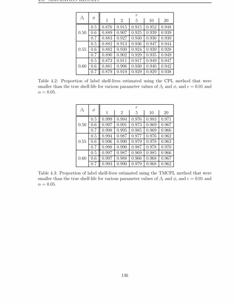
4.3. SIMULATION RESULTS
rβ1 φ
1 2 5 10 20
0.5 0.876 0.915 0.915 0.952 0.9480.50 0.6 0.889 0.907 0.925 0.939 0.939
0.7 0.883 0.927 0.930 0.930 0.9390.5 0.882 0.913 0.936 0.947 0.944
0.55 0.6 0.882 0.930 0.924 0.939 0.9280.7 0.890 0.902 0.929 0.935 0.9490.5 0.873 0.911 0.917 0.949 0.947
0.60 0.6 0.881 0.906 0.930 0.940 0.9420.7 0.879 0.919 0.929 0.929 0.938
Table 4.2: Proportion of label shelf-lives estimated using the CPL method that weresmaller than the true shelf-life for various parameter values of β1 and φ, and ε = 0.01 andα = 0.05.
rβ1 φ
1 2 5 10 20
0.5 0.999 0.994 0.976 0.983 0.9710.50 0.6 0.997 0.991 0.973 0.969 0.967
0.7 0.998 0.995 0.985 0.969 0.9660.5 0.994 0.987 0.977 0.976 0.962
0.55 0.6 0.996 0.990 0.979 0.978 0.9630.7 0.998 0.990 0.987 0.978 0.9700.5 0.997 0.987 0.969 0.985 0.966
0.60 0.6 0.997 0.988 0.966 0.968 0.9670.7 0.993 0.990 0.979 0.968 0.962
Table 4.3: Proportion of label shelf-lives estimated using the TMCPL method that weresmaller than the true shelf-life for various parameter values of β1 and φ, and ε = 0.01 andα = 0.05.
136
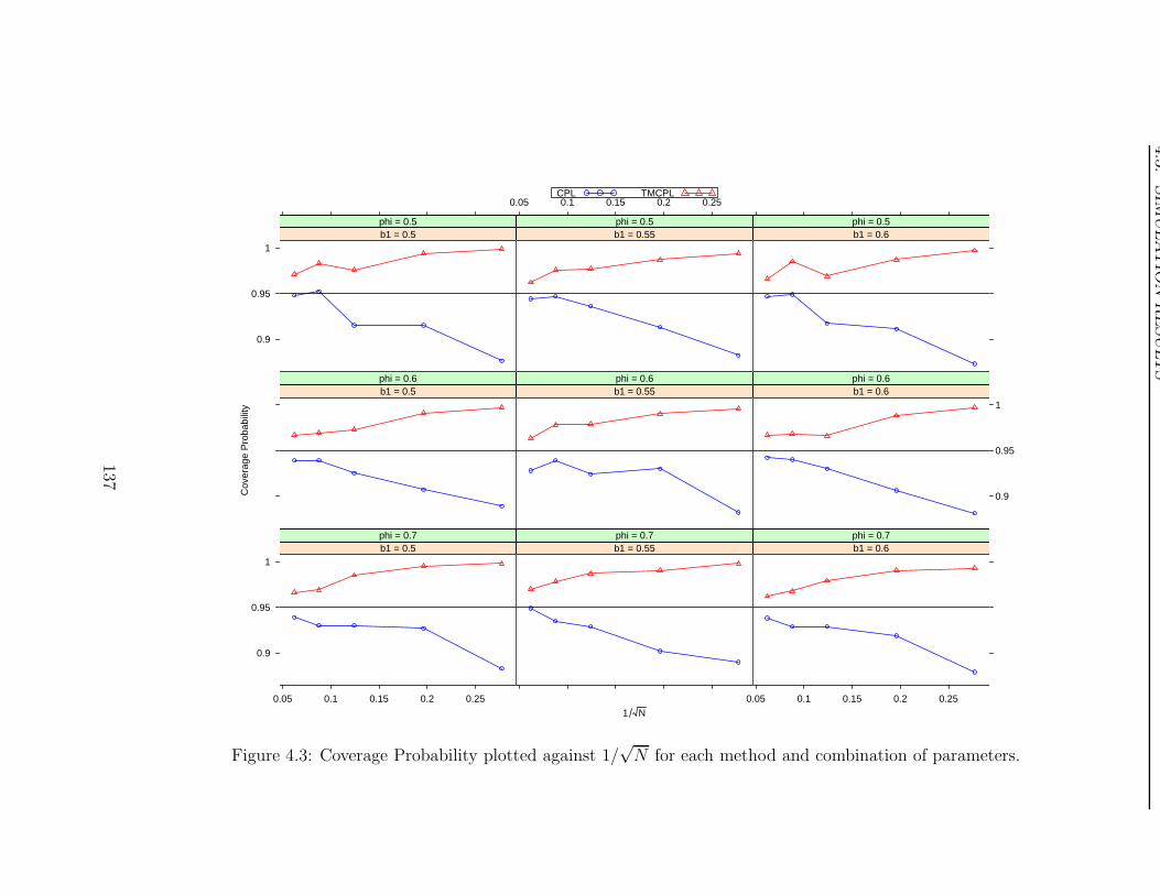
4.3
.SIM
ULA
TIO
NR
ESU
LT
S
1 N
Cov
erag
e P
roba
bilit
y
0.9
0.95
1b1 = 0.5phi = 0.5
b1 = 0.55phi = 0.5
0.05 0.1 0.15 0.2 0.25
b1 = 0.6phi = 0.5
b1 = 0.5phi = 0.6
b1 = 0.55phi = 0.6
0.9
0.95
1b1 = 0.6phi = 0.6
0.9
0.95
1
0.05 0.1 0.15 0.2 0.25
b1 = 0.5phi = 0.7
b1 = 0.55phi = 0.7
0.05 0.1 0.15 0.2 0.25
b1 = 0.6phi = 0.7
CPL TMCPL
Figure 4.3: Coverage Probability plotted against 1/√N for each method and combination of parameters.
137

4.3. SIMULATION RESULTS
rβ1 φ
1 2 5 10 20
0.5 −0.9 −0.7 −0.5 −0.4 −0.30.50 0.6 −1.0 −0.8 −0.6 −0.4 −0.3
0.7 −1.0 −0.8 −0.6 −0.4 −0.30.5 −0.8 −0.6 −0.4 −0.3 −0.2
0.55 0.6 −0.8 −0.7 −0.4 −0.3 −0.20.7 −0.9 −0.7 −0.5 −0.3 −0.20.5 −0.7 −0.5 −0.3 −0.3 −0.2
0.60 0.6 −0.7 −0.5 −0.4 −0.3 −0.20.7 −0.7 −0.6 −0.4 −0.3 −0.2
Table 4.4: Bias of label shelf-lives estimated using the CPL method for various parametervalues of β1 and φ, and ε = 0.01 and α = 0.05.
rβ1 φ
1 2 5 10 20
0.5 −2.5 −1.4 −0.7 −0.5 −0.30.50 0.6 −2.6 −1.5 −0.8 −0.5 −0.3
0.7 −2.8 −1.6 −0.8 −0.5 −0.40.5 −2.0 −1.1 −0.6 −0.4 −0.3
0.55 0.6 −2.1 −1.2 −0.6 −0.4 −0.30.7 −2.3 −1.2 −0.7 −0.4 −0.30.5 −1.6 −0.9 −0.5 −0.3 −0.2
0.60 0.6 −1.8 −0.9 −0.5 −0.3 −0.20.7 −1.9 −1.0 −0.5 −0.3 −0.2
Table 4.5: Bias of label shelf-lives estimated using the TMCPL method for various pa-rameter values of β1 and φ, and ε = 0.01 and α = 0.05.
138
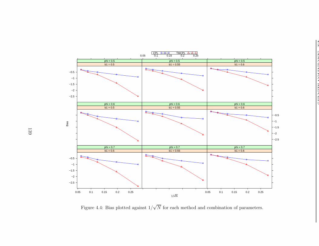
4.3
.SIM
ULA
TIO
NR
ESU
LT
S
1 N
Bia
s
−2.5
−2
−1.5
−1
−0.5
b1 = 0.5phi = 0.5
b1 = 0.55phi = 0.5
0.05 0.1 0.15 0.2 0.25
b1 = 0.6phi = 0.5
b1 = 0.5phi = 0.6
b1 = 0.55phi = 0.6
−2.5
−2
−1.5
−1
−0.5
b1 = 0.6phi = 0.6
−2.5
−2
−1.5
−1
−0.5
0.05 0.1 0.15 0.2 0.25
b1 = 0.5phi = 0.7
b1 = 0.55phi = 0.7
0.05 0.1 0.15 0.2 0.25
b1 = 0.6phi = 0.7
CPL TMCPL
Figure 4.4: Bias plotted against 1/√N for each method and combination of parameters.
139

4.3. SIMULATION RESULTS
rβ1 φ
1 2 5 10 20
0.5 1.5 0.8 0.4 0.2 0.10.50 0.6 1.6 0.9 0.4 0.2 0.1
0.7 1.8 1.0 0.4 0.2 0.10.5 1.1 0.6 0.2 0.1 0.1
0.55 0.6 1.1 0.7 0.3 0.1 0.10.7 1.3 0.7 0.3 0.2 0.10.5 0.8 0.4 0.2 0.1 0.0
0.60 0.6 0.8 0.4 0.2 0.1 0.10.7 0.9 0.5 0.2 0.1 0.1
Table 4.6: MSE of label shelf-lives estimated using the CPL method for various parametervalues of β1 and φ, and ε = 0.01 and α = 0.05.
rβ1 φ
1 2 5 10 20
0.5 6.9 2.2 0.6 0.3 0.10.50 0.6 7.5 2.4 0.7 0.3 0.1
0.7 8.4 2.7 0.8 0.3 0.20.5 4.4 1.4 0.4 0.2 0.1
0.55 0.6 4.8 1.6 0.5 0.2 0.10.7 6.0 1.7 0.5 0.2 0.10.5 2.9 0.9 0.3 0.1 0.1
0.60 0.6 4.0 1.0 0.3 0.1 0.10.7 5.2 1.2 0.3 0.2 0.1
Table 4.7: MSE of label shelf-lives estimated using the TMCPL method for various pa-rameter values of β1 and φ, and ε = 0.01 and α = 0.05.
140
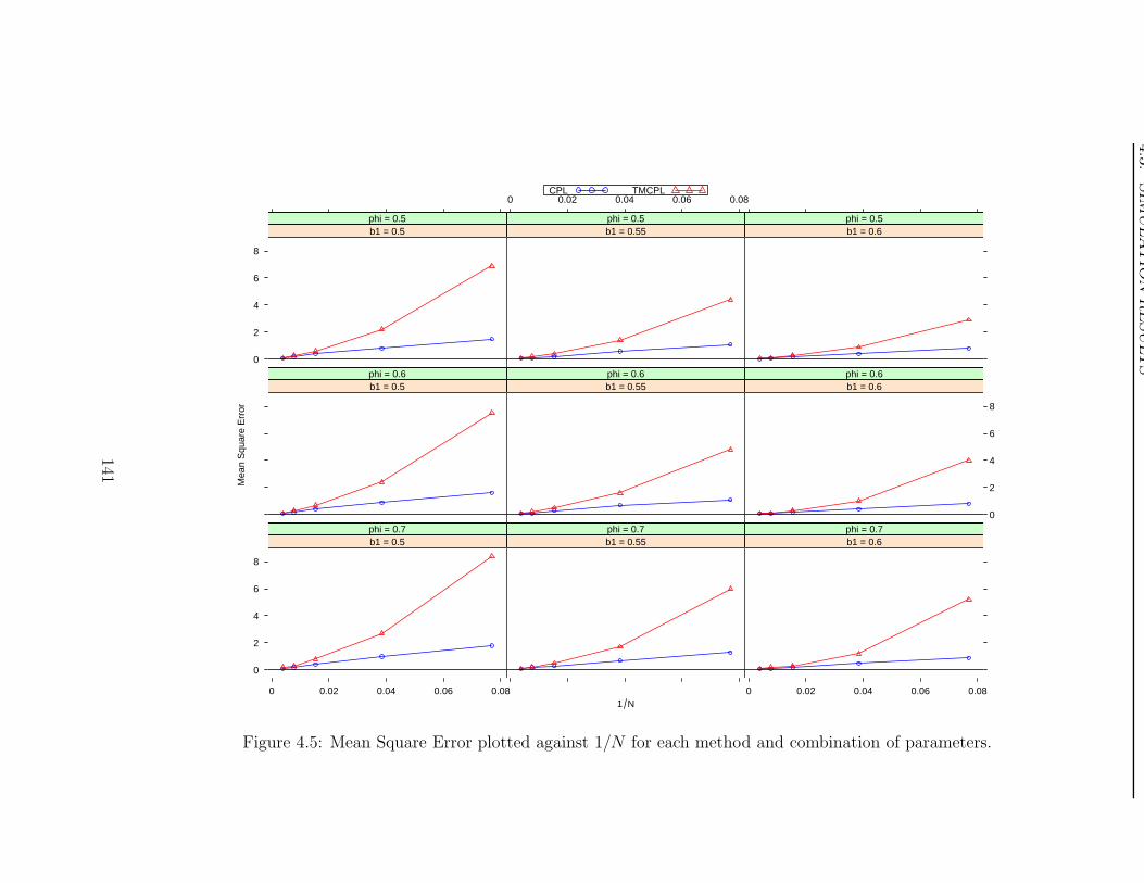
4.3
.SIM
ULA
TIO
NR
ESU
LT
S
1 N
Mea
n S
quar
e E
rror
0
2
4
6
8
b1 = 0.5phi = 0.5
b1 = 0.55phi = 0.5
0 0.02 0.04 0.06 0.08
b1 = 0.6phi = 0.5
b1 = 0.5phi = 0.6
b1 = 0.55phi = 0.6
0
2
4
6
8
b1 = 0.6phi = 0.6
0
2
4
6
8
0 0.02 0.04 0.06 0.08
b1 = 0.5phi = 0.7
b1 = 0.55phi = 0.7
0 0.02 0.04 0.06 0.08
b1 = 0.6phi = 0.7
CPL TMCPL
Figure 4.5: Mean Square Error plotted against 1/N for each method and combination of parameters.
141
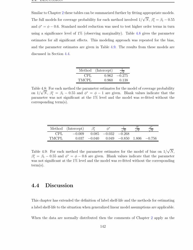
4.4. DISCUSSION
Similar to Chapter 2 these tables can be summarized further by fitting appropriate models.
The full models for coverage probability for each method involved 1/√N , β∗
1 = β1 − 0.55
and φ∗ = φ− 0.6. Standard model reduction was used to test higher order terms in turn
using a significance level of 1% (observing marginality). Table 4.8 gives the parameter
estimates for all significant effects. This modeling approach was repeated for the bias,
and the parameter estimates are given in Table 4.9. The results from these models are
discussed in Section 4.4.
Method (Intercept) 1√N
CPL 0.962 −0.275TMCPL 0.960 0.138
Table 4.8: For each method the parameter estimates for the model of coverage probabilityon 1/
√N , β∗
1 = β1 − 0.55 and φ∗ = φ − 1 are given. Blank values indicate that theparameter was not significant at the 1% level and the model was re-fitted without thecorresponding term(s).
Method (Intercept) β∗1 φ∗ 1√
N
β∗
1√N
φ∗
√N
CPL −0.009 0.085 −0.032 −0.268TMCPL 0.037 −0.040 0.049 −0.850 1.806 −0.756
Table 4.9: For each method the parameter estimates for the model of bias on 1/√N ,
β∗1 = β1 − 0.55 and φ∗ = φ − 0.6 are given. Blank values indicate that the parameter
was not significant at the 1% level and the model was re-fitted without the correspondingterm(s).
4.4 Discussion
This chapter has extended the definition of label shelf-life and the methods for estimating
a label shelf-life to the situation when generalized linear model assumptions are applicable.
When the data are normally distributed then the comments of Chapter 2 apply as the
142
4.4. DISCUSSION
GLM based methods result in the same shelf-life as the corresponding methods in Chap-
ter 2.
In the gamma case, the CPL method tends to give coverage probabilities that fall short of
the desired 0.95 for small N , but it does tend toward 0.95 as N → ∞. This is analogous
to the observations made for the normal distribution in Chapter 2. However, the rate at
which the coverage probability approaches 0.95 does appear to only depend on N . While
this is different to the observations made in Chapter 2, this may be due to the choice
of values for β1 and φ that were used in the simulations. In addition, the bias of the
CPL method also tends to be relatively small when compared to the bias of the TMCPL
method. This is not surprising as the CPL tends to give coverage probabilities that fall
short of the desired 0.95.
The TMCPL in the gamma case results in conservative coverage probabilities, as in the
normal case, but here it appears to remain conservative for large N . Similar to Chapter 2,
the rate at which the coverage probability approaches 0.95 depends only on the sample
size N . The bias on the other hand appears to depend on N , β1 and φ, which is analogous
to the observations made in Chapter 2.
In conclusion, the TMCPL can also be recommended in the GLM case, as the coverage
probabilities obtain from this method tend to be conservative, but close to the desired
level of 0.95. The CPL can only be recommended for very large sample size.
143
CHAPTER 5
Conclusions
Several issues have been raised in Chapter 1 in relation to the design of stability trials
and the analysis of stability data as currently outlined in the regulatory guidelines.
The current frequency and spacing of time points at which the product is assayed have
been shown to be less than optimal. Consequently, it is suggested that the product
be sampled more frequently near the shelf-life, instead of being sampled more frequently
during the first year after manufacture. This has been shown to have immediate effects on
the accuracy of the estimated shelf-life and thus can extend the label shelf-life. However,
to sample very infrequently in the first year is of limited practical value as it is recognized
that estimates of the label shelf-life are usually desirable early in the life of a drug product.
Consequently, it is recommended that the product be assayed at equal time intervals
throughout its life, instead of less frequently during the second and consecutive years of
storage.
In respect to the assay result, the current guidelines assume that assay variability is the
only source of variability affecting the assay result. However, this thesis argues that the
variability in the drug product needs to be taken into account when determining a label
shelf-life. The only way these sources of variation can be distinguished is by duplicating
the assays at each time point. Assuming that the variability of the drug product can be
identified, new precise definitions for the true and label shelf-life are suggested.
144
5.1. OTHER APPLICATIONS
Another source of variability is due to batches. The current regulatory guidelines treat
batches as fixed effects, which does not allow conclusions to be drawn about future batches.
Assuming that batches are random effects has led many authors to develop statistical tests
which can be used to test whether the intercept and slope have a non-zero variance and
covariance, or whether they can be treated as fixed for all batches. It is pointed out
here that basing the estimation on a test of significance has some inherent problems.
Consequently, it is suggested that no such test be used, but that instead the model
appropriately account for batch-to-batch variability.
Based on the new definitions for true shelf-life, several methods for determining a label
shelf-life have been investigated. The results from simulation studies have shown that the
truncated modified profile likelihood approach is the most suitable under a variety of cir-
cumstances, including cases where batch-to-batch variability or non-normally distributed
data are present. Consequently, this method should be used in all situations except the
most simple — linear regression. In this situation the non-central t-distribution provides
an optimal solution.
While this thesis has mainly focused on the definition and estimation of a label shelf-
life in the pharmaceutical industry, the methods developed here are not limited to this
application. The following section gives some examples of where the use of the tolerance
bound as suggested in this thesis may be useful.
5.1 Other Applications
This thesis is primarily concerned with estimating a lower 100(1−α)% confidence bound
for the time at which a proportion ε of product first falls below the specification limit.
There are however, many more similar circumstances in which the new definitions and
associated method of estimation can be useful. Some applications which come to mind
are the following.
• Toxicity of a drug product: Some drug products may increase in toxicity over time.
145
5.1. OTHER APPLICATIONS
The manufacturer may be interested in estimating the time at which the 95% upper
confidence bound for the 0.99 quantile reaches the specification limit set for safe
consumption.
• Safety of food products: This scenario is very similar to the toxicity of drug products
(c.f. Section 4.2.3).
• Grow-out periods of farmed fish species: Fish species may accumulate chemical
residues during the time they are commercially farmed. Consequently, the producer
may be interested in the time at which he can be 90% confident that no more than
5% of fish have a residue level greater than some pre-determined limit. In this case,
animals may correspond to the batches, while herds may add yet another source of
variation not yet investigated.
• Withholding periods: Drugs and antibiotics can often be detected in the meat, milk,
etc. of farmed animals after being administered. The levels found in the produce
generally degrade over time. The withholding period is the time period for which
the produce should not be consumed (by humans) after the drug is administered.
This withholding period would require the estimation of the time at which no more
than 1% of animals show a residue level of more than the Maximum Residue Level
(MRL) with 95% confidence.
• Fuel tanks in cars: The distance that can be travelled by car with a single tank of
fuel will depend on many factors, including driver, size of fuel tank and probably
others. Drivers are likely to be random effects, similar to batches, while the size
of the fuel tank can be assumed to be the determining variable. Consequently, it
should be possible to determine the size of fuel tank that would be required such that
at most 5% of trips fall short of a desired target with 95% confidence. (While this
example is clearly fabricated, it illustrates the potential for the approach detailed
in this thesis).
146

5.2. FUTURE WORK
5.2 Future Work
While this thesis has addressed the issues indicated in Chapter 1, it has also raised many
more which will require further research. These include, but are not limited to, the
following questions which are listed in no particular order.
• It has been assumed that assay-to assay variability is either negligible or has been
eliminated by taking assay averages, for example. How can assay variability be
included in the modeling process?
• It has previously been mentioned that there are several possible sources of variability.
One such source, which has been assumed to be negligible, is day-to-day variability.
The question that arises is how such a source of variability can be included formally
in the analysis? This is particularly of interest when batches are put on stability
trials at different times, but are analysed at the same time. This situation is depicted
in Figure 5.1.
• How do β1, σ and d2 interact in the batch case? More simulations are required here.
• Random effects models in the GLM framework can already be fitted, but how can
the methods of Chapter 4 be generalised to the batch case? There is already an
extensive literature on fitting generalised linear mixed models (GLMM), e.g. Schall
(1991). However, these methods are approximate, and “efficient ways to fit GLMMs
are a research topic” (Venables and Ripley, 2002).
• Accelerated stability testing is a common approach to obtain estimates of the shelf-
life sooner. How do the methods presented in this thesis generalise to the nonlinear
models which are used in accelerated testing?
• How do the methods presented in this thesis perform when fractional factorial de-
signs are used in the stability trial?
• Can non-parametric quantile regression methods (Koenker and Bassett Jr, 1978) be
used in a similar way to those of Chapter 2, and can they be extended to the batch
147

5.2. FUTURE WORK
case? How do these non-parametric methods compare to the methods presented
here?
• The non-normal approximations have been shown to be poor. Why is this the case?
Is it because under the approximation the quantile qt,ε and its variance Var [ qt,ε ] are
not really independent? Can this be remedied (easily)?
• Poisson count data may arise when observing the growth of pathogens in food
products over time, e.g. Salmonella. How do the approaches in Chapter 4 perform
under Poisson assumptions? Can the methods of Chapter 4.1 be generalised to other
distributions?
• Bootstrap methods are often useful to estimate quantiles and their confidence bounds?
How do various bootstrap confidence intervals perform in the determination of a la-
bel shelf-life?
• How do the TMCPL and other methods behave for different values of ε and α?
Time
Batch 1
1 2 3 4 5 ...
Batch 2
Batch 3
Figure 5.1: Illustration of a stability trial design where batches are added to the trial over
time. At any particular point in time all batches are assayed.
148
Bibliography
Abramowitz, M. and I. A. Stegun. 1972. Handbook of mathematical functions , 9th ed., Dover.
Barndorff-Nielsen, O. 1983. On a formula for the distribution of the maximum likelihood estimator ,
Biometrika 70, 343–365.
Barron, A. M. 1994. Use of fractional factorial (or ’matrix’) designs in stability analysis, ASA Proceedings
of the Biopharmaceutical Section, pp. 475–481.
Buncher, C. R. and J.-Y. Tsay. 1993. 21a stability of drugs: Room temperature tests, Statistics in the
Pharmaceutical Industry, 2nd ed., Marcel Dekker (New York), pp. 419–444.
Carstensen, J. T. and E. Nelson. 1976. Terminology regarding labeled and contained amounts in dosage
forms , Journal of Pharmaceutical Sciences 65, 311–312.
Carstensen, J. T. and C. T. Rhodes. 2000. Drug stability: principles and practices, 3rd ed., Marcel Dekker,
New York.
Carter, R. L. and M. C. K. Yang. 1986. Large sample inference in random coefficient regression models ,
Communications in Statistics, Part A – Theory and Methods, 2507–2525.
Chen, J. J., J.-S. Hwang, and Y. Tsong. 1995. Estimation of the shelf-life of drugs with mixed effects
models , Journal of Biopharmaceutical Statistics 51, 131–140.
Chow, S.-C. and J.-P. Liu. 1995b. Statistical design and analysis in pharmaceutical sciences , Marcel
Dekker, Chapter 11 - Stability analysis with fixed batches Chapter 12 - Stability analysis with random
batches.
Chow, S.-C. and A. P. Pong. 1995a. Current issues in regulatory requirements of drug stability, Journal
of Food and Drug Analysis 3, 75–85.
Chow, S.-C. and J. Shao. 1989. Test for batch-to-batch variation in stability analysis, Statistics in Medicine
8, 883–890.
. 1990. Estimating drug shelf-life in NDA stability studies, ASA Proceedings of the Biopharma-
ceutical Section, The American Statistical Association, pp. 190–195.
149
BIBLIOGRAPHY
. 1991. Estimating drug shelf-life with random batches, Biometrics 47, 1071–1079.
Chow, S.-C. and S. G. Wang. 1994. On the estimation of variance-components in stability analysis ,
Communications in Statistics-Theory and Methods 23, 289–303.
Cox, D. R. and N. Reid. 1987. Parameter orthogonality and approximate conditional inference (with
discussion), Journal of the Royal Statistical Society - Series B 49, 1–39.
Easterling, R. G. 1969. Discrimination intervals for percentiles in regression, Journal of the American
Statistical Association 64, 1031–1041.
Freeman, P. R. 1989. The performance of the two-stage analysis of two-treatment, two period crossover
trials , Statistics in Medicine 8, 1421–1432.
Hinkley, D. V., N. Reid, and E. J. Snell. 1991. Statistical theory and modelling, Chapman and Hall.
Ho, C.-H., J.-P. Liu, and S.-C. Chow. 1992. On analysis of stability data., ASA Proceedings of the
Biopharmaceutical Section, American Statistical Association, pp. 198–203.
ICH. 2002. Evaluation of stability data (Q1E, Step 2), International Conference on Harmonisation of
Technical Requirements for Registration of Pharmaceuticals for Human Use.
. 2003. Stability testing of new drug substances and products (Q1A(R2), step 4 , International Con-
ference on Harmonisation of Technical Requirements for Registration of Pharmaceuticals for Human
Use.
Ihaka, R. and R. Gentleman. 1996. R: A language for data analysis and graphics , Journal of Computa-
tional and Graphical Statistics 5, 299–314.
Jerne, N. K. and W. L. M. Perry. 1956. The stability of biological standards, Bulletin of the World health
Organisation 14, 167–182.
Johnson, N. L., S. Kotz, and N. Balakrishnan. 1994a. Continuous univariate distributions, 2nd ed., vol. 1,
John Wiley and Sons Inc.
Ju, H. L. and S.-C. Chow. 1995. On stability designs in drug shelf-life estimation, Journal of Biopharma-
ceutical Statistics 5, 201–214.
Kiermeier, A., R. G. Jarrett, and A. P. Verbyla. 2004. A new approach to estimating shelf-life, Pharma-
ceutical Statistics (Accepted for publication).
Kirkwood, T. B. L. 1977. Predicting the stability of biological standards and products , Biometrics 33,
736–742.
Koenker, R. and G. Bassett Jr. 1978. Regression quantiles , Econometrica 46, 33–50.
Kohberger, R. C. 1988. Manufacturing and quality control , Biopharmaceutical Statistics for Drug Devel-
opment (K. E. . Peace, ed.), Marcel Dekker, New York, pp. 605–629.
150
BIBLIOGRAPHY
Lee, K. R. and R. C Cagon. 1994. Calibration and stability analysis with a simple mixed linear model when
the experiment is of a split-plot type, ASA Proceedings of the Biopharmaceutical Section, pp. 435–440.
Lin, K. K. 1990. Statistical analysis of stability study data, ASA Proceedings of the Biopharmaceutical
Section, The Americal Statistical Association, pp. 210–215.
Lu, C. J. and W. Q. Meeker. 1993. Using degradation measures to estimate a time-to-failure distribution,
Technometrics 35, 161–174.
McCullagh, P. and J. A. Nelder. 1989. Generalized linear models, 2nd ed., Chapman and Hall.
Nordbrock, E. 1992. Statistical comparison of stability study designs, Journal of Biopharmaceutical Statis-
tics 2, 91–113.
. 1994. Design and analysis of stability studies, ASA Proceedings of the Biopharmaceutical Section,
pp. 291–294.
Norwood, T. E. 1986. Statistical analysis of pharmaceutical stability data, Drug Developments and In-
dustrial Pharmacy 12, 553–560.
Osborne, M. R. 2000. Scoring with constraints , Australian & New Zealand Industrial and Applied Math-
ematics Journal 42, 9–25.
Patel, J. K. and C. B. Read. 1982. Handbook of the normal distribution, Marcel Dekker.
Ruberg, S. J. and J. C. Hsu. 1990. Multiple comparison procedures for pooling batches in stability study,
ASA Proceedings of the Biopharmaceutical Section, pp. 204–209.
. 1992. Multiple comparison procedures for pooling batches in stability study, Technometrics 34,
465–472.
Ruberg, S. J. and J. W. Stegeman. 1991. Pooling data for stability studies: Testing the equality of batch
degradation slopes , Biometrics 47, 1059–1069.
Satterthwaite, F. E. 1946. An approximate distribution of estimates of variance components., Biometric
Bulletin 2, 110–114.
Schall, R. 1991. Estimation in generalized linear models with random effects , Biometrika 78, 719–727.
Shao, J. and S.-C. Chow. 1994. Statistical inference in stability analysis, Biometrics 50, 753–763.
. 2001a. Drug shelf-life estimation, Statistica Sinica 11, 737–745.
Stead, A. G., S. B. Wilkins, and K. G. MacDonald. 1994. Using fractional factorial designs to improve
product shelf life, Proceedings of the Sas Users Group International Conference, vol. 19, SAS Institute,
pp. 980–983.
Sun, Y., S.-C. Chow, G. Li, and K.-W. Chen. 1999. Assessing distributions of estimated drug shelf lives
in stability analysis, Biometrics 55, 896–899.
151

BIBLIOGRAPHY
Tapon, R. 1993. Estimating shelf-life using l1 regression methods , Journal of Pharmaceutical and Biomed-
ical Analysis 11, 843–845.
Tatke, J. V. 1980. A statistical approach to shelf life characteristics of antibiotic bulk , Journal of the
Indian Statistical Association 18, 153–161.
Venables, W. N. and B. D. Ripley. 2002. Modern applied statistics with S, 4th ed., Statistics and Com-
puting, Springer-Verlag, New York.
Yoshioka, S., Y. Aso, S. Kojima, and N. F. Cappuccino. 2002. A comparison of the analysis of covari-
ance (ancova) and range-based approaches for assessing batch-to-batch variability of the stability of
pharmaceutical products , Chemical & Pharmaceutical Bulletin 50, 881–883.
152

Appendix A
The following paper has been accepted for publication in Pharmaceutical Statistics vol 3, 2004 pp: 3-11 Andreas Kiermeier, Richard G.Jarrett and Arunas P.Verbyla A new approach to estimating shelf life.
NOTE: This publication is included in the print copy of the thesis.
It is also available online to authorised users at:
http://dx.doi.org/10.1002/pst.78
A new approach to estimating shelf-lifeThis is a preprint of ui i"ti"l" published in Pha¡maceutical Statistics, 2004, 3, 3-11
http : / /www.interscience.wiley. com/
Andreas KiermeiertThe University of Adelaide/
SARDI
Arunas P. VerbylaThe University of Adelaide/
SARDI
24 J:¿ne 2003
Abstract
The current approach to the estimation of shelf-life and the determination
of the label shelf-life as detailed in the IcH guidelines to industry is presented'
sizes are made.
Keywords: stability Analysis, shelflife, Quantile, constraint, Modified
Profile Likelihood
1 Introduction
Pharmaceutical companies are required by law to indicate the expiry date of each
pharmaceutical product on the immediate container' This expiry date indicates
the end of the period of time, known as shelf-life, during which the product can
be expected to meet specifications. The guidelines which goveln how the label
iAuthor to whom correspondence should be addressed: BiometricsSA, PMB 1' Glen Osmond,
SA 5064, Australia, e-mail: Andreas.Kiermeier@adelaide'edu'au,Phone: +61 8 8303 6819, Facsimile: *61 8 8303 6761
Richard G. JarrettCSIRO
1

shelf-life, and hence the expiry date' is determined are set out by the International
Conference on Harmonisation (ICH) of Technical Requirements for Registration of
Pharmaceuticals for Human Use ([t], [Z]).
The ICH states thaL "usually the relationshi,p [between the sampli'ng ti'me and
assay resultl can be represented, by a linear, quad,ratic or cub'ic function on an arith-
metic or logari,thmic scale". An appropriate statistical model for such a relationship
might take the form
a¿:þ*e¿, (1)
where 3r¿ is the response from the z-th assay fot i : 1, . . . ,.1ú, on the arithmetic
or logarithmic scale, x¿ is a p-dimensional predictor vector corresponding to the
i-th response, p is a p-dimensional vector of fixed effects, and e¿ are independently
and identically distributed normal errors, with mean 0 and variance o2 ' In matrix
notation (1) can be exPressed as
y:XP+e,
where X is the design matrix with ¿-th row xfl. Variation can arise from two sources'
In this paper we are concerned with the unit-to-uni,ú variability, as exemplified by the
variation in the level of active ingredient from one tablet to another, say' A second
source is the variability associated with the measurement or assay system' We will
suppose that either this is small relativeto o2 or that it is separately estimated and
eliminated from the estimate of o2.
The current definition of sh'elf-li'fe ([1]) it
"the time interaal that a d,rug product is erpected to remain wi'thin the
2

g,pproued, shetf-life spec,ification prouided that it i,s stored under th'e con-
d,i,ti,ons d,efined, on the label i,n the proposed containers and clos'u,re."
Assuming that the response decreases over time, this deflnition is equivalent to the
mathematical definition for the true sltelf-Ii.fe of a single batch ([3]), namely the time
r such that
r-:inf t:x(t)rB<n, (2)
where inl denotes the infimum or greatest lower bound, rc is the specifi,cation limit
(or acceptance criterion) and x(t) is the vector of regressors at time ú' A similar
definition applies to responses that increase with time'
The guidelines also stipulate that the approach for determining the label shelf-li'fe
,,to d,etermine the time at whi,ch the 95% one-si,ded confid,ence limit for
the mean curae intersects the acceptance criterion" '
This approach attempts to give an assurance that the label shelf-life is smaller than
the true shelf-life with probability 1 - a. Hence, the label shelf-life is a 100(1 - o)%
lower confidence bound for the true shelf-life'
consequently, the tabet sttetf-tife, î¡6¡, is given by the time at which the lower
confidence bound for x(t)r B intersects the specifrcation limit ([4]),
1S
rLþ¿) : inf t : xl)r þ t to,¡,t-ps x(¿ T xrX)-rx(t) < o)
where to,N-p is the a quantile of the ú-distribution with N - p degrees of freedom,
and ¡â and s are the least squares estimates of B and o'
3

A different approach, which is based on the prediction interval of a future obser-
vation, ,ù/as proposed in [5]. They define what will be referred to as a modif'ed label
shetf-tife, given by the intersection of the 100(1 - d)% Iower prediction bound and
the specification limit, that is, the smallest value of t for which
*(t)'p * úa,ry-rs 1+ x(t)" ¡¡_r*(¿) ( rc (3)
This approach attempts to make a statement about the ability of an individual unit
(a tablet, say) to meet the specifications at time f, rather than the abilitv of the
mean of all units of the batch to meet the specifications'
Which defrnition is used clearly has important implications for the consumer.
The implications and problems with the current methodology will be discussed
in Section 2. This leads to a new formal definition of true shelf-life which addresses
these problems. In Section 3 several approaches are given that provide an estimate
of the label shelf-life corresponding to this new definition. These approaches are
evaluated in a simulation study presented in Section 4' A discussion of the results
and an indication of further work is given in Section 5'
2 An assessment of the various definitions
The current definition of the true shelf-llfe, r, as given in (2), is based on the line of
best fi.t. The esti,mated, shetf-ti,fe, î, is given by the intersection of the mean response
and the specification limit, i.e. it satisfies
î:inf t:x(t)rþa" .
The use of the lower confidence bound for the mean response yields the label shelf-
life, which is a lower confidence bound for the true shelf-life' As the sample size
4
increases the estimated shelf-life is determined more accurately. In the limiting case
as .lú --+ oo the label shelf-life approaches the true shelf-life. However, in the limit,
only 50% of the product remains within specification at time â.
If the unit-to-unit variability, a, is small, this may not be a problem since the
specification limit will not have been breached by a large amount' However, if a is
Iarge, some products may fall far short of the specification, with potentially serious
consequences
Another undesirable property of the current regulatory approach is the lack
of influence the product variability has on the estimation process. Increasing the
number of samples can compensate for a manufacturing process with large variability
ø. This is often cheaper than attempting to improve the manufacturing process, but
it does not put enough emphasis on good manufacturing practices and commitment
to quality.
On the other hand, the modified label shelf-life does not approach the true shelf-
Iife in large samples, but instead has the large sample property that ensures that a
proportion a of the drug product falls below the specification limit at the time the
modified label shelf-life has expired. This follows from the fact that as -fy' ---+ oo,
equation (3) reduces to
*(t)'Plzoo1n,
where the left hand side is the a quantile of the distribution of Y given x(t), and z"
is the a quantile of the standard normal distribution. We believe this to be a more
appropriate basìs for the true shelf-life'
To overcome the problenis with the current regulatory approach and the pre-
5

diction bound approach, the following new definitions of true shelf-life, estimated
shelf-life and label shelf-life are proposed.
Definition L und,er mod,el (7), the true shelf-life, denoted, by r,, is the m'ini'mum
ti,me at wh¿ch l00e% of the d,rug prod,uct from the current batch lt'as an actiui,ty Leuel
that i,s less than or equal to the pre-determi,ned speci,ficat'ion limi't n, that is,
r,: ilf- t : x(t)r B I z,o < rc ,
where *(t), P is the mean act'iui,ty leuel at time t and z, 'is the e quantile of the
standard normal distribution.
Note that 16.5 I€presents the true shelf-life currently used by regulatory bodics'
The esti,mated, shetf-Ii,fe, 4, is then defined as the time at which the estimated e
quantile of Y intersects the speciflcation limit.
Definition 2 Based, on Defini,tion 1, the tabet sttetf-ti,fe, denoted' by î,,71.¡,'is the
100(1 - a)To lower confi'dence bound for the true shelf-life, r,'
This is presented graphically in Figure 1. Similar definitions apply to responses
that increase with time.
[Figure 1- near here]
Irrespective of the method of estimation that is used, several general points
can be made about this definition. Firstly, with 100(1 - o)% confi.dence, at least
100(1 - e)% of drug product will meet the specifi.cation when the label shelf-life
has been reached. Secondly the true shelf-life can be estimated more accurately by
increasing sample size, and thirdly, reducing the variability in the manufacturing
process is a good way to increase the label shelf-life'
Several possibilities for obtaining a label shelf-life are available. These are de-
tailed in the next section for the case of linear degradation. Unless otherwise indi-
cated, the terms true shelf-life, esti,mated, shelf-Ii,fe and label shelf-li'fe will henceforth
refer to the new definitions'
6

3 Estimation of the label shelf-life
Suppose the mean response i, p, : *(t)'P : þo* þtt, where f denotes time. Interest
lies in the e quantile of the response, given ú, which under (1) is given by
qt,,: þo I B1t * z,o , (4)
assuming that the variability does not depend on the mean'
There are at least three possible approaches that can be used to estimate anrl
find confidence bounds for the true shelf-life. These are based on a Normal Ap-
prori,mation approach, a variety of ProfiIe Litcetihood approaches, and a Noncentral
t-d,istribution approach, and are discussed in the following sections.
3.1 Normal APProximation
There are various ways of estimating q¿,.. The general form of the estimate ([0]) is
(5)
where þ0, þ, and s denote the least squares estimates of þo, B1 and ø, and various
choices for ð' are available.
Independence of (B6, B1) and s2 leads to
E (4',.) : x(t)r þ t õo c'
var (rf¿,.) : o2 lx(t)r (xr x)-rx(ù + õ2 Q - cÐl '
where u : N - 2 inthe linear case,
:þorþtti6s,Qt,,
Itt(ot!)=r_1.c,: ,,1, iW .- r - 4u ,
and we assume that Ôt,, is normally distributed with this mean and variance'
7

The performance of the normal approximation to f¿,. relies on (a) the choice
of ó', and (b) the closeness to normality of s, By the central Limit Theorem it
is reasonable to expect the distribution of ât,, to be approximately normal as the
sample size ly' -) oo.
Possible choices for ô, and their resulting values, are
o õ: z, (6)
o ðs is the maximum likelihood estimate for z,o,i'e' ô : ",1ft (7)
o ôs is the unbiased estimate for z,o,i'e' õ: fr (8)
An estimate of the variance of (,t,, can be obtained by either substituting the
least squares estimate for o, if using (6) or (8), or the maximum likelihood estimate
for o, if using (7). The estimated shelf-life is then given by î,:inf.t, qr,, < rc'
The label shelf-life is the 100(1- o)% Iower confidence bound for the time at which
q¿,. intersects the specification limit, that is,
î,1(o): inf i : (x(t)rB + ôs) + ø â *(¿)'( x)-1x(¿) + ô2 1-Cl)<n )
where õ : s for (6) and (8), and ô : s JK for (7). In subsequent simulations we
will try both zo and to,, as possible values for q'
3.2 Various Profile Likelihood Approaches
The label shelf-life îe,L(a) is the smallest time for which the null hypothesis
Ho: þoIþ¡lz,o:K
is not rejected on a one-sided 1004% level test. Since rc and z, are known, we can
reformulate the likelihood as a function of the parameters þr, o' , r, by substituting
8

þo : n- þtr - zeo. Hypotheses about r can then be tested using the profile likelihood
for r, obtained by maximizing the likelihood over h,o2 for each value of r.
Two adjustments to the profile likelihood, based on [7] and [8], are also investi-
gated.
3.2.1 The Basic Profile Likelihood Approach
After substituting for Bs, the log-likelihood based on (1) is given by
or a,te
L(þ,,,,o?,,;y) : -+u,sol - #Ëfr; - 0t,,*î t z,o")2, (e)ou
" i:l
where uî : a¡- rc and rî : r¡ - r for notational simplicity, and 81,, and o2, denote
the slope and variance for given r. The maximum likelihood estimates of B1'' and
õ,:
þ,,, : r, * # (u. - þ,,. + ",ã,)( 10)
"r+@ffi(22,+aNV¡*# (1 1)
where p1 and ã2 arethe unconstrained maximum likelihood estimates of B1 and o2,
respectively, Í* : Í-t,a* : u- K, s,r:D]=r(rn-r)2 and'V : *+Y' Details
of the derivation can be found in [9].
The maximum likelihood estimate of the shelf-life under this approach is given
by î, :inf t : x(t)r þ I z,õ < o, where þ and, â are the unconstrained maximum
likelihood estimates of B and ø, respectively'
Let L(þ1,õ2,î,iy) be the likelihood evaluated at the maximum likelihood esti-
mates and let L(þr,",õ?,r;y) be the likelihood evaluated, for a given value of r, at
the constrained maximum likelihood estimates. Then, asymptotically, the gerreral-
I

ized likelihood ratio statistic is given by
w(r) :, (t@r,õ2,î,iÐ - L(0r,,,õ?,T")) , $2)
which is distributed approximately Xl. Consequently, the label shelf-life, based on
the 100(1 - d)% lower confidence bound, is given by
î,1(a): inf ú : (t < î,) k (w(t) < x?l-,.) ' (13)
3.2.2 The Modified Profile Likelihood Approach
We have a general likelihood problem in which we wish to estimate a scalar parameter
r in the presence of nuisance parameter vector (þr, o2). A modified profile likelihood,
([7]), appropriate for estimation of r is given by
L*(";v) : L(þr,,,ã?,ri") - ;tog lrl/9r,", ðl- rt-lfuBl, (14)
where /(.) denotes the observed or expected information matrix, based on (9). The
elements of the the Jacobian, the last term in (14), are obtained by differentiating
(10) and (11) with respect to the maximum likelihood estimates þ1 and, õ2.
The label shelf-life, based on the 100(1-a)% Iower confi.dence bound, is obtained
from (12) and (13) by replacing ¿(.) by L*(.), where î. denotes the value of r that
maximizes L*(').
In general, there may not be explicit solutions of the constrained parameters in
terms of the maximum likelihood parameters. Consequently, it may not be feasible
to calculate the Jacobian. Barndorfi-Nielsen ([7]) suggests that the Jacobian term
be ignored in such instances, A potential alternative is given in the following section'
10

3.2.g The Conditional ProfiIe Likelihood Approach
The conditional profrle likelihood (tB]) it
L"(r;y) : L(r,Â";y) - å.* Itti,l ( 15)
where À and r are orthogonal parameters. This conditional likelihood is very similar
to the modifled profrle likelihood, except that the term involving the Jacobian is
ignored, since it is of order LIN for orthogonal parameters. The conditional proflle
likelihood is not invariant under transformations of À, but it has been argued (tB])
that the orthogonal parameterization reduces this lack of invariance.
In our case, one choice of the parameter vector ÀT : (Àr, À2) is
Àt: þt," t/r6 Àr: t/2No"(2 + ) - ',þr,,'*
z,þt,, I T
where g(r) : s,,(2 * z!) + Zwn. .
The elements of the observed or expected information matrix /(Â") are found
by differentiating .L(') with respect to À.
Again, the label shelf-life, based on the 100(1 - a)% Iower confrdence bound,
is obtained from (12) and (13), where I(') is replaced by tr"('), and r. denotes the
value of r that maximizes .L"(').
Figure 2 shows an example of the three constrained profi.le likelihood approaches
detailed above. The graph also shows the 95% lower confidence bounds for the
true shelf-life for each approach based on .1\y' : 8. From the plot it can be seen
that the modified and conditional profile likelihood approaches give similar profile
Iikelihoods. This suggests that the constrained parameters B1," and o2, are almost
orthogonal, and hence the determinant of the Jacobian in (1a) is close to 1 (which
11
has been verified numerically). Both approaches also result in lower label shelf-lives,
which is reflected in the coverage probabilities discussed in Section 4'
[Figure 2 near here]
3.3 Noncentral t-distribution Approach
As the distribution of the estimated mean response *(t)'P is normal, it can be
shown that
*(t)'þ - qr,,
- t't¡-z(6) ,
s x t)'( X
where t*_r(õ) denotes a noncentral t-distribution with N - 2 degrees of freeclom
and noncentrality parameter 6 : -4|ffi'
The label shelf-life is then given by the intersection of the eract 100(1 - c)%
lower confidence bound and the specifi'cation limit, that is,
t
î,,1(o): inf t : x(fir þ + qs tx )
where e : t'o,¡,¡-z(-õ).
4 Simulation Results
Since real pharmaceutical stability data is generally commercially sensitive, we have
evaluated the approaches detailed in Section 3 with the help of a simulation study'
The structure of the simulations was that a random sample of size r was drawn
at each of r¿ times ri:0,3, 6, 9, 12,78,24, and' 36 months from 'n/(xflþ'o')'
where xfl : (1, ro), þT : (100, -0.4) and o2 : I. This can be done without loss of
generality as the approaches, except the conditional profile likelihood approach, are
invariant under linear transformations. The total number of observations available
T2

for analysis is -ðy': nr:Br. Values of r:1, 2,5,L0,20, and 50 were used. For each
value of r, 1000 simulations were performed and the proportion of label shelf-lives
covering the true shelf-life was determined for each method'
Assuming that rc : 90 and e : 0.01, the true shelf-life is equal to ro.or : 20.89
months. For each simulation the label shelf-life îo.or,¿(0.05), based on a :0.05,
was calculated and compared to 16.61. For each approach the proportion of label
shelf-lives that were less than the true shelf-life is tabled in Table 1.
For each simulation the label shelf-life can be either greater than the true shelf-
life (failure), or less than or equal to the true shelf-life (success). Consequently, the
number of successes are distributed as a binomial distribution B(1000, 1 - o). Using
the normal approximation to the binomial, an approximate confidence interval for
the true coverage probability p is given by p + 0.0135, where þ is given in the cells
of Table 1
[Table 1- near here]
The approaches based on the normal approximation under-performed with re-
spect to coverage) except for very large ,lü. Of the three choices for ð, the unbiased
choice gave the best results, followed closely by the choice 6 : z,' The maximum like-
Iihood choice gave the worst coverage probabilities, performing particularly badly
forverysmalll.Thechoiceofq:ta,N-2consistentlygavebetterresultsthan
Q: zo, with the difference being negligible for large -|y' as expected'
The basic constrained profile likelihood approach performed badly for small ly'
and reasonably well for large ,¡rI. This is probably because the profile likelihood is
more like a quadratic for large Iü (see Figure 2) and hence tlne y2 approximation is
13

better
The modified profile likelihood approach, using the observed information matrix,
performed well for all l/. However, the coverage probabilities were conservative,
especially for small l/.
The conditional profile likelihood, using the observed information matrix, re-
sulted in coverage probabilities that were not significantly different from 0.95 for
values of I 2 16. This approach gave coverage probabilities very close to those of
the noncentral t-distribution approach.
The noncentral t-distribution approach performed very well for ¡f > 16' This is
hardly surprising since the confldence bounds are based on exact results'
F\rrther simulations have been performed with values of B1 - -0'4, -0'3 and
-0.2 and o : 0.b, 1 and 2 (the details can be found in an unpublished Ph.D. thesis
by the first author). In general, the noncentral t-distribution approach resulted in
coverage probabilities that were satisfactorily close to 0.95 for all values of -|y'.
5 Conclusions
We have proposed a new definition for the true shelf-life of a batch which is based
on the e quantile of the distribution of the responses. we recommend that this new
definition be adopted by regulatory authorities.
Irrespective of the approach used, we advocate that pharmaceutical companies
use as large a number of assays as possible, because of the problems often experi-
enced with small samples. In particulal) we recommend that more time points be
used during the second and consequent years of stability testing, which will reduce
the influence that individual time points currently have on the estimation of the pa-
1.4

rameters. This will also provide more information near the true shelf-life, resulting
in more accurate estimation. In particulal' we suggest that products are tested at
least every three months throughout the shelf-life period. We also suggest that at
least two units are assayed at each time point and that each assay is repeatecl at
least twice. This will enable estimation of the assay-to-assay variability as well as
the unit-to-unit variability, allowing for more accurate shelf-life estimation.
Various approaches for the estimation of a lower confidence bound for this new
definition have been described and evaluated with the help of a simulation study.
The approach based on the noncentral t-distribution should be used as it is based on
exact inferences and gives good coverage probabilities of the label shelf-life. However,
the extensions to the multiple batch case which are discussed below are not amenable
to an exact approach, hence the examination of alternatives'
The simulation results suggest that treating the shelf-life as approximately nor-
mal does not work well for small l/. However, the assumption of approximate
normality may offer a workable approach for very large '|y''
The basic profrle likelihood approach does not work as well as the modified or
the conditional profile likelihood approach, both of which work about as well as the
exact approach. However, the modified profile likelihood approach tends to be more
conservative
In this paper the variation described is variation between units of a drug product,
with assay variation assumed negligible. Where assay variation is not negligible,
the e quantile can only be determined by estimating the ø related to unit-to-unit
va,ria,tion. As a referee has pointed out, variability between âssays performed at
15
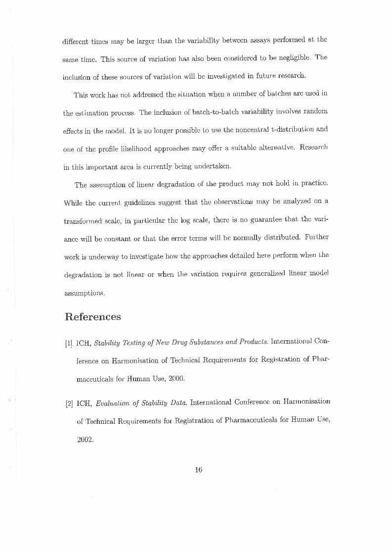
different times may be larger than the variability between assays performed at the
same time. This source of variation has also been considered to be negligible. The
inclusion of these sources of variation will be investigated in future research.
This work has not addressed the situation when a number of batches are used in
the estimation process. The inclusion of batch-to-batch variability involves random
effects in the model. It is no longer possible to use the noncentral t-distribution and
one of the profile likelihood approaches may offer a suitable alternative. Research
in this important area is currently being undertaken.
The assumption of linear degradation of the product may not hold in practice.
White the current guidelines suggest that the observations may be analyzed on a
transformed scale, in particular the log scale, there is no guarantee that the vari-
ance will be constant or that the error terms will be normally distributed. Further
work is underway to investigate how the approaches detailed here perform when the
degradation is not linear or when the variation requires generalized linear model
assumptions.
References
[1] ICH, Stabitity Testi,ng of New Drug Substances and Prodtt'cts.International Con-
ference on Harmonisation of Technical Requirements for Registration of Phar-
maceuticals for Human Use, 2000.
[2] ICH, Eualuati,on of Stability Data.International Conference on Harmonisation
of Technical Requirements for Registration of Pharmaceuticals for Human Use,
2002.
16
[B] Chow SC, Shao J, Estimating drug shelf-life in NDA stability studies. ASA Pro-
ceedings of the Biopharmaceutical Sect'ion, The Americal Statistical Association,
pp. 190-195.
[4] Shao J, Chow SC, Statistical inference in stability analysis. Biometrics 1'994;
50:753-763.
[5] Carstensen JT, Nelson E, Terminology regarding labeled and contained amounts
in dosage forms. Journal of Pharmaceutical sc'iences 1976; 65(2):311-312.
[6] Easterling RG, Discrimination intervals for percentiles in regression. Joumal of
th e Ameri can Statistica'l A s s o ci' ati'on 1969 ; 64 : 1 03 1-1 04 1'
17] Barndorfi-Nielsen OE, On a formula for the distribution of the maximum likeli-
hood estim ator. Biometrika 1983 ; 70 (2) : 343-365.
[8] Cox DR, Reid N, Parameter orthogonality and approximate conditional infer-
ence (with discussion) . Journal of the Royal Statistical Soci'ety - Seri'es B 1987;
a9(1):1-39.
[g] Kiermeier A, A new approach to estimating shelf-llf.e. Tech. rep.,BiometricsSA,
The University of Adelaide/SARDI, 2002'
77
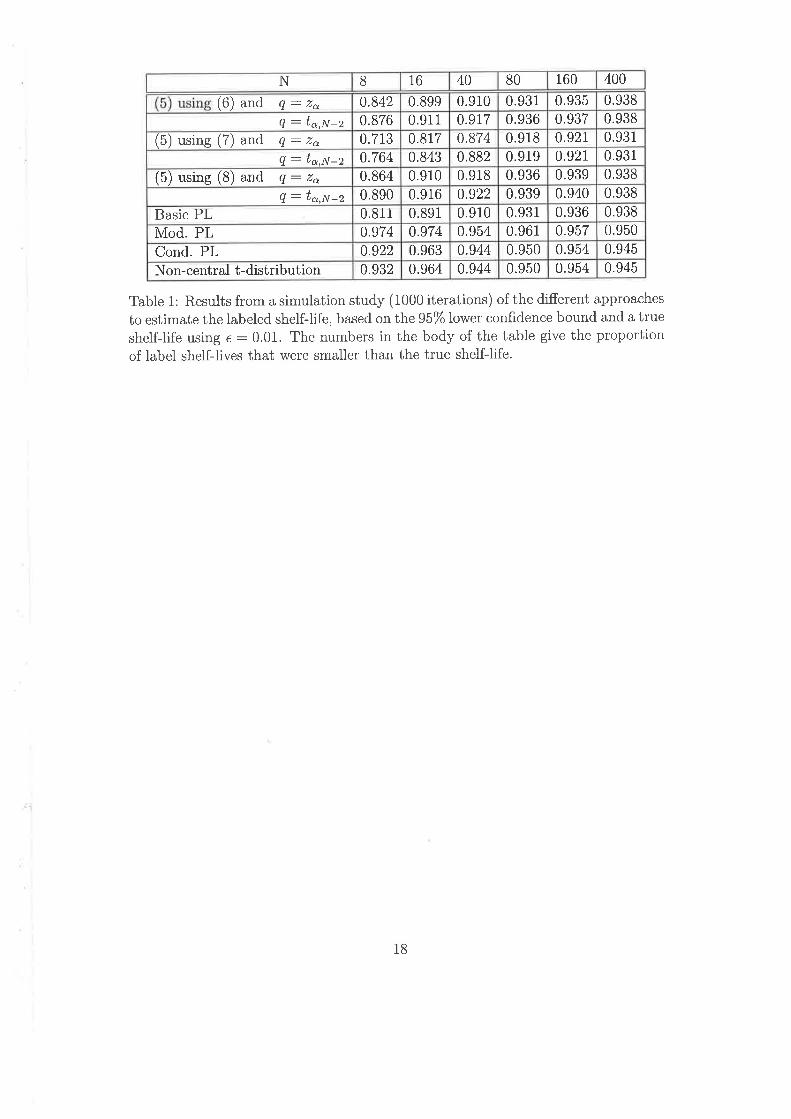
0.9450.9540.9500.9440.9640.932Non-central t-distribution0.9450.9540.9500.9440.9630.922Cond. PL0.9500.9570.9610.9540.9740.974Mod. PL0.9380.9360.9310.9100.8910.811Basic PL
0.9380.9400.9390.9220.9160.890Q: ta,N-z0.9380.9390.9360.9180.9100.864(5) using (8) and 8: za
0.9310.9270.9190.8820.8430.764Q: ta,N-z0.9310.9270.9180.8740.8170.713(5) using (7) and Q: zo
0.9380.9370.9360.9r70.9110.876Q: ta,N-z0.9380.9350.9310.9100.8990.842(6) and e: zo
160 400BO408 16N
Table 1: Results from a simulation study (1000 iterations) of the different approaches
to estimate the labeled shelf-life, based on the 95% Iower confrdence bound and a true
shelf-life using e : 0.01. The numbers in the body of the table give the proportion
of label shelf-lives that were smaller than the true shelf-life.
18
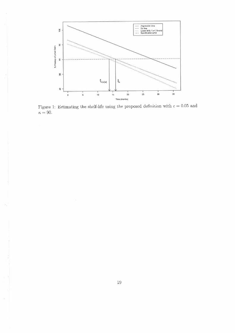
'õ
Ts
ð86ÀàR
0 10 15 20
.fimo (months)
25 30
Figure 1: Estimating the shelf-life using the proposed definition with e : 0.05 and
rc:90.
- R€gresion LlnE
--- 5%lin6Low€r 95% conl Bound
- - Spec¡f¡cation Llm¡t
f€Îe,L(q)
19
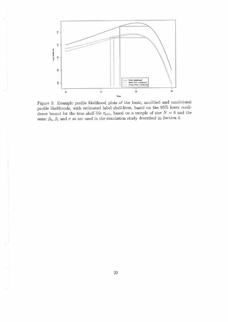
I
I
!Ë
t=o8iJ
I
rm6 20 25
Figure 2: Example profile likelihood plots of the basic, modified and conditionalprofile likelihoods, with estimated label shelf-lives, based on the 95% lower confi'-
dence bound for the true shelf-life r¡.61, based on a sample of size .l : 8 and the
same B6, py and d as are used in the simulation study described in Section 4'
- - - ì¡od Prof. Llkol¡h@d- - Cond Prol Llkelihæd
',1
20