Shasta: Interactive Reporting At Scale

Gokul Nath Babu Manoharanα, Stephan Ellnerα, Karl Schnaitterα, Sridatta Cheguα,Alejandro Estrella-Balderramaα, Stephan Gudmundsonα, Apurv Guptaα, Ben Handyα,Bart Samwelα, Chad Whipkeyα, Larysa Aharkavaα, Himani Apteα, Nitin Gangaharα,

Jun Xuα, Shivakumar Venkataramanα, Divyakant Agrawalα, Jeffrey D. Ullmanβ∗

αGoogle, Inc. βStanford University

ABSTRACTWe describe Shasta, a middleware system built at Google to supportinteractive reporting in complex user-facing applications related toGoogle’s Internet advertising business. Shasta targets applicationswith challenging requirements: First, user query latencies mustbe low. Second, underlying transactional data stores have com-plex “read-unfriendly” schemas, placing significant transformationlogic between stored data and the read-only views that Shasta ex-poses to its clients. This transformation logic must be expressedin a way that scales to large and agile engineering teams. Finally,Shasta targets applications with strong data freshness requirements,making it challenging to precompute query results using commontechniques such as ETL pipelines or materialized views. Instead,online queries must go all the way from primary storage to user-facing views, resulting in complex queries joining 50 or more ta-bles.

Designed as a layer on top of Google’s F1 RDBMS and Mesadata warehouse, Shasta combines language and system techniquesto meet these requirements. To help with expressing complex viewspecifications, we developed a query language called RVL, withsupport for modularized view templates that can be dynamicallycompiled into SQL. To execute these SQL queries with low latencyat scale, we leveraged and extended F1’s distributed query enginewith facilities such as safe execution of C++ and Java UDFs. Toreduce latency and increase read parallelism, we extended F1 stor-age with a distributed read-only in-memory cache. The system wedescribe is in production at Google, powering critical applicationsused by advertisers and internal sales teams. Shasta has signifi-cantly improved system scalability and software engineering effi-ciency compared to the middleware solutions it replaced.

1. INTRODUCTIONMany business applications at Google aim to provide interac-

tive data-rich UIs, allowing users such as advertisers, publishersand video content creators to manage and analyze their data. Itis not uncommon for such applications to combine interactive re-porting (OLAP) and update (OLTP) functionality in the same UI.∗Work performed while at Google, Inc.

Permission to make digital or hard copies of part or all of this work for personal orclassroom use is granted without fee provided that copies are not made or distributedfor profit or commercial advantage and that copies bear this notice and the full citationon the first page. Copyrights for third-party components of this work must be honored.

SIGMOD/PODS’16 June 26 - July 01, 2016, San Francisco, CA, USAc© 2016 Copyright held by the owner/author(s).

ACM ISBN 978-1-4503-3531-7/16/06.

DOI: http://dx.doi.org/10.1145/2882903.2904444

For a representative example, consider AdWords, Google’s searchadvertising product: In a Web UI, advertisers configure their cam-paigns. Campaign configurations are stored in the F1 database [13]in hundreds of normalized tables backed by Spanner storage [5].Google serves ads based on these configurations, and log aggrega-tion systems [1] use ad server logs to continuously update hundredsof metrics tables stored in Mesa [8], tracking the performance of therunning ad campaigns in near real-time. Deeply integrating OLTPand OLAP functionality, the AdWords Web UI allows advertisers toview interactive reports with campaign performance metrics and tomake changes to campaign configurations. Corresponding SOAPdeveloper APIs allow advertisers to interact with their campaignand reporting data programmatically.

A challenge in scaling such applications in practice are vast data-base schemas with hundreds of tables, placing significant transfor-mation logic between stored data and user-facing concepts. This“concept gap” tends to be particularly wide for OLAP functional-ity, posing non-trivial questions for application designers:• How to encapsulate complex data transformations? Without

proper abstractions, business logic tends to leak into inappropri-ate parts of the system or get duplicated, creating problems forcode ownership, readability, consistency, and release velocity.

• How to express the transformations? Even if business logicis encapsulated well, the right paradigm to express it is non-obvious. Procedural languages such as Java or C++ are pow-erful, but can be cumbersome for expressing complex queryoperations on top of vast database schemas, e.g., joins of 50 ta-bles. SQL on the other hand naturally captures relational opera-tions, but doesn’t scale gracefully to code artifacts of thousandsof lines of code. Furthermore, applications that allow users tointeractively change data visualization parameters such as col-umn selection, segmentations, and filters require that develop-ers express queries with a large degree of dynamic variation inquery operations such as joins, aggregations, and filters.

• How to compute the transformations? Deciding during whichphase of data processing to compute the transformations posesawkward tradeoffs. A common data warehousing approach isto rely on precomputation, maintaining a “read-friendly” denor-malized copy of transactional data optimized for OLAP work-loads [4]. If the denormalized copy is stale with respect to data-base updates, it tends to not satisfy applications with a high barfor fresh and consistent data, and the necessary offline pipelinestend to make systems more stateful and operationally complex.Transactionally updated materialized views on the other handincrease the cost of writes. Finally, computing most transfor-mations as part of online queries makes achieving interactive(sub-second) latencies challenging, especially if queries read

1393

from multiple data stores with different performance character-istics.

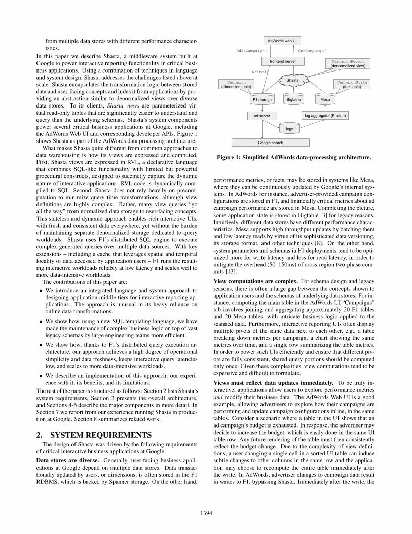
In this paper we describe Shasta, a middleware system built atGoogle to power interactive reporting functionality in critical busi-ness applications. Using a combination of techniques in languageand system design, Shasta addresses the challenges listed above atscale. Shasta encapsulates the transformation logic between storeddata and user-facing concepts and hides it from applications by pro-viding an abstraction similar to denormalized views over diversedata stores. To its clients, Shasta views are parameterized vir-tual read-only tables that are significantly easier to understand andquery than the underlying schemas. Shasta’s system componentspower several critical business applications at Google, includingthe AdWords Web UI and corresponding developer APIs. Figure 1shows Shasta as part of the AdWords data processing architecture.

What makes Shasta quite different from common approaches todata warehousing is how its views are expressed and computed.First, Shasta views are expressed in RVL, a declarative languagethat combines SQL-like functionality with limited but powerfulprocedural constructs, designed to succinctly capture the dynamicnature of interactive applications. RVL code is dynamically com-piled to SQL. Second, Shasta does not rely heavily on precom-putation to minimize query time transformations, although viewdefinitions are highly complex. Rather, many view queries “goall the way” from normalized data storage to user-facing concepts.This stateless and dynamic approach enables rich interactive UIs,with fresh and consistent data everywhere, yet without the burdenof maintaining separate denormalized storage dedicated to queryworkloads. Shasta uses F1’s distributed SQL engine to executecomplex generated queries over multiple data sources. With keyextensions – including a cache that leverages spatial and temporallocality of data accessed by application users – F1 runs the result-ing interactive workloads reliably at low latency and scales well tomore data-intensive workloads.

The contributions of this paper are:• We introduce an integrated language and system approach to

designing application middle tiers for interactive reporting ap-plications. The approach is unusual in its heavy reliance ononline data transformations.

• We show how, using a new SQL templating language, we havemade the maintenance of complex business logic on top of vastlegacy schemas by large engineering teams more efficient.

• We show how, thanks to F1’s distributed query execution ar-chitecture, our approach achieves a high degree of operationalsimplicity and data freshness, keeps interactive query latencieslow, and scales to more data-intensive workloads.

• We describe an implementation of this approach, our experi-ence with it, its benefits, and its limitations.

The rest of the paper is structured as follows: Section 2 lists Shasta’ssystem requirements, Section 3 presents the overall architecture,and Sections 4-6 describe the major components in more detail. InSection 7 we report from our experience running Shasta in produc-tion at Google. Section 8 summarizes related work.

2. SYSTEM REQUIREMENTSThe design of Shasta was driven by the following requirements

of critical interactive business applications at Google:

Data stores are diverse. Generally, user-facing business appli-cations at Google depend on multiple data stores. Data transac-tionally updated by users, or dimensions, is often stored in the F1RDBMS, which is backed by Spanner storage. On the other hand,

MesaF1 storage

logs

Google search

AdWords web UI

EditCampaign() GetCampaign()

write()

Bigtable

Campaign (dimension table)

CampaignStats (fact table)

CampaignReport (denormalized view)

frontend server

ad server log aggregator (Photon)

Shasta

Figure 1: Simplified AdWords data-processing architecture.

performance metrics, or facts, may be stored in systems like Mesa,where they can be continuously updated by Google’s internal sys-tems. In AdWords for instance, advertiser-provided campaign con-figurations are stored in F1, and financially critical metrics about adcampaign performance are stored in Mesa. Completing the picture,some application state is stored in Bigtable [3] for legacy reasons.Intuitively, different data stores have different performance charac-teristics. Mesa supports high throughput updates by batching themand low latency reads by virtue of its sophisticated data versioning,its storage format, and other techniques [8]. On the other hand,system parameters and schemas in F1 deployments tend to be opti-mized more for write latency and less for read latency, in order tomitigate the overhead (50–150ms) of cross-region two-phase com-mits [13].

View computations are complex. For schema design and legacyreasons, there is often a large gap between the concepts shown toapplication users and the schemas of underlying data stores. For in-stance, computing the main table in the AdWords UI “Campaigns”tab involves joining and aggregating approximately 20 F1 tablesand 20 Mesa tables, with intricate business logic applied to thescanned data. Furthermore, interactive reporting UIs often displaymultiple pivots of the same data next to each other, e.g., a tablebreaking down metrics per campaign, a chart showing the samemetrics over time, and a single row summarizing the table metrics.In order to power such UIs efficiently and ensure that different piv-ots are fully consistent, shared query portions should be computedonly once. Given these complexities, view computations tend to beexpensive and difficult to formulate.

Views must reflect data updates immediately. To be truly in-teractive, applications allow users to explore performance metricsand modify their business data. The AdWords Web UI is a goodexample, allowing advertisers to explore how their campaigns areperforming and update campaign configurations inline, in the sametables. Consider a scenario where a table in the UI shows that anad campaign’s budget is exhausted. In response, the advertiser maydecide to increase the budget, which is easily done in the same UItable row. Any future rendering of the table must then consistentlyreflect the budget change. Due to the complexity of view defini-tions, a user changing a single cell in a sorted UI table can inducesubtle changes to other columns in the same row and the applica-tion may choose to recompute the entire table immediately afterthe write. In AdWords, advertiser changes to campaign data resultin writes to F1, bypassing Shasta. Immediately after the write, the

1394

frontend server may request table data for the given Shasta viewand expect subsequent queries to return fresh and consistent data,taking into account the most recent update by the user.

View queries from interactive UIs must be fast. Shasta queriesare on the critical path to rendering pages in user-facing applica-tions with sub-second latency targets. Importantly, interfaces andAPIs in such applications are often scoped to an individual user’sbusiness data, so that typical Shasta queries process only a mod-est subset of data in underlying data stores. Still, individual fullyoptimized queries can scan gigabytes of raw data from 50 or morephysical tables, and the transformations required for a query can becomputationally demanding. Fortunately, interactive applicationstend to be used in user sessions, allowing Shasta to leverage tem-poral and spatial locality of accessed data.

View definitions are parameterized. To its clients, Shasta viewsare parameterized virtual tables, which provide access to denormal-ized data while hiding complex storage schemas with hundreds oftables. Issuing a Shasta query is straightforward: The client speci-fies a view name, a list of column names, a simple specification forhow to filter and sort resulting rows, and more ad-hoc parametersthat customize the view semantics. To answer a given Shasta query,Shasta then needs to compute the view in the context of the givenparameters. In practice, parameter values can have a major effecton the semantics of a view. For instance, depending on whether theuser is part of a feature whitelist, a Shasta view may require data tobe read from different tables and joined in a different structure.

View implementation must be manageable. In practice, hun-dreds of software engineers across different teams need to modifyshared view definitions and schemas. Resulting changes need tobe released to production multiple times per week, without down-time. In order to achieve these goals, Shasta needs a view definitionformat that helps developers easily reason about and modify views,and this format needs to scale to complex and highly parameterizedview definitions. Ideally, view definitions should be mostly declar-ative, but views must be allowed to invoke some application codewritten in a procedural language such as C++ or Java.

3. SYSTEM ARCHITECTUREIn principle, it would be reasonable to express Shasta view trans-

formations using SQL and leverage F1’s distributed query enginefor scalable query execution, since the transformations required byShasta views are a natural fit for SQL. However, it is challengingin practice to define Shasta views in terms of SQL and meet thelatency requirements of interactive applications, given the complexnature of queries. Shasta’s system architecture overcomes thesetwo challenges, thus allowing query execution to be handled by F1.

In order to push all computation to F1, Shasta needs to trans-late each client query into a single SQL query. This is difficultdue to the complexity of data transformations, paired with a widevariety of queries corresponding to different view parameter val-ues. The Shasta architecture simplifies the task of SQL generation:View definitions are expressed in a new language called RVL andare translated to SQL using a just-in-time compiler. The syntax ofRVL is SQL-like, but extended with higher-level constructs whichmake it easier to define Shasta views concisely while accountingfor dynamic view parameters. RVL supports user-defined functions(UDFs), allowing Shasta view definitions to invoke procedural ap-plication code.

The following extensions to the F1 query engine were made tomeet the needs of Shasta:

F1 Query Engine

Frontend Server

F1 Coordinator

F1 Slave

F1 storage BigtableMesa

RVL codeRVL codeRVL CodeView Gateway RVL Compiler

read (Shasta query)

SQL

write

TableCache UDF Server

Figure 2: Shasta architecture.

• We improved support for UDFs in F1. Specifically, we added acomponent called UDF server to F1, which supports safe eval-uation of compiled C++ and Java UDFs with high throughput.

• In order to meet the latency constraints of Shasta, we addedan in-memory read-only cache between F1 storage and queryengine, called TableCache. Shasta uses TableCache to accessconsistent snapshots of F1 data significantly faster than readingfrom F1 storage directly. The cache is kept up-to-date usinga light-weight protocol based on F1’s Change History feature.For Shasta applications, maintaining similar caches for otherdata sources such as Mesa and Bigtable has proven either lesscritical or too expensive in practice.

Figure 2 shows how the components of Shasta fit together to an-swer queries. A query issued by the application’s frontend serverspecifies a view name, columns to query, and view parameters suchas application user ID or feature ID. In addition, the client oftenspecifies a timestamp, which tells Shasta to use F1 data which isconsistent with the snapshot at that timestamp. Exposing the list ofavailable view schemas to application developers is typically donevia shared code repositories. The view gateway receives the Shastaquery and invokes the RVL compiler with view parameter bindingsto generate a potentially large SQL string. The F1 query engineexecutes the generated SQL, using UDF servers to evaluate anyUDFs in the query. TableCache accelerates access to F1 storageduring query execution, while the query engine reads directly fromdata sources other than F1 such as Mesa and Bigtable. F1 supportsaccess to such “external” data sources using a plugin API [13], al-lowing for tight integration with the query engine. F1 pushes filtersand projections to external data sources where possible, performingother computations itself. Optimizations that would delegate morecomplex query operations to external data sources [9] are left asfuture work.

It is worth noting that Shasta does not rely on precomputationand materialization of intermediate view query results. Althoughprecomputation may improve the latency of Shasta queries, it tendsto be a poor fit for Shasta applications, especially when dealingwith financial user data: Keeping materialized results synchronizedwith user-issued changes to underlying data stores makes writesmore expensive, which is often not an option. It would also beimpractical to use stale materializations while satisfying freshnessrequirements, due to the complexity of Shasta views. These draw-backs can be avoided by evaluating queries on raw data.

The following sections provide more details on RVL (Section 4),Shasta’s use of the F1 query engine and UDF servers (Section 5),and TableCache (Section 6).

1395

Request Handler

RVL Compiler

Shasta Query

Generated SQL Query

Query Result

Template Parameter Bindings

RVL Code

Table Metadata

View Gateway

F1 SQL Execution

Figure 3: Using the RVL compiler in Shasta.

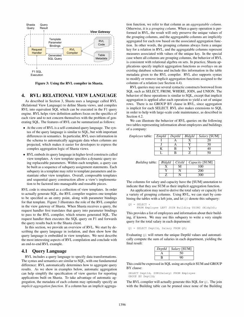
4. RVL: RELATIONAL VIEW LANGUAGEAs described in Section 3, Shasta uses a language called RVL

(Relational View Language) to define Shasta views, and compilesRVL into equivalent SQL which can be executed in the F1 queryengine. RVL helps view definition authors focus on the specifics ofeach view and to not concern themselves with the problem of gen-erating SQL. The features of RVL can be summarized as follows:

• At the core of RVL is a self-contained query language. The syn-tax of the query language is similar to SQL, but with importantdifferences in semantics. In particular, RVL uses information inthe schema to automatically aggregate data when columns areprojected, which makes it easier for developers to express thecomplex aggregation logic of Shasta views.

• RVL embeds its query language in higher-level constructs calledview templates. A view template specifies a dynamic query us-ing replaceable parameters. Within each template, a query canbe built as a sequence of subquery assignment statements. Eachsubquery in a template may refer to template parameters and in-stantiate other view templates. Overall, composable templatesand sequential query construction allow a view’s implementa-tion to be factored into manageable and reusable pieces.

RVL code is structured as a collection of view templates. In orderto actually generate SQL, the RVL compiler requires one templateto be specified as an entry point, along with parameter bindingsfor that template. Figure 3 illustrates the role of the RVL compilerin the view gateway of Shasta. When Shasta receives a query, therequest handler first translates that query into parameter bindingsto pass to the RVL compiler, which returns generated SQL. Therequest handler then executes the SQL query on F1 and forwardsthe query results back to the Shasta client.

In this section, we provide an overview of RVL. We start by de-scribing the query language in isolation, and then show how thequery language is embedded in view templates. We next describethe most interesting aspects of RVL compilation and conclude withan end-to-end RVL example.

4.1 Query LanguageRVL includes a query language to specify data transformations.

The syntax and semantics are similar to SQL, with one fundamentaldifference: RVL automatically determines how to aggregate queryresults. As we show in examples below, automatic aggregationcan help simplify the specification of view queries for reportingapplications built on Shasta. To take advantage of automatic ag-gregation, the metadata of each column may optionally specify animplicit aggregation function. If a column has an implicit aggrega-

tion function, we refer to that column as an aggregatable column.Otherwise, it is a grouping column. When a query operation is per-formed in RVL, the result will only preserve the unique values ofthe grouping columns, and the aggregatable columns are implicitlyaggregated for each row based on the associated aggregation func-tion. In other words, the grouping columns always form a uniquekey for a relation in RVL, and the aggregatable columns representmeasures associated with values of the unique key. In the specialcase where all columns are grouping columns, the behavior of RVLis consistent with relational algebra on sets. In practice, Shasta ap-plications specify implicit aggregation functions as overlays on anexisting database schema and include this information in the tablemetadata given to the RVL compiler. RVL also supports syntaxto modify or remove implicit aggregation functions assigned to thecolumns of a relation (see Section 4.4).

RVL queries may use several syntactic constructs borrowed fromSQL such as SELECT, FROM, WHERE, JOIN, and UNION. Thebehavior of these operations is similar to SQL, except that implicitaggregation is applied after each operation to yield a set of uniquerows. There is no GROUP BY clause in RVL, since aggregationis implicit for each SELECT. RVL also makes extensions to SQLin order to help with large-scale code maintenance, as described inSection 4.2.

We can illustrate the behavior of RVL queries on the followingtwo tables representing information about employees and buildingsof a company:

Employee table: EmpId DeptId BldgId Salary [SUM]I A X 20J A Y 30K B Y 40L B Z 50

Building table: BldgId CityId Capacity [SUM]X M 100Y N 200Z N 300

The columns for salary and capacity have the [SUM] annotation toindicate that they use SUM as their implicit aggregation function.

An application may need to derive the total salary or capacity fora variety of grouping columns. Using RVL, we can start by com-bining the tables with a left join, and let Q0 denote this subquery:

Q0 = SELECT *FROM Employee LEFT JOIN Building USING (BldgId);

This provides a list of employees and information about their build-ing, if known. We may use this subquery to write a very simplequery for the total salary in each department:

Q1 = SELECT DeptId, Salary FROM Q0;

Evaluating Q1 will return the unique DeptId values and automati-cally compute the sum of salaries in each department, yielding thefinal result:

DeptId Salary [SUM]A 50B 90

This could be expressed in SQL using an explicit SUM and GROUPBY clause:SELECT DeptId, SUM(Salary) FROM EmployeeGROUP BY DeptId;

The RVL compiler will actually generate this SQL for Q1. The joinwith the Building table can be pruned since none of the Building

1396

columns are required. Join pruning is a key feature of RVL, whichwe discuss in Section 4.3.

Implicit aggregation becomes more interesting when data is re-quested from both tables. For example:

Q2 = SELECT CityId, Salary, Capacity FROM Q0;

This will return the unique CityId values and automatically com-pute the total salaries of employees in each city, along with thecapacity of the buildings in that city:

CityId Salary [SUM] Capacity [SUM]M 20 100N 120 500

The RVL compiler generates the following SQL representation ofQ2 which adds two GROUP BY steps:

SELECT CityId, SUM(Salary) AS Salary,SUM(Capacity) AS Capacity

FROM(SELECT BldgId, SUM(Salary) AS SalaryFROM Employee GROUP BY BldgId)

LEFT JOIN Building USING (BldgId))GROUP BY CityId;

Observe that the inner subquery removes EmpId and DeptId, inorder to aggregate the remaining columns of the Employee tablebefore the join. The inner aggregation ensures that the capacity iscomputed correctly. If we naively removed all unwanted columnsafter the join and performed the aggregation in a single step, the ca-pacity values would be multiplied by the number of employees ineach building. Our desired result should only count the capacity ofeach building once. We will revisit this example and the RVL com-piler’s strategy for arranging GROUP BY clauses in Section 4.3.

The value of RVL can be seen by comparing Q1 and Q2 to thecorresponding SQL representations. In RVL, we can define a sin-gle subquery Q0 such that Q1 and Q2 can be expressed as simpleprojections over Q0. In contrast, the SQL representations of Q1 andQ2 have drastically different structure. RVL also makes it easy toderive meaningful aggregate values from Q0 for many other com-binations of grouping columns. A direct SQL representation of allpossible projections over the join would need to account for all thepotential arrangements of GROUP BY clauses and invocations ofaggregation functions. In practice, real Shasta queries can be morecomplex, requiring dozens of tables to be joined. It becomes chal-lenging for developers to formulate the correct aggregation seman-tics using SQL directly whereas formulating queries using RVLmakes it much more simple and intuitive.

4.2 View TemplatesAs described above, the RVL query language provides implicit

aggregation to help developers express aggregation semantics whenthe set of requested columns is not fixed. However, implicit aggre-gation does not solve all the challenges of implementing Shastaviews. In particular:• The parameters of a Shasta view may have a large impact on

the RVL query. For instance, the view parameters may changethe tables used in joins or the placement of filters in the query.RVL needs to be more dynamic in order to capture this widerange of possible query structures.

• An RVL query could grow quite large with many column trans-formations and deeply nested joins. A typical Shasta view wouldrequire 100s of lines of code, and expressing that as a singlelarge query can be difficult to read and maintain.

RVL view templates solve these problems. View templates allowlarge queries to be constructed dynamically from smaller pieces

which can be composed and reused by multiple Shasta views. Aview template takes input parameters which are used to representthe dynamic aspects of a query (e.g., list of requested columns),and returns a corresponding RVL query using the parameter values.In other words, for any fixed choice of parameter values, a viewtemplate is shorthand for an RVL query (similar to the traditionalnotion of a view).

A view template may be referenced in the FROM clause of RVLqueries by passing values for its input parameters, and the referencewill be replaced with the query generated by the view template. Thefollowing values may be bound to view template parameters:• RVL text: A string containing valid RVL syntax can be bound

to a view template parameter, and that parameter can be refer-enced in places where it would be valid to inject the RVL syntaxstring. For example, a template parameter bound to the string"X,Y" could be referenced in a SELECT clause, and the tem-plate parameter reference will behave exactly as if "X,Y" werewritten directly in the query.

• Nested dictionary: A template parameter can be bound to adictionary of name-value pairs, where the values can either beanother dictionary, or RVL text. Intuitively, a nested dictionaryis a collection of RVL text parameters with hierarchical names.

• Subquery: A template parameter can be bound to an RVL sub-query, and referenced anywhere a table can be referenced. Asubquery value differs from RVL text values, in the sense thatsubquery values are substituted in a purely logical manner whichis independent of the syntax used to create the subquery. In con-trast, an RVL text value is purely a text injection, which allowsany variables in the RVL text to be interpreted based on thecontext where the parameter is referenced.

RVL text values allow RVL parameters to be more flexible than tra-ditional SQL runtime parameters, since RVL allows parameters torepresent large substructures of queries. However, RVL text valuesdo not allow for arbitrary code injection. In order to make viewtemplates less error-prone, an RVL text value is only allowed tocontain a few specific syntactic forms, such as scalar expressions,expression lists, and base table names. There are also strict rulescontrolling the locations where each syntactic form can be substi-tuted.

We use the following example to illustrate the basic templatesyntax and semantics:

view FilterUnion<input_table, params> {T1 = SELECT $params.column_name FROM $input_table;T2 = SELECT $params.column_name FROM Employee;T = T1 UNION T2;return SELECT * FROM T

WHERE $params.column_name >= $params.min_value;}

The view template contains three assignment statements which givealiases to subqueries, and the fourth statement returns the finalquery. There are two template parameters:• input_table can be bound to a table name or subquery. It is

referenced in the first FROM clause as $input_table.

• params must be bound to a nested dictionary. In this example,$params.column_name should be the name of a column in$input_table, and $params.min_value is a lower boundthat we want to apply to that column.

The behavior of the view template is intuitive: The first two state-ments fetch a dynamically chosen column from the $input_tableparameter as well as the Employee table, the third statement com-bines the two sets of values, and the final statement applies a lowerbound to the values before returning them.

1397

A view template can be designated as an entry point in the RVLcode, in which case it is called a main view template. RVL providesan API to invoke a main view template, with a nested dictionary asa parameter. The main view template can use one or more outputstatements to specify the desired result. For example, using theprevious FilterUnion view template:

main OutputValues<params> {b = SELECT * FROM Building;all_values = SELECT * from FilterUnion<@b, $params>;output all_values AS result;

}

The output statement specifies a table to produce as the final resultwhen the main view template is invoked, as well as an alias for thattable. If there are multiple output statements, the aliases must beunique so that the Shasta view gateway can distinguish the results.Multiple output statements can reference the same RVL subqueryby name which is useful when applications need to display multi-ple pivots of the same shared view computation. To achieve con-sistency between different data pivots within a view query, RVLguarantees that each named subquery is only executed once.

In Section 4.4 we present a larger RVL example which uses ad-ditional syntax features. Most interestingly, RVL view templatesmay use control structures written as if/else blocks to dynamicallychoose between two or more subqueries.

4.3 RVL Compiler and Query OptimizationThe RVL compiler generates SQL which will produce the out-

put tables specified by a main view template, given the requiredparameter bindings. Shasta executes the generated SQL using theF1 query engine, taking advantage of F1’s query optimizations anddistributed execution. In order to perform SQL generation, the RVLcompiler first resolves references to view templates and named sub-queries, producing an algebraic representation of an RVL queryplan that includes all outputs of the invoked main view template.The RVL compiler performs some transformations to optimize andsimplify the query plan before translating it to SQL. In this section,we describe some details of RVL query optimization and explainwhy it is important.

The RVL compiler optimizes query plans using a rule-based en-gine. Each rule uses a different strategy to simplify the plan basedon algebraic structure, without estimating cost. In practice, rule-based optimization is sufficient because the only goal is to simplifythe generated SQL, rather than determine all details of query execu-tion. We avoid using cost-based optimization because a cost modelwould tie the RVL compiler to a specific SQL engine and make itless generic.

The intuitive reason to optimize an RVL query plan before gen-erating SQL (as opposed to relying on F1 for all optimizations) isto take advantage of RVL’s implicit aggregation semantics. Severaloptimization rules are implemented in the RVL compiler relying onproperties of implicit aggregation to ensure correctness. The RVLcompiler also implements optimization rules which do not dependdirectly on implicit aggregation, because they interact with otherrules that do depend on implicit aggregation and make them moreeffective. We describe a few of the more interesting rules below.

Column Pruning: Recall the Employee/Building example earlierin this section. Our SQL representation of Q2 performed a projec-tion and aggregation before the join, which differs from the orderof operations in the RVL for Q2. The join and aggregation stepsare reordered by an RVL optimization rule called column pruning.Without column pruning, the equivalent SQL representation of Q2would be:

SELECT CityId, SUM(Salary) AS Salary,SUM(Capacity) AS Capacity

FROM(SELECT BldgId, CityId,

SUM(Salary) AS Salary, CapacityFROM Employee LEFT JOIN Building USING (BldgId)GROUP BY BldgId, CityId, Capacity)

GROUP BY CityId;

Observe that this SQL representation performs two stages of aggre-gation after the join, in order to compute correct aggregate valuesfor both salary and capacity. A sufficiently advanced SQL opti-mizer may be able to optimize this query by pushing the inner ag-gregation below the join, but this is a difficult optimization to gen-eralize in the context of SQL [16]. For larger RVL queries, the SQLrepresentation may become much more complicated when comput-ing aggregate values after joining. In the worst case, an implicitaggregation may require aggregatable columns to be computed ina temporary table and joined back into the original query. Thatpattern in particular is extremely difficult for a SQL engine to opti-mize, so column pruning is needed in order to simplify the task ofthe F1 query optimizer. Moreover, the logic for pruning columnsin the RVL compiler is straightforward due to implicit aggregationsemantics. For all these reasons, the RVL compiler aggressivelyprunes unneeded columns and performs aggregations before joinswhenever possible.

Filter Pushdown: In a SQL database, filter pushdown could beconsidered one of the most basic optimizations, where the goal isto filter data as early as possible in the query plan. At first glance,it might seem unnecessary for RVL to push down filters, since theF1 query optimizer is fully capable of performing this optimiza-tion. However, filter pushdown can improve the effectiveness ofthe column pruning optimization. For example, if there is a filteron a column which is not part of the final result, the filter will pre-vent column pruning from removing the column before the filter isapplied. It is crucial for the filter to be pushed down as early aspossible in the query plan, so that the column can be pruned earlyas well.

Left Join Pruning: In RVL, if a left join does not require any of thecolumns from its right input, the right input can be removed fromthe query plan. In a general SQL database, this optimization is lessobvious and less likely to apply, since a left join may duplicate rowsin the left input. Consider the following example of a SQL left join,using the example Employee and Building tables:

SELECT EmpId, SUM(Salary)FROM Employee LEFT JOIN Building USING (BldgId);

If it is known that each Employee row will join with at most onerow in the Building table, the join can be pruned, resulting in:

SELECT EmpId, SUM(Salary) FROM Employee;

A SQL optimizer might be able to perform this optimization if itknows that BldgId is a unique key of the Building table. The op-timization would become more difficult to do if the Building tablewere replaced with a complex subquery. On the other hand, theleft join in RVL is trivial to prune, since the inputs of the join arealways guaranteed to be sets, and the column pruning optimizationwill prune all Building columns except BldgId.

The join pruning optimization makes RVL programming moreconvenient. A user can add many left joins to their view templatesto fetch columns which might not be required, and they can be con-fident that the RVL compiler will know which joins can be skipped.

4.4 Example View TemplateFigure 4 shows example schemas for F1 and Mesa tables, using

advertising concepts from the AdWords application. The example

1398

Customer(root table) BudgetSuggestionV1 BudgetSuggestionV2CustomerId CustomerInfo

20 { name: "flowers" }CustomerId BudgetId SuggestionInfo

20 200 { suggested_amount: 120 }CustomerId BudgetId SuggestionInfo

20 200 { suggested_amount: 118 }

Campaign BudgetCustomerId CampaignId CampaignInfo

20 100 { name: "Rose" status: "ENABLED" budget_id: 200 }20 101 { name: "Tulip" status: "ENABLED" budget_id: 200 }20 102 { name: "Daisy" status: "ENABLED" budget_id: 201 }

CustomerId BudgetId BudgetInfo20 200 { amount: 100 }20 201 { amount: 50 }

CampaignStats CampaignConversionStatsCustomerId CampaignId Device Impressions Clicks Cost

20 100 ’Desktop’ 20 5 320 100 ’Tablet’ 10 3 120 101 ’Mobile’ 30 4 220 102 ’Desktop’ 40 10 5

CustomerId CampaignId Device ConversionType Conversions20 100 ’Desktop’ ’Purchase’ 220 100 ’Desktop’ ’Wishlist’ 120 101 ’Mobile’ ’Wishlist’ 2

Figure 4: Example storage schema. Bolded column names refer to primary keys.

view CampaignDimensions<params> {campaign = SELECT *,CampaignInfo.name AS Name,CampaignInfo.budget_id AS BudgetIdFROM Campaign;

budgets = SELECT *,BudgetInfo.amount AS BudgetAmountFROM Budget;

budget_suggestion_table =if ($params.use_budget_suggestion_v2) {

BudgetSuggestionV2;} else {

BudgetSuggestionV1;}

budgets_with_suggestion = SELECT *FROM budgets LEFT JOIN budget_suggestion_tableUSING CustomerId, BudgetId;

return SELECT *,ComputeCampaignStatus(CampaignInfo, BudgetInfo,

BudgetSuggestionInfo) AS StatusFROM campaign LEFT JOIN budgets_with_suggestionUSING CustomerId, BudgetId;

}view CampaignFacts<params> {return SELECT *,MakePair(Impressions, Clicks)

AS ClickThroughRate [aggregation = "RateAgg"]FROM CampaignStats FULL JOIN CampaignConversionStats;

}main CampaignReport<params> {campaign_report = SELECT $params.main_table_columnsFROM CampaignDimensions<$params>

LEFT JOIN CampaignFacts<$params>USING CustomerId, CampaignId;

output SELECT *FROM campaign_reportWHERE $params.filtersORDER BY $params.order_by_columnsLIMIT $params.limit as top_k_table;

output SELECT $params.summary_columnsFROM campaign_report as summary;

}

Figure 5: CampaignReport RVL code.

uses F1 dimension tables Customer, Campaign, Budget, Budget-SuggestionV1, and BudgetSuggestionV2, using CustomerId as theroot ID BudgetSuggestionV1 and BudgetSuggestionV2 tables cap-ture a case that often comes up in practice: The application is mi-grating from an older to a newer, higher quality representation ofbudget suggestions. The application may want to use the new sug-gestions for only a small whitelist of advertisers initially, and rampup slowly to all customers. We therefore maintain both versionsduring the transition period. Since different teams maintain the re-spective backend pipelines, separate tables help clarify ownership.

The example also uses Mesa fact tables CampaignStats and Cam-paignConversionStats. Impressions, Clicks, Cost, and Conversionscolumns use SUM for implicit aggregation. CampaignConversion-Stats is a separate table because conversions can be broken downby the additional dimension ConversionType.

Abstracting over the complex storage schema, Shasta exposesa flat denormalized view CampaignReport. The view schema ex-poses the following columns: CustomerId, CampaignId, Name,Status, BudgetAmount, Device, Impressions, ClickThroughRate,Clicks, and Conversions. RVL code for CampaignReport is shownin Figure 5. The following aspects are worth noting:

• The CampaignDimensions view template performs a join of F1tables. The input parameter use_budget_suggestion_v2 in-dicates which version of budget suggestion to use. The Statuscolumn is computed with a user-defined function (UDF).

• The CampaignFacts view template performs a join of Mesa ta-bles. ClickThroughRate is made explicitly aggregatable by auser-defined aggregation function (UDAF) RateAgg. No ex-plicit GROUP BY is specified, as the RVL compiler generatesthe correct GROUP BY clauses based on the request context.

• The main view template CampaignReport joins data from Cam-paignDimensions and CampaignFacts. The two view outputstop_k_table and summary share the campaign_report sub-query, ensuring consistency of the two data pivots.

• params.filters typically contains a filter on CustomerId,but it can also contain filters on aggregatable columns like Im-pressions. The RVL code filters the data after projecting thefinal columns, but the RVL compiler may move filters to beapplied earlier when possible.

Figure 6 illustrates the entire flow of a sample Shasta query with(i) a specific Shasta query issued by a Shasta client against the"CampaignReport" Shasta view, (ii) RVL template parameters gen-erated from the Shasta query by the view gateway, and (iii) theShasta query result. Note the result contains only two campaignsbecause of the "limit: 2" clause in the query, while the summaryrow contains aggregate stats for all campaigns.

5. QUERY EXECUTION ON F1F1’s SQL query engine has been described in [13]. It supports

both centralized and distributed execution of queries. Centralizedexecution can deliver low latencies for simple queries with inputdata volumes that are easily processed on a single F1 server, anddistributed F1 queries are a natural fit for workloads with larger in-

1399

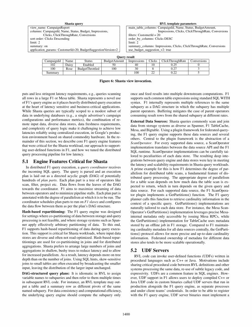
Shasta query RVL template parametersview_name: CampaignReportcolumns: CampaignId, Name, Status, Budget, Impressions,

Clicks, ClickThroughRate, Conversionssort order: Clicks Descendinglimit: 2summary: onapplication_params: CustomerId=20, BudgetSuggestionVersion=2

main_table_columns: CampaignId, Name, Status, BudgetAmount,Impressions, Clicks, ClickThroughRate, Conversions

filters: CustomerId = 20order_by_columns: Clicks DESClimit: 2summary_columns: Impressions, Clicks, ClickThroughRate, Conversionsuse_budget_suggestion_v2: true

Query resultCampaignId Name Status BudgetAmount Impressions Clicks ClickThroughRate Conversions

102 Daisy Enabled 50 40 10 0.25 0100 Rose BudgetThrottled 100 30 8 0.27 3

Summary 100 22 0.22 5

Figure 6: Shasta view invocation.

puts and less stringent latency requirements, e.g., queries scanningall rows in a large F1 or Mesa table. Shasta represents a novel useof F1’s query engine as it places heavily distributed query executionat the heart of latency sensitive and business-critical applications.While Shasta queries are typically scoped to a modest subset ofdata in underlying databases (e.g., a single advertiser’s campaignconfigurations and performance metrics), the combination of re-mote input data, diverse data stores, data freshness requirements,and complexity of query logic make it challenging to achieve lowlatencies reliably using centralized execution, in Google’s produc-tion environment based on shared commodity hardware. In the re-mainder of this section, we describe core F1 query engine featuresthat were critical for the Shasta workload, our approach to support-ing user-defined functions in F1, and how we tuned the distributedquery processing pipeline for low latency.

5.1 Engine Features Critical for ShastaIn distributed F1 query execution, a query coordinator receives

the incoming SQL query. The query is parsed and an executionplan is laid out as a directed acyclic graph (DAG) of potentiallyhundreds of plan parts. Each plan part is a tree of operators likescan, filter, project etc. Data flows from the leaves of the DAGtowards the coordinator. F1 aims to maximize streaming of databetween operators and to minimize pipeline stalls. Each plan part isannotated with the degree of parallelism at which it is to be run. Thecoordinator schedules plan parts to run on F1 slaves and configuresthe data flow between them as per the plan’s DAG structure.Hash-based repartitioning: The F1 query engine was designedfor settings where co-partitioning of data between storage and queryprocessing is not feasible, and where storage systems such as Span-ner apply effectively arbitrary partitioning of data. To this end,F1 supports hash-based repartitioning of data during query execu-tion. This support is critical for Shasta workloads, where input datastores are diverse and often not read-optimized. Hash-based repar-titionings are used for co-partitioining in joins and for distributedaggregations. Shasta prefers to arrange large numbers of joins andaggregations in shallow, bushy trees to reduce latency and to allowfor increased parallelism. As a result, latency depends more on treedepth than on the number of joins. Using SQL hints, skew-sensitivejoins to small tables are often executed by broadcasting the smallerinput, leaving the distribution of the larger input unchanged.DAG-structured query plans: It is idiomatic in RVL to assignvariable names to subqueries and then refer to them multiple timesin subsequent RVL code. For instance, an RVL template may out-put a table and a summary row as different pivots of the samenamed subquery. For data consistency and computational efficiency,the underlying query engine should compute the subquery only

once and feed results into multiple downstream computations. F1supports such common table expressions using standard SQL WITHsyntax. F1 internally represents multiple references to the samesubquery as a DAG structure in which the subquery has multipleparent operators. Buffering mitigates the case of parent operatorsconsuming result rows from the shared subquery at different rates.

External Data Sources: Shasta queries commonly scan and joindata from storage systems as diverse as Spanner, F1 TableCache,Mesa, and Bigtable. Using a plugin framework for federated query-ing, the F1 query engine supports these data sources and severalothers. Central to the plugin framework is the abstraction of aScanOperator. For every supported data source, a ScanOperatorimplementation translates between the data source API and the F1SQL runtime. ScanOperator implementations can be carefully tai-lored to peculiarities of each data store. The resulting deep inte-grations between query engine and data stores were key in meetingthe latency and scalability requirements in Shasta query workloads.A prime example for this is how F1 determines the degree of par-allelism for distributed table scans, a fundamental feature of dis-tributed query processing. The appropriate degree of parallelismfor a table scan depends on how much data the table scan is ex-pected to return, which in turn depends on the given query anddata source. For each supported data source, the F1 ScanOpera-tor plugin implements a GetPartitions() function. The F1 queryplanner calls this function to retrieve cardinality information in thecontext of a specific query. GetPartitions() implementations arenaturally tailored to each data store. For instance, the Mesa Scan-Operator’s GetPartitions() implementation leverages precise Mesa-internal metadata only accessible by issuing Mesa RPCs, whilethe GetPartitions() implementation for TableCache uses metadatastored by an offline job in F1 storage. Compared to F1 maintain-ing cardinality metadata for all data sources centrally, the GetParti-tions() protocol allows for more precise and up-to-date cardinalityinformation. Federated ownership of metadata for different datastores also tends to be more scalable operationally.

5.2 UDF ServersRVL code can invoke user-defined functions (UDFs) written in

procedural languages such as C++ or Java. Motivations includesharing critical procedural code between RVL definitions and othersystems processing the same data, re-use of subtle legacy code, andexpressivity. UDFs are a common feature in SQL engines. How-ever, UDF support in F1 allows users to deploy compiled C++ orJava UDF code in custom binaries called UDF servers that run inproduction alongside the F1 query engine, as separate processesand under client teams’ credentials. In order to be able to registerwith the F1 query engine, UDF server binaries must implement a

1400

standard RPC API defined by F1. F1 provides “glue” libraries thatmake building a compliant UDF server trivial, given just a libraryof C++ or Java functions written by the client team. During exe-cution of queries with UDF calls, F1 slaves issue RPCs to appro-priate UDF servers, which in turn invoke corresponding UDF code.Compared to dynamically loading UDF libraries in F1 processes,this model provides the same release schedule flexibility but sig-nificantly stronger system isolation and security properties: UDFcode never runs using F1’s credentials and the F1 SQL runtime isprotected from crashes or memory corruptions introduced by bugsin C++ UDFs, and from garbage collection spikes or exceptionsintroduced by Java UDFs.

One challenge in this decoupled approach is to minimize the la-tency costs that often come with turning function calls into RPCs.We have managed to largely mitigate these costs using two tech-niques. First, F1 slaves and UDF servers have independent degreesof parallelism: While F1 slaves use a single thread to process eachplan part, an F1 slave thread calling a UDF can distribute rowsacross hundreds of UDF servers. Second, matching other parts ofthe F1 query engine, we heavily leverage batching and pipeliningfor UDF calls: As rows stream through the CallUdf operator, theoperator maintains a queue of UDF server RPCs and blocks on re-sults only if more than a certain threshold of RPCs are in-flight.RPC results are processed out-of-order if possible, reducing the im-pact of slow RPCs in a batch and hence reducing tail latency.

5.3 Distributed Execution ImprovementsWe highlight two distributed execution improvements that were

key in meeting Shasta’s low latency and scalability requirements.

Query Planning: During query planning, the query coordinatorneeds to determine the degree of parallelism for each plan part.Choosing this parameter well is key in scaling queries to differentinput sizes. Using GetPartitions() as explained above, we deter-mine the degree of parallelism for scan plan parts (i.e., leaves), aim-ing to assign each scan partition to a different slave. For non-leaves,parallelism information is propagated up the DAG. For each planpart, the degree of parallelism is set to the maximum value amongits children. This ensures that each internal plan part’s parallelismtakes input data size into account, improving scalability.

Query scheduling: After query planning, the coordinator assignsplan parts to specific F1 slave jobs and connects them with eachother as sources and sinks per the query plan’s DAG structure.Common Shasta queries have hundreds of plan parts. Instead ofdelaying the start of query execution until all plan parts are sched-uled, scheduling is done in a bottom-up fashion: Leaf plan parts arescheduled first and can start working while their sink plan parts arestill being scheduled. Once the sinks are scheduled, leaf parts areupdated to use the respective sinks. This approach is used all theway up the DAG. By interleaving scheduling and execution in thisway, we reduced query latency by tens of milliseconds.

6. F1 TABLECACHETableCache is a distributed in-memory read-through cache for

data stored in F1, situated between F1 storage and the F1 queryengine. As Shasta applications access data in per-user sessions,TableCache is designed for workloads where individual queries arescoped to one specific root ID. In F1, a root ID is the primary key ofthe root in a hierarchy of tables, and application users are identifiedby a root ID in typical F1 schemas. Given (table, root ID, times-tamp) triples, TableCache serves data to the F1 query engine fasterand at significantly higher throughput compared to raw F1 storage.For advertiser sessions in the AdWords Web UI for example, Table-

Cache often achieves 20 times higher read throughput. TableCacheis multi-versioned and provides the same snapshot read semanticsas F1, but only for a moving window of timestamps from “just com-mitted” to a few minutes in the past. TableCache does not supportreads across root IDs or for timestamps further in the past.

The intuition behind TableCache is that, for F1 storage backed bySpanner, there is a natural tension between optimizing the databasefor reads vs. for writes: write latencies tend to benefit from keepingthe number of shards per Spanner directory modest, to minimizeparticipants in transactions. Read throughput on the other handbenefits from a larger number of smaller shards. A distributed read-only in-memory cache can avoid this tension: Read throughput canbe dramatically increased by serving data from RAM and by usingshard sizes and data structures solely optimized for reads. However,as important Shasta applications cannot tolerate stale data with re-spect to recent user updates, the cache must be kept consistent andfresh without significant negative impact on write or read latencies.TableCache achieves this using F1 Change History.

The following subsections describe TableCache’s design in threeparts. First, we divide F1 rows for (table, root ID) pairs into smalltable shards using periodic offline analysis. Second, a set of poten-tially hundreds of distributed in-memory cache servers lazily loadand evict table shards. The cache server API is designed to workwell as a data source for distributed F1 SQL queries, and a hash-based protocol balances table shards across cache servers. Finally,loaded table shards are versioned based on F1 timestamps. If ashard is not fresh enough for a given query, we update it by incre-mentally applying changes from F1 Change History.

6.1 Sharding of Cached DataTo allow for more read parallelism compared to reading from

F1 directly, we divide F1 rows for a given (table, root ID) into ta-ble shards significantly smaller than shards at the F1 storage level,often 10x smaller. A periodic offline job stores TableCache shard-ing metadata in an F1 system table, mapping each (table, root ID)pair to a list of table shard boundary keys and size estimates. Thesharding algorithm aims to create small yet evenly sized shards,maximizing read throughput yet minimizing input data skew dur-ing F1 query processing. The offline job reruns its analysis forroot IDs with a significant number of recent changes, which can bedetermined easily in F1 using a Change History SQL query. We de-scribe TableCache’s use of F1 Change History in more detail laterin this section.

6.2 Cache ServingTableCache was designed to be used as a data source in dis-

tributed F1 SQL queries such as the following:

DEFINE TABLE tablecache_Campaign(format=’tablecache’,table_name=’Campaign’);

SELECT * FROM tablecache_Campaign WHERE CustomerId = 20;

The F1 query engine works best with external data sources thatsupport separate RPCs for dynamic cardinality estimation and forreading data. TableCache servers therefore expose two RPCs. Bothare called from within the F1 ScanOperator implementation – i.e.,query engine plugin – for TableCache.• GetPartitions(table, root_id) returns to the F1 coordinator a list

of shard split points.

• Read(table, root_id, read_timestamp, shard_id) returns to an F1slave an ordered list of F1 rows for one table shard.1

Table shards are not statically mapped to cache servers – any cacheserver will readily load any table shard for which it receives a re-1In practice, F1 can push down additional filters to TableCache.

1401

quest. Rather, the client (the F1 query engine) is responsible fordistributing table shards evenly across cache servers, by issuingRead() requests for specific shards to specific cache servers. To de-cide which server to talk to, TableCache clients use the determinis-tic hash based function GetServer which maps a table shard (table,root_id, shard_id) to a specific cache server.2 GetServer tends toreturn different cache servers for different table shards, balancingtable shards evenly across cache servers. Using the (table, root_id)pair (Campaign, 20) from the SQL query above and assuming thequery client requests data as of F1 snapshot timestamp TQuery, aTableCache scan is executed in F1 as follows.

The F1 coordinator issues a GetPartitions RPC to the cache serverdetermined by GetServer(Campaign, 20, 0). Note shard_id is al-ways set to 0 for GetPartitions calls. The cache server looks upand returns shard split points stored by the offline job in F1 for(Campaign, 20). The coordinator schedules one F1 slave to is-sue a Read RPC for each table shard as determined by GetParti-tions. Each slave then issues the RPC Read(Campaign, 20, TQuery,shard_id) to the cache server determined by GetServer(Campaign,20, shard_id). The cache servers now need to load the requested ta-ble shards, if not yet present in RAM. Before loading, each serverconfirms that there is enough RAM available or evicts other tableshards, using an LRU-based replacement policy. The server thenreads the CampaignId range corresponding to the shard split pointsfor shard_id from F1.Campaign at timestamp (TQuery – 15 minutes).“15 minutes” is a system parameter, configuring the moving win-dow of consistent data versions that TableCache supports. Theserver stores read F1 rows in a modified B-tree data structure andrecords the checkpoint TCache = TQuery – 15m to mark how fresh thecache for this table shard currently is. Clearly the cache is not freshenough yet to answer queries at timestamp TQuery. The process ofupdating the cache immediately after loading a table shard or laterin a session is essentially the same, and we describe that next.

6.3 Updating the CacheTableCache heavily leverages F1’s Change History feature as de-

scribed in [13]. We give a brief overview of the feature before ex-plaining how data loaded in TableCache is kept up-to-date.

Unlike traditional DBMSs, F1 provides a user-queryable changelog called Change History. This log is maintained by the databasesystem itself, not by application business logic, so it is guaranteedto capture all changes to change-tracked tables, including manuallyapplied emergency data changes. Whether an F1 table is change-tracked or not is configured in the schema. Every F1 transactionthat writes to a change-tracked table creates one or more Change-Batch Protocol Buffers, which include the primary key and beforeand after values of changed columns for each updated row. TheseChangeBatch records are then written to a Change History table,the primary key of which includes the associated root ID and trans-action commit timestamp. Change History tables are first-class ta-bles in F1, meaning they are tunable in the schema and queryableby F1 clients like any other F1 table. Based on the primary keysin Change History tables, clients can process Change History en-tries strictly ordered by root ID and commit timestamp of the cor-responding F1 transactions and build a precise image of F1 dataphysically outside F1. This can be done using a relatively simpleprotocol based on checkpoints and before/after values contained inChange History records. A good example for this is how F1 Table-Cache keeps loaded data up-to-date.

2In practice, GetServer returns a specific permutation of the listof available cache servers, and clients iterate through the list, forfailover in case of unhealthy cache servers.

Whenever a loaded table shard’s timestamp TCache is older thanthe requested timestamp TQuery, the cache server updates the tableshard by querying F1 Change History at snapshot time TQuery, re-trieving all change records for (table, root ID) with a commit times-tamp > TCache. Our system and schema are optimized to make thisread fast enough to be placed on the latency critical path of interac-tive applications. For every returned change record, if the changedCampaignId is in range for the given table shard, the cache serverapplies the change to its in-memory representation, but preservingolder versions within the configured moving window of snapshotssupported. Once all changes are applied, the table shard’s check-point is updated to TQuery, and the read request can be satisfied.

Using this protocol, TableCache achieves a powerful property:As long as queries are grouped into user sessions by root ID so thatthe cost of loading table shards from F1 storage is amortized oversubsequent cache reads, TableCache can provide an order of mag-nitude higher read throughput to an application that expects 100%fresh data in requests issued immediately after writes to F1. Still,TableCache’s design is relatively simple, especially when comparedto alternatives such as write through caches: TableCache neverneeds to invalidate and reload an entire data set in response towrites. Furthermore, the write path at the database level can beunaware of the existence of the cache. This is critical, as puttingcache updates on the critical path of F1 writes would re-introducethe tension we described above: Cache writes would have to be ap-plied across shards and across geo-replicated regions, and to keepthose fast, fewer and larger cache shards would be needed, in turnhurting reads.

7. PRODUCTION EXPERIENCEShasta powers multiple critical interactive reporting applications

at Google. In this section, we report on our experience using Shastafor an important advertiser-facing application. Before Shasta, theviews in this application were defined in C++ and computed us-ing a custom query engine. When compared to this legacy system,Shasta has made software engineering more efficient, while alsoimproving the performance and scalability of the system.

Software engineering efficiency: The design of the legacy systemfollowed a common pattern for domain-specific backends, startingas a fairly simple C++ server and evolving into a mix of complexview definitions and query processing code. Without the strongboundaries that come with a declarative language like RVL, thequery processing “engine” code overlapped with the code for viewdefinitions, making it infeasible to separate ownership of the twopieces. As a result, feature development was bottlenecked on 15engineers who had sole expert knowledge of both the custom en-gine and approximately 100 view definitions. Using Shasta’s RVLview declarations, more than 200 code contributors across multipleteams now share view development, concentrating solely on busi-ness logic, while a smaller, separate team focuses on engine andcompiler work. We replaced around 130k lines of C++ view defi-nition code with 30k lines of RVL and 23k lines of C++ UDF code.The new code encapsulates all the logic of view transformationswithout relying on additional precomputed results for performance.This stateless design simplifies rollout of application changes andadds to the software engineering benefits of Shasta. For instance,changing a Shasta view column definition does not require updat-ing data materializations previously stored using the old definition.

Relative system performance: The legacy reporting system wastailored for a particular storage schema, with limited support forquery planning and distributed processing. Figures 7 and 8 showperformance of Shasta relative to the legacy system for two views

1402

Small

Medium

Large

Median 90%ile 95%ile 99%ile0

1

2

3

4

Latency buckets

Spe

edup

Small

Medium

Large

Median 90%ile 95%ile 99%ile0

1

2

3

4

5

6

7

Latency buckets

Spe

edup

Latency (ms)

Number oftables scannedand joined

1M 10M 100M 1G 10G10

100

1000

10000

Query input size

Figure 7: Speedup of Shasta vs. legacysystem for View 1.

Figure 8: Speedup of Shasta vs. legacysystem for View 2.

Figure 9: System scalability.

used in production. A “Speedup” value of 2 means Shasta is twotimes faster than the legacy system, 1 means latency is on par, and0.5 means Shasta is two times slower. For each view, performanceis compared for different query input data sizes (small, medium,large) which for this interactive workload are at most a few giga-bytes per query. The views have varying business logic and queryplan structures, yet the performance pattern is the same: Shasta is2.5x to 7x faster for large queries and 2x to 4x faster for mediumqueries, thanks to more parallelism and data balancing via dynamicrepartitioning available in F1’s query engine. Only at the medianfor small queries does the legacy system consistently outperformShasta. This is due to overhead inherent in the Shasta architec-ture, incurred by parsing and optimizing RVL code, generatingSQL strings, parsing and planning SQL in F1 and scheduling queryplans for execution. The overhead is typically modest in absoluteterms (10s of ms), and not the majority portion of user-perceivedlatency, which includes network latency and latency from other sys-tems higher in the stack. For larger and higher percentile queries onthe other hand, the speedups achieved by Shasta were significant interms of user-perceived latency. Future work may further reduceplanning overhead using techniques such as prepared queries.

System scalability: While underlying tables in storage can be ter-abyte scale, Shasta queries issued by interactive applications aretypically scoped to a single user’s data. Carefully structured in-dexes in Mesa and data clustering by F1 root ID in TableCache thenallow F1 queries to scan modest amounts of input – at most a fewgigabytes for queries that run at interactive latencies. On the otherhand, query plan complexity is high: important individual queriesscan data from 50 tables and perform 60 join operations.

Despite the fact that input data size for most interactive queriesis relatively modest, we made a conscious design decision to placehighly distributed query processing at the core of the Shasta ar-chitecture, for two reasons. First, achieving reliably interactive la-tencies for workloads with the query complexities outlined aboveon single machines is challenging in Google’s production environ-ment, where commodity hardware shared between different ser-vices is the norm. Second, we find that in practice, sophisticatedbusiness applications are not truly limited to interactive querieswith modest input sizes: As businesses evolve, data sizes and schemacomplexity tend to increase in ways that are hard to predict. Fur-thermore, applications tend to become platforms, offering to usersnot only interactive UIs, but also powerful programmatic developerAPIs where query input sizes are larger and interactive latencies areless critical, yet where data freshness and consistency requirementsare just as stringent. Shasta scales naturally to this setting and isused as a shared layer powering vastly different application inter-faces of such platforms, guaranteeing fully consistent concepts andsemantics in the different interfaces.

Combining data measured across one such platform at Google,Figure 9 illustrates the scalability of Shasta. As the size of inputdata increases, query latency has sublinear growth, made possible

by F1’s distributed query processing. Using statistical regressionanalysis, we found that the latency follows a trend of O(n0.36)when n bytes are scanned. The chart also illustrates that structuralquery complexity – measured by the number of tables scanned andjoined in the query – is largely constant across different input sizes.In Shasta applications, query input size tends to be determined byview parameters such as date ranges and the size of the given user’saccount, whereas query plan complexity is a function of schemacomplexity and application design, so the two are orthogonal.

Impact of TableCache: TableCache is critical for achieving lowquery latencies. The F1 query engine achieves at least 20x higherthroughput reading from TableCache compared to reading from F1storage directly. This is primarily due to the fact that TableCachepartitions data much more finely, allowing much higher read paral-lelism, and leverages read-optimized data structures.

8. RELATED WORKWhen comparing RVL to other query languages, one interesting

feature to consider is implicit aggregation. The support for implicitaggregation has parallels to the MDX language [15] for query-ing OLAP data cubes. Dimensions and measures in the schemaused by MDX are analogous to grouping columns and aggregat-able columns in RVL, since measures are automatically aggregatedfor any selection of dimensions. RVL provides more flexibility thanMDX, by supporting automatic aggregation on arbitrary joins. Thismakes RVL more readily applicable to existing SQL databases.

We can also compare RVL’s view templates and sequential as-signment statements to the features of other languages. The supportfor sequential subquery assignments has become particularly pop-ular in query languages, as this syntax comes naturally to many de-velopers. The scripting languages SCOPE [17] and Pig Latin [12]have support for assignment statements and output statements sim-ilar to RVL. The view templates of RVL allow blocks of assign-ment statements to be grouped together and reused with dynamicparameters, which can help developers organize a large code base.Spark SQL [2] supports the DataFrame API which can be used invarious programming languages to formulate queries as a sequenceof steps. Using DataFrames, a developer may create dynamic andreusable subqueries using constructs of the programming language(e.g., Java methods). RVL is intended to combine the best aspectsof these approaches, allowing dynamic and reusable subqueries tobe specified in one unified language.

TableCache acts as an extra layer of caching between the F1query engine and F1 storage backed by Spanner. It can be com-pared to the usage of buffer pools in traditional database archi-tectures [14, 6] since the goal is to exploit database access pat-terns to accelerate I/O. However, TableCache is read-only, whichallows the design to be optimized for the read path without sac-rificing write performance. In particular, TableCache uses fine-grained sharding to perform many small reads in parallel, and trans-

1403

actional writes become more expensive with higher degrees of par-allelism. Also, TableCache provides a higher-level abstraction thantraditional block-based caches, where data from a table is accessedbased on root ID and timestamp. Oracle TimesTen [10] can be de-ployed as a read-only cache in a similar way, but without timestamp-based access. We may also compare TableCache to the in-memorydata management used by the scale-out extension (SOE) of SAPHANA [7], which allows reads at specific timestamps. The Shastaarchitecture differs from the SAP HANA SOE since the cache isdecoupled from the query processing nodes, which allows Table-Cache to communicate directly with other server processes. Main-taining the freshness of TableCache is facilitated by F1 Change His-tory which is conceptually based on the classical notion of write-ahead logging [11] in commercial DBMS engines. However, theimplementation of F1 Change History is very different in that it isexposed as a first-class database entity which can be operated uponas a regular database table.

9. CONCLUDING REMARKSExposing interactive reporting and data analysis to users is cru-

cial in business applications. For UIs to be truly interactive, userquery latency must be low, and query results must provide freshdata that always include the most recent user updates. Data storesholding the transactional truth of underlying business data oftenhave vast and complex schemas, placing significant transformationlogic between stored data and user-facing concepts. The necessarydata transformations often have to access data from multiple datastores, not all of which are read-optimized. In order to provide freshdata to applications while allowing for agile application develop-ment, it is ideal to avoid relying on precomputation and perform alltransformations at query time. This results in two significant chal-lenges: First, complex data transformations must be expressed ina way that scales to large engineering organizations and supportsdynamic generation of online queries, based on rich query-time pa-rameters. Second, the resulting online queries are complex – e.g.,queries read from diverse data stores and join 50 or more tables –yet need to be executed reliably at interactive latencies.

Shasta takes an integrated approach to solving these challenges,using both language-level and system-level advances. In partic-ular, Shasta provides a hybrid language interface to its users viaRVL. RVL combines SQL-like functionality with limited but pow-erful procedural constructs. Using RVL, user queries can be statedsuccinctly and view definitions can naturally capture the dynamicnature of applications. At the system level, Shasta leverages acaching architecture that mitigates the impedance mismatch be-tween stringent latency requirements for reads on the one handand the underlying data store being mostly write-optimized on theother. Shasta also extends F1’s distributed query processing frame-work to support user-defined function (UDF) calls at low latencyyet with strong system isolation. As a result, Shasta incurs lowlatencies in computing complex views with little reliance on viewmaterialization and without compromising on data freshness.

10. ACKNOWLEDGEMENTSWe would like to thank all current and past members of the

Shasta team, especially Tuan Cao, Kelvin Lau, Patrick Lee, Wei-Hsin Lee, Curtis Menton, Aditi Pandit, Shashank Senapaty, Alejan-dro Valerio, and Junxiong Zhou. We’d also like to thank membersof application teams that migrated to RVL, including Dmitry Chur-banau, Daniel Halem, Raymond Ho, Anar Huseynov, Sujata Kos-alge, Luke Snyder, and Andreas Sterbenz. We are grateful to the F1team, including Brian Biskeborn, John Cieslewicz, Daniel Tenedo-

rio, and Michael Styer, and to the Mesa team, including MingshengHong, Kevin Lai, and Tao Zou. Finally, we thank Ashish Gupta,Sridhar Ramaswamy, and Jeff Shute for guidance throughout vari-ous stages of Shasta’s development, and Nico Bruno, Ian Rae, JeffShute, and SIGMOD reviewers for insightful comments on our pa-per draft.

11. REFERENCES[1] R. Ananthanarayanan, V. Basker, S. Das, A. Gupta, H. Jiang, T. Qiu,

A. Reznichenko, D. Ryabkov, M. Singh, and S. Venkataraman.Photon: Fault-tolerant and scalable joining of continuous datastreams. In SIGMOD, pages 577–588, 2013.

[2] M. Armbrust, R. S. Xin, C. Lian, Y. Huai, D. Liu, J. K. Bradley,X. Meng, T. Kaftan, M. J. Franklin, A. Ghodsi, et al. Spark SQL:Relational data processing in Spark. In SIGMOD, pages 1383–1394,2015.

[3] F. Chang, J. Dean, S. Ghemawat, W. C. Hsieh, D. A. Wallach,M. Burrows, T. Chandra, A. Fikes, and R. E. Gruber. Bigtable: Adistributed storage system for structured data. TOCS, 26(2):4, 2008.

[4] S. Chaudhuri and U. Dayal. An overview of data warehousing andOLAP technology. ACM SIGMOD Record, 26(1):65–74, 1997.

[5] J. C. Corbett, J. Dean, M. Epstein, A. Fikes, C. Frost, J. J. Furman,S. Ghemawat, A. Gubarev, C. Heiser, P. Hochschild, et al. Spanner:Google’s globally distributed database. TOCS, 31(3):8, 2013.

[6] W. Effelsberg and T. Haerder. Principles of database buffermanagement. TODS, 9(4):560–595, 1984.

[7] A. K. Goel, J. Pound, N. Auch, P. Bumbulis, S. MacLean, F. Färber,F. Gropengiesser, C. Mathis, T. Bodner, and W. Lehner. Towardsscalable real-time analytics: An architecture for scale-out of OLxPworkloads. PVLDB, 8(12):1716–1727, 2015.

[8] A. Gupta, F. Yang, J. Govig, A. Kirsch, K. Chan, K. Lai, S. Wu, S. G.Dhoot, A. R. Kumar, A. Agiwal, S. Bhansali, M. Hong, J. Cameron,M. Siddiqi, D. Jones, J. Shute, A. Gubarev, S. Venkataraman, andD. Agrawal. Mesa: Geo-replicated, near real-time, scalable datawarehousing. PVLDB, 7(12):1259–1270, 2014.

[9] L. M. Haas, D. Kossmann, E. L. Wimmers, and J. Yang. Optimizingqueries across diverse data sources. In VLDB, pages 276–285, 1997.

[10] T. Lahiri, M.-A. Neimat, and S. Folkman. Oracle TimesTen: Anin-memory database for enterprise applications. IEEE Data Eng.Bull., 36(2):6–13, 2013.

[11] C. Mohan, D. J. Haderle, B. G. Lindsay, H. Pirahesh, and P. M.Schwarz. ARIES: A transaction recovery method supportingfine-granularity locking and partial rollbacks using write-aheadlogging. TODS, 17(1):94–162, 1992.

[12] C. Olston, B. Reed, U. Srivastava, R. Kumar, and A. Tomkins. PigLatin: A not-so-foreign language for data processing. In SIGMOD,pages 1099–1110, 2008.

[13] J. Shute, R. Vingralek, B. Samwel, B. Handy, C. Whipkey,E. Rollins, M. Oancea, K. Littlefield, D. Menestrina, S. Ellner,J. Cieslewicz, I. Rae, T. Stancescu, and H. Apte. F1: A distributedSQL database that scales. PVLDB, 6(11):1068–1079, 2013.

[14] M. Stonebraker. Operating system support for database management.Communications of the ACM, 24(7):412–418, 1981.

[15] P. Vassiliadis and T. Sellis. A survey of logical models for OLAPdatabases. ACM SIGMOD Record, 28(4):64–69, 1999.

[16] W. Yan and P.-A. Larson. Performing group-by before join. In ICDE,pages 89–100, 1994.

[17] J. Zhou, N. Bruno, M.-C. Wu, P.-A. Larson, R. Chaiken, andD. Shakib. SCOPE: Parallel databases meet MapReduce. VLDBJournal, 21(5):611–636, 2012.

1404