Embed Size (px)
Citation preview

HAL Id: tel-00856582https://tel.archives-ouvertes.fr/tel-00856582
Submitted on 2 Sep 2013
HAL is a multi-disciplinary open accessarchive for the deposit and dissemination of sci-entific research documents, whether they are pub-lished or not. The documents may come fromteaching and research institutions in France orabroad, or from public or private research centers.
L’archive ouverte pluridisciplinaire HAL, estdestinée au dépôt et à la diffusion de documentsscientifiques de niveau recherche, publiés ou non,émanant des établissements d’enseignement et derecherche français ou étrangers, des laboratoirespublics ou privés.
Shared-Neighbours methods for visual contentstructuring and mining
Amel Hamzaoui
To cite this version:Amel Hamzaoui. Shared-Neighbours methods for visual content structuring and mining. Other[cs.OH]. Université Paris Sud - Paris XI, 2012. English. �NNT : 2012PA112079�. �tel-00856582�

UNIVERSITE PARIS-SUD 11Faculte des sciences d’Orsay
P H D T H E S I S
Shared-Neighbours methods for visualcontent structuring and mining
Submitted for the degree of “docteur en sciences”of the University Paris-Sud 11Speciality: Computer Science
By
Amel HAMZAOUI
May 2012
INRIA Paris-Rocquencourt, IMEDIA Team
Thesis committee:
Reviewers: Patrick GALLINARI - Prof. at University of Pierre et Marie Curie (FR)Arjen Paul DE VRIES - Prof. at Delft University of Technology (NL)
Director: Nozha BOUJEMAA - Director of the INRIA-Saclay Center (FR)Advisor: Alexis JOLY - Researcher at INRIA-Rocquencourt (FR)Examinator: Sid Ahmed BERRANI - Head of “ the Multimedia Content Analysis
Technologies R & D ” team (FR)President: Francois YVON - Prof. at University of Paris-Sud 11 (FR)
Copyright c©2012 Amel HAMZAOUI
All rights reserved.

2


2

To my dear parents
To my dear husband


Acknowledgements
I would like to deeply thank the various people who, during the several years, pro-
vided me with useful and helpful assistance. Without their care and consideration, this
thesis would likely not have matured.
First, I offer my sincerest gratitude to my Ph.D. supervisor, Nozha Boujemaa, who has
supported me throughout my thesis with her patience and knowledge from the very
early stage of this research.
I am eternally grateful to my advisor, Alexis Joly, for his guidance and expertise. This
thesis would not have been possible without him. His endless enthusiasm and energy
towards research has been truly inspiring.
Thanks are due to everyone in Imedia Team, past and present. Their wisdom and guid-
ance helped with many of the ideas presented in this thesis and steered me through
some difficult problems.
I wish to thank my friend Ibtihel Ben Gharbia at Inria Rocquencourt for helping me
get through the difficult times, and for all the emotional support, entertainment, and
caring she provided.
Where would I be without my family ? My parents deserve special mention for their
inseparable support and prayers, thanks for being supportive and caring siblings. They
bore me, raised me, supported me, taught me, and loved me. To them I dedicate this
thesis.
I wish to thank my entire extended family for providing a loving environment for me.
My brother and my sisters were particularly supportive.
Words fail me to express my appreciation to my husband Anouar khamassi whose ded-
ication, love and persistent confidence in me, has taken the load off my shoulder.
Finally, I would like to thank everybody who was important to the successful realiza-
tion of thesis, as well as expressing my apology that I could not mention personally
one by one.
5

6

Abstract
Unsupervised data clustering remains a crucial step in many recent multimedia
retrieval approaches, including for instance, visual objects discovery, multimedia doc-
uments suggestion or event’s detection across different media. However, the perfor-
mance and applicability of many classical data clustering approaches often force par-
ticular choices of data representation and similarity measures. Such assumptions are
particularly problematic in a multimedia context that usually involves heterogeneous
data and similarity measures. This thesis investigates new clustering paradigms and al-
gorithms based on shared nearest-neighbours (SNN), i.e. any two items are considered
to be well-associated not by virtue of their pairwise similarity value, but by the de-
gree to which their neighbourhoods resemble one another. As most other graph-based
clustering approaches, SNN methods are actually well suited to deal with data com-
plexity, heterogeneity and high-dimensionality. But unlike to state-of-the-art graph
partitioning algorithms they do not attempt to minimize a global cost function based
on pairwise similarities. Rather, they consider local optimizations in the neighbour-
hood of each item based on ranking considerations.
The first contribution of the thesis is to revisit existing shared neighbours methods in
two points. We first introduce a new SNN formalism based on the theory of a con-
trario decision. This allows us to derive more reliable connectivity scores of candidate
clusters and a more intuitive interpretation of locally optimum neighbourhoods. We
also propose a new factorization algorithm for speeding-up the intensive computation
of the required shared neighbours matrices.
The second contribution of the thesis is a generalization of the SNN clustering ap-
proach to the multi-source case, i.e. each input object is associated with a set of top-
k lists coming from different sources instead of a single list of nearest neighbours.
Whereas SNN methods appear to be ideally suited to sets of heterogeneous informa-
tion sources, this multi-source problem was surprisingly not addressed in the literature
beforehand. The main originality of our approach is that we introduce an information
source selection step in the computation of the candidate cluster scores. Any arbitrary
7
8
item’s set is thus associated with its own optimal subset of modalities maximizing
a normalized multi-source significance measure. As shown in the experiments, this
source selection step makes our approach widely robust to the presence of locally out-
lier sources, i.e. sources producing non relevant nearest neighbours (e.g. close to ran-
dom) for some input objects or clusters. This new method is applied to a wide range of
problems including multi-modal structuring of image collections and subspace-based
clustering based on random projections.
The third contribution of the thesis is an attempt to extend SNN methods to the context
of bipartite k-NN graphs, i.e. when the neighbours of each item to be clustered lie in
a disjoint set. We introduce new SNN relevance measures revisited for this asymmet-
ric context and show that they can be used to select locally optimal bipartite clusters.
Accordingly, we propose a new bipartite SNN clustering algorithm that is applied to
visual object’s discovery based on a randomly precomputed matching graph. Experi-
ments show that this new method outperform state-of-the-art object mining results on
the Oxford Building dataset. Based on the objects discovered, we also introduce a
new visual search paradigm, i.e. object-based visual query suggestion. The idea is to
suggest to the user some relevant objects to be queried as they are the most frequent to
appear in the full dataset or in a subset filtered by previous queries.

Contents
1 Introduction 1
1.1 General introduction and contributions . . . . . . . . . . . . . . . . . 1
1.2 Thesis outline . . . . . . . . . . . . . . . . . . . . . . . . . . . . . . 3
I State-of-the-art 7
2 Clustering Methods 9
2.1 The Clustering problem . . . . . . . . . . . . . . . . . . . . . . . . . 9
2.2 Clustering evaluation . . . . . . . . . . . . . . . . . . . . . . . . . . 11
2.3 Data clustering methods . . . . . . . . . . . . . . . . . . . . . . . . 12
2.3.1 Overview . . . . . . . . . . . . . . . . . . . . . . . . . . . . 12
2.3.2 Open problems and latest trends in data clustering . . . . . . 13
2.4 Graph-based clustering methods . . . . . . . . . . . . . . . . . . . . 15
2.4.1 Spectral clustering . . . . . . . . . . . . . . . . . . . . . . . 17
2.4.2 Shared nearest neighbours clustering methods . . . . . . . . . 23
3 Visual Content Structuring and Mining 27
3.1 Browsing and summarization . . . . . . . . . . . . . . . . . . . . . . 28
3.2 Building visual vocabularies . . . . . . . . . . . . . . . . . . . . . . 29
3.3 Visual object discovery . . . . . . . . . . . . . . . . . . . . . . . . . 31
3.4 Mono-source, multi-cue and multi-modal image clustering . . . . . . 34
3.4.1 Web image clustering . . . . . . . . . . . . . . . . . . . . . . 34
3.4.2 Multi-cue and multi-modal image clustering . . . . . . . . . . 35
II Contributions to shared nearest neighbours clustering 39
4 Revisiting shared nearest neighbours clustering 41
9

10 CONTENTS
4.1 Introduction . . . . . . . . . . . . . . . . . . . . . . . . . . . . . . . 41
4.2 Basic principles, Notations and Definitions . . . . . . . . . . . . . . . 42
4.3 a contrario SNN significance measures . . . . . . . . . . . . . . . . 43
4.3.1 Raw SNN measures . . . . . . . . . . . . . . . . . . . . . . 43
4.3.2 a contrario normalization . . . . . . . . . . . . . . . . . . . 45
4.3.3 Partial contributions to a set . . . . . . . . . . . . . . . . . . 51
4.3.4 Optimal neighbourhood . . . . . . . . . . . . . . . . . . . . 53
4.4 An efficient algorithm for building the shared-neighbours matrix . . . 53
4.5 Clustering framework . . . . . . . . . . . . . . . . . . . . . . . . . . 55
4.5.1 Possible scenarios . . . . . . . . . . . . . . . . . . . . . . . 55
4.5.2 Clustering method . . . . . . . . . . . . . . . . . . . . . . . 55
4.6 Experiments . . . . . . . . . . . . . . . . . . . . . . . . . . . . . . . 57
4.6.1 Evaluation metrics . . . . . . . . . . . . . . . . . . . . . . . 57
4.6.2 Synthetic oracles definitions . . . . . . . . . . . . . . . . . . 59
4.6.3 Synthetic oracles experiments: impact of parameters r and t . 60
4.6.4 Optimal radius for computing candidate clusters . . . . . . . 62
4.6.5 Impact of the overlap parameter . . . . . . . . . . . . . . . . 62
4.6.6 Comparison with spectral clustering . . . . . . . . . . . . . . 63
4.7 Conclusion . . . . . . . . . . . . . . . . . . . . . . . . . . . . . . . 68
5 Multi-source shared nearest neighbours clustering 69
5.1 The multi-source SN problem . . . . . . . . . . . . . . . . . . . . . 69
5.2 A contrario multi-source SNN significance measures . . . . . . . . . 70
5.2.1 Raw multi-source SNN significance measures . . . . . . . . . 71
5.2.2 A contrario normalization . . . . . . . . . . . . . . . . . . . 71
5.3 Cluster-centric selection of optimal sources . . . . . . . . . . . . . . 73
5.4 Clustering framework . . . . . . . . . . . . . . . . . . . . . . . . . . 75
5.5 Synthetic oracles experiments . . . . . . . . . . . . . . . . . . . . . 77
5.5.1 Impact of outlier sources . . . . . . . . . . . . . . . . . . . . 77
5.5.2 Impact of source precision and stability parameters . . . . . . 78
5.5.3 Impact of the number of sources . . . . . . . . . . . . . . . . 78
5.5.4 Computational time analysis . . . . . . . . . . . . . . . . . . 80
5.6 Conclusion . . . . . . . . . . . . . . . . . . . . . . . . . . . . . . . 81
6 Bipartite shared-neighbours clustering 83
6.1 The bipartite SNN problem . . . . . . . . . . . . . . . . . . . . . . 83

CONTENTS 11
6.2 Notations . . . . . . . . . . . . . . . . . . . . . . . . . . . . . . . . 84
6.3 Bipartite shared nearest neighbours significance measures . . . . . . 85
6.3.1 bipartite a contrario significance measures . . . . . . . . . . 85
6.4 Clustering framework . . . . . . . . . . . . . . . . . . . . . . . . . . 89
6.5 Contribution to the cluster : fast computing . . . . . . . . . . . . . . 90
6.6 Synthetic data experiments . . . . . . . . . . . . . . . . . . . . . . . 92
6.7 Conclusion . . . . . . . . . . . . . . . . . . . . . . . . . . . . . . . 93
III Applications to visual content structuring 97
7 Structuring visual contents with multi-source shared-neighbours clustering 99
7.1 Why use multi-source shared neighbours clustering ? . . . . . . . . . 99
7.2 Tree leaves Experiments . . . . . . . . . . . . . . . . . . . . . . . . 100
7.2.1 Motivation . . . . . . . . . . . . . . . . . . . . . . . . . . . 100
7.2.2 Data and annotations . . . . . . . . . . . . . . . . . . . . . . 101
7.2.3 Visual features . . . . . . . . . . . . . . . . . . . . . . . . . 102
7.2.4 Matching schema and SNN parameters . . . . . . . . . . . . 103
7.2.5 Results . . . . . . . . . . . . . . . . . . . . . . . . . . . . . 104
7.3 Multi-modal search result clustering . . . . . . . . . . . . . . . . . . 108
7.4 Visual object mining . . . . . . . . . . . . . . . . . . . . . . . . . . 111
7.5 Image clustering based on multiple randomized visual subspaces . . . 113
7.5.1 Proposed method . . . . . . . . . . . . . . . . . . . . . . . . 113
7.5.2 Experiment . . . . . . . . . . . . . . . . . . . . . . . . . . . 114
8 Structuring visual content with bipartite shared-neighbours clustering 117
8.1 Visual objects Discovery and Object-based Visual Query Suggestion . 117
8.1.1 Introduction . . . . . . . . . . . . . . . . . . . . . . . . . . . 117
8.1.2 New visual query suggestion paradigm . . . . . . . . . . . . 118
8.1.3 Proposed visual query suggestion . . . . . . . . . . . . . . . 120
8.1.4 Building a matching graph and mining visual object seeds . . 121
8.1.5 Object-based visual query suggestion . . . . . . . . . . . . . 124
8.2 Experiments . . . . . . . . . . . . . . . . . . . . . . . . . . . . . . . 125
8.2.1 Experimental setup . . . . . . . . . . . . . . . . . . . . . . . 125
8.2.2 Clustering Performance evaluation . . . . . . . . . . . . . . . 127
8.2.3 Retrieval performance evaluation . . . . . . . . . . . . . . . 128
8.2.4 Visual query suggestion illustration . . . . . . . . . . . . . . 131

12 CONTENTS
8.3 Conclusion . . . . . . . . . . . . . . . . . . . . . . . . . . . . . . . 132
IV Conclusion and perspectives 135
9 Conclusion 137
9.1 Synthesis and conclusion . . . . . . . . . . . . . . . . . . . . . . . . 137
9.2 Perspectives . . . . . . . . . . . . . . . . . . . . . . . . . . . . . . . 139
10 Annexes 141
10.1 Hierarchical organisation of morphological properties of leaves . . . . 141
Bibliography 143

List of Figures
1 Des clusters parfaits selon le clustering base sur les voisins partages . 14
4.1 Perfect clusters in shared neighbours clustering . . . . . . . . . . . . 42
4.2 Illustration of the intra-significance measure I(A) . . . . . . . . . . . 44
4.3 a contrario significance measure according to the standard Zscore Z . 48
4.4 The S and Z measures according to the size . . . . . . . . . . . . . . 48
4.5 Number of clusters Vs a contrario precision score . . . . . . . . . . . 49
4.6 Some images from Holidays database [79] . . . . . . . . . . . . . . . 50
4.7 Impact of the overlap parameter θOverlap on F1 and AvgCM measures. 63
4.8 Impact of the neighbourhood size in the spectral clustering . . . . . . 67
4.9 Impact of the neighbourhood size in our SNN clustering . . . . . . . 68
5.1 Impact of the information sources number on evaluation measures . . 80
5.2 Running time evaluation according to the number of oracles . . . . . 81
5.3 Running time evaluation according to the dataset size . . . . . . . . . 81
6.1 An example of bipartite graph with two perfect bipartite clusters. . . . 84
7.1 Example of categories sharing some morphological characters . . . . 101
7.2 Hierarchical tree organization of resulting clusters . . . . . . . . . . . 105
7.3 Cluster number 4 species details . . . . . . . . . . . . . . . . . . . . 107
7.4 Cluster number 2 species details . . . . . . . . . . . . . . . . . . . . 108
7.5 Multi-modal search result using visual and textual sources . . . . . . 110
7.6 Examples of Wikipedia’s subset clusters . . . . . . . . . . . . . . . . 112
8.1 Illustration of discovered visual objects as links . . . . . . . . . . . . 120
8.2 Illustration of suggested object-based visual queries in the image . . . 123
8.3 Illustration of the suggested visual object steps . . . . . . . . . . . . 125
8.4 Some object clusters discovered in the Oxford Buildings Dataset . . . 126
8.5 Histogram of images having more than m query objects . . . . . . . . 130
13

14 LIST OF FIGURES
8.6 Suggested visual queries from Google Images . . . . . . . . . . . . . 131
8.7 Some suggested queries and the top three images returned for each one. 132
8.8 Some discovered object clusters in BelgaLogos. . . . . . . . . . . . . 133

List of Tables
4.1 Holidays Database’s a contrario significance scores . . . . . . . . . . 50
4.2 Corel1000 Database’s a contrario significance scores . . . . . . . . . 51
4.3 A contrario score of the resulting clusters . . . . . . . . . . . . . . . 61
4.4 AvgPurity measure of the resulting clusters . . . . . . . . . . . . . . 61
4.5 F1 measure of the resulting clusters . . . . . . . . . . . . . . . . . . 61
4.6 AvgCM measure of the resulting clusters . . . . . . . . . . . . . . . . 61
4.7 The Iris Plants Database clustering results . . . . . . . . . . . . . . . 66
4.8 The Wine Database clustering results . . . . . . . . . . . . . . . . . . 66
5.1 Impact of r and t noise parameters on the a contrario scores . . . . . . 79
5.2 Impact of r and t noise parameters on the F1 measure . . . . . . . . . 79
5.3 Impact of r and t noise parameters on the AvgCM . . . . . . . . . . . 79
6.1 Impact of noisy parameters on AvgPurity measures . . . . . . . . . . 93
6.2 Impact of noisy parameters on F1 measures . . . . . . . . . . . . . . 94
6.3 Impact of noisy parameters on AvgCM measures . . . . . . . . . . . 94
7.1 F1 and AvgPurity measures of Wikipedia dataset . . . . . . . . . . . 111
7.2 Clustering results on F1 measure for the Sub sets of Caltech256. . . . 113
7.3 Average selection source in the Caltech Experiment . . . . . . . . . . 113
7.4 Multiple Random Subset features clustering result on ImageNet subset 115
8.1 MAP clustering’s resuls of Oxford Buildings dataset . . . . . . . . . 128
8.2 Detailed MAP for the 12 landmarks of Oxford Buildings . . . . . . . 129
8.3 A comparison of the MAP retrieval’s results for the 5K Oxford. . . . . 129
8.4 MAP retrieval’s results of the 55 queries. . . . . . . . . . . . . . . . . 129
15

16 LIST OF TABLES
Chapter 1
Introduction
1.1 General introduction and contributions
With the steady growth of the Internet and the falling price of storage devices, the
amount of data continues to increase. Finding tools to manipulate large repositories of
digital information is becoming a necessity. Who has never come back from holiday
and found himself with a large set of pictures taken during the stay in different places
and with different people? Keeping pictures in a single repository makes browsing
very long and particularly when we are looking for pictures of a specific place or spe-
cific people. Structuring similar pictures in a set of groups makes visiting the collection
very friendly and efficient. But, personal photo collections is not the only application
that requires a structuring of data : scientific images collections (satellites, plants, med-
ical) also have a great need for discovering patterns, clustering, summarizing, mining
and even recommending.
Despite 40 years of research on data clustering, there is still no agreement on which
clustering is the best solution. Each clustering method represents some advan-
tages/limitations and is applied for limited problems and data. For that reason, there
are as many solutions as problems, and as clustering methods. Users have multiple
clustering algorithms but do not know which one is the most suitable. There is no
generic tool that can be applied for any application, or any data, using any modality.
The heterogeneity of the data from one application to another is one of the causes of
this problem. Even in a single application, we can find heterogeneous information
sources that can be explored to take advantage from each one. In some cases, the het-
erogeneity of the data and the use of different modalities lead to the use of different
similarity functions, which is not very convenient. However, some clustering algo-
rithms need adhoc parameters to produce relevant results which can be very difficult
2 Chapter 1. Introduction
for the user to tune when he uses different databases. Some others produce specific
shapes of clusters and cannot deal, for example, with clusters of different densities.
All these constraints make the user lost in his choice of the right clustering method.
Shared neighbours clustering strategy appears to be promising and deal with the above
problems. Shared neighbours information seems to be suitable to deal with different
natures of the data, different similarity functions, and diverse modalities.
This PhD builds upon this idea. We propose a novel theoretical shared nearest neigh-
bours clustering framework based on the a contrario approach. Thanks to the selection
of the optimal neighbourhood of each item, we show by using synthetic data how our
method is robust against outliers and noisy neighbours. To accelerate the calculation
of shared neighbours, we propose a new factorisation algorithm based on the recursion
of the calculation. The proposed method is compared to spectral clustering and we
show by experiment that our method is more robust to the size of the graph.
The next challenge addressed in this work is the extension of our method to a multi-
source shared neighbours clustering. Each object in this case is not associated with
a single ordered list of nearest neighbours but a set of lists from different sources of
information. The availability of different sources of information in some applications
are not always operated properly.
We suggest a generic multi-source shared neighbours method that can be applied to
any multimedia sources including text, image, videos and audio documents. The fact
that only nearest neighbours lists are used as input of our clustering method makes this
possible. Whereas SNN methods appear to be ideally suited to sets of heterogeneous
information sources, this multi-source problem was surprisingly not addressed in the
literature beforehand. Our contribution concerns two points. First, we introduce an
information source selection step in the computation of the candidate cluster scores.
Any arbitrary item’s set is thus associated with its own optimal subset of modalities
maximizing a normalized multi-source significance measure. As shown in the exper-
iments, this source selection step makes our approach widely robust to the presence
of locally outlier sources, i.e. sources producing non relevant nearest neighbours (e.g.
close to random) for some input objects or clusters.
Second, in this multi-source case, we propose, applying the reshaping step of the clus-
ters during the construction of candidate clusters. Missing items are not recovered
only during the elimination of redundant clusters as is done in the mono-source case,
but also from the other available lists of K-nearest neighbours belonging to the opti-
mal selected sources of each cluster. Thanks to the synthetic data, we demonstrate the
effectiveness and the robustness of our method against noisy sources. Our proposed

1.2. Thesis outline 3
multi-source shared neighbours clustering method is applied to multi-modal search
results clustering, visual object mining and image clustering based on multiple ran-
domized visual subspaces.
Finally, we investigate the case where the nearest neighbours of an item belong to an-
other another set. In this bipartite case, the similarity of two objects is evaluated by
their shared nearest neighbours belonging to a disjoint set. We propose a new bipartite
shared nearest neighbours clustering method and we apply it to object-based visual
query suggestion. We aim to resolve user perception issues by applying our bipar-
tite framework to object’s seeds to group visual object’s instances of the same object.
We address the problem of suggesting only the object’s queries that actually contain
relevant matches in a dataset. Experiments show that this new method outperforms
state-of-the-art object mining and retrieval results on the Oxford Building dataset. We
also describe two object-based visual query suggestion scenarios using the proposed
framework.
1.2 Thesis outline
This thesis is organized in three parts. The first part reviews some past and current
methods in clustering and in visual content structuring and mining.
The chapter 2 explains the clustering problem and reviews some existing clustering
methods. We focus particularly on graph-based clustering methods because they are
related to our contributions in this PhD. Open problems and latest trends in data clus-
tering are also presented.
Chapter 3 explores the state-of-the-art in visual content structuring and mining as they
use generally the clustering techniques.
The second part covers the contributions we propose, including a Chapter on the sug-
gested shared neighbours clustering method based on the a contrario approach, a sec-
ond Chapter on the multi-source version and a last Chapter on the bipartite case. Chap-
ter 4 presents our proposed shared nearest neighbours clustering framework and chap-
ters 5 and 6 extend our proposed method respectively to the multi-source case and the
bipartite case.
Finally, the third part presents some applications in structuring visual contents with
multi-source shared-neighbours clustering and with bipartite shared-neighbours clus-
tering.
Chapters 7 and 8 describe the application of our methods to visual content structuring.

4 Chapter 1. Introduction
In particular, the first presents some experiments including multi-modal search results
clustering, visual object mining and image clustering based on multiple randomized
visual subspaces. The second presents an application of our proposed bipartite shared-
neighbours clustering to object-based visual query suggestion.
Finally, Chapter 9 summarizes our contributions, sets out the major conclusions and
suggests some possible perspectives.

1.2. Thesis outline 5

6 Chapter 1. Introduction

Part I
State-of-the-art


Chapter 2
Clustering Methods
2.1 The Clustering problem
Clustering is used in a wide variety of scientific fields and applications : image
segmentation for instance can be formulated as a clustering problem [146], Connell et
al. [29] use clustering to discover subclasses in a handwritten character recognition
application, where a search engine clusters the search results for a better visualiza-
tion. Biologist have applied clustering to analyse large amounts of genetic information
and find groups of genes that have similar functions [176]. In the business domain,
clustering can be used to segment customers into groups for additional analysis and
marketing activities [2]. Clustering therefore relates to techniques from different dis-
ciplines including mathematics, statistics, computer science, artificial intelligence and
databases.
In addition to the growth of the amount of data and applications, the variety of avail-
able data (text, image and video) has also increased. The Web and digital devices such
as Tablet PCs, PDAs (personal digital assistants), and Smart Phones (cell phones with
PDA capabilities) create new data every day, many of them are unstructured, which
makes them difficult to analyse. Automatically understanding, processing and sum-
marizing this data is one of the biggest challenge of the modern computer sciences.
Organizing data into natural groupings is a fundamental mode of understanding and
learning. The absence of categories of information (class labels) distinguishes data
clustering (unsupervised learning) from classification or discriminant analysis (super-
vised learning). The aim of clustering is to group data into classes or clusters, in such a
way that objects within a cluster have a high similarity in comparison with each other
but are dissimilar to objects in other clusters [66]. It can be used to extract models
describing large data classes or to predict categorical labels [41]. Such analysis can
10 Chapter 2. Clustering Methods
help us to achieve a better understanding of the data because cluster analysis provides
an abstraction from individual data objects to the clusters.
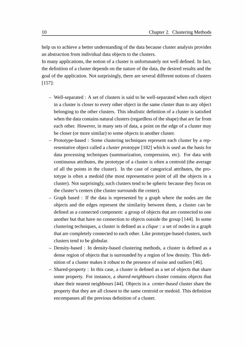
In many applications, the notion of a cluster is unfortunately not well defined. In fact,
the definition of a cluster depends on the nature of the data, the desired results and the
goal of the application. Not surprisingly, there are several different notions of clusters
[157]:
– Well-separated : A set of clusters is said to be well-separated when each object
in a cluster is closer to every other object in the same cluster than to any object
belonging to the other clusters. This idealistic definition of a cluster is satisfied
when the data contains natural clusters (regardless of the shape) that are far from
each other. However, in many sets of data, a point on the edge of a cluster may
be closer (or more similar) to some objects in another cluster.
– Prototype-based : Some clustering techniques represent each cluster by a rep-
resentative object called a cluster prototype [182] which is used as the basis for
data processing techniques (summarization, compression, etc). For data with
continuous attributes, the prototype of a cluster is often a centroid (the average
of all the points in the cluster). In the case of categorical attributes, the pro-
totype is often a medoid (the most representative point of all the objects in a
cluster). Not surprisingly, such clusters tend to be spheric because they focus on
the cluster’s centers (the cluster surrounds the center).
– Graph based : If the data is represented by a graph where the nodes are the
objects and the edges represent the similarity between them, a cluster can be
defined as a connected component: a group of objects that are connected to one
another but that have no connection to objects outside the group [144]. In some
clustering techniques, a cluster is defined as a clique : a set of nodes in a graph
that are completely connected to each other. Like prototype-based clusters, such
clusters tend to be globular.
– Density-based : In density-based clustering methods, a cluster is defined as a
dense region of objects that is surrounded by a region of low density. This defi-
nition of a cluster makes it robust to the presence of noise and outliers [46].
– Shared-property : In this case, a cluster is defined as a set of objects that share
some property. For instance, a shared-neighbours cluster contains objects that
share their nearest neighbours [44]. Objects in a center-based cluster share the
property that they are all closest to the same centroid or medoid. This definition
encompasses all the previous definition of a cluster.

2.2. Clustering evaluation 11
The diversity of cluster definitions is not the only cause of the increasing number of
clustering methods. Features representing the different measures of the properties of
an object are not appropriate for all types of data. The better the choice of the feature,
the more compact the clusters are and a simple clustering algorithm such as K-means
[67] can be used to find them. Unfortunately, no universally appropriate features
seem to exist, the choice of the feature must be related to the domain knowledge, the
purpose of the clustering and the nature of the data set to be clustered.
2.2 Clustering evaluation
How to evaluate the relevance of a clustering result is a central point in any clus-
tering method. For the case of unsupervised clustering, a standard evaluation can be
made when a ground truth is available. The evaluation measure depends on the goal of
the application. While it is possible to develop various numerical measures to assess
the different aspects of the cluster’s validity, there are a number of issues: i) a measure
of cluster validity may be quite limited in the scope of its applicability, ii) we need a
framework to interpret any measure.
A variety of different evaluation measures have been suggested recently in [19, 30]:
– F-measures: introduced by Larsen et al. [101] and combines the precision and
recall measures. It considers that each cluster is the result of a query and that
each class is the desired answer to that query.
– Rand Index: proposed by Hubert et al. [75] to compare two partitions. It can be
used to compare the resulting partition of a clustering algorithm with the ground
truth classes or to compare two partitions resulting from different clusterings.
– Purity: proposed by Zhao et al. [187] to measure the percentage of objects in
a cluster that belong to the largest class of objects in this cluster. The larger the
value of the purity, the better the clustering solution is.
– Cosine Measure: used by [73] and combines the precision and the recall of
each cluster. A low precision score of clustering is an indication of cluster fu-
sion, which often occurs when too few clusters are produced, whereas a low
recall indicates cluster fragmentation, which occurs when too many clusters are
generated. A high cosine measure value can be interpreted that the clustering
avoids extremes fusion and cluster fragmentation, and that the number and sizes
of the clusters roughly conform with those of the classes.

12 Chapter 2. Clustering Methods
All these measures will be described in detail in Section 4.6.1. Recently, a different
way to evaluate clusters has been proposed. Cao et al. [20] present a measure of
the meaningfulness of clusters. This measure is derived from a background model
assuming no class structure in the data. It provides a way to compare clusters, and
leads to a cluster validity criterion. This criterion, inspired by the a contrario approach,
is applied to every cluster. The Helmholtz principle [36] states that if an observed
arrangement of objects is highly unlikely, the occurrence of such an arrangement is
significant and the objects should be grouped together into a single structure. Hence,
clusters are detected a contrario to a null hypothesis or background model (no class
structure in the data). This notion will be used in this PhD to compute the a contrario
significance measures of clusters.
2.3 Data clustering methods
As mentioned above, so many clustering algorithms have been proposed in the lit-
erature, in many different scientific fields and applications, that is would be extremely
difficult to review all the proposed methods. These methods differ in the choice of
data, the objective function, heuristics and hypotheses.
Here, we will not detail all the existing clustering methods. In the next Section 2.3.1,
we present an overview of some clustering methods and the particular properties of
each one. Thereafter in Section 2.3.2, we review some open problems and recent
trends in data clustering. Finally, in Section 2.4, we focus particularly on graph based
methods and especially on spectral clustering and shared nearest neighbours cluster-
ing methods SNN. Our contributions are related to SNN methods and we use spectral
clustering for comparison and positioning.
2.3.1 Overview
Comprehensive surveys on clustering have been published, such as the well-known
papers by Jain et al. [9], Jian et al. [82] and Xu et al. [179] where a large variety of
algorithms are detailed.
One of the most important points that can be helpful in selecting a clustering algorithm
is the nature of the data and the nature of the desired clusters. Data dimensionality and
the size of the dataset are also important criteria since no stable clustering algorithm
exists [47] and might be restricted to low dimensionality [1, 155].
Traditionally, clustering methods are divided into hierarchical and partitioning tech-

2.3. Data clustering methods 13
niques. While hierarchical algorithms are subdivided into agglomerative and divisive,
partitioning algorithms are subdivided into 2 types : i) methods that tend to build
clusters of proper convex shape and look how items fit into their clusters (K-medoid,
K-means, probabilistic clustering), ii) density based methods that define clusters as
high density regions in the feature space separated by low density regions.
The density-based algorithm DBSCAN [46] introduced a frequency count within the
neighbourhood to define a concept of a core point. In fact, while density-based meth-
ods are attractive because of their ability to deal with arbitrarily shaped clusters and
are less sensitive to outliers, they have limitations in handling high-dimensional data.
They are usually used with low-dimensional data of numerical attributes because the
feature space is usually sparse when the data is high-dimensional. This is due to the
fact that it is difficult to distinguish high-density regions from low-density regions in
high-dimension.
To overcome this limitation, subspace clustering algorithms such as CLIQUE [3] try to
find clusters embedded in low-dimensional subspaces of the given high-dimensional
data. When the dimension grows, a problem arises from the decrease in metric sepa-
ration ( curse of dimensionality). Two solutions exist : either reducing the dimension
by transforming the attributes (PCA [128], wavelets [93], Discrete Fourier Transform
DFT [94]) or using clustering techniques for high dimensional data (subspace cluster-
ing [126], multi-clustering techniques [137]).
When the data points are represented by nodes in a weighted graph and the weight
of the edges connecting the nodes represents the pair-wise similarity, the clustering is
referred to graph clustering. The most popular graph clustering is spectral clustering.
The main idea of such clustering is to partition the nodes into subsets such that the sum
of the weights assigned to the edges connecting two subsets is minimized. We detail
spectral clustering techniques in Section 2.4.
2.3.2 Open problems and latest trends in data clustering
While new clustering algorithms continue to be developed, some issues still have
to be resolved. Some problems and research directions as pointed by [76] have to be
addressed:
– There is a need to achieve tighter integration between clustering algorithms and
application requirements. Each application has its own requirements: some of
them just need a global partition of the data while others need to have the best
partition with great precision. Generally, in mining applications, the goal is

14 Chapter 2. Clustering Methods
not to provide all the clusters of the search results but a summarized list of the
different topics of the query. Users can after easily figure out what they are
exactly searching for by selecting the target topic. Showing images from the
target category in which the user is truly interested is much more effective and
efficient than returning all the clusters or all the mixed images.
– There is a need for clustering algorithms that lead to computationally efficient
solutions for large scale data. Not all clustering algorithms can deal with large
scale issues.
– There is a need for stable and robust clustering algorithms that lead to stable
solutions even in the presence of noisy data.
– There is a need to use any available a priori information concerning the nature
of the dataset and the goal/domain of the application in order to decide which
data representation is the most suitable and which clustering method is the most
appropriate.
– There is a need to have generic clustering that can be applied for any type of
data.
– There is a need for benchmark data with available ground truths and diverse data
sets from various domains to evaluate any kind of clustering algorithm because
current benchmarks are limited to a small dataset that can be applied only for a
limited choice of clustering methods.
As said above, the growing amount of data leads to diverse data (both structured
and unstructured). Raw images, text, video are considered as unstructured data be-
cause they do not follow a specific format, in contrast to structured data where there is
a semantic relationship between objects. Generally, clustering approaches are applied
without taking into account the structure of the data. It is precisely for these reasons,
that new algorithms are being developed. Recently, [76] presents an overview of clus-
tering techniques and highlights some emerging, and useful, trends in data clustering,
some of which are presented below :
– Clustering ensembles [58] : The idea here is that by combining multiple parti-
tions (clustering ensembles) of the same data, we can obtain a better data par-
titioning. For example, we can obtain a set of clustering ensembles by taking a
different value of K in a K-means clustering with each time a random initializa-
tion, and then, combining these partitions using a co-occurrence matrix which
results in a good separation of the clusters, as was done in [56]. Applying the
same clustering algorithm with different parameter values is not the only way to
generate a clustering ensemble. We can apply different clustering algorithms on

2.4. Graph-based clustering methods 15
the same data which leads to different clusters or even use different data repre-
sentations of the data with different clustering algorithms.
– Large scale clustering : A number of clustering algorithms have been developed
to handle large size dataset. Some of them are based on efficient nearest neigh-
bours search and use trees as in [119] or random projections as in [16]. Some
others first, try to summarize a large data set into small subset and then apply the
clustering algorithms to the summarized dataset as with the BIRCH algorithm
[186] in contrast to sampling based methods like CURE algorithm [64] which
sub-sample a large dataset selectively and perform clustering over the small set,
which is later transferred to the larger dataset.
– Multi-way clustering [18] When a set of objects to be clustered is formed by a
combination of heterogeneous components, a classical clustering method leads
to poor performances. Co-clustering treats this problem, and has been success-
fully applied to document clustering (clustering both documents and words be-
longing to documents at the same time [38]). This Co-clustering framework was
extended to multi-way clustering in [7] to cluster a set of objects by simultane-
ously clustering their heterogeneous components.
2.4 Graph-based clustering methods
A graph is classically defined by a set of nodes or vertices and a set of edges link-
ing some pairs of nodes. Graphs are a nice way to represent the data when we do no
have more information than the similarity between objects. In this case, the weight
associated to the edge connecting two nodes is equal to the similarity between these
nodes. Graph clustering tends to group vertices of a given input graph into clusters
taking into consideration the edge structure of the graph. Vertices belonging to the the
same group are connected by high weight while edges between different groups have
very low weights.
As the field of graph clustering has become quite popular, the number of clustering
algorithms as well as the number of applications have become high. Graph clustering
algorithms serve as a tool for analysis, model and predict in many different domains
[144]. In social networks for instance, groups of people (such as friends or families)
can be connected by means of their profile as done in collaborative filtering recom-
mendation systems [145].
Representing data by a graph also helps in the biological domain to study for example

16 Chapter 2. Clustering Methods
the spread of epidemics. Newman [120] studied susceptible, infective and recovered
type epidemic processes and found that clustering decreases the size of epidemics.
Generally, the goal of graph based clustering is to group items into clusters such that
connected or similar items are assigned to a same cluster. But each application defines
its own desirable cluster properties. In some applications, the density of edges within
the cluster is more important than the edges with the rest of the graph [86]. Some graph
structures are hierarchical and other graphs can simply computed by flat clustering.
Different kinds of graphs can be computed from a given unstructured set of data items:
– The fully connected graph: Every pair of distinct vertices is connected by a
unique edge. As the goal is to model the local neighbourhood relationships
between items, the edges have to be weighted. The similarity plays the role to
detect partitions with high weights. The choice of the similarity function, used
to compute the weights between objects, is very important for this kind of graph
since all pairs are connected and only the edge weights are discriminant.
– The ε-neighbourhood graph: Only vertices whose dissimilarity is smaller than
ε are connected. The difficulty lies in choosing this parameter. The produced
graph and the resulting clustering are actually very sensitive to the choice of
ε . To determine the smallest value of this parameter, we can consider it as the
length of the longest edge in a minimal spanning tree of the fully connected
graph of the data items. The disadvantage of this method of determining ε is
that if the data contains outliers, this leads to choosing a larger ε , so that some
vertices will be connected even if they are dissimilar.
– The k-nearest neighbours graph: A vertex is only connected to its k-nearest
neighbours. The resulting graph is directed as the nearest neighbour relation is
not a symmetric one, i.e., if an item q is among the k-nearest neighbours of a
point p, this does necessarily mean that p is a nearest neighbour of q. To make
the graph undirected, we can consider that two points are connected if one of the
pair is among the k-nearest neighbours of the other and we ignore the direction
of the edge. A second way is to connect a pair of items only if they are among
the k-nearest neighbours of each other. By this restrictive method, we obtain a
mutual k-nearest neighbour graph which has the property of connecting nodes
within regions of constant density as well as points within different scale of den-
sity. When the clusters are from different densities, this kind of graph is very
useful.
The choice of k is crucial in order to achieve good performances. A small k
makes the graph too sparse or disconnected. On the other hand, by choosing a

2.4. Graph-based clustering methods 17
large k, dissimilar points are related on the graph. The advantage of this kind of
graph is that points belonging to different level of density can be connected. The
similarity function is only used to connect the points to their k nearest neigh-
bours in the graph. [14] suggests guaranteeing the good connectivity of this
graph by choosing k in the order of log(n) with n being the number of the data
items. As for the mutual k-nearest neighbour graph [124], the number of edges
is more limited than for the standard k-nearest neighbour graph and this sug-
gests choosing a large value of k. No theoretical study has clearly resolved the
problem.
– The Bipartite graph: The set of vertices is divided into two subsets and all the
edges lie between these two subsets [177]. Such graphs are natural for many
applications involving 2 types of objects such as documents and words. A word
belongs to a set of documents and at the same time, a document contains a set of
words. The motivation can be to regroup documents having common words. To
achieve this, we simultaneously obtain the clustering of words and of documents.
To evaluate the similarity of two vertices of the same side of the graph can be
done only by evaluating the overlap of their neighbourhood on the other side and
vice versa.
Over the years, there has been a huge amount of work on graph-based clustering [54,
91]. Rather than giving an exhaustive description of all the methods, we focus on two
widely used divisive categories of graph-based methods: “spectral clustering” that is
probably the most well-known one and “shared nearest neighbours clustering” that is
related to our work.
2.4.1 Spectral clustering
Graph-based divisive clustering [51] is a class of hierarchical methods that tends
to divide the graph recursively into clusters in a top-down manner. The division should
not break a natural cluster but rather separate connected clusters from other clusters.
Among this type of clustering, we find the spectral clustering [110] that is very popular
and used extensively in many studies.
The main idea of this clustering is that by computing the eigenvectors corresponding
to the second smallest eigenvalue of the normalised Laplacian, the clustering can be
determined by using the eigenvector as vertex-similarity values.
The success of spectral clustering is mainly based on the fact that it does not need to
have assumptions on the form of the clusters unlike the popular K-means algorithm

18 Chapter 2. Clustering Methods
for example which leads to a convex form of clusters. However, spectral clustering
depends on the choice of similarity graph (choosing the right parameter of connectivity
of the graph representation of items).
A comprehensive tutorial on spectral clustering was given by Ulrike Von Luxburg
[110] and a broad overview of the different methods is available in [166] where an
evaluation of what features make a spectral clustering more valuable is provided.
Spectral clustering as a graph partitioning approach
The goal of graph clustering is to divide data into some clusters such that the el-
ements in the same cluster are highly connected and the edges between the different
clusters have low weights. This means that we aim to separate groups of elements
from each other with the minimum of cuts (often called the min-cut problem) [89].
The clustering problem is then configured as a graph cut problem where an appropriate
objective function has to be optimized.
Let us define by C1,C2, ...,Ck the partition of a data set on k groups that we want to
achieve with the minimum of cuts.
As the objective function that has to be minimized, we can find the normalized asso-
ciation [146], the conductance [87], or the ratio cut [37]. But the most widely used is
the normalized cut (Ncut) [146]:
Ncut(C1,C2, ...,Ck) =k
∑i=1
cut(Ci,Ci)
vol(Ci). (2.1)
where Ci is the complement of Ci and vol(Ci) is the sum over the weights of all the
edges attached to vertices in Ci.
Because spectral clustering techniques have a strong connection with Laplacian Eigen-
maps [8], spectral concepts and graph analysis is the way to solve the relaxed version
of this NP hard problem of the min-cut problem [167, 146].
This relaxation can be formulated by introducing the Laplacian matrix [28]. The re-
sulting balanced groups with low edges between them have another property : a ran-
dom walk (jumping randomly from one vertex to another [107]) on a group stays long
before jumping to another groups. By this property, spectral clustering can also be
interpreted as trying to find a partition that random walks have more chance of staying
on the same cluster than jumping to another cluster. [112] analyse the relation with
the Normalized cut (NCut) and the random walk: when we minimize the Ncut, we are
actually looking for the partition with a frequent random walk within the clusters and

2.4. Graph-based clustering methods 19
hardly from Ci to Ci.
The most popular spectral clustering algorithms are those of [121] and [146]. The core
of these algorithms is the eigenvalue decomposition of the Laplacian matrix L of the
weighted graph obtained from data to solve the relaxed problem of objective functions
like the Ncut. In fact, the second smallest eigenvalue of L is related to the graph cut
[50] and the corresponding eigenvector can cluster together similar items [13, 28, 146].
The main difference between [146] and [121] is the way the normalized graph Lapla-
cian is used.
In the next Section, we describe these two algorithms and some relative properties of
each.
Normalized spectral clustering according to Shi and Malik [146]
This spectral clustering was initially proposed for image segmentation problems
[146]. In the original framework each node is a pixel and the definition of adjacency
between them is suitable for image segmentation purposes. Each pixel of the image
is considered as a point having a feature vector which takes into account several of its
attributes (e.g. intensity, color and texture information). The goal is to regroup similar
pixels describing a same region.
Given a set of points x1,x2, ...,xn of size n, by using the similarity matrix S, we want
to cluster the data into k groups. To do so:
1. construct the affinity matrix A (also called the adjacency matrix) defined by Ai j =
exp(−‖si−s j‖2
2σ2 ) for i �= j and Aii = 0.
2. form the degree matrix D as the diagonal matrix defined by Dii = ∑nj=1 Ai j.
3. compute the unnormalized Laplacian matrix L = D−A.
4. compute the first k eigenvectors v1,v2, ...,vk of the generalized eigen problem
Lv = λDv.
5. form the matrix V containing the eigenvectors as columns elements.
6. consider each row i of V as a point yi and apply K-means algorithm on Y.
7. assign each point xi to cluster j if yi was assigned to the cluster j.
Note that this algorithm uses the generalized eigenvectors of L, hence is called normal-
ized spectral clustering. The next algorithm also uses a normalized Laplacian. As we
will see, this algorithm needs to introduce an additional row normalization step which
is not needed in the other algorithms [110].
20 Chapter 2. Clustering Methods
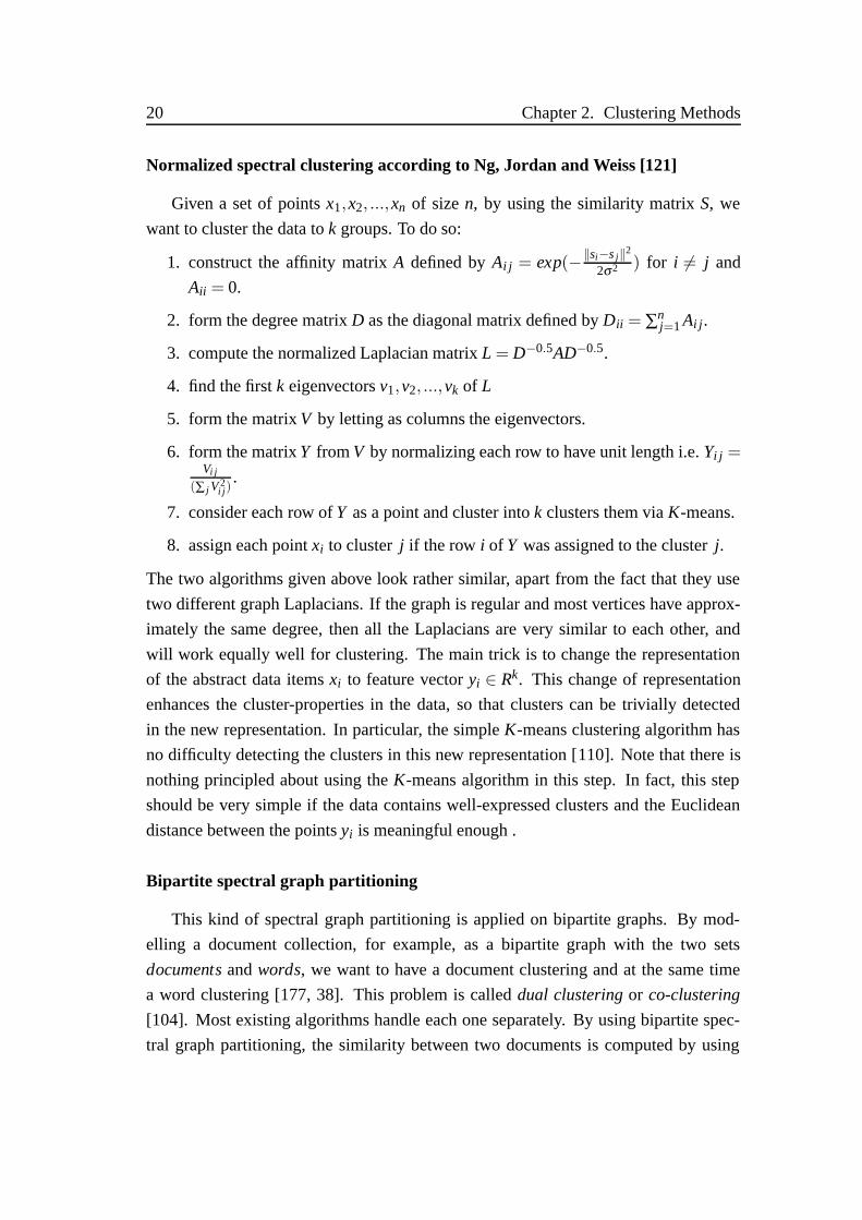
Normalized spectral clustering according to Ng, Jordan and Weiss [121]
Given a set of points x1,x2, ...,xn of size n, by using the similarity matrix S, we
want to cluster the data to k groups. To do so:
1. construct the affinity matrix A defined by Ai j = exp(−‖si−s j‖2
2σ2 ) for i �= j and
Aii = 0.
2. form the degree matrix D as the diagonal matrix defined by Dii = ∑nj=1 Ai j.
3. compute the normalized Laplacian matrix L = D−0.5AD−0.5.
4. find the first k eigenvectors v1,v2, ...,vk of L
5. form the matrix V by letting as columns the eigenvectors.
6. form the matrix Y from V by normalizing each row to have unit length i.e. Yi j =Vi j
(∑ j V2i j)
.
7. consider each row of Y as a point and cluster into k clusters them via K-means.
8. assign each point xi to cluster j if the row i of Y was assigned to the cluster j.
The two algorithms given above look rather similar, apart from the fact that they use
two different graph Laplacians. If the graph is regular and most vertices have approx-
imately the same degree, then all the Laplacians are very similar to each other, and
will work equally well for clustering. The main trick is to change the representation
of the abstract data items xi to feature vector yi ∈ Rk. This change of representation
enhances the cluster-properties in the data, so that clusters can be trivially detected
in the new representation. In particular, the simple K-means clustering algorithm has
no difficulty detecting the clusters in this new representation [110]. Note that there is
nothing principled about using the K-means algorithm in this step. In fact, this step
should be very simple if the data contains well-expressed clusters and the Euclidean
distance between the points yi is meaningful enough .
Bipartite spectral graph partitioning
This kind of spectral graph partitioning is applied on bipartite graphs. By mod-
elling a document collection, for example, as a bipartite graph with the two sets
documents and words, we want to have a document clustering and at the same time
a word clustering [177, 38]. This problem is called dual clustering or co-clustering
[104]. Most existing algorithms handle each one separately. By using bipartite spec-
tral graph partitioning, the similarity between two documents is computed by using

2.4. Graph-based clustering methods 21
their corresponding words, and the similarity between two words is computed by us-
ing the information of documents in which they occur.
Failing to take into consideration the similarity of the words they contain leads to
some problems when we cluster documents and vice-versa: two documents d1 and d2
are considered to be similar because they share a set of words Sw but it can happen that
the words in Sw are never clustered together.
Dhillon [38] proposed a spectral approach to approximate the optimal normalised cut
of a bipartite graph, which was applied for document clustering. This involved com-
puting a truncated singular value decomposition (SVD) of a suitably normalised term-
document matrix, constructing an embedding of both terms and documents, and ap-
plying K-means to this embedding to produce a simultaneous k-way partitioning of
both documents and terms. The usefulness of this approach was however limited and
[97] proposed an adapted bipartite spectral graph partitioning approach to successfully
cluster micro array data simultaneously in clusters of genes and conditions.
Wieling et al. [173] proposed applying a bipartite spectral graph partitioning to a new
sort of data, namely dialect pronunciation data to recognize groups of varieties in this
sort of data while simultaneously characterizing the linguistic basis of the group. Such
a study demonstrates that spectral clustering gives sensible clustering results in the ge-
ographical domain as well as for the concomitant linguistic basis.
Is is not necessarily to have different kind of objects to form a bipartite graph. Si-
multaneous inputs of data from two sensory modalities can be modelled by a bipartite
graph [34]. Each sensory modality is considered as a view and a spectral clustering is
applied to cluster each side while taking the other side into account with the goal of
minimizing the disagreement between the clusterings.
To get a better idea of the principle of bipartite spectral graph partitioning algorithm,
we present here the first one proposed by [38] to cluster documents and words: Given a
set of documents D = d1,d2, ...,dn and a set of words W =w1,w2, ...,wm. We construct
the bipartite graph G = (D,W,E) where E is the set of edges di,wj : di ∈ D,wj ∈W .
By considering the m×n word-by-document matrix A such as Ai j is equal to the edge-
weight Ei j, we want to have a set of word-document dual clusters C = C1,C2, ...,Ck
such that the cut of k-partitioning the bipartite graph is minimized. Minimizing the
normalized-cut is equivalent to maximizing the proportion of edge weights that lie
within each partition such as [146] and [121]. Finding a globally optimal solution to
such bipartite graph partitioning is NP-complete but by using the left and right singular
vectors, we can relax the discrete optimization problem and find an optimal solution.
We present here the bipartite spectral clustering algorithm proposed by Dhillon [38] :
22 Chapter 2. Clustering Methods
1. calculate the diagonal matrices Dw and the Dd of A defined by Dw(i, i)=∑nj=1 Ai j
and Dd( j, j) = ∑mi=1 Ai j
2. form the new normalized matrix of A denoted An = Dw−0.5ADd
−0.5.
3. perform SVD (Singular Value Decomposition) operation on An to obtain the left
and the right k singular vectors Lw and Rd and combine the transformed row and
column vectors to create a new projection matrix Z.
4. run a clustering algorithm as K-means on the Z matrix and return the co-clusters
Cj = (wj,d j), j = 1, ...,k.
Discussion
The main advantage of spectral clustering is that it can transform any graph-based
problem into a linearly separable problem that can be easily solved by an algorithm
such as K-means. Its success is essentially based on the fact that it does not need
strong assumptions on the form of clusters as opposed to K-means where the resulting
clusters have a convex form. Because it is easy to implement and avoids having a
local minima, spectral clustering represents a powerful tool to produce good results.
On the other hand, one drawback of spectral clustering is that it depends on the
type of the graph. [111] demonstrate theoretically and through practical examples
that minimising NCut on a k-nearest neighbour graph leads to different results than
minimising the NCut on a ε-neighbourhood graph. This means that by using a given
data and an spectral clustering algorithm, we obtain different results if we construct
the underlying graph differently and we use different neighbourhood size.
Another critical parameter that has to be fixed is the number of clusters as in most
clustering problems. Guidelines are proposed in the literature such as the ratio of
the intra/inter cluster similarity and many other adhoc measures [100, 55] but there
is a particular one used for spectral clustering based on the eigen-gap heuristic.
Justifications based on spectral graph theory and perturbation theory allow us to
conclude that there is a large gap between the k-th eigenvector and the k + 1-th
eigenvector, which is not the case between the first k eigenvectors where the gap is
very small. In the presence of noise or overlaps between clusters, this heuristic is less
effective: the gap is not significant and the k-th eigenvector cannot be found precisely.
We can conclude that to achieve good results by using spectral clustering, some
parameters have to be considered carefully: the number of clusters, the choice of
graph, and the parameter of connectivity on the graph. Each of these parameters

2.4. Graph-based clustering methods 23
influence consistently the clustering results and is a potential source of instability.
2.4.2 Shared nearest neighbours clustering methods
In this Section, we focus on another kind of graph-based clustering i.e shared near-
est neighbours clustering methods. In these methods, the edge between two nodes rep-
resents the rank of a node in the nearest neighbours list of another node. The rank is
computed using a primary similarity measure that will be discussed in the next para-
graph. Unlike spectral clustering, the goal is not necessarily a global graph cuts op-
timization but a local optimization cut. The use of a similarity based on the shared
nearest neighbours makes the graph less sensitive to the different parameters seen in
the previous section. Let us begin by presenting the effects of high data dimensionality
on a range of popular distance measures and explain why a shared nearest neighbours
measure is more appropriate.
Shared nearest neighbours measure
To support clustering, a measure of similarity or a distance is needed between
data objects but clustering then depends critically on density and similarity. These
concepts become more difficult to define when dimensionality increases. Similarity
measures based on distances are sensitive to variations within a data distribution or the
dimensionality of a data space. These variations can limit the quality of the clustering
solution.
In low dimensions, the most common distance metric used is the Euclidean distance or
the L2 norm. While it is useful in low dimension, it does not work well in high dimen-
sions. One of the reasons is that the Euclidean distance considers missing attributes
to be as important as the present attributes. Often, in high dimensions, data points are
actually sparse vectors and the presence of an attribute has to be more important than
the absence of an attribute.
Even the traditional Euclidean notion of density, which is the number of points per
unit volume, in high dimensional data is meaningless. As the number of dimensions
increases, the volume increases rapidly and if the number of points does not grow
exponentially with the number of dimensions, the density tends to 0. Thus, in high
dimensions, we cannot differentiate between high density regions and low density re-
gions.
To solve this problem, the cosine measure and the Jaccard coefficient were suggested.

24 Chapter 2. Clustering Methods
The cosine similarity between two data points is equal to the dot product of the two
vectors divided by the norm of each vector. The Jaccard coefficient is equal to the
number of intersecting attributes (if the attributes are binary of course) divided by the
number of spanned attributes by the two vectors.
Even if cosine and Jaccard measures can provide relevant similarity measures, they
cannot handle high dimensionality well: there are cases where using such measures
still does not eliminate all the problems of similarity in high dimensions [139]. This
problem is not due to the lack of a good similarity measure but to the fact that in high
dimensions direct similarity cannot be trusted when the similarity between pairs of
points is very low [44].
In fact, [10] demonstrates that in high dimensions, the proportional difference between
the farthest point distance and the closest point distance tends to be equal to 0. As the
dimension increases, the contrast of distance between data points decreases: this is one
of the aspects of the so-called curse of dimensionality [40]. The distance measure does
not become discriminant unless the data is composed of natural well-separated clus-
ters, each one following its own distribution. This is a fundamental problem studied in
detail in [1, 69].
An interesting alternative to direct similarity is to define a secondary measure based on
the rankings induced by a specified primary measure. This primary similarity measure
can be any function that determines a ranking of the data objects relative to the query.
The most basic form of a secondary measure is the similarity between pairs of points
in terms of their shared nearest neighbours SNN.
While we cannot rely on the absolute values of the distance because the curse of di-
mensionality, it is still viable to use distance values to derive a ranking of data objects.
By using a ranking of the nearest neighbours, we are not dependent on the value of
similarity but we retrieve the top k-nearest neighbours independently of their absolute
distance values. In some cases, when dimensionality increases, the ranking improves
significantly [10]. [74] demonstrate that the quality of the ranking may not necessarily
depend on the data dimensionality but on the number of relevant attributes in the data
set. In other words, if the dimensionality increases but the number of relevant attributes
is high, the relative contrast between points tends to decrease but the separation among
different clusters can increase. But if the data dimensionality is high and the number
of relevant dimensions is low, the curse of dimensionality comes into effect. In the
same study, an evaluation of the performance of a secondary similarity measure based
on SNN information is done empirically and compared to the primary distances from
which the rankings were derived. The experiments suggest that using an SNN simi-

2.4. Graph-based clustering methods 25
larity measure can significantly boost the quality of the ranking compared to the use
of the primary distance measure alone. In particular, the secondary distance performs
very well at high dimensionality, and is robust if we respect the neighbourhood size :
for two points from a common cluster, if we consider their neighbourhoods of a large
size but always lower than the real size of the class, the overlap will increase. But if we
use neighbourhoods larger than the size of the class, many others objects from different
groups will be contained in the neighbourhoods of the two points and the performance
of the secondary measure will become less predictable.
Shared nearest neighbours based algorithms
For high dimensional data clustering, traditional clustering algorithms like K-
means, for example, show their limitations to deal with outliers and do not work well
when the clusters are of different sizes, shapes and densities. Agglomerative hierarchi-
cal clustering, known to be better than K-means for low-dimensional data, also has the
same problems. To solve this problem, an alternative similarity based on shared near-
est neighbours was first proposed by Jarvis and Patrick [77]. A similar idea was later
presented in the hierarchical algorithm ROCK [139]. In Jarvis and Patrick’s clustering
method, a graph is constructed as follows: a link is created between a pair of items x
and y if and only if x and y belong to their respective closest k nearest neighbours lists.
The weight of the link can represent the number of shared neighbours between x and y
or a weighted version that takes into account the ordering of the neighbours. All edges
with weights less than a user predefined threshold are removed and all the connected
components in the resulting graph are the final clusters. Defining this threshold is the
major drawback of this method : if the threshold is too high, two distinct sets of points
can be merged into the same group even if there is one link between them. On the other
hand, if the threshold is too small, then natural clusters can be split into many small
clusters. Despite this drawback, this algorithm presents some advantages: noise points
and outliers will have their link broken because they are not in the nearest neighbours
lists of their own neighbours. Uniform regions will keep their links until transition
regions break the ones (we can say that the graph is independent of the density of the
regions, only links are important).
For low to medium dimensional data, density-based algorithms such as DBSCAN [46]
have been proposed to find clusters of different sizes and shapes but not of different
densities. This method introduced the idea of representative or core points that be-
come the origin of the clusters. In DBSCAN, the density associated with a point is

26 Chapter 2. Clustering Methods
obtained by counting the number of points in a region of a specified radius around the
point. Points with a density higher than a specified threshold are considered as core
points and clusters will grow around these points. In this way, this method can find
clusters of different shapes but not of different densities. For this reason, an SNN clus-
tering algorithm [44] was proposed to deal with this problem by using a density based
approach to find core points: by computing the sum of links strengths for every point
in the SNN graph, points that have high total link strength then become candidates for
the representative core points, while the others become noise points.
It is not difficult to see that there are many disadvantages of this method: the defini-
tion of thresholds for core points and outliers is not clearly provided (core points may
belong to identical clusters while core points had better be as disperse as possible).
The performance of the SNN greatly depends on the tuning of several non-intuitive
parameters specified by the user and it is difficult to determine their appropriate values
on real datasets.
In conclusion, a common need of the previous shared neighbours algorithms is that a
fixed neighbourhood size (in terms of the number of neighbours k as in Jarvis-Patrick
and SNN or in terms of the radius r of the neighbourhood in ROCK or DBSCAN) has
to be chosen in advance by the user and applied equally to all items of the dataset to
cluster which leads to bias in the clustering process.
Recently, an SNN-based clustering method was proposed by Houle [73] that allows the
variation of the neighbourhood size. The Relevant Set Correlation (RSC) model de-
fines the relevance of the data point x to a cluster C in terms of the correlation between
items in C with the |C|−nearest neighbours set of x. The model does not require the
user to choose the neighbourhood size or to specify a target number of clusters. The
clustering process is not guided by a global optimization criterion but by only a local
criterion for the formation of cluster candidates. For each item, an optimal radius that
maximizes the quality of the cluster is selected. A greedy strategy is then applied to
keep the clusters according to their qualities and their overlap with the other clusters.
In this work, we provide several contributions and insights into SNN clustering by
firstly revisiting shared nearest neighbours metrics using the a contrario approach, then
we extend SNN approach to the multi-source case and finally to the bipartite case. For
each case, theoretical contributions and experimental applications are provided. We
will focus particularly on visual content which seems an interesting application of our
method. For this reason, in the next Chapter, we provide a short overview of visual
content structuring and mining techniques.

Chapter 3
Visual Content Structuring andMining
The steady growth of the Internet, the falling price of storage devices and an in-
creasing pool of available computing power make it necessary and possible to ma-
nipulate very large repositories of digital information efficiently. Analysing this huge
amount of multimedia data to discover useful knowledge or even just browse is a chal-
lenging problem. The task of developing data mining methods and tools is to discover
hidden knowledge in unstructured multimedia data. The data is often the result of
different outputs from various kinds of information sources, each one with its own
modality. The fact of organizing, searching, managing, clustering and more generally
structuring helps to improve decision making. These tools have been applied in dif-
ferent domains such as medical data, news, consumer purchasers of a store as well as
user generated contents (UGC).
The typical data mining process consists of several stages and the overall process is
inherently interactive and iterative. The main stages of the data mining process are
[48]: (1) Domain understanding; (2) Data selection; (3) Data preprocessing, cleaning
and transformation; (4) Discovering patterns; (5) Interpretations; and (6) Reporting
and using discovered knowledge [127].
At the heart of the entire data mining process lies pattern discovery. This includes
clustering, classification and visualization. Summarizing a huge amount of data so as
to be able to browse it is not a trivial task.
Many intelligence agencies and low enforcement bodies now employ this technology
to fight against child pornography, the trafficking of cultural objects and counterfeit-
ing. Various fields ranging from Commercial to Military want to analyse data in an
efficient and fast manner.
28 Chapter 3. Visual Content Structuring and Mining
In this PhD, we particularly interested in “visual contents mining” which is a complex
domain with different challenges that are sometimes specific to images [95]. Visual
mining is not just an extension of data mining to image domain. It deals with the ex-
traction of hidden knowledge, image data relationships, or other patterns not explicitly
stored in the images. The goal is to determine how low-level pixel representations
can be processed to identify high-level objects and relationships. For example, many
pictures of various persons once stored and mined can reveal interesting images of
the same music concert because some patterns have been detected and shared in these
collections of data. Clearly, visual contents mining does not aim to extract and/or to
understand features from images but to discover and to extract significant visual pat-
terns in a collection of visual documents such as images, videos, etc.
We will not review all the problems here but focus on the following issues related to
the applicative experiments of our work in this PhD: (1) Browsing and summariza-
tion; (2) Building visual vocabularies; (3) Visual object discovery; (4) Multi-cue and
multi-modal image clustering.
3.1 Browsing and summarization
There has been a wide variety of innovative ways to browse and summarize multi-
media information from the visual content. The first idea was to cluster visually simi-
lar images in the same cluster and then convert image clusters to a video in sequential
order based on their inter-cluster similarities. Image cluster contents can be viewed
separately by selecting an index frame from the global overview and by showing a
video loop of cluster frames in a minimum variance order [154]. Hari Sundaram et al.
[156] presented a novel framework for condensing computable scenes. The solution
consists in analysing visual complexity and film syntax, then robust audio segmenta-
tion and significant phrase detection via SVM’s and finally determining the duration
of the video and audio segments via a constrained utility maximization. The aim is to
make the user able to have an abstract of the story in video format.
For summarising video, Snoek et al. [153] propose grouping by categories and brows-
ing by category and in time. [175] group similar images and explore the use of a
nearest neighbour network to facilitate interaction with the users.
All these solutions, at some point require a clustering phase based on different visual or
multi-modal features. For more details, the readers can refer to the interesting survey
[103].

3.2. Building visual vocabularies 29
3.2 Building visual vocabularies
The visual vocabulary is a strategy issued from the text retrieval community. A
document is a distribution of words and all the different tasks related to a document
such as indexing, retrieving documents in which a query word exists, can be done with
relevant results. By considering an image as a visual document, we can consider local
features descriptors as visual words. A feature vector can be expressed in terms of the
region of the feature space to which it belongs. Each visual document is represented
by a distribution of visual words (BOW) over a fixed vocabulary. Work on object based
image retrieval [151] has imitated simple text-retrieval systems using the analogy of
“visual words”.
The building of a standard visual vocabulary consists in:
– Collecting a corpus of images and selecting a set of features: The most accurate
results are generally obtained when using the same data to create the vocabulary.
Generally, the goal is to construct a generative vocabulary with a corpus and this
vocabulary has to deal with any other data and not be an application-specific
vocabulary. For this purpose, [125] proposed collecting images from WWW
clustering them and eliminating irrelevant ones.
– Clustering the sampled features in order to quantize the space into a discrete
number of visual words. Usually, a simple K-means clustering is used [88]. The
number of clusters has to be given as user-supplied parameter and the centers
of the clusters represent the visual words. The problem is that the size of the
data essentially rules out methods such as mean-shift, spectral and agglomera-
tive clustering. It is true that K-means clustering is effective but it is difficult
to scale to large vocabularies. Some work [42] has been done on accelerat-
ing the k-means but it requires O(K2) extra storage, where K is the number of
cluster centers, rendering it impractical. More recent work has used cluster hi-
erarchies [115] and greatly increased the visual-word vocabulary size by using
them. [122] generates a “vocabulary tree” using a hierarchical K-means cluster-
ing scheme where a branching factor and number of levels are chosen and then
hierarchical K-means is used to recursively subdivide the feature space. Philbin
et al. [132] propose scaling K-means to a large vocabulary using of approximate
nearest neighbour methods. The method has similar complexity to the vocabu-
lary tree, but far superior performance.
Another problem to take into account is the size of the vocabulary. It has been

30 Chapter 3. Visual Content Structuring and Mining
observed in [31, 85, 129] that even with databases containing a limited number
of categories, the best performances are obtained with a large vocabulary. Be-
cause the cost of histogram computations depends on the size of the vocabulary,
one way to reduce the computational cost is to have a more compact vocabulary.
Winn et al. [174] studied the problem of defining and estimating descriptive
and compact visual models of object classes for efficient object class recogni-
tion. They proposed an approach based on the information bottleneck principle
(a technique introduced to find the best trade-off between accuracy and com-
plexity) [159]. A vocabulary inatially containing several thousand words was
reduced to 200 words without any lose of performance. A tree structure, as the
Extremely Randomized Clustering Forests, was also proposed in [117] to organ-
ise the vocabulary with the goal of reducing the computational cost.
In short, building a visual vocabulary depends on the type of visual features, the input
set of features, the number of words to be selected and the type of clustering algorithm.
The lack of geometry in BOW can be both an advantage or a disadvantage. By count-
ing only the occurrence of visual words and not considering the relative geometry,
we obtain a flexibility to variation (view point, pose changes). At the same time,
the geometry between features can represent a discriminant factor. Furthermore, by
incorporating a post processing spatial verification step [132] or by considering the
neighbourhood of words, one can achieve a better representation of the geometry.
Given a new image, each local feature region is assigned to the nearest visual word.
Thus, the image is represented with a list of words number. Such representations are
equivalent to standard vector-space models in text information retrieval allowing to
efficiently measure the similarity between items with classical operators. Such simi-
larities only consider global statistics of the image which is a problem when the goal
is to discover very small objects representing a small part of an image.
When dealing with small objects, the solution is to use a method based on probing
local query regions. Many studies [132, 78] use this second type of strategy and con-
sider each local feature of an image independently. Joly et al. [84] show that using
each local feature is effective in retrieving small objects, such as trademark logos.
The disadvantage of this accurate local description of image strategy is that the number
of candidate local regions can be huge. Even with the most efficient indexing struc-
tures that drastically reduce the computational costs, the overall complexity remains
expensive.
Chum et al. [27] propose automatically selecting Regions Of Interest (ROI) with a
very low computational cost. Their method combines BOW models with a geometric

3.3. Visual object discovery 31
Min-Hash [15] and can be considered as a trade-off between global and local strate-
gies.
Adopting another solution to avoid querying all possible regions of interest while keep-
ing a good coverage of the contents, Letessier et al. [102] propose a weighted and
adaptive sampling strategy aiming at selecting the most relevant query regions. A
concept of consistent visual words is proposed and the experiments demonstrate that
these consistent visual words largely overcome the usual visual words and are very
effective to describe and retrieve local visual contents. To generate consistent visual
words (CVW), they developed a framework based on Adaptive Sampling and Priors.
The core idea is that the visual vocabulary produced by an adaptive sampling method
might be adapted to what the user is searching for. A CVW is a set of image patches.
These patches are described by local feature sets. A CVW models a small rigid object,
or a piece of a bigger object and is defined by the geometric consistency between the
feature points of the patches considered. In Section 8.1, we propose a visual objects
discovery and object-based visual query suggestion based on this method.
While there are studies on supervised refinement of visuals words [113, 118], Ron-
grong et al. [81] propose using correlative semantics labels to guide the quantizer in
building more semantically discriminative codewords. By using Hidden Markov Ran-
dom Field, they generatively model the relationships between correlative Flicker labels
and the local image patches to build a supervised vocabulary.
Concerning the multi-modal side of a vocabulary, very little work has been carried out
on multi-modal or multi-cue vocabularies [106]. Shared nearest neighbours methods
introduced in this PhD could help to build such vocabularies.
3.3 Visual object discovery
The success of data mining techniques in semi-structured data (e.g. xml data) has
generated interest in applying them to many computer vision tasks : object retrieval
[149], categorization [168], object discovery [135, 160]. To discover visual objects,
tools from the statistical text analysis community have been borrowed [150]. All the
methods using these tools generally start from the same image representation: they ex-
tract some local visual primitives (interest points [109] or regions [114]) and consider
their “visual words” as input to text-based data mining. The image is then described
in terms of a set of quantized local image patch descriptors. The images are treated as
documents, each image being represented by a “bag of words”.

32 Chapter 3. Visual Content Structuring and Mining
One major issue highlighted by [138], is that “visual words” are not always as descrip-
tive as their text counterparts. Visual words do capture high-level object parts as well
as many others encoding simple oriented corners. Consequently, there is ambiguity
regarding two aspects: synonym and polysemy. A synonymous visual word describ-
ing the same object or object part, and, more problematically, the polysemous visual
word mean different things in different contexts. One way to reduce the ambiguity of
polysemous visual words is to consider the spatial context. Indeed, all visual words in
an image are generally embedded into a single histogram, losing all spatial and neigh-
bourhood relationships. This could provide further improvement. We revisit this later.
Probably, the first work that studied the problem of object discovery is [172]. They
presented ideas for learning mixture models of objects from unhomogeneous training
images in an unsupervised setting. In their work, distinctive features of the object class
are selected automatically and the joint probability density function encoding the ob-
ject’s appearance is learnt. This allows the automatic construction of an object detector
which seems robust to clutter and occlusion.
Thereafter, probabilistic models interested several authors. Sivic et al. [147] proposed
a model developed in the statistical text literature: probabilistic Latent Semantic Anal-
ysis (pLSA) [71]. In text analysis, this is used to discover topics in a corpus using
the bag-of-words document representation but in the context of images, they consider
object categories as topics. Thus, an image containing instances of several categories
is described as a mixture of topics like a term-document occurrence matrix with clas-
sical models used in text-based information retrieval. [105] extend the PLSA model
with the integration of a temporal model to discover objects in a video. Others such as
[12, 158, 170] use another Latent Topic Models : Latent Dirichlet Allocation (LDA)
or hierarchical LDA [148].
The idea underlying these methods is to use common Bags-of-visual-Words models
(BOW) and to analyze the resulting term-document occurrence matrix with classical
models used in text-based information retrieval. Some object discovery methods such
as [170, 161] started by including spatial information to improve their results. Also,
the method of [133] makes a step forward by augmenting the topics of the LDA model
with the spatial position of the visual words. Latent topic models are a favourite choice
for object category recognition and retrieval. But their generalization ability is rather
a disadvantage when searching for particular object instances. The underlying models
tend to be dense rather than sparse and fail to discover accurate clusters of object in-
stances.
Most other methods rely on graph-based clustering methods. The majority of these

3.3. Visual object discovery 33
methods are based on two steps: matching graph construction, and analysing this
graph.
To build a matching graph, they need to discover an object’s seeds, i.e. spatially stable
image regions in the collection. Nodes of the matching graph typically represent im-
ages whereas edges correspond to common matching regions between the images.
A method that combines BOW models with a Min-Hash hashing scheme [15] is pro-
posed by [26, 27] and has a very low computational cost. The MinHash scheme may
be seen as an instance of locality sensitive hashing, a collection of techniques for using
hash functions to map large sets of objects down to smaller hash values in such a way
that, when two objects have a small distance to each other, their hash values are likely
to be the same. Applied on visual words, it can efficiently discover very discriminant
candidate visual sketches that are likely to be parts of more reliable objects.
The drawback of this method is that it does not deal with small objects, as pointed out
by [25] who proposed a new Min-Hash based strategy called Geometric Min-Hash.
This version is able to discover more relevant local sketches and is therefore a very
efficient way to discover candidate query regions that are likely to contain object in-
stances.
Once the matching graph has been constructed, graph-based object mining methods
differ in the way they analyse or post-process the graph. One of the simplest operations
for splitting a graph is to find connected components as proposed in [134, 24, 4]. How-
ever, as pointed by [134], the main problem is that many disjoint objects are grouped
in the same component due to under-segmentation.
Grauman et al. [63] propose a method based on spectral clustering. They aim to sep-
arate the objects from the background and propose a semi-supervised extension. A
great disadvantage of spectral clustering is the need to specify the number of clusters,
whereas in some cases it is impossible to know a priori how many objects could be
found.
More recently, [134] also used a spectral clustering approach but in the context of spa-
tially verified objects. They automatically estimate the optimal number of clusters by
performing multiple clustering, leading to a consistent cost overhead. Furthermore, the
clusters produced suffer from over-segmentation and therefore require some additional
heuristics to merge them into consistent clusters.
Tuytelaars et al. [163] evaluated the performance of different unsupervised methods
of object discovery based on bag-of-visual words image representation. The authors
conclude that to maximize the performance, it is important to select the right image
representation (interest points, dense patches, or both). They also conclude that cor-

34 Chapter 3. Visual Content Structuring and Mining
rectly normalizing the bag-of-words histograms is also important in order to improve
results. Moreover, these design choices are different for latent variables models than
for spectral clustering based methods.
In this PhD, we introduce an alternative object discovery method based on our shared
nearest neighbours clustering algorithm and consistent visual words [102].
3.4 Mono-source, multi-cue and multi-modal imageclustering
3.4.1 Web image clustering
In the beginning, clustering and classification received less attention than feature
extraction and similarity computation of images. With the explosion in the growth
of the World Wide Web, the public has been able to gain access to massive amounts
of information, and the need for practical systems to manage this data has become
crucial. For example, in response to the user’s query, current image search engines
return a ranked list of images and present them as a sorted thumbnail grid (up to 1
million images).
For this reason, it is usually difficult to identify the specific images which the user is
interested in. Users are forced to sift through a long list of images. Moreover, internal
relationships among the images in the visual search result are rarely presented and
are left up to the user. One of the alternative approaches is to automatically group
the search results into thematic groups (clusters). The display groups similar images,
enabling users to quickly scan for the most relevant images. This visualization allows
users to exploit the location of images and to use thumbnails to preview potentially
relevant images.
The problem is the same when a user has a personalized collection of heterogeneous
images that he wants to structure into groups of similar images which facilitates
archiving and retrieval of large image repositories. Browsing and the searching
become easier and more efficient.
Web images have received particular attention from the multimedia community, and
the reader may refer to these studies for comprehensive reviews: [171, 57, 17, 32].
Classifying images with complex scenes is a challenging task because of the variabil-
ity of illuminations, scale condition, geometric transformation, etc. The availability of
image annotations makes them advantageous compared to unlabelled images.
In [61], the authors discuss how to apply appropriate processing to different types of

3.4. Mono-source, multi-cue and multi-modal image clustering 35
images (landmark images and images coming from webcams) and to decide which
clustering and classification approaches are appropriate.
3.4.2 Multi-cue and multi-modal image clustering
There are different kinds of media on the WWW, including text, images, videos,
and audio. Unfortunately, most existing search engines support only one type of
media, and little work has been done on integrating different kinds of media in
the same framework. In 2006, among the major research challenges cited in the
state-of-the-art and challenges of content-based multimedia information retrieval of
[103] (and declared before in 2004 in [95] as an issue to be studied), we can quote:
“Multi-modal analysis and retrieval algorithms especially towards exploiting the
synergy between the various media including text and context information”.
An image has many properties which are quite different from one information source
to another. Relying purely on the keywords around the images produces a lot of noise
in the search result. One possible solution is to benefit from all available sources of
information which might help to have more meaningful information concerning the
images. By considering all information sources as simple oracles returning ranked
lists of relevant objects, we can carry out a multi-modal analysis and clustering
towards exploiting the above-mentioned synergy between the various media including
text and visual information or between any other sources of information.
Multi-modal mining tends to combine different features or to generate more semanti-
cally meaningful features.
The healthcare industry, for example, is producing massive amounts of multi-modal
data : Wang et al. [168] present a new multi-modal mining-based clinical decision
support system that brings together patient data captured in various way to provide a
holistic presentation of a patient’s exam data, diseases, and medications. In addition, it
offers a disease-specific similarity search based on various data modalities to assemble
statistically similar patient cohorts summarizing possible diagnoses, their associated
medications,and other demographic information. The key idea explored is that by
finding similar patients based on a disease-specific analysis of their raw data, they can
make inferences about similarities in their diagnosis and hence their treatments and
outcomes.
[33] is an overview of technologies that support media retrieval in a way that is
complementary to visual analysis. Authors aim to emphasize that technology based

36 Chapter 3. Visual Content Structuring and Mining
on linguistic and contextual sources can bring more than basic keyword search in
collateral text. They illustrate how linguistic, knowledge-based, and visual resources
can be combined to detect high-level concepts, and how contextual information can
improve retrieval results obtained via visual analysis.
The issue for multi-modal data mining is how to merge the different features. The
classifiers can run either on concatenated feature vectors coming from the different
available modalities or by combining the result of multiple classifiers on each modality
to make a final decision. The first option is usually not recommended due to the curse
of dimensionality, there is a need for an efficient way to apply mining techniques on
multi-modal data while keeping the correlation among different modalities intact. The
second option has to apply a relevant fusion in order to have a successful result. In
this approach, by processing each modality separately, we discard the inherent associ-
ations between different modalities. [143] demonstrate the effectiveness of combining
three multi-modal classifiers. They model the problem of combining classifiers as
a reclassification of the judgement made by each classifier. The experiments show
that they obtain better results than the traditional approaches like “majority voting” or
“linear interpolation” because these two methods ignore generally the relative quality
among the classifiers.
The problem of combining different classifiers, each one with its own modality, is that
generally the synergy between the modalities is not exploited as done in [180] where
common sources of spam images are revealed by a two-level clustering algorithm. At
the first level, they calculate visual similarities between images and similar images
are grouped into some clusters. At the second level, the textual similarities between
images is calculated to refine the clustering results from the first level. Exploiting
some mining algorithm based on association rule could enhance the effectiveness of
the results obtained [11].
Chen et al. [23] propose a decision tree-based multi-modal data mining framework for
soccer goal detection from soccer videos because different modalities have different
contributions to the soccer goal detection application domain.
In [116], the authors propose a method for extracting meaningful and representative
clusters that is based on a shared nearest neighbours (SNN) approach. They treat
both content-based features and textual descriptions (tags) but they produce two sets
of clusters (an image could be an element of a tag-based cluster and a content-based
cluster). By displaying the two cluster sets with their representative form, users can
browse a cluster and switch from one cluster set to another. When they combine the
two clusterings (by a simply summing the visual and textual similarity matrix), they

3.4. Mono-source, multi-cue and multi-modal image clustering 37
lose the particularities of each modality and produce clusters that are more ambiguous
and hardly understandable by a user.
[17] propose three representations of web images (visual, textual and link information)
and apply spectral techniques to cluster the search results into different semantic
categories. In [141], the authors address the problem of web image clustering by
simultaneous integration of visual and textual features from a graph partitioning per-
spective. They propose a CIHC (Consistent Isoperimetric High Order Co-clustering)
framework. More recently, [39] have organized image search results by a hierarchical
clustering based navigation. First, the K-lines based semantic clustering organization
is applied. Second, the resulting images corresponding to each phrase are clustered
with the Bregman Bubble Clustering (BBC) algorithm. Bekkerman et al. [7] develop
an effective multi-modal clustering using the Combinatorial Markov Random Field.
They allow more flexibility in their approach (the modalities are not fixed, there is
no limitation in the number of modalities and they take into account other modalities
which do not have to be clustered).
Sabrina Tollari et al. [162] studied how to automatically exploit visual concepts in
an image retrieval task. Authors use Forest of Fuzzy Decision Trees (FFDTs) to
automatically annotate images with visual concepts and show that automatic learning
of visual concepts and then its exploitation, by filtering of text-based image retrieval
is effective.
Recently, Young-Min et al. [96] proposed a new multi-view clustering method
which uses clustering results obtained on each view as a voting pattern in order to
construct a new set of multi-view clusters. The proposed approach is an incremental
algorithm which first groups documents having the same voting patterns assigned by
view-specific PLSA (Probabilistic Latent Semantic Analysis) models [72]. Working
in the concatenated feature spaces, the remaining unclustered documents are then
assigned to the groups using a constrained PLSA model.
Generally in the state-of-the-art of multimedia data mining, studies do not pay
attention to the accuracy of sources. In some cases, a feature of a modality can be
extracted with some errors due to the semantic gap or to the breakdown of the source
of the information that produces the feature. We need a way to make multi-modal
fusion accurate and robust against noisy or near random source of information.
Most previous work on multimedia clustering has focused on specific modalities but
not on the genericity and the robustness of the clustering algorithm itself when it is
used in a multi-source approach.

38 Chapter 3. Visual Content Structuring and Mining

Part II
Contributions to shared nearestneighbours clustering


Chapter 4
Revisiting shared nearest neighboursclustering
4.1 Introduction
Unsupervised data clustering remains a crucial step of many recent multimedia re-
trieval approaches, e.g. web objects and events mining [136], search results clustering
[92] or visual query suggestion [185]. However, the performance and applicability of
many classical data clustering approaches often force particular choices of data rep-
resentation and similarity measures. Some methods, such as k-means and its variants
[90], require the use of Lp metrics or other specific measures of data similarity; others,
such as the hierarchical methods BIRCH [186] and CURE [64], pay a prohibitive com-
putational cost when the representational dimension is high, due to their reliance on
data structures that depend heavily upon the data representation. Such assumptions are
particularly problematic in a multimedia context that usually involves heterogeneous
data and similarity measures.
An interesting alternative approach to clustering that requires only comparative tests
of similarity values is the use of so-called shared-neighbours information [77, 70, 181,
45, 139, 73] as discussed in chapter 2. Here, we present our first contribution to the
clustering paradigm : we introduce a new SNN formalism based on the theory of a
contrario decision. This allows us to derive more reliable connectivity scores of the
candidate clusters and a more intuitive interpretation of locally optimum neighbour-
hoods.

42 Chapter 4. Revisiting shared nearest neighbours clustering
4.2 Basic principles, Notations and Definitions
The basic principle of SNN clustering methods is to consider that a perfect cluster
is composed of items that have their all neighbours in the same cluster. Two elements
are considered involved, not in relation to their similarity value but rather by the degree
of similarity of their respective neighbours. This means that if two elements have a
high proportion of neighbours in common, it is reasonable to put them in the same
group. The advantage is that no hypothesis is made on the shape, density or metric.
Figure 4.1 illustrates this in the Euclidean space. It shows four clusters of different
size, density and shape. With most clustering methods, these clusters would have
different significance measures but according to the principles of shared neighbours
clustering methods, all the clusters are considered to be perfect clusters. Every item in
each cluster has its all neighbours in the same cluster. Let us consider in the following,
Figure 4.1: Four clusters of different size, shape and density considered as perfectclusters in shared neighbours clustering
a set X of N items from some domain D. The feature of these elements can be of any
type. We assume the existence of a function FK that associates to any item x from X its
K nearest neighbours with respect to some similarity or distance measure. Notice that
this metric might be totally unknown. Only the ranking it produces is known.
Let us denote as nnk(x) ∈ X the k-th nearest neighbours of x ∈ X with respect to some
distance metric. The Fk is defined as:
Definition 1. K-nearest neighbours function FK:

4.3. a contrario SNN significance measures 43
FK(x) = {nnk(x)|0 < k ≤ K}For any i < j , the item nni(x) is more relevant or similar to x than nn j(x).
We sometimes refer to FK as an oracle or an information source that returns a
ranked list of relevant items to a query. During this work, we will consider a few
different kinds of oracles. Since no hypothesis is made on the nature of the items or the
similarity metric used to compare items between each other, we define the similarity
between a pair of items x1 and x2 in terms of their shared nearest neighbours. That is
the intersection between their K-NN :
Sim(x1,x2) = |FK(x1)∩FK(x2)|. (4.1)
But though the initial metric and the shared neighbours similarity are both used for
similarity assessment, they do not share the same fundamental properties. Metrics
(sometimes called distance function or simply distance) satisfy four basic properties:
– non-negativity: d(x,y) ≥ 0
– identity: d(x,y) = 0 if and only if x = y
– symmetry: d(x,y) = d(y,x)
– triangle inequality: d(x,z) = d(x, y) + d(y, z)
Shared neighbours similarity is non-negative and symmetric, however it does not re-
quire to satisfy the triangle inequality. In addition, the fact that two items x1 and x2
have elements in common, does not necessarily mean that x1 belongs to the K-NN of
x2 and vice versa.
4.3 a contrario SNN significance measures
4.3.1 Raw SNN measures
The primary shared neighbours similarity measure of any set A ⊂ X is defined
similarly to [73] as :
Definition 2. Intra-significance measure :
I(A) =1|A| ∑
x∈A
(A∩F|A|(x))
=1|A| ∑
x∈A
IA(x) (4.2)

44 Chapter 4. Revisiting shared nearest neighbours clustering
Intuitively, I(A) measures the average number of common neighbours between
A and the |A| nearest neighbours of any of its items. Unfortunately it has the
disadvantage of a bias related to the size of the set. When the size of the set is large,
it is much easier to achieve a high value by chance than when the size of the set is
small. This can be easily illustrated by a short synthetic experiment. Let us consider
an initial set of 100 items denoted as x100. We produce 10000 random subsets of items
of different sizes from x100 and we use a random oracle to produce a random list of
nearest neighbours in x100 for each item of the subsets.
As this notion of random oracle will be re-used many times in this PhD, we define it
here formally.
Definition 3. Random Oracle :
Given a dataset X composed of N items , we define a random oracle RK(x) as a function
returning K items selected uniformly at random from X for each item x.
Figure 4.2: Illustration of the intra-significance measure I(A)
Figure 4.2 shows how the intra-significance measure increases when the size of the
cluster increases. When the size of the cluster size approaches that of the dataset (100
items) the intra-significance measure reaches its maximum value and is equal to the
size of the cluster.
To compare two sets with different sizes, we need to find a way to remove this bias.

4.3. a contrario SNN significance measures 45
4.3.2 a contrario normalization
To remove the bias of the raw measure, we propose using the a contrario principle
[35]. Such a contrario normalization has already been proposed for clustering
[20, 165], but not for SNN. The a contrario approach is a mathematical formalization
of a perceptual grouping principle. The more a set of objects is highly unlikely, the
more the occurrence of such an arrangement is significant and the more the objects
should be grouped together into a single group. Clusters are detected a contrario to
a null hypothesis or background model. The meaningfulness of a group of objects is
measured by the number of false alarms (N f a) that would have been produced under
the null hypothesis. The lower the N f a is, the more significant the group is considered
to be. This measure is used for example in [20] to rank clusters and to decide whether
a cluster is a natural group in which outliers have been discarded.
Let us call H a null hypothesis where a list of neighbours is produced by a random
oracle, i.e. generated by means of uniform random selection from the available items.
Under this null hypothesis, the number of shared neighbours IA(x) between a set A ⊂ X
and the |A| nearest neighbours of an item x selected uniformly at random from X is a
hypergeometrically distributed random variable with expectation:
E[IA(x)] =|A|2N
(4.3)
and variance:
Var[IA(x)] =|A|2(|N|− |A|)2
N2(N −1)(4.4)
Deriving the formal distribution of the intra-significance measure I(A) is unfortunately
a tricky task. But we can approximate it thanks to the central limit theorem. This theo-
rem says that the mean of a sufficiently large number of independent random variables,
each with finite mean and variance, will be approximately normally distributed [142].
By applying this theorem, we can assume that the measure I(A) follows a normal dis-
tribution N (μA,σ 2A) with:
μA = E[I(A)] = E[IA(x)]
=|A|2N
(4.5)

46 Chapter 4. Revisiting shared nearest neighbours clustering
and
σ 2A = Var[I(A)] =
|A||A|2 Var[IA(x))]
=|A|(N −|A|)2
N2(N −1)(4.6)
As it is possible to relate all normal random variables to a standard normal, we can
standardize the normal distribution I(A) to a normal distribution function with expec-
tation 0 and variance 1.
We can therefore define a new shared-neighbour measure Z as:
Z(A) =I(A)−E[I(A)]√
Var[I(A)]
=
√N2(N −1)√
|A|(N −|A|)2(I(A)− |A|2
N)
=√|A|(N −1)
N|A|(N −A)
(I(A)− |A|2N
) (4.7)
With expectation:
E[Z(A)] =√|A|(N −1)
N|A|(N −A)
(E[I(A)]− |A|2N
)
= 0
and variance:
Var[Z(A)] = Var[√|A|(N −1)
N|A|(N −A)
(I(A)− |A|2N
)]
= (√|A|(N −1)
N|A|(N −A)
)2Var[I(A)]
= 1
Directly using this standardized measure rather than the I measure would be equiva-
lent to what Houle [73] called a ”standard score” expressed in terms of the Pearson
correlation:
ZHoule(A) =√|A|(N −1)SR1(A) = Z(A) (4.8)
Where SR1(A) is the expected correlation between A and the relevant set of size |A|based at randomly selected items of A:
SR1(A) =1|A| ∑
x∈A
RHoule(A,F|A|(x)) (4.9)

4.3. a contrario SNN significance measures 47
and a normalised set correlation R defined as:
RHoule(A,B) =| A∩B | −|A||B|
N√| A || B | (1− |A|
N )(1− |B|N )
(4.10)
It is in favour of this method that the same result can be obtained from another method-
ology (a contrario). But, we can still go a step further in our a contrario model.
Now that we have estimated the distribution of our intra-significance measure Z under
the null hypothesis H, we can estimate the precision score a contrario to H as follows:
PZ(A)(z) =∫ z
−∞
1√2Π
e−t22 dt
= 1−φ(z) (4.11)
Where φ() is the cumulative distribution function of the standard normal distribution
that describes probabilities for a random variable to fall within the interval ]−∞,z].
PZ(A)(z) is the probability that Z(A) does not exceed a threshold z under the null hy-
pothesis H. So that , P f a(z) = 1−PZ(A)(z) is the likelihood that A is not a false alarm
(i.e the likelihood that the subset A was not generated by a random oracle).
P f a(z) can also be expressed in terms of the error function erf as follows:
P f a(z) =12− 1
2erf(
z√2) (4.12)
Having this likelihood of a false alarm under the null hypothesis, we can now
determine our a contrario significance score as the complement of the P f a :
Definition 4. a contrario significance:
S(A) = 1−P f a(z)
= 1−φ(z)
=12+
12
erf(z√2) (4.13)
Looking closely at S line according to Z given in Figure 4.3, we can see that for
intra-significance score Z = 0, the a contrario significance score is equal to 0.5.
Let us considerer a set of Nc clusters all having a score above a threshold z. The
expected number of clusters under the null hypothesis H is P f a(z)×Nc so we can
estimate the precision of our cluster set A as Nc−(P f a(z)×Nc)Nc
= S(A).

48 Chapter 4. Revisiting shared nearest neighbours clustering
Figure 4.3: Illustration of the a contrario significance measure S and the standardZscore Z
Figure 4.4: Illustration of the a contrario significance measure S and the standardZscore Z according to the size
Figure 4.4 shows that the standard normal score Z and the a contrario significance
score S are not biased relative to the size of the cluster. We carried out this experiment
with the same data used for the experiment illustrated in Figure 4.2.
After showing in Figure 4.4 that the a contrario precision score S is not biased
relative to the size of the clusters, we illustrate in Figure 4.5 that the number of clusters
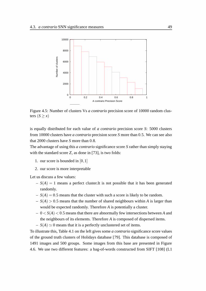
4.3. a contrario SNN significance measures 49
0
2000
4000
6000
8000
10000
0 0.2 0.4 0.6 0.8 1
Num
ber
of c
lust
ers
A contrario Precision Score
Figure 4.5: Number of clusters Vs a contrario precision score of 10000 random clus-ters (S ≥ x)
is equally distributed for each value of a contrario precision score S: 5000 clusters
from 10000 clusters have a contrario precision score S more than 0.5. We can see also
that 2000 clusters have S more than 0.8.
The advantage of using this a contrario significance score S rather than simply staying
with the standard score Z, as done in [73], is two folds:
1. our score is bounded in [0,1]
2. our score is more interpretable
Let us discuss a few values:
– S(A) = 1 means a perfect cluster.It is not possible that it has been generated
randomly.
– S(A) = 0.5 means that the cluster with such a score is likely to be random.
– S(A)> 0.5 means that the number of shared neighbours within A is larger than
would be expected randomly. Therefore A is potentially a cluster.
– 0 < S(A)< 0.5 means that there are abnormally few intersections between A and
the neighbours of its elements. Therefore A is composed of dispersed items.
– S(A)� 0 means that it is a perfectly unclustered set of items.
To illustrate this, Table 4.1 on the left gives some a contrario significance score values
of the ground truth clusters of Holidays database [79]. This database is composed of
1491 images and 500 groups. Some images from this base are presented in Figure
4.6. We use two different features: a bag-of-words constructed from SIFT [108] (L1

50 Chapter 4. Revisiting shared nearest neighbours clustering
distance), and a HSV Histogram [49].
On the right of the same Table 4.1, we illustrate the result for 500 random clusters
built from the 1491 images with a random size for each cluster.
The a contrario score somehow measures the difficulty to cluster a dataset. If, on
the true clusters, the a contrario score for HSV histogram is on average equal to 0.86,
it means that one cannot expect results better than this in a clustering result using the
same feature. So that, 14 of discovered clusters might be random ones. At the same
time, the results can not be worse on average than those of the random clusters using
the same feature (0.55).
Figure 4.6: Some images from Holidays database [79]
We can conclude that for those clusters and for this experiment, the HSV feature
is more structuring than the Bag of words feature.
Ground truth clusters Min Max Avg
Bow 0.55 1 0.71HSV Histogramme 0.67 1 0.86976
Random clusters Min Max Avg
Bow 0.51 0.6 0.56HSV Histogramme 0.53 0.57 0.55
Table 4.1: Holidays Database’s a contrario significance scores of the ground truthclusters (left) and of random clusters (right) by using bag-of words and HSV histogramfeatures.
Out of curiosity, we do the same experiment with another database: Corel1000

4.3. a contrario SNN significance measures 51
database [169]. The database contains 10 image classes with 100 images each. The
classes are: Africa, beach, buildings, buses, dinosaurs, flowers, elephants, horses, food
and mountains. This database was used in various scientific articles in the past for
content-based image retrieval systems. For this experiment, we use the HSV histogram
and the local feature SIFT. We present the a contrario score in Table 4.2.
For the ground truth clusters, the average of the a contrario score is equal to 0.98,
which means that, by using HSV histogram, this database is easier to cluster than the
Holidays database which is coherent with the fact that this dataset is known to be
“easy” for CBIR (Content-Based Image Retrieval) methods . Note that, by demon-
strating these two experiments, we do not claim in any way to say that HSV histogram
is better than Bow or SIFT. We rather want to show that having a target database and
a set of features, by means of computing the a contrario scores, we can select the
more structuring feature and having an idea about the difficulty of the database to be
clustered using the selected features.
Ground truth clusters Min Max Avg
Sift 0.81 1 0.78HSV Histogram 0.96 1 0.98
Random Clusters Min Max Avg
Sift 0.56 0.84 0.66HSV Histogram 0.53 0.79 0.68
Table 4.2: Corel1000 Database’s a contrario significance scores of the ground truthclusters (left) and of random clusters (right) by using SIFT and HSV histogram fea-tures.
4.3.3 Partial contributions to a set
Now that we have a normalised measure S(A) to qualify any set A, how would this
measure behave if a new element xi joins A? An item xi can have a greater contribution
to improve the quality of a cluster. Two cases are possible:
– if (S(A∪ xi)−S(A)> 0) then the contribution of the item xi increases the intra-
significance measure of the cluster, this means that this item is relevant to the
cluster and should be added to it. We call this Cluster reshaping.
– if (S(A∪ xi)− S(A) < 0) then the item is not relevant to the cluster. It has not
improved the quality of the cluster A.
However, recomputing the whole score S(A) for any new item xi would be inefficient
in a clustering framework. Fortunately S(A∪ xi) can be computed more efficiently
from S(A). We first show it with the intra-significance measure and the other measures

52 Chapter 4. Revisiting shared nearest neighbours clustering
as Z(A) and S(A) will be calculated as seen in Section 4.3.2.
I(A∪ xi)− I(A) =1
|A+1| ∑x∈(A∪xi)
|(A∪ xi)∩F|A+1|(x)|
− 1|A| ∑
x∈A
|A∩F|A|(x)|
=1
|A+1| [∑x∈A
|A∪ xi)∩F|A+1|(x)|
+|(A∪ xi)∩F|A+1|(xi)|]− 1|A| ∑
x∈A
|A∩F|A|(x)|
=1
|A+1| [∑x∈A
|(A∪ xi)∩F|A+1|(x)|
+|(A∪ xi)∩F|A+1|(xi)|]− 1|A| ∑
x∈A
|A∩F|A|(x)|
=1
|A+1| [∑x∈A
|A∩F|A|(x)|
+ ∑x∈A
|(A∪ xi)∩nn|A+1|(x)|
+|(A∪ xi)∩F|A+1|(xi)|]− 1|A| ∑
x∈A
|A∩F|A|(x)|
= [1
|A+1| −1|A| ] ∑x∈A
|A∩F|A|(x)|
+1
|A+1| [∑x∈A
|(A∪ xi)∩nn|A+1|(x)|
+|(A∪ xi)∩F|A+1|(xi)|] (4.14)
If we denote:
I1(A) = [1
|A+1| −1|A| ] ∑x∈A
(A∩F|A|(x)) (4.15)
and
I2(A,xi) =1
|A+1| [∑x∈A
((A∪ xi)∩nn|A+1|(x))
+((A∪ xi)∩F|A+1|(xi))] (4.16)
Then, the difference of intra-significance scores will be expressed as:
I(A∪ xi)− I(A) = I1(A)+ I2(A,xi) (4.17)

4.4. An efficient algorithm for building the shared-neighbours matrix 53
We do not recalculate all terms when adding a new item xi. The term I1(A) has al-
ready been calculated earlier and it only remains to calculate the second term I2(A)
which is very easy and fast to calculate. Thanks to this development, we avoid a time-
consuming computation.
4.3.4 Optimal neighbourhood
As we will see later, selecting the optimal neighbourhood of an item is an im-
portant step in our clustering algorithm. It can be done by running through all the
k-nearest neighbours from 1 to K and selecting the optimal rank kopt that maximizes
the a contrario score of the neighbourhood:
kopt(x) = argmaxk
S(Fk(x)) (4.18)
By this, we select only relevant neighbours among the k-NN list and we make our
method robust against noisy neighbours.
4.4 An efficient algorithm for building the shared-neighbours matrix
During the computation of the intra-significance measure, the most costly part
is calculating the number of shared neighbours between pairs of items for every
k = [1..K] to select the best neighbourhood. Therefore, we need an efficient way to
compute and to save the shared neighbours matrix (SNN Matrix) for any k.
The naive way would be to compute the intersection of K-NN of the entire set for
every k = [1..K]. This approach is time consuming and cannot be applied for most
applications due to its high complexity.
We propose a new factorisation algorithm to accelerate the calculation of shared neigh-
bours based on the same optimisation of the cluster reshaping computing as seen in the
previous section. As nnp(x) is the p-th nearest neighbour of an item x and Fk(x) is the
set of the k-nearest neighbours of x, we can define the intra-significance measure of a

54 Chapter 4. Revisiting shared nearest neighbours clustering
neighbourhood Fk(xi) of an item xi as:
I(Fk(x)) =1k ∑
x j∈Fk(x)
|Fk(x)∩Fk(x j)|
=1k[ ∑x j∈Fk−1(x)
|Fk−1(x)∩Fk−1(x j)|
+ ∑x j∈Fk−1(x)
|nnk(x j)∩nnk(x)|
+|Fk(x)∩Fk(nnk(x))|]=
1k[I(Fk−1(x))
+ ∑x j∈Fk−1(x)
|nnk(x j)∩nnk(x)|
+|Fk(x)∩Fk(nnk(x))|] (4.19)
Computing I(Fk(x)) for k = [1..K] is very time consuming, and the key idea of our
algorithm is to compute it recursively. We remark here that in Equation 4.19 that the
intra-significance measure of a neighbourhood Fk(x) of size k can be computed from
the previous intra-significance measure of the neighbourhood of x of size |k− 1| and
it only remains to compute the rest, which is very simple.
The final shared neighbours algorithm can be summarized in:
Input:the K-nearest neighbours matrix of size (N ×K).
Init: T = Zeros(N), I = zeros(N,K).
Output: I(Fk(x))
Algorithm 1 Fast shared neighbours of a variable neighbourhood from k = 1toK
for x = 1 to N dofor k = 1 to K do
for p = 1 to k doT (nnp(nnk(x)))+ = 1
end forfor p = 1 to k−1 do
T (nnp(nnk(x)))+ = 1end forfor q = 1 to k do
I(Fk(x))+ = T (nnq(x))end for
end forend for

4.5. Clustering framework 55
4.5 Clustering framework
4.5.1 Possible scenarios
The main goal of clustering is to identify distinct groups in a dataset. However, in
some applications, user wants to have the control in some aspects of groups. The num-
ber of distinct groups Nc in the data is a parameter that the user in some cases want to
fix as a prior. For most applications, this parameter is unknown, the clustering method
has to determine by itself the number of clusters by several strategies. Our proposed
clustering method is able to work in both cases.
Resulting clusters can present some intersection between them. Some clustering meth-
ods [183] of the state-of-the-art allow the overlap between clusters (soft clustering)
but others like [88] require elements to belong to a single cluster (hard clustering).
The maximum allowed overlap between two clusters is fixed by a parameter θOverlap.
Typically clusters sharing more than θOverlap elements, are considered redundant and
have to be merged efficiently.
In some cases, the quality of resulting clusters is limited to a minimum allowed thresh-
old θQuality. Clusters having less than θQuality are not accepted in the final list of clus-
ters. In our clustering method, the user can set this parameter θQuality of minimum a
contrario score of a cluster from the beginning. If this parameter has no importance
for the user, θQuality will be equal to 0.
In summary, we dispose of 3 optional parameters (Nc, θOverlap and θQuality) that lead
to different scenarios of clustering. Thanks to the a contrario score, the rate of quality
allowed is rather interpretable which facilitates the task of the user to fix it. The impact
of these parameters and their impact on the clustering result will be described in the
next Section.
4.5.2 Clustering method
Now that we have defined our new shared neighbours significance measures based
on the a contrario approach, we can describe our clustering. The goal is to find the
optimal clusters that maximize the a contrario scores.
This combinatorial problem cannot be solved exactly. In practice, we use a greedy
solution to reduce the number of solution by first considering each item as the center
of a candidate cluster. The following steps depend on the scenario that the user selects.
Our clustering algorithm is based on two main steps, candidate cluster construction
and final clusters selection. The first step is shared by the 3 scenarios and only the

56 Chapter 4. Revisiting shared nearest neighbours clustering
second step depends on which parameter is fixed or not.
Our proposed shared neighbours clustering is as follows:
– Candidate cluster construction: Each item x ∈ X is considered as a candidate
cluster center and an optimal candidate cluster C(x) needs to be computed for it.
We first compute an optimal neighbourhood Fkopt (x) by varying the neighbour-
hood size k from 1 to K and selecting the neighbourhood size that maximizes
our new a contrario score S (Eq.4.13):
kopt(x) = argmaxk
S(Fk(x))
Among the K neighbours of the item x, we finally keep the candidate cluster
Copt(x) which has the maximum S score:
Copt(x) = Fkopt (x)
We obtain N candidate clusters of different qualities.
– Final clusters selection: After the candidate cluster selection, we obtain some
potentially relevant clusters for each item but many of these clusters are still very
similar because close items might generate approximately the same candidate
cluster. Therefore, redundant clusters have to be eliminated and only different
seeds have to be selected.
For this step, we use a simple heuristic based on the overlap between candidate
clusters. The parameter θOverlap is generally used for this step. For that, first,
we sort all candidate clusters in decreasing order of their a contrario score and
then iterate on them. If an encountered cluster has an overlap (on percentage)
less than θOverlap with at least one of the previously retained clusters, it is added
to the final list of clusters.
If not, the encountered cluster is considered as similar to the retained cluster and
has to be used to reshape the retained cluster. For this: the contribution of all
items of both clusters to the retained cluster is computed (see Section4.3.3) and
sorted in decreasing order. The final retained cluster will be built from items that
increase the quality of the original retained cluster. This reshaping step is useful
because some relevant items from the original retained cluster may be greater
than others. It replaces poor associated items by other more strongly associated
items in order to yield a new improved retained cluster.

4.6. Experiments 57
If the parameter θOverlap is equal to zero, then a cluster is retained only if it
doesn’t share any item with the other retained clusters. Similar clusters are af-
fected to these different retained clusters and used to reshaping them. Note that,
in this case, an item is only assigned to one cluster.
In addition, for each retained cluster, we have its a contrario score in [0,1]. If the
user had limited the minimum allowed a contrario score to θQuality, all clusters
having less than θQuality will be eliminated from this list of final clusters.
In the case of knowing the number of clusters NC in advance, when iterating on
cluster to retain different clusters, we stop when achieving the target number of
clusters. The rest of clusters are assigned to one of the NC clusters according to
their intersection of them. They are used to reshape the NC retained clusters.
Overall, we remark here that our clustering framework requires essentially to know the
parameter θOverlap to decide if two clusters are similar which can be fixed by default
or done by the user. It can be chosen in a natural way with no knowledge of the nature
of the data set or its distribution. The other parameters are optional and used only if
the user has prior knowledge.
4.6 Experiments
4.6.1 Evaluation metrics
As discussed in Chapter 2, the choice of an evaluation metric depends on the goal
of the clustering experiment. In some applications, we evaluate the ability of the clus-
tering algorithm to discover the true categories (in a data mining perspective) whereas
in other application, we evaluate the quality of the clusters produced.
The metrics used in the experiments are as follows:
– AvgPurity: To measure the quality of the clusters produced, we measure the
Average Purity of all returned clusters. The Purity of a cluster C is defined
according to [22] by
Purity(C) =1
|C |max |Ch |
where Ch are the sub clusters composed of all the items of C coming from the
same ground truth category. max | Ch | is thus the dominant category of the
cluster.
– F1 measure: To measure the ability of the clustering algorithm to retrieve the

58 Chapter 4. Revisiting shared nearest neighbours clustering
initial categories, we define the F1 measure by:
F1 = 2∗ PREC×RECPREC+REC
with
PREC =#ofdistinctclusters
#ofretrievedclusters
and
REC =#distinctclusters
#ofClasses
Two clusters are considered to be distinct if their dominant categories differ.
– AvgCM: we measure the overall effectiveness of the clustering with the average
cosine measure (AvgCM) of all returning clusters based on the usual precision
and recall measures. To assess the quality of the clustering, we treat every center
q of a cluster C as a query returning the cluster and we compare it to the unique
class G of the ground-truth to which it belongs. The Cosine Measure CM of a
cluster in terms of its center q is defined by :
CM(q) =√
Prec(q).Recall(q)
with
Prec(q) =| G∩C || G |
and
Recall(q) =| G∩C ||C |
– The Rand index or Rand measure is a measure of the similarity between two
data clusterings : the ground truth clusters that we denote as X and the resulting
clusters that we denote as Y . We define :
– a, the number of pairs of elements that are in the same set in X and in the
same set in Y
– b, the number of pairs of elements that are in different sets in X and in different
sets in Y
– c, the number of pairs of elements that are in the same set in X and in different
sets in Y
– d, the number of pairs of elements that are in different sets in X and in the
same set in Y
The Rand index, R, is:
R = (a+b)/(a+b+ c+d)

4.6. Experiments 59
The Rand index has a value between 0 and 1, with 0 indicating that the two data
clusters do not agree on any pair of points and 1 indicating that the data clusters
are exactly the same.
4.6.2 Synthetic oracles definitions
Using synthetic data allows us to study individual effects separately, whereas using
real data sets usually makes it more difficult to isolate the various influences. In Section
4.3.1, we introduced one synthetic oracle i.e the random oracles. Here, we already
introduce other synthetic oracles attempting to model real systems in a generic way
(independently from metrics):
Definition 5. Perfect oracle:
Given a dataset X composed of N items, we define a perfect oracle as a function
returning the true K relevant nearest neighbours for each item.
Definition 6. No-perfect oracle:
Given a dataset X composed of N items, we define a no-perfect oracle as a function
returning, for each item x, r% of the true K nearest neighbours and (1− r)% of K
are items selected uniformly at random from X. All of the perfect neighbours and the
random neighbours are mixed together.
We define also an alternative of the no-perfect oracle that we call the Best first
oracle and which we define as follows:
Definition 7. Best first oracle:
Given a dataset X composed of N items, we define a best first oracle as a function
returning, for each item x, r% of the true K nearest neighbours and (1− r)% of K are
items selected uniformly at random from X.
Unlike the no-perfect oracle, perfect neighbours are returned first, followed by the
random neighbours.
Definition 8. Unstable oracle:
Given a dataset X composed of N items, we define an unstable oracle as a function
returning random neighbours for the (1− t)% of items. For the other t% of items, it
returns the true K-nearest neighbours.
Definition 9. No-perfect and unstable oracle:
Given a dataset X composed of N items, we define a no-perfect and unstable oracle
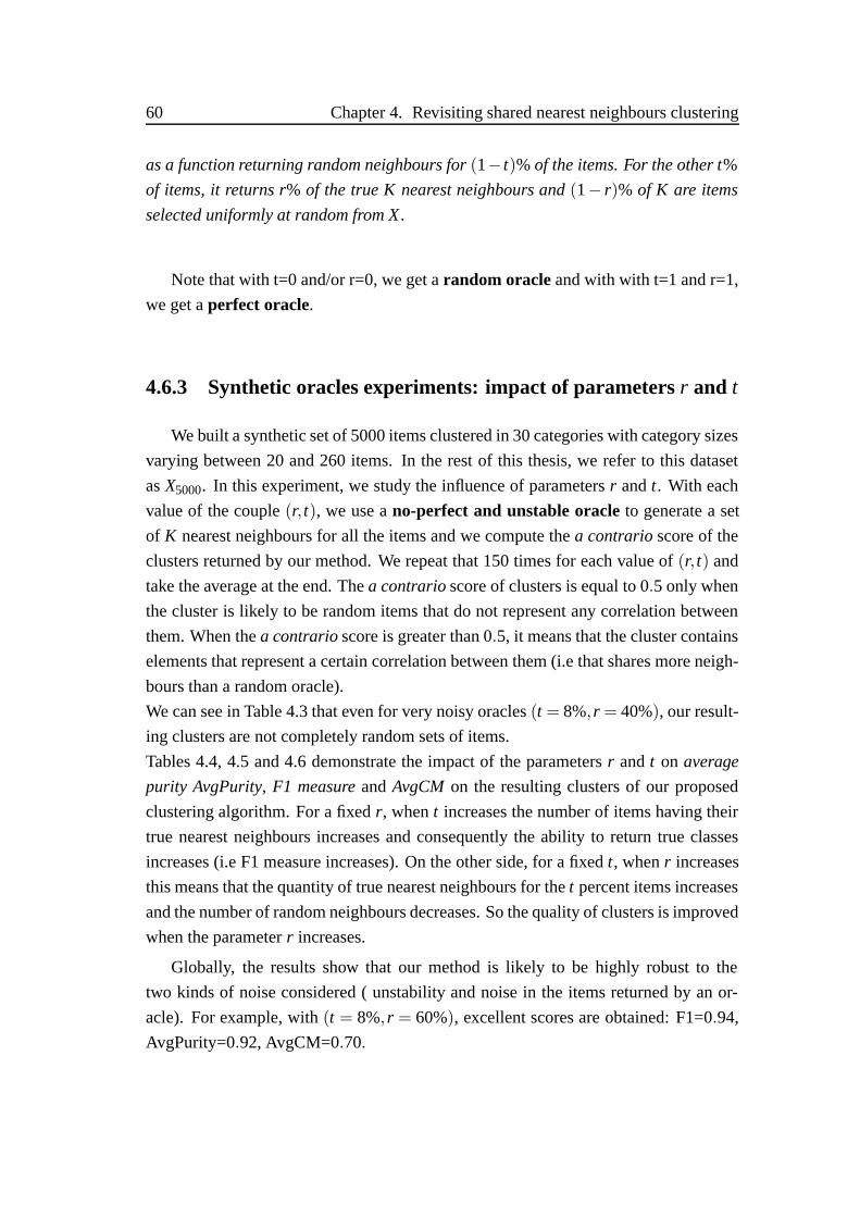
60 Chapter 4. Revisiting shared nearest neighbours clustering
as a function returning random neighbours for (1− t)% of the items. For the other t%
of items, it returns r% of the true K nearest neighbours and (1− r)% of K are items
selected uniformly at random from X.
Note that with t=0 and/or r=0, we get a random oracle and with with t=1 and r=1,
we get a perfect oracle.
4.6.3 Synthetic oracles experiments: impact of parameters r and t
We built a synthetic set of 5000 items clustered in 30 categories with category sizes
varying between 20 and 260 items. In the rest of this thesis, we refer to this dataset
as X5000. In this experiment, we study the influence of parameters r and t. With each
value of the couple (r, t), we use a no-perfect and unstable oracle to generate a set
of K nearest neighbours for all the items and we compute the a contrario score of the
clusters returned by our method. We repeat that 150 times for each value of (r, t) and
take the average at the end. The a contrario score of clusters is equal to 0.5 only when
the cluster is likely to be random items that do not represent any correlation between
them. When the a contrario score is greater than 0.5, it means that the cluster contains
elements that represent a certain correlation between them (i.e that shares more neigh-
bours than a random oracle).
We can see in Table 4.3 that even for very noisy oracles (t = 8%,r = 40%), our result-
ing clusters are not completely random sets of items.
Tables 4.4, 4.5 and 4.6 demonstrate the impact of the parameters r and t on average
purity AvgPurity, F1 measure and AvgCM on the resulting clusters of our proposed
clustering algorithm. For a fixed r, when t increases the number of items having their
true nearest neighbours increases and consequently the ability to return true classes
increases (i.e F1 measure increases). On the other side, for a fixed t, when r increases
this means that the quantity of true nearest neighbours for the t percent items increases
and the number of random neighbours decreases. So the quality of clusters is improved
when the parameter r increases.
Globally, the results show that our method is likely to be highly robust to the
two kinds of noise considered ( unstability and noise in the items returned by an or-
acle). For example, with (t = 8%,r = 60%), excellent scores are obtained: F1=0.94,
AvgPurity=0.92, AvgCM=0.70.

4.6. Experiments 61
,
t=8% t=10% t=12% t=20% t=40% t=60% t=80%
r=20% 0.5 0.5 0.5 0.5 0.5 0.5 0.51r=40% 0.7 0.79 0.81 0.87 0.88 0.92 0.97r=60% 0.92 0.95 0.96 0.97 0.98 0.99 1r=80% 0.97 1 1 1 1 1 1
r=100% 1 1 1 1 1 1 1
Table 4.3: Impact of r and t noise parameters on the a contrario score of the resultingclusters.
,
t=8% t=10% t=12% t=20% t=40% t=60% t=80%
r=20% 0.44 0.50 0.54 0.78 0.92 0.95 0.99r=40% 0.68 0.76 0.78 0.85 0.94 0.98 1r=60% 0.92 0.94 0.95 0.97 0.98 1 1r=80% 0.98 0.99 1 1 1 1 1
r=100% 1 1 1 1 1 1 1
Table 4.4: Impact of r and t noise parameters on the AvgPurity measure of the resultingclusters
,
t=8% t=10% t=12% t=20% t=40% t=60% t=80%
r=20% 0.42 0.44 0.48 0.49 0.52 0.56 0.60r=40% 0.74 0.79 0.8 0.86 0.87 0.91 0.95r=60% 0.94 0.95 0.96 0.97 0.97 0.98 0.99r=80% 0.98 1 1 1 1 1 1
r=100% 0.99 1 1 1 1 1 1
Table 4.5: Impact of r and t noise parameters on the F1 measure of the resulting clusters
,
t=8% t=10% t=12% t=20% t=40% t=60% t=80%
r=20% 0.07 0.09 0.11 0.21 0.37 0.41 0.42r=40% 0.30 0.40 0.42 0. 48 0.50 0.53 0.64r=60% 0.70 0.71 0.72 0.73 0.74 0.75 0.80r=80% 0.86 0.88 0.89 0.9 0.92 0.96 0.99
r=100% 0.99 0.99 1 1 1 1 1
Table 4.6: Impact of r and t noise parameters on the AvgCM measure of the resultingclusters

62 Chapter 4. Revisiting shared nearest neighbours clustering
4.6.4 Optimal radius for computing candidate clusters
To validate that our approach tends to select the optimal neighbourhood of any
candidate clusters, we use the same dataset X5000 from the previous experiment and
the best first oracle with parameters (r = 80%, t = 100%) to generate the K-nearest
neighbours. This means, that each item xi has as its neighbours r = 80% of the cluster
C(xi) to which it belongs and the rest is a set of items selected uniformly at random of
X5000 −C(xi). It is important to note that items from the r = 80% of the cluster C(xi)
are also selected randomly, so two items from the same cluster may not have the same
neighbours.
In the Candidate cluster construction step of our clustering framework, we obtain
for each item xi, the optimal neighbourhood size kopt (see Section 4.5) equal to the
r = 80% of the cluster to which xi belongs. This confirms that only relevant items are
selected when looking for the optimal neighbourhood size.
After this step, for each item , we obtain a candidate cluster containing only relevant
items from the cluster to which it belongs. By using the second step of our clustering
framework i.e. final clusters selection, we obtain at the end 30 different clusters that
represent all the categories of the ground truth and we eliminate redundant clusters.
4.6.5 Impact of the overlap parameter
The overlap parameter is the only parameter that the user has to fix in our algo-
rithm. To evaluate the impact of this parameter, we use the same dataset X5000 and
a no-perfect and unstable oracle to generate two lists of K nearest neighbours of
items. The first one is computed with (r = 40%, t = 8%) and the second one with
(r = 60%, t = 8%). We vary the parameter of overlap θOverlap when eliminating the
redundant clusters and we compute the F1 measure and the AvgCM of resulting final
clusters. Figure 4.7 shows how the F1 measure remains stable until a particular value
(40% for the square and triangle lines and 50% for dots and crosses lines). When the
θOverlap increases, we allow more overlap between clusters so the number of clusters
considered as different increases which decreases the F1 measure. In the case of a
small value of θOverlap, we select the most different clusters which represent the initial
classes. When the goal of a user is to have the more representative clusters of a dataset,
we recommend to choose a small value of θOverlap. We generally fix this parameter to
50% when no constraints are required.
On the other hand, we can see that the AvgCM measure is not very sensitive to the
overlap parameter because we use a greedy strategy to eliminate redundant clusters in
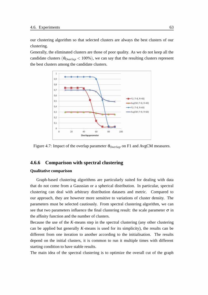
4.6. Experiments 63
our clustering algorithm so that selected clusters are always the best clusters of our
clustering.
Generally, the eliminated clusters are those of poor quality. As we do not keep all the
candidate clusters (θOverlap < 100%), we can say that the resulting clusters represent
the best clusters among the candidate clusters.
Figure 4.7: Impact of the overlap parameter θOverlap on F1 and AvgCM measures.
4.6.6 Comparison with spectral clustering
Qualitative comparison
Graph-based clustering algorithms are particularly suited for dealing with data
that do not come from a Gaussian or a spherical distribution. In particular, spectral
clustering can deal with arbitrary distribution datasets and metric. Compared to
our approach, they are however more sensitive to variations of cluster density. The
parameters must be selected cautiously. From spectral clustering algorithm, we can
see that two parameters influence the final clustering result: the scale parameter σ in
the affinity function and the number of clusters.
Because the use of the K-means step in the spectral clustering (any other clustering
can be applied but generally K-means is used for its simplicity), the results can be
different from one iteration to another according to the initialisation. The results
depend on the initial clusters, it is common to run it multiple times with different
starting condition to have stable results.
The main idea of the spectral clustering is to optimize the overall cut of the graph

64 Chapter 4. Revisiting shared nearest neighbours clustering
while in our proposed SNN method, we aim to select an optimal neighbourhood for
each item and to merge redundant clusters by simple heuristics.
In spectral clustering, the choice of the graph, as described in Section 2.4, influences
the results [111]. If a K-nearest neighbour graph is chosen, the parameter K is critical
and has to be fixed carefully: if K is very limited, some relevant neighbours are
disconnected, whereas if K is very large, outliers are connected to relevant neighbours.
In our proposed clustering method, note that thanks to the selection of the optimal
neighbourhood even if K is large, only relevant nearest neighbours that maximize the
quality of the neighbourhood are selected: outliers are ignored and not considered as
relevant neighbours even if the parameter K has allowed it to be connected to the item.
In the case of a limited K, thanks to the reshaping step, we recover the elements that
we missed.
Another difference with spectral clustering is that in our method, an item can belong
to different clusters, whereas spectral clustering is generally a hard clustering, because
ultimately K-means selects one cluster for each item.
Although some recent works [180, 21] propose methods to tune the scale parameter
and the number of clusters automatically, the results remain sensitive to the choice of
the method or the heuristic whereas in our method the number of clusters is produced
automatically and the only predefined overlap threshold can be determined without
any knowledge of the data to cluster.
A last difference with spectral clustering is the robustness of our method. If the source
that produce the K nearest neighbours of an item is noisy or contains some errors,
the spectral clustering will take the generated graph as it is and look for the optimal
cut, which obligatory lead to irrelevant results. In our case, thanks to the selection of
the optimal neighbourhood and the reshaping steps, irrelevant neighbours, even those
having a low rank by mistake, will not be considered as relevant because by including
them, they did not improve the quality of the cluster.
Quantitative comparison
To compare our proposed clustering method to spectral clustering algorithms, we
choose the two standard versions described in the state-of-the-art (see Section 2.4.1):
the normalized spectral clustering according to Shi and Malik [146] and the normalized
spectral clustering according to Ng, Jordan and Weiss [121].
For this, we use two common datasets: the Iris Plants Database [53] and the Wine

4.6. Experiments 65
dataset usually used in papers dealing with spectral clustering issues. Iris Dataset is
perhaps the best known database to be found in the pattern recognition literature. It
can be download on 1. The data set contains 3 classes of 50 instances each, where each
class refers to a type of iris plant. One class is linearly separable from the other 2;
the two others are not linearly separable from each other. The Number of Attributes is
equal to 4 numeric predictive attributes and the class:
– sepal length in cm
– sepal width in cm
– petal length in cm
– petal width in cm
– classes: Iris Setosa, Iris Versicolour, Iris Virginica
The scope of “Wine Data Set” is related to chemical analysis. The task consists
in regrouping 178 items from the same origin of wines in 3 classes. Created by [164]
and available on 2, this dataset is the results of a chemical analysis of wines grown
in the same region in Italy but derived from three different cultivators. The analysis
determined the quantities of 13 constituents found in each of the three types of wines.
All attributes are continuous:
– Alcohol
– Malic acid
– Ash
– Alcalinity of ash
– Magnesium
– Total phenols
– Flavanoids
– Nonflavanoid phenols
– Proanthocyanins
– Color intensity
– Hue
– OD280/OD315 of diluted wines
– Proline
The number of instances per class is respectively : 59, 71, 48. For all methods, the
Euclidean distance was used as a pairwise similarity measure. For tested spectral clus-
tering methods , the number of clusters is given as input whereas our method finds by
itself automatically the right number of clusters for the two data sets. We can say that
1. http://archive.ics.uci.edu/ml/datasets/Iris2. http://archive.ics.uci.edu/ml/datasets/Wine

66 Chapter 4. Revisiting shared nearest neighbours clustering
in this experimentation, the spectral clustering has more advantages than our method
from the start.
Concerning the scale parameter σ needed in the spectral clustering, we use the method
proposed by [146]. They gave a range of the scale parameter as:
σ = c× (max(dist)−min(dist)) (4.20)
with c ∈ [0.1,0.2].
For the overlap parameter of our proposed shared nearest neighbours clustering, we
fix it to 50% as discussed earlier in Section 4.5. We remember that this parameter is
the maximum overlap allowed between two clusters to be considered as two different
clusters. If the overlap exceeds 50%, the two clusters are considered as similar and
have to be grouped on a relevant single cluster by reshaping.
For the evaluation, we use two metrics : the Rand Index [140] and the Average Purity
(see Section 4.6.1). The results of the two datasets are reported in Tables 4.7and 4.8.
Note that as spectral clustering use K-means the results differ from an iteration to
another, we iterate 50 times and take the average.
Ng, Jordan and Weiss Shi and Malik Our SNN clustering
Rand index 0.87 0.75 0.83Avg Purity 0.9 0.8 0.87
Table 4.7: The Iris Plants Database clustering results
Ng, Jordan and Weiss Shi and Malik Our SNN clustering
Rand index 0.62 0.48 0.72Avg Purity 0.81 0.78 0.70
Table 4.8: The Wine Database clustering results
Through this experimentation, we want to show that the performances our SNN
clustering results do not differ greatly from those of the two spectral clustering meth-
ods tested here although that we did not give any a priori information to our clustering
(i.e the number of clusters). By keeping the overlap threshold to 50% which can be
kept for all experiments in this PhD. Our clustering method finds automatically the
right number of clusters and the results are very promising. For standard spectral
clustering that we tested, it was necessary to give the number of clusters as input, com-
puting the best value of the scale parameter for the affinity matrix and finally iterating

4.6. Experiments 67
several times to have stable results.
We then studied the impact of the neighbourhood size on our SNN clustering compared
to the spectral clustering of Ng, Jordan and Weiss. For this, we used the synthetic data
X5000 build from 5000 items clustered in 30 categories with different size between 20
and 260 items. We vary the value of the k nearest neighbours and we compute the
AvgPurity and the Rand Index. Results are reported in Figures 4.8 and 4.9.
For spectral clustering [121], we can denote that by increasing the neighbourhood size,
the average purity and the rand index values increase smoothly for the spectral cluster-
ing with the best tuning (the right number of clusters is done and we take the best scale
parameter). For k = 50, the used spectral algorithm diverges : items are disconnected
and the algorithm cannot find the 30 categories. This is why we had to begin with
K = 100 in the experiment.
This is not the case for our proposed clustering, which deals with a small neighbour-
hood (for k = 50,AvgPurity= 1 and RandIndex = 0,98). Thanks to the reshaping step
during the elimination of the redundant clusters, even with small neighbourhood, our
clustering adds relevant missing items to their relative clusters.
By this experiment, we can conclude that our SNN clustering is robust and less sen-
sitive to the neighbourhood size than the spectral clustering [121]. It also shows, that
our method is globally more robust to the kind of noises considered in this experiment
(unstability and noisy returned items).
Figure 4.8: Impact of the neighbourhood size on the AvgPurity and the Rand Indexvalues when using the spectral clustering [121]

68 Chapter 4. Revisiting shared nearest neighbours clustering
Figure 4.9: Impact of the neighbourhood size on the AvgPurity and the Rand Indexvalues when using our proposed SNN clustering
4.7 Conclusion
In this chapter, we revisited an existing shared neighbours methods in two points.
We first introduced a new SNN formalism based on the theory of a contrario decision.
This allows us to derive more reliable connectivity scores of candidate clusters and a
more intuitive interpretation of locally optimum neighbourhoods. We also proposed a
new factorization algorithm for speeding-up the intensive computation of the required
shared neighbours matrices. We compared our proposed method to a spectral cluster-
ing [121]. We showed that our method is globally more robust to the kind of noises
considered in the experiment (unstability and noisy returned items).
This chapter is the basis for the second and the third contributions of this work.

Chapter 5
Multi-source shared nearestneighbours clustering
5.1 The multi-source SN problem
The increasing availability of devices (laptops, smart phones, camera) has led to
an explosion in the amount of information that user must confront in order to use them
efficiently. We are often given unsupervised data originating from different sources.
For example, images have many properties (color, texture, etc) and meta-data (textual
annotation, EXIF, etc) which are quite different from one source of information to an-
other. The goal is to benefit from all available sources of information so as to be able
to have more meaningful information concerning the images. To harness the strengths
of that, multi-modality processing has become an attractive strategy.
It is known that processing data from a single irrelevant information source will con-
tribute to the creation of a bad result. Does the use of multiple data sources had more
chance to improve the result? How can we deal with sources when some of them are
characterized uncertain information ? We need an efficient combination of sources and
not just a trivial fusion. An effective combination is crucial.
In order to deal with uncertainty in the available data, we propose to determine a clus-
tering that is consistent not with all sources but with the optimal subset of sources.
For each cluster, we need to select relevant information sources and ignore irrelevant
ones. In this way, noise can be reduced by combining sources effectively and can over-
come the bad quality of sources by correcting the errors produced by each individual
source. Imagine that a search engine asks M decentralized servers to return the K first
responses to a user’s query and it merges the M lists to produce a final ranking of re-
sults. What happens if one or multiple servers return junk results ? Will the search

70 Chapter 5. Multi-source shared nearest neighbours clustering
engine find that one source of information returns results with no significance ? This
can be avoided if we merge not only the results of all available sources but we select
the optimal subset of sources ? We will try to answer these questions in this Chapter.
A second problem is how to group observations that belong to different physical spaces
with different dimensionalities, e.g., how to group visual data with textual data ? To do
this, shared neighbours clustering seems appropriate because even in heterogeneous
contexts in which underlying features and similarity values do not have a straight-
forward unique interpretation, two items having a high proportion of neighbours in
common can be assigned to the same group. Two items are considered to be well-
associated not by virtue of their pairwise similarity value, but by the degree to which
their neighbourhoods resemble one another.
Shared nearest neighbours (SNN) methods thus appear to be ideally suited to multi-
modal clustering. Because they are based on conexity information only and not on
densities or metrics in some feature spaces, heterogeneous information sources can be
embedded identically and easily compared or fused. SNN method, as stated before,
are able to overcome several shortcomings of traditional clustering approaches: they
do not suffer from the curse of dimensionality, they are robust to noisy data, they do not
need to initially fix the number of clusters, and, last but not least, they do not require
any explicit knowledge of the nature or representation of the data. These properties
make them widely generic for multimedia mining or structuring purposes, whatever
the targeted objects and the required similarity measures.
In this chapter, we introduce, a new generic multi-source SNN framework including
new multi-source measures for arbitrary object sets and information sources. The main
originality of our approach is that we introduce an information source selection step
in the computation of these measures thanks to an a contrario standardization of the
sum of the individual SNN scores. In addition to a usual conexity score, any arbitrary
object set is thus associated with its own optimal subset of modalities maximizing the
multi-source a contrario score. All resulting clusters do not necessarily have the same
selected sources in contrast to other previous work.
5.2 A contrario multi-source SNN significance mea-sures
To generalize a shared neighbours clustering to a multi-source environment, several
issues have to be solved. Whereas in a single source model, each item of the dataset

5.2. A contrario multi-source SNN significance measures 71
X = {xi}i=[1..N] to be clustered is associated with a single nearest neighbours list, in
the multi-source environment, each item is associated with m nearest neighbours lists
where m corresponds to the number of sources. In the following, we denote as O the set
of available information sources and m = |O| the number of sources. Any information
source o ∈ O is defined only by its nearest neighbours response function FK(x,o):
FK(x,o) = {nnok}k∈[1,K]
where x represents any item of the whole dataset X to be clustered and nnok ∈ X the
k-th nearest neighbour of the item x according to the source o.
5.2.1 Raw multi-source SNN significance measures
We first generalise the intra-significance measure (Equation 4.2) seen in Chapter
4.3 to the multi-source case, by measuring the expectation of the inter-set correlation
between a set A and the nearest neighbours set of an item x selected uniformly at
random from A according to an information source o selected uniformly at random
from O.
As a primary multi-source intra-set significance measure for any set A ⊂ X , we have:
Definition: Multi-source intra-significance measure
I(A,O) =1
|A||O| ∑o∈O
∑x∈A
(A∩F|A|(x,o))
=1
|A||O| ∑o∈O
∑x∈A
IA(x,o) (5.1)
Comparing the multi-source intra-set significance measure of sets of different sizes
and different amounts of information sources is biased. It is not only regarding the
size as in the mono-source case (see the section 4.2) but also concerning the number
of sources. How can we normalize this measure to be able to compare and sort the sets
of items regardless of their size and their selected sources ?
5.2.2 A contrario normalization
As in the mono-source case, we propose to remove the bias of the raw measure
by the a contrario principle. Let us call H ′ the null hypothesis that all sources are
i.i.d and uniformly distributed, i.e. each source returns nearest neighbours selected
uniformly at random from X (all sources are independent random Oracles). Under
the hypothesis H ′, the multi-source intra-significance measure is normally distributed

72 Chapter 5. Multi-source shared nearest neighbours clustering
and the IA(x,o) is a hypergeometrically distributed random variable with expectation :
E[IA(x,o)] =|A|2N
(5.2)
and variance :
Var[IA(x,o)] =|A|2(|N|− |A|)2
N2(N −1)(5.3)
by using the central limit theorem, we can conclude that I(A,O) is assumed to follow
a normal distribution N (μA,σ 2A) with:
μA = E[I(A,O] = E[IA(x,o)]
=|A|2N
(5.4)
Because of the independence of IA(x,o) variables, we obtain for the variance:
σ 2A = Var[I(A,O)] =
Var[IA(x,o)]|O||A|
=|A|(N −|A|)2
|O|N2(N −1)(5.5)
Note that in Equation 5.5, for a fixed size set |A|, the more sources we have, the smaller
the variance is. I(A,O) can therefore be standardized to a multi-source standard normal
distribution Z(A,O) with parameters N (0,1) under the hypothesis H ′ as follows:
Z(A,O) =I(A,O)−E[I(A,O)]√
Var[I(A,O)]
=√|O| |A|(N −|A|)2
N2(N −1)(I(A,O)−E[I(A,O)])
=√|O|[ I(A,O)−E[I(A)]√
Var[I(A)]]
=√|O|[
1|O| ∑|O|
o=1 I(A,o)−E[I(A)]√Var[I(A)]
] (5.6)
As we have now a multi-source standard significance measure Z under the null hy-
pothesis H ′, we can estimate the precision score a contrario to H ′ as follows:
PZ(A,O)(z) =
∫ z
−∞
1√2Π
e−t22 dt
= 1−φ(z) (5.7)

5.3. Cluster-centric selection of optimal sources 73
where φ()is the cumulative distribution function of the standard normal distribution
that describes probabilities for a random variable to fall within the interval ]−∞,z].
PZ(A,O)(z) is the probability that the multi-source standard significance measure
Z(A,O) does not exceed a threshold z under the null hypothesis H ′ in the multi-
source case.
So that , P f a(z) = 1−PZ(A,O)(z) is the likelihood that A is not a false alarm (i.e the
likelihood that the subset A was not generated by a subset of random oracles).
P f a(z) can also be expressed in terms of the error function erf as follows:
P f a(z) =12− 1
2erf(
z√2) (5.8)
Having the probability of a false alarm under the null hypothesis, we can now deter-
mine our multi-source a contrario significance score as the complement of the P f a :
Definition Multi-source a contrario significance score:
S(A,O) = 1−P f a(Z(A,O))
= 1−φ(Z(A,0))
=12+
12
erf(Z(A,O)√
2) (5.9)
5.3 Cluster-centric selection of optimal sources
Now that we have a precision score that is unbiased relative to the number of infor-
mation sources, we can describe our approach to select the optimal subset of sources
of any input set A. If we denote as θ ⊆ O an arbitrary subset of sources, then we are

74 Chapter 5. Multi-source shared nearest neighbours clustering
searching for the optimal subset θopt(A)⊆ O maximizing S(A,θ):
θopt(A) = argmaxθ⊆O
(S(A,θ))
= argmaxθ⊆O
(12+
12
erf(Z(A,θ)√
2
)= argmax
θ⊆OZ(A,θ)
= argmaxθ⊆O
[I(A,θ)−E[I(A,θ)]√
Var[I(A,θ)]]
= argmaxθ⊆O
√|θ |[ 1
|θ | ∑o∈θ
I(A,o)]
= argmaxθ⊆O
1√|θ | ∑o∈θ
I(A,o)
= argmaxi<|O|
argmaxθ⊆O\|θ |=i
1√|θ | ∑o∈θ
I(A,o)
= argmaxi
1√iargmaxθ\|θ |=i
∑o∈θ
I(A,o)
= argmaxi
1√i∑
o∈θi
I(A,o) (5.10)
In this way, we are not only seeking the best number of sources i but also selecting the
best combination of sources of size i . θi is the optimal combination of sources of size
i.
What seemed at first glance to be a combinatorial problem can indeed be solved ex-
tremely easily by pre-sorting single-sources intra-significances in decreasing order and
finding the optimal number of top sources θopt .
Our final selected-source intra-significance measure of any arbitrary set A is finally
given by:
Iopt(A,θopt(A)) =1√|θopt| ∑
oi∈θopt(A)
I(A,oi) (5.11)
This indicates that if the intra-significance measures for A are available with respect
to individual oracles and have been presorted from highest to lowest, then the most
significant sub collection of oracles describing A, over a desired range of sub collection
sizes, can be determined in linear time.
In the same way, the optimal multi-source a contrario score S can be computed by
combining the individual a contrario scores according to the optimal subset of sources

5.4. Clustering framework 75
θopt :
S(A,θ) = S(A,θopt(A)) (5.12)
The goal of selecting the optimal subset of sources is to avoid outlier sources in O. Un-
like methods that use all available sources to compute the significance of a set whatever
the quality of the information sources, we only select sources that maximize the quality
of the set A and ignore the rest.
5.4 Clustering framework
Now that we have defined our new multi-source shared nearest neighbours
significance measures we can describe our multi-source clustering procedure. It is
based on three main steps, unlike the mono-source case which was based in only two
steps. The three steps are: candidate cluster construction, candidate cluster reshaping
and final clusters selection.
– Candidate cluster construction: Each item x ∈ X is considered as a candidate
cluster center and an optimal candidate cluster C(x) needs to be computed
for it. For each source oi ∈ O , every item has a list of K-NN. For that, we
have to select the optimal neighbourhood in each K-NN that maximizes our
multi-source a contrario score S (Equation 5.9).
Note that an optimal source selection is performed for each iteration on the
neighbourhood size k and the selected subset θopt(Fk(x,oi)) of sources may
differ from one value of k to another.
The optimal neighbourhood koi(x,O) for the item x according to the source
oi ∈ O is defined by:
koi(x,O) = argmaxk
S(Fk(x,oi),O)
= argmaxk
S(Fk(x,oi),θopt(Fk(x,oi))) (5.13)
Unlike the mono-source case, where each item is represented by a single neigh-
bourhood, in the multi-source case, for each source oi ∈O, we obtain the optimal
neighbourhood. Among the m list of optimal neighbourhoods koi(x,O) of the
item x according the each single source oi, we finally keep as a candidate cluster

76 Chapter 5. Multi-source shared nearest neighbours clustering
Copt(x) the neighbourhood of the source o j that has the maximum multi-source
a contrario score S:
Copt(x) = Fk(x,θopt(Fk(x,o j))
Each candidate cluster is defined by its own optimal subset of sources that are
the most relevant for it.
– candidate cluster reshaping: After selecting the single optimal neighbour-
hood with its own optimal subset of sources, some neighbours provided by each
source of the selected sources may be more relevant to Copt(x). The candidate
cluster Copt(x) is the best set of K-NN provided by a source o j because it has the
maximum multi-source a contrario score. By selecting just one neighbourhood,
some other relevant neighbours provided from the other sources (selected in the
optimal subset of sources) may be missing. The contribution of some relevant
items from the other neighbours of x can improve the quality of Copt(x).
For this reason, each candidate cluster Copt(x) has to be reshaped by adding only
the strongly associated items provided from the remaining optimized neighbour-
hoods, those from sources included in the selected subset θopt(x,o j) of sources.
We denote these items as K ′-NN. For each item y in K′-NN, we compute its own
contribution c(y,Copt(x)\θopt(x,o j)) to the candidate cluster Copt(x) centred on
x and provided by the source o j. This contribution is based on the selected opti-
mal subset of sources θopt(x,o j) as described in the following equation:
c(y,Copt(x)\θopt(x,o j)) =1
|Copt(x)||θopt(x,o j)|∑
o∈θopt(x,o j)
|(Copt(x)∩F|Copt(x)|(y,o)|
(5.14)
We sort in decreasing order the contribution of each y in K ′-NN to C(x) and
we select those who decrease the quality of the candidate cluster Copt(x) i.e
that maximize the final multi-source precision score S(Copt(x,θopt)) as seen in
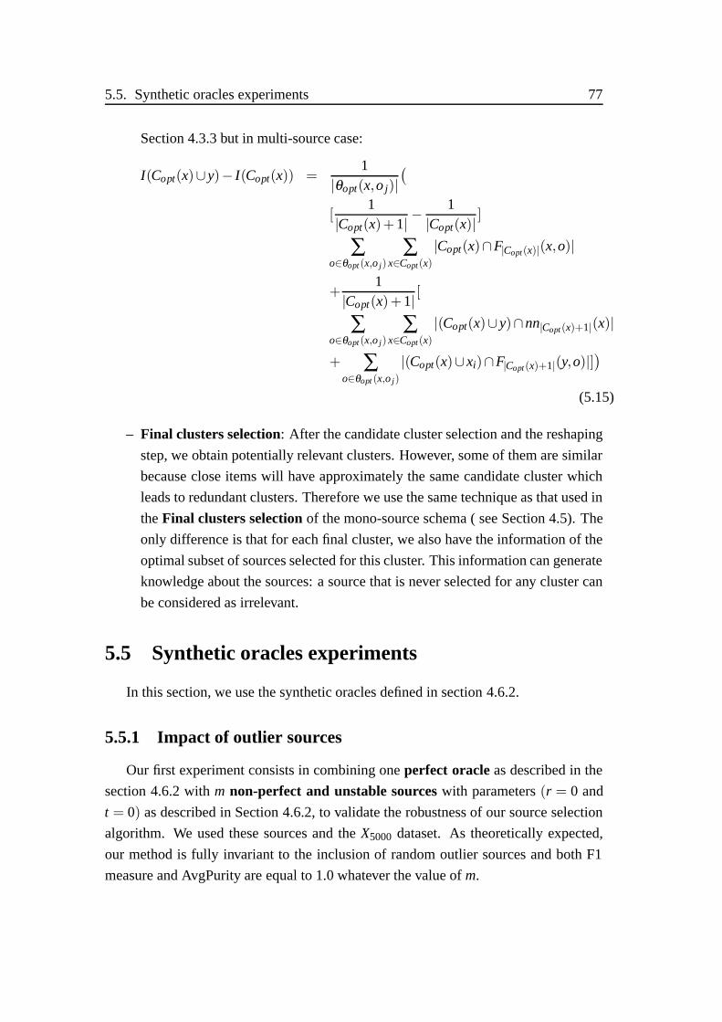
5.5. Synthetic oracles experiments 77
Section 4.3.3 but in multi-source case:
I(Copt(x)∪ y)− I(Copt(x)) =1
|θopt(x,o j)|(
[1
|Copt(x)+1| −1
|Copt(x)| ]
∑o∈θopt (x,o j)
∑x∈Copt(x)
|Copt(x)∩F|Copt(x)|(x,o)|
+1
|Copt(x)+1| [
∑o∈θopt (x,o j)
∑x∈Copt(x)
|(Copt(x)∪ y)∩nn|Copt(x)+1|(x)|
+ ∑o∈θopt (x,o j)
|(Copt(x)∪ xi)∩F|Copt(x)+1|(y,o)|])
(5.15)
– Final clusters selection: After the candidate cluster selection and the reshaping
step, we obtain potentially relevant clusters. However, some of them are similar
because close items will have approximately the same candidate cluster which
leads to redundant clusters. Therefore we use the same technique as that used in
the Final clusters selection of the mono-source schema ( see Section 4.5). The
only difference is that for each final cluster, we also have the information of the
optimal subset of sources selected for this cluster. This information can generate
knowledge about the sources: a source that is never selected for any cluster can
be considered as irrelevant.
5.5 Synthetic oracles experiments
In this section, we use the synthetic oracles defined in section 4.6.2.
5.5.1 Impact of outlier sources
Our first experiment consists in combining one perfect oracle as described in the
section 4.6.2 with m non-perfect and unstable sources with parameters (r = 0 and
t = 0) as described in Section 4.6.2, to validate the robustness of our source selection
algorithm. We used these sources and the X5000 dataset. As theoretically expected,
our method is fully invariant to the inclusion of random outlier sources and both F1
measure and AvgPurity are equal to 1.0 whatever the value of m.

78 Chapter 5. Multi-source shared nearest neighbours clustering
5.5.2 Impact of source precision and stability parameters
Our second experiment is to study the influence of parameters t and r when com-
bining several non-perfect and unstable information sources. For this experiment,
we used m = 4 oracles and we varied the value of r and t. We use the same dataset
X5000 described in 4.6.3 but the difference of this experiment relative to the experiment
done in 4.6.3 is that here we are evaluating the a contrario score, the F1 measure,
the AvgPurity and the AvgCM of our resulting clusters in a multi-source case. By
this experiment, we aim to show the interest of using multiple sources even if they
are non-perfect and unstable. The results of the F1 measure and the average cosine
measure (AvgCM) in multi-sources case are reported in Tables 5.2 and 5.3, the a
contrario scores of clusters are reported in 5.1.
Note that thanks to the oracle selection and the reshaping steps, all produced clusters
present AvgPurity = 1, this means that only relevant items are kept in clusters.
The a contrario scores even with low quality of K-nearest neighbours of cluster’s
items (r = 20%, t = 8%) still relevant clusters (a contrario score=0.97) which means
that the clusters are far from random sets. Compared to the mono-source case (Table
4.3), the score has almost doubled.
Tables 5.2 and 5.3 show that our method is robust to both kinds of noise, i.e im-
precision and unstability. Compared to the results showed in the mono-source case
described in the section 4.6.3, we can see how results are improved by combining
4 non-perfect and unstable oracles. For example, even with low quality of nearest
neighbours (r = 40% and t = 8%), the F1 measure increases from 0.74 in the
mono-source case to 0.99 in the multi-source case. For the same parameters, the
AvgCM increases from 0.30 to 0.62 by using 4 sources. That means that our method is
able to compensate the weak quality of very noisy independent sources by combining
them effectively even with only 4 sources.
Note that all these results could be more improved if we had used more sources as
done in the next section.
5.5.3 Impact of the number of sources
We study the impact of the number of sources on the effectiveness of our method.
For this experiment we fixed r and t and we varied the number of unstable and
no-perfect oracles from 1 to 14. We do that by using a couple of parameters
(r = 40%, t = 10%). The results are provided in Figure 5.1. It shows that increas-
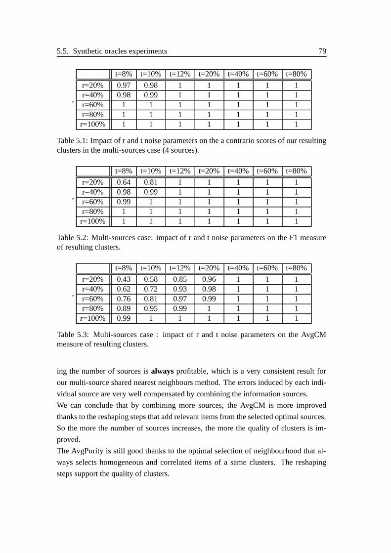
5.5. Synthetic oracles experiments 79
,
t=8% t=10% t=12% t=20% t=40% t=60% t=80%
r=20% 0.97 0.98 1 1 1 1 1r=40% 0.98 0.99 1 1 1 1 1r=60% 1 1 1 1 1 1 1r=80% 1 1 1 1 1 1 1
r=100% 1 1 1 1 1 1 1
Table 5.1: Impact of r and t noise parameters on the a contrario scores of our resultingclusters in the multi-sources case (4 sources).
,
t=8% t=10% t=12% t=20% t=40% t=60% t=80%
r=20% 0.64 0.81 1 1 1 1 1r=40% 0.98 0.99 1 1 1 1 1r=60% 0.99 1 1 1 1 1 1r=80% 1 1 1 1 1 1 1
r=100% 1 1 1 1 1 1 1
Table 5.2: Multi-sources case: impact of r and t noise parameters on the F1 measureof resulting clusters.
,
t=8% t=10% t=12% t=20% t=40% t=60% t=80%
r=20% 0.43 0.58 0.85 0.96 1 1 1r=40% 0.62 0.72 0.93 0.98 1 1 1r=60% 0.76 0.81 0.97 0.99 1 1 1r=80% 0.89 0.95 0.99 1 1 1 1
r=100% 0.99 1 1 1 1 1 1
Table 5.3: Multi-sources case : impact of r and t noise parameters on the AvgCMmeasure of resulting clusters.
ing the number of sources is always profitable, which is a very consistent result for
our multi-source shared nearest neighbours method. The errors induced by each indi-
vidual source are very well compensated by combining the information sources.
We can conclude that by combining more sources, the AvgCM is more improved
thanks to the reshaping steps that add relevant items from the selected optimal sources.
So the more the number of sources increases, the more the quality of clusters is im-
proved.
The AvgPurity is still good thanks to the optimal selection of neighbourhood that al-
ways selects homogeneous and correlated items of a same clusters. The reshaping
steps support the quality of clusters.

80 Chapter 5. Multi-source shared nearest neighbours clustering
Finally, the F1 measure is still also good thanks to the correlated steps: the elimination
of redundant clusters and the use of poor clusters to reshape relevant ones.
Figure 5.1: Impact of the information sources number on AvgPurity, F1 measure andthe AvgCM.
5.5.4 Computational time analysis
Finally, we study the time execution of the fast shared neighbours computation
step and the candidate cluster selection (including the first reshaping). We use the
synthetic data X5000 and we vary some parameters: the number of oracles and the size
of the dataset. Results in Figure 5.2 show that the greatest amount of time is consumed
by the fast shared neighbours computation step when the number of oracles increases
from 2 to 20. The execution time of the candidate cluster selection and reshaping step,
even if we compute the cluster candidate for every source and reshape according to
the oracle selection, is still linear. The fast shared neighbours computation time is
quadratic for the number of oracles.
When we vary the size of the dataset for a fixed number of oracles (5 oracles) and
a fixed number of nearest neighbours allowed (Kmax), the time of the fast shared
neighbours computation is linear in dataset, as it is shown in Figure 5.3. To decrease
the time of the candidate cluster selection, the size of the dataset to be clustered has to
be limited, so we can apply it on on-line applications.

5.6. Conclusion 81
Figure 5.2: Running time in seconds vs. number of oracles for the fast nearest sharedneighbours computation, the candidate cluster selection using Kmax=200 for the syn-thetic data set X5000.
Figure 5.3: Running time in seconds vs. the dataset size or the fast shared neighbourscomputation , the candidate cluster selection using 5 oracles and Kmax=30 for thesynthetic data set X5000
5.6 Conclusion
Shared Nearest Neighbours (SNN) techniques are well known to overcome several
shortcomings of traditional clustering approaches, notably high dimensionality and
metric limitations. However, previous methods were limited to a single information

82 Chapter 5. Multi-source shared nearest neighbours clustering
source in spite of such methods appear to be very well suited for heterogeneous data,
typically in multi-modal contexts. In this chapter, we introduced a new multi-source
shared neighbours scheme applied to multi-modal image clustering. We first extend
the existing SNN-based similarity measures to the case of multiple sources and we
introduced an original automatic source selection step when building candidate clus-
ters. The key point is that each resulting cluster is built with its own optimal subset of
modalities which improves the robustness to noisy or outlier information sources. We
experimented our method with synthetic data involving different information sources.
We demonstrated the effectiveness and the robustness to noisy sources of our proposed
method.

Chapter 6
Bipartite shared-neighbours clustering
6.1 The bipartite SNN problem
In this section, we are interested in the bipartite graph in which the nodes are not
considered as a single group but are divided into two groups. The k-nearest neighbours
of a set A of items to be structured belong to a second disjoint set B. Nodes from the
same group are not connected to each other, only edges between nodes from different
groups are connected. The relation between the nodes of the same group is expressed
by the number of shared nodes in the second group.
In [98], bipartite graphs are employed to capture the relationship between users
and their interests, the users and their queries, the page and ads and the photo and
tags. They developed an algorithm to compute the connected components of the k-
neighbourhood graph and hence a K-neighbour connectivity plot called KNC-plot that
is used to understand the macroscopic properties of the graph. On the other hand, in
this thesis, we are interested in the clustering aspect of such graphs. We study the bi-
partite graph clustering by Shared Nearest Neighbours (SNN) clustering methods. The
principle of SNN algorithms is to group items not by virtue of their pairwise similarity,
but by the degree to which their neighbourhoods resemble one another. This property
is suitable for our bipartite graph clustering problem. To the best of our knowledge,
SNN clustering methods have not yet been studied in the case of bipartite nearest
neighbours graphs, as done in this thesis.
As we do not have more information than connection with rank between data points of
the two different groups, given a bipartite graph, the intuitive goal of clustering is to
divide the data nodes into several groups such that nodes in the same group are similar
and nodes in different groups are dissimilar to each other as illustrated by an example
in Figure 6.1.

84 Chapter 6. Bipartite shared-neighbours clustering
Figure 6.1: An example of bipartite graph with two perfect bipartite clusters.
Such graph are natural for many application such as documents and words. A word
belong to a set of documents and in the same time, a document contains a set of words.
The motivation can be to regroup documents having common words.
Another example of bipartite graph is a job matching problem. Suppose we have a set
P of people and a set J of jobs. We can model this as a bipartite graph. If a person px
is suitable for a job jy, there is an edge between px and jy in the graph. The clustering
of this bipartite graph provides groups of persons who can possibly work on a group
of jobs. This structuring can help considerably a recruiter’s job who received person’s
applications for a list of jobs.
6.2 Notations
We denote as G(X ,X ′;E) a bipartite graph composed of two different sets of nodes
X and X ′ and a set E of directed edges ei, j with a starting point in X , an endpoint in
X ′ and a weight wi, j corresponding to a matching score (wi, j = 0 means that no edge
connects item xi to item x′j).Any bipartite set (A,A′) in (X ,X ′) is composed of an extension set A ∈ X and an
intention set A′ ∈ X ′. The size of X is denoted N and the one of X ′ as N′. Note that
A∩A′ = /0 which means that there are no duplicated items.
We define the norm of a bipartite cluster (A,A′) as:
– |(A,A′)| = |A||A′|. It quantifies the number of possible connections between all

6.3. Bipartite shared nearest neighbours significance measures 85
items of A and A′.– (A,A′)∩(B,B′) = (A∩B,A′ ∩B′). It denotes the intersection between two bipar-
tite clusters.
– |(A,A′)∩ (B,B′)| = |(A∩B,A′ ∩B′)| = |A∩B|.|A′ ∩B′|. It quantifies the inter-
section between two bipartite clusters.
We define the bipartite function Fk(xi) as the nearest neighbouring set of items in X ′
of size k connected to the item xi ∈ X :
Fk(xi) = {x′ j = nn j(xi),∀ j ∈ [1..k]} where x′ j ∈ X ′.
Note that the reverse nearest neighbours in X ′ of an item x′j is denoted by :
Fk(x′j) = {xi|x′j ∈ Fk(xi)} where xi ∈ X .
The advantage of this bipartite representation is that it allows us to formulate our clus-
tering objective as a co-clustering problem (or dual subset clustering [178]).
Indeed we aim to find clusters C = (A,A′). An ideal dual cluster (A,A′) is one in which
the reverse neighbours of all items in A′ match all the items in A and in the same time
the neighbours of items in A belong to A′:– F|A′|(xi) = A′,∀xi ∈ A i.e the nearest neighbours of items in A match A′.– F|k|(x′j) = A,∀x′j ∈ A′ i.e the reverse nearest neighbours of items in A′ match A.
6.3 Bipartite shared nearest neighbours significancemeasures
6.3.1 bipartite a contrario significance measures
As primary bipartite shared neighbours similarity measure for any dual cluster
(A,A′), we define the bipartite intra-significance measure as:
I(A/A′) =1
|A||A′| ∑x∈A
∑x′∈A′
|(F|A′|(x), F|A|(x′))∩ (A,A′)| (6.1)
=1
|A||A′| ∑x∈A
∑x′∈A′
|F|A′|(x)∩A′||A′| .
|F|A|(x′)∩A||A|
=1
|A||A′| ∑x∈A
∑x′∈A′
IA,A′(x,x′)

86 Chapter 6. Bipartite shared-neighbours clustering
where
IA,A′(x,x′) =|F|A′|(x)∩A′|
|A′| .|F|A|(x′)∩A|
|A|
For a perfect cluster, ∀x,x′ ∈ (A,A′),(F|A′|(x), F|A|(x′)) = (A′,A). This means that all
shared neighbours of each x ∈ A matches with the set A′ and , all reverse shared neigh-
bours of each item x′ ∈ A′ matches with the set A. The bipartite intra-significance
measure is equal to:
I(A/A′) =1
|A||A′| ∑x∈A
∑x′∈A′
|(F|A′|(x), F|A|(x′))∩ (A,A′)| (6.2)
=1
|A||A′| ∑x∈A
∑x′∈A′
|(A,A′)∩ (A,A′)|
=1
|A||A′| ∑x∈A
∑x′∈A′
|A′|.|A|
= |(A,A′)|
Note that this result is similar to I(A) = |A| in the mono-source case.
Under the null hypothesis H where a list of neighbours is produced by a random or-
acle i.e. generated by means of uniform random selection from the available items,
the number of shared items between the |A′| nearest neighbours of x and A′ is selected
uniformly at random from X ′ and in the same time the number of shared items between
the |A| reverse shared neighbours of x′ and A is selected uniformly at random from X .
Intuitively, the intersection measure IAA′(x,x′) is the product of two random indepen-
dent variables and it follows the hypergeometric distribution with parameters :
E[IAA′(x,x′)] = E[IA′(x)].E[IA(x′)] (6.3)
=|A|2|A′|2
NN′

6.3. Bipartite shared nearest neighbours significance measures 87
and the variance of their product is given by [60]:
Var[IAA′(x,x′)] = Var[IA′(x).IA(x′)] (6.4)
= E[IA′(x)]2.Var[IA(x′)]+E[IA(x
′)]2.Var[IA′(x)]
+ Var[IA(x′)].Var[IA′(x)]
=|A′|2N′ .
|A|2(N −|A|)2
N2(N −1)
+|A|2N
.|A′|2(N′ − |A′|)2
N′2(N′ −1)
+|A′|2(N′ − |A′|)2
N′2(N′ −1).|A|2(N −|A|)2
N2(N −1)
=|A|2.|A′|2
NN′ [(N −|A|)2
N(N −1)+
(N′ − |A′|)2
N′(N′ −1)
+(N −|A|)(N′ − |A′|)NN′(N′ −1)(N −1)
]
By using the central limit theorem, we can conclude that the measure I(A/A′) could
be approximated by a normal distribution N (μAA′,σ 2AA′) defined by the expectation :
μAA′ = E[I(A/A′)] =1
|A||A′| ∑x∈A
∑x′∈A′
E[IA,A′(x,x′)]
=(|A||A′|)2
NN′ (6.5)
and the variance
σ 2AA′ = Var[I(A/A′)]
= Var[1
|A||A′| ∑x∈A
∑x′∈A′
IA,A′(x,x′)]
=1
|A|2|A′|2 Var[IA,A′(x,x′)]
=1
|A|2|A′|2 .[|A|2.|A′|2
NN′ ((N −|A|)2
N(N −1)
+(N′ − |A′|)2
N′(N′ −1)+
(N −|A|)(N′ − |A′|)NN′(N′ −1)(N −1)
)]
=1
NN′ [(N −|A|)2
N(N −1)
+(N′ − |A′|)2
N′(N′ −1)+
(N −|A|)(N′ − |A′|)NN′(N′ −1)(N −1)
] (6.6)

88 Chapter 6. Bipartite shared-neighbours clustering
As it is possible to relate all normal random variables to a standard normal, we can
standardize the normally distributed variable I(A/A′) to a normal distribution function
with expectation 0 and variance 1. The standard normal distribution Z will be defined
by :
Z(A/A′) =I(A/A′)−E[I(A/A′)]√
Var[I(A/A′)]
=1√
Var[I(A/A′)](I(A/A′)− |A|2|A′|2
NN′ ) (6.7)
With expectation :
E[Z(A/A′)] =1√
Var[I(A/A′)](E[I(A/A′)]− |A|2|A′|2
NN′ )
= 0 (6.8)
And variance :
Var[Z(A/A′)] = Var[1√
Var[I(A/A′)](I(A/A′)− |A|2|A′|2
NN′ )]
= (1√
Var[I(A/A′)])2Var[I(A/A′)]
= 1 (6.9)
Now that we have estimated the distribution of our intra-significance measure Z un-
der the null hypothesis H , we can estimate the precision score a contrario to H as
follows :
PZ(A,A′)(z) =
∫ z
−∞
1√2Π
e−t22 dt
= 1−φ(z) (6.10)
Where φ() is the cumulative distribution function of the standard normal distribution
that describes probabilities for a random variable to fall within the interval ]−∞,z].
PZ(A,A′)(z) is the probability that Z(A,A′) does not exceed a threshold z under the null
hypothesis H . So that , P f a(z) = 1−PZ(A,A′)(z) is the likelihood that A and A′ are
not a false alarms (i.e the likelihood that the subset A and A′ were not generated by a
random oracle).
P f a(z) can also be expressed in terms of the error function erf as follows:
P f a(z) =12− 1
2erf(
z√2) (6.11)

6.4. Clustering framework 89
Having this likelihood of a false alarm under the null hypothesis, we can now de-
termine our bipartite a contrario significance score as the complement of the P f a :
Definition Bipartite a contrario significance :
S(A,A′) = 1−P f a(Z(A,A′))
= 1−φ(Z(A,A′))
=12+
12
erf(Z(A,A′)√
2) (6.12)
6.4 Clustering framework
Now that we have defined our extend significance measures for a bipartite graph,
we can describe our clustering procedure. It is based on two main steps, candidate
cluster creation and redundant clusters merging.
– Candidate object cluster creation: Any item xi ∈ X is considered as a candi-
date cluster center . For each item xi selected as a candidate center, we would
like to build a relevant bipartite candidate cluster Ci from the set of neighbouring
items having at least one match in F|k|(xi), i.e all the reverse shared neighbours of
Fk(xi). Let us first denote as Rk(xi) this full set of candidate neighboring seeds:
Rk(xi) ={
x j ∈ X | Fk(xi)∩Fk(x j) �= /0}
(6.13)
All these items in Rk(xi) matched on X ′ at least once as xi, it is meaningful to
consider them as candidate items for the object’s cluster. However, many of
them might match more to other items in X ′ than Fk(xi). We therefore would
like to build the candidate cluster Ci as the optimal subset of Rk(xi) maximizing
the significance measure. For that, we use an increasing value of k. By this,
we begin by selecting the more efficient x′j that maximize the bipartite a con-
trario significance. This means that in the same time, we progress one by one
in Fk(xi) and for each one, first, not all items in Fk(x′1) will be considered, but
only the ones for which x′1 belong to their F1. If xi belongs afterwards to a candi-
date cluster |Ci|, we will consider items if we select only its |Ci| reverse nearest
neighbours. This way, for example, if xi match x′1 as Fk(x′1) for which x′1 belongs
to their F|Ci|.This is unfortunately a combinatorial problem that cannot be solved efficiently.
We therefore propose to relax this objective by a greedy heuristic that locally
selects optimal subsets of X when iterating on the neighbouring in X ′.

90 Chapter 6. Bipartite shared-neighbours clustering
For this, all neighbours in Fk(xi) are first ranked in decreasing order of their
matching score wi, j. The candidate cluster Ci is initialized by the central candi-
date seed xi, i.e C0i = xi. The algorithm then iterates on the ranked items Fk(xi)
by means of a counter t ′ from 1 to k and build locally the optimal cluster of a
progressive size t as:
Cti =Ct−1
i ∪ argmaxCi⊂Rk(xi)
1√|Ct−1
i |∑
xh∈Ft−1(∀x′j∈Ft′(xi))
SI(xh,Ct−1i /Ft ′(xi)) (6.14)
where the contribution SI is equal to:
SI(xh,Ct−1i /Ft ′(xi)) =
√X −1
t ∑x j∈Ct−1
i
(Ft ′(x j)∩Ft ′(xh)) (6.15)
Intuitively, each step simply selects the optimal set of xh that matched in their
Ft ′ on Ft ′(xi) as xi. The full algorithm stops when Cti = Ct−1
i meaning that no
improving items have been found from the ones matching the t ′-th x′j in Ft ′(xi).
At this step, any item xi ∈ X is associated with an approximate optimal clus-
ter Ci. Candidate clusters are however still highly redundant since all similar
items might produce very similar clusters. Next step is aimed at merging these
candidate clusters.
– Redundant object clusters merging: For this step, we use a greedy strategy
similar to the one in [73]. First, we sort all candidate clusters Ci by decreasing
order of their bipartite a contrario significance score S(Ci,Ft ′(xi)) ( Equation
6.12) and then iterate on them. If an encountered cluster has an intersection
greater than a user-defined threshold with one of the previous clusters, it is
merged with it. If not, it is considered as a new object cluster. To improve the
quality of the final cluster when an encountered cluster has to be merged, we
use a reshaping strategy: only the items of the new cluster that increase the
intra-significance of the resulting cluster are kept as new items.
6.5 Contribution to the cluster : fast computing
In the mono-source shared neighbours clustering, when selecting the optimal
neighbourhood, we needed to introduce a fast shared neighbours algorithm to compute
the sum of intersection between an item and its variable neighbours from k = [1..K].

6.5. Contribution to the cluster : fast computing 91
In the bipartite case, the neighbours x′1,x′2, ...,x′N of an item xi belong to another dis-
joint set X ′. During the clustering, we need to compute the contribution of an item xh
to the cluster Ci having as center the item xi and this when iterating in the t ′ nearest
neighbours in X ′ :
SI(xh,Ci/Ft ′(xi)) =
√X −1|Ci| ∑
x j∈Ci
(Ft ′(x j)∩Ft ′(xh))
We have to take into consideration the intersection of x j with each item in the cluster
Ci according to their nearest neighbours of size t ′ = [1..k]. The size of the cluster can
increase as the size of nearest neighbours, when an item improve the quality of the
cluster.
To avoid the repetitive computation of the intersection of an item to another item
belonging to a cluster, we propose a new factorisation to accelerate the calculation of
shared neighbours based on the same optimisation done in Section 4.4.
By this, the shared neighbours of two items for a variable size of neighbours from 1 to
k is available and can be pre-computed once and used for the different experimenta-
tions with the same dataset.
Let us consider a bipartite graph (X ,X ′) of size respectively N and N′. Each item
x ∈ X has list of K nearest neighbours in X ′. The final shared neighbours algorithm
can be summarized in :
Input:NN: the K-nearest matrix of size (N ×K).
Init: SNN = zeros(N,N,K).
Output: SNN

92 Chapter 6. Bipartite shared-neighbours clustering
Algorithm 2 Fast shared neighbours from k = 1 to K
for xi = 1 to N dofor x j = 1 to N do
T = Zeros(N′)for k = 1 to K do
SNN(xi,x j,k) = SNN(xi,x j,k−1) { Initialisation from the k−1 iteration}T (NN(xi,k))+ = 1T (NN(xj,k))+ = 1if (NN(xi,k)! = NN(xj,k)) then
if (T (NN(xi,k)) == 2) thenSNN(xi,x j,k)+ = 1
end ifif (T (NN(xj,k)) == 2) then
SNN(xi,x j,k)+ = 1end if
elseif (T (NN(xi,k)) == 2) then
SNN(xi,x j,k)+ = 1end if
end ifend for
end forend for
We can remark that by using the recursion, we have just to compute the occurrence
of the neighbours of the current rank.
6.6 Synthetic data experiments
In this experiment, we use synthetic data to illustrate the potential of our method
compared to a spectral bipartite method from the state-of-the-art. Experiments on real
data will be done in Section 8.1.
We built a synthetic bipartite graph G(X ,X ′;E). The set X is composed of 1500 items
clustered in 10 classes , each one composed of 150 items. In the other side, X ′ is com-
posed of 1000 items, each item xi ∈ X match 100 items in X ′.To evaluate our bipartite shared neighbours clustering, we decided to compare it to
another bipartite clustering algorithm. For this, we have chosen the well-known bi-
partite spectral graph partitioning algorithm of Dhillon [38]. The author studied the
problem of clustering documents and words simultaneously. To solve the partitioning

6.7. Conclusion 93
problem, a spectral co-clustering algorithm is proposed that uses the second left and
right singular vectors of an appropriately scaled word-document matrix to yield good
bi-partitionings.
To understand more effectively, the impact of the neighbourhood size and quality on
the two bipartite methods, we study the influence of parameters r and t. With each
value of the couple (r, t), we use a no-perfect and unstable oracle to generate a set of
K nearest neighbours for all the items.
We use θOverlap equal to 50% for our method. The number of classes is given to the
used bipartite spectral clustering.
We compared the produced clusters with F1, AvgPurity and AvgCM applied on the
extension parts of the bipartite clusters. We repeat the experiment several times for
each value of (r, t) and take the average of evaluation measures at the end. Results are
described respectively on Table 6.1, Table 6.2 and Table 6.3.
Our proposed bipartite shared nearest neighbours clustering returns automatically 10
clusters whereas this information is given as input for the bipartite spectral clustering
method.
We can note that for each couple of (r, t), our bipartite SNN clustering outperforms the
spectral clustering of Dhillon [38]. We can conclude that our method is more robust
against noisy and unstable K-NN.
Even with (r = 100%, t = 100%), this spectral clustering cannot find the perfect clus-
ters whereas in with our bipartite SNN clustering, we obtained an optimal neighbour-
hood for each item. This confirms that only relevant items are selected when looking
for the optimal neighbourhood. By eliminating redundant candidate clusters, we ob-
tained all the classes.
t=40% t=60% t=80 % t=100 %
r=40% 0.39 0.48 0.87 1r=60% 0.50 0.83 0.96 1r=80% 0.68 0.91 0.98 1
r=100% 0.73 0.96 0.99 1
t=40% t=60% t=80 % t=100 %
r=40% 0.24 0.3 0.38 0.55r=60 % 0.29 0.5 0.52 0.93r=80 % 0.58 0.67 0.73 0.95
r=100 % 0.65 0.79 0.83 0.96
Table 6.1: AvgPurity measures of our bipartite SNN clustering (left) and of spectralbipartite clustering (right) on synthetic data.
6.7 Conclusion
In this chapter, we extend SNN methods to the context of bipartite k-NN graphs,
i.e. when the neighbours of each item to be clustered lie in a disjoint set. We intro-
94 Chapter 6. Bipartite shared-neighbours clustering
t=40% t=60% t=80 % t=100 %
r=40% 0.33 0.54 0.91 1r=60 % 0.6 0.91 1 1r=80 % 0.83 1 1 1
r=100 % 0.88 0.96 1 1
t=40% t=60% t=80 % t=100 %
r=40% 0.33 0.4 0.42 0.6r=60 % 0.37 0.54 0.61 0.83r=80 % 0.53 0.60 0.8 0.86
r=100 % 0.73 0.8 0.82 0.93
Table 6.2: F1 measures of our bipartite SNN clustering (left) and of spectral bipartiteclustering (right) on synthetic data.
t=40% t=60% t=80 % t=100 %
r=40% 0.3 0.38 0.71 0.91r=60 % 0.39 0.66 0.86 1r=80 % 0.48 0.7 0.88 1
r=100 % 0.51 0.74 0.89 1
t=40% t=60% t=80 % t=100 %
r=40% 0.23 0.28 0.35 0.52r=60 % 0.25 0.43 0.46 0.86r=80 % 0.39 0.51 0.71 0.88
r=100 % 0.49 0.66 0.74 0.94
Table 6.3: AvgCM measures of our bipartite SNN clustering (left) and of spectralbipartite clustering (right) on synthetic data.
duce new SNN relevance measures revisited for this asymmetric context and show that
they can be used to select locally optimal bipartite clusters. By using synthetic data,
we compared our method to a the well-known bipartite spectral clustering [38]. We
demonstrated that our method is more robust against noisy and unstable K-NN.
This contribution is still prospective and we believe it possible to find better algorithms
for building optimal bipartite neighbourhoods for any item x. This would improve the
intention part of our bipartite cluster.

6.7. Conclusion 95

96 Chapter 6. Bipartite shared-neighbours clustering

Part III
Applications to visual contentstructuring


Chapter 7
Structuring visual contents withmulti-source shared-neighboursclustering
7.1 Why use multi-source shared neighbours cluster-ing ?
Exploiting the relationships of items according to an ensemble of modalities is
very interesting : Two items can be closely related according to a specific source and
completely disconnected according to another source. By using a multi-source shared
neighbours representation, we can take advantage of these relationships on the same
time and not by combining different classifiers. Our proposed multi-source shared
neighbours clustering considers each modality as an oracle. These oracles are like a
black box producing for each item its K nearest neighbours according to the feature and
similarity measure of the oracle. The advantage of our multi-source SNN clustering
algorithm is that the only input needed is these lists of neighbours without the need
of knowing any information about the modality used. This point makes the clustering
very useful whatever the modality. The interpretation of the result is another advantage
of our clustering. By analysing the selected sources for each cluster, we can understand
why a group of items is put together. By this, we can determine which sources are the
mostly selected and which sources are discarded of the optimal selection of sources for
each cluster. The relevancy of sources is then determined and can be used as a priori
to eliminate or to keep it.
In the following section, we experiment our multi-source shared neighbours clustering
in different applications to show how it can be used to structure items by using the

100Chapter 7. Structuring visual contents with multi-source shared-neighbours
clustering
available sources of information.
7.2 Tree leaves Experiments
7.2.1 Motivation
To enable the accurate description and the identification of a plant species, one of
the work of botanists for centuries is to observe and study the morphology of plants.
They typically aim at finding visual elements characteristic of a group of plants to
regroup them and separate them from other groups of plants at different levels of a
taxonomic hierarchy (species, genus, family). Once these morphological categories
are established, each species can be described as a composition of character states,
including some memberships to morphological categories. The main goal of this ex-
periment is to assist the construction of these characters and later to help building new
identification keys or methods (e.g a sketch (robot portrait) 1).
Discriminant botanical characters are generally difficult to define because they are
very diverse (Figure 7.1). Indeed, they may concern different organs or parts of the
plants: sometimes it is the bark that can be characteristic like the white trunk that is
very marked of a birch, or rather the appearance of flowers such as the huge flowers
of the Magnolias. These features can be sometimes very remarkable as for example
the constant number 4 petals for all species of the family Brassicaceae. However, in
some cases, the characteristic elements are much more difficult to be accessible for the
novice such as cutting hair in an oak leaf pubescent to distinguish from other species
of oak in the same form lobed leaf. In addition, when a group of botanist enters a
new flora, such as trees of Guyana, we cannot know in advance what is the number
and nature of morphological categories involved in the characterisation of these plants.
For example, it is not relevant to distinguish a range of categories of types of teeth of
leaf edges for a flora that is mostly not toothed edges. Note that botanists may miss
relevant morphological characters that are not yet formalized.
The biggest difficulty is related to the amount of data to be analysed. Our proposed
multi-source shared nearest neighbours clustering may reveal unsupervised classes
considered as homogeneous in a completely automatic way, thereby assisting the
botanists to identify and formalize the useful morphological categories to distinguish
species. By using different visual sources, we aim to take advantage from each modal-
ity and to combine them efficiently to produce clusters. We do not use a concatenation
1. http://idao.cirad.fr/home

7.2. Tree leaves Experiments 101
of features as done generally to cluster leaves but we look for homogeneous leaves
groups that share some morphological properties. Each cluster represents correlated
leaves thanks to an optimal subset of available sources.
7.2.2 Data and annotations
To illustrate the interest of our approach to this botanical problem, we were
interested in the study of tree leaves, common in France. Leaves have several
advantages to help identify a plant because they are often in large numbers on a plant
for a long period of years, they are easy to pick, and are often flat which allows to
acquire images in a controlled manner for instance with a scanner.
The advantage of studying the common trees of the French flora is that it has been
well described for several centuries, and the main morphological categories can be
used as ground truth for evaluating our method. Morphological attributes typically
affect the overall shape of the leaves (round, elliptical, ovoid ...) as the shape of a sub
part of the leaves (top, base, edges ...), or also the analysis of the rib, size, color,..,
[43]. The purpose of this experiment is to see if we are able to find automatically
the same categories established by botanists and this by unsupervised analysis of the
visual content of leaves scans. If this experiment is successful, then we can consider
replicating our approach on other flora, other organs.
The data used for this experiment comes from the PlantLeaves dataset [59], built
Figure 7.1: Example of categories sharing some morphological characters
collaboratively in the research project in computer-Botanical Pl@ntNet [5], and

102Chapter 7. Structuring visual contents with multi-source shared-neighbours
clustering
used in the plant identification task organized within the international competition
ImageCLEF2011. Initially, this dataset is dedicated to content-based identification
of plant species but we benefit here only from the provided data. Morphological
attributes of the leaves were actually not provided. We thus collaborate with some
botanists to describe the morphological attributes of each species.
This experiment focuses on a sub part of the base PlantLeaves, more precisely the
part containing only scans of leaves of 55 species and total number of 2228 images.
Scans of leaves were collected over two seasons, between June and September, in
2009 and 2010, thanks to the work of active contributors from Tela Botanica social
networks, which introduces a significant degree of morphological variability related to
the different collection sites, like whose contributors have scanned the leaves, related
to different devices, etc.
To assess the relevance of the results produced by our proposed method, we asked
professional botanists to establish a ground truth focusing on the morphological
aspects of the 55 species. They produce a state table of characters (0 or 1) under
different aspect of a leaf. For example, a leaf of Judea is simple, non-toothed margin
smooth, orbicular, not lobed, etc. The leaves of the same species may belong to
several sub categories, especially in the case of single sheets or rather it expresses a
range of possible states, even on the same tree such as leaves of laurel which leaves
are from elliptic shape to lanceolate shape. The hierarchical list of the morphological
aspects are described in the annexe Section 10.1.
7.2.3 Visual features
We use 5 different visual features to describe the scan of leaves, none of them
being specialised for plant leaves recognition. We actually want to demonstrate that
even without knowledge concerning the morphological attributes, we want to discover
if our multi-source SNN clustering is able to produce meaningful categories from a
botanical point of view.
Concretely, we used different types of local features:
– DIPOLE: refers to dissociated dipoles [83] around Harris points:It is mostly used
in near duplicate search applications and is robust to many image distortions
including partially affine transformation.
– SURF on Harris points: a successful state-of-the-art descriptor used in object
recognition [6]. The source code of SURF was provided by the OpenSURF

7.2. Tree leaves Experiments 103
library 2 on Harris point.
– SURF on SURF points: SURF is used for interest point detector and descriptor
(By using a Hessian matrix-based measure for the detector, and a distribution-
based for the descriptor).
– Differential invariant descriptor on Harris points: This feature is based on a
characterization of the points of interest based on the differential invariants of
Hilbert, with the color information. It involves the invariants first order and only
two invariants specific color to ensure the invariance in translation and in rotation
and a certain numerical stability [62].
– A concatenation of three standard histograms, usually used globally but used
here locally: EOH, Fourier and Hough [49]. The Hough feature is a 16 dimen-
sional histogram based on ideas inspired from the Hough transform and is used
to represent simple shapes in an image. The Fourier feature is a Fourier his-
togram used as a texture descriptor describing the distribution of the spectral
power density within the complex frequency plane. It can differentiate between
the low, middle and high frequencies and between different angles the salient
features have in a patch. Eoh feature is a 8 dimensional classical Edge Orien-
tation Histogram used for describing shapes in images and gives here the distri-
bution of gradients on 8 directions in a patch. They are extracted around each
Harris point from an image patch oriented according to the principal orientation
and scaled according to the resolution at which the Harris corner was detected.
These features are computed in a fixed window size 65 centred with respect to
interest points extracted using the Harris detector.
7.2.4 Matching schema and SNN parameters
Once the candidate features have been matched to their similar features in the
database, we perform a geometric matching between the candidate image and the re-
trieved images. The parameters of a geometric transformation model are estimated
for each retrieved image and the final similarity measure is computed by counting the
number of matches that respect this model. The choice of the model characterizes
the tolerated transformations. In this experiment, we considered resize, rotation, and
translation for the spatial transformations. The parameters of this model are estimated
for each retrieved image thanks to a random sample consensus algorithm (RANSAC
[52]). Concerning the SNN clustering parameters, we used as maximum overlap be-
2. http://www.chrisevansdev.com/computer-vision-opensurf.html

104Chapter 7. Structuring visual contents with multi-source shared-neighbours
clustering
tween clusters θOverlap = 20% to have the more disjoint clusters representing the more
representative categories in the base.
7.2.5 Results
The visual result 7.2 represent the 14 resulting clusters formed automatically with
our clustering method. We show some scans of leaves in each cluster and we link them
to the categories of ground truth. In green are indicated the states identified in the
ground truth. In red, we suggested that states were not expressed in the ground truth
in the goal to offer which would be visually remarkable and that would distinguish the
clusters C11, C10, C0 and C4.
Some clusters contain many species, other single species. One can note a certain
homogeneity at a first glance to each cluster. The organization as hierarchical tree
is not computed automatically by our method but the one produced by the botanists
themselves. We provide it only to show that the clusters produced by our method
correspond to leaf-nodes of this tree.
It is important to note that all images of a cluster do not meet 100% of the indicated
state, the majority state is used. For example, the cluster number 4 (C4) contains 13
composed leaves and 255 simple leaves, which allows us to associate this cluster to the
branch simple leaves in the visualization of results.
It was interesting groupings of species: maple leaf lobes are associated with the plane,
which is quite consistent in terms of botany (a species of maple acer also called pseudo-
Platanus, an another Acer platanoides). The morphological attribute trees for the clus-
ter C4 and C2 are represented respectively in 7.3 and 7.4.
This experiment allows us to advance the interests of our clustering method for multi-
modal analysis of morphological categories of plants. We have shown that by the
analysis of multi-modal proximities of the visual content, we can find by totally un-
supervised and fully automatic way the categories formalized by botanists gradually
over the centuries.
During the clustering, each cluster selects the optimal combination of sources. By
analysing the selected sources for each cluster, we discover the following result:
– The source 1 ( the DIPOLE feature ) is selected 13 times.
– The source 2 ( the SURF feature on Harris points ) is selected 14 times.
– The source 3 ( the SURF feature on SURF points ) is selected 14 times.
– The source 4 ( the Differential invariant descriptor on Harris points ) is selected
4 times.
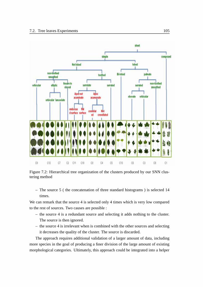
7.2. Tree leaves Experiments 105
Figure 7.2: Hierarchical tree organization of the clusters produced by our SNN clus-tering method
– The source 5 ( the concatenation of three standard histograms ) is selected 14
times.
We can remark that the source 4 is selected only 4 times which is very low compared
to the rest of sources. Two causes are possible :
– the source 4 is a redundant source and selecting it adds nothing to the cluster.
The source is then ignored.
– the source 4 is irrelevant when is combined with the other sources and selecting
it decreases the quality of the cluster. The source is discarded.
The approach requires additional validation of a larger amount of data, including
more species in the goal of producing a finer division of the large amount of existing
morphological categories. Ultimately, this approach could be integrated into a helper

106Chapter 7. Structuring visual contents with multi-source shared-neighbours
clustering
application to the analysis and into the establishment of morphological categories of
flora, including the flora being found in the tropics where a large number of species
remains to discover.
A second perspective would be to integrate this clustering method in an identification
system of species. The idea is to build as many binary classifiers as there are clusters
estimated by the clustering method. An image to be identified would be associated
with a set of outcomes. Afterwards each classifier measures the membership of the
image to the morphological categories. The following results could then be exploited
to develop a list of species most likely, those sharing the greatest number of similar
morphological categories.
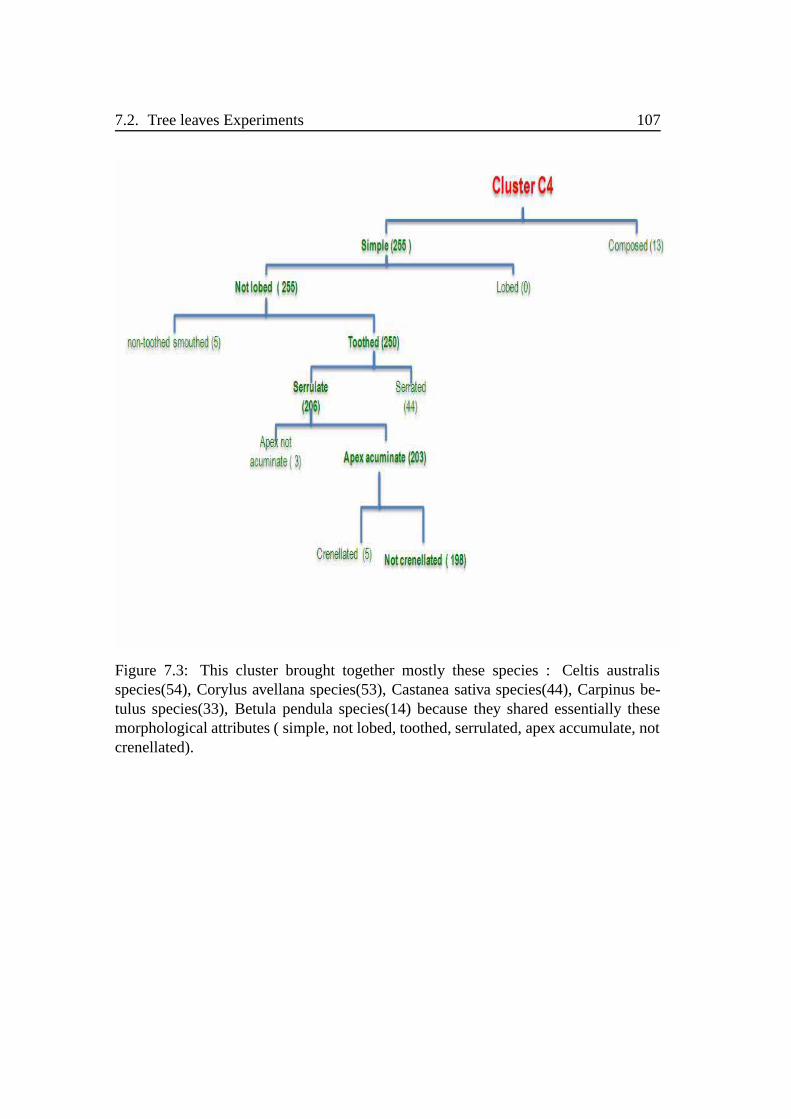
7.2. Tree leaves Experiments 107
Figure 7.3: This cluster brought together mostly these species : Celtis australisspecies(54), Corylus avellana species(53), Castanea sativa species(44), Carpinus be-tulus species(33), Betula pendula species(14) because they shared essentially thesemorphological attributes ( simple, not lobed, toothed, serrulated, apex accumulate, notcrenellated).
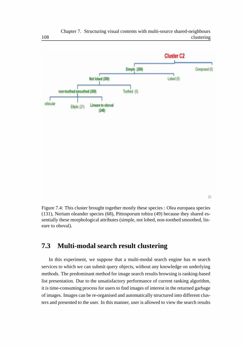
108Chapter 7. Structuring visual contents with multi-source shared-neighbours
clustering
Figure 7.4: This cluster brought together mostly these species : Olea europaea species(131), Nerium oleander species (68), Pittosporum tobira (49) because they shared es-sentially these morphological attributes (simple, not lobed, non-toothed smoothed, lin-eare to oboval).
7.3 Multi-modal search result clustering
In this experiment, we suppose that a multi-modal search engine has m search
services to which we can submit query objects, without any knowledge on underlying
methods. The predominant method for image search results browsing is ranking-based
list presentation. Due to the unsatisfactory performance of current ranking algorithm,
it is time-consuming process for users to find images of interest in the returned garbage
of images. Images can be re-organised and automatically structured into different clus-
ters and presented to the user. In this manner, user is allowed to view the search results

7.3. Multi-modal search result clustering 109
through a few clusters rather than mixed images. Such re-organisation is very effective
for browsing the search results. In the multi-modal case, images have a lot of proper-
ties which are quite different from a source of information to another. The goal is to
benefit from all available sources of information which helps to have more meaningful
information concerning the images. By considering all search services (information
sources) as simple oracles returning ranked lists of relevant objects, we can do a multi-
modal analysis and clustering especially towards exploiting the synergy between the
various media including text and visual information or between any other sources of
information.
Clustering approaches applied on different features have been studied severely before
but the originality of our work is the use of the shared neighbourhood clustering that
presents a lot of advantages (see Section 2.4.2) compared to the other clustering meth-
ods in a multi-source case where all the sources of information are tested with the
intention of selecting the optimal combination of sources for each cluster. All result-
ing clusters have not necessarily contrary to other previous work the same selected
sources. Figure 7.5 is an illustration of a multi-modal search clustering using only two
sources of information : visual and textual services.
Because it is difficult to have ground truth on real search engine, we simulate the
multi-modal clustering on the Wikipedia image dataset of ImageClef 2009 3. Initially,
this dataset is dedicated to multi-modal retrieval evaluations but we benefit here from
the provided annotations to build a text-image search results clustering task.
Among the full 150K images dataset, we keep only the images that have been effec-
tively annotated during the pooling procedure, i.e the images that have been manually
controlled as positive for at least one of the 44 query topics. The resulting dataset is
composed of 1582 images categorized in 44 clusters. Each image is associated with
textual information extracted from the initial Wikipedia web page (title, description,
etc).
We used two information sources, one textual information source based on the TF/IDF
similarity measure of PF/Tijah system [68]. One visual information source based on 5
global visual features (HSV Histogram [49], Hough histogram [49], Fourier histogram
[49], edge orientation histogram [49] and probability weighted RGB histogram) and
L1 metric as similarity measure.
We used the same F1 and AvgPurity metric as described before. Results are given
in Table 7.1. Using visual source, the clustering return more relevant categories than
3. http://www.imageclef.org/2009/wiki

110Chapter 7. Structuring visual contents with multi-source shared-neighbours
clustering
Figure 7.5: Illustration of a multi-modal search result clustering using visual and tex-tual sources of information.
using textual source but clusters are less coherent. However, by combining the two
modalities, the F1 measure and the average purity increase. The source selection step
during the clustering process makes the results better than each single source. Clus-
ters produced by selecting both of visual and textual sources are more semantically
and visually coherent. The remaining clusters that select the visual source are visually
coherent but not semantically while clusters using textual source are visually hetero-
geneous but semantically relevant.
Figure 7.6 is a part of the clustering result (the first four clusters) ranked in decreasing
order quality. The oracle selection step opt for the optimal sources for every cluster.
As it is shown, the first cluster (a) is semantically and visually coherent. For the second
cluster (b), the textual source is selected because it is considered better than the combi-
nation with the visual source. Images are visually different but refer all to the keyword
“Stamp”. However, the third cluster (c) is visually consistent by semantically have a
little sense. In the last cluster (d), images refer to the word “Dog” but are visually very

7.4. Visual object mining 111
heterogeneous.
Visual and Textual sources Textual source Visual source
F1 0.63 0.30 0.62AvgPurity 0.55 0.51 0.35
Table 7.1: F1 and AvgPurity measures for the Sub set of Wikipedia ImageClef 2009.
7.4 Visual object mining
Keyword queries are usually ambiguous especially when they are short. This am-
biguity often leads to unsatisfying search results. Many queries like “apple” covers
several different topics: fruit, computer, smart-phone,and so on. In some cases, users
prefers to have a list of the different categories returned in the search result than a
mixed images with divers categories. The goal in this application is not to provide all
clusters of the search results but a summarized list of the different topics of the query.
Users can after easily figure out what they are exactly searching by selecting the target
topic. Showing image from the target category in which the user is truly interested is
much more effective and efficient than returning all clusters or all mixed images.
We performed a visual object mining experiment based on Caltech256 dataset. Ini-
tially, this dataset was dedicated to supervised objects classification so that unsuper-
vised clustering over the 256 classes provides too weak results for consistent analysis.
We thus used this dataset in a different way to evaluate visual objects discovery in small
image sets. This experiment is a simulation of a visual object mining and the goal is to
evaluate the ability of our method to retrieve the categories. We collected 5 subsets of
the Caltech256 dataset. Each subset is constructed from 10 random categories and 20
random images selected from the whole database. Each subset is typically like images
that we could get from a previous textual search. The size of each subset is respectively
1792, 1581, 1221, 2098 and 1390 images. We used the same 5 global visual features as
described in the previous experiment. Table 7.2 shows the performance comparison of
our method and each visual feature. By combining the global visual features together,
the F1 measure is better than that of each source. The “Fourier Histogram” performs
better than the others mono-sources but remains lower than multi-source case.
The average selection of each visual global feature is reported in Table 7.3. As it is
shown, the “HSV Histogram feature” is the most selected feature on average in this
experiment. However, the “Prob-weighted Histogram RGB” feature is never selected

112Chapter 7. Structuring visual contents with multi-source shared-neighbours
clustering
(a) Cluster Number 1: Oracle selection = Textual and visual sources ,SSI(C1,F)= 328.936
(b) Cluster Number 2: Oracle selection = Textual source
(c) Cluster Number 3: Oracle selection = visual source
(d) Cluster Number 4: Oracle selection = Textual source
Figure 7.6: First four Clusters of the Wikipedia’s subset clustering using visual andtextual sources .

7.5. Image clustering based on multiple randomized visual subspaces 113
when it is combined with all the visual features because it provides no more relevance
to the clusters.
DB1 DB2 DB3 DB4 DB5 Avg
Multi-source 0.38 0.37 0.56 0.27 0.57 0.43HSV Histogram 0.36 0.21 0.42 0.13 0.53 0.33
Hough Histogram 0.36 0.24 0.31 0.22 0.47 0.32Fourier Histogram 0.35 0.34 0.54 0.24 0.50 0.39
Edge Orientation Histogram 0.35 0.24 0.35 0.15 0.54 0.32Prob-weighted Histogram RGB 0.36 0.21 0.42 0.13 0.46 0.31
Table 7.2: Clustering results on F1 measure for the Sub sets of Caltech256.
Visual global feature Average selection
HSV Histogram 0.56Hough Histogram 0.26Fourier Histogram 0.14
Edge Orientation Histogram 0.17Prob-weighted Histogram RGB 0
Table 7.3: Average selection of each global visual feature in the Caltech Experiment.
7.5 Image clustering based on multiple randomized vi-sual subspaces
7.5.1 Proposed method
Recently, researchers have begun paying attention to combine a set of individual
classifiers in order to improve the overall classification accuracy. An ensemble of clas-
sifiers must be both diverse and accurate in order to improve the accuracy of the whole.
Most of them use a simple vote from the output of each classifier to decide the final
result. However, in our case, we combine the lists of K-NN and apply our single clas-
sifier once.
The idea of our method is to determine multiple K-NN lists. Every K nearest neigh-
bours list is based on a random subset features selection. Then our oracle selection
step selects the best K nearest neighbours among the available list of K-NN and thanks
to the reshaping operation increases the accuracy of the class prediction.
We select the random subset of features by sampling from the original set of features.
Each of the nearest neighbours list is computed using the same number of features,
has access to all the patterns in the original training set but only to a random subset of
114Chapter 7. Structuring visual contents with multi-source shared-neighbours
clustering
features.
Selecting different feature subsets is an attempt to make different and hopefully un-
correlated errors. However, there is no guarantee that using different features sets will
decorrelate the error because in high dimensional data, many of the dimensions are of-
ten irrelevant. These irrelevant dimensions can confuse clustering algorithms by hiding
clusters in noisy data but we think that our oracle selection step will make irrelevant
sources less selected than relevant ones which increase cluster’s quality.
In contrast to other dimensionality reduction techniques, like those based on projection
(e.g. principal component analysis) or compression (e.g. using information theory),
feature selection techniques do not alter the original representation of the variables,
but merely select a subset of them. Thus, they preserve the original semantics of the
variables, hence, offering the advantage of interpretation by a domain expert.
By using multiple subsets of features, our clustering approach tries to find clusters that
exist in multiple possibly overlapping subspaces. The corresponding sources of clus-
ters would indicate the key concept of the domain (keywords that are relevant for each
cluster). This information can be very useful for the user and help him to have an idea
of the cluster’s category.
Generate K-NN on a high-dimensional feature tends to be computationally complex.
For this reason, we search for a multiple K-NN on a subset of features instead of
searching the K-NN on all the features. A high-dimensional feature like Bag-Of-
Features allows to represent every image as a set of visual words, hence making it
possible to describe them with a weighted vector. We choose this high-dimensional
feature to experiment our method. The oracle selection and reshaping steps combine
neighbours from multiple subset features to build the best K-NN in order to increase
the quality of the candidate cluster. The redundant clusters elimination is then applied
on the final K-NN lists to produce final clusters. Each cluster is constructed according
to its optimal subset of features.
7.5.2 Experiment
We tested our proposed multiple random subset features clustering on a small sub-
set of the large hand-labelled ImageNet dataset. ImageNet is an image dataset orga-
nized according to the WordNet hierarchy. Each meaningful concept in WordNet, is
described by multiple words or word phrases. It is used on “PASCAL Visual Object
Classes Challenge 2010” (VOC2010) 4.
4. http://www.image-net.org/challenges/LSVRC/2010/index

7.5. Image clustering based on multiple randomized visual subspaces 115
We use bag of visual words as features for our experiment. We extract 30 random
subset features of the bag-of-words. Each subspace represents 10% of the full space.
We use a sampling with replacement (a feature can be selected more than once). We
then compute the k-nearest neighbours of each image according to the corresponding
subset of features. Each K-NN according to a random subset feature is considered as
a source of information.
We extract from the validation database of ImageNet (that consists of 200,000 pho-
tographs, collected from flickr and other search engines, hand labelled with the pres-
ence or absence of 1000 object categories) 500 items clustered in 10 categories
Table 7.4 reports the clustering results using on the one hand the full space and on
the other hand a multiple random subset features varying from 2 to 30 sources. The
results demonstrate that using multiple subset features is better than using the whole
high dimensional feature. By using a number of sources at least equal to nearly 4
sources, the F1 measure, the average purity and the cosine measure exceed those of
full space. As expected the performance of our method greatly increase by combining
different source of information even if they are produced from the same feature. The
reshaping step improves the quality of clusters by adding other elements from other
sources. With 30 subspaces, The F1 measure, the average purity measure and the Av-
erage Cosine (F1=0.66, AvgPurity=0.26, AvgCosine = 0.33) increase and particularly
the F1 measure was approximately doubled compared respectively to F1 measure of
the full space (F1=0.30).
F1 AvgPurity AvgCosine Measure
Full Space 0.30 0.23 0.202 sources 0.17 0.17 0.164 sources 0.32 0.19 0.216 sources 0.54 0.21 0.238 sources 0.53 0.20 0.25
10 sources 0.66 0.21 0.2820 sources 0.66 0.23 0.2930 sources 0.66 0.26 0.33
Table 7.4: Multiple Random Subset features clustering result on ImageNet subset

116Chapter 7. Structuring visual contents with multi-source shared-neighbours
clustering

Chapter 8
Structuring visual content withbipartite shared-neighbours clustering
8.1 Visual objects Discovery and Object-based VisualQuery Suggestion
8.1.1 Introduction
State-of-the-art visual search systems allow to retrieve efficiently small rigid ob-
jects in very large datasets. They are usually based on the query-by-window paradigm:
a user selects any image region containing an object of interest and the system returns
a ranked list of images that are likely to contain other instances of the query object.
User’s perception of these tools is however affected by the fact that many submitted
queries actually return nothing or only junk results (complex non-rigid objects, higher-
level visual concepts, etc).
In this chapter, we address the problem of suggesting only the object’s queries that
actually contain relevant matches in the dataset. This requires to first discover accu-
rate object’s clusters in the dataset (as an off-line process); and then to select the most
relevant objects according to user’s intent (as an on-line process). We therefore intro-
duce a new object’s instances clustering framework based on a major contribution: a
bipartite shared-neighbours clustering algorithm that is used to gather object’s seeds
discovered by matching adaptive and weighted sampling. We study a bipartite graph in
the context of object’s discovery. Experiments show that this new method outperforms
state-of-the-art object mining and retrieval results on the Oxford Building dataset. We
finally describe two object-based visual query suggestion scenarios using the proposed
framework and show examples of suggested object queries.
118 Chapter 8. Structuring visual content with bipartite shared-neighbours clustering
8.1.2 New visual query suggestion paradigm
Large-scale object retrieval systems have demonstrated impressive performance in
the last few years. The underlying methods, based on local visual features and effi-
cient indexing models, can retrieve accurately small rigid objects such as logos, build-
ings or manufactured objects, under varying view pose and illumination conditions
[131, 130, 80, 99, 132, 25, 84]. Therefore online object retrieval is now achievable up
to 1 M images with a state-of-the-art computer [80].
From the usage point of view, these methods are usually combined with a query-by-
window search paradigm. The user can freely select a region of interest in any image,
and the system returns a ranked list of images that are the most likely to contain an
instance of the targeted object of interest [132]. This paradigm has however several
limitations related to user’s perception: (i) When no (or very few) other instances of
the query object exist in the dataset, the system mostly returns false positives making
the user uncomfortable with the results. Indeed, he does not know if there are actually
no other instances of the query object or if the system did not work correctly. (ii) When
the user selects a deformable or complex object that the system is actually not able to
retrieve, the system mostly returns false positives as well. As the user can freely select
any object, this appears very frequently leaving the user with a bad impression of the
effectiveness of the tool.
The second remark is even more critical if the user believes that the system can re-
trieve any semantically similar objects (e.g. object categories or visual concepts such
as cats or cars). We do not argue here that such queries will never be solved effectively
in the future. We just emphasize that bridging the gap between user’s understanding
of the system and the actual capabilities of the underlying tools is essential to make
it successful in a real world search engine. A first possible solution to address these
limitations would be to use some adaptive thresholding method, allowing only rele-
vant results to be filtered, and possibly returning no results if none are found. The a
contrario method of [84], for instance, allows the actual false alarm rate of rigid object
instances retrieval to be controlled very accurately. But still, as the user can select any
region of interest, the system might return no results in many cases and leave the user
disappointed.
We propose to solve these user perception issues by a new visual query suggestion
paradigm. Rather than letting the user select any region of interest, the system will
suggest only visual query regions that actually contain relevant matches in the dataset.
By mining offline object instances in the dataset, it is indeed possible to suggest to

8.1. Visual objects Discovery and Object-based Visual Query Suggestion 119
the user only query objects having at least a prefixed number of instances in the col-
lection. Figure 8.1 illustrates such suggested objects in several images. When a user
clicks on a highlighted region, the system returns only the images containing other
object instances of the same discovered cluster. From a user perception point of view,
the proposed paradigm is very different to the window query paradigm. Indeed, since
all suggested objects mostly return correct results, the user might rather perceive them
as visual links (or hyper-visual links by analogy to hypertext links). To the best of
our knowledge, this is the first work to detail a method for object-based visual query
suggestion. Unlike existing approaches, the links produced by our method are not sim-
ilarity links between images, but rather links between automatically localized images
containing instances of the same rigid object. These object-based visual links can be
used in many different retrieval paradigms. In this paper, we focus on two visual query
suggestion scenarios showing the potential of the proposed method :
Mouse-over visual objects suggestion: when the user moves or hovers the mouse
cursor over a particular image, the system suggests object queries by highlighting the
object instances present in the image. The suggested objects do not depend on the
preliminary textual query but are guaranteed to match some other instances in the col-
lection (when the user clicks on one of them).
Text-aware visual objects suggestion: After a user submits a text query, the most
frequent visual items discovered in the result list are suggested as new object-based
visual queries (typically displayed as some clickable thumbnails on top of the result
GUI). Images containing other instances of the suggested object are returned if the
user clicks one.
Simple as it seems to be, moving from the free window-query paradigm to the object’s
suggestion paradigm is not trivial. Indeed, it first requires to discover accurate object’s
clusters in the dataset (typically as an off-line process), without any supervision and
without knowledge on the location and the extent of the objects.
Therefore, this chapter introduces a new object’s instances clustering framework based
on two main steps:
Object’s seeds discovery with adaptive weighted sampling: this step, proposed in
[102], allows to discover small and rigid repeated patterns in the collection by ran-
domly querying small image patches with an efficient geometric matching. In the next
section 8.1.4, we summarize the work done by [102] and we use their result as input
for our experimentations.
Bipartite shared-neighbours clustering: This proposed algorithm allows building
full object’s models by clustering the previously discovered object’s seeds (Section

120 Chapter 8. Structuring visual content with bipartite shared-neighbours clustering
8.1.4).
Object’s clusters will be used for the object-based visual query suggestion and for the
object retrieval. Note that shared neighbours clustering methods were never been stud-
ied before in the case of bipartite graph and never been applied to object’s discovery
either.
Figure 8.1: Discovered visual objects are displayed as links on which the user clicksto focus the retrieval on this specific object represented by a link-object.
8.1.3 Proposed visual query suggestion
Visual Query Suggestion was originally suggested in [184] by extension to Textual
Query Suggestion methods that are now used in most existing search engines. The
claim of the authors was that text-based predictive suggestion methods might some-
times not accurately express the intent of the users. By adding to the textual sug-
gestion a set of representative pictures, the user can express his specific search intent
more clearly. Their method was mainly based on global visual similarities using a
joint text-image re-ranking for the retrieval. Our method differs in two main points:
(i) we suggest purely visual queries (although the suggested queries can be computed
according to the results of a textual query) (ii) the suggested visual queries represent
object(s) in images and not global visual concepts associated to each image.
Beyond large-scale object retrieval methods discussed in the introduction [131, 130,
80, 99, 132, 25, 84], our work is more related to object-based image clustering and
unsupervised object mining techniques [24, 133, 134, 163]. Object-based image clus-
8.1. Visual objects Discovery and Object-based Visual Query Suggestion 121
tering attempts to cluster images that contain instances of the same object. Our ob-
jective differs in that we do not attempt to build image clusters but rather clusters of
image regions containing instances of the same object. The problem to be solved is
more challenging since the image regions to be clustered are not predefined entities (as
images are). Therefore, image regions need to be segmented and clustered at the same
time. This is basically what object mining methods are aimed at.
Many objects discovery method rely on graph-based clustering methods. They usually
include a preliminary step allowing to discover object’s seeds, i.e. spatially stable im-
age regions in the collection. The main objective of this step is to build a matching
graph that will be processed afterwards to cluster images or discover object instances.
Similarly to some works using graph-based object mining mentioned in Section 3.3,
our framework rely on two main steps: (i) building a matching graph by mining spa-
tially consistent object seeds by using the method of [102] and (ii) post-processing the
graph to build clusters of object’s instances. But contrary to these methods, we for-
mulate the problem as a bipartite graph clustering issue. Images are indeed considered
as a first set of nodes, while object’s seeds form a second disjoint one. Next section
details the method used to discover object seeds and build the matching graph.
8.1.4 Building a matching graph and mining visual object seeds
As stated before, state-of-the-art large-scale object retrieval systems usually com-
bine efficient indexing models with a spatial verification re-ranking stage to improve
query performance [84, 130]. In the method that we used [102], authors suggested to
use a such accurate two-stage matching strategy for building the input matching graph.
The problem then rather becomes a sampling issue: how to effectively and efficiently
select relevant query regions while minimizing the number of tentative probes. For
this, they introduced an adaptive weighted sampling strategy.
Sampling is a statistical paradigm concerned with the selection of a subset of indi-
vidual observations within a population of objects intended to yield some knowledge
about the population without surveying it entirely. If all items have the same proba-
bility to be selected, the problem is known as uniform random sampling. In weighted
sampling methods [123], the items might be weighted individually and the probabil-
ity of each item to be selected is determined by its relative weight. In conventional
sampling designs, either uniform or weighted, the selection for a sampling unit does
not depend on the observations made during previous surveys. On the other hand,
Adaptive sampling [152] is an alternative strategy aiming at selecting more relevant

122 Chapter 8. Structuring visual content with bipartite shared-neighbours clustering
sampling regions based on the results observed during the previous surveys.
The object seeds discovery method that we used is composed of three main stages
processed at each iteration: Adaptive Sampling of a query image region, Search of the
selected local query region and Decision of whether this query region might be con-
sidered as an object seed in the final output matching graph. The full algorithm repeats
these 3 steps T times until a fixed number of seeds has been found.
More formally, let Ω be an input dataset of N images Ii, i ∈ 1, ...,N.
Each image Ii is represented by a set of Ni local visual features fi, j (typically SIFT
[108]) localized by their position Pi, j. N f = ∑Ni=1 Ni is the total number of features fi, j.
Each local feature fi, j is associated with a fixed candidate query region Ri, j defined as
the bounding box centred around Pi, j, with height Hi, j and width Wi, j.
Finally, after T tentative probes, the algorithm outputs a set S of |S| ≤ T seeds S j. Each
seed corresponds to a spatially verified frequent visual pattern. A seed is associated
with a query image region R jq and a set of Mj matching regions R j
m, m ∈ 1, ...,Mj.
The more the number of tentative probes is, the more a frequent object is likely to be
considered as a seed. As this step of building matching graph is not our contribution,
we will not detail more. See [102] for further explanation.
Although the discovered seeds correspond to consistent repeated patterns in the
collection, they can still not be considered as full objects: (i) by construction, a seed
usually covers only a subpart of an object instance with a loose localization, (ii) fur-
thermore, due to the imperfect recall of the retrieval, a discovered seed matches only a
subset of all instances in the dataset, (iii) finally, the more frequent an object is in the
collection, the more redundant the discovered seeds are. Building accurate and com-
plete object’s model therefore requires to group all seeds belonging to the same object.
This cannot be done according to the visual content of the seeds, since two seeds with
distinct visual contents might still be two subparts of the same object. A more intuitive
alternative is to group seeds that are matching correlated contents in the dataset, which
can be formulated as a bipartite clustering problem. Figure 8.2 illustrates our proposed
method to group seeds representing the same object.
Let us denote as G = (X ;E) = (I,S;E) the bipartite matching graph resulting from the
object’s seeds discovery, with
I = {Ii}i∈[1,N]
the vertex set representing the images of the collection,
S ={
S j}
j∈[1,|S|]the vertex set of the discovered seeds, X = I ∪ S and I ∩ S = /0. Each directed edge

8.1. Visual objects Discovery and Object-based Visual Query Suggestion 123
S1 S2 S3 S4 S5 S6 S7 S8 S9 …
I1 0.96 0 0.14 0.67 0.45 0 0.78 0 0.58 ...
I2 0 0.5 0.34 0 0.26 0.79 0.63 0.24 0 …
I3 0.19 0.24 0 0.56 0 0 0 0.82 0.74 ...
I4 0.41 0 0.52 0.53 0 0.75 0.69 0 0.21 ...
I5 0.33 0.09 0 0.39 0 0.44 0 0.22 0 ...
I6 0 0.66 0 0 0.75 0 0.67 0 0.9 ...
… … … … … … … … … ... ...
… … … … … … … … … … ...
Object seeds
Imag
es
Bipartiteclustering
Cluster 1 Cluster 2
S1 S2 S3 S4 S5 S6 S7 S8 S9 …
I1 0.96 0 0.14 0.67 0.45 0 0.78 0 0.58 ...
I2 0 0.5 0.34 0 0.26 0.79 0.63 0.24 0 …
I3 0.19 0.24 0 0.56 0 0 0 0.82 0.74 ...
I4 0.41 0 0.52 0.53 0 0.75 0.69 0 0.21 ...
I5 0.33 0.09 0 0.39 0 0.44 0 0.22 0 ...
I6 0 0.66 0 0 0.75 0 0.67 0 0.9 ...
… … … … … … … … … ... ...
… … … … … … … … … … ...
Object seeds
Imag
es
Figure 8.2: Illustration of the proposed method to suggest object-based visual queriesin the image I4. S2,S5 and S9 belong to the cluster representig the same object by usingthe bipartite clustering. S3,S6 and S8 represent seeds belonging to the second object inthe image I4.
ei, j ∈ E has a starting point in S, an endpoint in I and a weight wi, j corresponding to
the matching score returned by the a contrario normalization method (wi, j = 0 means
that no edge connects seeds S j to image Ii). The advantage of this bipartite represen-
tation it to allow formulating our seeds clustering objective as a co-clustering problem
(or dual subset clustering [178]).
We indeed aim to find object clusters On = (Sn, In) with Sn ⊂ S being the subset of
seeds modelling a given object and In ⊂ I being the subset of images containing in-

124 Chapter 8. Structuring visual content with bipartite shared-neighbours clustering
stances of the object. An ideal object cluster is the one whose seeds are matching on
the same images. It is important to notice the advantage over previous object mining
methods using a single image-oriented matching graph [134, 24, 4, 63]: a given image
can be accurately affected to several object clusters (when it contains instances of dis-
tinct objects). Furthermore, each object cluster is composed of a unique set of seeds
associated with localized matching regions. As discussed in the next subsection, this
will be useful for display purposes within our visual query suggestion scenarios.
Solving the bipartite clustering problem is not a trivial task. Some previous works
proposed using spectral based techniques in the context of text documents clustering
[177, 178]. These methods are useful to partition bipartite graphs in a prefixed number
of balanced clusters but are not appropriated to our problem. The number of objects
to be discovered as well as the number of seeds to be grouped within each object can
indeed be highly variable. In addition, the results are very sensitive to the parameters
used by these methods. This is why we proposed to use our new bipartite clustering
algorithm described in Chapter 6 and inspired by Shared Nearest Neighbors (SNN)
clustering methods [73, 65, 139].
The principle of our method as well as SNN algorithms in general is to group items not
by virtue of their pairwise similarity but by the degree to which their neighbourhoods
resemble one another. They are well known to overcome several shortcomings of
classical clustering methods, notably high-dimensionality and similarity metrics limi-
tation.
8.1.5 Object-based visual query suggestion
For each of the two visual query suggestion paradigms described in the introduc-
tion, we answer the following questions: What do we suggest? How do we display the
suggestions? What do we return when the user clicks on a suggested object?
– Mouseover visual objects suggestion : For any image I j ∈ I, we suggest
queries. The number of these queries is equal to the number of clusters having
I j in their dual image set. Each cluster is represented by a rectangular window
computed from the set of all regions that have been matched by the seeds of
the cluster. Taking the bounding box of all matching regions would however be
affected by outlier matches. We rather keep the bounding box of all pixels that
are covered by at least 2 matching regions, as illustrated in Figure 8.3. When
the user clicks on one of the suggested objects, we return a ranked list of images
according to their intersection to the selected object (i.e. the number of seeds

8.2. Experiments 125
matching with it or the sum of the corresponding matching weights).
Figure 8.3: Steps to obtain the suggested visual object on an image from BelgaLogos:i) selecting the bounding box, ii) intersection of bounding box , iii) keeping only theregion that have been covered by at least two bounding box. The final result is thesuggested object.
– Text-aware visual objects suggestion: We suppose that an external text-based
search did already return a subset Ix ⊂ I of images. We then select as suggested
query objects the top M clusters of the dataset having the greatest intersection
between the images in their dual representation and the text-based result list (i.e.
the clusters representing the most frequent objects in the result list). Each sug-
gested query object is displayed at the top of the search interface by a single
representative thumbnail. This is done by first seeking the image that has the
most intersection with the cluster (by mean of the number of seeds matching it)
and then by cropping the object of interest in this image with the same procedure
as the one described in the previous mouseover scenario. An illustration of re-
sulting visual queries is given in Figure 8.4 for Oxford Buildings dataset. When
the user clicks on one of the suggested object, we return as before a ranked list
of images according to their intersection to the object.
8.2 Experiments
8.2.1 Experimental setup
Our method is demonstrated on three databases:
– Oxford Buildings: This dataset is described in 1 and consists of 5062 images of
buildings from Oxford and miscellaneous images all retrieved from Flicker. A
ground-truth is provided for 55 queries (11 different landmarks in Oxford). We
describe the corpus with 30 million SIFT [108] features.
1. http://www.robots.ox.ac.uk/ vgg/data/oxbuildings/

126 Chapter 8. Structuring visual content with bipartite shared-neighbours clustering
Figure 8.4: Some object clusters discovered in the Oxford Buildings Dataset. The top4 rows clusters are in the ground truth. The fifth first columns are seeds examples ofthe cluster and the last column represents the suggested query object of each cluster.
– BelgaLogos: This dataset 2 is composed of 10,000 images. The images have
been manually annotated for 26 logos. A given image can contain one or several
2. http://www-rocq.inria.fr/imedia/belga-logo.html

8.2. Experiments 127
logos or no logo at all. We described this corpus with 38 millions of SIFT.
– GoogleCrawl: To illustrate the text-aware visual objects suggestion paradigm,
we created a small dataset crawled from Google Image search engine using the
five following queries: Metallica Concert, Green Peace, Disney, Khadafi, and
World Cup. We described this dataset with 12 millions of SIFT.
For all experiments, the number of | S | of seeds was set to 5K. Note that this vocabulary
size is strongly lower than the sizes used by common bag-of-visual-word methods
applied on Oxford Buildings dataset.
8.2.2 Clustering Performance evaluation
We first compared our clustering method to state-of-the-art objects mining methods
[134, 24] on Oxford Buildings dataset. We used the same evaluation protocol as [134]
and [24]: for each landmark, we found the cluster containing the most positive (Good
and OK) images of that landmark and computed the fraction of positive ground truth
images in this cluster.
Table 8.1 summarizes the results of our method and reproduces the results reported by
Philbin et al. [134] and Chum et al. [24]. It shows that our method gives on average
better performances than these two methods. It is clear that the overall gain of our
method relies mainly on the two categories “Ashmolean” and “Magdalen” where other
methods do not achieve good results. For “Ashmolean”, we scored a MAP of 0.9095
which is high compared to the best score (MAP= 0.68) of both Philbin et al. [134] and
Chum et al. [24]. For “Magdalen” category, we scored a MAP of 0.7634 which is 3
times the score found by the best result (MAP =0.204 ) of both compared methods.
The worst result we found is equal to 0.5847 for the “Balliol” category while the worst
one for Philbin et al. [134] is equal to 0.204 and for Chum et al. [24] is equal to 0.0556
for the same category “Magdalen”.
This can be explained by the fact that these two methods combine bag-of-words in-
dexing models with spatial verification re-ranking stage to improve query performance
which gives a bad result if the initial results returned by the bag-of-words method are
very bad while in our case we discover spatially verified visual words. The geometric
consistency of the features points between patches make them consistent. So even if
the building takes a small part in the image, by using small consistent objects, we can
have cluster images that can be globally different but all containing the same object.

128 Chapter 8. Structuring visual content with bipartite shared-neighbours clustering
GroundTruth Object Philbin et al. [134] Chum et al. [24] Our Proposed Method
All Souls 0.937 0.9744 0.9187Ashmolean 0.627 0.68 0.9095Balliol 0.333 0.3333 0.5847Bodleian 0.612 0.9583 0.663Christ Church 0.676 0.8974 0.599Cornmarket 0.651 0.6667 0.7449Heterford 0.705 0.9630 0.957Keble 0.937 0.8571 1Magdalen 0.204 0.0556 0.7634Pitt Rivers 1 1 1RadCliffe Camera 0.973 0.9864 0.9087
Average 0.696 0.7611 0.8226
Table 8.1: A comparison of the MAP clustering’s results for the 5K Oxford Buildingsdataset.
8.2.3 Retrieval performance evaluation
To evaluate the accuracy of our visual query suggestion method in terms of retrieval
performances, we computed different MAP on Oxford Buildings dataset. We first
evaluated the retrieval only for the common 55 queries, provided with their bounding
boxes. We therefore select only the object’s clusters discovered by our method that
have one of the 55 image queries in their dual image set (as if the mouseover query
suggestion scenario was applied to these images). In the first case, we considered as
clicked queries only the object’s clusters having a match within the bounding box. We
then returned the list of matching images sorted by decreasing order of the matching
score (i.e. the sum of weights wi, j over all seeds belonging to the selected clusters).
Detailed results for each landmark are presented in Table 8.2. We also give in Table
8.3 the MAP over all queries compared to the retrieval results reported in Jegou et al.
[80] and Philbin [130]. The results show that our method outperforms both methods.
To demonstrate that our proposed method is not only good for the common 55
queries but for any image, we then evaluated the retrieval in all images annotated to 1 in
the groundtruth. Since we do not have bounding box with these images, we considered
as clicked queries all objects suggested in these images. We also did the same for the
55 common queries for fair comparison. Results are reported in Table 8.4. They show
that the MAP remains very good whereas some of the images belonging to the full
groundtruth contain very small instances of the building, more partial views and more

8.2. Experiments 129
GroundTruth Object MAP
All Souls 0.967Ashmolean 0.9045
Balliol 0.5594Bodleian 0.922
Christ Church 0.8821Cornmarket 0.7449Heterford 0.9631
Keble 0.8736Magdalen 0.7603Pitt Rivers 1
RadCliffe Camera 0.9172
Average 0.8631
Table 8.2: Detailed MAP for the 12 landmarks of Oxford Buildings
Jegou [80] Philbin [134] Our method
MAP 0.74 0.82 0.86
Table 8.3: A comparison of the MAP retrieval’s results for the 5K Oxford.
complex view points. That is important in the sense that it proves the feasibility of our
new object’s suggestion paradigm. Whatever the object and the image in which we
suggest a query, the returned results will be as good as if the user had selected himself
one of the 55 windows queries.
55 queries (withbounding box)
55 queries(without
bounding box)
All images inground truth
MAP 0.86 0.84 0.836
Table 8.4: MAP retrieval’s results of the 55 queries compared to all images annotatedto 1 of the ground truth. This means that whatever the object and the image in whichwe suggest a query, the returned results will be as good as if the user had selectedhimself one of the 55 windows queries
We finally computed some statistics on the produced clusters to evaluate the com-
pleteness of the suggested visual queries. Figure 8.5 gives the percentage of images

130 Chapter 8. Structuring visual content with bipartite shared-neighbours clustering
having equal or more than a number of suggested query objects denoted as m, for in-
creasing values of m. It shows that when using only 5K seeds, 42 percent of the images
have at least one suggested visual query. Remember that the number of seeds being a
parameter of the method a more complete coverage can be simply obtained by running
the seed’s discovery algorithm longer. But, more we iterate, more we discover smaller
and no frequent objects.
10
20
30
40
50
60
70
80
90
100
0 2 4 6 8 10 12 14
Per
cent
age
of im
ages
Number of suggested query objects (m)
Figure 8.5: Histogram of the percentage of images that have more than m suggestedquery objects.

8.2. Experiments 131
8.2.4 Visual query suggestion illustration
To illustrate qualitatively our suggested visual queries on other dataset, we used
the BelgaLogos and GoogleCrawl datasets. The text-aware visual objects suggestion
scenario is illustrated using the GoogleCrawl dataset. Figure 8.6 shows the top 3 sug-
gested objects for each of the 5 text queries. To better understand what is behind such
suggested objects we also provide in Figure 8.7, for 4 suggested queries, the top 3
images returned when the user clicks on them.
Figure 8.8 illustrates the Mouseover visual objects suggestion scenario on BelgaL-
ogos dataset. The two first images are illustrations of images having two visual queries.
The three last ones illustrate 3 other images with only one suggested visual query. The
right column gives the top 3 returned images for each suggested query.
Metallicaconcert
Greenpeace
Disney
Khadafi
World Cup
Figure 8.6: Some Suggested visual queries for each of the text-queries in the set ofimages crawled from Google Images.

132 Chapter 8. Structuring visual content with bipartite shared-neighbours clustering
Figure 8.7: Some suggested queries and the top three images returned for each one.
8.3 Conclusion
As future work, we plan to study the influence of the size and shape of the query
region in the object seeds generation. Moreover, we plan to study the impact of the
size of discovered seeds on the performance and accuracy of our approach.

8.3. Conclusion 133
Figure 8.8: Some discovered object clusters in BelgaLogos.

134 Chapter 8. Structuring visual content with bipartite shared-neighbours clustering

Part IV
Conclusion and perspectives


Chapter 9
Conclusion
9.1 Synthesis and conclusion
This thesis address the problem of content structuring and mining by using shared
nearest neighbours clustering. Our motivation was that most classical data cluster-
ing often force particular choice of data representation and similarity measures. Such
assumptions are particularly problematic in multimedia context that usually involves
heterogeneous data and similarity measures. For this reason, we investigate new
clustering paradigms and algorithms based on the principle of shared nearest neigh-
bours (SNN) that are suitable to overcome data complexity, heterogeneity and high-
dimensionality.
First, we proposed to revisit existing state-of-the-art shared neighbours methods in two
points. We first introduce a new SNN formalism based on the theory of a contrario de-
cision. This allows us to derive more reliable connectivity score that is used to select
the optimum neighbourhoods. The advantage of using this a contrario significance
score is that it not biased to the size of the clusters and it is interpretable. The idea is
to select the best neighbourhood for each item and then to eliminate redundant candi-
date clusters by using a greedy strategy (beginning by the best ones) and a reshaping
step that allows to add relevant items to final clusters from the deleted ones. We also
proposed a new factorization algorithm for speeding-up the intensive computation of
the required shared neighbours matrices. By using synthetic data, we demonstrated
that our proposed method is able to select the best neighbourhood in presence of noisy
source of K-nearest neighbours. Compared to the popular spectral clustering of Ng,
Jordan and Weiss [121], we showed that our method is more robust and less sensitive
to the size of the input graph.
The second contribution of this thesis is a generalisation of the proposed SNN cluster-

138 Chapter 9. Conclusion
ing approach to the multi-source case. The main originality of our approach is that we
introduced an information source selection step in the computation of the candidate
cluster scores. Any arbitrary item set is thus associated with its own optimal subset of
modalities maximizing a normalized multi-source significance measure. As shown in
the synthetic data experiments, this source selection step makes our approach not only
widely robust to the presence of locally outlier sources but also improves the quality
of the clusters. We concluded that efficiently combining sources can compensate the
weak quality of very noisy independent sources.
We applied our proposed multi-source shared nearest neighbours clustering to visual
content structuring in different applications. In the tree leaves experiment, we aimed
to help botanists to identify and formalize the useful morphological categories to dis-
tinguish species. The goal of our second multi-source application was to structure a
content search results. By considering the visual and the textual informations of im-
ages, we obtained clusters that selected both of visual and textual sources and they
were semantically and visually coherent. The remaining clusters that selected the vi-
sual source were visually coherent but not semantically while clusters using textual
source were visually heterogeneous but semantically relevant. Such re-organisation is
very effective for browsing the search results and very meaningful for users that has
the information why images are grouped together. In the third experiment “visual ob-
ject mining”, we demonstrated that thanks to our source selection step, we can have
some statistics about the used sources which can help users to select the best ones.
Finally, we focused our work to how extend SNN clustering to the context of bipartite
k-NN graphs i.e. when the neighbours of each item to be clustered lie in a disjoint
set. We introduced new SNN relevance measures revisited for this asymmetric context
and showed that they can be used to select locally optimal bipartite clusters. By using
synthetic data, we demonstrated that our bipartite SNN clustering performs the bipar-
tite spectral clustering by selecting relevant items during the candidate object cluster
creation. We applied our bipartite SNN clustering to visual object’s discovery based
on a randomly precomputed matching graph.
In comparison to recent work, experiments show that our method succeeds in increas-
ing the clustering and the retrieval effectiveness by discovering frequent consistent vi-
sual objects seeds and grouping those that matched on the same images in the dataset.
Based on the discovered objects, we also introduced a new visual search paradigm, i.e.
object-based visual query suggestion. The idea is to suggest to the user some relevant
objects to be queried as being the most frequent appearing in the full dataset or in a
subset filtered by previous queries. Rather than letting the user select any region of in-

9.2. Perspectives 139
terest, the system will suggest only visual query regions that actually contain relevant
matches in the dataset.
Along all these different applications in this PhD, we showed how the shared neigh-
bours information has the potential to be used on different data representation and
modalities and how our proposed methods whatever the context can deal with noisy
data and produces relevant clusters.
9.2 Perspectives
As our shared nearest methods proposed in this PhD demonstrated their potential
to select the optimal neighbourhood for each item, we plan to use these neighbourhood
to construct the input graph for spectral clustering. By these way, we produce a graph
easy to cluster and we improve the robustness of spectral method against noisy K-NN.
Such optimal neighbourhood could be used in many application such as recommen-
dation systems involving collaborative filtering or content-based filtering. P2P (peer
to peer) recommendation systems could, for instance, allow to maintain efficiently the
SNN graph through gossip-based operations.
In our next work, we will carry out more in-depth contribution on scalability which is
the main limit of our proposed SNN method. We plan to test two idea : the first is to
use hierarchical approach which deal with this problem and the second is to propose
a shared neighbour sensitive hashing. The main idea is to use a hash function chosen
such that points that share neighbours in the original space have a high probability of
having the same hash value.
Finally, we want to extend our SNN method to supervised classification. Using SNN
similarities might provide better performance than classical K-NN classifier, especially
in multi-source context.

140 Chapter 9. Conclusion

Chapter 10
Annexes
10.1 Hierarchical organisation of morphological prop-erties of leaves
– margin
– non-toothed and smooth
– toothed
– serrated
– serrulated
– crenellated
– Form sheet or leaflet
– Elliptical
– Orbicular
– obovate
– Linear
– Lanceolate
– Asymmetric
– Lobed
– lobed form
– not lobed
– palmate
– pinnate
– lobed
– Color dark/clear
– Matt/gloss surface

142 Chapter 10. Annexes
– Presence of thorns
– Ribs
– primary
– secondary
– Apex
– right
– convex
– acuminated
– emarginated
– lobed
– Base
– right or Cune
– concave
– convex
– concavo-convex
– complex
– decurrent
– roped
– lobed
– runcinated
– auriculated
Bibliography
[1] Charu C. Aggarwal, Alexander Hinneburg, and Daniel A. Keim. On the surpris-
ing behavior of distance metrics in high dimensional space. In Lecture Notes in
Computer Science, pages 420–434. Springer, 2001.
[2] Vasilis Aggelis and Vasilis Christodoulakis. Customer clustering using rfm anal-
ysis. In Proceedings of the 9th WSEAS International Conference on Computers,
ICCOMP’05, pages 2:1–2:5, Stevens Point, Wisconsin, USA, 2005. World Sci-
entific and Engineering Academy and Society (WSEAS).
[3] Rakesh Agrawal, Johannes Gehrke, Dimitrios Gunopulos, and Prabhakar
Raghavan. Automatic subspace clustering of high dimensional data for data
mining applications. pages 94–105, 1998.
[4] A. Anjulan and N. Canagarajah. A unified framework for object retrieval and
mining. Circuits and Systems for Video Technology, IEEE Transactions on,
19(1):63 –76, 2009.
[5] D. Barthelemy, N. Boujemaa, D. Mathieu, J.-F. Molino, A. Joly, Ph. Birnbaum,
P. Bonnet, E. Mouysset, H. Goeau, and V. Roche. The pl@ntnet project: plant
computational identification and collaborative information system. In XVIII
18th International Botanical Congress, Melbourne, Australia, Juillet 2011.
[6] Herbert Bay, Tinne Tuytelaars, and Luc Van Gool. Surf: Speeded up robust
features. In In ECCV, pages 404–417, 2006.
[7] Ron Bekkerman and Jiwoon Jeon. Multi-modal clustering for multimedia col-
lections. In CVPR. IEEE Computer Society, 2007.
[8] Mikhail Belkin and Partha Niyogi. Laplacian eigenmaps for dimensionality
reduction and data representation. Neural Computation, 15:1373–1396, 2003.
[9] Pavel Berkhin. A survey of clustering data mining techniques. Grouping Mul-
tidimensional Data, pages 25–71, 2002.
144 Bibliography
[10] Kevin Beyer, Jonathan Goldstein, Raghu Ramakrishnan, and Uri Shaft. When
is ”nearest neighbor” meaningful? In In Int. Conf. on Database Theory, pages
217–235, 1999.
[11] Chidansh Amitkumar Bhatt and Mohan S Kankanhalli. Multimedia data min-
ing: state of the art and challenges. Multimedia Tools and Applications,
51(1):35–76, 2010.
[12] David M. Blei, Andrew Y. Ng, and Michael I Jordan. Latent dirichlet allocation.
J. Mach. Learn. Res., 3:993–1022, March 2003.
[13] Matthew Brand and Kun Huang. A unifying theorem for spectral embedding
and clustering. 2003.
[14] M. R. Brito, E. L. Chavez, A. J. Quiroz, and J. E. Yukich. Connectivity of the
mutual k-nearest-neighbor graph in clustering and outlier detection. Statistics
& Probability Letters, 35(1):33–42, Aug 1997.
[15] Andrei Z. Broder. On the resemblance and containment of documents. In In
Compression and Complexity of Sequences (SEQUENCES97), pages 21–29.
IEEE Computer Society, 1997.
[16] Jeremy Buhler. Efficient large-scale sequence comparison by locality-sensitive
hashing. Bioinformatics, 17:419–428, 2001.
[17] Deng Cai, Xiaofei He, Zhiwei Li, Wei-Ying Ma, and Ji-Rong Wen. Hierarchi-
cal clustering of www image search results using visual, textual and link infor-
mation. In Proceedings of the 12th annual ACM international conference on
Multimedia, MULTIMEDIA ’04, pages 952–959, New York, NY, USA, 2004.
ACM.
[18] A. Colin Cameron, Jonah B. Gelbach, and Douglas L. Miller. Robust Inference
with Multi-Way Clustering. Technical Working Paper 327, National Bureau of
Economic Research, September 2006.
[19] Laurent Candillier, Isabelle Tellier, Fabien Torre, and Olivier Bousquet. Cas-
cade evaluation of clustering algorithms. In Johannes Frnkranz, Tobias Schef-
fer, and Myra Spiliopoulou, editors, 17th European Conference on Machine
Learning (ECML’2006), volume LNAI 4212 of LNCS, pages 574–581, Berlin,
Germany, september 2006. Springer Verlag.
[20] Frederic Cao, Julie Delon, Agnes Desolneux, Pablo Muse, and Frederic Sur. An
a contrario approach to hierarchical clustering validity assessment. Technical
report, INRIA, 2004.

Bibliography 145
[21] Wen-Yen Chen, Yangqiu Song, Yangqiu Bai, Chih-Jen Lin, and Edward Y.
Chang. Parallel spectral clustering in distributed systems. IEEE Transactions
on Pattern Analysis and Machine Intelligence, 33(3):568–586, March 2011.
[22] Y. Chen, J. Z. Wang, and R. Krovetz. Content-based image retrieval by clus-
tering. In in Proceedings of the 5th ACM SIGMM international workshop on
Multimedia information retrieval, page pp. 193 to 200, 2003.
[23] Shu ching Chen, Mei ling Shyu, Min Chen, and Chengcui Zhang. A decision
tree-based multimodal data mining framework for soccer goal detection. In
Proc. of IEEE International Conference on Multimedia and Expo, pages 265–
268, 2004.
[24] O. Chum and J. Matas. Large-scale discovery of spatially related images. IEEE
Transactions on Pattern Analysis and Machine Intelligence, 32:371–377, 2010.
[25] O. Chum, J. Philbin, J. Sivic, M. Isard, and A. Zisserman. Total recall: Auto-
matic query expansion with a generative feature model for object retrieval. In
Proceedings of the 11th International Conference on Computer Vision, 2007.
[26] O. Chum, J. Philbin, and A. Zisserman. Near duplicate image detection: min-
hash and tf-idf weighting. In British Machine Vision Conference, 2008.
[27] Ondrej Chum, Michal Perdoch, and Jiri Matas. Geometric min-hashing: Find-
ing a (thick) needle in a haystack. In CVPR 2009, 2009.
[28] F.R.K. CHUNG. Spectral graph theory. CBMS 92, Amer. Math. Soc., Provi-
dence, 1997, 1997.
[29] Scott D. Connell and Anil K. Jain. Writer adaptation of online handwriting
models. IEEE Transaction PAMI, 24:2002.
[30] Daniel Crabtree, Peter Andreae, and Xiaoying Gao. Qc4 - a clustering evalua-
tion method. In The 11th Pacific-Asia Conference on Knowledge Discovery and
Data Mining (PAKDD’07), pages 59–70, 2007.
[31] Gabriella Csurka, Christopher R. Dance, Lixin Fan, Jutta Willamowski, and
Cdric Bray. Visual categorization with bags of keypoints. In In Workshop on
Statistical Learning in Computer Vision, ECCV, pages 1–22, 2004.
[32] Ritendra Datta, Dhiraj Joshi, Li Jia, and James Z. Wang. Image retrieval: Ideas,
influences, and trends of the new age. ACM Comput. Surv., 40:5:1–5:60, May
2008.

146 Bibliography
[33] Franciska M. G. de Jong, Thijs Westerveld, and Arjen P. de Vries. Multimedia
search without visual analysis: The value of linguistic and contextual informa-
tion. IEEE Trans. Circuits Syst. Video Techn., 17(3):365–371, 2007.
[34] Virginia R. de Sa. Spectral clustering with two views. In ICML (International
Conference on Machine Learning),Workshop on Learning with Multiple Views,
2005.
[35] A. Desolneux, L. Moisan, and J.-M. Morel. Maximal meaningful events and
applications to image analysis. In Annals of Statistics, page 31(6), 2003.
[36] Agnes Desolneux, Lionel Moisan, and Jean-Michel Morel. Edge detection by
helmholtz principle. J. Math. Imaging Vis., 14:271–284, May 2001.
[37] Inderjit Dhillon, Yuqiang Guan, and Brian Kulis. A unified view of kernel k-
means, spectral clustering and graph cuts. Technical report, 2004.
[38] Inderjit S. Dhillon. Co-clustering documents and words using bipartite spectral
graph partitioning. pages 269–274, 2001.
[39] Haoyang Ding, Jing Liu, and Hanqing Lu. Hierarchical clustering-based naviga-
tion of image search results. In Proceedings of the 16th ACM international con-
ference on Multimedia, MM ’08, pages 741–744, New York, NY, USA, 2008.
ACM.
[40] D.L Donoho. High-dimensional data analysis: the curses and blessings of di-
mensionality. In American Mathematical Society Conf. Math Challenges of the
21st Century. 2000.
[41] Richard O. Duda, Peter E. Hart, and David G. Stork. Pattern Classification (2nd
Edition). Wiley-Interscience, November 2001.
[42] Charles Elkan. Using the triangle inequality to accelerate k-means, 2003.
[43] Beth Ellis. Manual of leaf architecture. Cornell paperbacks. Published in asso-
ciation with the New York Botanical Garden, 2009.
[44] Levent Ertoz, Michael Steinbach, and Vipin Kumar. A new shared nearest
neighbor clustering algorithm and its applications. In Workshop on Cluster-
ing High Dimensional Data and its Applications at 2nd SIAM International
Conference on Data Mining, 2002.
[45] Levent Ertoz, Michael Steinbach, and Vipin Kumar. Finding clusters of different
sizes, shapes, and densities in noisy, high dimensional data. In in Proceedings
of Second SIAM International Conference on Data Mining, 2003.

Bibliography 147
[46] Martin Ester, Hans peter Kriegel, Jrg S, and Xiaowei Xu. A density-based
algorithm for discovering clusters in large spatial databases with noise. pages
226–231. AAAI Press, 1996.
[47] Fredrik Farnstrom, James Lewis, and Charles Elkan. Scalability for clustering
algorithms revisited. SIGKDD Explor. Newsl., 2:51–57, June 2000.
[48] Usama M. Fayyad, Gregory Piatetsky-Shapiro, and Padhraic Smyth. Advances
in knowledge discovery and data mining. chapter From data mining to knowl-
edge discovery: an overview, pages 1–34. American Association for Artificial
Intelligence, Menlo Park, CA, USA, 1996.
[49] M. Ferecatu. Image retrieval with active relevance feedback using both visual
and keyword-based descriptors. PhD thesis, Universite de Versailles Saint-
Quentin-en-Yvelines, jul 2005.
[50] Miroslav Fiedler. Algebraic Connectivity of Graphs. Czechoslovak Mathemat-
ical Journal, 23:298–305, 1973.
[51] Maurizio Filippone, Francesco Camastra, Francesco Masulli, and Stefano
Rovetta. A survey of kernel and spectral methods for clustering. Pattern
Recogn., 41:176–190, January 2008.
[52] Martin A. Fischler and Robert C. Bolles. Random sample consensus: a
paradigm for model fitting with applications to image analysis and automated
cartography. Commun. ACM, 24(6):381–395, June 1981.
[53] Ronald A. Fisher. The use of multiple measurements in taxonomic problems.
Annals Eugen., 7:179–188, 1936.
[54] Pasquale Foggia, Gennaro Percannella, Carlo Sansone, and Mario Vento. A
graph-based clustering method and its applications. In Proceedings of the 2nd
international conference on Advances in brain, vision and artificial intelligence,
BVAI’07, pages 277–287, Berlin, Heidelberg, 2007. Springer-Verlag.
[55] Chris Fraley and Adrian E. Raftery. Model-based clustering, discriminant anal-
ysis, and density estimation. JOURNAL OF THE AMERICAN STATISTICAL
ASSOCIATION, 97:611–631, 2000.
[56] Ana L. N. Fred and Anil K. Jain. Data clustering using evidence accumulation.
In ICPR (4), pages 276–280, 2002.
[57] Bin Gao, Tie-Yan Liu, Tao Qin, Xin Zheng, Qian-Sheng Cheng, and Wei-Ying
Ma. Web image clustering by consistent utilization of visual features and sur-

148 Bibliography
rounding texts. In Proceedings of the 13th annual ACM international confer-
ence on Multimedia, MULTIMEDIA ’05, pages 112–121, New York, NY, USA,
2005. ACM.
[58] R. Ghaemi, N. Sulaiman, H. Ibrahim, and N. Mustapha. A survey: Cluster-
ing ensembles techniques. PROCEEDINGS OF WORLD ACADEMY OF SCI-
ENCE, ENGINEERING AND TECHNOLOGY, 38, February 2009.
[59] Herve Goeau, Alexis Joly, Souheil Selmi, Pierre Bonnet, Elise Mouysset, and
Laurent Joyeux. Visual-based plant species identification from crowdsourced
data. In MM’11 - ACM Multimedia 2011, Scottsdale, Etats-Unis, Nov 2011.
ACM.
[60] Leo A. Goodman. On the Exact Variance of Products. Journal of the American
Statistical Association, 55(292):708–713, December 1960.
[61] Luc Van Gool, Michael D. Breitenstein, Stephan Gammeter, Helmut Grabner,
and Till Quack. Mining from large image sets. In Proceedings of the ACM
International Conference on Image and Video Retrieval, CIVR ’09, pages 10:1–
10:8, New York, NY, USA, 2009. ACM.
[62] V. Gouet, P. Montesinos, and D. Pel. A fast matching method for color un-
calibrated images using differential invariants. In proceedings of British Ma-
chine Vision Conference, BMVC, pages 367–376, Southampton, Royaume-Uni,
septembre 1998.
[63] Kristen Grauman and Trevor Darrell. Unsupervised learning of categories from
sets of partially matching image features. In In CVPR, 2006.
[64] Sudipto Guha, Rajeev Rastogi, and Kyuseok Shim. Cure: an efficient clustering
algorithm for large databases. SIGMOD Rec., 27:73–84, June 1998.
[65] Amel Hamzaoui, Alexis Joly, and Nozha Boujemaa. Multi-source shared near-
est neighbours for multi-modal image clustering. Multimedia Tools Appl.,
51:479–503, January 2011.
[66] Jiawei Han and Micheline Kamber. Data Mining: Concepts and Techniques
(The Morgan Kaufmann Series in Data Management Systems). Morgan Kauf-
mann, 2000.
[67] J. A. Hartigan and M. A. Wong. A K-means clustering algorithm. Applied
Statistics, 28:100–108, 1979.

Bibliography 149
[68] Djoerd Hiemstra, Henning Rode, Roel Van Os, and Jan Flokstra. Pftijah: text
search in an xml database system. In In Proceedings of the 2nd International
Workshop on Open Source Information Retrieval (OSIR, pages 12–17, 2006.
[69] Alexander Hinneburg, Charu C. Aggarwal, and Daniel A. Keim. What is the
nearest neighbor in high dimensional spaces? In Proceedings of the 26th In-
ternational Conference on Very Large Data Bases, VLDB ’00, pages 506–515,
San Francisco, CA, USA, 2000. Morgan Kaufmann Publishers Inc.
[70] Irving Hofman and Ray Jarvis. Robust and efficient cluster analysis using a
shared near neighbours approach. In Proceedings of the 14th International Con-
ference on Pattern Recognition-Volume 1 - Volume 1, ICPR ’98, pages 243–,
Washington, DC, USA, 1998. IEEE Computer Society.
[71] Thomas Hofmann. Probabilistic latent semantic indexing. In Proceedings of
the 22nd annual international ACM SIGIR conference on Research and devel-
opment in information retrieval, SIGIR ’99, pages 50–57, New York, NY, USA,
1999. ACM.
[72] Thomas Hofmann. Unsupervised learning by probabilistic latent semantic anal-
ysis. Mach. Learn., 42(1-2):177–196, January 2001.
[73] Michael E. Houle. The relevant-set correlation model for data clustering. Stat.
Anal. Data Min., 1:157–176, November 2008.
[74] Michael E. Houle, Hans-Peter Kriegel, Peer Kroger, Erich Schubert, and Arthur
Zimek. Can shared-neighbour distances defeat the curse of dimensionality ? In
Proceedings of the 22nd international conference on Scientific and statistical
database management, SSDBM’10, pages 482–500, Berlin, Heidelberg, 2010.
Springer-Verlag.
[75] L. Hubert and P. Arabie. Comparing partitions. Journal of Classification, 2:193–
218, 1985.
[76] Anil K. Jain. Data clustering: 50 years beyond k-means. Pattern Recognition
Letters, 31(8), 2010.
[77] R.A. Jarvis and E.A. Patrick. Clustering using a similarity measure based on
shared near neighbors. IEEE Transactions on Computers, 22:1025–1034, 1973.
[78] Herve Jegou, Matthijs Douze, and Cordelia Schmid. Hamming embedding and
weak geometric consistency for large scale image search.
[79] Herve Jegou, Matthijs Douze, and Cordelia Schmid. Hamming embedding and
weak geometric consistency for large scale image search. In Andrew Zisserman

150 Bibliography
David Forsyth, Philip Torr, editor, European Conference on Computer Vision,
volume I of LNCS, pages 304–317. Springer, oct 2008.
[80] Herve Jegou, Matthijs Douze, and Cordelia Schmid. Improving bag-of-features
for large scale image search. International Journal of Computer Vision, 87:316–
336, 2010.
[81] Rongrong Ji, Hongxun Yao, Xiaoshuai Sun, Bineng Zhong, and Wen Gao. To-
wards semantic embedding in visual vocabulary. In CVPR, pages 918–925,
2010.
[82] Daxin Jiang, Chun Tang, and Aidong Zhang. Cluster analysis for gene expres-
sion data: A survey. IEEE Trans. on Knowl. and Data Eng., 16:1370–1386,
November 2004.
[83] Alexis Joly. New local descriptors based on dissociated dipoles. In Proceedings
of the 6th ACM international conference on Image and video retrieval, CIVR
’07, pages 573–580, New York, NY, USA, 2007. ACM.
[84] Alexis Joly and Olivier Buisson. Logo retrieval with a contrario visual query
expansion. In Proceedings of the 17th ACM international conference on Multi-
media, MM ’09, pages 581–584, New York, NY, USA, 2009. ACM.
[85] Frederic Jurie and Bill Triggs. Creating efficient codebooks for visual recog-
nition. In In Proceedings of the IEEE International Conference on Computer
Vision, 2005.
[86] R. Kannan, S. Vempala, and A. Veta. On clusterings-good, bad and spectral.
Foundations of Computer Science, Annual IEEE Symposium on, 0:367, 2000.
[87] Ravi Kannan, Santosh Vempala, and Adrian Vetta. On clusterings: Good, bad
and spectral. J. ACM, 51:497–515, May 2004.
[88] Tapas Kanungo, David M. Mount, Nathan S. Netanyahu, Christine D. Piatko,
Ruth Silverman, and Angela Y. Wu. An efficient k-means clustering algorithm:
Analysis and implementation. IEEE Trans. Pattern Anal. Mach. Intell., pages
881–892, 2002.
[89] David R. Karger and Clifford Stein. A new approach to the minimum cut prob-
lem. J. ACM, 43:601–640, July 1996.
[90] L. Kaufman and P. J. Rousseeuw. Finding groups in data: an introduction to
cluster analysis. New York, NY, USA. John Wiley and Sons.

Bibliography 151
[91] Hideya Kawaji, Yosuke Yamaguchi, Hideo Matsuda, and Akihiro Hashimoto.
A graph-based clustering method for a large set of sequences using a graph
partitioning algorithm. Genome Informatics, 12:93–102, 2001.
[92] Lyndon S. Kennedy and Mor Naaman. Generating diverse and representative
image search results for landmarks. In Proceeding of the 17th international
conference on World Wide Web, WWW ’08, pages 297–306, New York, NY,
USA, 2008. ACM.
[93] Eamonn Keogh, Kaushik Chakrabarti, Michael Pazzani, and Sharad Mehro-
tra. Dimensionality reduction for fast similarity search in large time series
databases. Knowledge and Information Systems, 3(3):263–286, August 2001.
[94] Eamonn Keogh, Kaushik Chakrabarti, Michael Pazzani, and Sharad Mehro-
tra. Dimensionality reduction for fast similarity search in large time series
databases. Knowledge and Information Systems, 3(3):263–286, aug 2001.
[95] M. L. Kherfi, D. Ziou, and A. Bernardi. Image retrieval from the world wide
web: Issues, techniques, and systems. ACM Comput. Surv., 36:35–67, March
2004.
[96] Young-Min Kim, Massih-Reza Amini, Cyril Goutte, and Patrick Gallinari.
Multi-view clustering of multilingual documents. In Proceedings of the 33rd
international ACM SIGIR conference on Research and development in informa-
tion retrieval, SIGIR ’10, pages 821–822, New York, NY, USA, 2010. ACM.
[97] Yuval Kluger, Ronen Basri, Joseph T. Chang, and Mark Gerstein. Spectral
biclustering of microarray cancer data: Co-clustering genes and conditions.
Genome Research, 13:703–716, 2003.
[98] Ravi Kumar, Andrew Tomkins, and Erik Vee. Connectivity structure of bipartite
graphs via the knc-plot. In Proceedings of the international conference on Web
search and web data mining, WSDM ’08, pages 129–138, New York, NY, USA,
2008. ACM.
[99] Yin-Hsi Kuo, Kuan-Ting Chen, Chien-Hsing Chiang, and Winston H. Hsu.
Query expansion for hash-based image object retrieval. In Proceedings of the
17th ACM international conference on Multimedia, MM ’09, pages 65–74, oct
2009.
[100] Tilman Lange, Volker Roth, Mikio L. Braun, and Joachim M. Buhmann.
Stability-based validation of clustering solutions, 2004.

152 Bibliography
[101] Bjornar Larsen and Chinatsu Aone. Fast and effective text mining using linear-
time document clustering. In Proceedings of the fifth ACM SIGKDD interna-
tional conference on Knowledge discovery and data mining, KDD ’99, pages
16–22, New York, NY, USA, 1999. ACM.
[102] Pierre Letessier, Olivier Buisson, and Alexis Joly. Consistent visual words min-
ing with adaptive sampling. In Proceedings of the 1st ACM International Con-
ference on Multimedia Retrieval, ICMR ’11, pages 49:1–49:8, New York, NY,
USA, 2011. ACM.
[103] Michael S. Lew, Nicu Sebe, Chabane Djeraba, and Ramesh Jain. Content-based
multimedia information retrieval: State of the art and challenges. ACM Trans.
Multimedia Comput. Commun. Appl., 2:1–19, February 2006.
[104] Cheng-Ru Lin, Ken-Hao Liu, and Ming-Syan Chen. Dual clustering: Integrat-
ing data clustering over optimization and constraint domains. IEEE Trans. on
Knowl. and Data Eng., 17:628–637, May 2005.
[105] David Liu and Tsuhan Chen. A topic-motion model for unsupervised video
object discovery. In CVPR, 2007.
[106] Yi Liu, Joyce Y. Chai, and Rong Jin. Automated vocabulary acquisition and
interpretation in multimodal conversational systems, 2008.
[107] Lszl Lovsz. Random walks on graphs: A survey. In Combinatorics, Paul Erdos
is Eighty, volume 2, pages 353–398. Janos Bolyai Mathematical Society, Bu-
dapest, 1996.
[108] David Lowe. Object recognition from local scale-invariant features. pages
1150–1157, 1999.
[109] David G. Lowe. Distinctive image features from scale-invariant keypoints. Int.
J. Comput. Vision, 60:91–110, November 2004.
[110] Ulrike Luxburg. A tutorial on spectral clustering. Statistics and Computing,
17:395–416, December 2007.
[111] Markus Maier, Ulrike von Luxburg, and Matthias Hein. How the result of graph
clustering methods depends on the construction of the graph. Technical Report
arXiv:1102.2075, Feb 2011.
[112] Marina Maila and Jianbo Shi. A random walks view of spectral segmentation.
In AI and STATISTICS (AISTATS), 2001.

Bibliography 153
[113] Julien Mairal, Francis Bach, Jean Ponce, Guillermo Sapiro, and Andrew Zis-
serman. Supervised dictionary learning. Research Report RR-6652, INRIA,
2008.
[114] K. Mikolajczyk, T. Tuytelaars, C. Schmid, A. Zisserman, J. Matas, F. Schaffal-
itzky, T. Kadir, and L. Van Gool. A comparison of affine region detectors. Int.
J. Comput. Vision, 65:43–72, November 2005.
[115] Krystian Mikolajczyk. Multiple object class detection with a generative model.
In In CVPR, pages 26–36, 2006.
[116] P.-A Moellic, J.-E. Haugeard, and G. Pitel. Image clustering based on a shared
nearest neighbors approach for tagged collections. In Proceedings of the 2008
international conference on Content-based image and video retrieval, pages
269–278. ACM, 2008.
[117] F. Moosmann, W. Triggs, F. Jurie, and M. Vision. Randomized clustering forests
for building fast and discriminative visual vocabularies.
[118] Frank Moosmann, Bill Triggs, and Frederic Jurie. Fast discriminative visual
codebooks using randomized clustering forests. In In NIPS, 2007.
[119] Marius Muja and David G. Lowe. Fast approximate nearest neighbors with
automatic algorithm configuration. In In VISAPP International Conference on
Computer Vision Theory and Applications, pages 331–340, 2009.
[120] M. E. J. Newman. Properties of highly clustered networks. Phys. Rev. E,
68:026121, Aug 2003.
[121] A Y Ng, M I Jordan, and Y. Weiss. On spectral clustering: Analysis and an al-
gorithm. Advances in Neural Information Processing Systems, 14(14):849856,
2001.
[122] David Nister and Henrik Stewenius. Scalable recognition with a vocabulary
tree. In Proceedings of the 2006 IEEE Computer Society Conference on Com-
puter Vision and Pattern Recognition - Volume 2, CVPR ’06, pages 2161–2168,
Washington, DC, USA, 2006. IEEE Computer Society.
[123] Frank Olken. Random Sampling from Databases. PhD thesis, U.C. Berkeley,
1993.
[124] Kohei Ozaki, Masashi Shimbo, Mamoru Komachi, and Yuji Matsumoto. Us-
ing the mutual k-nearest neighbor graphs for semi-supervised classification of

154 Bibliography
natural language data. In Proceedings of the Fifteenth Conference on Computa-
tional Natural Language Learning, CoNLL ’11, pages 154–162, Stroudsburg,
PA, USA, 2011. Association for Computational Linguistics.
[125] Joohyoun Park and Jongho Nang. A novel approach to collect training images
from www for image thesaurus building 2007. In Computational Intelligence
in Image and Signal Processing, 2007. CIISP 2007. IEEE Symposium on, 2007.
[126] Lance Parsons, Ehtesham Haque, and Huan Liu. Subspace clustering for high
dimensional data: a review. SIGKDD Explor. Newsl., 6:90–105, June 2004.
[127] Nilesh Patel and Ishwar Sethi. Multimedia data mining: An overview. In
Valery A. Petrushin and Latifur Khan, editors, Multimedia Data Mining and
Knowledge Discovery, pages 14–41. Springer London, 2007.
[128] Karl Pearson. On lines and planes of closest fit to systems of points in space.
Philosophical Magazine, 2:559–572, 1901.
[129] Florent Perronnin, Christopher Dance, Gabriela Csurka, and Marco Bressan.
Adapted vocabularies for generic visual categorization. In In ECCV, pages 464–
475, 2006.
[130] J. Philbin. Scalable Object Retrieval in Very Large Image Collections. PhD
thesis, University of Oxford, 2010.
[131] J. Philbin, O. Chum, M. Isard, J. Sivic, and A. Zisserman. Lost in quantization:
Improving particular object retrieval in large scale image databases. In Pro-
ceedings of the IEEE Conference on Computer Vision and Pattern Recognition,
2008.
[132] J. Philbin, O. Chum, J. Sivic, M. Isard, and A. Zisserman. Object retrieval
with large vocabularies and fast spatial matching. In Proceedings of the IEEE
Conference on Computer Vision and Pattern Recognition, 2007.
[133] J. Philbin, J. Sivic, and A. Zisserman. Geometric LDA: A generative model
for particular object discovery. In Proceedings of the British Machine Vision
Conference, 2008.
[134] J. Philbin and A. Zisserman. Object mining using a matching graph on very
large image collections. In Proceedings of the Indian Conference on Computer
Vision, Graphics and Image Processing, 2008.
[135] T. Quack, V. Ferrari, and L. Van Gool. Video mining with frequent itemset
configurations. In 5th International Conference on Image and Video Retrieval,
CIVR 2006, Phoenix, July 13-15, 2006, July 2006.

Bibliography 155
[136] Till Quack, Bastian Leibe, and Luc Van Gool. World-scale mining of objects
and events from community photo collections. In Proceedings of the 2008 in-
ternational conference on Content-based image and video retrieval, CIVR ’08,
pages 47–56, New York, NY, USA, 2008. ACM.
[137] Thanh Tho Quan, Siu Cheung Hui, and Alvis Cheuk M. Fong. Mining Multiple
Clustering Data for Knowledge Discovery. 2003.
[138] P. Quelhas, F. Monay, J.-M. Odobez, D. Gatica-Perez, T. Tuytelaars, and L. Van
Gool. Modeling scenes with local descriptors and latent aspects. In Proceed-
ings of the Tenth IEEE International Conference on Computer Vision (ICCV’05)
Volume 1 - Volume 01, pages 883–890, Washington, DC, USA, 2005. IEEE
Computer Society.
[139] Sudipto Guha Rajeev, Rajeev Rastogi, and Kyuseok Shim. Rock: A robust
clustering algorithm for categorical attributes. In Information Systems, pages
512–521, 1999.
[140] William M. Rand. Objective Criteria for the Evaluation of Clustering Methods.
Journal of the American Statistical Association, 66(336):846–850, 1971.
[141] Manjeet Rege, Ming Dong, and Jing Hua. Clustering web images with multi-
modal features. In Proceedings of the 15th international conference on Multi-
media, MULTIMEDIA ’07, pages 317–320, New York, NY, USA, 2007. ACM.
[142] John Rice. In Mathematical Statistics and Data Analysis (Second ed.), 1995.
[143] Wei-Hao Lin Rong, Wei hao Lin, Rong Jin, and Er Hauptmann. Meta-
classification of multimedia classifiers. In in International Workshop on Knowl-
edge Discovery in Multimedia and Complex Data, 2003.
[144] S. Schaeffer. Graph clustering. Computer Science Review, 1(1):27–64, August
2007.
[145] J. Ben Schafer, Dan Frankowski, Jon Herlocker, and Shilad Sen. The adap-
tive web. chapter Collaborative filtering recommender systems, pages 291–324.
Springer-Verlag, Berlin, Heidelberg, 2007.
[146] Jianbo Shi and Jitendra Malik. Normalized cuts and image segmentation. In
Proceedings of the 1997 Conference on Computer Vision and Pattern Recogni-
tion (CVPR ’97), CVPR ’97, pages 731–, Washington, DC, USA, 1997. IEEE
Computer Society.

156 Bibliography
[147] J. Sivic, B. C. Russell, A. A. Efros, A. Zisserman, and W. T. Freeman. Discov-
ering object categories in image collections. In Proceedings of the International
Conference on Computer Vision, 2005.
[148] J. Sivic, B. C. Russell, A. Zisserman, W. T. Freeman, and A. A. Efros. Unsuper-
vised discovery of visual object class hierarchies. In Proceedings of the IEEE
Conference on Computer Vision and Pattern Recognition, 2008.
[149] J. Sivic and A. Zisserman. Video data mining using configurations of viewpoint
invariant regions. In Proceedings of the IEEE Conference on Computer Vision
and Pattern Recognition, Washington, DC, jun 2004.
[150] Josef Sivic, Bryan Russell, Alexei A. Efros, Andrew Zisserman, and Bill Free-
man. Discovering objects and their location in images. In International Confer-
ence on Computer Vision (ICCV 2005), October 2005.
[151] Josef Sivic and Andrew Zisserman. Video google: A text retrieval approach to
object matching in videos. In Proceedings of the Ninth IEEE International Con-
ference on Computer Vision - Volume 2, ICCV ’03, pages 1470–, Washington,
DC, USA, 2003. IEEE Computer Society.
[152] Thompson S.K. Adaptive sampling. In The Survey Statistician, pages 13–15,
1995.
[153] Cees G. M. Snoek, Marcel Worring, Jan Van Gemert, Jan mark Geusebroek,
Dennis Koelma, Giang P. Nguyen, Ork De Rooij, and Frank Seinstra. Medi-
amill: Exploring news video archives based on learned semantics. In In ACM
Multimedia, pages 225–226, 2005.
[154] J. A. Spierenburg and Dionysius P. Huijsmans. Voici: Video overview for image
cluster indexing, a swift browsing tool for a large digital image database using
similarities. In Adrian F. Clark, editor, Proceedings of the British Machine
Vision Conference 1997, BMVC 1997, University of Essex, UK, 1997. British
Machine Vision Association, 1997.
[155] Michael Steinbach, Levent Ertz, and Vipin Kumar. The challenges of clustering
high-dimensional data. In In New Vistas in Statistical Physics: Applications in
Econophysics, Bioinformatics, and Pattern Recognition. Springer-Verlag, 2003.
[156] Hari Sundaram, Lexing Xie, and Shih fu Chang. A utility framework for the
automatic generation of audio-visual skims. In ACM Multimedia, pages 189–
198. ACM Press, 2002.

Bibliography 157
[157] Pang-Ning Tan, Michael Steinbach, and Vipin Kumar. Introduction to Data
Mining. Addison-Wesley, 2005.
[158] Jiayu Tang and Paul H. Lewis. Non-negative matrix factorisation for object class
discovery and image auto-annotation. In Proceedings of the 2008 international
conference on Content-based image and video retrieval, CIVR ’08, pages 105–
112, New York, NY, USA, 2008. ACM.
[159] Naftali Tishby, Fernando C. Pereira, and William Bialek. The information bot-
tleneck method. pages 368–377, 1999.
[160] Sinisa Todorovic and Narendra Ahuja. Extracting subimages of an unknown
category from a set of images. In in CVPR, pages 927–934, 2006.
[161] Sinisa Todorovic and Narendra Ahuja. Extracting subimages of an unknown
category from a set of images. In Proceedngs of the 2006 IEEE Computer
Society Conference on Computer Vision and Pattern Recognition - Volume 1,
pages 927–934, Washington, DC, USA, 2006. IEEE Computer Society.
[162] Sabrina Tollari, Marcin Detyniecki, Christophe Marsala, Ali Fakeri-Tabrizi,
Massih-Reza Amini, and Patrick Gallinari. Exploiting visual concepts to im-
prove text-based image retrieval. In European Conference on Information Re-
trieval (ECIR), 2009.
[163] Tinne Tuytelaars, Christoph H. Lampert, Matthew B. Blaschko, and Wray Bun-
tine. Unsupervised object discovery: A comparison. IJCV, 88(2), 2010.
[164] B. Vandeginste. Parvus: An extendable package of programs for data explo-
ration, classification and correlation, m. forina, r. leardi, c. armanino and s.
lanteri, elsevier. Journal of Chemometrics, 4(2):191–193, 1990.
[165] Thomas Veit, Frederic Cao, and Patrick Bouthemy. Space-time a contrario clus-
tering for detecting coherent motions. In ICRA, pages 33–39, 2007.
[166] Deepak Verma and Marina Meila. A comparison of spectral clustering algo-
rithms. Technical report, 2003.
[167] Dorothea Wagner and Frank Wagner. Between min cut and graph bisection.
In Proceedings of the 18th International Symposium on Mathematical Founda-
tions of Computer Science, MFCS ’93, pages 744–750, London, UK, UK, 1993.
Springer-Verlag.
[168] Gang Wang and Ye Zhang Li Fei-fei. Using dependent regions for object cate-
gorization in a generative framework. In CVPR, pages 1597–1604. IEEE Com-
puter Society, 2006.

158 Bibliography
[169] James Z. Wang, Jia Li, and Gio Wiederhold. Simplicity: Semantics-sensitive
integrated matching for picture libraries. In IEEE Trans. on Pattern Analysis
and Machine Intelligence, volume 23, pages 947–963.
[170] Xiaogang Wang and Eric Grimson. Spatial latent dirichlet allocation. Advances
in Neural Information Processing Systems, 20:1–8, 2008.
[171] Xin-Jing Wang, Wei-Ying Ma, Qi-Cai He, and Xing Li. Grouping web image
search result. In Proceedings of the 12th annual ACM international confer-
ence on Multimedia, MULTIMEDIA ’04, pages 436–439, New York, NY, USA,
2004. ACM.
[172] M. Weber, M. Welling, and P. Perona. Towards automatic discovery of object
categories. In Proceedings of the IEEE conference on computer vision and
pattern recognition, 2000.
[173] Martijn Wieling and John Nerbonne. Bipartite spectral graph partitioning to
co-cluster varieties and sound correspondences in dialectology. In Proceedings
of the 2009 Workshop on Graph-based Methods for Natural Language Process-
ing, TextGraphs-4, pages 14–22, Stroudsburg, PA, USA, 2009. Association for
Computational Linguistics.
[174] J. Winn, A. Criminisi, and T. Minka. Object categorization by learned universal
visual dictionary. In In ICCV, pages 1800–1807. IEEE Computer Society, 2005.
[175] Marcel Worring, Ork de Rooij, and Ton van Rijn. Browsing visual collections
using graphs. In Proceedings of the international workshop on Workshop on
multimedia information retrieval, MIR ’07, pages 307–312, New York, NY,
USA, 2007. ACM.
[176] Xiang Xiao, Ernst R. Dow, Russell Eberhart, Zina Ben Miled, and Robert J.
Oppelt. Gene clustering using self-organizing maps and particle swarm opti-
mization. In Proceedings of the 17th International Symposium on Parallel and
Distributed Processing, IPDPS ’03, pages 154.2–, Washington, DC, USA, 2003.
IEEE Computer Society.
[177] Hongyuan Zha Xiaofeng, Xiaofeng He, Chris Ding, Horst Simon, and Ming
Gu. Bipartite graph partitioning and data clustering. In In CIKM, pages 25–32,
2001.
[178] Guandong Xu, Yu Zong, Peter Dolog, and Yanchun Zhang. Co-clustering anal-
ysis of weblogs using bipartite spectral projection approach. In Proceedings of

Bibliography 159
the 14th international conference on Knowledge-based and intelligent informa-
tion and engineering systems: Part III, KES’10, pages 398–407, 2010.
[179] Rui Xu and Donald Wunsch. Survey of clustering algorithms. Neural Networks,
IEEE Transactions on, 16(3):645–678, 2005.
[180] Zhang Yifei, Zhou Junlin, and Fu Yan. Spectral clustering algorithm based on
adaptive neighbor distance sort order. In Information Sciences and Interaction
Sciences (ICIS), pages 444 – 447, 2010.
[181] Y.Q. Yu, D.R. Zhou, B. Meng., and H.B Wang. Fuzzy nearest neighbor cluster-
ing of high-dimensional data. In International Conference on Machine Learning
and Cybernetics, 2003.
[182] Osmar R. Zaane, Andrew Foss, Chi hoon Lee, and Weinan Wang. On data
clustering analysis: Scalability, constraints and validation. In In Proceedings
of the 6th Pacific-Asia Conference on Knowledge Discovery and Data Mining
(PAKDD, pages 28–39, 2002.
[183] Lotfi A. Zadeh. Fuzzy algorithm. Information and Control, pages 94–102,
1968.
[184] Zheng-Jun Zha, Linjun Yang, Tao Mei, Meng Wang, and Zengfu Wang. Visual
query suggestion. In Proceedings of the 17th ACM international conference on
Multimedia, pages 15–24, oct 2009.
[185] Zheng-Jun Zha, Linjun Yang, Tao Mei, Meng Wang, Zengfu Wang, Tat-Seng
Chua, and Xian-Sheng Hua. Visual query suggestion: Towards capturing user
intent in internet image search. ACM Trans. Multimedia Comput. Commun.
Appl., 6:13:1–13:19, August 2010.
[186] Tian Zhang, Raghu Ramakrishnan, and Miron Livny. Birch: an efficient data
clustering method for very large databases. SIGMOD Rec., 25:103–114, June
1996.
[187] Y. Zhao and G. Karypis. Criterion functions for document clustering: Exper-
iments and analysis. In Technical Report TR 01–40, Department of Computer
Science, University of Minnesota, Minneapolis, MN, 2001.