Sequential Indicator Block

Simulation - Studying shape of complex structures and its

uncertainty -

Purpose

∑

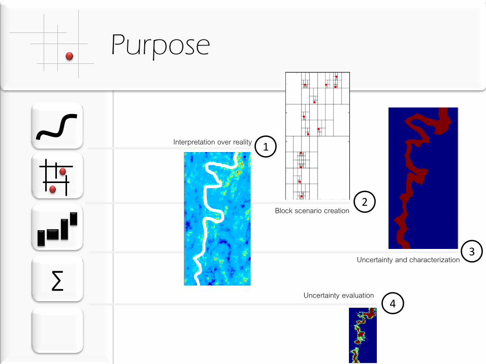
Block scenario creation

Uncertainty and characterization

Interpretation over reality

Uncertainty evaluation

1

2

3

4

Interpreting reality

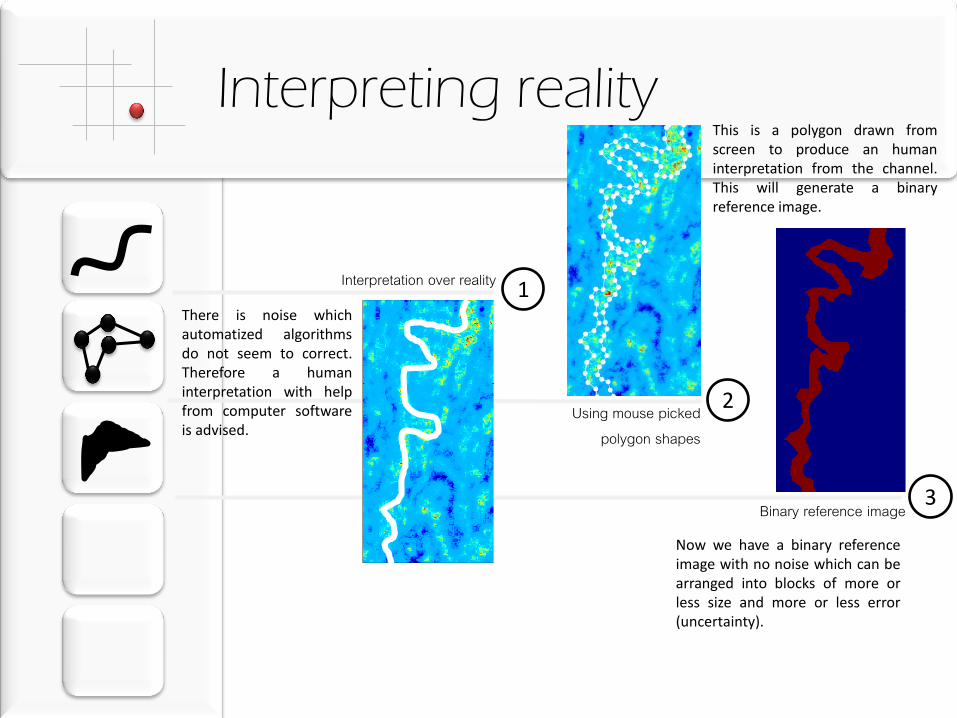
Interpretation over reality 1

There is noise which automatized algorithms do not seem to correct. Therefore a human interpretation with help from computer software is advised.

Using mouse picked polygon shapes

2

This is a polygon drawn from screen to produce an human interpretation from the channel. This will generate a binary reference image.

3 Binary reference image

Now we have a binary reference image with no noise which can be arranged into blocks of more or less size and more or less error (uncertainty).

What is a block?

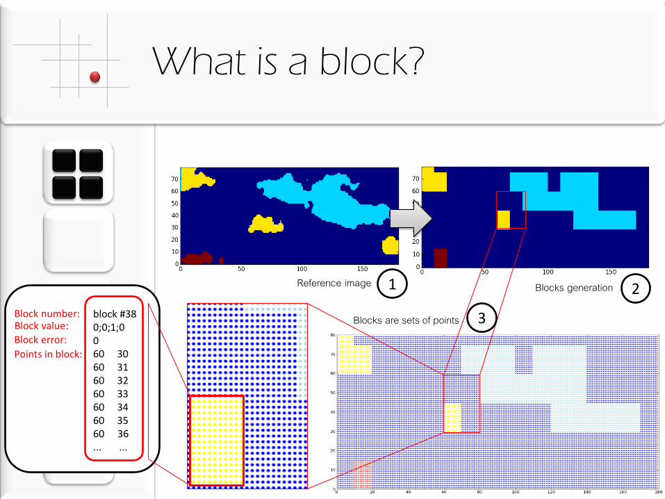
block #38 0;0;1;0 0 60 30 60 31 60 32 60 33 60 34 60 35 60 36 ... ...

Block number: Block value:

Block error:

Points in block:

1 2

3

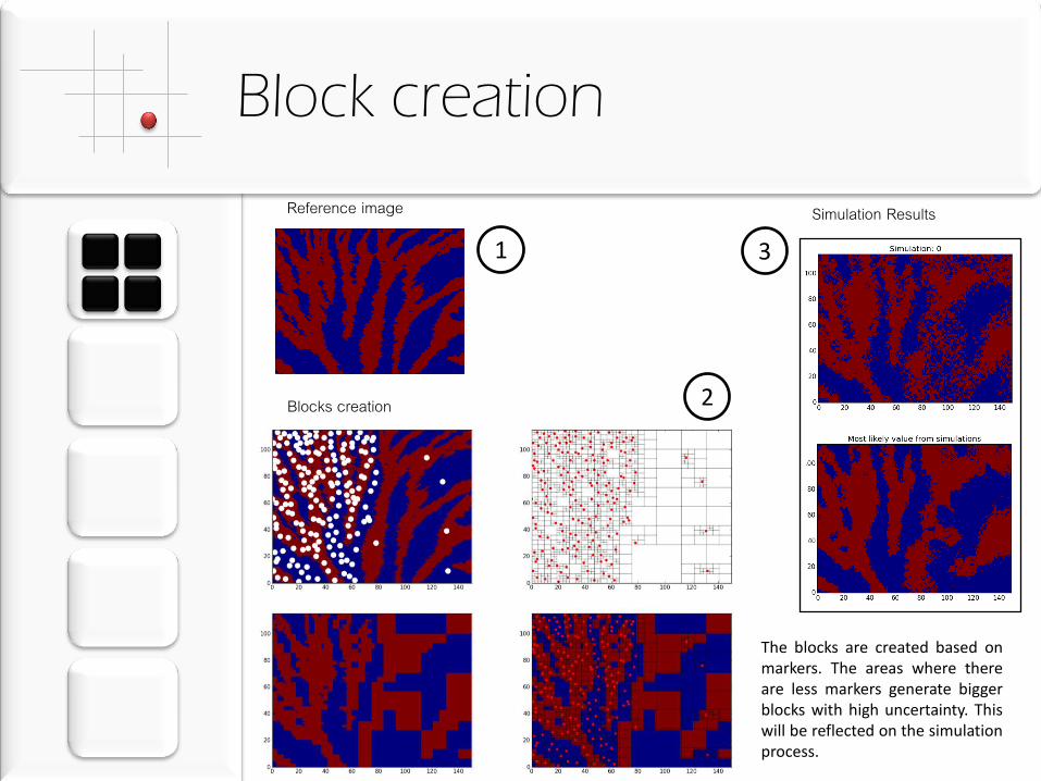
Reference image Blocks generation

Blocks are sets of points

Block creation

1

2

3

Reference image

Blocks creation

The blocks are created based on markers. The areas where there are less markers generate bigger blocks with high uncertainty. This will be reflected on the simulation process.

Simulation Results

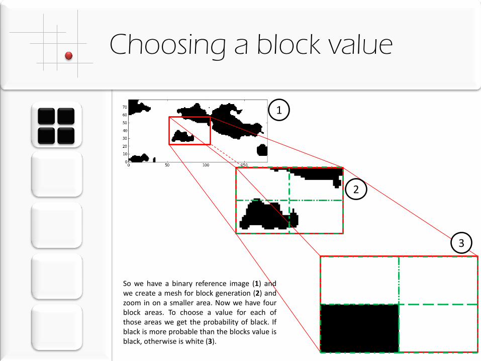
Choosing a block value

So we have a binary reference image (1) and we create a mesh for block generation (2) and zoom in on a smaller area. Now we have four block areas. To choose a value for each of those areas we get the probability of black. If black is more probable than the blocks value is black, otherwise is white (3).

1

2

3

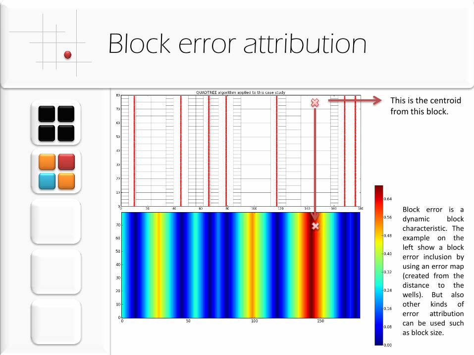
Block error attribution

This is the centroid from this block.

Block error is a dynamic block characteristic. The example on the left show a block error inclusion by using an error map (created from the distance to the wells). But also other kinds of error attribution can be used such as block size.

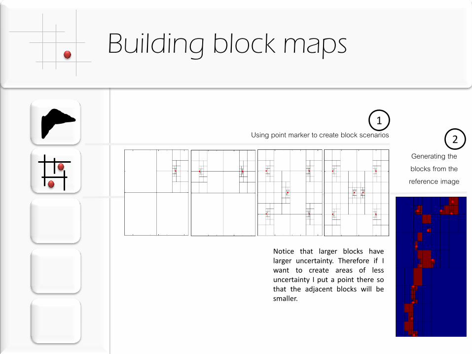
Building block maps

Using point marker to create block scenarios

Generating the blocks from the reference image

1

2

Notice that larger blocks have larger uncertainty. Therefore if I want to create areas of less uncertainty I put a point there so that the adjacent blocks will be smaller.

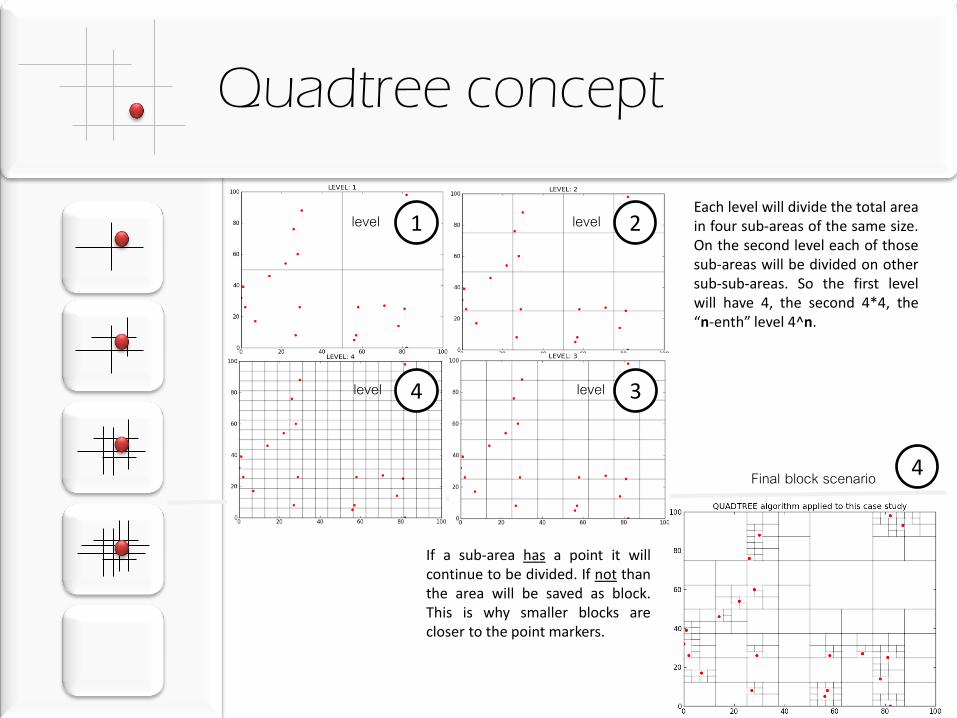
Quadtree concept

1 2

3 4

4 Final block scenario

level level

level level

Each level will divide the total area in four sub-areas of the same size. On the second level each of those sub-areas will be divided on other sub-sub-areas. So the first level will have 4, the second 4*4, the “n-enth” level 4^n.

If a sub-area has a point it will continue to be divided. If not than the area will be saved as block. This is why smaller blocks are closer to the point markers.

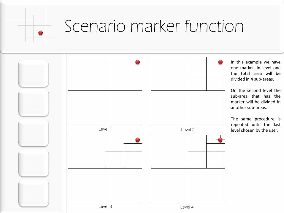
Scenario marker function

Level 1 Level 2

Level 3 Level 4

In this example we have one marker. In level one the total area will be divided in 4 sub-areas. On the second level the sub-area that has the marker will be divided in another sub-areas. The same procedure is repeated until the last level chosen by the user.

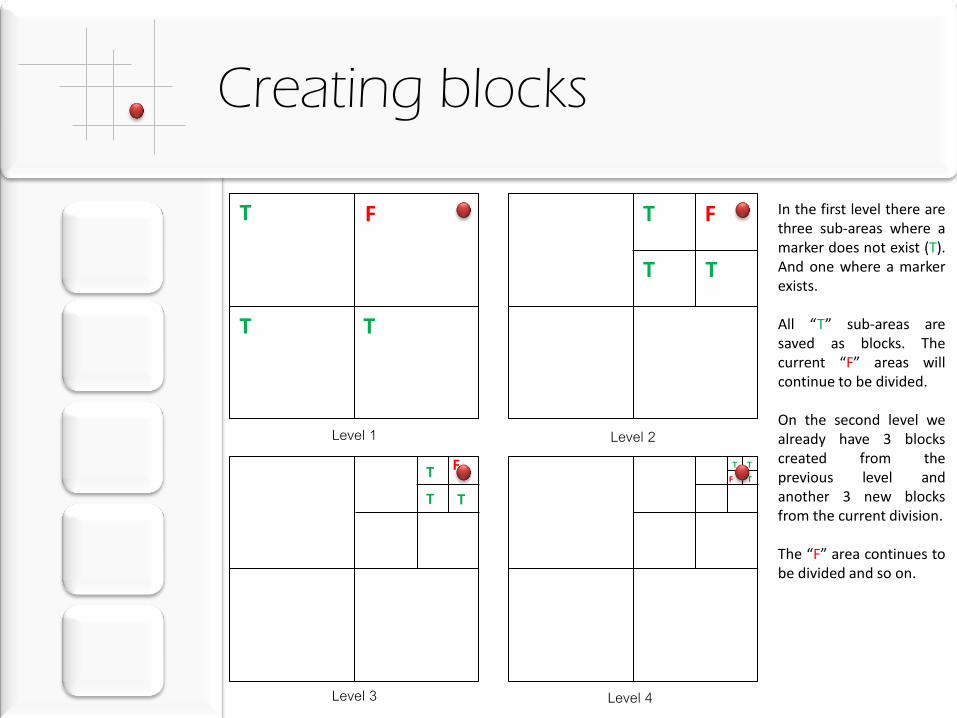
Creating blocks

T

T T

F T

T T

F

T

T T

F T T

T F

Level 1 Level 2

Level 3 Level 4

In the first level there are three sub-areas where a marker does not exist (T). And one where a marker exists. All “T” sub-areas are saved as blocks. The current “F” areas will continue to be divided. On the second level we already have 3 blocks created from the previous level and another 3 new blocks from the current division. The “F” area continues to be divided and so on.

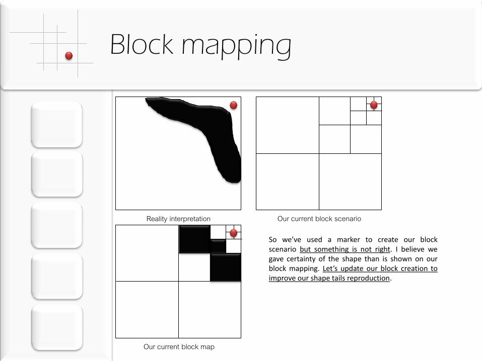
Block mapping

Our current block scenario Reality interpretation

Our current block map

So we’ve used a marker to create our block scenario but something is not right. I believe we gave certainty of the shape than is shown on our block mapping. Let’s update our block creation to improve our shape tails reproduction.

Updating for a better block

mapping

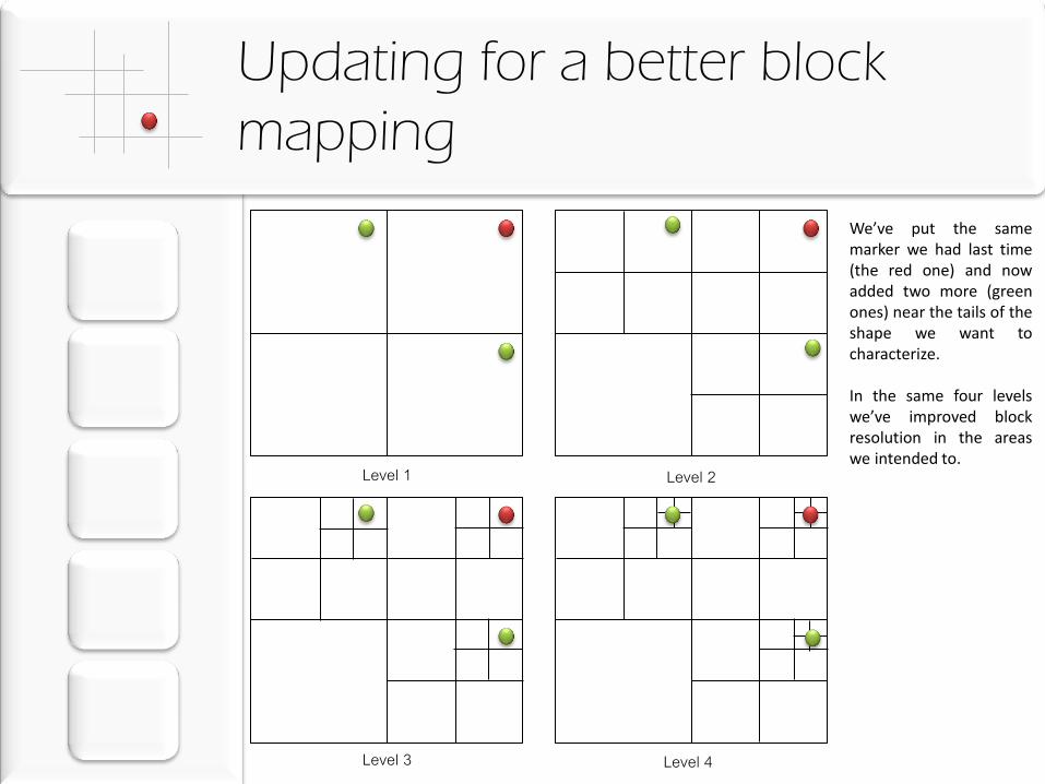
Level 1 Level 2

Level 3 Level 4

We’ve put the same marker we had last time (the red one) and now added two more (green ones) near the tails of the shape we want to characterize. In the same four levels we’ve improved block resolution in the areas we intended to.

Updating for a better block

mapping – Block creation

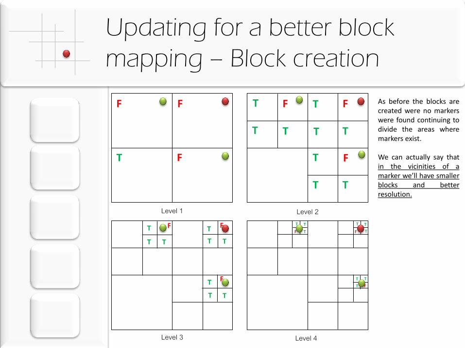
Level 1 Level 2

Level 3 Level 4

T

T

T T T

T

T

T

T T

F F

F

F F

F

T

T T

T

T T

T

T T

F F

F

T T

T

T T

T

T T

T

F F

F

As before the blocks are created were no markers were found continuing to divide the areas where markers exist. We can actually say that in the vicinities of a marker we’ll have smaller blocks and better resolution.

Updating for a better block

mapping – block mapping

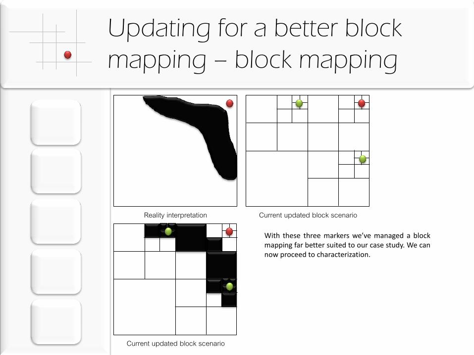
Current updated block scenario Reality interpretation

Current updated block scenario

With these three markers we’ve managed a block mapping far better suited to our case study. We can now proceed to characterization.

Uncertainty and characterization

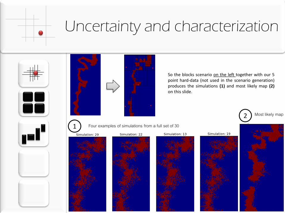
So the blocks scenario on the left together with our 5 point hard-data (not used in the scenario generation) produces the simulations (1) and most likely map (2) on this slide.

1 Four examples of simulations from a full set of 30

2 Most likely map

Uncertainty evaluation

1

2

3

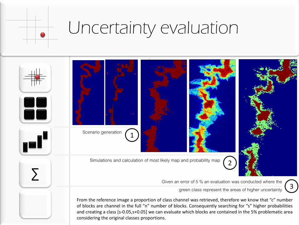
Scenario generation

Simulations and calculation of most likely map and probability map

Given an error of 5 % an evaluation was conducted where the green class represent the areas of higher uncertainty

∑

From the reference image a proportion of class channel was retrieved, therefore we know that “c” number of blocks are channel in the full “n” number of blocks. Consequently searching for “s” higher probabilities and creating a class [s-0.05,s+0.05] we can evaluate which blocks are contained in the 5% problematic area considering the original classes proportions.

Uncertainty evaluation

∑ 1

2 3

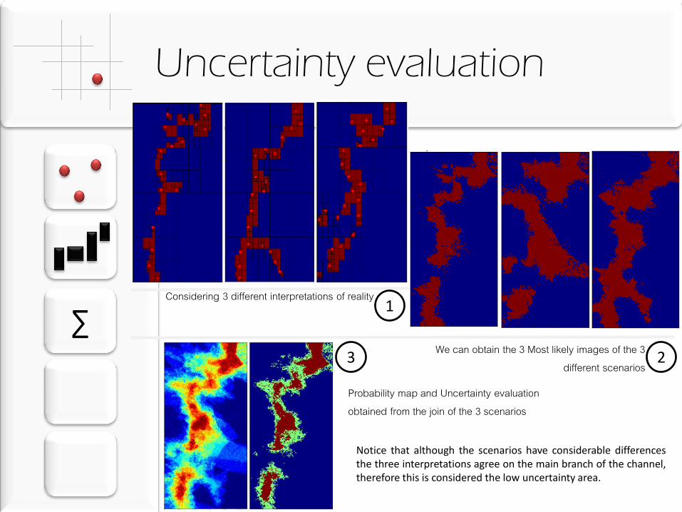
Considering 3 different interpretations of reality

We can obtain the 3 Most likely images of the 3 different scenarios

Probability map and Uncertainty evaluation obtained from the join of the 3 scenarios

Notice that although the scenarios have considerable differences the three interpretations agree on the main branch of the channel, therefore this is considered the low uncertainty area.

Uncertainty P10;P90

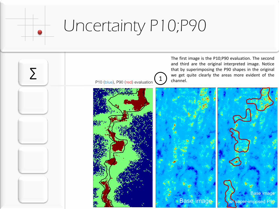
∑ P10 (blue), P90 (red) evaluation 1

Base image Base image

w/ super-imposed P90

The first image is the P10;P90 evaluation. The second and third are the original interpreted image. Notice that by superimposing the P90 shapes in the original we get quite clearly the areas more evident of the channel.

What is a block simulation?

1

2

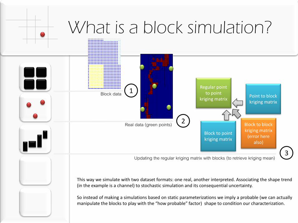
Block data

Real data (green points)

Regular point to point

kriging matrix Point to block kriging matrix

Block to point kriging matrix

Block to block kriging matrix

(error here also)

3 Updating the regular kriging matrix with blocks (to retrieve kriging mean)

This way we simulate with two dataset formats: one real, another interpreted. Associating the shape trend (in the example is a channel) to stochastic simulation and its consequential uncertainty. So instead of making a simulations based on static parameterizations we imply a probable (we can actually manipulate the blocks to play with the “how probable” factor) shape to condition our characterization.

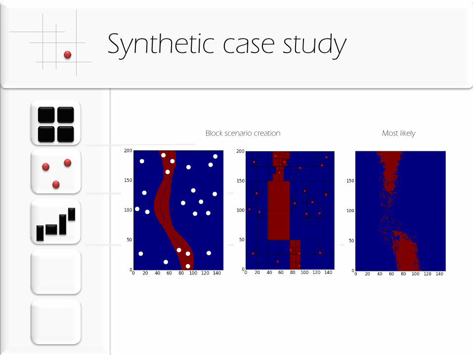
Synthetic case study

Block scenario creation Most likely

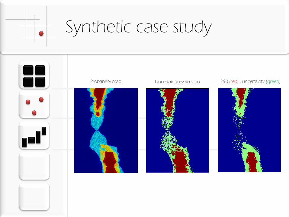
Synthetic case study

Probability map Uncertainty evaluation P90 (red) , uncertainty (green)

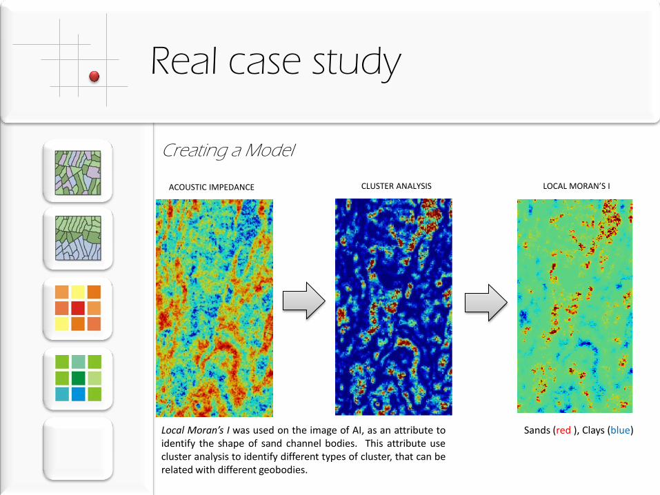
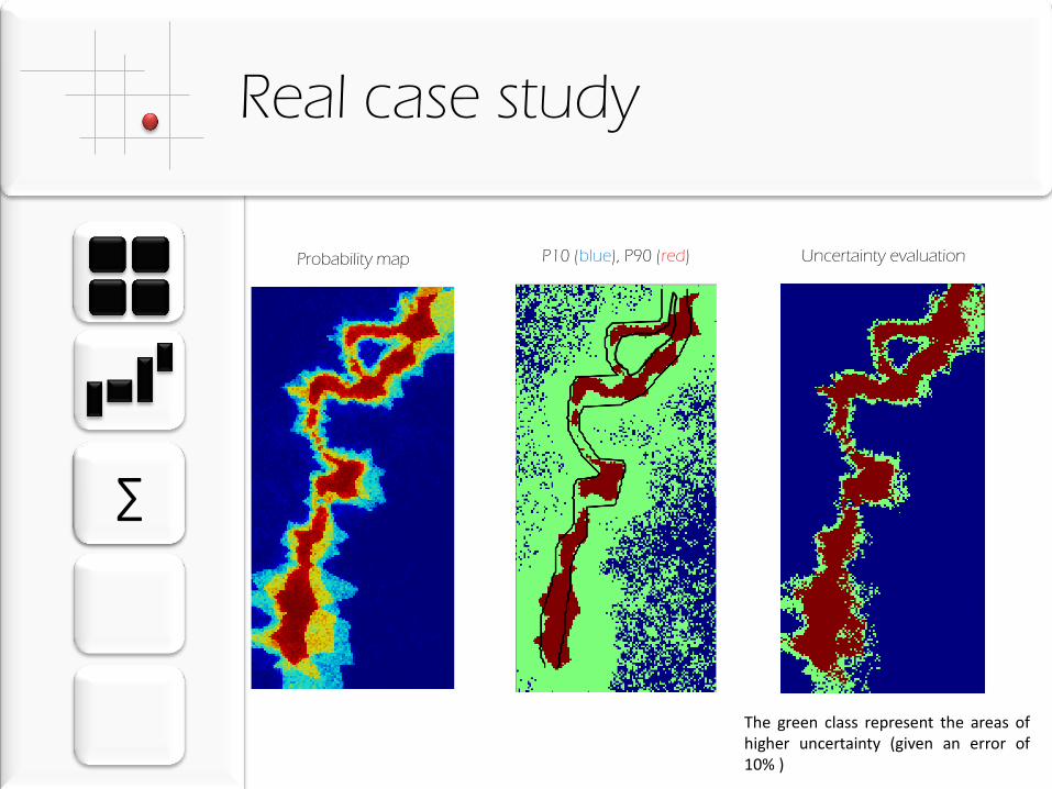
Real case study

ACOUSTIC IMPEDANCE CLUSTER ANALYSIS

Sands (red ), Clays (blue) Local Moran’s I was used on the image of AI, as an attribute to identify the shape of sand channel bodies. This attribute use cluster analysis to identify different types of cluster, that can be related with different geobodies.

Creating a Model

LOCAL MORAN’S I

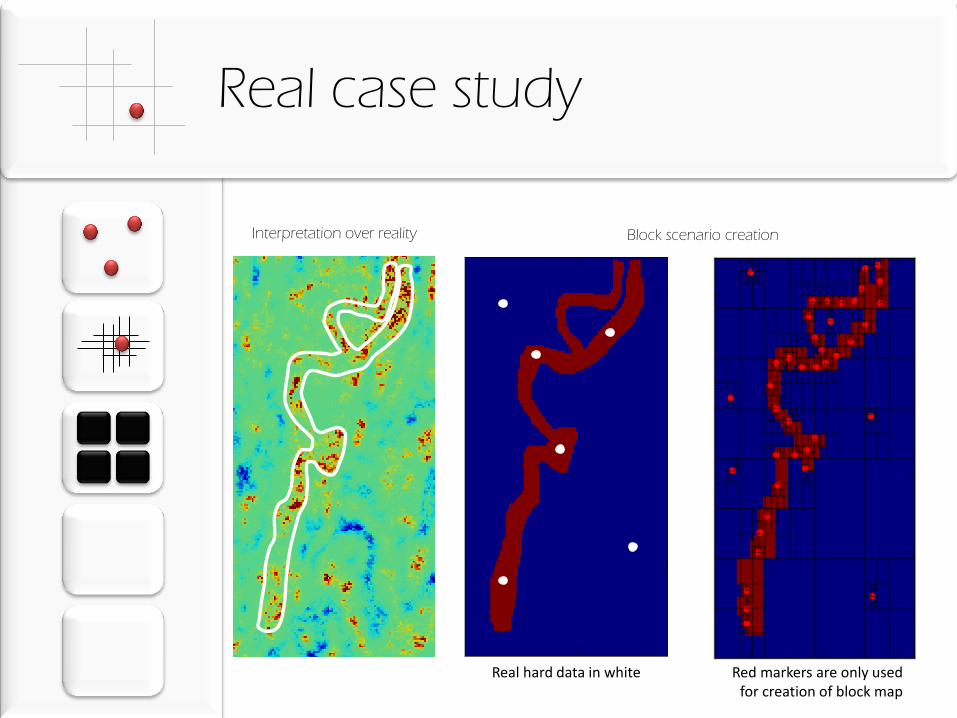
Real case study

Interpretation over reality Block scenario creation

Real hard data in white Red markers are only used for creation of block map

Real case study

∑

P10 (blue), P90 (red) Uncertainty evaluation Probability map

The green class represent the areas of higher uncertainty (given an error of 10% )