Shape ReconstructionUsing Active Tactile Sensors

Mark MollJuly 22, 2002CMU-CS-02-157

School of Computer ScienceCarnegie Mellon UniversityPittsburgh, PA 15213

Submitted in partial ful�llment of the requirementsfor the degree of Doctor of Philosophy.

Thesis Committee:Michael A. Erdmann, Chair

Kenneth Y. Goldberg, University of California, BerkeleyMatthew T. MasonAlfred A. Rizzi

Copyright © 2002, Mark Moll

This work was supported in part by the National Science Foundation under grant IIS-9820180

Keywords:Tactile sensing, shape reconstruction, nonprehensile manipulation,contact kinematics

Shape ReconstructionUsing Active Tactile Sensors

Mark Moll

AbstractWe present a new method to reconstruct the shape of an unknownobject using tactile sensors, without requiring object immobilization.Instead, sensing and nonprehensile manipulation occur simultane-ously. The robot infers the shape, motion and center of mass ofthe object based on the motion of the contact points as measuredby the tactile sensors. This allows for a natural, continuous inter-action between manipulation and sensing. We analyze the planarcase �rst by assuming quasistatic dynamics, and present simulationresults and experimental results obtained using this analysis. Weextend this analysis to the full dynamics and prove observability ofthe nonlinear system describing the shape and motion of the ob-ject being manipulated. In our simulations, a simple observer basedon Newton's method for root �nding can recover unknown shapeswith almost negligible errors. Using the same framework we canalso describe the shape and dynamics of three-dimensional objects.However, there are some fundamental di�erences between the planarand three-dimensional case, due to increased tangent dimensionality.Also, perfect global shape reconstruction is impossible in the 3D case,but it is almost trivial to obtain upper and lower bounds on the shape.The 3D shape reconstructionmethod has also been implemented andwe present some simulation results.

iii

A c k n o w l e d g m e n t s

First and foremost, I would like to thank the members of my thesis committeefor all their time and e�orts. I consider myself very lucky having had MichaelErdmann as my advisor. He has given me a tremendous amount of freedom inexploring di�erent directions. During our meetings he was always able to askthe right questions. Matt Mason has also been a great source of good ideas.Especially his intuitive mechanical insights have been really useful. Al Rizzi hasbeen very helpful in advising me on some control and engineering problems. KenGoldberg, my external committeemember, has givenme excellent feedback. I amalso grateful to him and Michael Erdmann for having given me the opportunityto work in Ken Goldberg's lab on a side project.Before coming to CarnegieMellon I have been fortunate to have worked with

two great researchers. I am greatly indebted toAntonNijholt, who has supportedme in many ways during my graduate studies at the University of Twente in theNetherlands and long afterward. I also enjoyed my collaboration with RistoMiikkulainen at the University of Texas in Austin. Through him I learned a lotabout doing research. He also encouraged me to pursue a PhD degree.Finally, I would like to thank members of the Manipulation Lab for their

support and brutal honesty during many of my lab presentations: Yan-Bin Jia,Garth Zeglin, Devin Balkcom, Siddartha Srinivasa, and Ravi Balasubramanian.Many thanks also to honorary Manipulation Lab member Howard Choset for hissupport and advice.

v

C o n t e n t s

Chapter 1 • Introduction 11.1 Motivation 11.2 Problem Statement 31.3 Thesis Outline 4

Chapter 2 • RelatedWork 72.1 Probing 72.2 Nonprehensile Manipulation 82.3 Grasping 112.4 Shape and Pose Recognition 122.5 Tactile Shape Reconstruction 132.6 Tactile Sensor Design 15

Chapter 3 • Quasistatic ShapeReconstruction 173.1 Notation 183.2 A Geometric Interpretation of Force/Torque Balance 233.3 Recovering Shape 253.4 Simulation Results 273.5 Experimental Results 333.6 Global Observability 353.7 Segmentation of Shape Reconstruction 43

Chapter 4 • Dynamic ShapeReconstruction 474.1 Equations of Motion 484.2 General Case 494.3 Moving the Palms at a Constant Rate 544.4 Fixed Palms 574.5 An Observer Based on Newton's Method 584.6 Simulation Results 604.7 Arbitrary Palm Shapes 63

vii

Chapter 5 • ShapeReconstruction in ThreeDimensions 675.1 Notation 675.2 Local Shape 705.3 Dynamics 745.4 Integrating Rotations 755.5 Simulation Results 765.6 Shape Approximations 79

Chapter 6 • Conclusion 836.1 Contributions 836.2 Future Directions 86

Appendix A • Derivations 93A.1 Quasistatic Shape Reconstruction 93A.2 Observability of the Planar Dynamic Case 96A.3 Force/Torque Balance in Three Dimensions 98

References 101

viii

L i s t o f F i g u r e s

1.1 Two possible arrangements of a smooth convex object resting on palms that arecovered with tactile sensors. 3

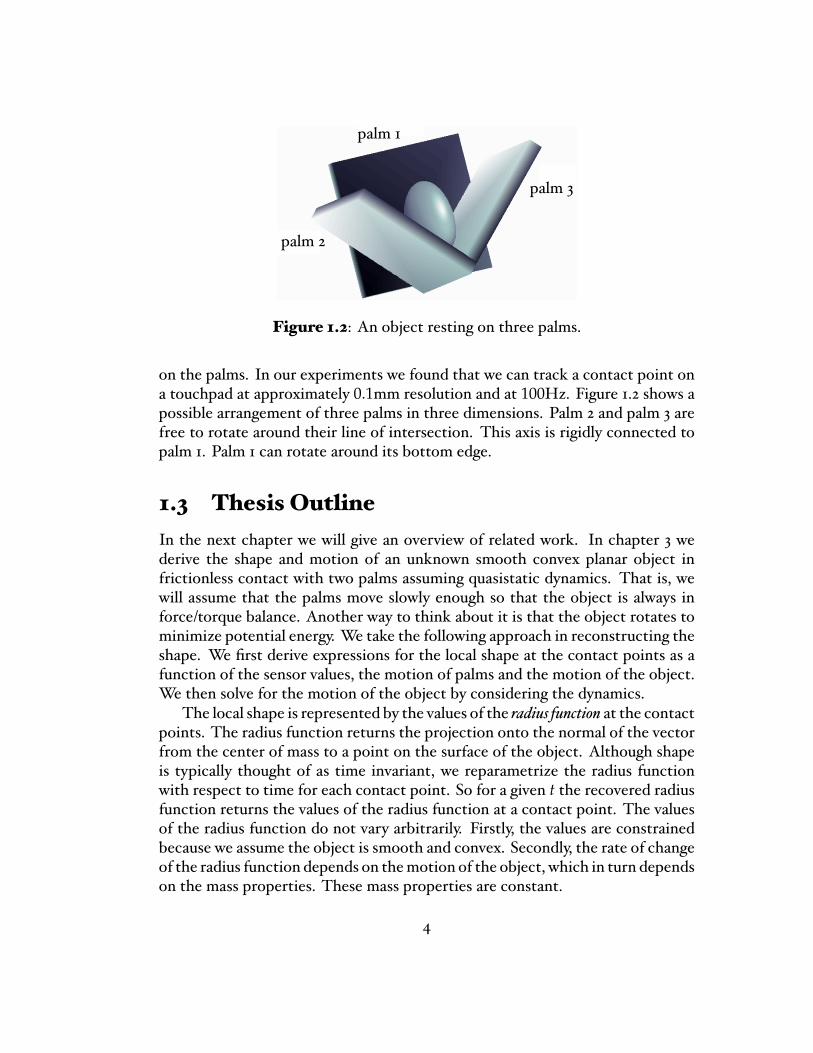
1.2 An object resting on three palms. 4

2.1 Related work in tactile shape reconstruction. 15

3.1 Inputs and outputs of the system formed by the palms and the object. 173.2 The contact support function. 183.3 The di�erent coordinate frames. 203.4 The generalized contact support functions. 213.5 The dependencies between sensor values, the support function and the angle

between the palms when the object makes two-point contact. 233.6 The frames show the reconstructed shape after 10, 20,. . . ,270 measurements. 293.7 The di�erences between the actual and observed shape. 303.8 The observable error for the reconstructed shape. 313.9 Resolution and sensing frequency of the VersaPad. 323.10 Setup of the palms. 333.11 Experimental setup. 343.12 Experimental results. 353.13 Stable poses for a particular shape. 363.14 Plan for observing the entire shape of an unknown object. 383.15 An antipodal grasp. 393.16 A more complicated stable pose surface. 403.17 Many stable poses are possible for a given palm con�guration that produce the

same sensor readings. 423.18 The error of two (radially) overlapping segments is equal to the area between

them. 44

4.1 Forces acting on the palms and the object. 484.2 Newton's method. 594.3 The frames show the reconstructed shape after 10, 20,. . . ,400 measurements. 614.4 Shape reconstruction with an observer based on Newton's method. 62

ix

4.5 Circular palms. 64

5.1 The coordinate frame de�ned using spherical coordinates 685.2 Illustration of the notation. 695.3 An object rolling and sliding on immobile palms with gravity and contact forces

acting on it. 785.4 Di�erences between real and recovered shape and motion. 795.5 The convex hull of the contact curves gives a lower bound on the volume

occupied by the object. 805.6 Two spherical palms holding an object. 81

6.1 Direction of the contact force in the absence and presence of friction. 866.2 Di�erent types of contact. 876.3 Dragging an object over a tactile sensor with a pivoting grasp. 906.4 A mobile robot consisting of two mass-less rods d1 and d2 connected at the

center of mass cm in contact with a curve. The wheels are at the end points ofd1 and d2. 91

x

N o t a t i o n

The notation in each chapter relies as much as possible on the notation used inprevious chapters. Below we only de�ne notation introduced in the correspond-ing chapter.

Chapter 3s1, s2 sensor values on palm 1 and palm 2, respectivelyφ1 angle between X-axis of the world frame and palm 1φ2 angle between palm 1 and palm 2φ0 orientation of the object held by the palmsR0 rotation matrix that maps points in the object's body coor-

dinates to world coordinatescm center of mass of the objectcr center of rotation of the objectx(θ) curve describing the shape of the objectv(θ) radius of curvature at x(θ)n(θ), t(θ) normal and tangent at x(θ)ni, ti normal and tangent at the contact point on palm i in world

coordinates(r(θ), d(θ)) contact support function(ri(θ), di(θ)) generalized contact support function relative to contact

point ie f error in force/torque balance constraintec error in two-point contact constraint

Chapter 4q vector describing the state of the system formed by the palms

and the objectFz the gravity vector acting on the objectg the gravity constant, equal to −9.81m/s2

Fci contact force at contact point i acting on the object

xi

fci magnitude of Fciτci torque generated by the contact force at contact point i on

the objectτi torque exerted by the motor of palm if (q) drift vector �eld; the rate of change of the system if no

torques are appliedgi(q) control vector �eld i; the rate of change of the system due to

τih(q) output function of the systemy output vector of the system; y = h(q)ωi, i = 0, 1, 2 rotational velocity of the object, palm 1, and palm 2αi, i = 0, 1, 2 angular acceleration of the object, palm 1, and palm 2a0 acceleration of the objectIi, i = 0, 1, 2 moment of inertia of the object, palm 1, and palm 2m mass of the objectρ radius of gyration of the objectdφ(q) di�erential of a function φ; dφ(q) =

( ∂φ∂q1

, . . . , ∂φ∂qn

)LXφ Lie derivative of a function φ along a vector �eld X; LXφ =

dφ · Xci contact point i in world coordinatesbi radius of circular palm iRi matrix describing the orientation of palm i

Chapter 5x(θ) surface describing the shape of the object[t1(θ),t2(θ),n(θ)] local coordinate frame at x(θ)(r(θ),d(θ),e(θ)) 3D contact support function[ti1,ti2,ni] coordinate frame at the contact point on palm i in world

coordinates.βi(t) curve in object coordinates traced out by contact point i on

the surface of the object.si = (si1, si2, 0)T vector of sensor values at palm iI inertia matrix of the objectφi angle between palm i and the horizontal plane

xii

C h a p t e r 1

Introduction

1.1 MotivationThere are many examples in everyday life of robotic systems that have almostnothing in common with the walking and talking humanoids of popular culture:robots assemble cars, assist in telesurgery, and can be used to assemble nano-structures. In all these examples it is critical that the robot can manipulate,sense, and reason about its environment. We can create a better understandingof fundamental manipulation and sensing strategies through rigorous explorationof the algorithmic and geometric aspects of robotics. For many tasks there is atrade-o� between manipulation and sensing. For example, a robot can establishthe orientation of an object with a vision system or by pushing and aligning theobject with a �xture. There is not only a trade-o�, but there are also interactionsbetween action and sensing. Sensor information can be used to guide certainactions, and manipulation can be used to reduce uncertainty about the state ofthe environment. There are many seemingly simple tasks such as tying shoelaces or recognizing an object by touching it, that pose enormous problems forautomated systems today. The di�culty of these tasks is caused in part by theuncertainty in the knowledge about the environment and by the di�culty oftightly integrating sensing with manipulation. In our research we aim to tightenthis integration as well as explore what the minimal manipulation and sensingrequirements are to perform a given task.Robotic manipulators typically cannot deal very well with objects of partially

unknown shape and weight. Humans, on the other hand, seem to have fewproblems with manipulating objects of unknown shape and weight. For example,Klatzky et al. (1985) showed that blindfolded human observers identi�ed 100common objects with over 96% accuracy, in only 1 to 2 seconds for most objects.Besides recognizing shape and size, humans also use touch to determine vari-

1

ous features such as texture, hardness, thermal qualities, weight and movement(Lederman and Browse, 1988).It seems unlikely that people mentally keep track of the exact position, shape

and mass properties of the objects in their environment. So somehow duringthe manipulation of an unknown object the tactile sensors in the human handgive enough information to �nd the pose and shape of that object. At the sametime some mass properties of the object are inferred to determine a good grasp.These observations are an important motivation for our research on tactile shapereconstruction. In most research on tactile shape reconstruction it is assumedthat the object being touched is in a �xture, or at least does not move as result ofbeing touched by a robot (Fearing and Binford, 1988; Montana, 1988; Allen andMichelman, 1990; Okamura and Cutkosky, 1999; Kaneko and Tsuji, 2001). Thismakes the shape reconstruction problem signi�cantly easier, but it introducesanother problem: how to immobilize an unknown object. In this thesis we donnot assume the object is immobilized. Instead, we will solve for the motionand shape of object simultaneously. In the process we will also recover themass properties of the object. We will show that the local shape and motionof an unknown object can be expressed as a function of the tactile sensor dataand the motion of the manipulators. By `local shape' we mean the shape atthe contact points. Our approach allows for a natural, continuous interactionbetween manipulation and sensing.As tactile sensors become more and more reliable and inexpensive, it seems

inevitable that touch sensors will be mounted on more general purpose robothands and manipulators. Being able to manipulate unknown objects is veryvaluable for robots that interact with the real world. It is often impossible topredict what the exact position of a robot and the exact forces should be tomanipulate an object. Being able to handle these uncertainties allows a robotto execute tasks that may only specify approximate descriptions of shape andposition of an object of interest. Pushing this idea even further, tactile datacan add another dimension to simultaneous localization and mapping (slam), animportant problem for mobile robots. But also in settings where the shapes andpositions of objects in the robot's workspace are known, tactile sensors couldprovide useful information. It is possible that there are slight variations in theshape and position of the objects, or that there are errors in the robot's position.With the information from tactile sensors the robot can adjust its position andre�ne its grasp. Tactile sensing may also be useful in manipulating deformableobjects. This would have applications in, e.g., medical robotics.We could also reconstruct an unknown shape with a camera by taking a series

of pictures and reconstruct the shape from that. However, recovering a shape

2

(a) Two palms.

φ1s1

XY

contact pt. 2

contact pt. 1

gravity‘palm’ 2

‘palm’ 1

O

φ2s2

(b) Two �ngers.

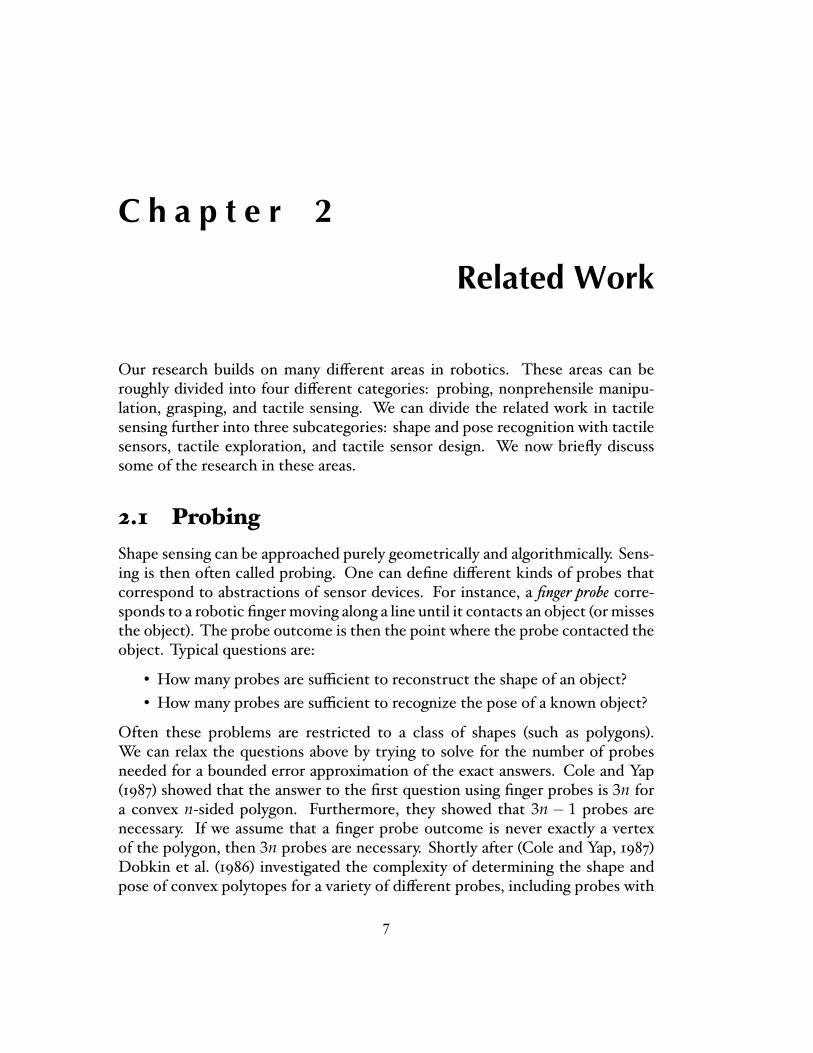
Figure 1.1: Two possible arrangements of a smooth convex object resting onpalms that are covered with tactile sensors.

from a series of images is not necessarily easier than recovering a shape from aset of curves traced out by the contact points. Often lighting and occlusion arebeyond control of the robot and make the reconstruction problem much harder.Also, from camera images it is not possible to infer mass properties of theunknown object. These mass properties are important if we want to manipulatethe object. As we will describe later in this thesis, it is possible to infer thesemass properties from tactile data. Of course, cameras and tactile sensors arenot mutually exclusive. Ideally, the information obtained from all sensors wouldbe combined to guide the robot. In this thesis we will focus exclusively on theinformation that can be extracted from tactile data.

1.2 ProblemStatementLet a palm be de�ned as a surface covered with tactile sensors. Suppose we have anunknown smooth convex object in contact with a number of moving palms (twopalms in two dimensions, three in three dimensions); the only forces acting onthe object are gravity and the contact forces. The curvature along the surface ofthe object is assumed to be strictly greater than zero, so that we have only onecontact point on each palm. For simplicity we assume that there is no friction.The central problem addressed in this thesis is the identi�cation of the mappingfrom the motion and sensor values of the palms to the local shape, motion, andmass properties of an unknown object.Figure 1.1 illustrates the basic idea. There are two palms that each have one

rotational degree of freedom at the point where they connect. That allows usto change the angle between palm 1 and palm 2 and between the palms and theglobal frame. As we change the palm angles we keep track of the contact pointsthrough tactile elements on the palms. We are using touchpads as tactile sensors

3

palm 2

palm 1

palm 3

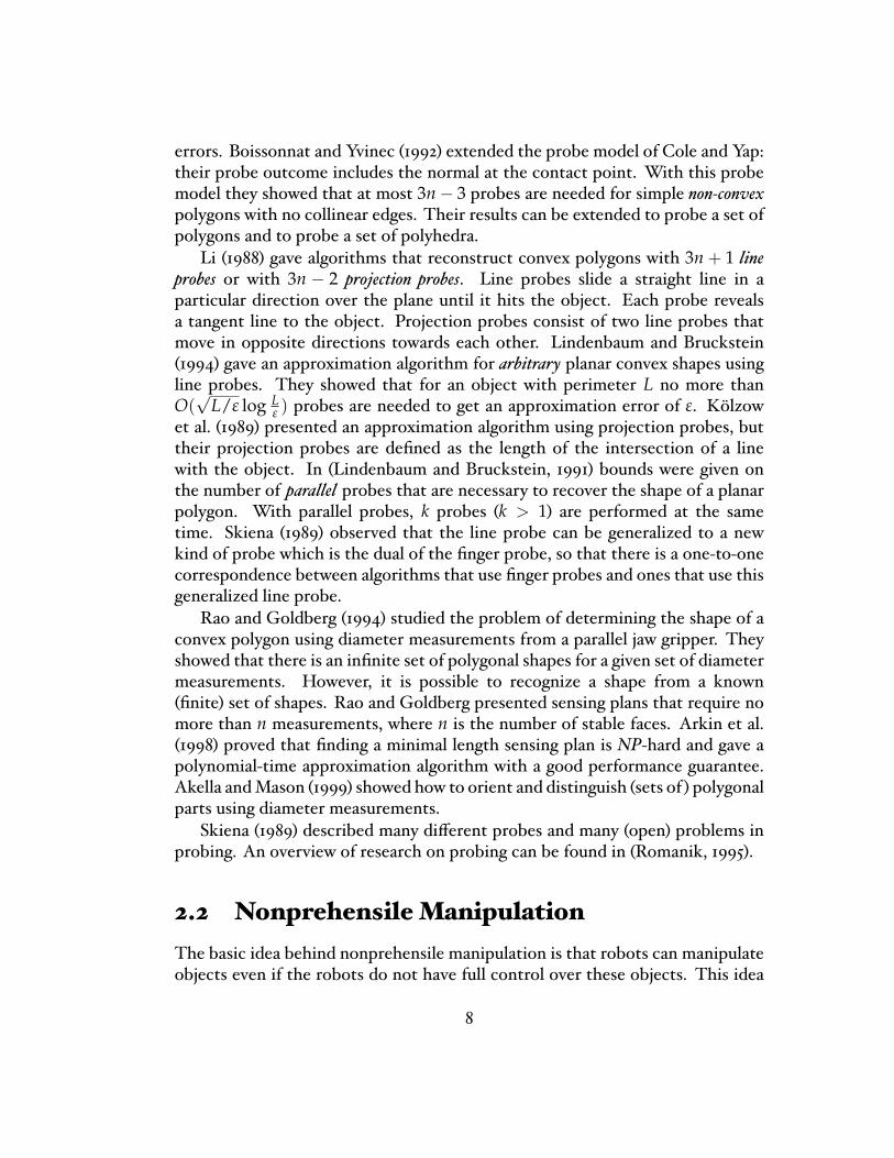
Figure 1.2: An object resting on three palms.

on the palms. In our experiments we found that we can track a contact point ona touchpad at approximately 0.1mm resolution and at 100Hz. Figure 1.2 shows apossible arrangement of three palms in three dimensions. Palm 2 and palm 3 arefree to rotate around their line of intersection. This axis is rigidly connected topalm 1. Palm 1 can rotate around its bottom edge.

1.3 Thesis OutlineIn the next chapter we will give an overview of related work. In chapter 3 wederive the shape and motion of an unknown smooth convex planar object infrictionless contact with two palms assuming quasistatic dynamics. That is, wewill assume that the palms move slowly enough so that the object is always inforce/torque balance. Another way to think about it is that the object rotates tominimize potential energy. We take the following approach in reconstructing theshape. We �rst derive expressions for the local shape at the contact points as afunction of the sensor values, the motion of palms and the motion of the object.We then solve for the motion of the object by considering the dynamics.The local shape is represented by the values of the radius function at the contact

points. The radius function returns the projection onto the normal of the vectorfrom the center of mass to a point on the surface of the object. Although shapeis typically thought of as time invariant, we reparametrize the radius functionwith respect to time for each contact point. So for a given t the recovered radiusfunction returns the values of the radius function at a contact point. The valuesof the radius function do not vary arbitrarily. Firstly, the values are constrainedbecause we assume the object is smooth and convex. Secondly, the rate of changeof the radius function depends on themotion of the object, which in turn dependson the mass properties. These mass properties are constant.

4

The solution for the shape andmotion of the object are in the formof a systemof di�erential equations, so the shape and motion of the object are obtained byintegration of these equations. We demonstrate the feasibility of this approachwith simulations and experimental results. We conjecture that, in general, it ispossible to reconstruct the entire shape. This may seem obvious, but it couldbe, for instance, that the robot can only reconstruct one side of the shape andthat it is impossible to reach the other side. To support this conjecture weanalyze the stable orientations in the con�guration space formed by the palmangles and object orientation. We show that the stable poses generally form aconnected surface, so that there exists a path between any orientation of theobject to any other orientation. The analysis of the stable pose surface givesrise to an open-loop manipulation strategy that has been used successfully insimulations. It is possible that the motion of the object has discontinuities, evenif the motion of the palms is continuous. This results in di�erent disconnectedor overlapping pieces of the shape. We will present a method for piecing thesedi�erent segments together.

In chapter 4 we will remove the quasistatic dynamics assumption. We willmodel the forces and torques exerted by the palms and by gravity. We can thensolve for the acceleration and angular acceleration of the object. By integratingtwice we can then obtain the position of the object at any given time. We willuse results from non-linear control theory to prove observability for the systemformed by the palms and the object. If a system is observable, then it is possibleto correct errors as time progresses. We �rst analyze the general case and thenconsider some special cases: (1) moving both palms at the same rate, (2) movingonly one palm, and (3) keeping both palms �xed. We prove that each case isobservable, but in the general case and in case 3 we rely on the e�ects of thecontrols to prove observability. There is no general method to construct anobserver for the general case and case 3. We did construct an observer for case 1and 2. With an observer it is possible to not only detect errors, but also drasticallyreduce errors in the state estimate. This means that if the estimate for the initialconditions for the system of di�erential equations is slightly wrong, an observerwill correct for that. More importantly, it �lters out noise and numerical errorthat might otherwise accumulate. The observer we implemented is based onNewton's method for �nding roots of a function. This observer works well insimulation.

Chapter 5 describes the generalization of the results in two dimensions tothree dimensions. The same approach carries over to 3D, but there are somefundamental di�erences. Most importantly, the contact points now trace outcurves on a surface, so it is impossible to create a complete reconstruction of

5

the shape in �nite time. We will show that these curves are less constrainedthan the contact point curves in 2D. This makes it impossible to construct anobserver within the current framework. Nevertheless, our simulations show thatgood results can still be obtained by integrating out the di�erential equationsthat describe the shape and motion of a 3D object. Although the system is notconstrained enough to prove observability, we have derived additional constraintsthat can be used to minimize an error measure. But since the system is notobservable, there is no guarantee that by minimizing this error measure the stateestimate converges to the true state.Finally, in chapter 6 we summarize the main contributions of this thesis and

outline di�erent future directions. Speci�cally, we describe how to remove someof the assumptions we made in this thesis. We also describe ways this work canbe extended to di�erent sensing modalities.

6

C h a p t e r 2

Related Work

Our research builds on many di�erent areas in robotics. These areas can beroughly divided into four di�erent categories: probing, nonprehensile manipu-lation, grasping, and tactile sensing. We can divide the related work in tactilesensing further into three subcategories: shape and pose recognition with tactilesensors, tactile exploration, and tactile sensor design. We now brie�y discusssome of the research in these areas.

2.1 ProbingShape sensing can be approached purely geometrically and algorithmically. Sens-ing is then often called probing. One can de�ne di�erent kinds of probes thatcorrespond to abstractions of sensor devices. For instance, a �nger probe corre-sponds to a robotic �ngermoving along a line until it contacts an object (ormissesthe object). The probe outcome is then the point where the probe contacted theobject. Typical questions are:

� How many probes are su�cient to reconstruct the shape of an object?� How many probes are su�cient to recognize the pose of a known object?

Often these problems are restricted to a class of shapes (such as polygons).We can relax the questions above by trying to solve for the number of probesneeded for a bounded error approximation of the exact answers. Cole and Yap(1987) showed that the answer to the �rst question using �nger probes is 3n fora convex n-sided polygon. Furthermore, they showed that 3n − 1 probes arenecessary. If we assume that a �nger probe outcome is never exactly a vertexof the polygon, then 3n probes are necessary. Shortly after (Cole and Yap, 1987)Dobkin et al. (1986) investigated the complexity of determining the shape andpose of convex polytopes for a variety of di�erent probes, including probes with

7

errors. Boissonnat and Yvinec (1992) extended the probe model of Cole and Yap:their probe outcome includes the normal at the contact point. With this probemodel they showed that at most 3n − 3 probes are needed for simple non-convexpolygons with no collinear edges. Their results can be extended to probe a set ofpolygons and to probe a set of polyhedra.Li (1988) gave algorithms that reconstruct convex polygons with 3n + 1 line

probes or with 3n − 2 projection probes. Line probes slide a straight line in aparticular direction over the plane until it hits the object. Each probe revealsa tangent line to the object. Projection probes consist of two line probes thatmove in opposite directions towards each other. Lindenbaum and Bruckstein(1994) gave an approximation algorithm for arbitrary planar convex shapes usingline probes. They showed that for an object with perimeter L no more thanO(√

L/ε log Lε ) probes are needed to get an approximation error of ε. Kölzow

et al. (1989) presented an approximation algorithm using projection probes, buttheir projection probes are de�ned as the length of the intersection of a linewith the object. In (Lindenbaum and Bruckstein, 1991) bounds were given onthe number of parallel probes that are necessary to recover the shape of a planarpolygon. With parallel probes, k probes (k > 1) are performed at the sametime. Skiena (1989) observed that the line probe can be generalized to a newkind of probe which is the dual of the �nger probe, so that there is a one-to-onecorrespondence between algorithms that use �nger probes and ones that use thisgeneralized line probe.Rao and Goldberg (1994) studied the problem of determining the shape of a

convex polygon using diameter measurements from a parallel jaw gripper. Theyshowed that there is an in�nite set of polygonal shapes for a given set of diametermeasurements. However, it is possible to recognize a shape from a known(�nite) set of shapes. Rao and Goldberg presented sensing plans that require nomore than n measurements, where n is the number of stable faces. Arkin et al.(1998) proved that �nding a minimal length sensing plan is NP-hard and gave apolynomial-time approximation algorithm with a good performance guarantee.Akella andMason (1999) showed how to orient and distinguish (sets of ) polygonalparts using diameter measurements.Skiena (1989) described many di�erent probes and many (open) problems in

probing. An overview of research on probing can be found in (Romanik, 1995).

2.2 NonprehensileManipulationThe basic idea behind nonprehensile manipulation is that robots can manipulateobjects even if the robots do not have full control over these objects. This idea

8

was pioneered by Mason. In his Ph.D. thesis (Mason, 1982) and the companionpaper (Mason, 1985) nonprehensile manipulation took the form of pushing anobject in the plane to reduce uncertainty about the object's pose. Further workby Peshkin and colleagues (Peshkin and Sanderson, 1988; Wiegley et al., 1996)analyzed the pushing problem and showed how to design fences for a conveyorbelt system. Berretty et al. (1998) proved the conjecture of Wiegley et al. (1996)that any polygonal part can be oriented by a sequence of fences and presentedan O(n3 log n) algorithm to compute the shortest such sequence. The workon fence design has recently been generalized to polyhedral objects by Berretty(2000). Berretty described a system where parts were fed from one conveyor beltto another, each belt with a sequence of fences. Akella et al. (2000) described asystemwhere a sequence of fences was replaced with a one joint robot. The robotwas basically a movable fence with one rotational degree of freedom. The robotcould push a part up a conveyor belt and let it drift back. Akella et al. presented analgorithm that �nds a sequence of pushes to orient a given polygonal part withoutsensing. Lynch (1997) further built on Mason's work. In his Ph.D. thesis Lynchdescribed a path planner for quasistatically pushing objects among obstacles. Healso investigated controllability of dynamic nonprehensile manipulation such asthrowing and catching a part. Lynch et al. (1998) showed how to make a roboticmanipulator perform a certain juggling motion with a suitable parameterizationof the shape and motion of the manipulator. Much research on juggling balls hasbeen done in Koditschek's research group (see e.g. (Rizzi and Koditschek, 1993)and (Whitcomb et al., 1993)). Rizzi and Koditschek (1993) described a systemconsisting of a robot arm and a camera that can juggle two balls. In (Abell andErdmann, 1995) nonprehensile manipulation took the (abstract) form of movingtwo frictionless contacts on a polygonal part in a planar gravitational �eld. Abelland Erdmann presented an algorithm to orient such a polygonal part by movingthe contact points and performing hand-o�s between two pairs of contact points.

Erdmann and Mason (1988) described sensorless manipulation within theformal framework of the preimage methodology (Lozano-Pérez et al., 1984). Inparticular, Erdmann and Mason showed how to orient a planar object by a traytilting device: �rst, the object is placed in a randomunknown pose in the tray and,second, the tray is tilted at a sequence of angles to bring the object in a uniquepose. In (Erdmann et al., 1993) the tray tilting idea was extended to polyhedra.

The pushing and tilting primitives can be formulated as parametrized func-tions that map orientations to orientations. The parameters of such a functionare then the push direction and the tilt angle, respectively. By composing thesefunctions one can orient a part without sensing. Eppstein (1990) presented a verygeneral algorithm that takes a set of functions as input. Given these functions

9

the algorithm computes a shortest sequence of these functions that will orient apolygonal part. Goldberg (1993) introduced another primitive: squeezing with aparallel-jaw gripper. By making one jaw compliant in the tangential direction, thecontacts with the part are e�ectively frictionless. Goldberg proved that for everyn-sided polygonal part, a sequence of `squeezes' can be computed in O(n2 log n)time that will orient the part up to symmetry. The length of such a sequenceis bounded by O(n2). Chen and Ierardi (1995) improved this bound to O(n)and showed that the algorithm runs in O(n2). (Van der Stappen et al., 2000)presented improved bounds that depend on the geometric eccentricity (intuitively,how �fat� or �thin� a part is). Their analysis also applies to curved parts. Recently,Moll et al. (2002) introduced a new primitive for orientingmicro-scale parts usinga parallel jaw gripper. Moll et al. showed that any polygonal part can be orientedwith a sequence of rollingmotions, where the part is rolled between the two jaws.With this primitive the gripper does not need to be reoriented.One of the �rst papers in palmar manipulation is (Salisbury, 1987). Salisbury

suggested a new approach to manipulation in which the whole robot arm is usedas opposed to just the �ngertips. Paljug et al. (1994) investigated the problemof multi-arm manipulation. Paljug et al. presented a nonlinear feedback schemefor simultaneous control of the trajectory of the object being manipulated aswell as the contact conditions. Erdmann (1998) showed how to manipulate aknown object with two palms. He also presented methods for determining thecontact modes of each palm: rolling, sliding and holding the object. Zumel (1997)described a palmar system like the one shown in �gure 1.1(b), but without tactilesensors. Zumel derived su�cient conditions for orienting known polygonal partswith these palms. She also showed that an orienting plan for a polygon can becomputed inO(N2) and that the length isO(N), where N is the number of stableedges of the polygon.Another way to orient parts is to design a manipulator shape speci�cally for

a given part. This approach was �rst considered for the Sony APOS system(Hitakawa, 1988). The design was done mainly by ad-hoc trial and error. Later,Moll and Erdmann (2002) explored a way to automate this process.In recent years a lot of work has been done on programmable force �elds to

orient parts (Böhringer et al., 2000a, 1999; Kavraki, 1997; Reznik et al., 1999)The idea is that an abstract force �eld (implemented using e.g. MEMS actuatorarrays) can be used to push the part into a certain orientation. Böhringer et al.used Goldberg's algorithm (1993) to de�ne a sequence of `squeeze �elds' to orienta part. They also gave an example how programmable vector �elds can be usedto simultaneously sort di�erent parts and orient them. Kavraki (1997) presenteda vector �eld that induced two stable con�gurations for most parts. In 2000,

10

Böhringer et al. proved a long-standing conjecture that the vector �eld proposedin (Böhringer et al., 1996) is a universal feeder/orienter device, i.e., it induces aunique stable con�guration for most parts. Recently, Sudsang and Kavraki (2001)introduced another vector �eld that has the universal feeder property.

2.3 GraspingThe problem of grasping has been widely studied. This section will not try togive a complete overview of the results in this area, but instead just mentionsome of the work that is most important to our problem. Much of the graspresearch focuses on computing grasps that establish force-closure (the ability toresist external forces) and form-closure (a kinematic constraint condition thatprevents all motion). Important work includes (Salisbury, 1982), (Cutkosky,1985), (Fearing, 1984), (Kerr and Roth, 1986), (Mishra et al., 1987), (Montana,1988), (Nguyen, 1988), (Trinkle et al., 1988), (Hong et al., 1990), (Markensco� et al.,1990), and (Ponce et al., 1997). For an overview of grasp synthesis algorithms seee.g. (Shimoga, 1996).To grasp an object one needs to understand the kinematics of contact. Inde-

pendently, Montana (1988) and Cai and Roth (1986, 1987) derived the relationshipbetween the relativemotion of two objects and themotion of their contact point.In (Montana, 1995) these results were extended to multi-�ngered manipulation.Sudsang et al. (2000) looked at theproblemofmanipulating three-dimensional

objects with a recon�gurable gripper. The gripper consisted of two horizontalplates, of which the top one had a regular grid of actuated pins. They presenteda planner that computed a sequence of pin con�gurations that brought an objectfrom one con�guration to another using so-called immobility regions. For each(intermediate) con�guration only three pins were needed. Plans were restrictedto ones where the object maintains the same set of contact points with the bot-tom plate. Rao et al. (1994, 1995) showed how to reorient a polyhedral objectwith pivoting grasps: the object was grasped with two hard �nger contacts so thatit pivoted under gravity when lifted. Often only one pivot grasp was su�cient tobring the object from one stable pose to another (provided the friction coe�cientwas large enough).Trinkle and colleagues (Trinkle et al., 1993; Trinkle and Hunter, 1991; Trinkle

and Paul, 1990; Trinkle et al., 1988) investigated the problem of dexterous ma-nipulation with frictionless contact. They analyzed the problem of lifting andmanipulating an object with enveloping grasps. Kao and Cutkosky (1992) andYoshikawa et al. (1993) did not assume frictionless contacts. Whereas Kao andCutkosky focused on modeling sliding contact with compliance, Yoshikawa et al.

11

showed how to regrasp an object using quasistatic slip motion. Nagata et al.(1993) described a method of repeatedly regrasping an object to build up a modelof its shape.Grupen and Coelho Jr. (1993; 1996) proposed an on-line grasp synthesis

method for a robot hand equipped with sensors. The controllers of the handused sensor data to re�ne a grasp. Teichmann and Mishra (2000) presented analgorithm that determines a good grasp for an unknown object using a parallel-jaw gripper equipped with light beam sensors. This paper also presented a tightintegration of sensing andmanipulation. Interestingly, the object is not disturbeduntil good grasp points are found.Erdmann (1995) proposed a method for automatically designing sensors from

the speci�cation of the robot's task. Erdmann gives the example of graspingan ellipse. By sensing some aspect of the local geometry at the contact points,it is possible to de�ne a feedback loop that guides the �ngers toward a stablegrasp. Recently, Jia (2000) extended these results and showed how to achieve anantipodal grasp of a curved planar object with two �ngers. By rolling the �ngersaround the object the pose of the object is determined and then the �ngers arerolled to two antipodal points.

2.4 Shape and Pose RecognitionThe problem of shape and pose recognition can be stated as follows: suppose wehave a known set of objects, how can we recognize one of the objects if it is inan unknown pose? For an in�nite set of objects the problem is often phrased as:suppose we have a class of parametrized shapes, can we establish the parametersfor an object from that class in an unknown pose? Schneiter and Sheridan (1990)and Ellis (1992) developed methods for determining sensor paths to solve the �rstproblem. In Siegel (1991) a di�erent approach is taken: the pose of an object isdetermined by using an enveloping grasp. This method uses only joint angle andtorque sensing.Grimson and Lozano-Pérez (1984) used measurements of positions and sur-

face normals to recognize and locate objects from among a set of known polyhe-dral objects. They phrased the recognition problem as a constraint satisfactionproblem using an interpretation tree. Interpretation trees were introduced byGaston and Lozano-Pérez (1984) as a way to match sets of contact points withedges of an object.Kang and Goldberg (1995) used a Bayesian approach to recognizing arbitrary

planar parts from a known set. Their approach consists of randomly graspinga part with a parallel-jaw gripper. Each grasp returns a diameter measurement,

12

which can be used to update a probability for each part in the set of known parts.Using a statistical measure of similarity it is possible to predict the expectednumber of grasps to recognize a part.Jia and Erdmann (1996) proposed another `probing-style' solution: they de-

termined possible poses for polygons from a �nite set of possible poses. Onecan think of this �nite set as the stable poses (for some sense of stable). Onemethod determines the pose by bounding the polygon by supporting lines. Thesecond method they propose is to sense by point sampling. They prove that solv-ing this problem is NP-complete and present a polynomial time approximationalgorithm.Keren et al. (1998) proposed a method for recognizing three-dimensional

objects using curve invariants. This idea was motivated by the fact that tactilesensor data often takes the form of a curve on the object. They apply theirmethod to geometric primitives like spheres and cylinders.Jia and Erdmann (1999) investigated the problem of determining not only the

pose, but also the motion of a known object. The motion of the object is inducedby having a robotic �nger push the object. By tracking the contact point on the�nger, they were able to recover the pose and motion using nonlinear observertheory.

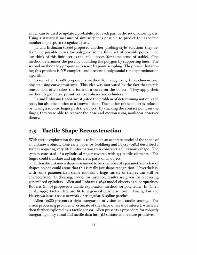
2.5 Tactile ShapeReconstructionWith tactile exploration the goal is to build up an accurate model of the shape ofan unknown object. One early paper by Goldberg and Bajcsy (1984) described asystem requiring very little information to reconstruct an unknown shape. Thesystem consisted of a cylindrical �nger covered with 133 tactile elements. The�nger could translate and tap di�erent parts of an object.Often the unknown shape is assumed tobe amember of a parametrized class of

shapes, so one could argue that this is really just shape recognition. Nevertheless,with some parametrized shape models, a large variety of shapes can still becharacterized. In (Fearing, 1990), for instance, results are given for recoveringgeneralized cylinders. Allen and Roberts (1989) model objects as superquadrics.Roberts (1990) proposed a tactile exploration method for polyhedra. In (Chenet al., 1996) tactile data are �t to a general quadratic form. Finally, Liu andHasegawa (2001) use a network of triangular B-spline patches.Allen (1988) presents a tight integration of vision and tactile sensing. The

vision processing provides an estimate of the shape of areas of interest, which arethen further explored by a tactile sensor. Allen presents a procedure for robustlyintegrating noisy visual and tactile data into 3D surface and feature primitives.

13

Allen andMichelman (1990) presented methods for exploring shapes in threestages, from coarse to �ne: grasping by containment, planar surface exploringand surface contour following. Montana (1988) described a method to estimatecurvature based on a number of probes. Montana also presented a control law forcontour following. Charlebois et al. (1996, 1997) introduced two di�erent tactileexploration methods. The �rst method is based on rolling a �nger around theobject to estimate the curvature using Montana's contact equations. Charleboiset al. analyze the sensitivity of this method to noise. With the second methoda B-spline surface is �tted to the contact points and normals obtained by slidingmultiple �ngers along an unknown object.Marigo et al. (1997) showed how to manipulate a known polyhedral part by

rolling it between the two palms of a parallel-jaw gripper. Bicchi et al. (1999)extended these results to tactile exploration of unknown objects with a parallel-jaw gripper equipped with tactile sensors. The two palms of the gripper rollthe object without slipping and track the contact points. Using tools fromregularization theory they produce spline-like models that best �t the sensordata. The work by Bicchi and colleagues is di�erent from most other work ontactile shape reconstruction in that the object being sensed is not immobilized.With our approach the object is not immobilized either, but whereas Bicchi andcolleagues assumed pure rolling we assume pure sliding.A di�erent approach is taken by Kaneko and Tsuji (2001), who try to recover

the shape by pulling a �nger over the surface. With this �nger they can also probeconcavities. In (Okamura and Cutkosky, 1999; Okamura et al., 1999; Okamuraand Cutkosky, 2001) the emphasis is on detecting �ne surface features such asbumps and ridges. Sensing is done by rolling a �nger around the object. (Okamuraet al., 1999) show how one can measure friction by dragging a block over a surfaceat di�erent velocities, measure the forces and solve for the unknowns. Thiswork builds forth on previous work by Cutkosky and Hyde (1993), who proposean event-driven approach to dextrous manipulation. During manipulation ofan object there are several events that can be detected with tactile sensing.Examples of such events are: making and breaking contact, slipping, change infriction, texture, sti�ness, etc. Based on these events it is possible to infer someof the object's properties (such as its shape and mass distribution) and adjust thegrasp.Much of our work builds forth on (Erdmann, 1999). There, the shape of planar

objects is recognized by three palms; two palms are at a �xed angle, the thirdpalm can translate compliantly, ensuring that the object touches all three palms.Erdmann derives the shape of an unknown object with an unknown motion as afunction of the sensor values. In our work we no longer assume that the motion

14

tactile shape reconstruction

������

���

HHHHHH

HHH

immobilizedobjects

Fearing, Montana,Allen &Michelman,Okamura & Cutkosky,Kaneko & Tsuji

moving objects

�����

HHHHH

pure rollingBicchi, Marigo et al.

pure slidingErdmann,Moll

Figure 2.1: Related work in tactile shape reconstruction.

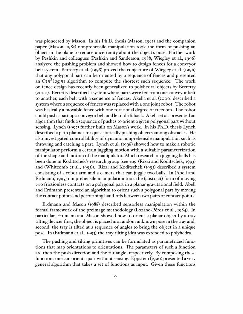
of the object is completely arbitrary. Instead, we model the dynamics of theobject as it is manipulated by the palms. Only gravity and the contact forces areacting on the object. As a result we can recover the shape with fewer sensors.By modeling the dynamics we need one palm less in 2D. In the 3D case, insteadof six palms, we need only three. Figure 2.1 shows where our research �ts withinthe �eld of tactile shape reconstruction. In the long term we plan to develop auni�ed framework for reconstructing the shape and motion of unknown objectwith varying contact modes.

2.6 Tactile SensorDesignDespite the large body of work in tactile sensing and haptics, making reliable andaccurate tactile sensors has proven to be very hard. Many di�erent designs havebeen proposed. This section will mention just a few. For an overview of sensingtechnologies, see e.g. (Lee, 2000), (Howe and Cutkosky, 1992) and (Nicholls andLee, 1989). Fearing and Binford (1988) describe a cylindrical tactile sensor todetermine the curvature of convex unknown shapes. Russell (1992) introducesso-called whisker sensors: curved rods, whose de�ection is measured with apotentiometer. Kaneko and Tsuji (2001) have developed planning algorithms torecover the shape of an object with such whiskers. Speeter (1990) describes atactile sensing system consisting of up to 16 arrays of 256 tactile elements thatcan be accessed in parallel. He discusses the implementation issues involved

15

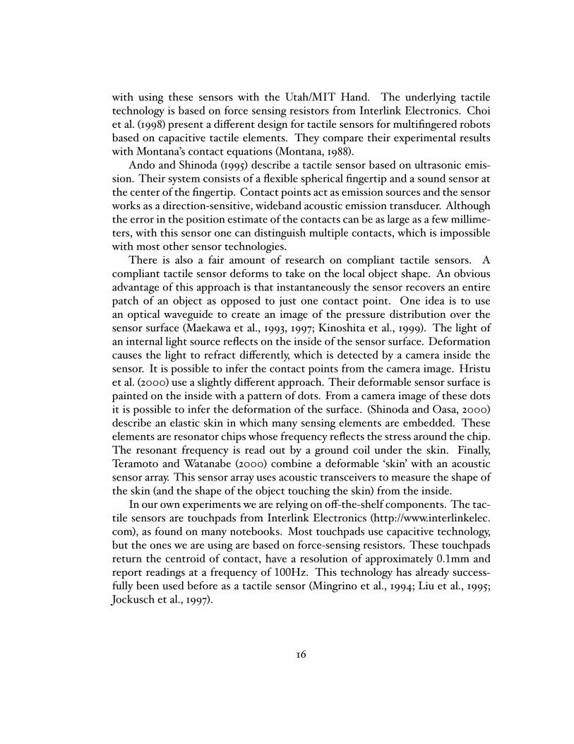
with using these sensors with the Utah/MIT Hand. The underlying tactiletechnology is based on force sensing resistors from Interlink Electronics. Choiet al. (1998) present a di�erent design for tactile sensors for multi�ngered robotsbased on capacitive tactile elements. They compare their experimental resultswith Montana's contact equations (Montana, 1988).Ando and Shinoda (1995) describe a tactile sensor based on ultrasonic emis-

sion. Their system consists of a �exible spherical �ngertip and a sound sensor atthe center of the �ngertip. Contact points act as emission sources and the sensorworks as a direction-sensitive, wideband acoustic emission transducer. Althoughthe error in the position estimate of the contacts can be as large as a few millime-ters, with this sensor one can distinguish multiple contacts, which is impossiblewith most other sensor technologies.There is also a fair amount of research on compliant tactile sensors. A

compliant tactile sensor deforms to take on the local object shape. An obviousadvantage of this approach is that instantaneously the sensor recovers an entirepatch of an object as opposed to just one contact point. One idea is to usean optical waveguide to create an image of the pressure distribution over thesensor surface (Maekawa et al., 1993, 1997; Kinoshita et al., 1999). The light ofan internal light source re�ects on the inside of the sensor surface. Deformationcauses the light to refract di�erently, which is detected by a camera inside thesensor. It is possible to infer the contact points from the camera image. Hristuet al. (2000) use a slightly di�erent approach. Their deformable sensor surface ispainted on the inside with a pattern of dots. From a camera image of these dotsit is possible to infer the deformation of the surface. (Shinoda and Oasa, 2000)describe an elastic skin in which many sensing elements are embedded. Theseelements are resonator chips whose frequency re�ects the stress around the chip.The resonant frequency is read out by a ground coil under the skin. Finally,Teramoto and Watanabe (2000) combine a deformable `skin' with an acousticsensor array. This sensor array uses acoustic transceivers to measure the shape ofthe skin (and the shape of the object touching the skin) from the inside.In our own experiments we are relying on o�-the-shelf components. The tac-

tile sensors are touchpads from Interlink Electronics (http://www.interlinkelec.com), as found on many notebooks. Most touchpads use capacitive technology,but the ones we are using are based on force-sensing resistors. These touchpadsreturn the centroid of contact, have a resolution of approximately 0.1mm andreport readings at a frequency of 100Hz. This technology has already success-fully been used before as a tactile sensor (Mingrino et al., 1994; Liu et al., 1995;Jockusch et al., 1997).

16

C h a p t e r 3

Quasistatic Shape Reconstruction

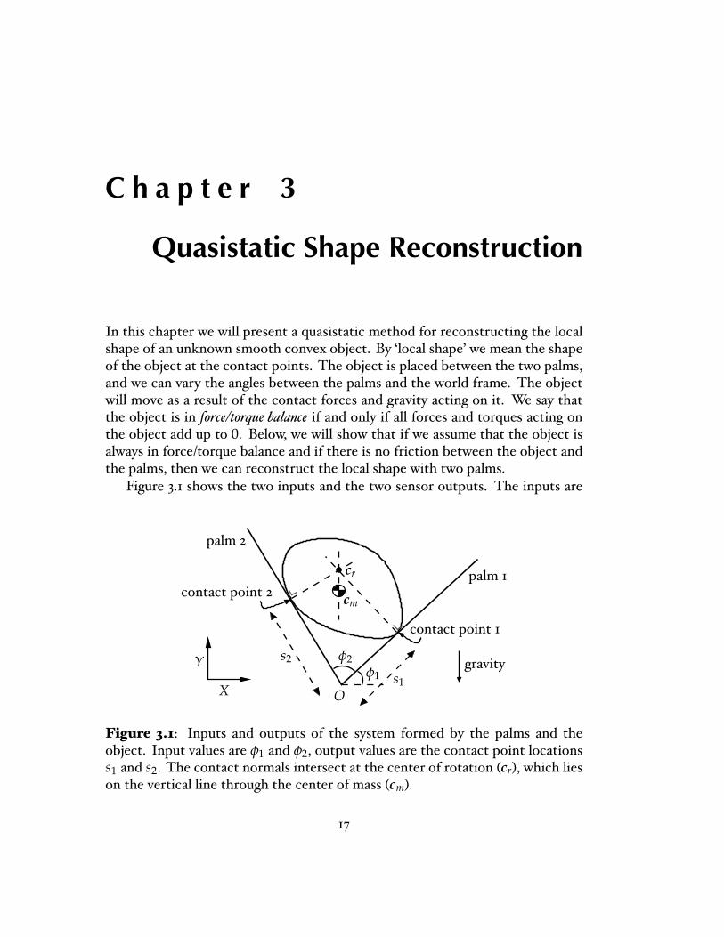
In this chapter we will present a quasistatic method for reconstructing the localshape of an unknown smooth convex object. By `local shape' we mean the shapeof the object at the contact points. The object is placed between the two palms,and we can vary the angles between the palms and the world frame. The objectwill move as a result of the contact forces and gravity acting on it. We say thatthe object is in force/torque balance if and only if all forces and torques acting onthe object add up to 0. Below, we will show that if we assume that the object isalways in force/torque balance and if there is no friction between the object andthe palms, then we can reconstruct the local shape with two palms.Figure 3.1 shows the two inputs and the two sensor outputs. The inputs are

Oφ1

s2

X

Y

palm 2

contact point 1

contact point 2palm 1

gravitys1

φ2

cr

cm

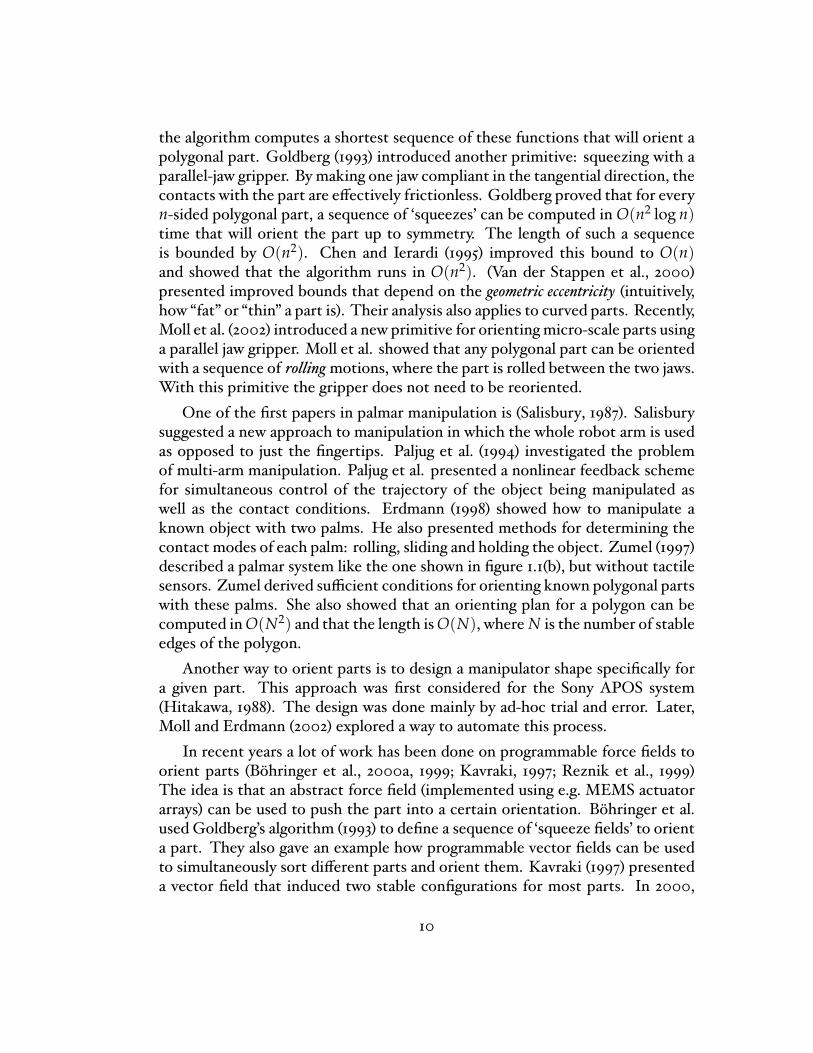
Figure 3.1: Inputs and outputs of the system formed by the palms and theobject. Input values are φ1 and φ2, output values are the contact point locationss1 and s2. The contact normals intersect at the center of rotation (cr), which lieson the vertical line through the center of mass (cm).

17

n(θ)t(θ)

r(θ)x(θ) d(θ)

θφ0object frameOX

global frame

Figure 3.2: The contact support function (r(θ), d(θ)) and the object frame. OXdenotes the X-axis of the object frame.

φ1, the angle between palm 1 and the X-axis of the global frame, and φ2, the anglebetween palm 1 and 2. The tactile sensor elements return the contact points s1and s2 on palm 1 and 2, respectively. Gravity acts in the negative Y direction. Ifthe object is at rest, there is force/torque balance. In that case, since we assumethere is no friction, the lines through the normal forces at the contact pointsand gravity acting on the center of mass intersect at a common point. In otherwords, the sensor values tell us where the X-coordinate of the center of mass isin the global frame. Below we will show that this constraint on the position ofthe center of mass and the constraints induced by the sensor values will allow usto derive an expression for the curvature at the contact points. However, thisexpression depends on the initial position of the center of mass. We can searchfor this position with an initial pose observer that minimizes the error betweenwhat the curvature expression predicts and what the sensor values tell us.

3.1 Notation

Frames We assume that the object is smooth and convex. We also assumethat the origin of the object frame is at the center of mass, and that the center ofmass is in the interior of the object. For every angle θ there exists a unique pointx(θ) on the surface of the object such that the outward pointing normal n(θ)at that point is (cos θ, sin θ)T. This follows from the convexity and smoothnessassumptions. Let the tangent t(θ) be equal to (sin θ,− cos θ)T so that [t, n]constitutes a right-handed frame. Figure 3.2 shows the basic idea. We can also

18

de�ne right-handed frames at the contact points with respect to the palms:

n1 =(− sin φ1, cos φ1

)T

t1 =(

cos φ1, sin φ1)T

and

n2 =(

sin(φ1 + φ2),− cos(φ1 + φ2))T

t2 =(− cos(φ1 + φ2),− sin(φ1 + φ2)

)T

Note that n1 and n2 point into the free space between the palms. Let φ0 be theangle between the object frame and the global frame, such that a rotation matrixR(φ0) maps a point from the object frame to the global frame:

R(φ0) =(

cos φ0 − sin φ0sin φ0 cos φ0

)The object and palm frames are then related in the following way:(

n1 t1)

= −R(φ0)(n(θ) t(θ)

)(n2 t2

)= −R(φ0)

(n(θ + φ2 − π) t(θ + φ2 − π)

)The di�erent frames are shown in �gure 3.3. From these relationships it followsthat

θ = φ1 − φ0 − π2 (3.1)

Di�erentiation We will use `˙' to represent di�erentiation with respect totime t and `′' to represent di�erentiation with respect to a function's parameter.So, for instance, x(θ) = x′(θ)θ. Let v(θ) = ‖x′(θ)‖ be the parameterizationvelocity of the curve x. We can write v(θ) as−x′(θ) · t(θ) and x′(θ) as−v(θ)t(θ).The curvature κ(θ) is de�ned as the turning rate of the curve x(θ). For an

arbitrary curve x the following equality holds (Spivak, 1999a):

t′(θ) = κ(θ)v(θ)n(θ) (3.2)

In our case we have that t′(θ) = n(θ) so it follows that the parameterizationvelocity v(θ) is equal to the radius of curvature 1

κ(θ) at the point x(θ).

19

R0

θ

n1

t(θ+φ2-π)

t1t2

n2

x(θ+φ2-π)

t(θ)n(θ)

n(θ+φ2-π) x(θ)

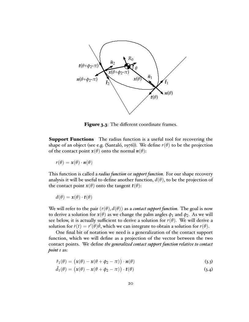
Figure 3.3: The di�erent coordinate frames.

Support Functions The radius function is a useful tool for recovering theshape of an object (see e.g. (Santaló, 1976)). We de�ne r(θ) to be the projectionof the contact point x(θ) onto the normal n(θ):

r(θ) = x(θ) · n(θ)

This function is called a radius function or support function. For our shape recoveryanalysis it will be useful to de�ne another function, d(θ), to be the projection ofthe contact point x(θ) onto the tangent t(θ):

d(θ) = x(θ) · t(θ)

We will refer to the pair (r(θ), d(θ)) as a contact support function. The goal is nowto derive a solution for x(θ) as we change the palm angles φ1 and φ2. As we willsee below, it is actually su�cient to derive a solution for r(θ). We will derive asolution for r(t) = r′(θ)θ, which we can integrate to obtain a solution for r(θ).One �nal bit of notation we need is a generalization of the contact support

function, which we will de�ne as a projection of the vector between the twocontact points. We de�ne the generalized contact support function relative to contactpoint 1 as:

r1(θ) =(x(θ)− x(θ + φ2 − π)

)· n(θ) (3.3)

d1(θ) =(x(θ)− x(θ + φ2 − π)

)· t(θ) (3.4)

20

-d1(θ)

-d2(θ) r1(θ)-r2(θ)

x(θ+φ2-π)

x(θ)

~

~~

~

cm

contact point 1

contact point 2

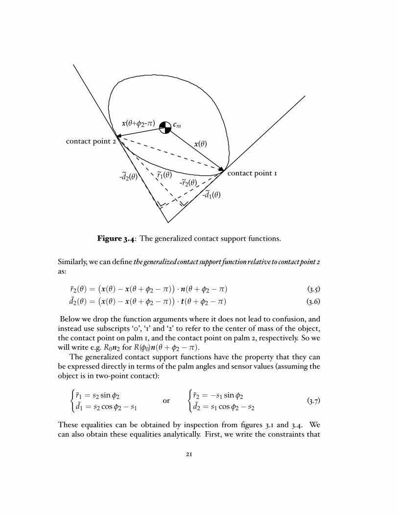
Figure 3.4: The generalized contact support functions.

Similarly, we can de�ne the generalized contact support function relative to contact point 2as:

r2(θ) =(x(θ)− x(θ + φ2 − π)

)· n(θ + φ2 − π) (3.5)

d2(θ) =(x(θ)− x(θ + φ2 − π)

)· t(θ + φ2 − π) (3.6)

Below we drop the function arguments where it does not lead to confusion, andinstead use subscripts `0', `1' and `2' to refer to the center of mass of the object,the contact point on palm 1, and the contact point on palm 2, respectively. So wewill write e.g. R0n2 for R(φ0)n(θ + φ2 − π).The generalized contact support functions have the property that they can

be expressed directly in terms of the palm angles and sensor values (assuming theobject is in two-point contact):{

r1 = s2 sin φ2

d1 = s2 cos φ2 − s1or

{r2 = −s1 sin φ2

d2 = s1 cos φ2 − s2(3.7)

These equalities can be obtained by inspection from �gures 3.1 and 3.4. Wecan also obtain these equalities analytically. First, we write the constraints that

21

two-point contact induces as

s1t1 = cm + R0x1 (3.8)−s2t2 = cm + R0x2, (3.9)

where cm is the position of the center of mass. Next, we can eliminate cm fromthese equations and write

R0 (x1 − x2) = s1t1 + s2t2 (3.10)

The expressions in 3.7 then follow by computing the dot product on both sidesof expression 3.10 with the palm normals and tangents:

r1 = (x1 − x2) · n1 = R0(x1 − x2) · R0n1 = −(s1t1 + s2t2) · n1

= s2 sin φ2 (3.11)d1 = (x1 − x2) · t1 = −(s1t1 + s2t2) · t1 = s2 cos φ2 − s1 (3.12)r2 = (x1 − x2) · n2 = −(s1t1 + s2t2) · n2 = −s1 sin φ2 (3.13)d2 = (x1 − x2) · t2 = −(s1t1 + s2t2) · t2 = s1 cos φ2 − s2 (3.14)

Abovewehave shown that although the generalized contact support functionswere de�ned in the object frame, we can also express them directly in terms ofsensor values and palm angles. This is useful because it can be shown (Erdmann,1999) that the radii of curvature at the contact points can be written in terms ofthe generalized contact support functions as

v1 = −r′2 + d2

sin φ2(3.15)

v2 = −r′1 + d1

sin φ2(3.16)

The derivation of these expressions is included in the appendix. Note thatthese expressions are not su�cient to observe the local shape, even though thegeneralized support functions are directly observable. To observe the shape wewill also need an expression for the time derivative of the function parameters.This is the topic of section 3.3.Equation 3.10 can also be rewritten in terms of the contact support function:

−(r1n1 + d1t1) + (r2n2 + d2t2) = s1t1 + s2t2 (3.17)

22

cm

φ2s2

x1-x2

r1

-d1

s1

r2

d2

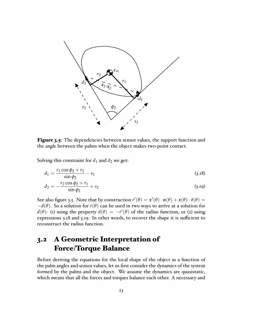
Figure 3.5: The dependencies between sensor values, the support function andthe angle between the palms when the object makes two-point contact.

Solving this constraint for d1 and d2 we get:

d1 =r1 cos φ2 + r2

sin φ2− s1 (3.18)

d2 = −r2 cos φ2 + r1

sin φ2+ s2 (3.19)

See also �gure 3.5. Note that by construction r′(θ) = x′(θ) · n(θ) + x(θ) · t(θ) =−d(θ). So a solution for r(θ) can be used in two ways to arrive at a solution ford(θ): (1) using the property d(θ) = −r′(θ) of the radius function, or (2) usingexpressions 3.18 and 3.19. In other words, to recover the shape it is su�cient toreconstruct the radius function.

3.2 AGeometric Interpretation ofForce/Torque Balance

Before deriving the equations for the local shape of the object as a function ofthe palm angles and sensor values, let us �rst consider the dynamics of the systemformed by the palms and the object. We assume the dynamics are quasistatic,which means that all the forces and torques balance each other. A necessary and

23

su�cient condition for force/torque balance is that the lines through the contactpoints along the contact forces and the line through the center of mass along thegravity vector intersect at one point called the center of rotation (see �gure 3.1). Ifwe move the palms the object will instantaneously rotate around the center ofrotation. The lines through the normals can be described by:

`1 : q1 7→ s1t1 + q1n1 (3.20)`2 : q2 7→ −s2t2 + q2n2 (3.21)

These lines intersect if and only if

q1 =s2 − s1 cos φ2

sin φ2and q2 =

s1 − s2 cos φ2

sin φ2.

Using the generalized contact support functions we can simplify this to q1 =−d2/ sin φ2 and q2 = −d1/ sin φ2. So we can write the following equations forthe center of mass, cm, and the center or rotation, cr:

cm(φ0, φ1, φ2) = s1t1 − R0x1

= −r2t1/ sin φ2 − R0x1 (3.22)cr(φ0, φ1, φ2) = s1t1 + q1n1

= s1t1 − d2n1/ sin φ2

= −(r2t1 + d2n1)/ sin φ2 (3.23)

In appendix A.1 it is shown that the partial derivatives of cm and cr can be writtenas

∂cm

∂φ0= − d2t1

sin φ2−( ∂

∂φ0R0

)x1, (3.24)

∂cr

∂φ0= −

(v1n2 − v2n1 − r2n1 + d2t1

)/ sin φ2. (3.25)

and that we can rewrite equation 3.24 as a function of the relative distancebetween the center of mass and the center of rotation:

∂cm

∂φ0=(

0 −11 0

)(cm − cr) . (3.26)

This last equation should not surprise us. It says that instantaneously the centerof mass rotates around the center of rotation, which is true by de�nition for anypoint on the object.

24

With the results above we can easily describe all the stable poses of an object.We de�ne a stable pose as a local minimum of the potential energy function withrespect to φ0. The potential energy of an object in two-point contact with thepalms is simply the Y coordinate of cm, which can be written as cm ·

(01

). At a

local minimum the �rst derivative with respect to φ0 of this expression will beequal to 0. We can write this condition using equation 3.26 as (cm − cr) ·

(10)

= 0.In other words, at the minima of the potential energy function the X coordinatesof cm and cr have to be equal. Since we assume that the object is always inforce/torque balance and, hence, at a minimum of the potential energy function,we can directly observe the X coordinate of the center of mass. Or, equivalently,we can directly observe the projection onto the X-axis of the vector from thecenter of mass to contact point 1 by using expressions 3.22 and 3.23:

(cm − cr) ·(

10)

= 0

⇒(− r2t1/ sin φ2 − R0x1 + (r2t1 + d2n1)/ sin φ2

)·(

10)

= 0

⇒ (R0x1) ·(

10)

= −d2sin φ1sin φ2

(3.27)

For a local minimum of the potential energy function the Y coordinate of thesecond partial derivative of cm with respect to φ0 has to be greater than 0, i.e.,

∂∂φ0

((cm − cr) ·

(10) )

> 0.

3.3 Recovering Shape

We can write the derivative x(θ) of the function x(θ) that describes the shape asθv(θ)t(θ). So if we can solve for θ, v(θ) and the initial conditions, we can �nd theshape by integrating x. Recall that θ is a curve parameter, so θ is in general notequal to the rotational velocity of the object. We can obtain a simple relationshipbetween θ and φ0 by di�erentiating equation 3.1:

θ = φ1 − φ0 (3.28)

Since we know φ1 solving for θ is equivalent to solving for φ0. In other words, ifwe can observe the curvature at the contact points and the rotational velocity ofthe object, we can recover the shape of an unknown object. By di�erentiating thegeneralized support functionswith respect to time, we can rewrite expressions 3.15

25

and 3.16 for the radii of curvature at the contact points as

v1 = −˙r2 + (θ + φ2)d2

θ sin φ2(3.29)

v2 = −˙r1 + θd1

(θ + φ2) sin φ2(3.30)

See appendix A.1 for details. So to observe the curvature at the contact points,we need to derive an expression for the rotational velocity of the object thatdepends only on palm angles, sensor values and their derivatives. Note that wecan not observe the curvature at the contact point 1 or contact point 2 if θ = 0 orθ + φ2 = 0, respectively. If we can not observe the curvature at a contact point,that point is instantaneously not moving in the object frame.We can recover the rotational velocity by looking at the constraint the force/

torque balance imposes on the motion of the object. Recall equation 3.27:

(R0x1) ·(

10)

= −d2sin φ1sin φ2

(3.31)

The left-hand side of this equation can be rewritten as

(R0x1) ·(

10)

= (R0(r1n1 + d1t1)) ·(

10)

(3.32)= r1 sin φ1 − d1 cos φ1 (3.33)

This expression (implicitly) depends on the orientation of the object. In ap-pendix A.1 it is shown how by di�erentiating this expression and the right-handside of equation 3.31 we can obtain the following expression for the rotationalvelocity of the object:

φ0 =˙r2 cos φ1 − ˙d2 sin φ1 + d2φ2

sin φ12sin φ2

r1 sin φ12 + (r2 + r2) sin φ1 + d2 cos φ1, (3.34)

where φ12 = φ1 + φ2. This expression for φ0 depends on the control inputs,the sensor values, their derivatives and the current values of radius function atthe contact points. The system of di�erential equations describing the (sensed)shape and motion can be summarized as follows:

r1 = −d1(φ1 − φ0) (3.35)r2 = −d2(φ12 − φ0) (3.36)

φ0 =˙r2 cos φ1 − ˙d2 sin φ1 + d2φ2

sin φ12sin φ2

r1 sin φ12 + (r2 + r2) sin φ1 + d2 cos φ1(3.37)

26

The �rst two equations describe the rate of change of the radius function atthe contact points. The radius function uniquely de�nes the shape of the object.Equation 3.37 describes the motion of the object. If the object remains in contactwith both palms, it has only one degree of freedom. So knowing just the rotationalvelocity is su�cient.So far we have assumed that we have sensor data that is continuous and

without any error. In practice sensors will be discrete, both in time and space,and there will also be errors. We would like to recover the shape of an unknownobject in such a setting as well. There are two main directly observable errorterms at each time step. First, one can check the error in the force/torque balanceconstraint (equation 3.31). Let that error be denoted by e f . So at a given time t,e f (t) is equal to

e f (t) =((R0(φ0)x1) ·

(10)

+ d2sin φ1sin φ2

), (3.38)

where ` ' denotes the estimated value of a variable. The second observable erroris the error in the two-point contact constraint (equation 3.10). Let this error bedenoted by ec. In other words,

ec(t) =(

R0(φ0)(x1 − x2)− s1t1 − s2t2)

(3.39)

Our program searches for the initial conditions of our system by minimizing thesum of all directly observable errors.In our current implementationwe use a fourth-orderAdams-Bashforth-Moul-

ton predictor-corrector method to integrate equations 3.35�3.37. Let the state bede�ned as the vector (r1, r2, φ0)T. In the prediction step the state at time t − 1and derivatives at time t− 3, t− 2, and t− 1 are used to predict the state at timet. In the correction step, we use the state estimate at t − 1 and derivatives att− 3, . . . , t to re�ne the state estimate at time t. The correction step is repeateduntil the relative change in the estimate is below a certain threshold or if amaximum number of iterations has been reached. This high-order method tendsto �lter out most of the noise and numerical errors. In our simulation resultshardly any error accumulates during integration (see section 3.4).

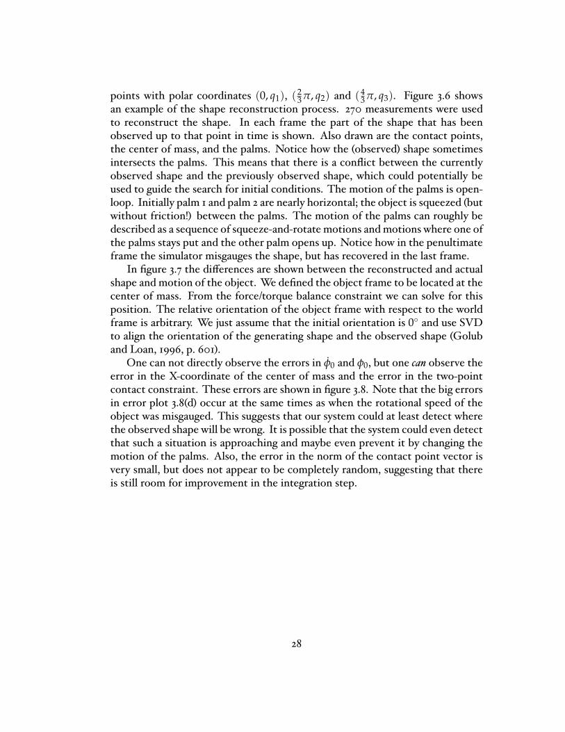
3.4 SimulationResultsThe results in this section are based on numerical simulation in Matlab. Wegenerate random test shapes in the following way. We pick three numbers q1,q2, and q3 independently and uniformly random from the interval [0.1, 2.5]. Arandom shape is generated by computing a closed spline interpolation of the

27

points with polar coordinates (0, q1), (23 π, q2) and (4

3 π, q3). Figure 3.6 showsan example of the shape reconstruction process. 270 measurements were usedto reconstruct the shape. In each frame the part of the shape that has beenobserved up to that point in time is shown. Also drawn are the contact points,the center of mass, and the palms. Notice how the (observed) shape sometimesintersects the palms. This means that there is a con�ict between the currentlyobserved shape and the previously observed shape, which could potentially beused to guide the search for initial conditions. The motion of the palms is open-loop. Initially palm 1 and palm 2 are nearly horizontal; the object is squeezed (butwithout friction!) between the palms. The motion of the palms can roughly bedescribed as a sequence of squeeze-and-rotate motions andmotions where one ofthe palms stays put and the other palm opens up. Notice how in the penultimateframe the simulator misgauges the shape, but has recovered in the last frame.In �gure 3.7 the di�erences are shown between the reconstructed and actual

shape and motion of the object. We de�ned the object frame to be located at thecenter of mass. From the force/torque balance constraint we can solve for thisposition. The relative orientation of the object frame with respect to the worldframe is arbitrary. We just assume that the initial orientation is 0◦ and use SVDto align the orientation of the generating shape and the observed shape (Goluband Loan, 1996, p. 601).One can not directly observe the errors in φ0 and φ0, but one can observe the

error in the X-coordinate of the center of mass and the error in the two-pointcontact constraint. These errors are shown in �gure 3.8. Note that the big errorsin error plot 3.8(d) occur at the same times as when the rotational speed of theobject was misgauged. This suggests that our system could at least detect wherethe observed shape will be wrong. It is possible that the system could even detectthat such a situation is approaching and maybe even prevent it by changing themotion of the palms. Also, the error in the norm of the contact point vector isvery small, but does not appear to be completely random, suggesting that thereis still room for improvement in the integration step.

28

t=0.03 t=0.07 t=0.11 t=0.14

t=0.18 t=0.22 t=0.26 t=0.29

t=0.33 t=0.37 t=0.41 t=0.44

t=0.48 t=0.52 t=0.55 t=0.59

t=0.63 t=0.67 t=0.70 t=0.74

t=0.78 t=0.81 t=0.85 t=0.89

t=0.93 t=0.96 t=1.00

Figure 3.6: The frames show the reconstructed shape after 10, 20,. . . ,270 mea-surements. The three large dots indicate the center of mass and the contactpoints at each time, the smaller dots show the part of the shape that has beenreconstructed at that time.

29

(a) The actual shape and the observedshape.

0 0.2 0.4 0.6 0.8 120

30

40

50

60

70

t

r1

r2

observed r1

observed r2

(b) The actual and observed values of theradius function (in mm).

0 0.2 0.4 0.6 0.8 1�1.5

�1

�0.5

0

0.5

1

1.5

2

t

φ0 observed φ0

(c) The actual and observed orientation ofthe object.

0 0.2 0.4 0.6 0.8 1

�40

�20

0

20

40

60

t

dφ0 /dt observed d /dtφ0

(d) The actual and observed rotational ve-locity of the object.

Figure 3.7: The di�erences between the actual and observed shape.

30

0 0.2 0.4 0.6 0.8 1−500

0

500

1000

t

(a) The real and observed X-coordinateof the center of mass (in mm)

0 0.2 0.4 0.6 0.8 110

20

30

40

50

60

70

80

90

t

(b) The real and observed norm of thevector between the contact points (inmm)

0 0.2 0.4 0.6 0.8 1−3

−2

−1

0

1

2

3

t

(c) The error in the X-coordinate of thecenter of mass (in mm)

0 0.2 0.4 0.6 0.8 1−0.03

−0.02

−0.01

0

0.01

0.02

0.03

t

(d) The error in the norm of the vectorbetween the contact points (in mm)

Figure 3.8: The observable error for the reconstructed shape.

31

−300 −200 −100 0 100 200 300−200

−150

−100

−50

0

50

100

150

200

X

Y

(a) The contact point of a marble being rolled on a touchpad.X and Y are measured in `tactels.'

0 500 1000 1500 2000 25000

0.005

0.01

0.015

0.02

0.025

measurement number

time

betw

een

cons

ecut

ive

mea

sure

men

ts

(b) The speed at which measurements are reported. The aver-age time betweenmeasurements is 0.010 seconds, the standarddeviation is 0.0050.

Figure 3.9: Resolution and sensing frequency of the VersaPad.

32

Figure 3.10: Setup of the palms.

3.5 Experimental ResultsThe tactile sensors we are using are touchpads made by Interlink Electronics(http://www.interlinkelec.com). These touchpads are most commonly used innotebook computers. They use so-called force sensing resistors to measure thelocation and the applied pressure at the contact point. One of the advantages ofthis technology, according to Interlink, is that it does not su�er as much fromelectrostatic contamination as capacitance-based touchpads. If there is morethan one contact point, the pad returns the centroid. The physical pad hasa resolution of 1000 counts per inch (cpi) in the X and Y direction, but the�rmware limits the resolution to 200 cpi. It can report 128 pressure levels, butthe pressure readings are not very reliable. In our experiments we only usedthe coordinates of the contact point and ignored the pressure data. The padmeasures 55.5 × 39.5mm2. Sensor data can be read out through a rs232 serialport connection.Figure 3.9 shows the results of a simple test to establish the feasibility of

the touchpad. The test consisted of rolling a marble around on the touchpadand tracking the contact point. Figure 3.9(a) shows the `curve' traced out by thecontact point. Figure 3.9(b) shows how fast we can get sensor readings from thetouchpad. Notice how the times between measurements are roughly centeredaround 3 bands. This could be related to the way our driver polls the touchpadfor data; further tweaking might increase the speed at which measurements arereported.

33

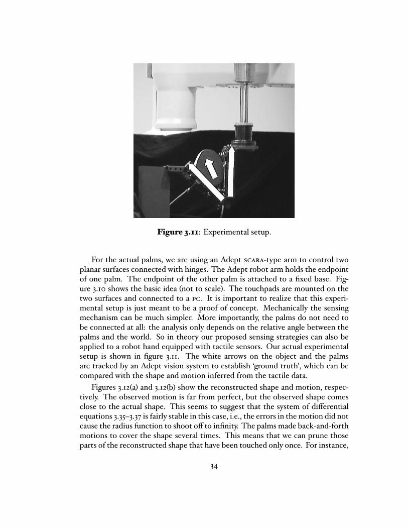
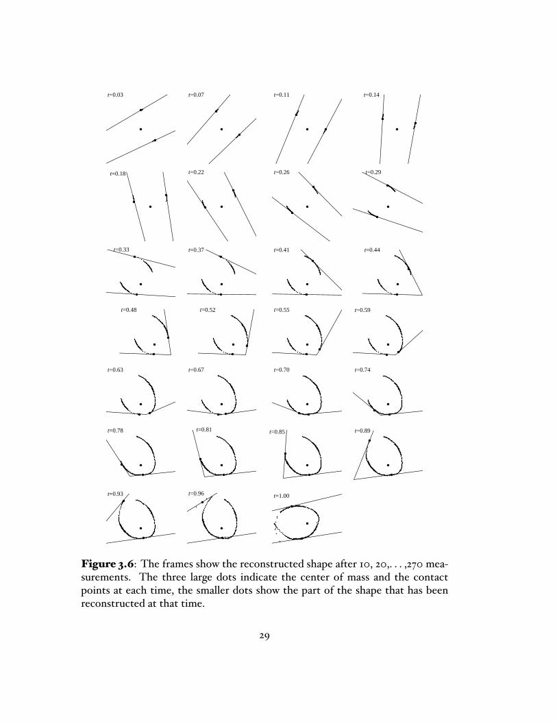
Figure 3.11: Experimental setup.

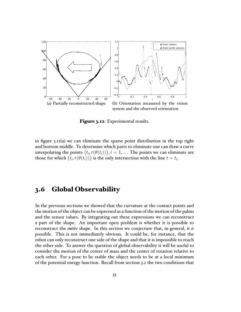
For the actual palms, we are using an Adept scara-type arm to control twoplanar surfaces connected with hinges. The Adept robot arm holds the endpointof one palm. The endpoint of the other palm is attached to a �xed base. Fig-ure 3.10 shows the basic idea (not to scale). The touchpads are mounted on thetwo surfaces and connected to a pc. It is important to realize that this experi-mental setup is just meant to be a proof of concept. Mechanically the sensingmechanism can be much simpler. More importantly, the palms do not need tobe connected at all: the analysis only depends on the relative angle between thepalms and the world. So in theory our proposed sensing strategies can also beapplied to a robot hand equipped with tactile sensors. Our actual experimentalsetup is shown in �gure 3.11. The white arrows on the object and the palmsare tracked by an Adept vision system to establish `ground truth', which can becompared with the shape and motion inferred from the tactile data.Figures 3.12(a) and 3.12(b) show the reconstructed shape and motion, respec-

tively. The observed motion is far from perfect, but the observed shape comesclose to the actual shape. This seems to suggest that the system of di�erentialequations 3.35�3.37 is fairly stable in this case, i.e., the errors in themotion did notcause the radius function to shoot o� to in�nity. The palms made back-and-forthmotions to cover the shape several times. This means that we can prune thoseparts of the reconstructed shape that have been touched only once. For instance,

34

−60 −40 −20 0 20 40 600

20

40

60

80

100

120

(a) Partially reconstructed shape0 0.2 0.4 0.6 0.8 1

−0.4

−0.2

0

0.2

0.4

0.6

0.8

1

1.2

t

ψ from camera ψ from tactile sensors

(b) Orientation measured by the visionsystem and the observed orientation

Figure 3.12: Experimental results.

in �gure 3.12(a) we can eliminate the sparse point distribution in the top rightand bottom middle. To determine which parts to eliminate one can draw a curveinterpolating the points

(ti, r(θ(ti))

), i = 1, . . . The points we can eliminate are

those for which(ti, r(θ(ti))

)is the only intersection with the line t = ti.

3.6 Global Observability

In the previous sections we showed that the curvature at the contact points andthemotion of the object can be expressed as a function of themotion of the palmsand the sensor values. By integrating out these expressions we can reconstructa part of the shape. An important open problem is whether it is possible toreconstruct the entire shape. In this section we conjecture that, in general, it ispossible. This is not immediately obvious. It could be, for instance, that therobot can only reconstruct one side of the shape and that it is impossible to reachthe other side. To answer the question of global observability it will be useful toconsider the motion of the center of mass and the center of rotation relative toeach other. For a pose to be stable the object needs to be at a local minimumof the potential energy function. Recall from section 3.2 the two conditions that

35

φ1 = 0

φ1 + φ2 = πoutside boundary

inside boundary

φ2 = 0

φ1

φ2

φ0

(a) The stable pose surface in con�guration space

(b) The generating object shape

Figure 3.13: Stable poses for a particular shape. Note that only one 2π periodof φ0 is shown in (a) and the surface extends from −∞ to ∞ in the φ0 direction,i.e., the inside and outside boundary do not meet.

have to hold for a stable pose:

(cm − cr) ·(

10

)= 0, (3.40)

∂

∂φ0

((cm − cr) ·

(10

) )= 0. (3.41)

36

The stable poses induce a two-dimensional subset of the (φ1, φ2, φ0)-con�gura-tion space. Figure 3.13 shows all the stable poses for a given shape. These stablecon�gurations form a spiraling surface. From �gure 3.13 it follows that for thisparticular shape it is indeed possible to reconstruct the entire shape, becausethere exists a path on the surface of stable con�gurations between any two stablecon�gurations. We suspect that this is true in general. Although we do not havea complete proof for it, we will give some intuition for the following conjecture:

For any smooth convex shape there exists a surface of stable con�gu-rations such that we can bring the object from any orientation to anyother orientation by moving along a curve embedded in this surface.

We argue in favor of this conjecture by considering the boundaries of the stablecon�guration surface. Let us de�ne the inside boundary as those con�gurationswhere both the �rst and second derivative with respect to φ0 of the potentialenergy function vanish. Using expressions 3.22�3.27 we can write these twoconstraints as:

(cm − cr) ·(

10

)= −d2 sin φ1/ sin φ2 −

( cos φ0− sin φ0

)· x1 = 0, (3.42)

∂

∂φ0

((cm − cr) ·

(10

))=

v1 sin(φ1 + φ2) + (v2 + r2) sin φ1

sin φ2+(sin φ0

cos φ0

)· x1 = 0.

(3.43)

The outside boundary of the stable con�guration surface is determined by limits onthe palm angles: φ1, φ2 > 0 and φ1 + φ2 < π. These limits can be geometricallyinterpreted as follows:

φ1 = 0+, 0 < φ2 < π: When φ2 = π−, both palms are nearly horizontal,pointing in nearly opposite directions. In the limit, as φ2 approachesπ, s1 = s2 = 0, and the contact point is an extremum of the radiusfunction (since the center of mass is right above the contact point andtherefore r′(θ) = −d(θ) = 0). As φ2 decreases, contact point 2 coversnearly half the shape. As φ2 approaches 0, the palms form an antipodalgrasp. The contact points are then at a minimum of the diameter functionD(θ)

def≡ r(θ) + r(θ − π).

φ2 = 0+, 0 < φ1 < π: When φ1 = 0+, this boundary usually connects to theprevious one. As φ1 increases, the palmsmaintain an antipodal grasp, so thecontact points do not change. As φ1 approaches π, palm 1 and 2 both pointto the left. Below we will describe when this boundary and the previousone do not connect. This case is where our argument breaks down.

37

21

34

Figure 3.14: Plan for observing the entire shape of an unknown object.

0 < φ1 < π, φ2 = π− − φ1: This case is symmetrical to the �rst one. Nowcontact point 1 covers nearly half the shape.

From this geometric interpretation it is clear that we can bring the object toany orientation by moving along these outside boundaries. More importantly,by following these boundaries we can reconstruct the entire shape. Figure 3.14shows how a shape is reconstructed by palms that trace these boundaries. Firstpalm 2 sweeps through its entire range ofmotionwhile palm 1 is nearly horizontal.Then palm 1 sweeps through its range. Finally both palms move simultaneouslyback to their original position. The object is now rotated roughly 180◦. Thepart of the shape that has been reconstructed is drawn in black. We can repeatthis plan to re�ne the estimate of the shape. However, these boundaries arethemselves not part of the surface, so the question is whether there always existstable con�gurations arbitrarily close to the outside boundary. The answer is�yes�, provided the inside and outside boundary do not meet. Let a generic smooth convexobject be de�ned as a smooth convex object in general position such that none ofthe singular cases described below apply. Below we will argue that for a genericsmooth convex shape the inside boundary never (with probability 1) meets theoutside boundary and, hence, there exists a path on the surface connecting anytwo orientations of the object. For each outside boundary condition we can

38

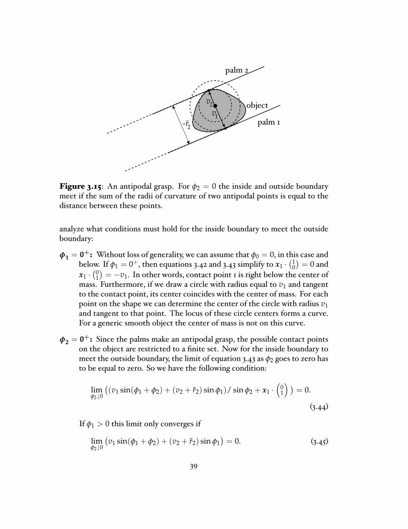
-r

v

~v1

2

2palm 1

palm 2

object

Figure 3.15: An antipodal grasp. For φ2 = 0 the inside and outside boundarymeet if the sum of the radii of curvature of two antipodal points is equal to thedistance between these points.

analyze what conditions must hold for the inside boundary to meet the outsideboundary:

φ1 = 0+: Without loss of generality, we can assume that φ0 = 0, in this case andbelow. If φ1 = 0+, then equations 3.42 and 3.43 simplify to x1 ·

(10)

= 0 andx1 ·

(01)

= −v1. In other words, contact point 1 is right below the center ofmass. Furthermore, if we draw a circle with radius equal to v1 and tangentto the contact point, its center coincides with the center of mass. For eachpoint on the shape we can determine the center of the circle with radius v1and tangent to that point. The locus of these circle centers forms a curve.For a generic smooth object the center of mass is not on this curve.

φ2 = 0+: Since the palms make an antipodal grasp, the possible contact pointson the object are restricted to a �nite set. Now for the inside boundary tomeet the outside boundary, the limit of equation 3.43 as φ2 goes to zero hasto be equal to zero. So we have the following condition:

limφ2↓0

((v1 sin(φ1 + φ2) + (v2 + r2) sin φ1)/ sin φ2 + x1 ·

(01

) )= 0.

(3.44)

If φ1 > 0 this limit only converges if

limφ2↓0

(v1 sin(φ1 + φ2) + (v2 + r2) sin φ1

)= 0. (3.45)

39

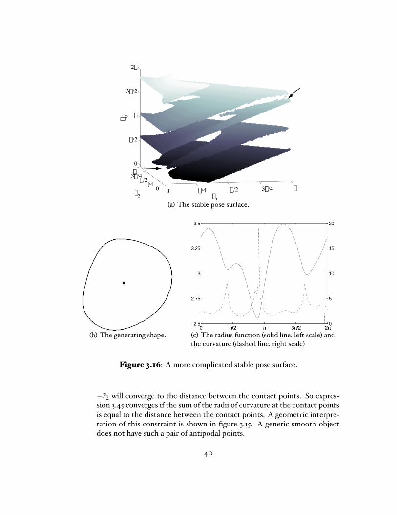
0 p/4 p/2 3p/4 p0p/4

p/23p/4p0

p/2

p

3p/2

2p

f1f2

f 0

(a) The stable pose surface.

(b) The generating shape.0 π/2 π 3π/2 2π

2.5

2.75

3

3.25

3.5

0 π/2 π 3π/2 2π0

5

10

15

20

(c) The radius function (solid line, left scale) andthe curvature (dashed line, right scale)

Figure 3.16: A more complicated stable pose surface.

−r2 will converge to the distance between the contact points. So expres-sion 3.45 converges if the sum of the radii of curvature at the contact pointsis equal to the distance between the contact points. A geometric interpre-tation of this constraint is shown in �gure 3.15. A generic smooth objectdoes not have such a pair of antipodal points.

40

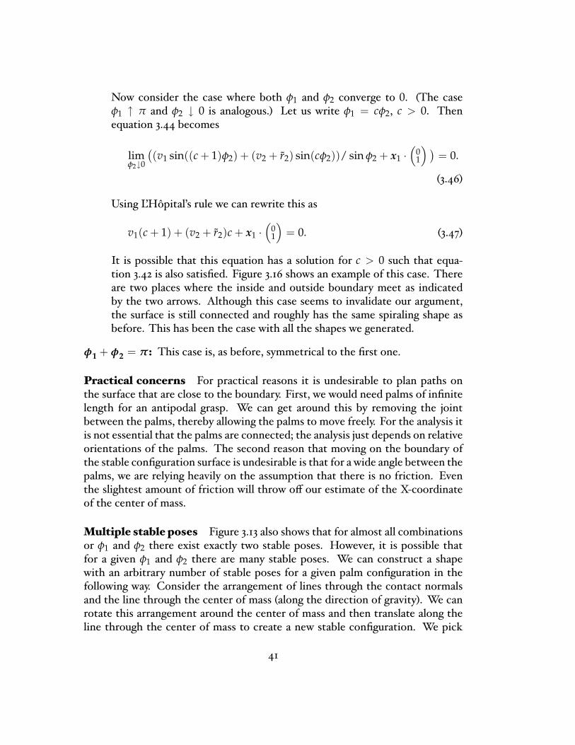
Now consider the case where both φ1 and φ2 converge to 0. (The caseφ1 ↑ π and φ2 ↓ 0 is analogous.) Let us write φ1 = cφ2, c > 0. Thenequation 3.44 becomes

limφ2↓0

((v1 sin((c + 1)φ2) + (v2 + r2) sin(cφ2))/ sin φ2 + x1 ·

(01

) )= 0.

(3.46)

Using L'Hôpital's rule we can rewrite this as

v1(c + 1) + (v2 + r2)c + x1 ·(

01

)= 0. (3.47)

It is possible that this equation has a solution for c > 0 such that equa-tion 3.42 is also satis�ed. Figure 3.16 shows an example of this case. Thereare two places where the inside and outside boundary meet as indicatedby the two arrows. Although this case seems to invalidate our argument,the surface is still connected and roughly has the same spiraling shape asbefore. This has been the case with all the shapes we generated.

φ1 + φ2 = π: This case is, as before, symmetrical to the �rst one.

Practical concerns For practical reasons it is undesirable to plan paths onthe surface that are close to the boundary. First, we would need palms of in�nitelength for an antipodal grasp. We can get around this by removing the jointbetween the palms, thereby allowing the palms to move freely. For the analysis itis not essential that the palms are connected; the analysis just depends on relativeorientations of the palms. The second reason that moving on the boundary ofthe stable con�guration surface is undesirable is that for a wide angle between thepalms, we are relying heavily on the assumption that there is no friction. Eventhe slightest amount of friction will throw o� our estimate of the X-coordinateof the center of mass.

Multiple stable poses Figure 3.13 also shows that for almost all combinationsor φ1 and φ2 there exist exactly two stable poses. However, it is possible thatfor a given φ1 and φ2 there are many stable poses. We can construct a shapewith an arbitrary number of stable poses for a given palm con�guration in thefollowing way. Consider the arrangement of lines through the contact normalsand the line through the center of mass (along the direction of gravity). We canrotate this arrangement around the center of mass and then translate along theline through the center of mass to create a new stable con�guration. We pick

41

palm 2 palm 1

Figure 3.17: Many stable poses are possible for a given palm con�guration thatproduce the same sensor readings.

the new contact points to be at the same distance from the intersection of thelines as in the original arrangement. This means that this new con�gurationproduces the same sensor readings as well. We can repeat this process, pickinga di�erent amount of translation at each step to create an arbitrary number ofstable con�gurations. We can create a smooth convex shape that has these stableposes in the following way. Consider the convex polygon that has the contactpoints of all these stable poses as vertices. If such a polygon does not exist weremove the poses that cause the concavities. The arrangement of lines describedabove corresponds to critical points of the potential energy function. To makesure that all the critical points are local minima we need to consider the secondderivative of the potential energy function (see equation 3.43). For each contactpoint we can pick the radius of curvature to be arbitrarily large such that thesecond derivative is greater than 0. We can locally deform the polygon aroundeach vertex such that at the contact point the radius of curvature is as desiredand the shape remains convex. Figure 3.17 illustrates this geometric construction.Since the polygon induced by the contact points is convex, there exists a smoothconvex shape with these stable poses.

42

3.7 Segmentation of ShapeReconstructionIt is possible that the object undergoes a discrete change in orientation as thepalms move. This happens when the system reaches a boundary of the stablepose surface in the (φ1, φ2, φ0)-con�guration space. In terms of �gure 3.13, theobject �falls o�� the stable pose surface. When this happens we need to restartour shape reconstruction process. Sudden changes in orientation give rise to twoproblems:

� How do we decide that the object is undergoing a discrete change in ori-entation? Since the sensor values are reported at a certain frequency, everymeasurement corresponds to a discrete change in orientation. More im-portantly, the sensor readings are likely to be noisy, so one spike in themeasurements doesn't necessarily mean that a jump in the orientation oc-curred.

� Given a set of reconstructed shape segments, how do we piece them to-gether? We have to �nd a method for determining the relative positionsof the di�erent segments. Also, if some segments overlap, we need toconsolidate the possibly con�icting values for the radius function.

For the �rst problem we can use the following approach. If the object un-dergoes a discrete change in orientation, numerical integration of φ0 will be veryunstable. The predictor-corrector method will generally not be able to recoverand φ0 shoots o� to in�nity. So we can trigger a restart of the observer if φ0exceeds a certain threshold. This means that the observer is also restarted ifthere is a large error in the sensor data. Often there will be a sequence of spikesif the object's motion approaches a singularity. To prevent the creation of manytiny segments, we therefore also set a limit on theminimum segment length. Thesearch for the initial conditions at the start of each segment is seeded with theendpoint of the previous segment.For the initial segment we only have to search for the vertical o�set of the

center of mass with respect to the center of rotation at the start of the segment,since we are free to choose a particular orientation. But for subsequent segmentsthe relative orientation with respect to this initial segment matters. So now wehave to search for two unknowns for each segment: the relative orientation andthe o�set at the start of each segment.Implicit in these segments there is still a temporal dependence: each segment

consists of a temporal sequence of measurements. It will be useful for the shapereconstruction to eliminate this temporal dependence. We therefore introducethe notion of a patch. A patch is de�ned as an approximation of the radius

43

error

segment 2

segment 1

Figure 3.18: The error of two (radially) overlapping segments is equal to thearea between them.

function on a domain [θ1, θ2]. We map a segment to a set of patches in thefollowing way. Suppose we have a segment S consisting of nmeasurements. Eachmeasurement is of the form (ti, θi, ri), i = 1, . . . , n. We divide the segment Sinto smaller segments S1, . . . , Sm at the m extrema of the (ti, θi) sequence. Ifthere are extrema, then the same part of the shape is covered more than once.Due to numerical errors and noise each time a part of the shape is covered theapproximation will look slightly di�erent. We therefore create a patch for eachtime a particular part of the shape is observed and consolidate patches withoverlapping domains at a later stage. For each Sj, j = 1, . . . , m, we create a patchPj. The domain of Pj is de�ned as the closed interval ranging from the minimumto the maximum θ value in Sj's measurements. The approximation of the radiusfunction is simply de�ned as the spline interpolation through Pj's observed valuesof the radius function.

In addition to the locally observable errors, we can also de�ne a global errorterm as a function of a particular arrangement of segments: we can compute thearea between con�icting sections of the segments and take that to be the errorof the arrangement (see �gure 3.18). For a given arrangement of segments wecan compute all the patches as described above. If none of the patches overlap(radially), the error is equal to 0. Now suppose some of them do overlap. Let[θ1, θ2] be a domain for which k patches P1, . . . , Pk overlap. Let P be the averageof the k patches. Then we can de�ne the area error on [θ1, θ2] to be equal to the

44

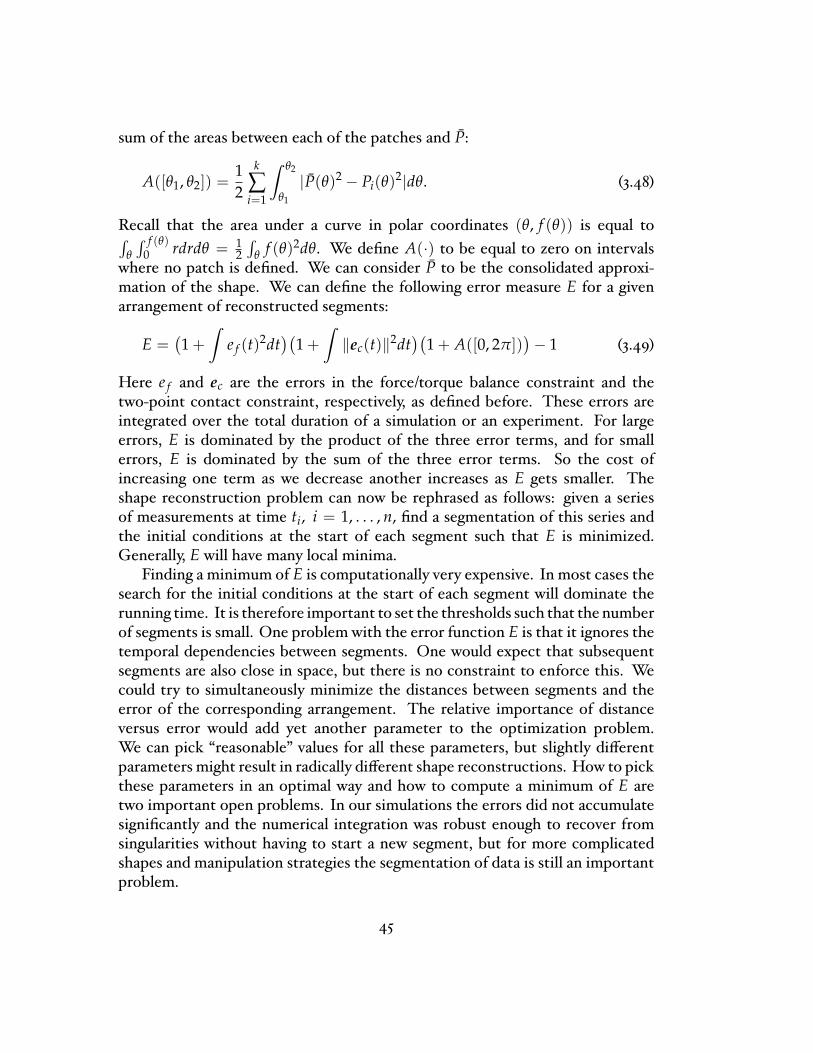
sum of the areas between each of the patches and P:

A([θ1, θ2]) =12

k

∑i=1

∫ θ2

θ1

|P(θ)2 − Pi(θ)2|dθ. (3.48)

Recall that the area under a curve in polar coordinates (θ, f (θ)) is equal to∫θ

∫ f (θ)0 rdrdθ = 1

2

∫θ f (θ)2dθ. We de�ne A(·) to be equal to zero on intervals

where no patch is de�ned. We can consider P to be the consolidated approxi-mation of the shape. We can de�ne the following error measure E for a givenarrangement of reconstructed segments:

E =(1 +

∫e f (t)2dt

)(1 +

∫‖ec(t)‖2dt

)(1 + A([0, 2π])

)− 1 (3.49)

Here e f and ec are the errors in the force/torque balance constraint and thetwo-point contact constraint, respectively, as de�ned before. These errors areintegrated over the total duration of a simulation or an experiment. For largeerrors, E is dominated by the product of the three error terms, and for smallerrors, E is dominated by the sum of the three error terms. So the cost ofincreasing one term as we decrease another increases as E gets smaller. Theshape reconstruction problem can now be rephrased as follows: given a seriesof measurements at time ti, i = 1, . . . , n, �nd a segmentation of this series andthe initial conditions at the start of each segment such that E is minimized.Generally, E will have many local minima.Finding a minimum of E is computationally very expensive. In most cases the

search for the initial conditions at the start of each segment will dominate therunning time. It is therefore important to set the thresholds such that the numberof segments is small. One problem with the error function E is that it ignores thetemporal dependencies between segments. One would expect that subsequentsegments are also close in space, but there is no constraint to enforce this. Wecould try to simultaneously minimize the distances between segments and theerror of the corresponding arrangement. The relative importance of distanceversus error would add yet another parameter to the optimization problem.We can pick �reasonable� values for all these parameters, but slightly di�erentparameters might result in radically di�erent shape reconstructions. How to pickthese parameters in an optimal way and how to compute a minimum of E aretwo important open problems. In our simulations the errors did not accumulatesigni�cantly and the numerical integration was robust enough to recover fromsingularities without having to start a new segment, but for more complicatedshapes and manipulation strategies the segmentation of data is still an importantproblem.

45

C h a p t e r 4

Dynamic Shape Reconstruction

In this chapter we drop the assumption that force/torque balance is maintained atall time. It turns out that it is still possible to observe the shape, but now we willneed to consider second-order e�ects. We will need to model the accelerations,forces, and torques that occur in our system. Our approach is to construct anobserver for our system. The notion of an observer will be explained later onin more detail, but for now one can think of an observer as an (on-line) stateestimator that given an estimate quickly converges to the true state as timeprogresses. The construction of an observer requires several steps. The �rst stepis to write our system in the following form:

q = f (q) + τ1g1(q) + τ2g2(q), (4.1)y = h(q) (4.2)

where q is a state vector, f , g1 and g2 are vector �elds, and h is called the outputfunction. In our case, the state is a vector of sensor readings and the con�gurationof the system. The con�guration is de�ned by the orientations of the palms. Theoutput function returns (a function of ) the sensor readings. The vector �eldsg1 and g2 are called the input vector �elds and describe the rate of change of oursystem as torques are being applied on palm 1 and palm 2, respectively, at theirpoint of intersection. The vector �eld f is called the drift vector �eld. It includesthe e�ects of gravity.The second step is to �nd out whether the system described by equations 4.1

and 4.2 is observable. Informally, this notion can be de�ned as: a system isobservable if for any twodi�erent states the output functionwill return a di�erentvalue after some time.The �nal step is then to construct the actual observer, which is basically a

control law. We can estimate the initial state and if our estimate is not too farfrom the true initial state, the observer will rapidly converge to the actual state.

47

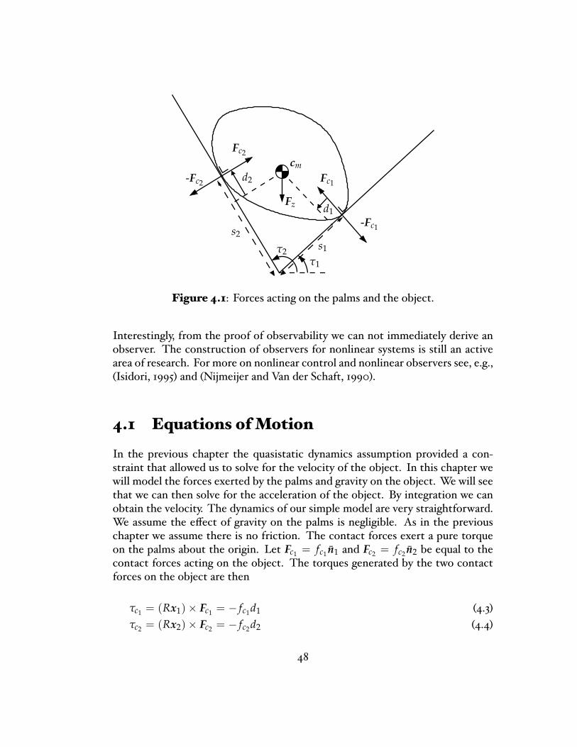
s1τ1

-Fc1

τ2

Fz

-Fc2

Fc2

Fc1

d1

d2

s2

cm

Figure 4.1: Forces acting on the palms and the object.

Interestingly, from the proof of observability we can not immediately derive anobserver. The construction of observers for nonlinear systems is still an activearea of research. For more on nonlinear control and nonlinear observers see, e.g.,(Isidori, 1995) and (Nijmeijer and Van der Schaft, 1990).

4.1 Equations ofMotion

In the previous chapter the quasistatic dynamics assumption provided a con-straint that allowed us to solve for the velocity of the object. In this chapter wewill model the forces exerted by the palms and gravity on the object. We will seethat we can then solve for the acceleration of the object. By integration we canobtain the velocity. The dynamics of our simple model are very straightforward.We assume the e�ect of gravity on the palms is negligible. As in the previouschapter we assume there is no friction. The contact forces exert a pure torqueon the palms about the origin. Let Fc1 = fc1 n1 and Fc2 = fc2 n2 be equal to thecontact forces acting on the object. The torques generated by the two contactforces on the object are then

τc1 = (Rx1)× Fc1 = − fc1d1 (4.3)τc2 = (Rx2)× Fc2 = − fc2d2 (4.4)

48

The dynamics of the system are described by the following equations (see also�gure 4.1):

ma0 = Fz + Fc1 + Fc2 (4.5)I0α0 = τc1 + τc2 = − fc1d1 − fc2d2, fc1 , fc2 ≥ 0 (4.6)I1α1 = τ1 − fc1s1 (4.7)

I2(α1 + α2) = τ2 + fc2s2 (4.8)

Here the subscript i, (i = 0, 1, 2) refers to the object, palm 1 and palm 2, re-spectively. Fz = mg is the gravitational force on the object. Note that α2 is theangular acceleration of palm 2 measured with respect to palm 1, so that φ2 = α2.Solving for a0 and α0, we get

a0 = − I1α1 − τ1

ms1n1 +

I2(α1 + α2)− τ2

ms2n2 + g (4.9)

α0 =I1α1 − τ1

mρ2s1d1 −

I2(α1 + α2)− τ2

mρ2s2d2 (4.10)

where ρ =√

I0/m is the radius of gyration of the object.We can measure the mass m by letting the object come to rest. In that case

a0 = 0 and we can solve for m by using m = −(Fc1 + Fc2)/g. We have to solvefor the radius of gyration by other means, shown in the next section. The massproperties of the palms are assumed to be known.

4.2 General CaseWe will now rewrite the constraints on the shape and motion of the object inthe form of equation 4.1. We will introduce the state variables ω0, ω1 and ω2to denote φ0, φ1 and φ2, respectively. The other state variables are: s1, s2, r1,r2, and ρ. So the shape at the contact points is represented by the values of theradius function at the contact points. Note that r1 and r2 are reparametrizationsof the radius function as a function of time instead of θ. So even though shapeis thought of as being time invariant, our representation describes shape as therate of change in the radius function values at the contact points. The inputs toour system are the torques produced by the motors of the palms. The outputsare the sensor values. As we will see below, obtaining expressions for s1 and s2 isquite involved, while obtaining expressions for the derivatives of the other statevariables is straightforward. Recall the position constraint on contact point 1(equation 3.8):

s1t1 = cm + Rx1 (4.11)

49

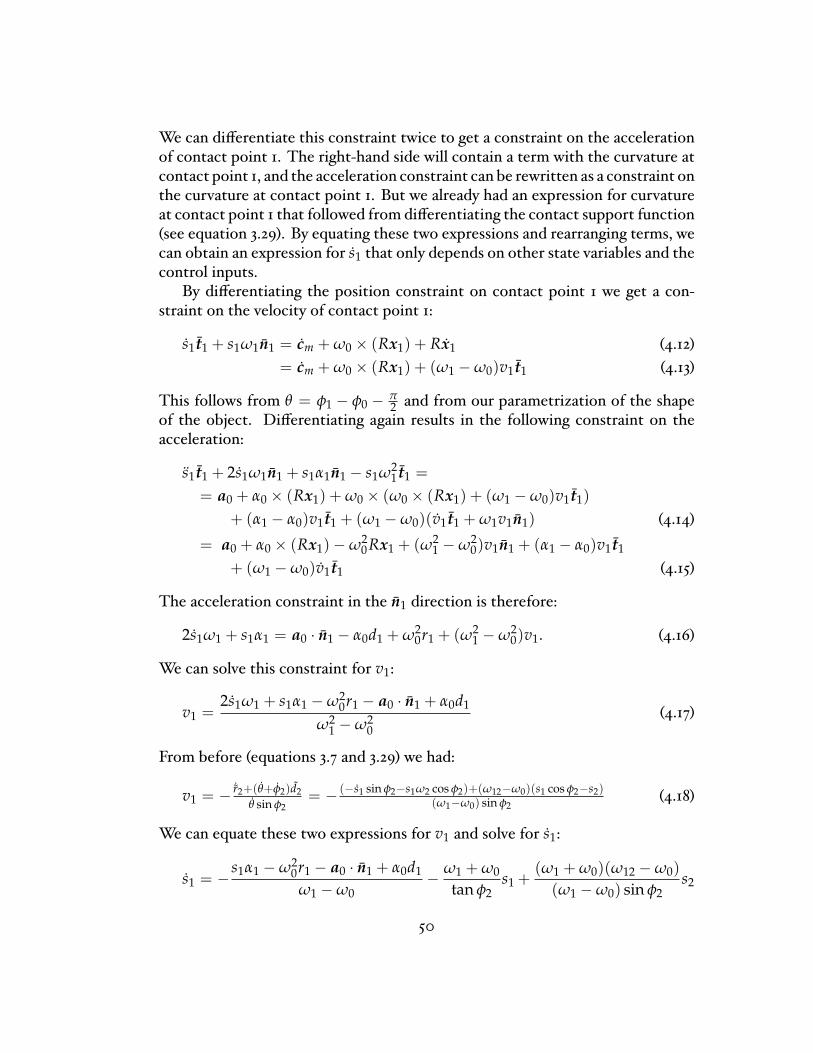
We can di�erentiate this constraint twice to get a constraint on the accelerationof contact point 1. The right-hand side will contain a term with the curvature atcontact point 1, and the acceleration constraint can be rewritten as a constraint onthe curvature at contact point 1. But we already had an expression for curvatureat contact point 1 that followed from di�erentiating the contact support function(see equation 3.29). By equating these two expressions and rearranging terms, wecan obtain an expression for s1 that only depends on other state variables and thecontrol inputs.By di�erentiating the position constraint on contact point 1 we get a con-

straint on the velocity of contact point 1:

s1t1 + s1ω1n1 = cm + ω0 × (Rx1) + Rx1 (4.12)= cm + ω0 × (Rx1) + (ω1 − ω0)v1t1 (4.13)

This follows from θ = φ1 − φ0 − π2 and from our parametrization of the shape

of the object. Di�erentiating again results in the following constraint on theacceleration:

s1t1 + 2s1ω1n1 + s1α1n1 − s1ω21 t1 =

= a0 + α0 × (Rx1) + ω0 × (ω0 × (Rx1) + (ω1 − ω0)v1t1)+ (α1 − α0)v1t1 + (ω1 − ω0)(v1t1 + ω1v1n1) (4.14)

= a0 + α0 × (Rx1)− ω20Rx1 + (ω2

1 − ω20)v1n1 + (α1 − α0)v1t1

+ (ω1 − ω0)v1t1 (4.15)

The acceleration constraint in the n1 direction is therefore:

2s1ω1 + s1α1 = a0 · n1 − α0d1 + ω20r1 + (ω2

1 − ω20)v1. (4.16)

We can solve this constraint for v1:

v1 =2s1ω1 + s1α1 − ω2

0r1 − a0 · n1 + α0d1

ω21 − ω2

0(4.17)

From before (equations 3.7 and 3.29) we had:

v1 = − ˙r2+(θ+φ2)d2θ sin φ2

= − (−s1 sin φ2−s1ω2 cos φ2)+(ω12−ω0)(s1 cos φ2−s2)(ω1−ω0) sin φ2

(4.18)

We can equate these two expressions for v1 and solve for s1:

s1 = −s1α1 − ω2

0r1 − a0 · n1 + α0d1

ω1 − ω0− ω1 + ω0

tan φ2s1 +

(ω1 + ω0)(ω12 − ω0)(ω1 − ω0) sin φ2

s2

50

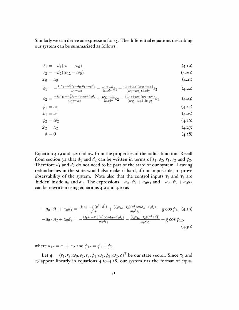
Similarly we can derive an expression for s2. The di�erential equations describingour system can be summarized as follows:

r1 = −d1(ω1 − ω0) (4.19)r2 = −d2(ω12 − ω0) (4.20)

ω0 = α0 (4.21)

s1 = − s1α1−ω20r1−a0·n1+α0d1ω1−ω0

− ω1+ω0tan φ2

s1 + (ω1+ω0)(ω12−ω0)(ω1−ω0) sin φ2

s2 (4.22)

s2 = −s2α12−ω20r2−a0·n2+α0d2

ω12−ω0+ ω12+ω0

tan φ2s2 − (ω12+ω0)(ω1−ω0)

(ω12−ω0) sin φ2s1 (4.23)

φ1 = ω1 (4.24)ω1 = α1 (4.25)φ2 = ω2 (4.26)ω2 = α2 (4.27)

ρ = 0 (4.28)

Equation 4.19 and 4.20 follow from the properties of the radius function. Recallfrom section 3.1 that d1 and d2 can be written in terms of s1, s2, r1, r2 and φ2.Therefore d1 and d2 do not need to be part of the state of our system. Leavingredundancies in the state would also make it hard, if not impossible, to proveobservability of the system. Note also that the control inputs τ1 and τ2 are`hidden' inside a0 and α0. The expressions −a0 · n1 + α0d1 and −a0 · n2 + α0d2can be rewritten using equations 4.9 and 4.10 as

−a0 · n1 + α0d1 = (I1α1−τ1)(ρ2+d21)

mρ2s1+ (I2α12−τ2)(ρ2 cos φ2−d1d2)

mρ2s2− g cos φ1, (4.29)

−a0 · n2 + α0d2 = − (I1α1−τ1)(ρ2 cos φ2−d1d2)mρ2s1

− (I2α12−τ2)(ρ2+d22)

mρ2s2+ g cos φ12,

(4.30)

where α12 = α1 + α2 and φ12 = φ1 + φ2.

Let q = (r1, r2, ω0, s1, s2, φ1, ω1, φ2, ω2, ρ)T be our state vector. Since τ1 andτ2 appear linearly in equations 4.19�4.28, our system �ts the format of equa-

51

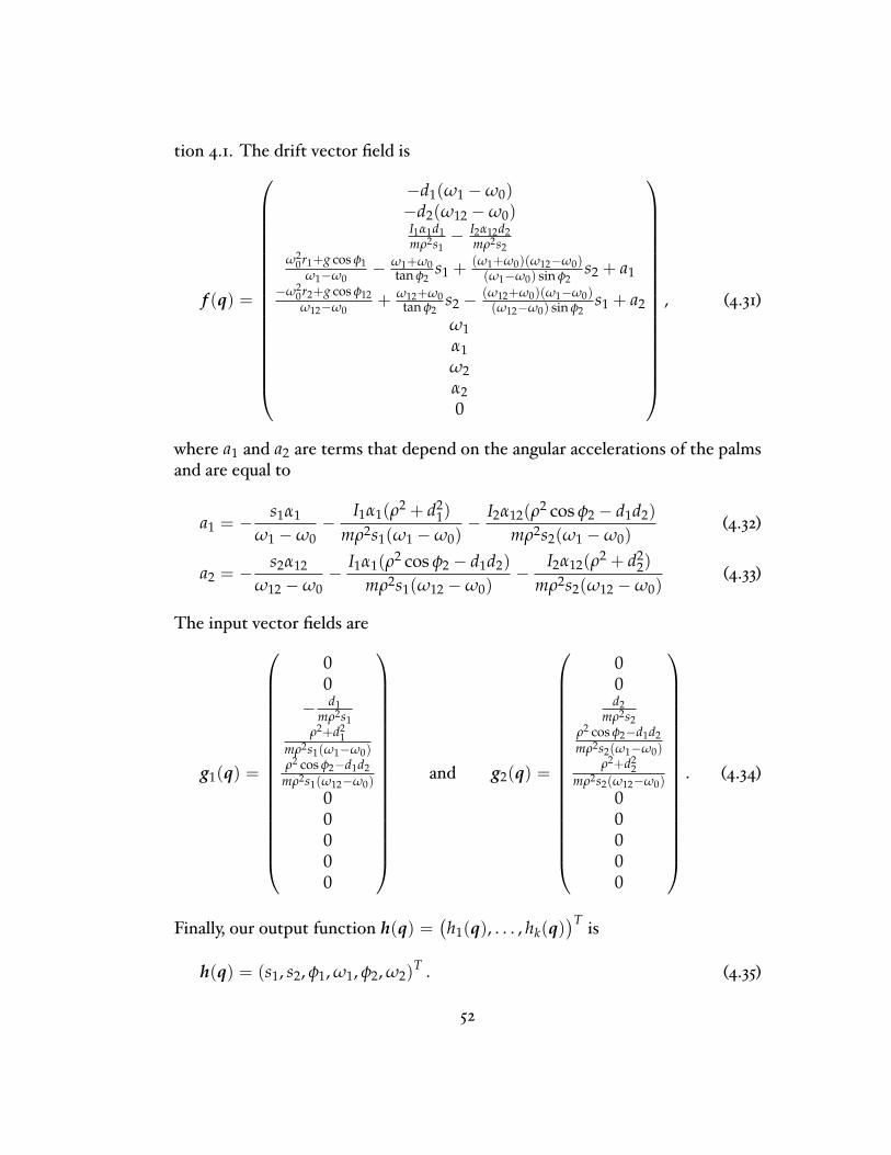
tion 4.1. The drift vector �eld is

f (q) =

−d1(ω1 − ω0)−d2(ω12 − ω0)I1α1d1mρ2s1

− I2α12d2mρ2s2

ω20r1+g cos φ1

ω1−ω0− ω1+ω0

tan φ2s1 + (ω1+ω0)(ω12−ω0)

(ω1−ω0) sin φ2s2 + a1

−ω20r2+g cos φ12ω12−ω0

+ ω12+ω0tan φ2

s2 − (ω12+ω0)(ω1−ω0)(ω12−ω0) sin φ2

s1 + a2

ω1α1ω2α20

, (4.31)

where a1 and a2 are terms that depend on the angular accelerations of the palmsand are equal to

a1 = − s1α1

ω1 − ω0−

I1α1(ρ2 + d21)

mρ2s1(ω1 − ω0)− I2α12(ρ2 cos φ2 − d1d2)

mρ2s2(ω1 − ω0)(4.32)

a2 = − s2α12

ω12 − ω0− I1α1(ρ2 cos φ2 − d1d2)

mρ2s1(ω12 − ω0)−

I2α12(ρ2 + d22)

mρ2s2(ω12 − ω0)(4.33)

The input vector �elds are

g1(q) =

00

− d1mρ2s1

ρ2+d21

mρ2s1(ω1−ω0)ρ2 cos φ2−d1d2

mρ2s1(ω12−ω0)00000

and g2(q) =

00d2

mρ2s2ρ2 cos φ2−d1d2mρ2s2(ω1−ω0)

ρ2+d22

mρ2s2(ω12−ω0)00000

. (4.34)

Finally, our output function h(q) =(h1(q), . . . , hk(q)

)T is

h(q) = (s1, s2, φ1, ω1, φ2, ω2)T . (4.35)

52

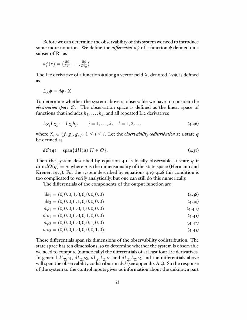
Before we can determine the observability of this systemwe need to introducesome more notation. We de�ne the di�erential dφ of a function φ de�ned on asubset of Rn as

dφ(x) =( ∂φ

∂x1, . . . , ∂φ

∂xn

)The Lie derivative of a function φ along a vector �eld X, denoted LXφ, is de�nedas

LXφ = dφ · X

To determine whether the system above is observable we have to consider theobservation space O. The observation space is de�ned as the linear space offunctions that includes h1, . . . , hk, and all repeated Lie derivatives

LX1 LX2 · · · LXl hj, j = 1, . . . , k, l = 1, 2, . . . (4.36)

where Xi ∈ { f , g1, g2}, 1 ≤ i ≤ l. Let the observability codistribution at a state qbe de�ned as

dO(q) = span{dH(q)|H ∈ O}. (4.37)

Then the system described by equation 4.1 is locally observable at state q ifdim dO(q) = n, where n is the dimensionality of the state space (Hermann andKrener, 1977). For the system described by equations 4.19�4.28 this condition istoo complicated to verify analytically, but one can still do this numerically.The di�erentials of the components of the output function are

ds1 = (0, 0, 0, 1, 0, 0, 0, 0, 0, 0) (4.38)ds2 = (0, 0, 0, 0, 1, 0, 0, 0, 0, 0) (4.39)dφ1 = (0, 0, 0, 0, 0, 1, 0, 0, 0, 0) (4.40)dω1 = (0, 0, 0, 0, 0, 0, 1, 0, 0, 0) (4.41)dφ2 = (0, 0, 0, 0, 0, 0, 0, 1, 0, 0) (4.42)dω2 = (0, 0, 0, 0, 0, 0, 0, 0, 1, 0). (4.43)

These di�erentials span six dimensions of the observability codistribution. Thestate space has ten dimensions, so to determine whether the system is observablewe need to compute (numerically) the di�erentials of at least four Lie derivatives.In general dLg1s1, dLg2s2, dLg1 Lg1s1 and dLg2 Lg2s2 and the di�erentials abovewill span the observability codistribution dO (see appendix A.2). So the responseof the system to the control inputs gives us information about the unknown part

53

of the state. We can use this information to improve the estimate for the valuesof the radius function at the contact points, the rotational velocity of the objectand its radius of gyration. Note that we can not use the vector �eld f , because wedo not have expressions for α1 and α2 in terms of the state variables and, hence,we can not compute the di�erentials of Lie derivatives along f .

The results above show that in general we will be able to observe the shape ofan unkown object. Moreover, the output function contains enough informationto recover a constant like the radius of gyration. This leads us to suspect that itmay be possible to recover another constant as well: the coe�cient of friction.Currently friction is not modeled, but we plan to address this in future work.

4.3 Moving the Palms at a Constant Rate

Although we have shown that the system in the previous section is observable,this does not directly translate to an actual observer. The observability tells usthat an observer exists, but constructing a well-behaved observer for a nonlinearsystem is nontrivial and is still an active area of research. Many observers (suchas those proposed by Gauthier et al. (1992) and Zimmer (1994)) rely on Liederivatives of the drift �eld. If we want to use such an observer we have toconstrain the motion of the palms by restricting them to move at a constant rate,i.e., α1 = α2 = 0. With this constraint the angular acceleration of the palmsvanishes and we do not have to compute derivatives of the accelerations withrespect to the state variables. Provided the palms are su�ciently sti� comparedto the object, we can easily realize this. Note that this is an assumption andthat in general a torque-based control system does not automatically translateto a velocity-based or position-based control system. For simplicity we will alsoassume that we already have recovered the radius of gyration.

Moving both palms at the same rate Suppose we move palm 1 and 2 at thesame rate. Then ω2 = 0, since it measures the relative rate of palm 2 to palm 1.Our state vector then reduces to q = (r1, r2, ω0, s1, s2, φ1)T. The angle betweenthe palms is constant, so φ2 does not need to be part of the state. For the samereason we can omit ω1 and ω2 from the state vector. The output function is now

54

h(q) = (s1, s2, φ1)T and the drift vector �eld simpli�es to

f (q) =

−d1(ω1 − ω0)−d2(ω1 − ω0)

0ω2

0r1+g cos φ1ω1−ω0

− (ω1 + ω0)d2/ sin φ2−ω2

0r2+g cos φ12ω1−ω0

+ (ω1 + ω0)d1/ sin φ2

ω1

. (4.44)

Recall from chapter 3, equation 3.7 that d1 = s2 cos φ2 − s1 and d2 = s1 cos φ2 −s2. We can compute the di�erentials and Lie derivatives that are necessary toprove the observability:

ds1 = (0, 0, 0, 1, 0, 0) (4.45)ds2 = (0, 0, 0, 0, 1, 0) (4.46)dφ1 = (0, 0, 0, 0, 0, 1) (4.47)

L f s1 = ds1 · f = ω20r1+g cos φ1

ω1−ω0+ (ω1 + ω0)(s2 − s1 cos φ2)/ sin φ2 (4.48)

dL f s1 =( ω2

0ω1−ω0

, 0, r1ω0(2ω1−ω0)+g cos φ1(ω1−ω0)2 + s2−s1 cos φ2

sin φ2, −ω1+ω0

tan φ2,

ω1+ω0sin φ2

, − g sin φ1ω1−ω0

)(4.49)

L f s2 =−ω2

0r2 + g cos φ12

ω1 − ω0+ (ω1 + ω0)(s2 cos φ2 − s1)/ sin φ2 (4.50)

dL f s2 =(0, −ω2

0ω1−ω0

, −r2ω0(2ω1−ω0)+g cos φ12(ω1−ω0)2 + s2 cos φ2−s1

sin φ2, −ω1+ω0

sin φ2,

ω1+ω0tan φ2

, − g sin φ12ω1−ω0

)(4.51)

L f L f s1 = −2ω20ω1(r1 cos φ2+r2)(ω1−ω0) sin φ2

− s1ω1(2ω0 + ω1)−g sin φ1(ω0+2ω1)

ω1−ω0(4.52)

dL f L f s1 =( −2ω2

0ω1(ω1−ω0) tan φ2

, −2ω20ω1

(ω1−ω0) sin φ2, −2ω0ω1(2ω1−ω0)(r1 cos φ2+r2)

(ω1−ω0)2 sin φ2− 2s1ω1

− 3ω1g sin φ1(ω1−ω0)2 , −ω1(2ω0 + ω1), 0, −g cos φ1(ω0+2ω1)

ω1−ω0

)(4.53)

It can be shown that the determinant of the matrix that has colums ds1, ds2,dφ1, dL f s1, dL f s2 and dL f L f s1 is equal to

gω40ω1 sin φ1

(ω1 − ω0)4 (4.54)

In other words, the system is observable as long asω0 andω1 are nonzero and notequal to each other. Recall from equation 3.28 that θ is equal toω1 −ω0. So ifω0

55

and ω1 are equal to each other, θ = 0 and we cannot observe the curvature at thecontact points (cf. equations 3.29 and 3.30). Note that the system is observablesolely in terms of the drift vector �eld.

Keeping one palm �xed Let us now consider the case ω1 = 0: palm 1 is�xed and palm 2 is moving at a constant rate. The state vector then reduces toq = (r1, r2, ω0, s1, s2, φ2)T. The output function is now h(q) = (s1, s2, φ2)T andthe drift vector �eld simpli�es to

f (q) =

d1ω0−d2(ω2 − ω0)

0

−ω20r1+g cos φ1

ω0− ω0s1

tan φ2− (ω2−ω0)s2

sin φ2−ω2

0r2+g cos φ12ω2−ω0

+ (ω2+ω0)s2tan φ2

+ (ω2+ω0)ω0s1(ω2−ω0) sin φ2

ω2

(4.55)

As before, we need to compute the di�erentials and Lie derivatives to determineobservability:

ds1 = (0, 0, 0, 1, 0, 0) (4.56)ds2 = (0, 0, 0, 0, 1, 0) (4.57)dφ2 = (0, 0, 0, 0, 0, 1) (4.58)

L f s2 = −ω20r1+g cos φ1

ω0− ω0s1

tan φ2− (ω2−ω0)s2

sin φ2(4.59)

dL f s1 =(− ω0, 0, −r1 + g cos φ1

ω20

− s1tan φ2

+ s2sin φ2

, − ω0tan φ2

, −ω2−ω0sin φ2

,

ω0s1+(ω2−ω0)s2 cos φ2sin2 φ2

)(4.60)

L f s2 = −ω20r2+g cos φ12

ω2−ω0+ (ω2+ω0)s2

tan φ2+ (ω2+ω0)ω0s1

(ω2−ω0) sin φ2(4.61)

dL f s2 =(0, −ω2

0ω2−ω0

, −r2ω0(2ω2−ω0)+g cos φ12(ω2−ω0)2 + s2

tan φ2− s1(ω2

2+2ω0ω2−ω20)

(ω2−ω0)2 sin φ2,

(ω2+ω0)ω0(ω2−ω0) sin φ2

, ω2+ω0tan φ2

, −g sin φ12ω2−ω0

− s2(ω2+ω0)sin2 φ2

− (ω2+ω0)ω0s1 cos φ2(ω2−ω0) sin2 φ2

)(4.62)

L f L f s2 = −2ω20ω2(r1+r2 cos φ2)(ω2−ω0) sin φ2

− s2ω2(2ω0 + ω2)−g(ω0+2ω2) sin φ12

ω2−ω0(4.63)

dL f L f s2 =( −2ω2

0ω2(ω2−ω0) sin φ2

, −2ω20ω2

(ω2−ω0) tan φ2, −2ω0ω2(2ω2−ω0)(r1+r2 cos φ2)

(ω2−ω0)2 sin φ2− 2s2ω2

− 3ω2g sin φ12(ω2−ω0)2 , 0,−ω2(2ω0 + ω2), 2ω2

0ω2(r1 cos φ2+r2)(ω2−ω0) sin2 φ2

− −g cos φ12(ω0+2ω2)ω2−ω0

)(4.64)

56

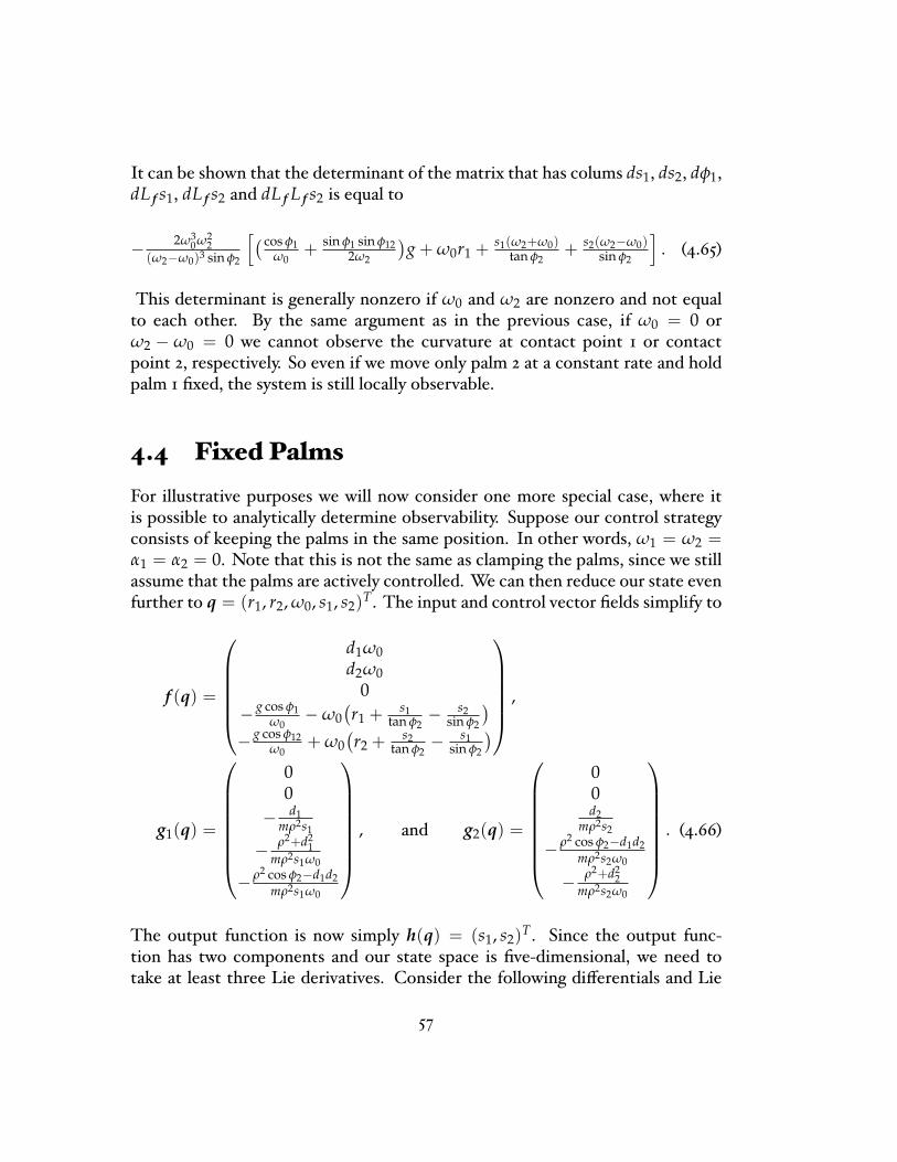
It can be shown that the determinant of the matrix that has colums ds1, ds2, dφ1,dL f s1, dL f s2 and dL f L f s2 is equal to

− 2ω30ω2

2(ω2−ω0)3 sin φ2

[( cos φ1ω0

+ sin φ1 sin φ122ω2

)g + ω0r1 + s1(ω2+ω0)

tan φ2+ s2(ω2−ω0)

sin φ2

]. (4.65)

This determinant is generally nonzero if ω0 and ω2 are nonzero and not equalto each other. By the same argument as in the previous case, if ω0 = 0 orω2 − ω0 = 0 we cannot observe the curvature at contact point 1 or contactpoint 2, respectively. So even if we move only palm 2 at a constant rate and holdpalm 1 �xed, the system is still locally observable.

4.4 Fixed PalmsFor illustrative purposes we will now consider one more special case, where itis possible to analytically determine observability. Suppose our control strategyconsists of keeping the palms in the same position. In other words, ω1 = ω2 =α1 = α2 = 0. Note that this is not the same as clamping the palms, since we stillassume that the palms are actively controlled. We can then reduce our state evenfurther to q = (r1, r2, ω0, s1, s2)T. The input and control vector �elds simplify to

f (q) =

d1ω0d2ω0

0− g cos φ1

ω0− ω0

(r1 + s1

tan φ2− s2

sin φ2

)− g cos φ12

ω0+ ω0

(r2 + s2

tan φ2− s1

sin φ2

)

,

g1(q) =

00

− d1mρ2s1

− ρ2+d21

mρ2s1ω0

− ρ2 cos φ2−d1d2mρ2s1ω0

, and g2(q) =

00d2

mρ2s2

− ρ2 cos φ2−d1d2mρ2s2ω0

− ρ2+d22

mρ2s2ω0

. (4.66)

The output function is now simply h(q) = (s1, s2)T. Since the output func-tion has two components and our state space is �ve-dimensional, we need totake at least three Lie derivatives. Consider the following di�erentials and Lie

57

derivatives:

ds1 = (0, 0, 0, 1, 0) (4.67)ds2 = (0, 0, 0, 0, 1) (4.68)

L f s1 = − g cos φ1ω0

− ω0(r1 + s1

tan φ2− s2

sin φ2

)(4.69)

dL f s1 =(− ω0, 0, g cos φ1

ω20

−(r1 + s1

tan φ2− s2

sin φ2

),− ω0

tan φ2, ω0

sin φ2

)(4.70)

L f s2 = − g cos φ12ω0

− ω0(r2 + s2

tan φ2− s1

sin φ2

)(4.71)

dL f s2 =(

0,−ω0,− g cos φ12ω2

0−(r2 + s2

tan φ2− s1

sin φ2

), ω0

sin φ2,− ω0

tan φ2

)(4.72)

L f L f s1 = ω20(−d1 + r1

tan φ2+ r2

sin φ2− s1) + g sin φ1 = g sin φ1 (4.73)

dL f L f s1 = (0, 0, 0, 0, 0) (4.74)

The step in equation 4.73 follows from expression 3.18. Because of symmetrydL f L f s2 is equal to the 0 vector as well. This means that with �xed palms thesystem is not observable in terms of just the drift �eld f . Now suppose wecompute the Lie derivative of s1 along g1 and its di�erential:

Lg1s1 = −ρ2 + d2

1mρ2s1ω0

(4.75)

dLg1s1 = 1mρ2s1ω0

( −2d1tan φ2

, −2d1sin φ2

, ρ2+d21

ω0, 2d1 + ρ2+d2

1s1

, 0)

(4.76)

Thedi�erentials ds1, ds2, dL f s1, dL f s2 and dLg1s1 generally span the observabilitycodistribution and, hence, the system is observable. It is important to rememberthat the palms are actively controlled, i.e., the palms are not clamped. Otherwisewe would not know the torques exerted by the palms. We need the torquesto integrate (by using an observer) the di�erential equation 4.1. As mentionedbefore, the construction of an observer that relies on the control vector �elds isnontrivial. Since the motion of the palms is so constrained, the system is likelyto observe only a small fraction of an unknown shape. Therefore we suspect thatif one were to construct an observer it would have very limited practical value.

4.5 AnObserver Based onNewton'sMethodThe observer we implemented is based on Newton's method (Zimmer, 1994) for�nding the roots (i.e., zeros) of a function. Before we describe the details of ourobserver, let us �rst quickly review Newton's method. Suppose we want to �nda root of a function f : R → R. Let x0 be an initial guess close to a root x of f .

58

xx0

yy=f(x)

x1x2x

Figure 4.2: Newton's method.

Then the sequence xn+1 = xn − f (xn)f ′(xn) , n ≥ 0, converges quadratically to x. See

�gure 4.2 for an illustration of this method.With an observer we are trying to minimize the di�erence between the state

estimate and the true state. We cannot actually observe the true state, but wecan consider the di�erences between the expected output based on the estimateand the actual output. Following Zimmer, we say that a system in the form ofequations 4.1�4.2 is strongly observable in Q if and only if for any time intervalI = [0, T] and for any given initial states q1(0), q2(0) ∈ Q and for any t ∈ I

� the states q1(t) and q2(t) remain in Q, and� the system outputs y(q1(t)) and y(q2(t)) are identical in I only if q1 = q2.

A system is called locally strongly observable in Q if and only if there is an ε > 0 sothat for every t in the time interval I = [0, T] and for every q ∈ Q the system attime t is locally observable in Bε(q) ∩ Q, where Bε(q) is a n-dimensional spherewith radius ε centered at q.Let us now de�ne the distance function k : Rn ×Rn → R+:

k(q1(0), q2(0)) = 12

∫ T

0‖h(q1(t))− h(q2(t))‖2dt (4.77)

So the distance between two states q1 and q2 at t = 0 is de�ned as the di�erencebetween the outputs over time T obtained by integrating out equation 4.1 foreach state and applying the output function to it. So we can transform the stateestimation problem into aminimization problem. Let q∗ be an estimate for q andlet kq = k(·, q) be the error function for a particular state. Clearly, if a system isstrongly observable, then kq has a unique minimum at q, equal to 0. But q is alsoa root of the �rst derivative of kq. We can apply Newton's method to improve

59

the state estimate q∗ of q:

q∗new = q∗old −

(∂2kq

(∂q)2

)−1 (∂kq

∂q

)T

(4.78)

(The `T' denotes transpose here, not time.) Note that to evaluate kq(q∗) we donot need to know q. All we need is the output over an interval I. For this methodto be successful a number of conditions need to be satis�ed:

� The function kq needs to be convex near q. This is equivalent to sayingthat the Hessian matrix ∂2kq

(∂q)2 is positive de�nite. Zimmer showed that thisis the case if and only if the linearized system around q is locally observablein I.

� This Hessian matrix also has to be invertible. Zimmer derived su�cientconditions to test if that is the case.

If these conditions are not satis�ed (for instance, near or at singularities), we needto resort to other methods for shape recovery. The simplest method is to simplyintegrate the di�erential equations describing our system. Alternatively, we canignore the sensor data while the above conditions are not satis�ed and restartour observer when they are.There are several ways we can use the update rule of equation 4.78 in an

observer depending on the amount of computation we are willing to spend onimproving the state estimate. If we are trying to reconstruct a shape in real-time, then we may not be able to take many Newton steps. In that case, wecan update our state estimate every T seconds by taking one Newton step asgiven by equation 4.78. If we are reconstructing the shape o�ine, we can takean arbitrary number of Newton steps. We could even update the state estimatemore frequently than every T seconds.Although most observers are used for online state estimation, this Newton

observer has more of an o�ine �avor. There is a minimal delay of T secondsbetween measuring the output of the system and being able to correct the stateestimate of the system at that time, because the observer needs to know how anerror in the state estimate at a given time a�ects the output in the T secondsafter it.

4.6 SimulationResultsThe observer described above has been implemented in Matlab. The results ofone simulation are shown in �gures 4.3 and 4.4. We simulated the motion of a

60

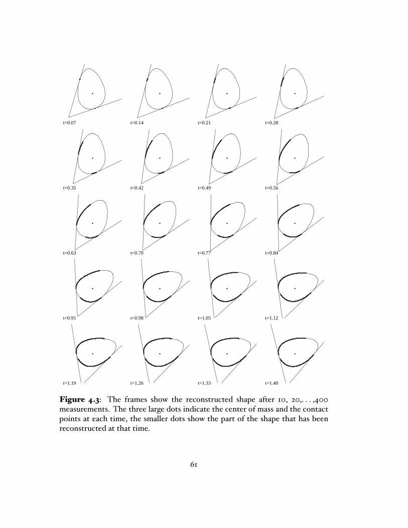
t=0.07 t=0.14 t=0.21 t=0.28

t=0.35 t=0.42 t=0.49 t=0.56

t=0.63 t=0.70 t=0.77 t=0.84

t=0.91 t=0.98 t=1.05 t=1.12

t=1.19 t=1.26 t=1.33 t=1.40

Figure 4.3: The frames show the reconstructed shape after 10, 20,. . . ,400measurements. The three large dots indicate the center of mass and the contactpoints at each time, the smaller dots show the part of the shape that has beenreconstructed at that time.

61

−1 0 1 2−2

−1.5

−1

−0.5

0

0.5

1

1.5

2

(a) The reconstructed shape0 0.2 0.4 0.6 0.8 1 1.2 1.4

−1.5

−1

−0.5

0

0.5

1

1.5

2

2.5

← initial guess for r1 and r

2

observed r1

observed r2

observed φ0

(b) The reconstructed radius function andorientation

0 0.2 0.4 0.6 0.8 1 1.2 1.4−10

−8

−6

−4

−2

0

2

4

6

8x 10

−4

error in r1

error in r2

error in φ0

(c) The absolute error in the radius func-tion and the orientation

0 0.2 0.4 0.6 0.8 1 1.2 1.4−1

0

1x 10

−4

error in s1

error in s2

error in φ1

(d) The absolute error in the sensor valuesand palm angle 1

Figure 4.4: Shape reconstruction with an observer based on Newton's method.

random smooth shape over 1.4 seconds. We split the total time into 400 timesteps and applied �ve Newton steps after every 80 time steps. At t = 0 we dosomething slightly di�erent. We assume the object's initial velocity is equal to0. This simpli�es the search for the initial conditions since we now only have tosearch for the initial values of the radius function at the contact points. The initialguess for the value of the radius function was set to 2 for both contact points.The initial value of ω0 is `clamped' to 0 at t = 0; the Newton observer cannotchange this initial value. After �ve Newton steps the observer has found valuesfor the radius function that are very close to the actual values. The recoveredvalues of the radius function are very close to the true values. Figure 4.4(d) shows

62

the di�erence in the sensor values the observer expected to see and the actualsensor values.

4.7 Arbitrary PalmShapesIn this chapter we wrote the shape and motion of the object as a function of theshape and motion of the palms. Instead of the shape and motion of the palms,we could also use the contact point positions and velocities in world coordinates.Let ci be contact point i in world coordinates. Then there exist functions Cpalmsand Cobject such that

Cpalms(τ1, φ1, ω1, s1, s1, τ2, φ2, ω2, s2, s2) =(c1, c1, c2, c2

)T (4.79)

Cobject(r1, r1, r2, r2, φ0, ω0, α0, a0) =(c1, c1, c2, c2

)T (4.80)

E�ectively, we have used world coordinates to decouple the solution for the shapeand motion of the unknown object from the shape and motion of the palm. Thisallows us to use di�erently shaped palms without changing the solution for theshape and motion of the unknown object. Suppose we were to use circular palms.(For di�erent palm shapes the approach would be the same.) Let c1 and c2 bede�ned as

c1 = b1R1

(sin(s1/b1)

1− cos(s1/b1)

)(4.81)

c2 = b2R2

(sin(s2/b2)

cos(s2/b2)− 1

)(4.82)

Here bi is the radius of palm i and Ri a rotation matrix equal to

Ri =(

cos φi − sin φisin φi cos φi

).

Note that φ2 is now the angle between the X-axis and palm 2, and not the anglebetween the palms. The sensor values correspond to arc length. See �gure 4.5for an illustration. Note that just as with �at palms, if si = 0, then ci = 0. Infact, in the limit, as b1 and b2 approach in�nity, the circular palms are equivalentto the �at palms.The local coordinate frames at the contact points are now

t1 = R1

(cos(s1/b1)sin(s1/b1)

)t2 = R2

(− cos(s2/b2)

sin(s2/b2)

)n1 = R1

(− sin(s1/b1)cos(s1/b1)

)n2 = −R2

(sin(s2/b2)cos(s2/b2)

)

63

palm 1

palm 2

φ1

s1s2

c1c2

b1

Figure 4.5: Circular palms.

By looking at projections of ci onto these frames we can again obtain a systemof di�erential equations similar to equations 4.19�4.28. Most of the di�erentialequations remain the same. The ones that depend directly on the palm shapeare the equations for ω0, s1, and s2. Below we outline the procedure for provingobservability for a system with circular palms.The �rst and second derivative of contact point 1 are:

c1 = ω1 × c1 + s1t1 (4.83)c1 = α1 × c1 + ω1 × (ω1 × c1 + 2s1t1) + s1t1 + (s2

1/b1)n1

= α1 × c1 − ω21c1 + 2ω1s1n1 + s1t1 + (s2

1/b1)n1 (4.84)

We can write c1 also as a function of the pose of the object: c1 = cm + R0x1.By di�erentiating this expression twice and equating it to expression 4.84, weobtain a constraint on the acceleration at contact point 1. In fact, we alreadycomputed the second derivative of this expression; it is given by the right-handside of equation 4.15. The projection of the acceleration constraint onto the palmnormal at contact point 1 is given by

α1(c1 · t1)− ω21(c1 · n1) + 2ω1s1 + s2

1/b1

= a0 · n1 + ω20r1 − α0d1 + (ω2

1 − ω20)v1. (4.85)

64

Solving for v1 we get:

v1 = α1(c1·t1)−ω21(c1·n1)+2ω1 s1+s2

1/b1−ω20r1−a0·n1+α0d1

ω21−ω2

0(4.86)

= α1b1 sin(s1/b1)−ω21b1(cos(s1/b1)−1)+2ω1 s1+s2

1/b1−ω20r1−a0·n1+α0d1

ω21−ω2

0(4.87)

The expression we obtained for v1 in chapter 3, equation 3.29, is still valid if wereplace φ2 with the time derivative of the angle between t1 and −t2. The gener-alized support functions can still be expressed as functions of the sensor valuesand palm angles, but these expressions will now be very di�erent. We can equateequation 3.29 and 4.86, substitute the expressions for the generalized radius func-tions corresponding to spherical palms, and solve for s1. Since equation 3.29 islinear in s1 and equation 4.86 quadratic in s1, there exist potentially two solutionsfor s1. Since we assume the object is convex, we have the constraint v1 > 0. Thisallows us to reject solutions for s1 that make v1 negative. In a similar manner wecan obtain a solution for s2.The dynamics of a system with circular palms are almost the same as be-

fore. The only di�erence is that the moment arm for the moment of contactforce i around the origin is no longer equal to si. The palm dynamics are now(cf. equations 4.7 and 4.8):

I1α1 = τ1 − fc1(c1 · t1) = τ1 − fc1b1 sin(s1/b1) (4.88)I2α12 = τ2 − fc2(c2 · t2) = τ2 + fc2b2 sin(s2/b2) (4.89)

The solutions for a0 and α0 are therefore (cf. equations 4.9 and 4.10):

a0 = − I1α1 − τ1

mb1 sin(s1/b1)n1 +

I2α12 − τ2

mb2 sin(s2/b2)n2 + g (4.90)

α0 =I1α1 − τ1

mρ2b1 sin(s1/b1)d1 −

I2α12 − τ2

mρ2b2 sin(s2/b2)d2 (4.91)

By de�nition, ω0 = α0, but we also need these solutions for the solution of s1 ands2. Proving observability given these solutions is rather cumbersome, due to thenonlinearity of the palms. We plan to implement this model in future work. Inthis implementation we will check for observability numerically. It seems likelythat the system is observable for most combinations of b1 and b2. So we may beable to choose the radii of the palms such that the system is observable.

Discussion Changing the palm shapes raises many new questions. Intuitively,it seems that circular palms would be `better' than �at palms, but can we quantify

65

this? It also seems that with circular palms we would have to move the palms lessto reach a point on the surface.Suppose the palms are actually deformable, in a controlled way, by varying

bi. By reducing bi from ∞ to 0 while maintaining the same tangent plane at thecontact point we can probe the local curvature without having tomove the shape.For this approach to work the palms need to be small enough to avoid collisionswith parts of the shape that are not in a small neighborhood around the contactpoint. We think it will be interesting to �nd out how these enveloping graspscan be used if the palms are not small and if the contact points do change whilethe object is enveloped.

66

C h a p t e r 5

Shape Reconstructionin Three Dimensions

Naturally we would like to extend the results from the previous chapters to threedimensions. We can manipulate an object with three planar palms as shown in�gure 1.2. Although the same general approach can also be used for the 3D case,there are also some fundamental di�erences. First of all, the di�erence is notjust one extra dimension, but three extra dimensions: a planar object has threedegrees of freedom and a 3D object has six. Analogous to the planar case we canderive a constraint on the position of the center of mass if we assume quasistaticdynamics. This constraint gives us the X and Y coordinate of the center of mass(see appendix A.3). However, assuming quasistatic dynamics is not su�cient tosolve for the motion of an unknown object: if the object stays in contact with thepalms it has three degrees of freedom, but the quasistatic dynamics give us onlytwo constraints. Another di�erence from the planar case is that in 3D we cannotcompletely recover an unknown shape in �nite time, since the contact points traceout only curves on the surface of the shape.

5.1 NotationIn 3D the surface of an arbitrary smooth convex object can be parameterizedwith spherical coordinates θ = (θ1, θ2) ∈ [0, 2π) × [−π

2 , π2 ]. For a given θ we

de�ne the following right-handed coordinate frame

t1(θ) =

− sin θ1cos θ1

0

(5.1)

67

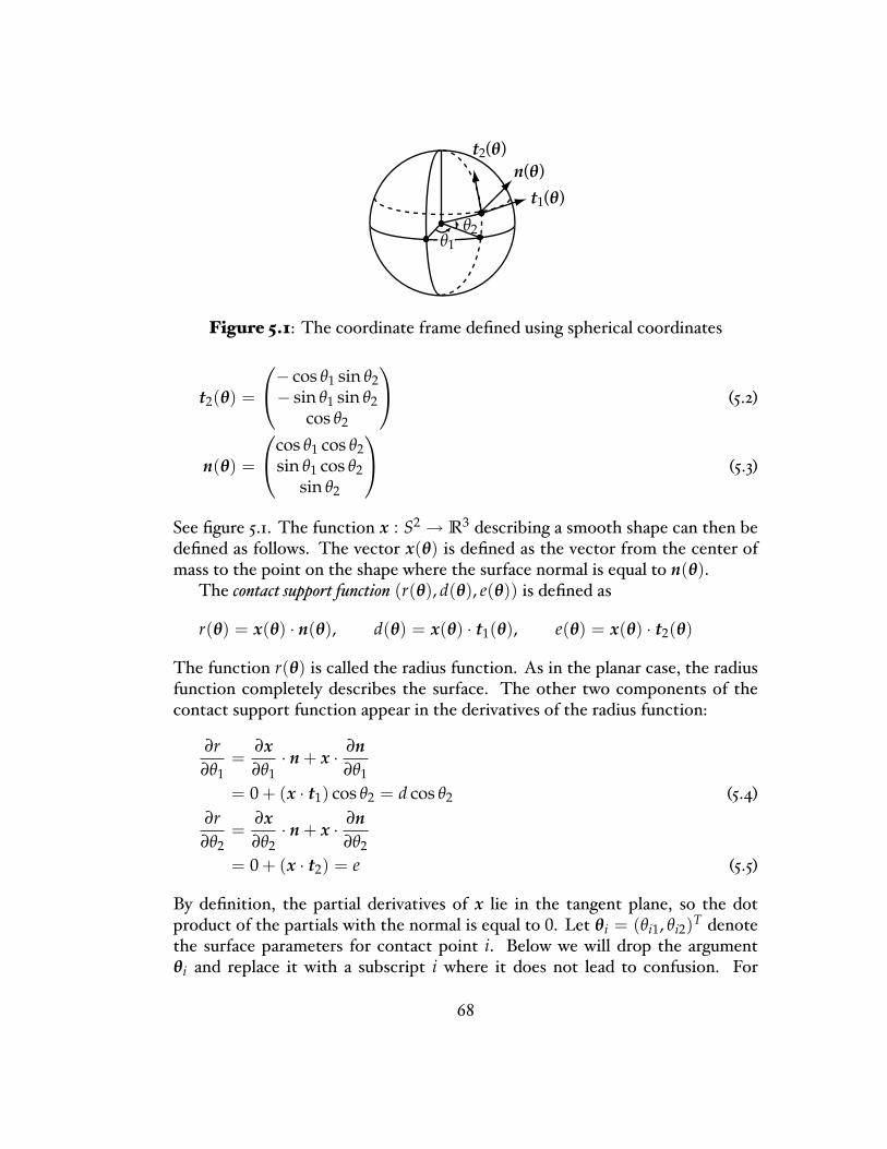
Figure 5.1: The coordinate frame de�ned using spherical coordinates

t2(θ) =

− cos θ1 sin θ2− sin θ1 sin θ2

cos θ2

(5.2)

n(θ) =

cos θ1 cos θ2sin θ1 cos θ2

sin θ2

(5.3)

See �gure 5.1. The function x : S2 → R3 describing a smooth shape can then bede�ned as follows. The vector x(θ) is de�ned as the vector from the center ofmass to the point on the shape where the surface normal is equal to n(θ).The contact support function (r(θ), d(θ), e(θ)) is de�ned as

r(θ) = x(θ) · n(θ), d(θ) = x(θ) · t1(θ), e(θ) = x(θ) · t2(θ)

The function r(θ) is called the radius function. As in the planar case, the radiusfunction completely describes the surface. The other two components of thecontact support function appear in the derivatives of the radius function:

∂r∂θ1

=∂x∂θ1

· n + x · ∂n∂θ1

= 0 + (x · t1) cos θ2 = d cos θ2 (5.4)∂r∂θ2

=∂x∂θ2

· n + x · ∂n∂θ2

= 0 + (x · t2) = e (5.5)

By de�nition, the partial derivatives of x lie in the tangent plane, so the dotproduct of the partials with the normal is equal to 0. Let θi = (θi1, θi2)T denotethe surface parameters for contact point i. Below we will drop the argumentθi and replace it with a subscript i where it does not lead to confusion. For

68

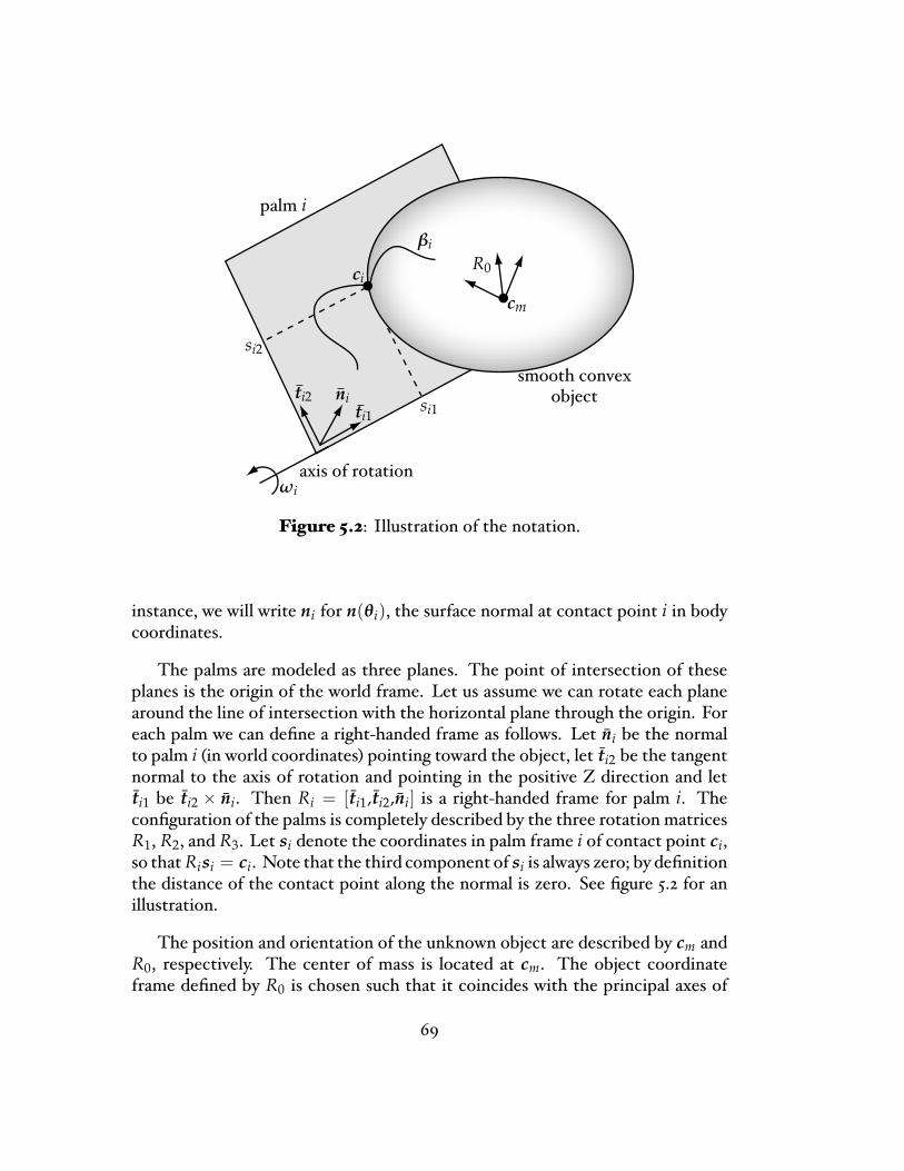
Figure 5.2: Illustration of the notation.

instance, we will write ni for n(θi), the surface normal at contact point i in bodycoordinates.

The palms are modeled as three planes. The point of intersection of theseplanes is the origin of the world frame. Let us assume we can rotate each planearound the line of intersection with the horizontal plane through the origin. Foreach palm we can de�ne a right-handed frame as follows. Let ni be the normalto palm i (in world coordinates) pointing toward the object, let ti2 be the tangentnormal to the axis of rotation and pointing in the positive Z direction and letti1 be ti2 × ni. Then Ri = [ti1,ti2,ni] is a right-handed frame for palm i. Thecon�guration of the palms is completely described by the three rotation matricesR1, R2, and R3. Let si denote the coordinates in palm frame i of contact point ci,so thatRisi = ci. Note that the third component of si is always zero; by de�nitionthe distance of the contact point along the normal is zero. See �gure 5.2 for anillustration.

The position and orientation of the unknown object are described by cm andR0, respectively. The center of mass is located at cm. The object coordinateframe de�ned by R0 is chosen such that it coincides with the principal axes of

69

inertia. The inertia matrix I can then be written as

I = m

ρ2x 0 0

0 ρ2y 0

0 0 ρ2z

,

where m is the mass of the object, and the ρ's correspond to the radii of gyration.We will write βi for the curve traced out on the surface of the object by contactpoint i. So βi(t) = x

(θi(t)

).

5.2 Local ShapeWe can recover the local shape at the contact points by considering the distancesbetween the contact points and the rates at which they change. We can writethe constraint that the object maintains contact with each palm as

ci = cm + R0βi, i = 1, 2, 3 (5.6)

The velocity of contact point i is therefore

ci = cm + ω0 × R0βi + R0βi (5.7)

The di�erence between two contact point velocities is

ci − cj = ω0 × R0(βi − β j) + R0(βi − β j) (5.8)= ω0 × (ci − cj) + R0(βi − β j) (5.9)

Since we assume the object is smooth, we have that ni · βi = 0. Furthermore,the palm normals and object are related by the object orientation matrix:

ni = −R0ni (5.10)

since ni is in world coordinates and ni is in object coordinates. We can combinethese constraints to solve for βi:

ni · R0βi = 0 (5.11)nj · R0βi = nj ·

(ci − cj − ω0 × (ci − cj)

)(5.12)

nk · R0βi = nk ·(ci − ck − ω0 × (ci − ck)

), (5.13)

such that i, j, and k are distinct. Let Q be the de�ned as the 3 × 3 matrix withentries qji:

qji = nj ·(ci − cj − ω0 × (ci − cj)

)(5.14)

Then we can write the solution for β1, β2, and β3 more compactly as

70

(β1 β2 β3

)= B−1Q, (5.15)

where B =(n1 n2 n3

)T R0. As long as the palms are in general position, B willbe invertible. Equation 5.15 describes the curves traced out by the contact pointson the surface of the object (in body coordinates) as a function of the motionof the palms, the sensor values and the motion of the object. Note that thesecurves are not independent of each other. We know the con�gurations of thepalms and the sensor values. If we also know one of the curves and the motionof the object, we can reconstruct the other curves. Below we will show that wecan reconstruct all three curves by solving for the values of the radius functionalong the curves. Using equations 5.4 and 5.5, the derivative with respect to timeof the radius function at contact point i is

ri =∂r

∂θi1θi1 +

∂r∂θi2

θi2 =(

di cos θi2ei

)· θi (5.16)

We will rewrite the right-hand side of this equation as a function of the motionof the palms and the object, and the values of the radius function at the contactpoints. Using the position constraints we can rewrite di and ei as a function ofthe con�guration of the palms and ri. We can write βi as

βi = rini + diti1 + eti2 (5.17)

The vector between contact point i and contact point j is then

ci − cj = R0(βi − β j) = R0(rini + diti1 + eti2 − rjnj + djtj1 + etj2) (5.18)

By rearranging terms we can obtain the following solution for the d's and e's:d1e1d2e2d3e3

=

t11 t12 −t21 −t22

000

000

t11 t12

000

000

−t31 −t32

−1

(RT

0 (c1 − c2)− (r1n1 − r2n2)

RT0 (c1 − c3)− (r1n1 − r3n3)

)

(5.19)

`Hidden' in the tangent vectors are the θi's. Using equation 5.3 we can write θi asa function of the palm surface normal ni:

θi =(

arctan(ni2, ni1)arcsin ni3

)(5.20)

71

The relationship between the normal ni and the orientations of the palms andobject is given by equation 5.10. The expression for ri also contains θi. Byconsidering the derivative of the normal ni we can obtain simple expressions forθi. On the one hand we have that

ni =∂n

∂θi1θi1 +

∂n∂θi2

θi2 = θi1 cos θ2ti1 + θi2ti2. (5.21)

But we can also obtain ni by di�erentiating equation 5.10:

ωi × ni = ˙ni = −ω0 × R0ni − R0ni ⇒ ni = RT0((ω0 − ωi)× ni

)(5.22)

Here ωi is the rotational velocity of palm i. Combining these two expressionsfor ni we can write θi as

θi =(ti1/ cos θi2 ti2

)T RT0((ω0 − ωi)× ni

)(5.23)

Let us now consider the constraints on the acceleration of the object inducedby the three point contact assumption. This will provide us with an additionalconstraint on βi and will give us some more insight into how the 3D case isfundamentally di�erent from the planar case. By di�erentiating equation 5.7 weobtain the following constraint on the acceleration:

ci = a0 + α0 × R0βi + ω0 × (ω0 × R0βi + 2R0βi) + R0βi, (5.24)

where a0 and α0 are the acceleration and angular acceleration of the object. (Wewill solve for a0 and α0 in the next section by analyzing the dynamics.) Observethat from di�erentiation of the smoothness constraint βi · ni = 0 it follows thatβi · ni = −βi · ni. We can therefore rewrite the acceleration constraint in thenormal direction as a constraint on βi. First, we rewrite the terms containing βiand βi:

ni · (ω0 × 2R0βi) + ni · R0βi = 2(ni × ω0) · R0βi + R0(ni · βi)

= 2(ni × ω0) · R0βi + ((ω0 − ωi)× ni) · R0βi

= (ni × (ω0 + ωi)) · R0βi

The constraint on βi is therefore

(ni × (ω0 + ωi)) · R0βi = ni ·(ci − a0 − α0 × R0βi − ω0 × (ω0 × R0βi)

)(5.25)

72

Let us now consider what how the acceleration constraint describes certaintime-independent shape properties of the contact curves. TheDarboux frame�eld(Spivak, 1999b) can be used to describe curves on a surface. For the curve βi theDarboux frame �eld is de�ned by the unit tangent T of βi, the surface normal Urestricted to βi, and V = U × T. The normalU coincides with ni. Note that thenormal of the curve does not necessarily coincide with the normal of the surface.Similar to the Frenet frame �eld, the derivatives of T, V, andU can be expressedin terms of T, V, and U:

T = v( κgV + κnU) (5.26)V = v(−κgT + τgU ) (5.27)U = v(−κnT−τgV ) (5.28)

Here v = ‖βi‖ is the velocity of the curve, κg the geodesic curvature, κn the normalcurvature, and τg the geodesic torsion. The geodesic curvature at a point describesthe `bending' of the curve in the tangent plane of the surface at that point. Thenormal curvature at a point describes the `bending' of the curve in the surfacenormal direction. Using this frame �eld we can write βi as

βi = vT + vT = vT + v2(κgV + κnU) (5.29)

So by taking the dot product with the normal on both sides of the accelerationconstraint we can obtain a constraint on the normal curvature κn of the curve:

κn = βi ·U = βi · ni = −βi · ni (5.30)

On the right-hand sidewe can substitute the solutions fromequations 5.15 and 5.22for βi and ni, respectively. In the planar case the velocity of the curve is equal tothe radius of curvature, and the acceleration constraint determines the (normal)curvature at the contact points. In the 3D case, the acceleration constraintputs a constraint on the normal curvature at the contact points. But now wehave two extra curve shape parameters, κg and τg, which are equal to zeroin the planar case. In other words, in 3D the contact point curves are lessconstrained than in 2D. Let the state of the system in 3D be de�ned as q =(r1, r2, r3, R0, ω0, s1, s2, s3, φ1, φ2, φ3)T, where φi is the angle between palm i andthe X-Y plane. Then having fewer constraints in 3D means that we cannot writethe behavior of the system in state-space form q = f (q, u), where u is a vectorof control inputs. More speci�cally, we can not write si as a function of statevariables and controls.

73

5.3 DynamicsThe solution for the shape of the object depends on themotion of the object. Wecan solve for the motion by writing out the dynamics equations for the systemformed by the palms and the object. Let Ii be the moment of inertia of palm iaround its axis of rotation, αi the angular acceleration around that axis, τi thetorque produced by palm i's motor at the axis of rotation, and fi the magnitudeof the contact force. Then the motion of palm i is described by

Iiαi = τi − fisi2, (5.31)where si2 is the second component of si. From the de�nition of the palm frame itfollows that si2 measures the distance to the axis of rotation (see also �gure 5.2).The net force and net torque on the object are given by Newton's and Euler'sequations:

F0 = ma0 = Fg +3

∑i=1

fini (5.32)

τ0 = I ′α0 + ω0 × I ′ω0 =3

∑i=1

τci (5.33)

where

I ′ = R0IRT0 (5.34)

τci = (R0βi)× ( fini) = − fiR0(βi × ni) (5.35)From these equations we can solve for the angular acceleration of the object, α0:

α0 = −I ′−1(ω0 × I ′ω0 +3

∑i=1

τi − Iiαi

si2R0(βi × ni)

)(5.36)

Let us assume we can control the palms to move at a constant rotational velocity.The angular acceleration terms αi will then disappear. We can summarize thesimultaneous solution for the shape and motion of an unknown smooth convexobject manipulated by three �at palms with the following system of di�erentialequations:

ri = (di cos θi2, ei)T · θi, i = 1, 2, 3 (5.37)R0 = ω0R0 (5.38)

ω0 = −I ′−1(ω0 × I ′ω0 +3

∑i=1

τi

si2R0(βi × ni)

)(5.39)

74

Here ω0 is the matrix form of the cross product, i.e., the 3 × 3 matrix suchthat ω0p = ω0 × p for any vector p. Equation 5.37 describes the shape of theobject at the contact points. Equations 5.38 and 5.39 describe the dynamics ofthe object. We can replace the variables di, ei, θi2, θi, and βi with the solutionsgiven in equations 5.19, 5.20, and 5.23 so that the system of di�erential equationsonly depends on the values of the radius function at the contact points, palmcon�gurations and sensor values. This allows us to integrate the system ofdi�erential equations given the palm con�gurations and sensor values.

5.4 Integrating RotationsNumerical integration of the above system of di�erential equations will result invery unstable behavior due to thehighly redundant representationof orientations:a orientation matrix uses nine numbers to represent three degrees of freedom.There exist many three-variable parameterizations of orientations, but they allsu�er from singularities. In 1843, the mathematician W.R. Hamilton inventedquaternions: four-variable representations of orientation that do not su�er fromsingularities. For a brief introduction to quaternions, see (Chou, 1992). Althoughquaternions were originally formulated as a generalization of complex numbers,for our purposes it will be more convenient to think of them as consisting of ascalar part and a vector part. Let p = (p0, p) and q = (q0, q) be two quaternions.Then the quaternion product is de�ned as

pq = (p0q0 − p · q, p0q + q0p + p × q) (5.40)

The conjugate q∗ of a quaternion q is de�ned as q∗ = (q0,−q). The norm of aquaternion q is de�ned as ‖q‖ = qq∗ = q2

0 + ‖q‖2.We will represent rotations with unit quaternions (i.e, ‖q‖ = 1). Unit quater-

nions are also known as Euler parameters (not to be confused with Euler angles).Let q be a unit quaternion and let v = (0, v) be a vector quaternion (i.e., aquaternion with the scalar part equal to zero). We can write q as

q =(

cosθ

2, (sin

θ

2)u), (5.41)

where u is a unit vector. This quaternion represents the orientation that is rotatedabout u by θ with respect to the world frame. It can be shown that the vector partof v′ = qvq∗ is equal to the vector v rotated around u by θ. From this expressionit is clear that q and −q correspond to the same orientation. So there exists atwo-to-one mapping from quaternion parameters to a rotation and a nonsingular

75

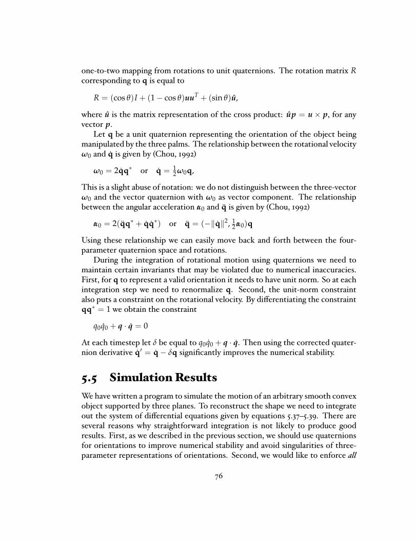
one-to-two mapping from rotations to unit quaternions. The rotation matrix Rcorresponding to q is equal to

R = (cos θ)I + (1− cos θ)uuT + (sin θ)u,

where u is the matrix representation of the cross product: up = u × p, for anyvector p.Let q be a unit quaternion representing the orientation of the object being

manipulated by the three palms. The relationship between the rotational velocityω0 and q is given by (Chou, 1992)

ω0 = 2qq∗ or q = 12 ω0q,

This is a slight abuse of notation: we do not distinguish between the three-vectorω0 and the vector quaternion with ω0 as vector component. The relationshipbetween the angular acceleration α0 and q is given by (Chou, 1992)

α0 = 2(qq∗ + qq∗) or q = (−‖q‖2, 12 α0)q

Using these relationship we can easily move back and forth between the four-parameter quaternion space and rotations.During the integration of rotational motion using quaternions we need to

maintain certain invariants that may be violated due to numerical inaccuracies.First, for q to represent a valid orientation it needs to have unit norm. So at eachintegration step we need to renormalize q. Second, the unit-norm constraintalso puts a constraint on the rotational velocity. By di�erentiating the constraintqq∗ = 1 we obtain the constraint

q0q0 + q · q = 0

At each timestep let δ be equal to q0q0 + q · q. Then using the corrected quater-nion derivative q′ = q − δq signi�cantly improves the numerical stability.

5.5 SimulationResultsWehave written a program to simulate the motion of an arbitrary smooth convexobject supported by three planes. To reconstruct the shape we need to integrateout the system of di�erential equations given by equations 5.37�5.39. There areseveral reasons why straightforward integration is not likely to produce goodresults. First, as we described in the previous section, we should use quaternionsfor orientations to improve numerical stability and avoid singularities of three-parameter representations of orientations. Second, we would like to enforce all

76

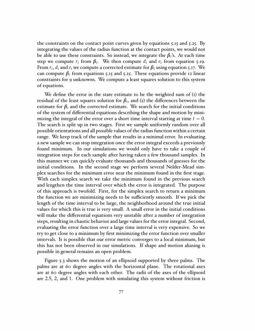
the constraints on the contact point curves given by equations 5.15 and 5.25. Byintegrating the values of the radius function at the contact points, we would notbe able to use these constraints. So instead, we integrate the βi's. At each timestep we compute ri from βi. We then compute di and ei from equation 5.19.From ri, di and ei we compute a corrected estimate for βi using equation 5.17. Wecan compute βi from equations 5.15 and 5.25. These equations provide 12 linearconstraints for 9 unknowns. We compute a least squares solution to this systemof equations.

We de�ne the error in the state estimate to be the weighted sum of (1) theresidual of the least squares solution for βi, and (2) the di�erences between theestimate for βi and the corrected estimate. We search for the initial conditionsof the system of di�erential equations describing the shape and motion by mini-mizing the integral of the error over a short time interval starting at time t = 0.The search is split up in two stages. First we sample uniformly random over allpossible orientations and all possible values of the radius function within a certainrange. We keep track of the sample that results in a minimal error. In evaluatinga new sample we can stop integration once the error integral exceeds a previouslyfound minimum. In our simulations we would only have to take a couple ofintegration steps for each sample after having taken a few thousand samples. Inthis manner we can quickly evaluate thousands and thousands of guesses for theinitial conditions. In the second stage we perform several Nelder-Mead sim-plex searches for the minimum error near the minimum found in the �rst stage.With each simplex search we take the minimum found in the previous searchand lengthen the time interval over which the error is integrated. The purposeof this approach is twofold. First, for the simplex search to return a minimumthe function we are minimizing needs to be su�ciently smooth. If we pick thelength of the time interval to be large, the neighborhood around the true initialvalues for which this is true is very small. A small error in the initial conditionswill make the di�erential equations very unstable after a number of integrationsteps, resulting in chaotic behavior and large values for the error integral. Second,evaluating the error function over a large time interval is very expensive. So wetry to get close to a minimum by �rst minimizing the error function over smallerintervals. It is possible that our error metric converges to a local minimum, butthis has not been observed in our simulations. If shape and motion aliasing ispossible in general remains an open problem.

Figure 5.3 shows the motion of an ellipsoid supported by three palms. Thepalms are at 60 degree angles with the horizontal plane. The rotational axesare at 60 degree angles with each other. The radii of the axes of the ellipsoidare 2.5, 2, and 1. One problem with simulating this system without friction is

77

Figure 5.3: An object rolling and sliding on immobile palms with gravity andcontact forces acting on it. The object is given some initial rotational velocity.The object is shown at t = 0, 0.2, . . . , 4.4 (from left to right, top to bottom). Theviewpoint is above the palms, looking down.

that if the palms are moving they continuously increase the kinetic energy of theobject. In our simulations the ellipsoid breaks contact before a signi�cant partof the object is recovered. To avoid this problem, we keep the palms in the sameposition and give the ellipsoid some initial velocity. In �gure 5.3 the object hasan initial rotational velocity of (0, 0.3, 0.3)T. In the search for initial conditionswe assume the initial rotational velocity is known. This is, of course, not veryrealistic. If we would model friction, then moving the palms would becomefeasible and we could start the system with the object at rest. In that case therotational velocitywould be zero. Our current program searches a six dimensional

78

0 0.5 1 1.5 2 2.5 3 3.5 41

1.2

1.4

1.6

1.8

2

2.2

2.4

r1

r2

r3

(a) The radius function values at thecontact points.

0 0.5 1 1.5 2 2.5 3 3.5 4

−0.5

−0.4

−0.3

−0.2

−0.1

0

0.1

0.2

(b) The four quaternion components ofthe rotational velocity.

Figure 5.4: Di�erences between real and recovered shape and motion. Realvalues are plotted as solid lines, observed values as dashed lines.

space: three dimensions for orientation and three for the values of the radiusfunction at the contact points. The reconstructed shape and motion are shownin �gure 5.4. Our program found a di�erent, but equally valid initial orientationfor the ellipsoid. Because of the symmetries of the ellipsoid, rotations of 180degrees around the principal axes result in orientations that are indistinguishable:the resulting rotational velocity and values for the radius function are identical(up to numerical error).

5.6 Shape ApproximationsGiven the recovered motion and contact curves we can also give a lower andan upper bound on the volume occupied by the entire shape. Since we assumethe object is convex, the convex hull of the contact curves in the object frameis a lower bound on the shape. Figure 5.5 shows the lower bound on the shapeobtained from the example in the previous section.We can obtain an upper bound by observing that at each contact point the

corresponding palm plane introduces a half-space constraint: the object has tolie entirely on one side of the plane. Clearly, the intersection of half-spacesalong the contact curves in the object frame forms an upper bound on theshape. Computing the intersection of half-spaces can be reduced to a convexhull problem as follows. Suppose we have a set of n points on the contact curvesand the unit normals at these points. Let pi, i = 1, . . . , n be one of the contactpoints and ni its corresponding unit normal. The half-space constraint at point i

79

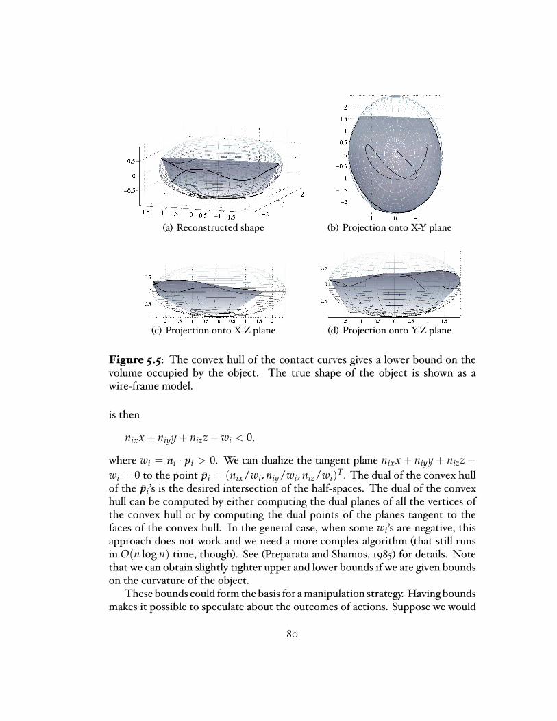
(a) Reconstructed shape (b) Projection onto X-Y plane

(c) Projection onto X-Z plane (d) Projection onto Y-Z plane

Figure 5.5: The convex hull of the contact curves gives a lower bound on thevolume occupied by the object. The true shape of the object is shown as awire-frame model.

is then

nixx + niyy + nizz − wi < 0,

where wi = ni · pi > 0. We can dualize the tangent plane nixx + niyy + nizz −wi = 0 to the point pi = (nix/wi, niy/wi, niz/wi)T. The dual of the convex hullof the pi's is the desired intersection of the half-spaces. The dual of the convexhull can be computed by either computing the dual planes of all the vertices ofthe convex hull or by computing the dual points of the planes tangent to thefaces of the convex hull. In the general case, when some wi's are negative, thisapproach does not work and we need a more complex algorithm (that still runsin O(n log n) time, though). See (Preparata and Shamos, 1985) for details. Notethat we can obtain slightly tighter upper and lower bounds if we are given boundson the curvature of the object.These bounds could form the basis for amanipulation strategy. Having bounds

makes it possible to speculate about the outcomes of actions. Suppose we would

80

Figure 5.6: Two spherical palms holding an object.

like to estimate the entire shape. One objective for a planner could be tominimizethe di�erence between the upper bound and lower bound. A simple `greedy'planner would always try to move the contact points toward points on the lowerboundwith the largest distance to the upper bound. A smarter planner would alsotake into account the path length, such that the palms would minimize nearbydi�erences between the bounds before trying to minimize faraway di�erences.This assumes we have some reasonable metric to measure distance betweenpalm/object con�gurations. This manipulation strategy is reminiscent of some ofthe work in geometric probing, but unlike probing algorithms our manipulationstrategy continuously `probes' the object. The palms cannot instantaneously movefrom one con�guration to another.Let us now consider how these bounds change if we change the shape of

the palms. We can use the shape of the palms to get tighter upper bounds onthe shape of the unknown object. Suppose we have spherical palms. Figure 5.6shows two spherical palms holding an object. Instead of taking intersections ofhalf-spaces, we can now use intersections of spheres as an upper bound. Thecontact point on palm i can be written as

ci = biRi

cos si1 cos si2sin si1 cos si2

sin si2

, (5.42)

where bi is the radius of sphere/palm i, and (si1, si2) are the spherical sensor co-ordinates. We can obtain expressions for ci by di�erentiating the right-hand sideof equation 5.42 with respect to Ri and si. The solution for the dynamics of theobject would change slightly with spherical palms, but the solution for the shapeand motion of the object would remain structurally the same. Equations 5.14

81

and 5.15 show clearly how the solution for the shape of the object depends on themotion of the contact points.If we allow some of the palms to be convex, we could actually recover con-

cavities on the object provided the radius of curvature along the concavities islarger than the radius of the palm. Allowing the object to have concavities wouldinvalidate the upper bound derived above. We can de�ne a new upper boundas the intersection of half-spaces at those points on the contact curves that arealso on the boundary of the convex hull of the curves. Assuming the palms arein�nite rays this is a true upper bound even if there exists protrusions betweendi�erent parts of the shape that have been recovered, because the protrusionscannot intersect the palms. We can also de�ne other approximate representa-tions of the shape of the object that may be closer to the true shape. Let usassume that instead of continuous contact curves we have a �nite set of pointsalong those curves. Based on this set of points we can de�ne a family of α-shapes(Edelsbrunner and Mücke, 1994). One can think of α-shapes as a generalizationof the convex hull. Suppose we compute a Delaunay triangulation of the setof points. Then informally, for a given value of α the corresponding α-shape isequal to the triangulation minus the triangles that a sphere with radius α can passthrough without intersecting any of the vertices. The entire family of α-shapesfor a set of n points can be computed in O(n2). This family oh α-shapes can beseen as a set of interpretations. Another way to represent the shape is to computea smooth interpolated surface. There are many ways to smoothly interpolate apoint set. We could use splines or iterative methods such as principal surfaces, anextension of principal curves (Hastie and Stuetzle, 1989; LeBlanc and Tibshirani,1994). Splines and principal curves can also be used in the planar case, of course.

82

C h a p t e r 6

Conclusion

6.1 ContributionsThis thesis has shown how a robot can reconstruct the local shape of an unknownsmooth convex object with strictly positive curvature along the surface. Theobject is manipulated by palms covered with tactile sensors. The object is notimmobilized by the palms, but instead moves around as the contact forces andgravity act on it. This is a novel way to combine manipulation and tactile sensingthat allows for a continuous interaction between manipulation and sensing.In chapter 3 we presented the analysis, simulation results and experimental

results for the quasistatic case. We derived expressions for the values of theradius function at the contact points and the rotational speed of the object. Thiscompletely describes the shape and motion of an unknown object as a system ofdi�erential equations. The simulation results showed that our approach workswell. We showed that �nding the initial conditions of this system of di�erentialequations corresponds to a 1D search for the center of mass: the center of masshas to lie on the vertical line through the intersection of the lines of force at thecontact points. Further research is needed on �nding these initial conditions:we can �nd a minimum of an error measure along this line, but it is not known ifthis is a global minimum.Our experimental results suggest that our approach could also work in prac-

tice. The reconstructed shape was close to the actual shape, despite signi�canterrors in the reconstructed motion of our experimental object. These errorswere caused in part by violations of the assumptions, the most important onebeing the no-friction assumption. Once we have modeled friction, we expect theperformance of our shape reconstruction method to improve considerably.It is possible that the motion of the object has discontinuities, even if the

motion of the palms is continuous. This happens when a local minimum of the

83

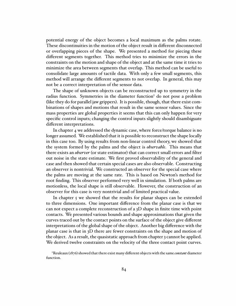
potential energy of the object becomes a local maximum as the palms rotate.These discontinuities in the motion of the object result in di�erent disconnectedor overlapping pieces of the shape. We presented a method for piecing thesedi�erent segments together. This method tries to minimize the errors in theconstraints on the motion and shape of the object and at the same time it tries tominimize the area between segments that overlap. This method can be useful toconsolidate large amounts of tactile data. With only a few small segments, thismethod will arrange the di�erent segments to not overlap. In general, this maynot be a correct interpretation of the sensor data.The shape of unknown objects can be reconstructed up to symmetry in the

radius function. Symmetries in the diameter function1 do not pose a problem(like they do for parallel jaw grippers). It is possible, though, that there exist com-binations of shapes and motions that result in the same sensor values. Since themass properties are global properties it seems that this can only happen for veryspeci�c control inputs; changing the control inputs slightly should disambiguatedi�erent interpretations.In chapter 4 we addressed the dynamic case, where force/torque balance is no

longer assumed. We established that it is possible to reconstruct the shape locallyin this case too. By using results from non-linear control theory, we showed thatthe system formed by the palms and the object is observable. This means thatthere exists an observer (or state estimator) that can correct small errors and �lterout noise in the state estimate. We �rst proved observability of the general andcase and then showed that certain special cases are also observable. Constructingan observer is nontrivial. We constructed an observer for the special case wherethe palms are moving at the same rate. This is based on Newton's method forroot �nding. This observer performed very well in simulation. If both palms aremotionless, the local shape is still observable. However, the construction of anobserver for this case is very nontrivial and of limited practical value.In chapter 5 we showed that the results for planar shapes can be extended

to three dimensions. One important di�erence from the planar case is that wecan not expect a complete reconstruction of a 3D shape in �nite time with pointcontacts. We presented various bounds and shape approximations that given thecurves traced out by the contact points on the surface of the object give di�erentinterpretations of the global shape of the object. Another big di�erence with theplanar case is that in 3D there are fewer constraints on the shape and motion ofthe object. As a result, the quasistatic approach from chapter 3 cannot be applied.We derived twelve constraints on the velocity of the three contact point curves.

1Reuleaux (1876) showed that there existmanydi�erent objectswith the same constant diameterfunction.

84

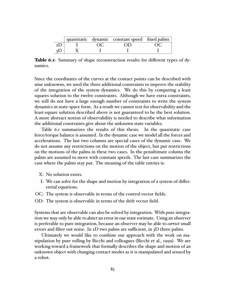
quasistatic dynamic constant speed �xed palms2D I OC OD OC3D X I I I

Table 6.1: Summary of shape reconstruction results for di�erent types of dy-namics.

Since the coordinates of the curves at the contact points can be described withnine unknowns, we used the three additional constraints to improve the stabilityof the integration of the system dynamics. We do this by computing a leastsquares solution to the twelve constraints. Although we have extra constraints,we still do not have a large enough number of constraints to write the systemdynamics in state-space form. As a result we cannot test for observability and theleast-square solution described above is not guaranteed to be the best solution.A more abstract notion of observability is needed to describe what informationthe additional constraints give about the unknown state variables.Table 6.1 summarizes the results of this thesis. In the quasistatic case

force/torque balance is assumed. In the dynamic case we model all the forces andaccelerations. The last two columns are special cases of the dynamic case. Wedo not assume any restrictions on the motion of the object, but put restrictionson the motions of the palms in these two cases. In the penultimate column thepalms are assumed to move with constant speeds. The last case summarizes thecase where the palms stay put. The meaning of the table entries is:

X: No solution exists.I: We can solve for the shape and motion by integration of a system of di�er-ential equations.

OC: The system is observable in terms of the control vector �elds.OD: The system is observable in terms of the drift vector �eld.

Systems that are observable can also be solved by integration. With pure integra-tion wemay only be able to detect an error in our state estimate. Using an observeris preferable to pure integration, because an observer may be able to correct smallerrors and �lter out noise. In 2D two palms are su�cient, in 3D three palms.Ultimately we would like to combine our approach with the work on ma-

nipulation by pure rolling by Bicchi and colleagues (Bicchi et al., 1999). We areworking toward a framework that formally describes the shape and motion of anunknown object with changing contact modes as it is manipulated and sensed bya robot.

85

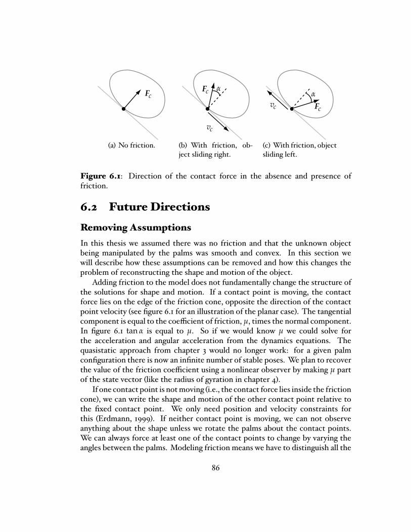
Fc

(a) No friction.

α

vc

Fc

(b) With friction, ob-ject sliding right.

Fc

α

vc

(c) With friction, objectsliding left.

Figure 6.1: Direction of the contact force in the absence and presence offriction.

6.2 FutureDirectionsRemoving AssumptionsIn this thesis we assumed there was no friction and that the unknown objectbeing manipulated by the palms was smooth and convex. In this section wewill describe how these assumptions can be removed and how this changes theproblem of reconstructing the shape and motion of the object.Adding friction to the model does not fundamentally change the structure of

the solutions for shape and motion. If a contact point is moving, the contactforce lies on the edge of the friction cone, opposite the direction of the contactpoint velocity (see �gure 6.1 for an illustration of the planar case). The tangentialcomponent is equal to the coe�cient of friction, µ, times the normal component.In �gure 6.1 tan α is equal to µ. So if we would know µ we could solve forthe acceleration and angular acceleration from the dynamics equations. Thequasistatic approach from chapter 3 would no longer work: for a given palmcon�guration there is now an in�nite number of stable poses. We plan to recoverthe value of the friction coe�cient using a nonlinear observer by making µ partof the state vector (like the radius of gyration in chapter 4).If one contact point is notmoving (i.e., the contact force lies inside the friction

cone), we can write the shape and motion of the other contact point relative tothe �xed contact point. We only need position and velocity constraints forthis (Erdmann, 1999). If neither contact point is moving, we can not observeanything about the shape unless we rotate the palms about the contact points.We can always force at least one of the contact points to change by varying theangles between the palms. Modeling friction means we have to distinguish all the

86

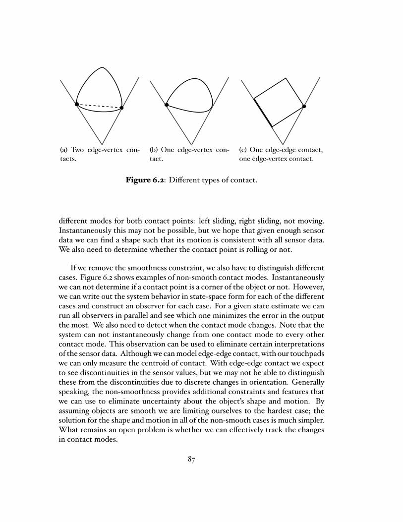
(a) Two edge-vertex con-tacts.

(b) One edge-vertex con-tact.

(c) One edge-edge contact,one edge-vertex contact.

Figure 6.2: Di�erent types of contact.

di�erent modes for both contact points: left sliding, right sliding, not moving.Instantaneously this may not be possible, but we hope that given enough sensordata we can �nd a shape such that its motion is consistent with all sensor data.We also need to determine whether the contact point is rolling or not.

If we remove the smoothness constraint, we also have to distinguish di�erentcases. Figure 6.2 shows examples of non-smooth contact modes. Instantaneouslywe can not determine if a contact point is a corner of the object or not. However,we can write out the system behavior in state-space form for each of the di�erentcases and construct an observer for each case. For a given state estimate we canrun all observers in parallel and see which one minimizes the error in the outputthe most. We also need to detect when the contact mode changes. Note that thesystem can not instantaneously change from one contact mode to every othercontact mode. This observation can be used to eliminate certain interpretationsof the sensor data. Althoughwe canmodel edge-edge contact, with our touchpadswe can only measure the centroid of contact. With edge-edge contact we expectto see discontinuities in the sensor values, but we may not be able to distinguishthese from the discontinuities due to discrete changes in orientation. Generallyspeaking, the non-smoothness provides additional constraints and features thatwe can use to eliminate uncertainty about the object's shape and motion. Byassuming objects are smooth we are limiting ourselves to the hardest case; thesolution for the shape and motion in all of the non-smooth cases is much simpler.What remains an open problem is whether we can e�ectively track the changesin contact modes.

87

Di�erent Representations of ShapeThe contact kinematics lead naturally to a description of the shape of an object interms of the curvature at the contact points. One disadvantage of this approach isthat the shape has an in�nite number of degrees of freedom. Although this allowsus to reconstruct any smooth convex shape, in many cases it may be su�cient tohave a reasonable approximation. We could, for instance, pick n control pointsthat are radially equally spaced. A closed spline interpolation through those npoints is then one possible shape approximation. So now the shape has only ndegrees of freedom. If we want to do something fancier, we could use Fourierand wavelet transforms. There has been a large amount of research in computervision and pattern matching on representing shapes. With future research wewould like to explore how results in those areas can be used for tactile shapereconstruction. In section 4.7 we mentioned alpha shapes and principal curves asapproximate shape representations. We would also like to �nd ways to use thesedi�erent representations to guide the manipulation.

Di�erentObserversObserver design for nonlinear systems is still an active area of research. Theobserver described in chapter 4 is relatively simple. It is easy to implement, butis computationally very expensive. In future research we would like to developobservers that do not rely as heavily on numerical methods. Many observersuse the following approach. For a given state q we can de�ne a transformZ : q → z, such that the transformed system is in some canonical form. Oftenthe transformed system looks like

z = Az + f (z, u) (6.1)y = Cz. (6.2)

That is, the system is almost linear, except for some nonlinearities that dependon the controls. To guarantee exponential convergence certain constraints on fneed to be satis�ed. Inmany cases the control inputs can be ignored, if we assumethe control inputs are piecewise constant. Typically, the coordinate transform isvalid only locally and needs to be recomputed at each time step. An example ofthis type of observer can be found in e.g. (Gauthier et al., 1992). Gauthier et al.assumed a single-output system without inputs, but Bornard and Hammouri(1991) showed that this observer can be generalized to multi-input-multi-outputsystems. If we assume the sensor values are reliable, we can construct a so-called reduced-order observer, which, as the name suggests, only tries to observethose state variables which are not part of the output (Besançon and Hammouri,

88

1995). The observers mentioned above all use a Lie-algebraic approach. Othercommon techniques include: Lyapunov methods (Thau, 1973; Kou et al., 1975),and linearization by nonlinear output injection (Krener and Isidori, 1983; Bestleand Zeitz, 1983). We would like to explore how these techniques can be appliedto the tactile shape reconstruction problem.

Tactile slamSimultaneous localization andmapping (slam) is an important problem inmobilerobotics. The slam problem can be stated as: how can a mobile robot e�cientlybuild a map of an unknown environment and at the same time keep track ofwhere it is on the map? A common failure mode is that a robot returns to a placewhere it has been before, but classi�es it as new place on the map. With thetactile shape reconstruction method proposed in this thesis we run into a similarproblem. If the sensors cover the same part of the surface many times, thereis no constraint that forces the contact point curves to lie on the same surface.So we need a strategy to consolidate all data into one surface (or a probabilitydistribution of surfaces, if one prefers a probabilistic approach). Note that thepresence of non-smooth features on the surface will make the tactile localizationproblem signi�cantly easier (Okamura and Cutkosky, 2001). In section 3.7 weproposed a method to consolidate con�icting data by averaging, but we wouldlike to do better. We expect that some results for the slam problem will transferto tactile shape reconstruction.In computer vision and pattern matching the localization problem is often

called the registration (or correspondence) problem. From this area we may beable to borrow techniques to compare di�erent shapes. For instance, we coulduse distance metrics that are invariant with respect to rotation, scale, or both(Arkin et al., 1991; Huttenlocher and Kedem, 1990).

Other Sensing StrategiesBesides the model of planar palms, there are many other ways to reconstruct theshape of an unknown moving object with tactile sensors. One extension is tochange the shape of the palms. In the previous chapters we described how themodel can be extended to circular and spherical palms. An advantage of concavepalms is that with less manipulation we can cover more of the shape, since agrasp with these palms comes closer to an enveloping grasp. Further researchis needed to quantify this claim. The minimum radius of curvature along thepalms should be chosen such that there is always just one contact point on eachpalm. However, if the palms can detect multiple contacts, it makes more sense

89

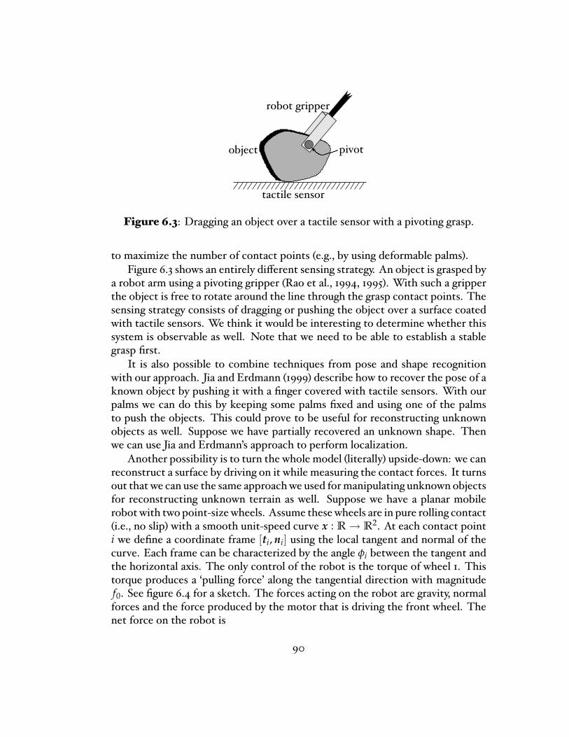
object

robot gripper

pivot

tactile sensor

Figure 6.3: Dragging an object over a tactile sensor with a pivoting grasp.

to maximize the number of contact points (e.g., by using deformable palms).Figure 6.3 shows an entirely di�erent sensing strategy. An object is grasped by

a robot arm using a pivoting gripper (Rao et al., 1994, 1995). With such a gripperthe object is free to rotate around the line through the grasp contact points. Thesensing strategy consists of dragging or pushing the object over a surface coatedwith tactile sensors. We think it would be interesting to determine whether thissystem is observable as well. Note that we need to be able to establish a stablegrasp �rst.It is also possible to combine techniques from pose and shape recognition

with our approach. Jia and Erdmann (1999) describe how to recover the pose of aknown object by pushing it with a �nger covered with tactile sensors. With ourpalms we can do this by keeping some palms �xed and using one of the palmsto push the objects. This could prove to be useful for reconstructing unknownobjects as well. Suppose we have partially recovered an unknown shape. Thenwe can use Jia and Erdmann's approach to perform localization.Another possibility is to turn the whole model (literally) upside-down: we can

reconstruct a surface by driving on it while measuring the contact forces. It turnsout that we can use the same approachwe used formanipulating unknown objectsfor reconstructing unknown terrain as well. Suppose we have a planar mobilerobot with two point-size wheels. Assume these wheels are in pure rolling contact(i.e., no slip) with a smooth unit-speed curve x : R → R2. At each contact pointi we de�ne a coordinate frame [ti, ni] using the local tangent and normal of thecurve. Each frame can be characterized by the angle φi between the tangent andthe horizontal axis. The only control of the robot is the torque of wheel 1. Thistorque produces a `pulling force' along the tangential direction with magnitudef0. See �gure 6.4 for a sketch. The forces acting on the robot are gravity, normalforces and the force produced by the motor that is driving the front wheel. Thenet force on the robot is

90

n1t1

n2 t2

d1 d2

x(s)

cm

gravity

Figure6.4: Amobile robot consisting of twomass-less rods d1 and d2 connectedat the center of mass cm in contact with a curve. The wheels are at the end pointsof d1 and d2.

F = f0t1 + f1n1 + f2n2 + Fg = ma, (6.3)

where f0 is the magnitude of the force produced by the motor, f1 and f2 are themagnitudes of the normal forces and Fg is the gravitational force. The net torqueon the robot is

τ = f0d1 × t1 + f1d1 × n1 + f2d2 × n2

= − f0d1 · n1 + f1d1 · t1 + f2d2 · t2 = mρ2α, (6.4)

where di, i = 1, 2, is the vector from the center of mass to wheel i. For simplicity,assume d1 and d2 are of equal length and make a right angle with each other.We assume that the wheels always stay in contact with the curve. This

imposes constraints on (derivatives of ) the position of the robot. Let cm denotethe position of the center of mass, xi the point on the curve in contact with wheeli, and vi the velocity of contact point i. The position constraints for wheel i canbe written as

cm + di = xi (6.5)v + ω × di = viti (6.6)a + α × di + ω × (ω × di) = viti + κiv2

i ni (6.7)

The right-hand side of the last constraint follows from the Frenet formulas.We will assume that the control input f0 is chosen such that the velocity atwheel 1 is constant. Let us the de�ne the state q of the system as the vector(φ0, ω, x1, x2, v2)T. The behavior of the system can then be described by the

91

following system of di�erential equations

φ0 = ω (6.8)ω = α (6.9)x1 = v1t1 (6.10)x2 = v2t2 (6.11)v2 = (a + α × d2 − ω2d2) · t2 (6.12)

Note that since we drive wheel 1 at a constant speed, v1 is equal to zero andwe do not need to make v1 part of the state. It can be shown that if we canmeasure the magnitude of the one of the contact forces, we can solve for theacceleration and angular acceleration from the dynamics described above. Wecan measure the contact force with strain gauges. The above system is not instate-space form, since we do not have an expression for the rate of change inthe contact force as a function of the state variables. Further research is neededto either reformulate this problem or construct another kind of state estimatorwith observer-like properties.

92

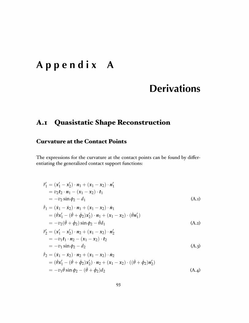
A p p e n d i x A

Derivations

A.1 Quasistatic ShapeReconstruction

Curvature at the Contact Points

The expressions for the curvature at the contact points can be found by di�er-entiating the generalized contact support functions:

r′1 = (x′1 − x′2) · n1 + (x1 − x2) · n′1= v2t2 · n1 − (x1 − x2) · t1

= −v2 sin φ2 − d1 (A.1)˙r1 = (x1 − x2) · n1 + (x1 − x2) · n1

= (θx′1 − (θ + φ2)x′2) · n1 + (x1 − x2) · (θn′1)

= −v2(θ + φ2) sin φ2 − θd1 (A.2)

r′2 = (x′1 − x′2) · n2 + (x1 − x2) · n′2= −v1t1 · n2 − (x1 − x2) · t2

= −v1 sin φ2 − d2 (A.3)˙r2 = (x1 − x2) · n2 + (x1 − x2) · n2

= (θx′1 − (θ + φ2)x′2) · n2 + (x1 − x2) · ((θ + φ2)n′2)

= −v1θ sin φ2 − (θ + φ2)d2 (A.4)

93

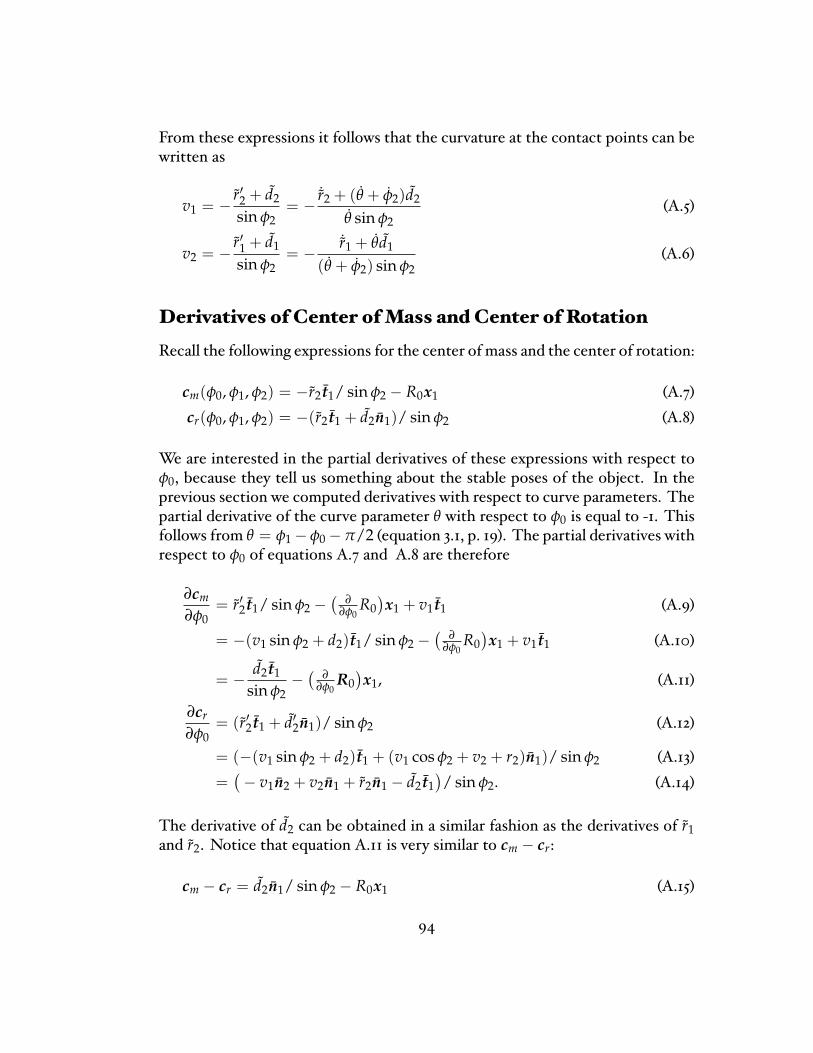
From these expressions it follows that the curvature at the contact points can bewritten as

v1 = −r′2 + d2

sin φ2= −

˙r2 + (θ + φ2)d2

θ sin φ2(A.5)

v2 = −r′1 + d1

sin φ2= −

˙r1 + θd1

(θ + φ2) sin φ2(A.6)

Derivatives of Center ofMass andCenter of RotationRecall the following expressions for the center of mass and the center of rotation:

cm(φ0, φ1, φ2) = −r2t1/ sin φ2 − R0x1 (A.7)cr(φ0, φ1, φ2) = −(r2t1 + d2n1)/ sin φ2 (A.8)

We are interested in the partial derivatives of these expressions with respect toφ0, because they tell us something about the stable poses of the object. In theprevious section we computed derivatives with respect to curve parameters. Thepartial derivative of the curve parameter θ with respect to φ0 is equal to -1. Thisfollows from θ = φ1 − φ0 −π/2 (equation 3.1, p. 19). The partial derivatives withrespect to φ0 of equations A.7 and A.8 are therefore

∂cm

∂φ0= r′2t1/ sin φ2 −

(∂

∂φ0R0)x1 + v1t1 (A.9)

= −(v1 sin φ2 + d2)t1/ sin φ2 −(

∂∂φ0

R0)x1 + v1t1 (A.10)

= − d2t1

sin φ2−(

∂∂φ0

R0)x1, (A.11)

∂cr

∂φ0= (r′2t1 + d′2n1)/ sin φ2 (A.12)

= (−(v1 sin φ2 + d2)t1 + (v1 cos φ2 + v2 + r2)n1)/ sin φ2 (A.13)=(− v1n2 + v2n1 + r2n1 − d2t1

)/ sin φ2. (A.14)

The derivative of d2 can be obtained in a similar fashion as the derivatives of r1and r2. Notice that equation A.11 is very similar to cm − cr:

cm − cr = d2n1/ sin φ2 − R0x1 (A.15)

94

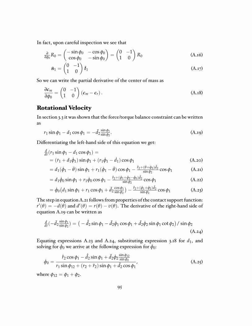
In fact, upon careful inspection we see that

∂∂φ0

R0 =(− sin φ0 − cos φ0cos φ0 − sin φ0

)=(

0 −11 0

)R0 (A.16)

n1 =(

0 −11 0

)t1 (A.17)

So we can write the partial derivative of the center of mass as

∂cm

∂φ0=(

0 −11 0

)(cm − cr) . (A.18)

Rotational VelocityIn section 3.3 it was shown that the force/torque balance constraint can be writtenas

r1 sin φ1 − d1 cos φ1 = −d2sin φ1sin φ2

. (A.19)

Di�erentiating the left-hand side of this equation we get:ddt (r1 sin φ1 − d1 cos φ1) =

= (r1 + d1φ1) sin φ1 + (r1φ1 − d1) cos φ1 (A.20)

= d1(φ1 − θ) sin φ1 + r1(φ1 − θ) cos φ1 −˙r2+(θ+φ2)d2

sin φ2cos φ1 (A.21)

= d1φ0 sin φ1 + r1φ0 cos φ1 −˙r2+(φ1+φ2−φ0)d2

sin φ2cos φ1 (A.22)

= φ0(d1 sin φ1 + r1 cos φ1 + d2

cos φ1sin φ2

)− ˙r2+(φ1+φ2)d2

sin φ2cos φ1 (A.23)

The step in equationA.21 follows fromproperties of the contact support function:r′(θ) = −d(θ) and d′(θ) = r(θ)− v(θ). The derivative of the right-hand side ofequation A.19 can be written as

ddt (−d2

sin φ1sin φ2

) =(− ˙d2 sin φ1 − d2φ1 cos φ1 + d2φ2 sin φ1 cot φ2

)/ sin φ2

(A.24)

Equating expressions A.23 and A.24, substituting expression 3.18 for d1, andsolving for φ0 we arrive at the following expression for φ0:

φ0 =˙r2 cos φ1 − ˙d2 sin φ1 + d2φ2

sin φ12sin φ2

r1 sin φ12 + (r2 + r2) sin φ1 + d2 cos φ1, (A.25)

where φ12 = φ1 + φ2.

95

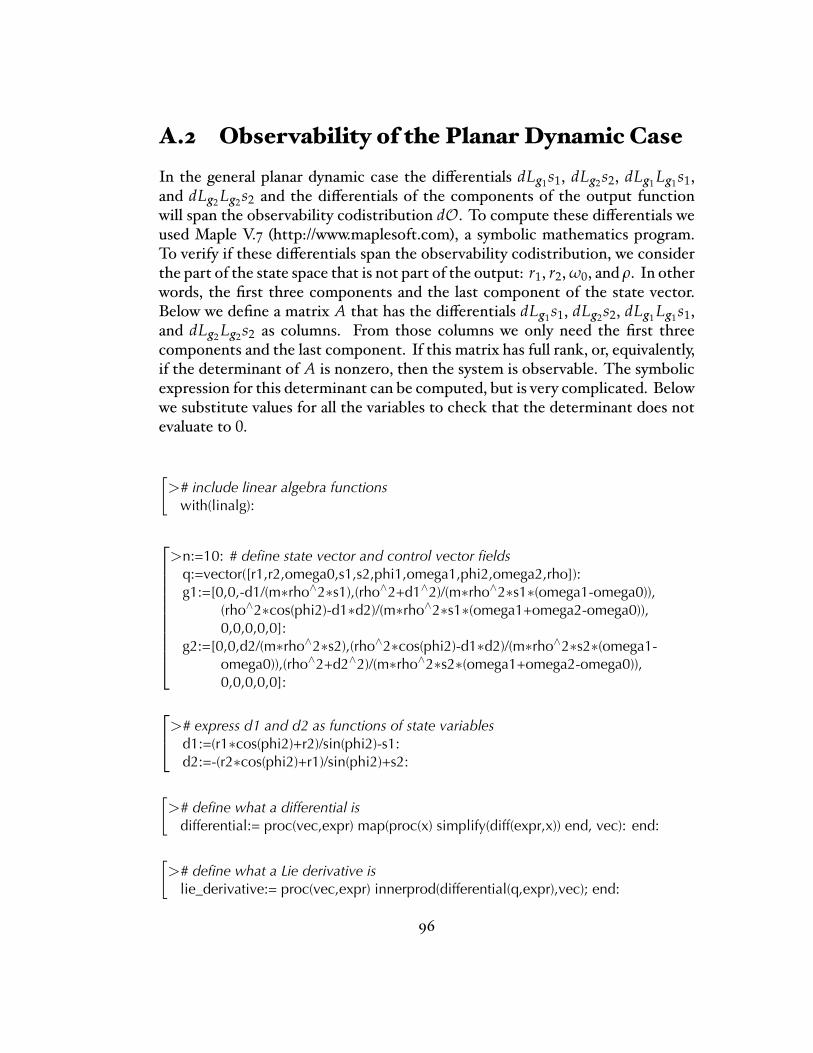
A.2 Observability of the PlanarDynamic CaseIn the general planar dynamic case the di�erentials dLg1s1, dLg2s2, dLg1 Lg1s1,and dLg2 Lg2s2 and the di�erentials of the components of the output functionwill span the observability codistribution dO. To compute these di�erentials weused Maple V.7 (http://www.maplesoft.com), a symbolic mathematics program.To verify if these di�erentials span the observability codistribution, we considerthe part of the state space that is not part of the output: r1, r2,ω0, and ρ. In otherwords, the �rst three components and the last component of the state vector.Below we de�ne a matrix A that has the di�erentials dLg1s1, dLg2s2, dLg1 Lg1s1,and dLg2 Lg2s2 as columns. From those columns we only need the �rst threecomponents and the last component. If this matrix has full rank, or, equivalently,if the determinant of A is nonzero, then the system is observable. The symbolicexpression for this determinant can be computed, but is very complicated. Belowwe substitute values for all the variables to check that the determinant does notevaluate to 0.

[># include linear algebra functionswith(linalg):

>n:=10: # de�ne state vector and control vector �eldsq:=vector([r1,r2,omega0,s1,s2,phi1,omega1,phi2,omega2,rho]):g1:=[0,0,-d1/(m∗rho∧2∗s1),(rho∧2+d1∧2)/(m∗rho∧2∗s1∗(omega1-omega0)),

(rho∧2∗cos(phi2)-d1∗d2)/(m∗rho∧2∗s1∗(omega1+omega2-omega0)),0,0,0,0,0]:

g2:=[0,0,d2/(m∗rho∧2∗s2),(rho∧2∗cos(phi2)-d1∗d2)/(m∗rho∧2∗s2∗(omega1-omega0)),(rho∧2+d2∧2)/(m∗rho∧2∗s2∗(omega1+omega2-omega0)),0,0,0,0,0]:># express d1 and d2 as functions of state variables

d1:=(r1∗cos(phi2)+r2)/sin(phi2)-s1:d2:=-(r2∗cos(phi2)+r1)/sin(phi2)+s2:

[># de�ne what a differential isdifferential:= proc(vec,expr) map(proc(x) simplify(diff(expr,x)) end, vec): end:

[># de�ne what a Lie derivative islie_derivative:= proc(vec,expr) innerprod(differential(q,expr),vec); end:

96

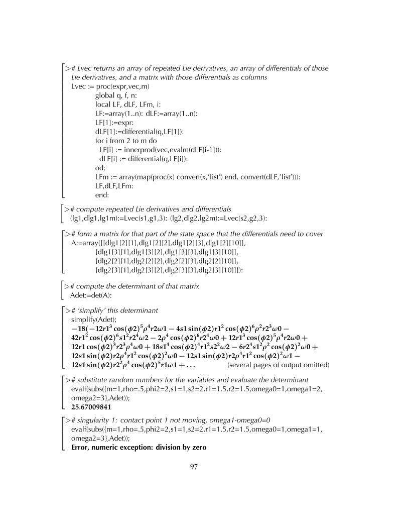
># Lvec returns an array of repeated Lie derivatives, an array of differentials of thoseLie derivatives, and a matrix with those differentials as columnsLvec := proc(expr,vec,m)

global q, f, n:local LF, dLF, LFm, i:LF:=array(1..n): dLF:=array(1..n):LF[1]:=expr:dLF[1]:=differential(q,LF[1]):for i from 2 to m doLF[i] := innerprod(vec,evalm(dLF[i-1])):dLF[i] := differential(q,LF[i]):

od;LFm := array(map(proc(x) convert(x,'list') end, convert(dLF,'list'))):LF,dLF,LFm:end:[

># compute repeated Lie derivatives and differentials(lg1,dlg1,lg1m):=Lvec(s1,g1,3): (lg2,dlg2,lg2m):=Lvec(s2,g2,3):

># form a matrix for that part of the state space that the differentials need to coverA:=array([[dlg1[2][1],dlg1[2][2],dlg1[2][3],dlg1[2][10]],

[dlg1[3][1],dlg1[3][2],dlg1[3][3],dlg1[3][10]],[dlg2[2][1],dlg2[2][2],dlg2[2][3],dlg2[2][10]],[dlg2[3][1],dlg2[3][2],dlg2[3][3],dlg2[3][10]]]):[

># compute the determinant of that matrixAdet:=det(A):

># `simplify' this determinantsimplify(Adet);−18(−12r13 cos(φ2)5ρ4r2ω1 − 4s1 sin(φ2)r12 cos(φ2)6ρ2r23ω0 −42r12 cos(φ2)6s12r24ω2 − 2ρ4 cos(φ2)6r24ω0 + 12r13 cos(φ2)5ρ4r2ω0 +12r1 cos(φ2)3r23ρ4ω0 + 18s14 cos(φ2)4r12s22ω2 − 6r24s12ρ2 cos(φ2)2ω0 +12s1 sin(φ2)r2ρ4r12 cos(φ2)2ω0 − 12s1 sin(φ2)r2ρ4r12 cos(φ2)2ω1 −12s1 sin(φ2)r22ρ4 cos(φ2)5r1ω1 + . . . (several pages of output omitted)># substitute random numbers for the variables and evaluate the determinantevalf(subs({m=1,rho=.5,phi2=2,s1=1,s2=2,r1=1.5,r2=1.5,omega0=1,omega1=2,omega2=3},Adet));25.67009841># singularity 1: contact point 1 not moving, omega1-omega0=0evalf(subs({m=1,rho=.5,phi2=2,s1=1,s2=2,r1=1.5,r2=1.5,omega0=1,omega1=1,omega2=3},Adet));Error, numeric exception: division by zero

97

># singularity 2: contact point 2 not moving, omega1+omega2-omega0=0evalf(subs({m=1,rho=.5,phi2=2,s1=1,s2=2,r1=1.5,r2=1.5,omega0=2,omega1=1,omega2=1},Adet));Error, numeric exception: division by zero># palms move at same rate, omega2=0evalf(subs({m=1,rho=.5,phi2=2,s1=1,s2=2,r1=1.5,r2=1.5,omega0=1,omega1=2,omega2=0},Adet));1647.940473># palm 1 is not moving, omega1=0evalf(subs({m=1,rho=.5,phi2=2,s1=1,s2=2,r1=1.5,r2=1.5,omega0=1,omega1=0,omega2=2},Adet));1634.446156

A.3 Force/TorqueBalance inThreeDimensionsIn two dimensions, force/torque balance of an object resting on two palms can beinterpreted in the following geometric way: the object is in force/torque balanceif and only if the lines through the normals at the contact points intersect thevertical line through the center of mass at one common point. In other words, wecan �nd the X-coordinate of the center of mass if we know the contact points andthe contact normals. For a three-dimensional object resting on three palms onecan derive a similar constraint. The derivation of the geometric interpretationin two dimensions is analogous to the three-dimensional case.Let ni be the normal at contact point ci, i = 1, 2, 3 and let fi be the magnitude

of the normal force at contact point ci. Finally, let cm be the position of thecenter of mass. Without loss of generality we assume that the magnitude of thegravitational force is 1. We can then write the force/torque balance constraint as:

Force balance: ∑ fini = nz (A.26)

Torque balance: ∑ fi(ci − cm)× ni =( 0

00

)(A.27)

Here, nz =( 0

01

)is the normal parallel to the Z-axis. We also require that all fi's

are greater than or equal to 0. The solution for equation A.26 is

f1 =(n2 × n3) · nz

(n1 × n2) · n3, f2 =

(n3 × n1) · nz

(n1 × n2) · n3, f3 =

(n1 × n2) · nz

(n1 × n2) · n3

98

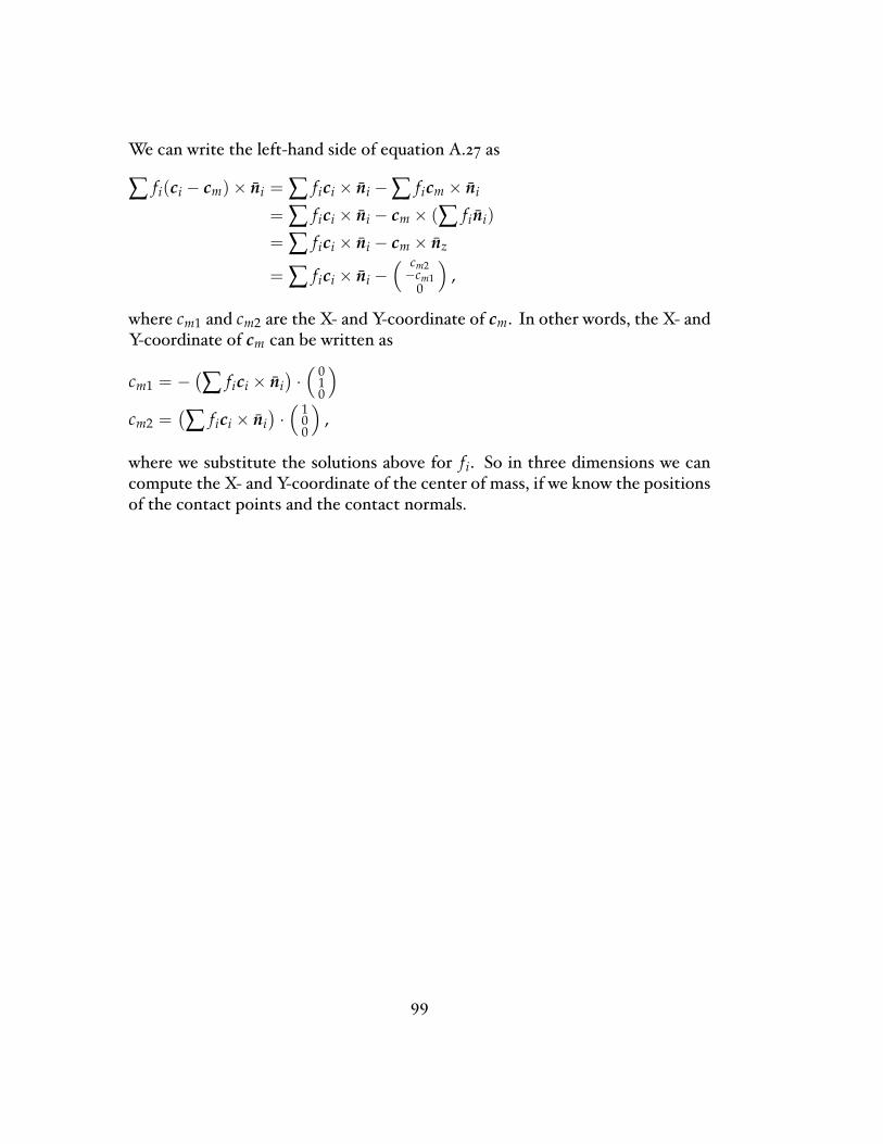
We can write the left-hand side of equation A.27 as

∑ fi(ci − cm)× ni = ∑ fici × ni −∑ ficm × ni

= ∑ fici × ni − cm × (∑ fini)

= ∑ fici × ni − cm × nz

= ∑ fici × ni −( cm2−cm1

0

),

where cm1 and cm2 are the X- and Y-coordinate of cm. In other words, the X- andY-coordinate of cm can be written as

cm1 = −(∑ fici × ni

)·( 0

10

)cm2 =

(∑ fici × ni

)·( 1

00

),

where we substitute the solutions above for fi. So in three dimensions we cancompute the X- and Y-coordinate of the center of mass, if we know the positionsof the contact points and the contact normals.

99

R e f e r e n c e s

Abell, T. and Erdmann, M. A. (1995). Stably supported rotations of a planarpolygon with two frictionless contacts. In Proceedings of the 1995 IEEE/RSJ In-ternational Conference on Intelligent Robots and Systems, pages 411�418, Pittsburgh,Pennsylvania.

Akella, S., Huang, W. H., Lynch, K. M., and Mason, M. T. (2000). Parts feedingon a conveyor with a one joint robot. Algorithmica, 26:313�344.

Akella, S. and Mason, M. T. (1999). Using partial sensor information to orientparts. International Journal of Robotics Research, 18(10):963�997.

Allen, P. K. (1988). Integrating vision and touch for object recognition tasks.International Journal of Robotics Research, 7(6):15�33.

Allen, P. K. and Michelman, P. (1990). Acquisition and interpretation of 3-Dsensor data from touch. IEEE Transactions on Robotics and Automation, 6(4):397�404.

Allen, P. K. and Roberts, K. S. (1989). Haptic object recognition using a multi-�ngered dextrous hand. In Proceedings of the 1989 IEEE International Conferenceon Robotics and Automation, pages 342�347, Scottsdale, AZ.

Ando, S. and Shinoda, H. (1995). Ultrasonic emission tactile sensing. IEEEControlSystems, 15(1):61�69.

Arkin, E., Held, M., Mitchell, J., and Skiena, S. (1998). Recognizing polygonalparts from width measurements. Computational Geometry: Theory and Applica-tions, 9(4):237�246.

Arkin, E. M., Chew, L. P., Huttenlocher, D. P., Kedem, K., and Mitchell, J. S. B.(1991). An e�ciently computablemetric for comparing polygonal shapes. IEEETransactions on Pattern Analysis andMachine Intelligence, 13(3):209�216.

Berretty, R.-P. (2000). Geometric Design of Part Feeders. PhD thesis, UtrechtUniversity.

101

Berretty, R.-P., Goldberg, K., Overmars, M.H., and Van der Stappen, A. F. (1998).Computing fence designs for orienting parts. Computational Geometry: Theoryand Applications, 10:249�262.

Besançon, G. and Hammouri, H. (1995). Reduced order observer for a classof non-uniformly observable systems. In Proceedings of the 34th Conference onDecision & Control, pages 121�125, New Orleans, LA.

Bestle, D. and Zeitz, M. (1983). Canonical form observer design for nonlineartime-variable systems. International Journal of Control, 38(2):419�431.

Bicchi, A., Marigo, A., and Prattichizzo, D. (1999). Dexterity through rolling:Manipulation of unknown objects. In Proceedings of the 1999 IEEE InternationalConference on Robotics and Automation, pages 1583�1588, Detroit, Michigan.

Böhringer, K. F., Bhatt, V., Donald, B. R., and Goldberg, K. Y. (2000a). Al-gorithms for sensorless manipulation using a vibrating surface. Algorithmica,26(3/4):389�429.

Böhringer, K.-F., Donald, B. R., Kavraki, L. E., and Lamiraux, F. (2000b). Partorientation with one or two stable equilibria using programmable force �elds.IEEE Transactions on Robotics and Automation, 16(2):157�170.

Böhringer, K. F., Donald, B. R., and MacDonald, N. C. (1996). Upper andlower bounds for programmable vector �elds with applications to MEMS andvibratory plate parts feeders. In Overmars, M. and Laumond, J.-P., editors,Workshop on the Algorithmic Foundations of Robotics, pages 255�276. A. K. Peters.

Böhringer, K. F., Donald, B. R., and MacDonald, N. C. (1999). Programmablevector �elds for distributedmanipulation, with applications toMEMS actuatorarrays and vibratory parts feeders. International Journal of Robotics Research,18(2):168�200.

Boissonnat, J. D. and Yvinec, M. (1992). Probing a scene of nonconvex polyhedra.Algorithmica, 8:321�342.

Bornard, G. and Hammouri, H. (1991). A high gain observer for a class ofuniformly observable systems. In Proceedings of the 30th Conference on Decision &Control, pages 1494�1496, Brighton, England.

Cai, C. S. and Roth, B. (1986). On the planar motion of rigid bodies with pointcontact. Mechanism andMachine Theory, 21(6):453�466.

102

Cai, C. S. and Roth, B. (1987). On the spatial motion of a rigid body with pointcontact. In Proceedings of the 1987 IEEE International Conference on Robotics andAutomation, pages 686�695.

Charlebois, M., Gupta, K., and Payandeh, S. (1996). Curvature based shapeestimation using tactile sensing. In Proceedings of the 1996 IEEE InternationalConference on Robotics and Automation, pages 3502�3507.

Charlebois, M., Gupta, K., and Payandeh, S. (1997). Shape description of gen-eral, curved surfaces using tactile sensing and surface normal information. InProceedings of the 1997 IEEE International Conference on Robotics and Automation,pages 2819�2824.

Chen, N., Rink, R., and Zhang, H. (1996). Local object shape from tactile sensing.In Proceedings of the 1996 IEEEInternationalConference onRobotics andAutomation,pages 3496�3501.

Chen, Y.-B. and Ierardi, D. (1995). The complexity of oblivious plans for orientingand distinguishing polygonal parts. Algorithmica, 14.

Choi, K. K., Jiang, S. L., and Li, Z. (1998). Multi�ngered robotic hands: Contactexperiments using tactile sensors. In Proceedings of the 1998 IEEE InternationalConference on Robotics and Automation, pages 2268�2273, Leuven, Belgium.

Chou, J. C. (1992). Quaternion kinematic and dynamic di�erential equations.IEEE Transactions on Robotics and Automation, 8(1):53�64.

Coelho Jr., J. A. and Grupen, R. A. (1996). Online grasp synthesis. In Proceedingsof the 1996 IEEEInternationalConference onRobotics andAutomation, Minneapolis,MN.

Cole, R. and Yap, C. K. (1987). Shape from probing. Journal of Algorithms,8(1):19�38.

Cutkosky,M.R. (1985). RoboticGraspingandFineManipulation. Kluwer, Dordrecht;Boston.

Cutkosky,M.R. andHyde, J.M. (1993). Manipulation controlwith dynamic tactilesensing. InProc. SixthInternationalSymposiumonRoboticsResearch, HiddenValley,Pennsylvania.

Dobkin, D., Edelsbrunner, H., and Yap, C. K. (1986). Probing convex polytopes.In Proceedings of the Eighteenth Annual ACM Symposium on Theory of Computing,pages 424�432, Berkeley, California.

103

Edelsbrunner, H. andMücke, E. P. (1994). Three-dimensional alpha shapes. ACMTransactions on Graphics (TOG), 13(1):43�72.

Ellis, R. E. (1992). Planning tactile recognition in two and three dimensions.International Journal of Robotics Research, 11(2):87�111.

Eppstein, D. (1990). Reset sequences for monotonic automata. SIAMJ. Comput-ing, 19(3):500�510.

Erdmann, M. A. (1995). Understanding action and sensing by designing action-based sensors. International Journal of Robotics Research, 14(5):483�509.

Erdmann,M. A. (1998). An exploration of nonprehensile two-palmmanipulation:Planning and execution. International Journal of Robotics Research, 17(5).

Erdmann, M. A. (1999). Shape recovery from passive locally dense tactile data.In Agarwal, P. K., Kavraki, L. E., and Mason, M. T., editors, Robotics: TheAlgorithmic Perspective. A.K. Peters.

Erdmann, M. A. and Mason, M. T. (1988). An exploration of sensorless manipu-lation. IEEE Journal of Robotics and Automation, 4(4):369�379.

Erdmann, M. A., Mason, M. T., and Van¥£ek, Jr., G. (1993). Mechanical partsorienting: The case of a polyhedron on a table. Algorithmica, 10:226�247.

Fearing, R. S. (1984). Simpli�ed grasping and manipulation with dextrous robothands. In Proceedings of the 1984 American Control Conference, pages 32�38, SanDiego, California.

Fearing, R. S. (1990). Tactile sensing for shape interpretation. In Venkataraman,S. T. and Iberall, T., editors, Dexterous Robot Hands, chapter 10, pages 209�238.Springer Verlag, Berlin; Heidelberg; New York.

Fearing, R. S. and Binford, T. O. (1988). Using a cylindrical tactile sensor fordetermining curvature. In Proceedings of the 1988 IEEE International Conferenceon Robotics and Automation, pages 765�771.

Gaston, P. C. and Lozano-Pérez, T. (1984). Tactile recognition and localizationusing object models: The case of polyhedra on a plane. IEEE Transactions onPattern Analysis andMachine Intelligence, 6(3):257�266.

Gauthier, J. P., Hammouri, H., and Othman, S. (1992). A simple observer fornonlinear systems applications to bioreactors. IEEE Transactions on AutomaticControl, 37(6):875�880.

104

Goldberg, K. Y. (1993). Orienting polygonal parts without sensors. Algorithmica,10(3):201�225.

Goldberg, K. Y. and Bajcsy, R. (1984). Active touch and robot perception. Cogni-tion and Brain Theory, 7(2):199�214.

Golub, G. H. and Loan, C. F. V. (1996). Matrix Computations. Johns HopkinsUniversity Press, third edition.

Grimson, W. E. L. and Lozano-Pérez, T. (1984). Model-based recognition andlocalization from sparse range or tactile data. International Journal of RoboticsResearch, 3(3):3�35.

Grupen, R. A. and Coelho Jr., J. A. (1993). Sensor-based contact geometry opti-mization formulti�ngered robot hands. InProc. ofIntl.WorkshoponMechatronicalComputer Systems for Perception and Action, pages 147�156, Halmstad, Sweden.

Hastie, T. and Stuetzle, W. (1989). Principal curves. Journal of the AmericanStatistical Association, 84(406):502�516.

Hermann, R. and Krener, A. J. (1977). Nonlinear controllability and observability.IEEE Transactions on Automatic Control, AC-22(5):728�740.

Hitakawa, H. (1988). Advanced parts orientation system has wide application.Assembly Automation, 8(3):147�150.

Hong, J., La�erriere, G., Mishra, B., and Tan, X. (1990). Fine manipulation withmulti�nger hands. In Proceedings of the 1990 IEEE International Conference onRobotics and Automation, pages 1568�1573, Cincinnati, Ohio.

Howe, R. D. and Cutkosky, M. R. (1992). Touch sensing for robotic manipulationand recognition. In Khatib, O., Craig, J. J., and Lozano-Pérez, T., editors, TheRobotics Review 2. MIT Press, Cambridge, MA.

Hristu, D., Ferrier, N., and Brockett, R. W. (2000). The performance of adeformable-membrane tactile sensor: Basic results on geometrically de�nedtasks. In Proceedings of the 2000 IEEE International Conference on Robotics andAutomation, pages 508�513, San Francisco, California.

Huttenlocher, D. P. andKedem,K. (1990). Distancemetrics for comparing shapesin the plane. In Donald, B., Kapur, D., and Mundy, J., editors, AFOSR-NSFSaratogaConference on the Integration ofNumerical and SymbolicMethods, chapter 8,pages 201�219. Saratoga, New York.

105

Isidori, A. (1995). Nonlinear Control Systems. Springer Verlag, Berlin; Heidelberg;New York, third edition.

Jia, Y.-B. (2000). Grasping curved objects through rolling. In Proceedings of the2000 IEEE International Conference onRobotics andAutomation, pages 377�382, SanFrancisco, California.

Jia, Y.-B. and Erdmann, M. A. (1996). Geometric sensing of known planar shapes.International Journal of Robotics Research, 15(4):365�392.

Jia, Y.-B. and Erdmann,M. A. (1999). Pose andmotion from contact. InternationalJournal of Robotics Research, 18(5).

Jockusch, J., Walter, J., and Ritter, H. (1997). A tactile sensor system for athree-�ngered robot manipulator. In Proceedings of the 1997 IEEE InternationalConference on Robotics and Automation, pages 3080�3086, Albuquerque, NewMexico.

Kaneko, M. and Tsuji, T. (2001). Pulling motion based tactile sensing. In Donald,B. R., Lynch, K.M., and Rus, D., editors,Algorithmic andComputationalRobotics:NewDirections, pages 157�167. A. K. Peters.

Kang, D. and Goldberg, K. (1995). Sorting parts by random grasping. IEEETransactions on Robotics and Automation, 11(1):146�152.

Kao, I. and Cutkosky, M. R. (1992). Quasistatic manipulation with complianceand sliding. International Journal of Robotics Research, 11(1):20�40.

Kavraki, L. E. (1997). Part orientation with programmable vector �elds: Twostable equilibria for most parts. In Proceedings of the 1997 IEEE International Con-ference onRobotics andAutomation, pages 2446�2451, Albuquerque, NewMexico.

Keren, D., Rivlin, E., Shimsoni, I., and Weiss, I. (1998). Recognizing surfacesusing curve invariants and di�erential properties of curves and surfaces. InProceedings of the 1998 IEEE International Conference on Robotics and Automation,pages 3375�3381, Leuven, Belgium.

Kerr, J. and Roth, B. (1986). Analysis of multi�ngered hands. International Journalof Robotics Research, 4(4):3�17.

Kinoshita, G., Sugeno, Y., Oosumi, H., Umeda, K., and Muranaka, Y. (1999).High compliance sensing behaviour of a tactile sensor. In Proceedings of the 1999IEEE/RSJ InternationalConference on IntelligentRobots and Systems, pages 826�831.

106

Klatzky, R. L., Lederman, S. J., and Metzger, V. A. (1985). Identifying objects bytouch: An �expert system�. Perception and Psychophysics, 37:299�302.

Kölzow, D., Kuba, A., and Vol£i£, A. (1989). An algorithm for reconstructingconvex bodies from their projections. Discrete andComputationGeometry, 4:205�237.

Kou, S. R., Elliott, D. L., andTarn, T. J. (1975). Exponential observers for nonlineardynamic systems. Information and Control, 29:393�428.

Krener, A. J. and Isidori, A. (1983). Linearization by output injection andnonlinearobservers. Systems Control Letters, 3:47�52.

LeBlanc, M. and Tibshirani, R. (1994). Adaptive principal surfaces. Journal of theAmerican Statistical Association, 89(425):53�64.

Lederman, S. J. and Browse, R. A. (1988). The physiology and psychophysics oftouch. In Dario, P., editor, Sensors and Sensory Systems for Advanced Robots, pages71�91, Berlin; Heidelberg; New York. Springer Verlag.

Lee, M. H. (2000). Tactile sensing: New directions, new challenges. InternationalJournal of Robotics Research, 19(7):636�643.

Li, S.-Y. R. (1988). Reconstruction of polygons from projections. InformationProcessing Letters, 28:235�240.

Lindenbaum, M. and Bruckstein, A. (1991). Parallel strategies for geometricprobing. In Proceedings of the 1991 IEEE International Conference on Robotics andAutomation, pages 392�397.

Lindenbaum, M. and Bruckstein, A. M. (1994). Blind approximation of planarconvex sets. IEEE Transactions on Robotics and Automation, 10(4):517�529.

Liu, F. and Hasegawa, T. (2001). Reconstruction of curved surfaces using activetactile sensing and surface normal information. In Proceedings of the 2001 IEEEInternational Conference on Robotics and Automation, pages 4029�4034, Seoul,Korea.

Liu, H., Meusel, P., and Hirzinger, G. (1995). A tactile sensing system for theDLR three-�nger robot hand. In Fifth International Symposium on Measurementand Control in Robotics (ISMCR), pages 91�96.

107

Lozano-Pérez, T., Mason, M. T., and Taylor, R. H. (1984). Automatic synthesisof �ne-motion strategies for robots. International Journal of Robotics Research,3(1):3�24.

Lynch, K. M. (1997). Nonprehensile Robotic Manipulation: Controllability and Plan-ning. PhD thesis, Robotics Institute, Carnegie Mellon University, Pittsburgh,PA.

Lynch, K. M., Shiroma, N., Arai, H., and Tanie, K. (1998). The roles of shape andmotion in dynamic manipulation: The butter�y example. In Proceedings of the1998 IEEE International Conference on Robotics and Automation, pages 1958�1963.

Maekawa, H., Tanie, K., and Komoriya, K. (1993). A �nger-shaped tactile sensorusing an optical waveguide. In Proceedings of the IEEE International Conference onSystems, Man and Cybernetics, volume 5, pages 403�408.

Maekawa, H., Tanie, K., and Komoriya, K. (1997). Tactile feedback for multi�n-gered dynamic grasping. IEEE Control SystemsMagazine, 17(1):63�71.

Marigo, A., Chitour, Y., and Bicchi, A. (1997). Manipulation of polyhedral partsby rolling. In Proceedings of the 1997 IEEE International Conference on Robotics andAutomation, pages 2992�2997.

Markensco�, X., Ni, L., and Papadimitriou, C. (1990). The geometry of grasping.International Journal of Robotics Research, 9(1):61�74.

Mason, M. T. (1982). Manipulator Grasping and Pushing Operations. PhD thesis,AI-TR-690, Arti�cial Intelligence Laboratory, MIT.

Mason, M. T. (1985). The mechanics of manipulation. In Proceedings of the 1985IEEE International Conference on Robotics and Automation, pages 544�548, St.Louis.

Mingrino, A., Bucci, A., Magni, R., and Dario, P. (1994). Slippage control in handprostheses by sensing grasping forces and sliding motion. In Proceedings of the1994 IEEE/RSJ International Conference on Intelligent Robots and Systems, pages1803�1809.

Mishra, B., Schwartz, J. T., and Sharir, M. (1987). On the existence and synthesisof multi�nger positive grips. Algorithmica, 2(4):541�558.

Moll, M. and Erdmann, M. A. (2002). Manipulation of pose distributions. Inter-national Journal of Robotics Research. To appear.

108

Moll, M., Goldberg, K., Erdmann, M. A., and Fearing, R. (2002). Aligning partsfor micro assemblies. Assembly Automation, 22(1):46�54.

Montana, D. J. (1988). The kinematics of contact and grasp. International Journalof Robotics Research, 7(3):17�32.

Montana, D. J. (1995). The kinematics of multi-�ngered manipulation. IEEETransactions on Robotics and Automation, 11(4):491�503.

Nagata, K., Keino, T., and Omata, T. (1993). Acquisition of an object model bymanipulation with a multi�ngered hand. In Proceedings of the 1993 IEEE/RSJInternational Conference on Intelligent Robots and Systems, volume 3, pages 1045�1051, Osaka, Japan.

Nguyen, V.-D. (1988). Constructing force-closure grasps. International Journal ofRobotics Research, 7(3):3�16.

Nicholls, H. R. and Lee, M. H. (1989). A survey of robot tactile sensing. Interna-tional Journal of Robotics Research, 8(3):3�30.

Nijmeijer, H. and Van der Schaft, A. (1990). Nonlinear Dynamical Control Systems.Springer Verlag, Berlin; Heidelberg; New York.

Okamura, A. M., Costa, M. A., Turner, M. L., Richard, C., and Cutkosky, M. R.(1999). Haptic surface exploration. In Corke, P. and Trevelyan, J., editors,Experimental Robotics VI, Sydney, Australia. Springer Verlag.

Okamura, A. M. and Cutkosky, M. R. (1999). Haptic exploration of �ne surfacefeatures. In Proceedings of the 1999 IEEE International Conference on Robotics andAutomation, pages 2930�2936, Detroit, Michigan.

Okamura, A. M. and Cutkosky, M. R. (2001). Feature detection for haptic explo-ration with robotic �ngers. International Journal of Robotics Research, 20(12):925�938.

Paljug, E., Yun, X., and Kumar, V. (1994). Control of rolling contacts in multi-armmanipulation. IEEE Transactions on Robotics and Automation, 10(4):441�452.

Peshkin, M. A. and Sanderson, A. C. (1988). Planning robotic manipulationstrategies for sliding objects. IEEE Journal of Robotics and Automation, 4(5).

Ponce, J., Sullivan, S., Sudsang, A., Boissonnat, J.-D., and Merlet, J.-P. (1997).On computing four-�nger equilibrium and force-closure grasps of polyhedralobjects. International Journal of Robotics Research, 16(1):11�35.

109

Preparata, F. P. and Shamos, M. I. (1985). Computational Geometry �An Introduc-tion. Springer Verlag, Berlin; Heidelberg; New York.

Rao, A., Kriegman, D., andGoldberg, K. (1994). Complete algorithms for feedingpolyhedral parts using pivot grasps. Technical ReportUU-CS-1994-49, UtrechtUniversity. ftp://ftp.cs.ruu.nl/pub/RUU/CS/techreps/CS-1994/1994-49.ps.gz.

Rao, A., Kriegman, D., and Goldberg, K. (1995). Complete algorithms for reori-enting polyhedral parts using a pivoting gripper. In Proceedings of the 1995 IEEEInternational Conference on Robotics and Automation, pages 2242�2248.

Rao, A. S. and Goldberg, K. Y. (1994). Shape from diameter: Recognizingpolygonal parts with a parallel-jaw gripper. International Journal of RoboticsResearch, 13(1):16�37.

Reuleaux, F. (1876). TheKinematics ofMachinery. MacMillan. Reprinted by Dover,1963.

Reznik, D., Moshkovich, E., and Canny, J. (1999). Building a universal partmanipulator. In Böhringer, K. andChoset, H., editors,DistributedManipulation.Kluwer.

Rizzi, A. A. and Koditschek, D. E. (1993). Further progress in robot juggling:The spatial two juggle. In Proceedings of the 1993 IEEE International Conference onRobotics and Automation, volume 3, pages 919�924, Atlanta, Georgia.

Roberts, K. S. (1990). Robot active touch exploration: Constraints and strategies.In Proceedings of the 1990 IEEEInternationalConference onRobotics andAutomation,pages 980�985.

Romanik, K. (1995). Geometric probing and testing � a survey. Technical Report95-42, DIMACS Center for Discrete Mathematics and Theoretical ComputerScience, Rutgers University.

Russell, R. A. (1992). Using tactile whiskers to measure surface contours. InProceedings of the 1992 IEEE International Conference on Robotics and Automation,volume 2, pages 1295�1299, Nice, France.

Salisbury, J. K. (1982). Kinematic andForceAnalysis ofArticulatedHands. PhD thesis,Department of Mechanical Engineering, Stanford University.

Salisbury, K. (1987). Whole arm manipulation. In Proc. Fourth International Sym-posium on Robotics Research, pages 183�189, Santa Cruz, California.

110

Santaló, L. A. (1976). Integral Geometry and Geometric Probability, volume 1 ofEncyclopedia of Mathematics and its Applications. Addison-Wesley, Reading, MA.

Schneiter, J. L. and Sheridan, T. B. (1990). An automated tactile sensing strategyfor planar object recognition and localization. IEEE Transactions on PatternAnalysis andMachine Intelligence, 12(8):775�786.

Shimoga, K. B. (1996). Robot grasp synthesis algorithms: A survey. InternationalJournal of Robotics Research, 15(3):230�266.

Shinoda, H. and Oasa, H. (2000). Wireless tactile sensing element using stress-sensitive resonator. IEEE/ASME Trans. onMechatronics, 5(3):258�265.

Siegel, D. M. (1991). Finding the pose of an object in a hand. In Proceedings of the1991 IEEE International Conference on Robotics and Automation, pages 406�411.

Skiena, S. S. (1989). Problems in geometric probing. Algorithmica, 4(4):599�605.

Speeter, T. H. (1990). A tactile sensing system for robotic manipulation. Interna-tional Journal of Robotics Research, 9(6):25�36.

Spivak, M. (1999a). AComprehensive Introduction toDi�erentialGeometry, volume 2.Publish or Perish, Houston, Texas, third edition.

Spivak,M. (1999b). AComprehensive Introduction toDi�erentialGeometry, volume 3.Publish or Perish, Houston, Texas, third edition.

Sudsang, A. and Kavraki, L. (2001). A geometric approach to designing a pro-grammable force �eld with a unique stable equilibrium for parts in the plane.In Proceedings of the 2001 IEEE International Conference onRobotics andAutomation.

Sudsang, A., Ponce, J., and Srinivasa, N. (2000). In-handmanipulation: Geometryand algorithms. Algorithmica, 26(4):466�493.

Teichmann,M. andMishra, B. (2000). Reactive robotics I: Reactive graspingwitha modi�ed gripper and multi-�ngered hands. International Journal of RoboticsResearch, 19(7):697�708.

Teramoto, K. andWatanabe, K. (2000). Principal curvature estimation by acous-tical tactile sensing system. In Proceedings of the 2000 IEEE/RSJ InternationalConference on Intelligent Robots and Systems, pages 1522�1527.

Thau, F. E. (1973). Observing the state of nonlinear dynamic systems. InternationalJournal of Control, 17:471�479.

111

Trinkle, J. C., Abel, J. M., and Paul, R. P. (1988). An investigation of friction-less enveloping grasping in the plane. International Journal of Robotics Research,7(3):33�51.

Trinkle, J. C. and Hunter, J. J. (1991). A framework for planning dexterous ma-nipulation. In Proceedings of the 1991 IEEE International Conference on Robotics andAutomation, pages 1245�1251.

Trinkle, J. C. and Paul, R. P. (1990). Planning for dexterous manipulation withsliding contacts. International Journal of Robotics Research, 9(3):24�48.

Trinkle, J. C., Ram, R. C., Farahat, A. O., and Stiller, P. F. (1993). Dexterousmanipulation planning and execution of an enveloped slippery workpiece. InProceedings of the 1993 IEEE International Conference on Robotics and Automation,pages 442�448.

Van der Stappen, A. F., Goldberg, K., and Overmars, M. H. (2000). Geometriceccentricity and the complexity of manipulation plans. Algorithmica, 26(3):494�514.

Whitcomb, L. L., Rizzi, A. A., and Koditschek, D. E. (1993). Comparativeexperiments with a new adaptive controller for robot arms. IEEE Transactionson Robotics and Automation, 9(1):59�70.

Wiegley, J., Goldberg, K., Peshkin, M., and Brokowski, M. (1996). A completealgorithm for designing passive fences to orient parts. In Proceedings of the 1996IEEE International Conference on Robotics and Automation, pages 1133�1139.

Yoshikawa, T., Yokokohji, Y., and Nagayama, A. (1993). Object handling bythree-�ngered hands using slip motion. In Proceedings of the 1993 IEEE/RSJInternationalConference onIntelligentRobots andSystems, pages 99�105, Yokohama,Japan.

Zimmer, G. (1994). State observation by on-line minimization. InternationalJournal of Control, 60(4):595�606.

Zumel, N. B. (1997). ANonprehensileMethod forReliablePartsOrienting. PhD thesis,Robotics Institute, Carnegie Mellon University, Pittsburgh, PA.

112