Embed Size (px)
Citation preview
Carnegie Mellon UniversityResearch Showcase @ CMU
Dissertations Theses and Dissertations
Winter 12-2016
Robust Rearrangement Planning UsingNonprehensile InteractionJennifer E. KingCarnegie Mellon University
Follow this and additional works at: http://repository.cmu.edu/dissertations
This Dissertation is brought to you for free and open access by the Theses and Dissertations at Research Showcase @ CMU. It has been accepted forinclusion in Dissertations by an authorized administrator of Research Showcase @ CMU. For more information, please contact [email protected].
Recommended CitationKing, Jennifer E., "Robust Rearrangement Planning Using Nonprehensile Interaction" (2016). Dissertations. 933.http://repository.cmu.edu/dissertations/933

Robust Rearrangement Planning using Nonprehensile Interaction
Jennifer E. King
December 15, 2016
CMU-RI-TR-16-65
The Robotics InstituteCarnegie Mellon University
Pittsburgh, PA 15213
Thesis Committee:
Siddhartha S. Srinivasa, CMU RIMatthew T. Mason, CMU RIMaxim Likhachev, CMU RI
David Hsu, National University of SingaporeTerrence W. Fong, NASA Ames Research Center
Submitted in partial fulfillment of the requirements
for the degree of Doctor of Philosophy.
Copyright © 2016 by Jennifer E. King

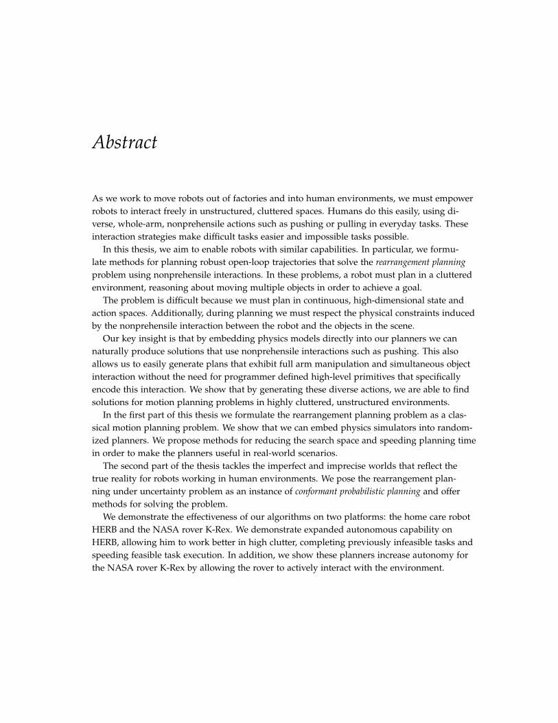
Abstract
As we work to move robots out of factories and into human environments, we must empowerrobots to interact freely in unstructured, cluttered spaces. Humans do this easily, using di-verse, whole-arm, nonprehensile actions such as pushing or pulling in everyday tasks. Theseinteraction strategies make difficult tasks easier and impossible tasks possible.
In this thesis, we aim to enable robots with similar capabilities. In particular, we formu-late methods for planning robust open-loop trajectories that solve the rearrangement planning
problem using nonprehensile interactions. In these problems, a robot must plan in a clutteredenvironment, reasoning about moving multiple objects in order to achieve a goal.
The problem is difficult because we must plan in continuous, high-dimensional state andaction spaces. Additionally, during planning we must respect the physical constraints inducedby the nonprehensile interaction between the robot and the objects in the scene.
Our key insight is that by embedding physics models directly into our planners we cannaturally produce solutions that use nonprehensile interactions such as pushing. This alsoallows us to easily generate plans that exhibit full arm manipulation and simultaneous objectinteraction without the need for programmer defined high-level primitives that specificallyencode this interaction. We show that by generating these diverse actions, we are able to findsolutions for motion planning problems in highly cluttered, unstructured environments.
In the first part of this thesis we formulate the rearrangement planning problem as a clas-sical motion planning problem. We show that we can embed physics simulators into random-ized planners. We propose methods for reducing the search space and speeding planning timein order to make the planners useful in real-world scenarios.
The second part of the thesis tackles the imperfect and imprecise worlds that reflect thetrue reality for robots working in human environments. We pose the rearrangement plan-ning under uncertainty problem as an instance of conformant probabilistic planning and offermethods for solving the problem.
We demonstrate the effectiveness of our algorithms on two platforms: the home care robotHERB and the NASA rover K-Rex. We demonstrate expanded autonomous capability onHERB, allowing him to work better in high clutter, completing previously infeasible tasks andspeeding feasible task execution. In addition, we show these planners increase autonomy forthe NASA rover K-Rex by allowing the rover to actively interact with the environment.

Acknowledgments
First and foremost, I would like to thank my advisor, Sidd Srinivasa, for his countless hours ofdiscussion and whiteboard sessions. I have learned so much from him about robotics, criticalthinking and clear presentation. His lessons translate beyond academics and I will always feelgrateful that he took a chance on me. I will also always have a special love for Palatino font.
I am very fortunate to have such a respected and distinguished committee: Matt Mason,Max Likhachev, David Hsu and Terry Fong. Their guidance and feedback throughout mythesis work was invaluable and I am grateful for the opportunity to interact with and learnfrom each one of them.
Throughout my work on this degree, I have had several external collaborators that eachuniquely shaped my journey. I would like to offer special thanks to Terry Fong and the mem-bers of the Intelligent Robotics Group at NASA Ames Research Laboratories, especially VytasSunspiral and Michael Furlong, for all their help with the KRex rover. In addition, thank youto the visiting researchers in our lab – Joshua Haustein, Marco Cognetti, Carolina Loureiroand Stefania Pellegrinelli.
My experience throughout my Ph.D. was made infinitely better by the members of the Per-sonal Robotics Laboratory - Mehmet, Anca, Koval, Dellin, Pras, Shushman, Gilwoo, Shervin,Liz, Laura, Aaron Walsman, Aaron Johnson, Matt, Stefanos, Clint, Henny, Rosario, Shen, Ar-iana, Oren, Mike0, Mike1, Rachel and Vinitha. The motivation and inspiration you each pro-vided in immeasurable. But beyond that, you made even the most stressful times fun. Also,thank you to Jean Harpley, Keyla Cook and Suzanne Lyons Muth, without whom the RoboticsInstitute and the Personal Robotics Lab would not have functioned.
I am so very fortunate to be surrounded by an incredible set of friends and family. My par-ents, Eileen and Dennis, have been my biggest supporters throughout life. They taught meto work hard and persevere, both through their words and example. They gave me the confi-dence and encouragement to achieve anything. And they never let me quit. For that I am sothankful. Thank you to my sister, Annie, and brother-in-law, Roy, for the endless encourage-ment and for being the best siblings I could ever ask for. Finally, to Anne and Marin. Thankyou for your constant and consistent support and love and for always being there to celebratemy successes and pick me up after failures. You made this possible.
The material in this dissertation was supported by funding from the NASA Space Technology Research Fellowship
program (award NNX13AL61H), the National Science Foundation IIS (award 1409003), Toyota Motor Engineering and
Manufacturing (TEMA) and the Office of Naval Research.

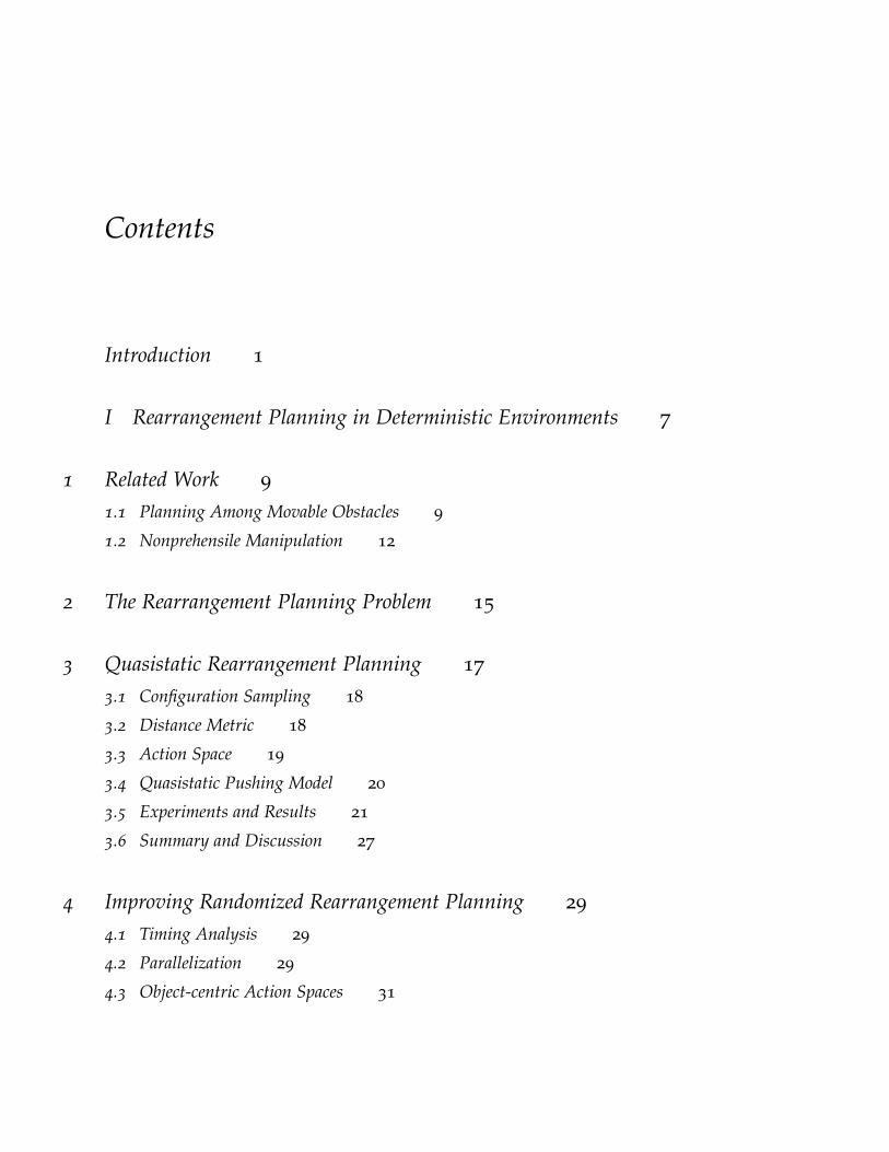
Contents
Introduction 1
I Rearrangement Planning in Deterministic Environments 7
1 Related Work 9
1.1 Planning Among Movable Obstacles 9
1.2 Nonprehensile Manipulation 12
2 The Rearrangement Planning Problem 15
3 Quasistatic Rearrangement Planning 17
3.1 Configuration Sampling 18
3.2 Distance Metric 18
3.3 Action Space 19
3.4 Quasistatic Pushing Model 20
3.5 Experiments and Results 21
3.6 Summary and Discussion 27
4 Improving Randomized Rearrangement Planning 29
4.1 Timing Analysis 29
4.2 Parallelization 29
4.3 Object-centric Action Spaces 31
8 jennifer e. king
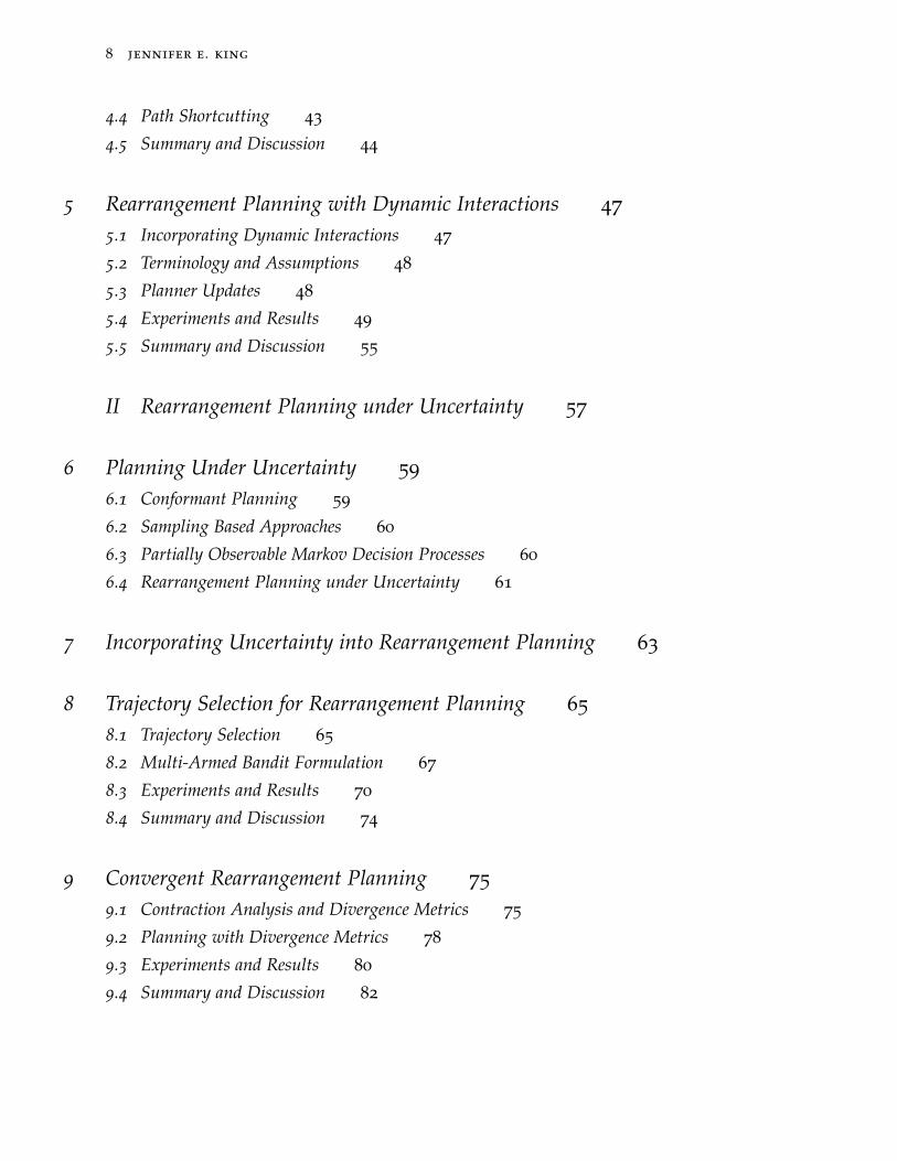
4.4 Path Shortcutting 43
4.5 Summary and Discussion 44
5 Rearrangement Planning with Dynamic Interactions 47
5.1 Incorporating Dynamic Interactions 47
5.2 Terminology and Assumptions 48
5.3 Planner Updates 48
5.4 Experiments and Results 49
5.5 Summary and Discussion 55
II Rearrangement Planning under Uncertainty 57
6 Planning Under Uncertainty 59
6.1 Conformant Planning 59
6.2 Sampling Based Approaches 60
6.3 Partially Observable Markov Decision Processes 60
6.4 Rearrangement Planning under Uncertainty 61
7 Incorporating Uncertainty into Rearrangement Planning 63
8 Trajectory Selection for Rearrangement Planning 65
8.1 Trajectory Selection 65
8.2 Multi-Armed Bandit Formulation 67
8.3 Experiments and Results 70
8.4 Summary and Discussion 74
9 Convergent Rearrangement Planning 75
9.1 Contraction Analysis and Divergence Metrics 75
9.2 Planning with Divergence Metrics 78
9.3 Experiments and Results 80
9.4 Summary and Discussion 82
robust rearrangement planning using nonprehensile interaction 9
10 Unobservable Monte Carlo Planning 83
10.1 Unobservable Markov Decision Processes 84
10.2 Monte Carlo Tree Search 85
10.3 Experiments and Results 90
10.4 Summary and Discussion 95
11 Conclusion 97
11.1 Lessons Learned 97
11.2 Future Work 98
11.3 The Last Word 101
A Rearrangement Planning via Heuristic Search 103
A.1 Action Selection 104
A.2 Heuristic 104
A.3 Expanding applicability 105
B Bibliography 117

Introduction
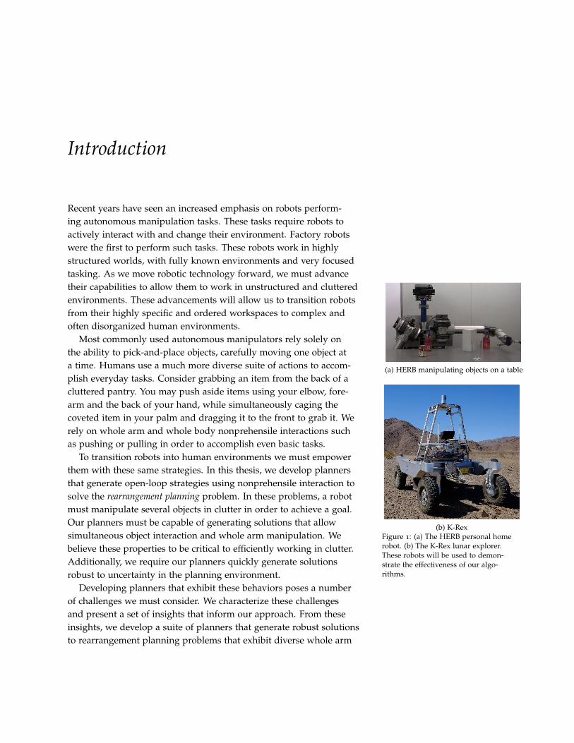
(a) HERB manipulating objects on a table
(b) K-RexFigure 1: (a) The HERB personal homerobot. (b) The K-Rex lunar explorer.These robots will be used to demon-strate the effectiveness of our algo-rithms.
Recent years have seen an increased emphasis on robots perform-ing autonomous manipulation tasks. These tasks require robots toactively interact with and change their environment. Factory robotswere the first to perform such tasks. These robots work in highlystructured worlds, with fully known environments and very focusedtasking. As we move robotic technology forward, we must advancetheir capabilities to allow them to work in unstructured and clutteredenvironments. These advancements will allow us to transition robotsfrom their highly specific and ordered workspaces to complex andoften disorganized human environments.
Most commonly used autonomous manipulators rely solely onthe ability to pick-and-place objects, carefully moving one object ata time. Humans use a much more diverse suite of actions to accom-plish everyday tasks. Consider grabbing an item from the back of acluttered pantry. You may push aside items using your elbow, fore-arm and the back of your hand, while simultaneously caging thecoveted item in your palm and dragging it to the front to grab it. Werely on whole arm and whole body nonprehensile interactions suchas pushing or pulling in order to accomplish even basic tasks.
To transition robots into human environments we must empowerthem with these same strategies. In this thesis, we develop plannersthat generate open-loop strategies using nonprehensile interaction tosolve the rearrangement planning problem. In these problems, a robotmust manipulate several objects in clutter in order to achieve a goal.Our planners must be capable of generating solutions that allowsimultaneous object interaction and whole arm manipulation. Webelieve these properties to be critical to efficiently working in clutter.Additionally, we require our planners quickly generate solutionsrobust to uncertainty in the planning environment.
Developing planners that exhibit these behaviors poses a numberof challenges we must consider. We characterize these challengesand present a set of insights that inform our approach. From theseinsights, we develop a suite of planners that generate robust solutionsto rearrangement planning problems that exhibit diverse whole arm
2
interactions.
Challenge 1: Integrating nonprehensile interactions. Nonprehensileinteractions have been shown to be critical for pre-grasp manipula-tion [29, 65], large object manipulation [33] and simultaneous objectinteraction [48, 64]. In addition, they can make manipulation possiblefor robots not traditionally designed for interaction tasks. Considerthe K-Rex robot from Fig.1b. Unless extra payload explicitely de-signed for performing manipulation tasks is added to the rover, thisrobot must rely on interactions such as pushing and toppling in or-der to manipulate the environment.
Purely geometric planners struggle to reason about nonprehensileinteraction because objects do not move rigidly with the robot. In-stead, the motion of objects evolves under non-holonomic constraintsthat represent the physics of the environment and the contact be-tween robot and objects. Our planning algorithms must respect thesemotion constraints.
Challenge 2: Fast planning in high-dimensional state and action spaces.
Our goal is to solve problems that require contact and interactionwith objects in the environment. This interaction changes the plan-ning environment. Because of this, we must track the objects therobot interacts with in our state during planning. This leads to asearch space size linear in the number of objects the manipulatorcan move. In addition, we wish to plan motions for a high degree-of-freedom (DOF) robot such as the HERB robot [115] (Fig.1a). Ourplanning algorithms must be capable of quickly planning in highdimensional state and action spaces.
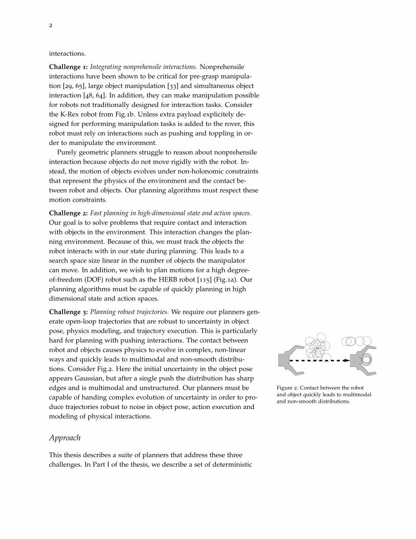
Challenge 3: Planning robust trajectories. We require our planners gen-erate open-loop trajectories that are robust to uncertainty in objectpose, physics modeling, and trajectory execution. This is particularlyhard for planning with pushing interactions. The contact betweenrobot and objects causes physics to evolve in complex, non-linearways and quickly leads to multimodal and non-smooth distribu-tions. Consider Fig.2. Here the initial uncertainty in the object poseappears Gaussian, but after a single push the distribution has sharpedges and is multimodal and unstructured. Our planners must becapable of handing complex evolution of uncertainty in order to pro-duce trajectories robust to noise in object pose, action execution andmodeling of physical interactions.
Figure 2: Contact between the robotand object quickly leads to multimodaland non-smooth distributions.
Approach
This thesis describes a suite of planners that address these threechallenges. In Part I of the thesis, we describe a set of deterministic
3
planners that solve rearrangement planning under the assumptionof perfect knowledge of the world and perfect modeling of robotmotions and interactions. These planners address the first two chal-lenges. We then augment these planners to allow us to address thethird challenge and handle the uncertainties prevalent when execut-ing tasks in the real world in Part II.
Randomized Rearrangement Planning in Deterministic Worlds
Randomized planners such as the Probabilistic Roadmap (PRM) [62]or Rapidly Exploring Random Tree (RRT) [76] have been shownto work well for high-dimensional state and action spaces. Theseplanners typically rely on being able to quickly solve the two-pointboundary value problem (BVP) to connect two states in state space.The use of pushing actions introduces non-holonomic constraints inthe planning problem that make solving the two-point BVP difficult.In particular, the motion of the pushed object is directly governedby the physics of the contact between robot and object. To empowerour planner to reason about object motion, we embed a physics model
into the core of a kinodynamic randomized planner [77]. This allows useliminate the need for simplifying assumption about object geometryand robot-object interaction prevalent in prior work [5, 15]. In thisthesis we demonstrate the use of both an analytic physics model withclosed form representation and commercial physics models such asBox2D [3].
We first formulate the problem under the quasistatic assump-tion (Ch.3). This increases tractability by allowing us to eliminatethe need to consider velocities in our search space, instead planningonly in configuration space. While this limits our solution space,the quasistatic assumption applies in many manipulation applica-tions [6, 7, 8, 24, 34, 89, 97, 129]. We show that we can reliably pro-duce solutions for multiple tasks including pushing objects to goallocations and clearing areas of clutter.
Even in this reduced state space the use of physics models withinour planner introduces extra computational complexity that slowsthe search. Additionally, our formulation in Ch.3 lacks goal-directedactions that explicitly aim to create the contact with objects criticalto rearrangement tasks. This further slows planning time. In Ch.4we demonstrate two techniques to regain speed. First, we show thatwe can increase the quantity of searched space by employing paral-lelization during tree growth. Second, we increase the quality of thesearch by improving the actions the planner considers. In particular,we show our framework is amenable to including motion primitivesprevalent in prior works [15, 36, 94]. By coupling these primitives
4
with our embedded physics model we strengthen their applicability,allowing them to demonstrate whole arm interaction with multipleobjects simultaneously. We demonstrate that allowing the planner to
consider both low-level robot motions and higher level object relative primi-
tives improves planning times and produces a powerful planner able tosolve many problems.
Limiting the search to quasistatic interactions allows us to managethe complexity of the search by planning only in configuration space.However, embedding physics models allows us to model dynamicinteractions such as striking an object and letting it slide. Naive in-tegration of these dynamic interactions into our planner doubles thesearch space by requiring incorporation of velocities into the state.This can have a crippling effect on the search time for our planner.We observe that for our problems the absence of any external forcesother than gravity causes a manipulated object to eventually come torest due to friction. In Ch.5, we show that we can use this observationto avoid the increased planning complexity by considering only dy-
namic actions that lead to statically stable states, i.e. we require all objectsin the scene to come to rest before the robot executes a new action.This increases the space of problems our planner can handle withonly minor penalties to planning time.
Robust Rearrangement Planning
The planners we present in Ch.3-Ch.5 allow us to solve rearrange-ment problems under perfect knowledge of the planning environ-ment. Such perfect conditions rarely exist. In the second half of thethesis we construct planners that consider the uncertainties prevalentin the real world. In Ch.8 we incorporate uncertainty by exploitingthe fact that each call to a randomized planner will generate a funda-mentally different trajectory and each generated trajectory varies inits likelihood to achieve the goal when executed in uncertain environ-ments. We formulate rearrangement planning under uncertainty as atrajectory selection problem. We use the planners developed in Part Ito generate several candidate trajectories. Then we describe a banditstyle algorithm to efficiently evaluate these candidates and select themost robust.
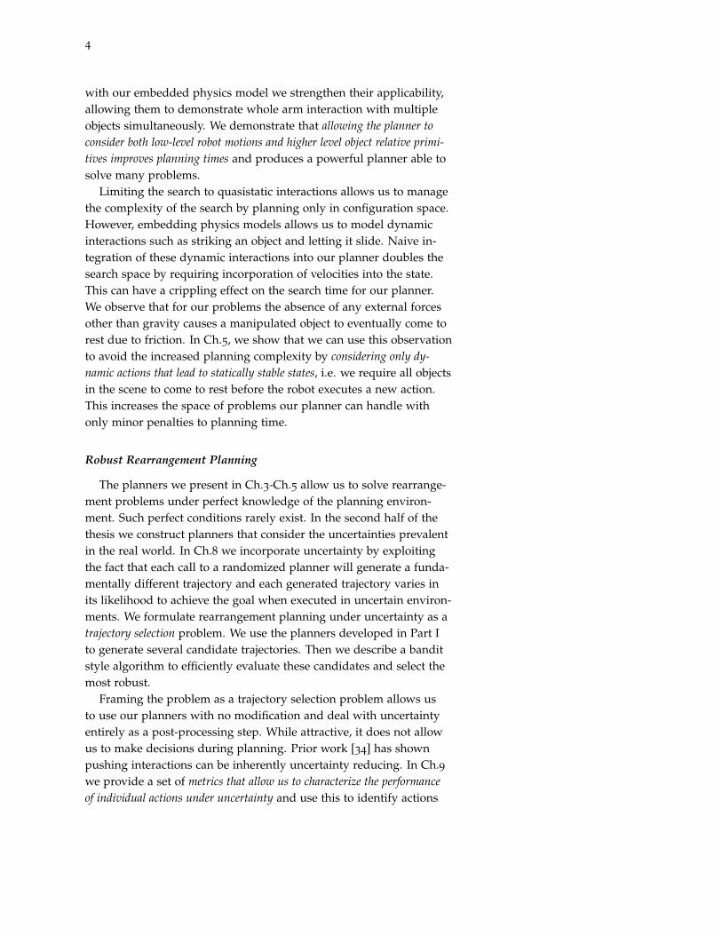
Framing the problem as a trajectory selection problem allows usto use our planners with no modification and deal with uncertaintyentirely as a post-processing step. While attractive, it does not allowus to make decisions during planning. Prior work [34] has shownpushing interactions can be inherently uncertainty reducing. In Ch.9we provide a set of metrics that allow us to characterize the performance
of individual actions under uncertainty and use this to identify actions
5
like the one pictured in Fig.3. We integrate these metrics into our ran-domized planning framework and show these allow us to producemore robust plans by handling uncertainty at plan time.
Figure 3: Non-prehensile interactionslike pushing can be inherent uncer-tainty reducing. Here a simple pushcollapsed initial uncertainty in the poseof the circular object.
This augmentation to our planner allows us to characterize per-formance of individual actions but does not consider the evolution ofuncertainty throughout sequences of actions. In Ch.10 we frame ourproblem as an instance of an Unobservable Markov Decision Process(UMDP). The nonprehensile interactions we consider lead to non-Gaussian and non-smooth distributions (Fig.2) that have no closedform representation. We leverage the physics model used duringplanning to perform Monte Carlo simulations of action sequences.This allows us to model the complicated evolution of uncertaintyinduced by the nonprehensile interaction. We show we can extendMonte Carlo algorithms for solving Markov Decision Precesses to theUMDP domain and use fast heuristic planners to quickly evaluate therobustness of action sequences. This allows us to produce trajectoriesthat perform well under real world uncertainties.
Contributions
In summary, we propose the following contributions in this thesis:
1. A kinodynamic randomized planner capable of solving complexrearrangement problems using nonprehensile interactions such aspushing.
2. A set of metrics that identify and measure the robustness of in-dividual actions and full rearrangement plans to uncertaintiesprevalent at execution time.
3. A set of methods that use Monte Carlo simulations to estimatethese metrics, allowing us to identify and generate robust open-loop rearrangement plans.
4. Experimental validation of our developed planners against state-of-the-art baseline approaches on multiple platforms.
Pla
nn
ing
Tim
e
Implementation Complexity
Ch.3
Ch.4
Ch.5
Ch.8
Ch.9Ch.10
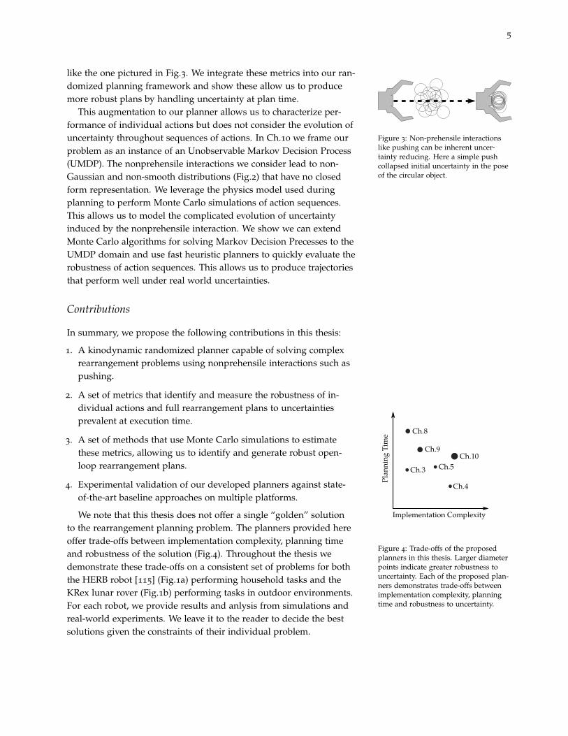
Figure 4: Trade-offs of the proposedplanners in this thesis. Larger diameterpoints indicate greater robustness touncertainty. Each of the proposed plan-ners demonstrates trade-offs betweenimplementation complexity, planningtime and robustness to uncertainty.
We note that this thesis does not offer a single “golden” solutionto the rearrangement planning problem. The planners provided hereoffer trade-offs between implementation complexity, planning timeand robustness of the solution (Fig.4). Throughout the thesis wedemonstrate these trade-offs on a consistent set of problems for boththe HERB robot [115] (Fig.1a) performing household tasks and theKRex lunar rover (Fig.1b) performing tasks in outdoor environments.For each robot, we provide results and anlysis from simulations andreal-world experiments. We leave it to the reader to decide the bestsolutions given the constraints of their individual problem.

Part I
Rearrangement Planning in
Deterministic
Environments

1
Related Work
This work lies at the intersection of planning among movable obstacles
and nonprehensile manipulation. We provide an overview of relatedwork in each of these individual fields.
1.1 Planning Among Movable Obstacles
We wish to perform tasks that require the robot to work in clutter.To achieve such tasks robots must be able to reason about movingmultiple objects. Wilfong [125] was the first to show that problemsof this type are NP-hard. However, it has been shown that imposingsimplifying assumptions can make the problem tractable.
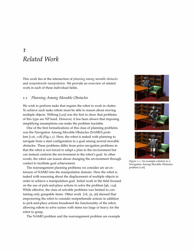
Figure 1.1: An example solution to aNavigation Among Movable Obstaclesproblem [116]
One of the first formalizations of this class of planning problemswas the Navigation Among Movable Obstacles (NAMO) prob-lem [116, 118] (Fig.1.1). Here, the robot is tasked with planning tonavigate from a start configuration to a goal among several movableobstacles. These problems differ from prior navigation problems inthat the robot is not forced to adapt a plan to the environment butcan instead conform the environment to the robot’s goal. In otherwords, the robot can reason about changing the environment throughcontact to facilitate goal achievement.
The rearrangement planning problems we consider are an ex-tension of NAMO into the manipulation domain. Here the robot istasked with reasoning about the displacement of multiple objects inorder to achieve a manipulation goal. Initial work in the field focusedon the use of pick-and-place actions to solve the problem [96, 119].While effective, the class of solvable problems was limited to con-taining only graspable items. Other work [18, 35, 36] showed thatempowering the robot to consider nonprehensile actions in additionto pick-and-place actions broadened the functionality of the robot,allowing robots to solve scenes with items too large or heavy for therobot to grasp.
The NAMO problem and the rearrangement problem are example
10 robust rearrangement planning using nonprehensile interaction
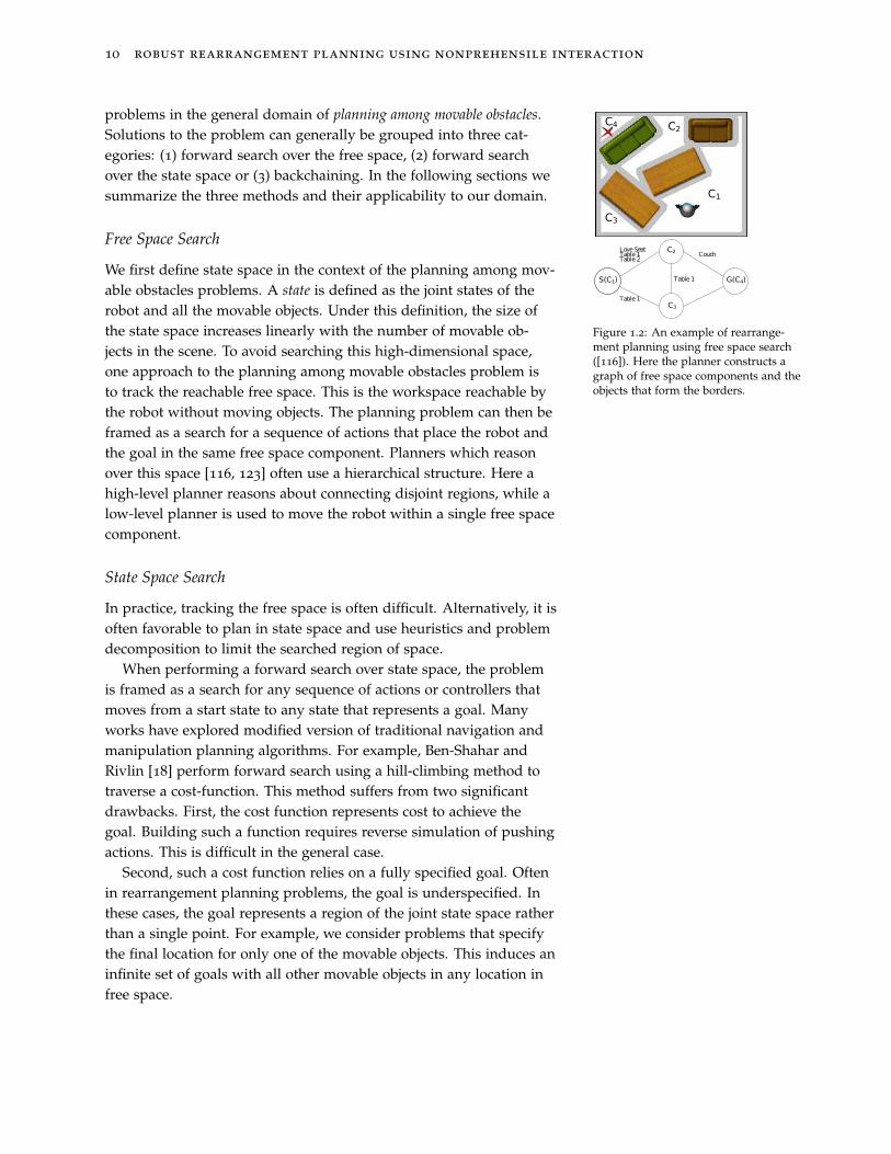
problems in the general domain of planning among movable obstacles.Solutions to the problem can generally be grouped into three cat-egories: (1) forward search over the free space, (2) forward searchover the state space or (3) backchaining. In the following sections wesummarize the three methods and their applicability to our domain.
Free Space Search
C1
C2
C3
C4
S(C1) G(C4)
C2
C3
LoveSeatTable1Table2
Table1
Table1
Couch
Figure 1.2: An example of rearrange-ment planning using free space search([116]). Here the planner constructs agraph of free space components and theobjects that form the borders.
We first define state space in the context of the planning among mov-able obstacles problems. A state is defined as the joint states of therobot and all the movable objects. Under this definition, the size ofthe state space increases linearly with the number of movable ob-jects in the scene. To avoid searching this high-dimensional space,one approach to the planning among movable obstacles problem isto track the reachable free space. This is the workspace reachable bythe robot without moving objects. The planning problem can then beframed as a search for a sequence of actions that place the robot andthe goal in the same free space component. Planners which reasonover this space [116, 123] often use a hierarchical structure. Here ahigh-level planner reasons about connecting disjoint regions, while alow-level planner is used to move the robot within a single free spacecomponent.
State Space Search
In practice, tracking the free space is often difficult. Alternatively, it isoften favorable to plan in state space and use heuristics and problemdecomposition to limit the searched region of space.
When performing a forward search over state space, the problemis framed as a search for any sequence of actions or controllers thatmoves from a start state to any state that represents a goal. Manyworks have explored modified version of traditional navigation andmanipulation planning algorithms. For example, Ben-Shahar andRivlin [18] perform forward search using a hill-climbing method totraverse a cost-function. This method suffers from two significantdrawbacks. First, the cost function represents cost to achieve thegoal. Building such a function requires reverse simulation of pushingactions. This is difficult in the general case.
Second, such a cost function relies on a fully specified goal. Oftenin rearrangement planning problems, the goal is underspecified. Inthese cases, the goal represents a region of the joint state space ratherthan a single point. For example, we consider problems that specifythe final location for only one of the movable objects. This induces aninfinite set of goals with all other movable objects in any location infree space.
related work 11
Other solutions follow the terminology for manipulation plan-ning introduced by Simeon et. al. [112] and structure the problem asreasoning over two types of action classes:
• Transit - The robot moves on its own, without making contact withany movable objects
• Transfer - The robot manipulates one or more movable objects
Then the problem becomes searching for a sequence of transit andtransfer actions that lead to a goal state. Such problems can be solvedusing search algorithms suitable for high dimensional problems, suchas the RRT. Tractibility is maintained by limiting search to alternatingsequences of transit and transfer actions [96].
Further tractibility of the problem can be gained by decomposingthe full problem into a sequence of subgoals involving subsets of ob-jects [17, 31, 72, 99]. However, such decomposition explicitly forbidsmulti-object contact, eliminating a large set of feasible solutions.
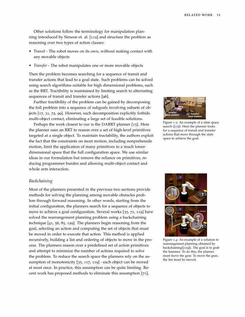
Figure 1.3: An example of a state spacesearch ([15]). Here the planner looksfor a sequence of transit and transferactions that move through the statespace to achieve the goal.
Perhaps the work closest to our is the DARRT planner [15]. Herethe planner uses an RRT to reason over a set of high-level primitivestargeted at a single object. To maintain tractability, the authors exploitthe fact that the constraints on most motion, including nonprehensilemotion, limit the application of many primitives to a much lower-dimensional space that the full configuration space. We use similarideas in our formulation but remove the reliance on primitives, re-ducing programmer burden and allowing multi-object contact andwhole arm interaction.
Backchaining
Figure 1.4: An example of a solution torearrangement planning obtained bybackchaining([119]). The goal is to grabthe hammer. To do this, the plannermust move the gear. To move the gear,the fan must be moved.
Most of the planners presented in the previous two sections providemethods for solving the planning among movable obstacles prob-lem through forward reasoning. In other words, starting from theinitial configuration, the planners search for a sequence of objects tomove to achieve a goal configuration. Several works [35, 71, 119] havesolved the rearrangement planning problem using a backchainingtechnique [41, 56, 85, 129]. The planners begin reasoning from thegoal, selecting an action and computing the set of objects that mustbe moved in order to execute that action. This method is appliedrecursively, building a list and ordering of objects to move in the pro-cess. The planners reason over a predefined set of action primitivesand attempt to minimize the number of actions required to solvethe problem. To reduce the search space the planners rely on the as-sumption of monotonicity [35, 117, 119] - each object can be movedat most once. In practice, this assumption can be quite limiting. Re-cent work has proposed methods to eliminate this assumption [71],
12 robust rearrangement planning using nonprehensile interaction
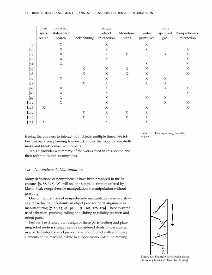
Freespacesearch
Forwardstate-space
search Backchaining
Singleobject
interactionMonotone
plansContact
primitives
Fullyspecified
goalNonprehensile
interaction
[9] X X X[15] X X X X[17] X X X X X[18] X X X[31] X X X[35] X X X X X[36] X X X X X[72] X X X X[71] X X X X[94] X X X X[96] X X X[99] X X X X
[112] X X X X[116] X X X X[117] X X X X[119] X X X X[123] X X X
Table 1.1: Planning among movableobjectsfreeing the planners to interact with objects multiple times. We fol-
low this lead: our planning framework allows the robot to repeatedlymake and break contact with objects.
Tab.1.1 provides a summary of the works cited in this section andtheir techniques and assumptions.
1.2 Nonprehensile Manipulation
Many definitions of nonprehensile have been proposed in the lit-erature [5, 88, 128]. We will use the simple definition offered byMason [92]: nonprehensile manipulation is manipulation withoutgrasping.
One of the first uses of nonprehensile manipulation was as a strat-egy for reducing uncertainty in object pose for parts alignment inmanufacturing [7, 21, 23, 42, 40, 46, 54, 103, 128, 129]. These systemsused vibration, pushing, rolling and sliding to reliably position andorient parts.
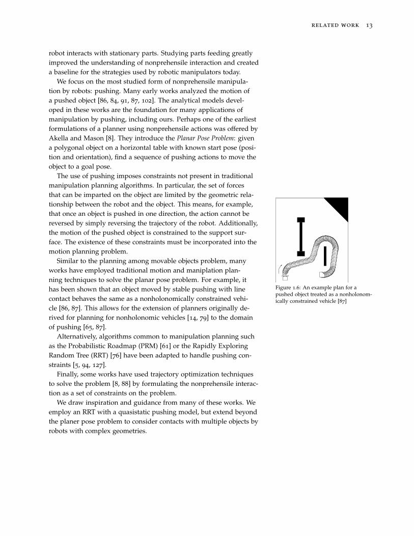
Figure 1.5: Example parts feeder usingstationary fences to align objects [103]
Peshkin [103] noted that design of these parts-feeding and plan-ning robot motion strategy can be considered duals to one another:in a parts-feeder the workpieces move and interact with stationaryelements of the machine, while in a robot motion plan the moving
related work 13
robot interacts with stationary parts. Studying parts feeding greatlyimproved the understanding of nonprehensile interaction and createda baseline for the strategies used by robotic manipulators today.
We focus on the most studied form of nonprehensile manipula-tion by robots: pushing. Many early works analyzed the motion ofa pushed object [86, 84, 91, 87, 102]. The analytical models devel-oped in these works are the foundation for many applications ofmanipulation by pushing, including ours. Perhaps one of the earliestformulations of a planner using nonprehensile actions was offered byAkella and Mason [8]. They introduce the Planar Pose Problem: givena polygonal object on a horizontal table with known start pose (posi-tion and orientation), find a sequence of pushing actions to move theobject to a goal pose.
The use of pushing imposes constraints not present in traditionalmanipulation planning algorithms. In particular, the set of forcesthat can be imparted on the object are limited by the geometric rela-tionship between the robot and the object. This means, for example,that once an object is pushed in one direction, the action cannot bereversed by simply reversing the trajectory of the robot. Additionally,the motion of the pushed object is constrained to the support sur-face. The existence of these constraints must be incorporated into themotion planning problem.
Figure 1.6: An example plan for apushed object treated as a nonholonom-ically constrained vehicle [87]
Similar to the planning among movable objects problem, manyworks have employed traditional motion and maniplation plan-ning techniques to solve the planar pose problem. For example, ithas been shown that an object moved by stable pushing with linecontact behaves the same as a nonholonomically constrained vehi-cle [86, 87]. This allows for the extension of planners originally de-rived for planning for nonholonomic vehicles [14, 79] to the domainof pushing [65, 87].
Alternatively, algorithms common to manipulation planning suchas the Probabilistic Roadmap (PRM) [61] or the Rapidly ExploringRandom Tree (RRT) [76] have been adapted to handle pushing con-straints [5, 94, 127].
Finally, some works have used trajectory optimization techniquesto solve the problem [8, 88] by formulating the nonprehensile interac-tion as a set of constraints on the problem.
We draw inspiration and guidance from many of these works. Weemploy an RRT with a quasistatic pushing model, but extend beyondthe planer pose problem to consider contacts with multiple objects byrobots with complex geometries.

2
The Rearrangement Planning Problem R RobotXR Robot state spaceM Movable objectsXi Movable i state spaceO Static obstaclesX Planning state space
X f ree Free state spaceXG Goal regionU Control spaceξ Feasible trajectoryπ Control sequence
Table 2.1: Rearrangement planningterminology
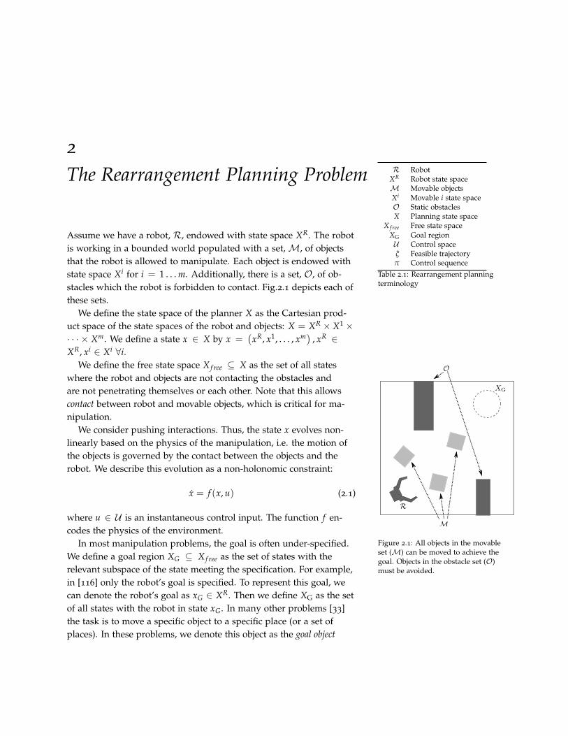
Figure 2.1: All objects in the movableset (M) can be moved to achieve thegoal. Objects in the obstacle set (O)must be avoided.
Assume we have a robot, R, endowed with state space XR. The robotis working in a bounded world populated with a set,M, of objectsthat the robot is allowed to manipulate. Each object is endowed withstate space Xi for i = 1 . . . m. Additionally, there is a set, O, of ob-stacles which the robot is forbidden to contact. Fig.2.1 depicts each ofthese sets.
We define the state space of the planner X as the Cartesian prod-uct space of the state spaces of the robot and objects: X = XR × X1 ×
· · · × Xm. We define a state x ∈ X by x =(xR, x1, . . . , xm
), xR ∈
XR, xi ∈ Xi ∀i.We define the free state space X f ree ⊆ X as the set of all states
where the robot and objects are not contacting the obstacles andare not penetrating themselves or each other. Note that this allowscontact between robot and movable objects, which is critical for ma-nipulation.
We consider pushing interactions. Thus, the state x evolves non-linearly based on the physics of the manipulation, i.e. the motion ofthe objects is governed by the contact between the objects and therobot. We describe this evolution as a non-holonomic constraint:
x = f (x, u) (2.1)
where u ∈ U is an instantaneous control input. The function f en-codes the physics of the environment.
In most manipulation problems, the goal is often under-specified.We define a goal region XG ⊆ X f ree as the set of states with therelevant subspace of the state meeting the specification. For example,in [116] only the robot’s goal is specified. To represent this goal, wecan denote the robot’s goal as xG ∈ XR. Then we define XG as the setof all states with the robot in state xG. In many other problems [33]the task is to move a specific object to a specific place (or a set ofplaces). In these problems, we denote this object as the goal object

16 robust rearrangement planning using nonprehensile interaction
G ∈ M with its state space XG and its goal as the set G ⊆ XG. Wedefine XG ⊆ X f ree as the set of all states with the goal object in G.
The task of the rearrangement planning problem is to find a fea-sible trajectory ξ : R
≥0 → X f ree starting from a state ξ(0) ∈ X f ree
and ending in a goal region ξ(T) ∈ XG ⊆ X f ree at some time T ≥ 0.A path ξ is feasible if there exists a mapping π : R
≥0 → U suchthat ξ(t) = f (ξ(t), π(t)) for all t ≥ 0. This requirement ensures wecan satisfy the constraint f while following ξ by executing the con-trols dictated by π. Tab.2.1 provides a summary of the terminologyintroduced in this section.

3
Quasistatic Rearrangement Planning
This chapter is adapted from King etal. [64].We utilize a Rapidly Exploring Random Tree (RRT) [76] to solve the
rearrangement problem. The basic RRT algorithm iteratively buildsa tree with nodes representing states in X f ree and edges representingactions or motions of the system through X f ree. Tree building pro-ceeds in four steps: (1) sample a random state xrand ∈ X f ree (Fig.3.1a),(2) locate the nearest node in the tree xnear under a distance met-ric, (3) select a control, u ∈ U that minimizes distance from xnear
to xrand while remaining in X f ree (Fig.3.1b), (4) add xnew, the statereached by applying u, and the edge connecting xnear to xnew to thetree (Fig.3.1c). The algorithm iterates until a node is added to thetree that represents a goal state x ∈ XG. RRTs have been shown tobe well suited for planning in high dimensional state spaces withnon-holonomic constraints, making them an ideal fit for our problem.
Because we must plan in the joint configuration space of the robotand objects, selecting the control u that exactly minimizes the dis-tance from xnear to xrand is as difficult as solving the full problem. Forexample, consider the extension in Fig.3.1. To transition from xnear
to xrand, we must first find a collision free path for the manipulatorfrom its configuration in xnear to a location near the object. Then wemust find a path that pushes the object to its new location. Finally,we must generate a collision free path to move the manipulator toits configuration in xrand. As the number of objects in the scene in-creases, the complexity of finding these sequences that connect twostates in X f ree grows exponentially.
As suggested by Lavalle [77] a useful alternative is to use a dis-crete time approximation to Eq.(2.1) to forward propagate all possiblecontrols and select the best using a distance metric defined on thestate space. In particular, we define an action set A : U ×R
≥0 wherea = (u, d) ∈ A describes a control, u, and associated duration, d, toapply the control. Then we use a transition function Γ : X ×A → X
to approximate our non-holonomic constraint.Our control space U is continuous, rendering full enumeration of
18 robust rearrangement planning using nonprehensile interaction
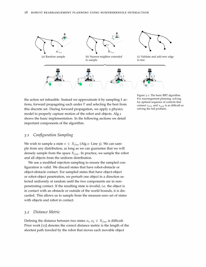
xrand
(a) Random sample
xrand
xnear
(b) Nearest neighbor extendedto sample
(c) Validate and add new edgeto tree
︷ ︸︸ ︷
Figure 3.1: The basic RRT algorithm.For rearrangement planning, solvingfor optimal sequence of controls thatconnect xnear and xrand is as difficult assolving the full problem.
the action set infeasible. Instead we approximate it by sampling k ac-tions, forward propagating each under Γ and selecting the best fromthis discrete set. During forward propagation, we apply a physicsmodel to properly capture motion of the robot and objects. Alg.1shows the basic implementation. In the following sections we detailimportant components of the algorithm.
3.1 Configuration Sampling
We wish to sample a state x ∈ X f ree (Alg.1- Line 3). We can sam-ple from any distribution, as long as we can guarantee that we willdensely sample from the space X f ree. In practice, we sample the robotand all objects from the uniform distribution.
We use a modified rejection sampling to ensure the sampled con-figuration is valid. We discard states that have robot-obstacle orobject-obstacle contact. For sampled states that have object-objector robot-object penetration, we perturb one object in a direction se-lected uniformly at random until the two components are in non-penetrating contact. If the resulting state is invalid, i.e. the object isin contact with an obstacle or outside of the world bounds, it is dis-carded. This allows us to sample from the measure-zero set of stateswith objects and robot in contact.
3.2 Distance Metric
Defining the distance between two states x1, x2 ∈ X f ree is difficult.Prior work [15] denotes the correct distance metric is the length of theshortest path traveled by the robot that moves each movable object
quasistatic rearrangement planning 19
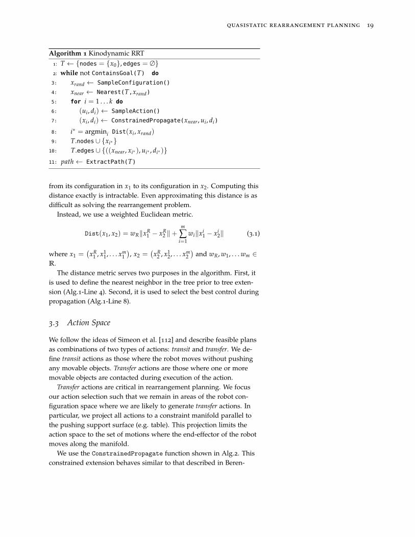
Algorithm 1 Kinodynamic RRT
1: T ← {nodes = {x0}, edges = ∅}
2: while not ContainsGoal(T) do
3: xrand ← SampleConfiguration()
4: xnear ← Nearest(T,xrand)
5: for i = 1 . . . k do
6: (ui, di)← SampleAction()
7: (xi, di)← ConstrainedPropagate(xnear, ui, di)
8: i∗ = argmini Dist(xi, xrand)
9: T.nodes∪ {xi∗}
10: T.edges∪ {((xnear, xi∗), ui∗ , di∗)}
11: path← ExtractPath(T)
from its configuration in x1 to its configuration in x2. Computing thisdistance exactly is intractable. Even approximating this distance is asdifficult as solving the rearrangement problem.
Instead, we use a weighted Euclidean metric.
Dist(x1, x2) = wR‖xR1 − xR
2 ‖+m
∑i=1
wi‖xi1 − xi
2‖ (3.1)
where x1 =(
xR1 , x1
1, . . . xm1
), x2 =
(xR
2 , x12, . . . xm
2
)and wR, w1, . . . wm ∈
R.The distance metric serves two purposes in the algorithm. First, it
is used to define the nearest neighbor in the tree prior to tree exten-sion (Alg.1-Line 4). Second, it is used to select the best control duringpropagation (Alg.1-Line 8).
3.3 Action Space
We follow the ideas of Simeon et al. [112] and describe feasible plansas combinations of two types of actions: transit and transfer. We de-fine transit actions as those where the robot moves without pushingany movable objects. Transfer actions are those where one or moremovable objects are contacted during execution of the action.
Transfer actions are critical in rearrangement planning. We focusour action selection such that we remain in areas of the robot con-figuration space where we are likely to generate transfer actions. Inparticular, we project all actions to a constraint manifold parallel tothe pushing support surface (e.g. table). This projection limits theaction space to the set of motions where the end-effector of the robotmoves along the manifold.
We use the ConstrainedPropagate function shown in Alg.2. Thisconstrained extension behaves similar to that described in Beren-
20 robust rearrangement planning using nonprehensile interaction
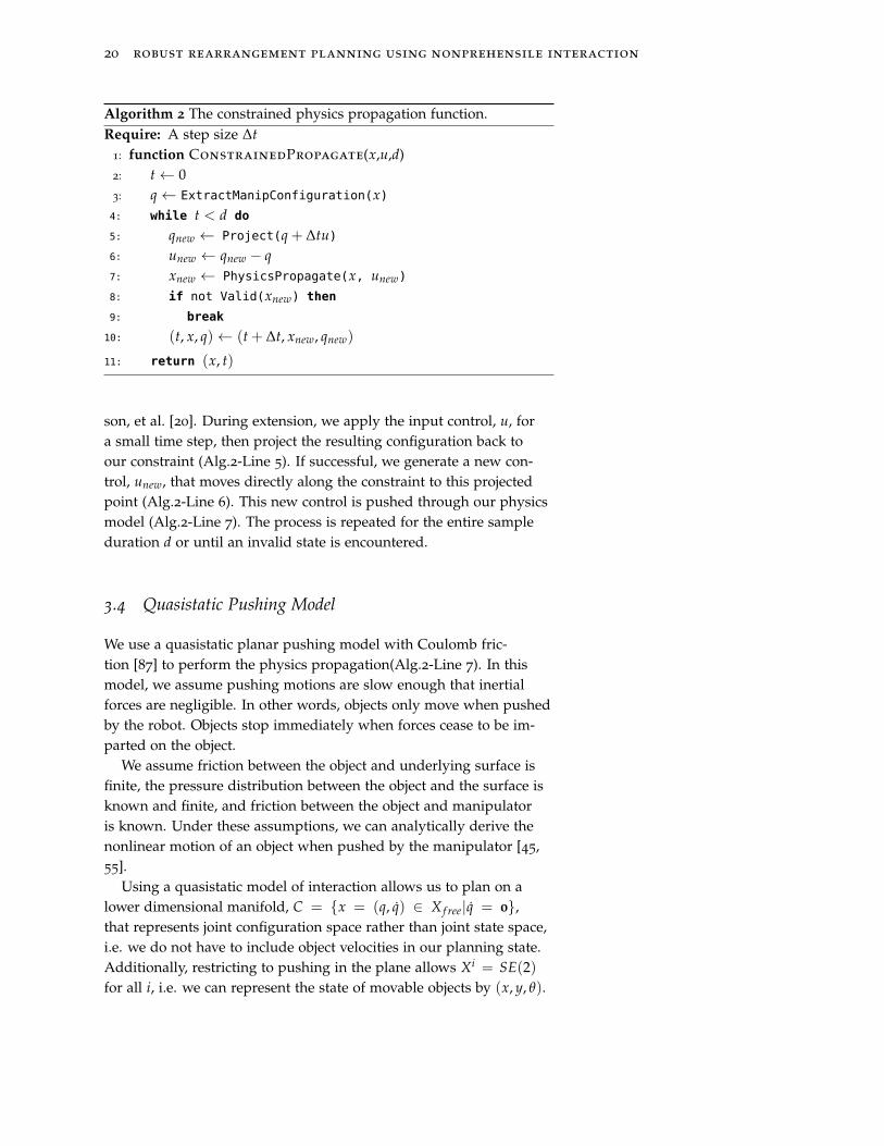
Algorithm 2 The constrained physics propagation function.Require: A step size ∆t
1: function ConstrainedPropagate(x,u,d)2: t← 03: q← ExtractManipConfiguration(x)
4: while t < d do
5: qnew ← Project(q + ∆tu)
6: unew ← qnew − q
7: xnew ← PhysicsPropagate(x, unew)
8: if not Valid(xnew) then
9: break
10: (t, x, q)← (t + ∆t, xnew, qnew)
11: return (x, t)
son, et al. [20]. During extension, we apply the input control, u, fora small time step, then project the resulting configuration back toour constraint (Alg.2-Line 5). If successful, we generate a new con-trol, unew, that moves directly along the constraint to this projectedpoint (Alg.2-Line 6). This new control is pushed through our physicsmodel (Alg.2-Line 7). The process is repeated for the entire sampleduration d or until an invalid state is encountered.
3.4 Quasistatic Pushing Model
We use a quasistatic planar pushing model with Coulomb fric-tion [87] to perform the physics propagation(Alg.2-Line 7). In thismodel, we assume pushing motions are slow enough that inertialforces are negligible. In other words, objects only move when pushedby the robot. Objects stop immediately when forces cease to be im-parted on the object.
We assume friction between the object and underlying surface isfinite, the pressure distribution between the object and the surface isknown and finite, and friction between the object and manipulatoris known. Under these assumptions, we can analytically derive thenonlinear motion of an object when pushed by the manipulator [45,55].
Using a quasistatic model of interaction allows us to plan on alower dimensional manifold, C = {x = (q, q) ∈ X f ree|q = 0},that represents joint configuration space rather than joint state space,i.e. we do not have to include object velocities in our planning state.Additionally, restricting to pushing in the plane allows Xi = SE(2)for all i, i.e. we can represent the state of movable objects by (x, y, θ).

quasistatic rearrangement planning 21
3.5 Experiments and Results
We implement the algorithm by extending the Open Motion PlanningLibrary (OMPL) framework [120]. We test our algorithm for threegoals: 1. Push an object to a goal region, 2. Move the manipulatorto a goal region, 3. Clear a region of all objects. In the followingsections, we present results and analysis from simulation experimentsfor each of these three goals. We then present results from executionof the planned paths in the real world.
3.5.1 Push object
Figure 3.2: An example task. HERBmust push the green box along the tableinto the region denoted by the greencircle.
In our first set of experiments, we task our robot HERB [115] withpushing an object (denoted “goal object”) on a table to a goal regionof radius 0.1 m using the 7-DOF left arm. We test our planner usinga dataset consisting of 7 randomly generated scenes with between1 and 7 movable objects in the robot’s reachable workspace. Fig.3.2shows an example scene. In each scene, we use the same goal object.The starting pose of the goal object is randomly selected. The goalregion is placed in the same location across all scenes. We run eachexperiment 50 times, giving us a total of 350 trials. A trial is consid-ered successful if a solution is found within 300 seconds.
We constrain the end-effector to move in the xy-plane parallel tothe table. This allows us to define our action space as the space offeasible velocities for the end-effector. Actions are uniformly sampledfrom a bounded range. The Project function takes the sampled end-effector velocity and generates an updated pose using the Jacobianpseudoinverse:
qnew = q + ∆t(J†(q)a + h(q)) (3.2)
where q is the current arm configuration, a is the sampled end-effector velocity and h : R
7 → R7 is a function that samples the
nullspace.
Comparison with baseline planners
We denote our planner Physics Constrained RRT (PC RRT) andcompare its performance against two baseline planners. The firstplanner (denoted Static RRT in all results) only allows the robot topush the goal object. All other movable objects are treated as staticobstacles. Comparing with this planning scheme allows us to exploreour first hypothesis:
H.1 Allowing the planner to move clutter increases success rateand decreases plan time.
22 robust rearrangement planning using nonprehensile interaction
H.1 is motivated by two purposes. First, previous work has demon-strated that allowing the manipulator to move clutter increases thenumber of problems that can be solved [33, 48]. We verify our plan-ner is consistent with these results. Second, we ensure that the extratime required to propagate with the physics model is not so largethat the planner can no longer generate feasible solutions in a reason-able amount of time.
We also compare our planner to an implementation of DARRT [15].Following DARRT, we define three primitives:
1. Transit - Move the manipulator from one pose to another via astraight line in configuration space. The motion must be free ofcollision with any static or movable object in the space.
2. RRTTransit - Move the manipulator from one configuration toanother by planning using the RRT-Connect algorithm [73]. Themotion must be free of collision with any static or movable objectin the scene. The planner is run for 5 seconds before the primitiveis considered failed.
3. Push - Push (or pull) an object along a straight line from the startpose to the goal pose of the object. The object motion is modeledas a rigid connection with the hand. Again, the motion must befree of collision with any static objects and all movable objectsother than the one being moved.
At each iteration, DARRT chooses to either sample a new pose forthe manipulator or a new pose for a single movable object. In ourimplementation, we sample these options with equal probability.
If the manipulator is sampled, then the planner attempts to ap-ply the Transit or RRTTransit primitive. If any of the objects aresampled, the RRTTransit primitive is first applied to move the ma-nipulator to make contact between the end-effector (hand) and object.Then, the Push primitive is applied to relocate the object to its de-sired position.
Comparing with this existing state-of-the-art rearrangement plan-ner allows us to explore a second hypothesis:
H.2 Our algorithm increases success rate and decreases planningtime when compared to existing primitive based solutions.
Parameter selection
We identify three parameters that can affect performance of thealgorithm. The first is pgoal , the probability that the sample state
quasistatic rearrangement planning 23
Forearm
Wrist
Finger2
Finger1
Time(a) (b) (c) (d) (e)
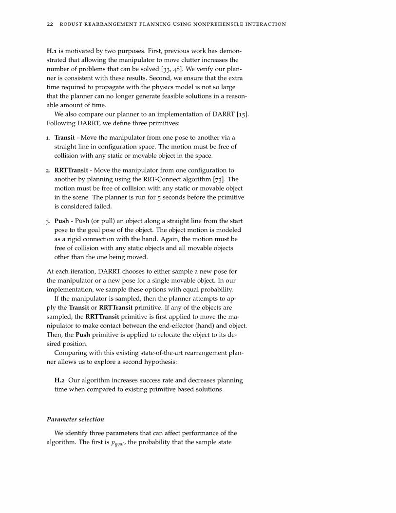
(a) (b) (c) (d) (e)Figure 3.4: In this scene the robot usesthe whole arm to manipulate objects toachieve the goal. At several time points((c), (d), (e)), the robot moves multipleobjects simultaneously.
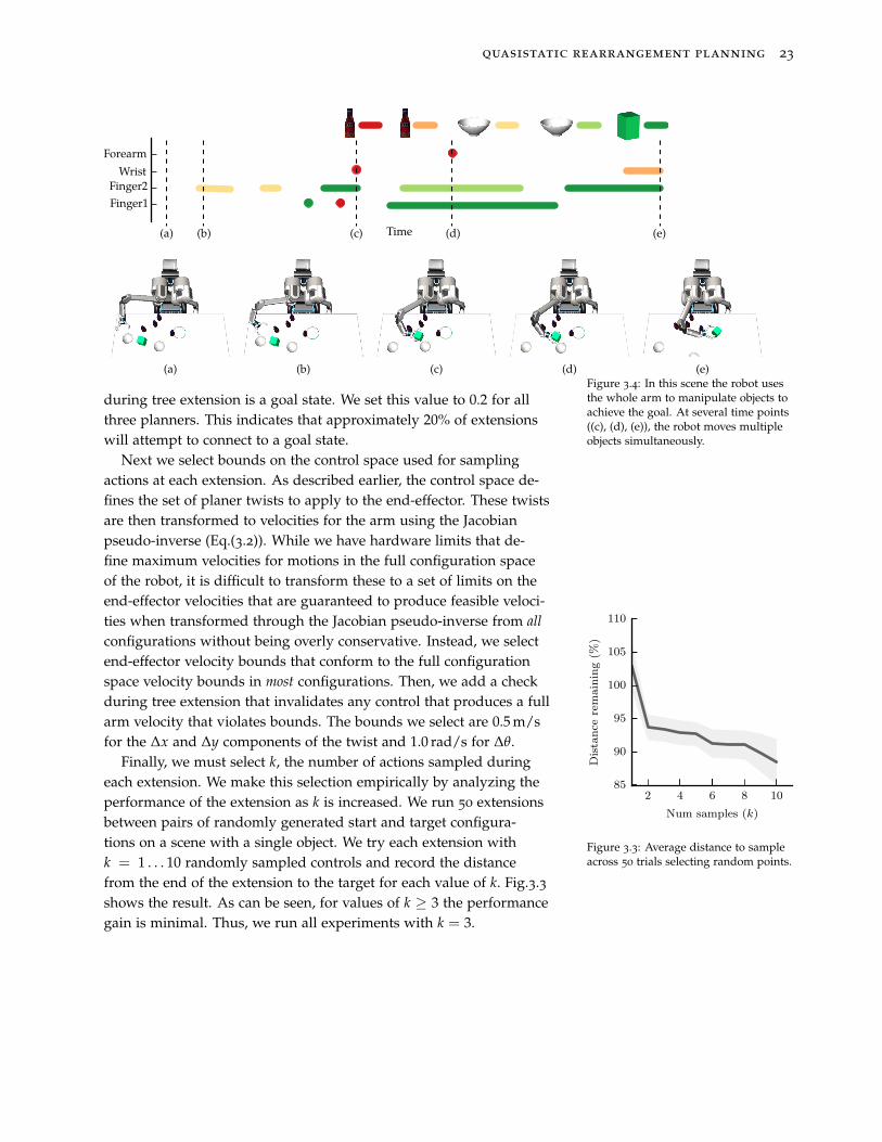
during tree extension is a goal state. We set this value to 0.2 for allthree planners. This indicates that approximately 20% of extensionswill attempt to connect to a goal state.
Next we select bounds on the control space used for samplingactions at each extension. As described earlier, the control space de-fines the set of planer twists to apply to the end-effector. These twistsare then transformed to velocities for the arm using the Jacobianpseudo-inverse (Eq.(3.2)). While we have hardware limits that de-fine maximum velocities for motions in the full configuration spaceof the robot, it is difficult to transform these to a set of limits on theend-effector velocities that are guaranteed to produce feasible veloci-ties when transformed through the Jacobian pseudo-inverse from all
configurations without being overly conservative. Instead, we selectend-effector velocity bounds that conform to the full configurationspace velocity bounds in most configurations. Then, we add a checkduring tree extension that invalidates any control that produces a fullarm velocity that violates bounds. The bounds we select are 0.5 m/sfor the ∆x and ∆y components of the twist and 1.0 rad/s for ∆θ.
2 4 6 8 10
Num samples (k)
85
90
95
100
105
110
Distance
remaining(%
)
Figure 3.3: Average distance to sampleacross 50 trials selecting random points.
Finally, we must select k, the number of actions sampled duringeach extension. We make this selection empirically by analyzing theperformance of the extension as k is increased. We run 50 extensionsbetween pairs of randomly generated start and target configura-tions on a scene with a single object. We try each extension withk = 1 . . . 10 randomly sampled controls and record the distancefrom the end of the extension to the target for each value of k. Fig.3.3shows the result. As can be seen, for values of k ≥ 3 the performancegain is minimal. Thus, we run all experiments with k = 3.
24 robust rearrangement planning using nonprehensile interaction
Elbow
Forearm
WristFinger2Finger1
Time(a) (b) (c) (d) (e)
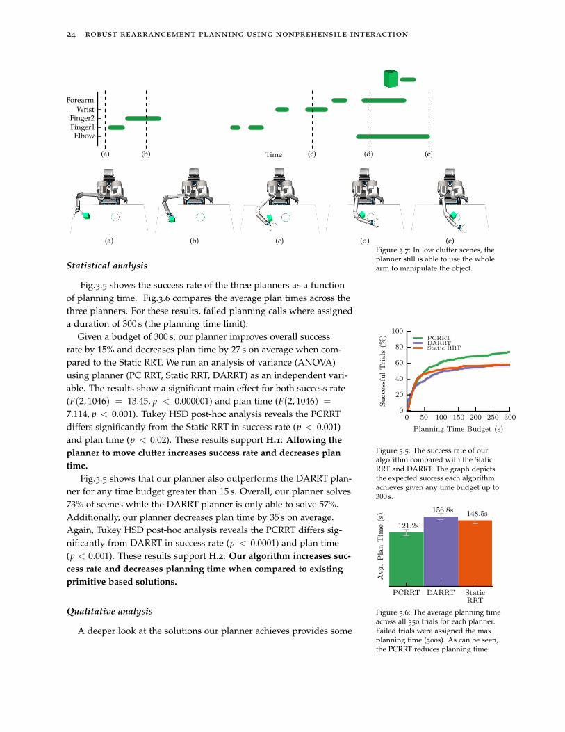
(a) (b) (c) (d) (e)Figure 3.7: In low clutter scenes, theplanner still is able to use the wholearm to manipulate the object.Statistical analysis
Fig.3.5 shows the success rate of the three planners as a functionof planning time. Fig.3.6 compares the average plan times across thethree planners. For these results, failed planning calls where assigneda duration of 300 s (the planning time limit).
0 50 100 150 200 250 300
Planning Time Budget (s)
0
20
40
60
80
100
SuccessfulTrials
(%) PCRRT
DARRTStatic RRT
Figure 3.5: The success rate of ouralgorithm compared with the StaticRRT and DARRT. The graph depictsthe expected success each algorithmachieves given any time budget up to300 s.
PCRRT DARRT StaticRRT
Avg.PlanTim
e(s)
121.2s
156.8s148.5s
Figure 3.6: The average planning timeacross all 350 trials for each planner.Failed trials were assigned the maxplanning time (300s). As can be seen,the PCRRT reduces planning time.
Given a budget of 300 s, our planner improves overall successrate by 15% and decreases plan time by 27 s on average when com-pared to the Static RRT. We run an analysis of variance (ANOVA)using planner (PC RRT, Static RRT, DARRT) as an independent vari-able. The results show a significant main effect for both success rate(F(2, 1046) = 13.45, p < 0.000001) and plan time (F(2, 1046) =
7.114, p < 0.001). Tukey HSD post-hoc analysis reveals the PCRRTdiffers significantly from the Static RRT in success rate (p < 0.001)and plan time (p < 0.02). These results support H.1: Allowing the
planner to move clutter increases success rate and decreases plan
time.
Fig.3.5 shows that our planner also outperforms the DARRT plan-ner for any time budget greater than 15 s. Overall, our planner solves73% of scenes while the DARRT planner is only able to solve 57%.Additionally, our planner decreases plan time by 35 s on average.Again, Tukey HSD post-hoc analysis reveals the PCRRT differs sig-nificantly from DARRT in success rate (p < 0.0001) and plan time(p < 0.001). These results support H.2: Our algorithm increases suc-
cess rate and decreases planning time when compared to existing
primitive based solutions.
Qualitative analysis
A deeper look at the solutions our planner achieves provides some
quasistatic rearrangement planning 25
Palm
(a) (b) (c) (d) (e)Time
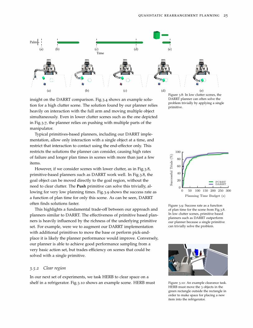
(a) (b) (c) (d) (e)Figure 3.8: In low clutter scenes, theDARRT planner can often solve theproblem trivially by applying a singleprimitive.
insight on the DARRT comparison. Fig.3.4 shows an example solu-tion for a high clutter scene. The solution found by our planner reliesheavily on interaction with the full arm and moving multiple objectsimultaneously. Even in lower clutter scenes such as the one depictedin Fig.3.7, the planner relies on pushing with multiple parts of themanipulator.
Typical primitives-based planners, including our DARRT imple-mentation, allow only interaction with a single object at a time, andrestrict that interaction to contact using the end-effector only. Thisrestricts the solutions the planner can consider, causing high ratesof failure and longer plan times in scenes with more than just a fewitems.
However, if we consider scenes with lower clutter, as in Fig.3.8,primitive-based planners such as DARRT work well. In Fig.3.8, thegoal object can be moved directly to the goal region, without theneed to clear clutter. The Push primitive can solve this trivially, al-lowing for very low planning times. Fig.3.9 shows the success rate asa function of plan time for only this scene. As can be seen, DARRToften finds solutions faster.
0 50 100 150 200 250 300
Planning Time Budget (s)
0
20
40
60
80
100
SuccessfulTrials
(%)
PCRRTDARRT
Figure 3.9: Success rate as a functionof plan time for the scene from Fig.3.8.In low clutter scenes, primitive basedplanners such as DARRT outperformour planner because a single primitivecan trivially solve the problem.
This highlights a fundamental trade-off between our approach andplanners similar to DARRT. The effectiveness of primitive based plan-ners is heavily influenced by the richness of the underlying primitiveset. For example, were we to augment our DARRT implementationwith additional primitives to move the base or perform pick-and-place it is likely the planner performance would improve. Conversely,our planner is able to achieve good performance sampling from avery basic action set, but trades efficiency on scenes that could besolved with a single primitive.
3.5.2 Clear region
Figure 3.10: An example clearance task.HERB must move the 3 objects in thegreen rectangle outside the rectangle inorder to make space for placing a newitem into the refrigerator.
In our next set of experiments, we task HERB to clear space on ashelf in a refrigerator. Fig.3.10 shows an example scene. HERB must
26 robust rearrangement planning using nonprehensile interaction
Finger1
Wrist
Finger2
Palm
(a) (b) (c) (d) (e)Time
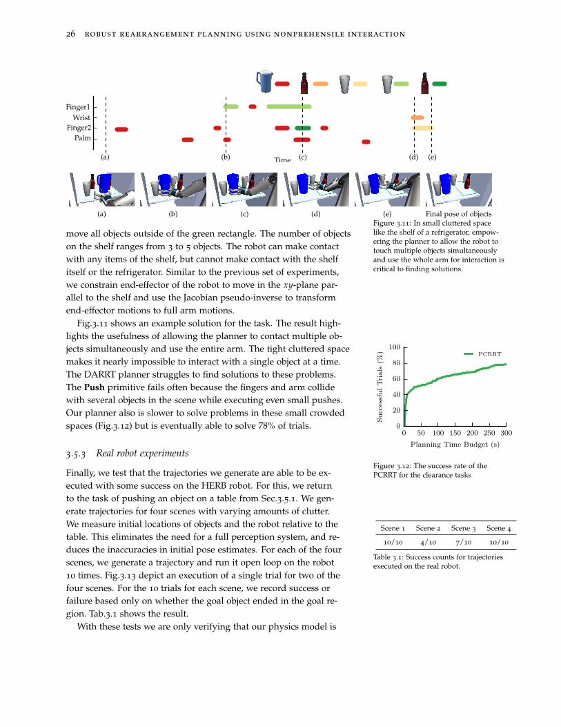
(a) (b) (c) (d) (e) Final pose of objectsFigure 3.11: In small cluttered spacelike the shelf of a refrigerator, empow-ering the planner to allow the robot totouch multiple objects simultaneouslyand use the whole arm for interaction iscritical to finding solutions.
move all objects outside of the green rectangle. The number of objectson the shelf ranges from 3 to 5 objects. The robot can make contactwith any items of the shelf, but cannot make contact with the shelfitself or the refrigerator. Similar to the previous set of experiments,we constrain end-effector of the robot to move in the xy-plane par-allel to the shelf and use the Jacobian pseudo-inverse to transformend-effector motions to full arm motions.
Fig.3.11 shows an example solution for the task. The result high-lights the usefulness of allowing the planner to contact multiple ob-jects simultaneously and use the entire arm. The tight cluttered spacemakes it nearly impossible to interact with a single object at a time.The DARRT planner struggles to find solutions to these problems.The Push primitive fails often because the fingers and arm collidewith several objects in the scene while executing even small pushes.Our planner also is slower to solve problems in these small crowdedspaces (Fig.3.12) but is eventually able to solve 78% of trials.
0 50 100 150 200 250 300
Planning Time Budget (s)
0
20
40
60
80
100
SuccessfulTrials
(%) PCRRT
Figure 3.12: The success rate of thePCRRT for the clearance tasks
3.5.3 Real robot experiments
Scene 1 Scene 2 Scene 3 Scene 4
10/10 4/10 7/10 10/10
Table 3.1: Success counts for trajectoriesexecuted on the real robot.
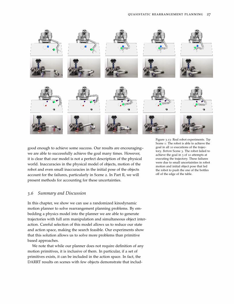
Finally, we test that the trajectories we generate are able to be ex-ecuted with some success on the HERB robot. For this, we returnto the task of pushing an object on a table from Sec.3.5.1. We gen-erate trajectories for four scenes with varying amounts of clutter.We measure initial locations of objects and the robot relative to thetable. This eliminates the need for a full perception system, and re-duces the inaccuracies in initial pose estimates. For each of the fourscenes, we generate a trajectory and run it open loop on the robot10 times. Fig.3.13 depict an execution of a single trial for two of thefour scenes. For the 10 trials for each scene, we record success orfailure based only on whether the goal object ended in the goal re-gion. Tab.3.1 shows the result.
With these tests we are only verifying that our physics model is
quasistatic rearrangement planning 27
Figure 3.13: Real robot experiments. TopScene 1: The robot is able to achieve thegoal in all 10 executions of the trajec-tory. Bottom Scene 3. The robot failed toachieve the goal in 3 of 10 attempts atexecuting the trajectory. These failureswere due to small uncertainties in robotmotion and initial object pose that ledthe robot to push the one of the bottlesoff of the edge of the table.
good enough to achieve some success. Our results are encouraging–we are able to successfully achieve the goal many times. However,it is clear that our model is not a perfect description of the physicalworld. Inaccuracies in the physical model of objects, motion of therobot and even small inaccuracies in the initial pose of the objectsaccount for the failures, particularly in Scene 2. In Part II, we willpresent methods for accounting for these uncertainties.
3.6 Summary and Discussion
In this chapter, we show we can use a randomized kinodynamicmotion planner to solve rearrangement planning problems. By em-bedding a physics model into the planner we are able to generatetrajectories with full arm manipulation and simultaneous object inter-action. Careful selection of this model allows us to reduce our stateand action space, making the search feasible. Our experiments showthat this solution allows us to solve more problems than primitivebased approaches.
We note that while our planner does not require definition of anymotion primitives, it is inclusive of them. In particular, if a set ofprimitives exists, it can be included in the action space. In fact, theDARRT results on scenes with few objects demonstrate that includ-

28 robust rearrangement planning using nonprehensile interaction
ing such primitives may in fact be very beneficial to overall planningtime. In the next chapter, we explore this idea in more detail. Addi-tionally, our planner can itself be used as a primitive in a hierarchicalplanner such as [16, 31]. While this thesis does not explore this ideain detail, we do provide some initial thoughts and further discussionin Ch.11.
4
Improving Randomized Rearrangement Planning
In this chapter, we present methods to improve upon the basic im-plementation described in Ch.3. In particular we focus on improvingthe speed and efficiency in generating solutions in Sec.4.2 and Sec.4.3and improving the quality of the final result in Sec.4.4.
4.1 Timing Analysis
0 10 20 30 40 50 60 70
Percent of Total Time (%)
Near.Neigh.
Lookup
GoalSample
Dist.Metric
RandomSample
TreeExt.
Figure 4.1: A breakdown of the timespent by the planner.
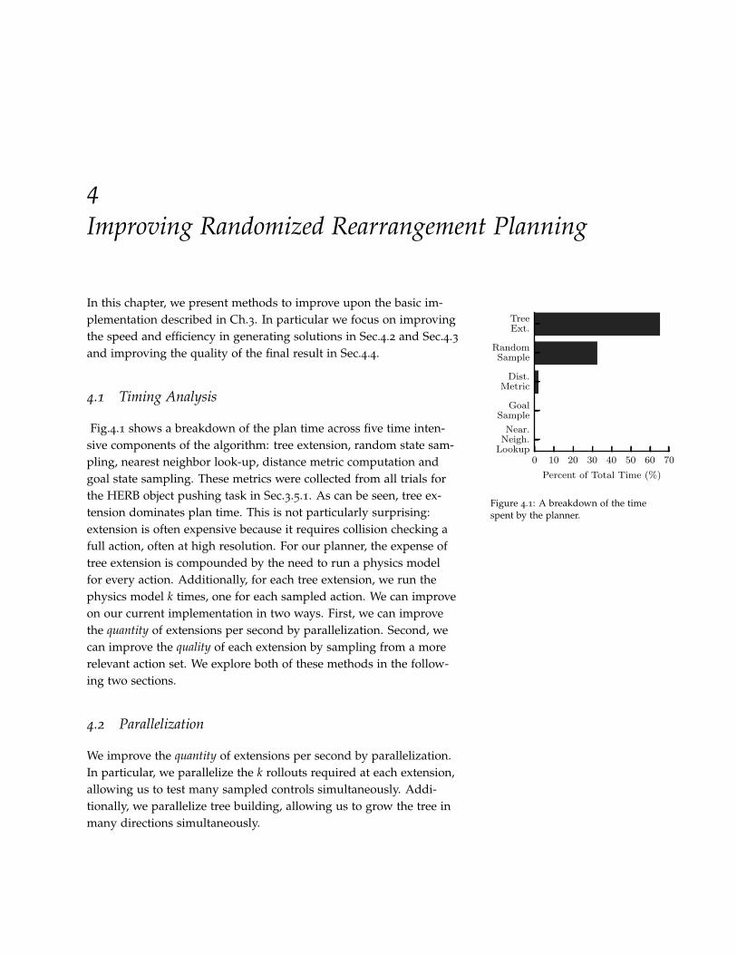
Fig.4.1 shows a breakdown of the plan time across five time inten-sive components of the algorithm: tree extension, random state sam-pling, nearest neighbor look-up, distance metric computation andgoal state sampling. These metrics were collected from all trials forthe HERB object pushing task in Sec.3.5.1. As can be seen, tree ex-tension dominates plan time. This is not particularly surprising:extension is often expensive because it requires collision checking afull action, often at high resolution. For our planner, the expense oftree extension is compounded by the need to run a physics modelfor every action. Additionally, for each tree extension, we run thephysics model k times, one for each sampled action. We can improveon our current implementation in two ways. First, we can improvethe quantity of extensions per second by parallelization. Second, wecan improve the quality of each extension by sampling from a morerelevant action set. We explore both of these methods in the follow-ing two sections.
4.2 Parallelization
We improve the quantity of extensions per second by parallelization.In particular, we parallelize the k rollouts required at each extension,allowing us to test many sampled controls simultaneously. Addi-tionally, we parallelize tree building, allowing us to grow the tree inmany directions simultaneously.
30 robust rearrangement planning using nonprehensile interaction
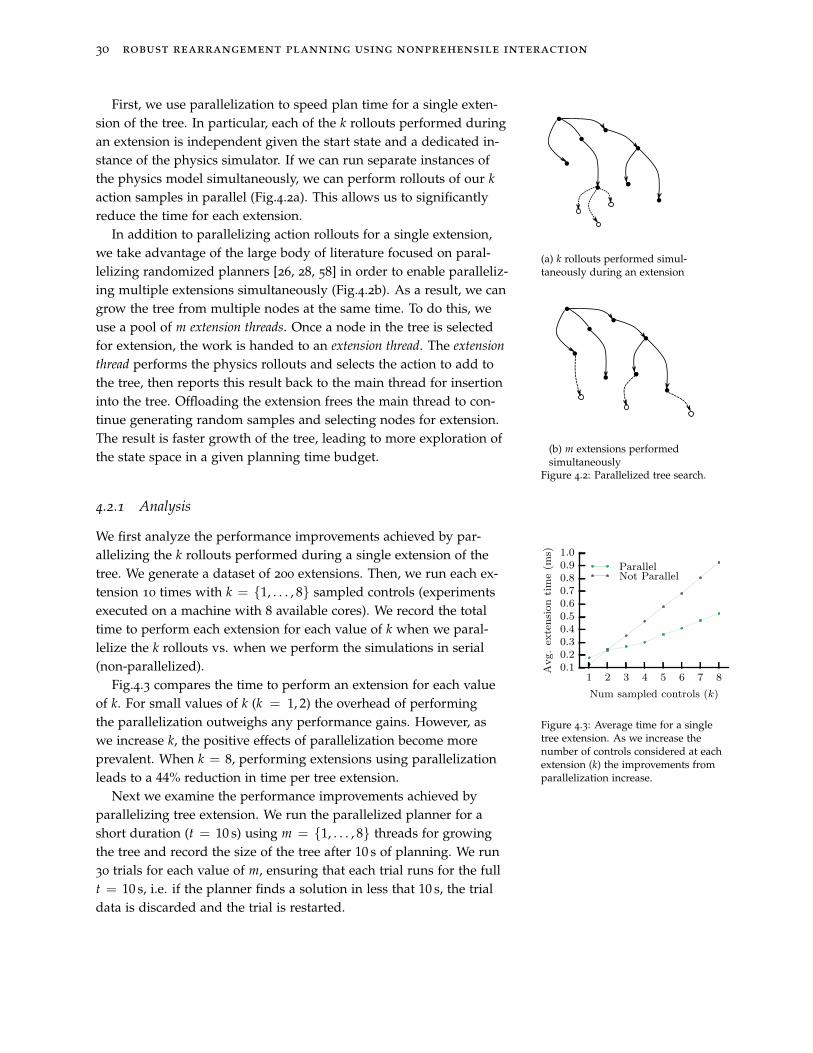
First, we use parallelization to speed plan time for a single exten-sion of the tree. In particular, each of the k rollouts performed duringan extension is independent given the start state and a dedicated in-stance of the physics simulator. If we can run separate instances ofthe physics model simultaneously, we can perform rollouts of our k
action samples in parallel (Fig.4.2a). This allows us to significantlyreduce the time for each extension.
(a) k rollouts performed simul-taneously during an extension
(b) m extensions performedsimultaneously
Figure 4.2: Parallelized tree search.
In addition to parallelizing action rollouts for a single extension,we take advantage of the large body of literature focused on paral-lelizing randomized planners [26, 28, 58] in order to enable paralleliz-ing multiple extensions simultaneously (Fig.4.2b). As a result, we cangrow the tree from multiple nodes at the same time. To do this, weuse a pool of m extension threads. Once a node in the tree is selectedfor extension, the work is handed to an extension thread. The extension
thread performs the physics rollouts and selects the action to add tothe tree, then reports this result back to the main thread for insertioninto the tree. Offloading the extension frees the main thread to con-tinue generating random samples and selecting nodes for extension.The result is faster growth of the tree, leading to more exploration ofthe state space in a given planning time budget.
4.2.1 Analysis
We first analyze the performance improvements achieved by par-allelizing the k rollouts performed during a single extension of thetree. We generate a dataset of 200 extensions. Then, we run each ex-tension 10 times with k = {1, . . . , 8} sampled controls (experimentsexecuted on a machine with 8 available cores). We record the totaltime to perform each extension for each value of k when we paral-lelize the k rollouts vs. when we perform the simulations in serial(non-parallelized).
1 2 3 4 5 6 7 8
Num sampled controls (k)
0.10.20.30.40.50.60.70.80.91.0
Avg.ex
tensiontime(m
s)
ParallelNot Parallel
Figure 4.3: Average time for a singletree extension. As we increase thenumber of controls considered at eachextension (k) the improvements fromparallelization increase.
Fig.4.3 compares the time to perform an extension for each valueof k. For small values of k (k = 1, 2) the overhead of performingthe parallelization outweighs any performance gains. However, aswe increase k, the positive effects of parallelization become moreprevalent. When k = 8, performing extensions using parallelizationleads to a 44% reduction in time per tree extension.
Next we examine the performance improvements achieved byparallelizing tree extension. We run the parallelized planner for ashort duration (t = 10 s) using m = {1, . . . , 8} threads for growingthe tree and record the size of the tree after 10 s of planning. We run30 trials for each value of m, ensuring that each trial runs for the fullt = 10 s, i.e. if the planner finds a solution in less that 10 s, the trialdata is discarded and the trial is restarted.

improving randomized rearrangement planning 31
Fig.4.4 shows the average tree size across all trials. For m =
{1, . . . , 5} we see significantly improved tree size by increasing thenumber of threads simultaneously extending the tree. However, form > 5 the performance improvements disappear. At this point, thebottleneck becomes random sample generation, i.e. the main threadcannot select nodes for extension fast enough to keep all workerthreads running.
1 2 3 4 5 6 7 8
Num tree threads (m)
Avg.TreeSize
Figure 4.4: Average tree size after 10 sof tree growth. Increasing the availablethreads for simultaneous tree growthm increases the number of extensionswe can consider, growing the tree largerfaster.
0 50 100 150 200 250 300
Planning Time Budget (s)
0
20
40
60
80
100
Successfu
lTrials
(%)
ExtensionsTree growthBaseline
Figure 4.5: Average plan time acrosssuccessful trials
Finally, we test the affect of each of these two methods on the fulltest dataset for the HERB pushing task from Sec.3.5.1. We test thedefault planner that did not use any parallelization (Baseline) againsta planner that parallelizes rollouts during extension (Extensions,k = 8) and a planner that parallelizes tree growth (Tree growth,m = 5). Fig.4.5 shows the results. Parallelizing extensions doesnot demonstrate a significant improvement however it also does notdemonstrate decreased performance, despite the fact that we rollout5 more samples per extension compared to results from Sec.3.5.1.Parallelizing tree building does lead to significantly higher overallsuccess because we explore the state space faster.
4.3 Object-centric Action Spaces
This section is adapted from King etal. [63].
In this section, we improve the quality of each extension by biasingour control sampling to regions of control space likely to create ex-tensions toward our sampled state. This will lead to the need forfewer overall extensions, reducing plan time.
The planner presented in Ch.3 samples lower-level primitives thatdescribe only robot motions during tree extension. These primitiveshave no object-relevant intent or explicit object interaction. The useof these robot-centric motions contrasts methods from previous worksthat have solved rearrangement planning using high-level primitivesthat describe purely object-centric actions [15, 36, 113, 116, 119]. Inthese works, the object-centric actions guide the planners to performspecific actions on specific objects. Such actions can be highly ef-fective – allowing the planner to make large advancements towardsthe goal. However, the use of only these actions limits the types ofsolutions generated by the planner. In particular, these interactionsusually involve only contact with a single part of the robot, i.e. theend-effector, and often forbid simultaneous object contact.
The use of robot-centric motions in our planner relaxes the restric-tions imposed by using object-centric actions, allowing the planner togenerate solutions that exhibit whole arm interaction and simultane-ous object contact. However, the planner suffers from long plan timesdue to the lack of goal directed motions available to the planner.
Our insight is that both types of actions are critical to generating
32 robust rearrangement planning using nonprehensile interaction
expressive solutions quickly. By integrating the two action types, wecan use the freedom of interaction fundamental to the robot-centric
actions while still allowing for the goal oriented growth central to theobject-centric methods. In this section, we first provide an overviewof object-centric based methods, then describe a modification to ourplanner that allows for incorporating such actions.
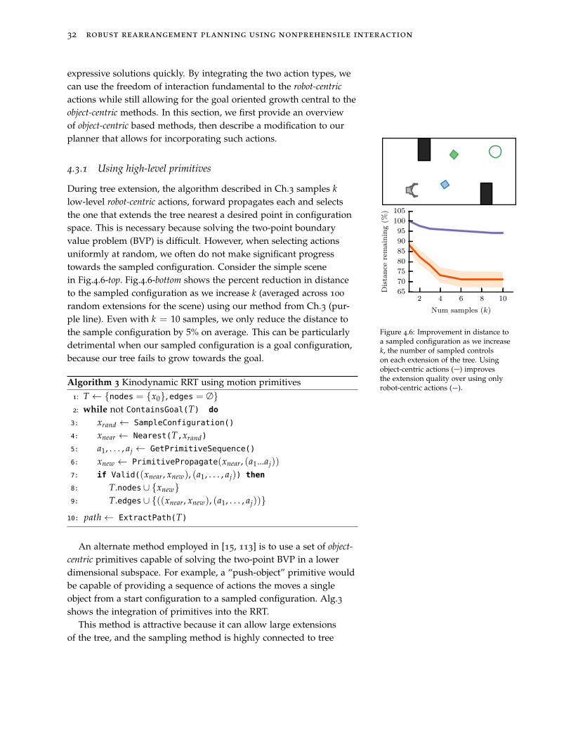
4.3.1 Using high-level primitives
2 4 6 8 10
Num samples (k)
65
70
75
80
85
90
95
100
105
Distance
remaining(%
)
Figure 4.6: Improvement in distance toa sampled configuration as we increasek, the number of sampled controlson each extension of the tree. Usingobject-centric actions ( ) improvesthe extension quality over using onlyrobot-centric actions ( ).
During tree extension, the algorithm described in Ch.3 samples k
low-level robot-centric actions, forward propagates each and selectsthe one that extends the tree nearest a desired point in configurationspace. This is necessary because solving the two-point boundaryvalue problem (BVP) is difficult. However, when selecting actionsuniformly at random, we often do not make significant progresstowards the sampled configuration. Consider the simple scenein Fig.4.6-top. Fig.4.6-bottom shows the percent reduction in distanceto the sampled configuration as we increase k (averaged across 100
random extensions for the scene) using our method from Ch.3 (pur-ple line). Even with k = 10 samples, we only reduce the distance tothe sample configuration by 5% on average. This can be particularlydetrimental when our sampled configuration is a goal configuration,because our tree fails to grow towards the goal.
Algorithm 3 Kinodynamic RRT using motion primitives
1: T ← {nodes = {x0}, edges = ∅}
2: while not ContainsGoal(T) do
3: xrand ← SampleConfiguration()
4: xnear ← Nearest(T,xrand)
5: a1, . . . , aj ← GetPrimitiveSequence()
6: xnew ← PrimitivePropagate(xnear, (a1...aj))
7: if Valid((xnear, xnew), (a1, . . . , aj)) then
8: T.nodes∪ {xnew}
9: T.edges∪ {((xnear, xnew), (a1, . . . , aj))}
10: path← ExtractPath(T)
An alternate method employed in [15, 113] is to use a set of object-
centric primitives capable of solving the two-point BVP in a lowerdimensional subspace. For example, a “push-object” primitive wouldbe capable of providing a sequence of actions the moves a singleobject from a start configuration to a sampled configuration. Alg.3shows the integration of primitives into the RRT.
This method is attractive because it can allow large extensionsof the tree, and the sampling method is highly connected to tree
improving randomized rearrangement planning 33
growth. Fig.4.6-bottom (orange) shows the reduction in distance tothe sampled state on an extension is much better when using theseobject-centric primitives. This is particularly useful when the sample isa goal state: it allows the tree to grow to the goal.
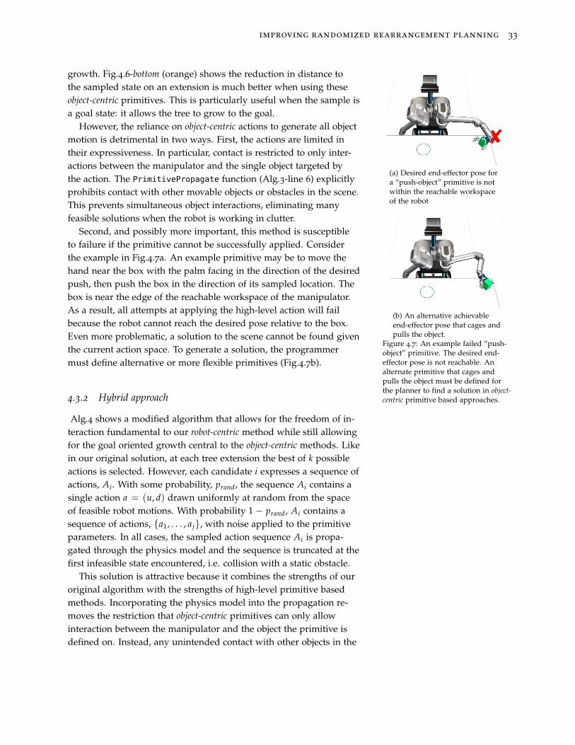
However, the reliance on object-centric actions to generate all objectmotion is detrimental in two ways. First, the actions are limited intheir expressiveness. In particular, contact is restricted to only inter-actions between the manipulator and the single object targeted bythe action. The PrimitivePropagate function (Alg.3-line 6) explicitlyprohibits contact with other movable objects or obstacles in the scene.This prevents simultaneous object interactions, eliminating manyfeasible solutions when the robot is working in clutter.
(a) Desired end-effector pose fora “push-object” primitive is notwithin the reachable workspaceof the robot
(b) An alternative achievableend-effector pose that cages andpulls the object.
Figure 4.7: An example failed “push-object” primitive. The desired end-effector pose is not reachable. Analternate primitive that cages andpulls the object must be defined forthe planner to find a solution in object-centric primitive based approaches.
Second, and possibly more important, this method is susceptibleto failure if the primitive cannot be successfully applied. Considerthe example in Fig.4.7a. An example primitive may be to move thehand near the box with the palm facing in the direction of the desiredpush, then push the box in the direction of its sampled location. Thebox is near the edge of the reachable workspace of the manipulator.As a result, all attempts at applying the high-level action will failbecause the robot cannot reach the desired pose relative to the box.Even more problematic, a solution to the scene cannot be found giventhe current action space. To generate a solution, the programmermust define alternative or more flexible primitives (Fig.4.7b).
4.3.2 Hybrid approach
Alg.4 shows a modified algorithm that allows for the freedom of in-teraction fundamental to our robot-centric method while still allowingfor the goal oriented growth central to the object-centric methods. Likein our original solution, at each tree extension the best of k possibleactions is selected. However, each candidate i expresses a sequence ofactions, Ai. With some probability, prand, the sequence Ai contains asingle action a = (u, d) drawn uniformly at random from the spaceof feasible robot motions. With probability 1− prand, Ai contains asequence of actions, {a1, . . . , aj}, with noise applied to the primitiveparameters. In all cases, the sampled action sequence Ai is propa-gated through the physics model and the sequence is truncated at thefirst infeasible state encountered, i.e. collision with a static obstacle.
This solution is attractive because it combines the strengths of ouroriginal algorithm with the strengths of high-level primitive basedmethods. Incorporating the physics model into the propagation re-moves the restriction that object-centric primitives can only allowinteraction between the manipulator and the object the primitive isdefined on. Instead, any unintended contact with other objects in the
34 robust rearrangement planning using nonprehensile interaction
Algorithm 4 Kinodynamic RRT using hybrid action sampling
1: T ← {nodes = {x0}, edges = ∅}
2: while not ContainsGoal(T) do
3: xrand ← SampleConfiguration()
4: xnear ← Nearest(T,xrand)
5: for i = 1 . . . k do
6: r ← Uniform01()
7: if r < prand then
8: Ai ← SampleUniformAction()
9: else
10: Ai ← SamplePrimitiveSequence()
11: (xi, Ai)← PhysicsPropagate(xnear, Ai)
12: i∗ = argmini Dist(xi, xrand)
13: if Valid((xnear, xi∗), Ai∗)) then
14: T.nodes∪ {xi∗}
15: T.edges∪ {((xnear, xi∗), Ai∗)}
16: path← ExtractPath(T)
scene can be modeled. Often, this unintended contact is not detri-mental to overall goal achievement and should be allowed. Samplingrandom actions with some probability allows the planner to generateactions that move an object when all primitives targeted at the objectwould fail (i.e. the example in Fig.4.7).
4.3.3 Experiments and Results
Again, we implement the planner described in this section in theOMPL framework. We test three versions of our updated planner.First, we set prand = 0. This forces the planner to always sampleobject-centric actions. We denote this planner object-centric in all re-sults. Second, we set prand = 1. This forces the planner to alwayssample robot-centric actions. We note this is exactly the planner origi-nally presented in Ch.3. We denote these results robot-centric in thissection. Finally, we set prand = 0.5. This allows the planner to chooseobject-centric or robot-centric actions with equal probability. We denotethis planner as hybrid in all results. In the next section, we discussalternate values for prand and their impact on the results.
Using the planner, we execute a set of experiments to test thefollowing hypotheses:
H.1 Propagating object-centric primitives through the physicsmodel during tree extension improves the performance of plannersthat purely rely on these primitives by allowing the primitives to
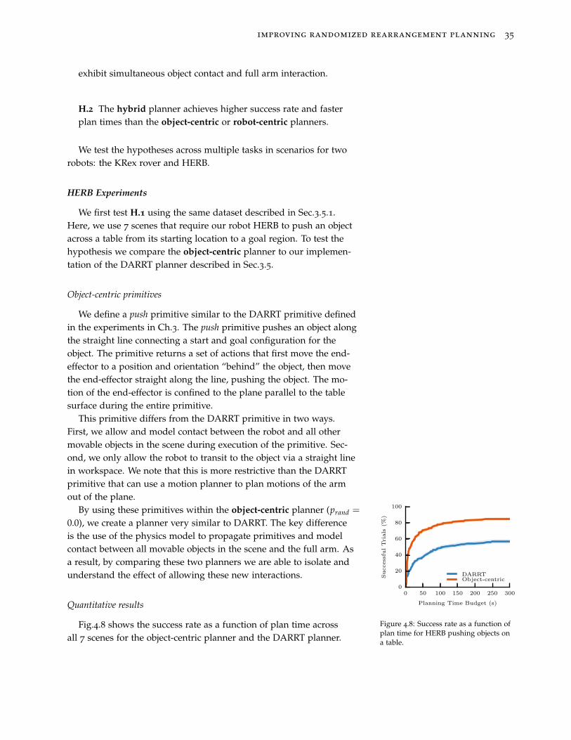
improving randomized rearrangement planning 35
exhibit simultaneous object contact and full arm interaction.
H.2 The hybrid planner achieves higher success rate and fasterplan times than the object-centric or robot-centric planners.
We test the hypotheses across multiple tasks in scenarios for tworobots: the KRex rover and HERB.
HERB Experiments
We first test H.1 using the same dataset described in Sec.3.5.1.Here, we use 7 scenes that require our robot HERB to push an objectacross a table from its starting location to a goal region. To test thehypothesis we compare the object-centric planner to our implemen-tation of the DARRT planner described in Sec.3.5.
Object-centric primitives
We define a push primitive similar to the DARRT primitive definedin the experiments in Ch.3. The push primitive pushes an object alongthe straight line connecting a start and goal configuration for theobject. The primitive returns a set of actions that first move the end-effector to a position and orientation “behind” the object, then movethe end-effector straight along the line, pushing the object. The mo-tion of the end-effector is confined to the plane parallel to the tablesurface during the entire primitive.
This primitive differs from the DARRT primitive in two ways.First, we allow and model contact between the robot and all othermovable objects in the scene during execution of the primitive. Sec-ond, we only allow the robot to transit to the object via a straight linein workspace. We note that this is more restrictive than the DARRTprimitive that can use a motion planner to plan motions of the armout of the plane.
By using these primitives within the object-centric planner (prand =
0.0), we create a planner very similar to DARRT. The key differenceis the use of the physics model to propagate primitives and modelcontact between all movable objects in the scene and the full arm. Asa result, by comparing these two planners we are able to isolate andunderstand the effect of allowing these new interactions.
0 50 100 150 200 250 300
Planning Time Budget (s)
0
20
40
60
80
100
Successfu
lTrials
(%)
DARRTObject-centric
Figure 4.8: Success rate as a function ofplan time for HERB pushing objects ona table.
Quantitative results
Fig.4.8 shows the success rate as a function of plan time acrossall 7 scenes for the object-centric planner and the DARRT planner.
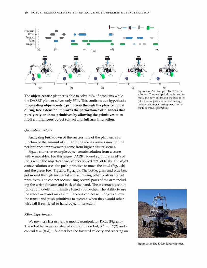
36 robust rearrangement planning using nonprehensile interaction
ForearmWrist
Finger1
Finger2Palm
Time(a) (b) (c) (d) (e)
(a) (b) (c) (d) (e)Figure 4.9: An example object-centricsolution. The push primitive is used tomove the bowl in (b) and the box in (c)-(e). Other objects are moved throughincidental contact during execution ofpush or transit primitives.
The object-centric planner is able to solve 84% of problems whilethe DARRT planner solves only 57%. This confirms our hypothesis:Propagating object-centric primitives through the physics model
during tree extension improves the performance of planners that
purely rely on these primitives by allowing the primitives to ex-
hibit simultaneous object contact and full arm interaction.
Qualitative analysis
Analyzing breakdown of the success rate of the planners as afunction of the amount of clutter in the scenes reveals much of theperformance improvements come from higher clutter scenes.
Fig.4.9 shows an example object-centric solution from a scenewith 6 movables. For this scene, DARRT found solutions in 24% oftrials while the object-centric planner solved 98% of trials. The object-
centric solution uses the push primitive to move the bowl (Fig.4.9b)and the green box (Fig.4.9c, Fig.4.9d). The bottle, glass and blue boxget moved through incidental contact during other push or transitprimitives. The contact occurs using several parts of the arm includ-ing the wrist, forearm and back of the hand. These contacts are nottypically modeled in primitive based approaches. The ability to usethe whole arm and make simultaneous contact with objects allowsthe transit and push primitives to succeed when they would other-wise fail if restricted to hand-object interaction.
KRex Experiments
Figure 4.10: The K-Rex lunar explorer.
We next test H.2 using the mobile manipulator KRex (Fig.4.10).The robot behaves as a steered car. For this robot, XR = SE(2) and acontrol u = (v, δ) ∈ U describes the forward velocity and steering an-
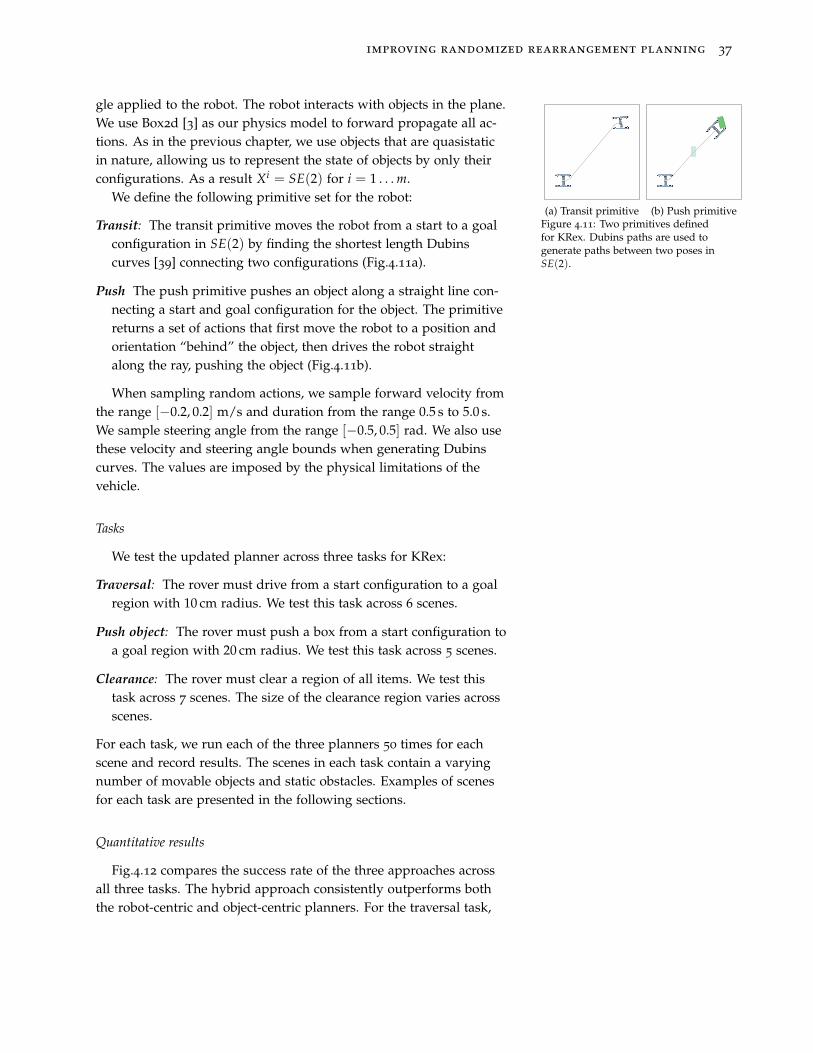
improving randomized rearrangement planning 37
gle applied to the robot. The robot interacts with objects in the plane.We use Box2d [3] as our physics model to forward propagate all ac-tions. As in the previous chapter, we use objects that are quasistaticin nature, allowing us to represent the state of objects by only theirconfigurations. As a result Xi = SE(2) for i = 1 . . . m.
(a) Transit primitive (b) Push primitiveFigure 4.11: Two primitives definedfor KRex. Dubins paths are used togenerate paths between two poses inSE(2).
We define the following primitive set for the robot:
Transit: The transit primitive moves the robot from a start to a goalconfiguration in SE(2) by finding the shortest length Dubinscurves [39] connecting two configurations (Fig.4.11a).
Push The push primitive pushes an object along a straight line con-necting a start and goal configuration for the object. The primitivereturns a set of actions that first move the robot to a position andorientation “behind” the object, then drives the robot straightalong the ray, pushing the object (Fig.4.11b).
When sampling random actions, we sample forward velocity fromthe range [−0.2, 0.2] m/s and duration from the range 0.5 s to 5.0 s.We sample steering angle from the range [−0.5, 0.5] rad. We also usethese velocity and steering angle bounds when generating Dubinscurves. The values are imposed by the physical limitations of thevehicle.
Tasks
We test the updated planner across three tasks for KRex:
Traversal: The rover must drive from a start configuration to a goalregion with 10 cm radius. We test this task across 6 scenes.
Push object: The rover must push a box from a start configuration toa goal region with 20 cm radius. We test this task across 5 scenes.
Clearance: The rover must clear a region of all items. We test thistask across 7 scenes. The size of the clearance region varies acrossscenes.
For each task, we run each of the three planners 50 times for eachscene and record results. The scenes in each task contain a varyingnumber of movable objects and static obstacles. Examples of scenesfor each task are presented in the following sections.
Quantitative results
Fig.4.12 compares the success rate of the three approaches acrossall three tasks. The hybrid approach consistently outperforms boththe robot-centric and object-centric planners. For the traversal task,

38 robust rearrangement planning using nonprehensile interaction
0 10 20 30 40 50 60
Planning Time Budget (s)
0
20
40
60
80
100
Successfu
lTrials
(%)
(a) Traversal
0 10 20 30 40 50 60
Planning Time Budget (s)
0
20
40
60
80
100
Successfu
lTrials
(%)
(b) Push object
0 10 20 30 40 50 60
Planning Time Budget (s)
0
20
40
60
80
100
Successfu
lTrials
(%)
(c) Clearance
Figure 4.12: The success rate as afunction of plan time for each of thethree KRex tasks. The hybrid planner( ) outperforms both the object-centric( and robot-centric ( ) plannersacross all tasks.
the hybrid approach is able to solve 99% of trials, outperformingboth the object-centric (65%) and robot-centric (60%) methods. Inaddition, it finds solutions much faster, solving over 75% of problemsin less than 10 s. Statistical analysis reveals a significant main effectfor plan time (F(2, 897) = 121.2, p < 0.0001) and success (F(2, 897) =84.61, p < 0.0001).
Similar results are revealed with statistical analysis of the pushobject task (plan time - F(2, 747) = 75.4(p < 0.0001), success rate -F(2, 747) = 49.32(p < 0.0001)) and the clearance task (plan time -F(2, 946) = 49.86(p < 0.00001), success rate F(2, 946) = 39.17(p <
0.00001)).Tukey HSD post-hoc analysis shows the hybrid approach differs
significantly from the robot-centric and object-centric approaches insuccess rate (p < 0.0001) and plan time (p < 0.0001) on all threetasks.
This analysis supports our H.2: The hybrid planner achieves
higher success rate and faster plan times that the object-centric or
robot-centric planners.
Qualitative analysis
While we have shown that in general the hybrid planner solvesproblems more effectively than using only robot-centric or object-centric actions, a deeper look at solutions to individual scenes pro-vides further insight into these gains.
(a) Traversal (b) Push object (c) Clearance
Figure 4.13: A robot-centric ( ) andobject-centric ( ) solution easy scenesfor each task. Left: The robot musttraverse through an empty environmentto a goal region in the top right corner.Middle: The robot must push the bluebox into a goal region in the top rightcorner. All green boxes are movableobjects. Right The robot must push thegreen box from its start pose in themiddle of the environment to any poseoutside the region outlined in green.
Fig.4.13 depicts a pure robot-centric and pure object-centric solu-tion for a single scene for each of the three tasks. These scenes are all
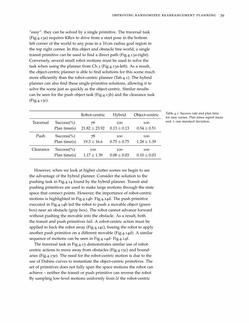
improving randomized rearrangement planning 39
“easy”: they can be solved by a single primitive. The traversal task(Fig.4.13a) requires KRex to drive from a start pose in the bottomleft corner of the world to any pose in a 10 cm radius goal region inthe top right corner. In this object and obstacle free world, a singletransit primitive can be used to find a direct path (Fig.4.13a-right).Conversely, several small robot motions must be used to solve thetask when using the planner from Ch.3 (Fig.4.13a-left). As a result,the object-centric planner is able to find solutions for this scene muchmore efficiently than the robot-centric planner (Tab.4.1). The hybridplanner can also find these single-primitive solutions, allowing it tosolve the scene just as quickly as the object-centric. Similar resultscan be seen for the push object task (Fig.4.13b) and the clearance task(Fig.4.13c).
Robot-centric Hybrid Object-centric
Traversal Success(%) 76 100 100
Plan time(s) 21.82± 23.92 0.13± 0.13 0.54± 0.51
Push Success(%) 78 100 100
Plan time(s) 19.3± 16.6 0.75± 0.75 1.28± 1.39
Clearance Success(%) 100 100 100
Plan time(s) 1.17± 1.39 0.08± 0.03 0.10± 0.03
Table 4.1: Success rate and plan timefor easy scenes. Plan times report meanand ± one standard deviation.
However, when we look at higher clutter scenes we begin to seethe advantage of the hybrid planner. Consider the solution to thepushing task in Fig.4.14 found by the hybrid planner. Transit andpushing primitives are used to make large motions through the statespace that connect points. However, the importance of robot-centricmotions is highlighted in Fig.4.14b- Fig.4.14d. The push primitiveexecuted in Fig.4.14b led the robot to push a movable object (greenbox) near an obstacle (gray box). The robot cannot advance forwardwithout pushing the movable into the obstacle. As a result, boththe transit and push primitives fail. A robot-centric action must beapplied to back the robot away (Fig.4.14c), freeing the robot to applyanother push primitive on a different movable (Fig.4.14d). A similarsequence of motions can be seen in Fig.4.14d- Fig.4.14f.
The traversal task in Fig.4.15 demonstrates similar use of robot-centric actions to move away from obstacles (Fig.4.15c) and bound-aries (Fig.4.15e). The need for the robot-centric motion is due to theuse of Dubins curves to instantiate the object-centric primitives. Theset of primitives does not fully span the space motions the robot canachieve – neither the transit or push primitive can reverse the robot.By sampling low-level motions uniformly from U the robot-centric
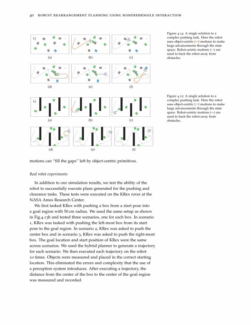
40 robust rearrangement planning using nonprehensile interaction
(a) (b) (c)
(d) (e) (f)
Figure 4.14: A single solution to acomplex pushing task. Here the robotuses object-centric ( ) motions to makelarge advancements through the statespace. Robot-centric motions ( ) areused to back the robot away fromobstacles.
(a) (b) (c)
(d) (e) (f)
Figure 4.15: A single solution to acomplex pushing task. Here the robotuses object-centric ( ) motions to makelarge advancements through the statespace. Robot-centric motions ( ) areused to back the robot away fromobstacles.
motions can “fill the gaps” left by object-centric primitives.
Real robot experiments
In addition to our simulation results, we test the ability of therobot to successfully execute plans generated for the pushing andclearance tasks. These tests were executed on the KRex rover at theNASA Ames Research Center.
We first tasked KRex with pushing a box from a start pose intoa goal region with 50 cm radius. We used the same setup as shownin Fig.4.13b and tested three scenarios, one for each box. In scenario1, KRex was tasked with pushing the left-most box from its startpose to the goal region. In scenario 2, KRex was asked to push thecenter box and in scenario 3, KRex was asked to push the right-mostbox. The goal location and start position of KRex were the sameacross scenarios. We used the hybrid planner to generate a trajectoryfor each scenario. We then executed each trajectory on the robot10 times. Objects were measured and placed in the correct startinglocation. This eliminated the errors and complexity that the use ofa perception system introduces. After executing a trajectory, thedistance from the center of the box to the center of the goal regionwas measured and recorded.
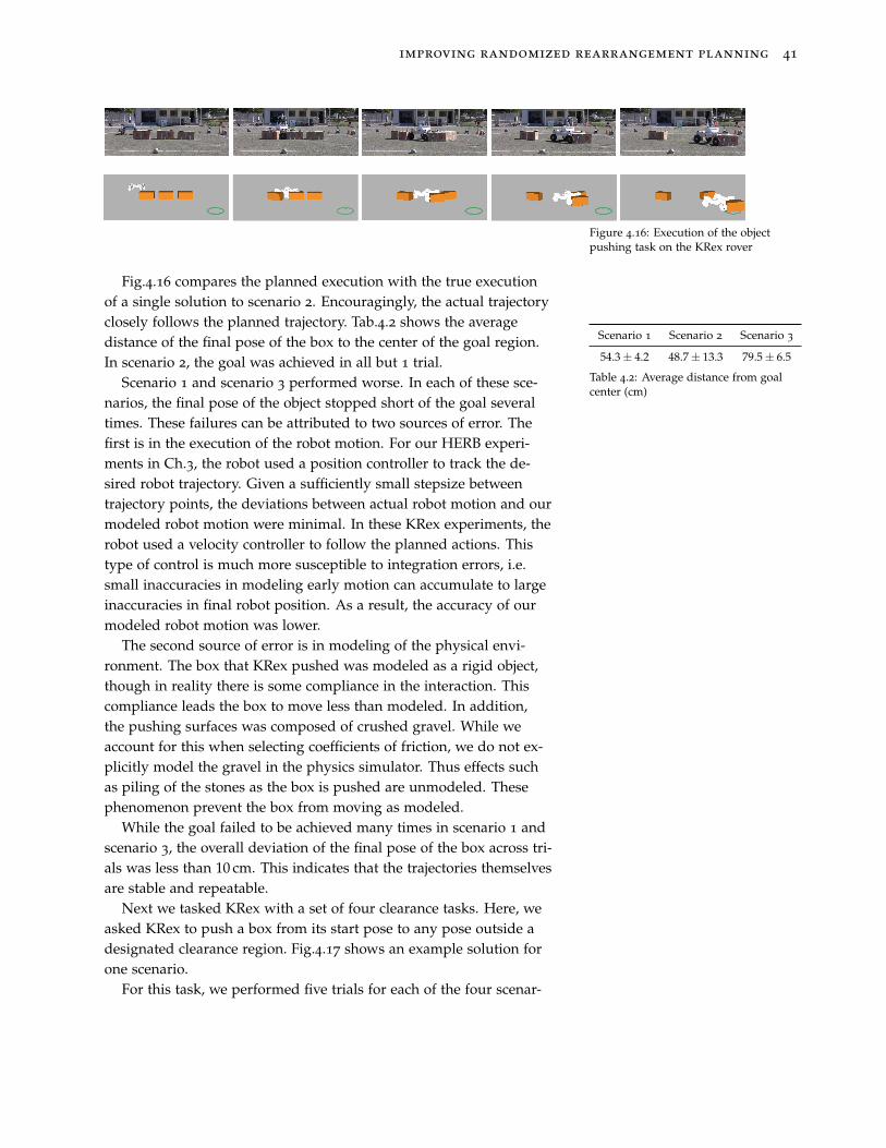
improving randomized rearrangement planning 41
Figure 4.16: Execution of the objectpushing task on the KRex rover
Fig.4.16 compares the planned execution with the true executionof a single solution to scenario 2. Encouragingly, the actual trajectoryclosely follows the planned trajectory. Tab.4.2 shows the averagedistance of the final pose of the box to the center of the goal region.In scenario 2, the goal was achieved in all but 1 trial.
Scenario 1 Scenario 2 Scenario 3
54.3± 4.2 48.7± 13.3 79.5± 6.5
Table 4.2: Average distance from goalcenter (cm)
Scenario 1 and scenario 3 performed worse. In each of these sce-narios, the final pose of the object stopped short of the goal severaltimes. These failures can be attributed to two sources of error. Thefirst is in the execution of the robot motion. For our HERB experi-ments in Ch.3, the robot used a position controller to track the de-sired robot trajectory. Given a sufficiently small stepsize betweentrajectory points, the deviations between actual robot motion and ourmodeled robot motion were minimal. In these KRex experiments, therobot used a velocity controller to follow the planned actions. Thistype of control is much more susceptible to integration errors, i.e.small inaccuracies in modeling early motion can accumulate to largeinaccuracies in final robot position. As a result, the accuracy of ourmodeled robot motion was lower.
The second source of error is in modeling of the physical envi-ronment. The box that KRex pushed was modeled as a rigid object,though in reality there is some compliance in the interaction. Thiscompliance leads the box to move less than modeled. In addition,the pushing surfaces was composed of crushed gravel. While weaccount for this when selecting coefficients of friction, we do not ex-plicitly model the gravel in the physics simulator. Thus effects suchas piling of the stones as the box is pushed are unmodeled. Thesephenomenon prevent the box from moving as modeled.
While the goal failed to be achieved many times in scenario 1 andscenario 3, the overall deviation of the final pose of the box across tri-als was less than 10 cm. This indicates that the trajectories themselvesare stable and repeatable.
Next we tasked KRex with a set of four clearance tasks. Here, weasked KRex to push a box from its start pose to any pose outside adesignated clearance region. Fig.4.17 shows an example solution forone scenario.
For this task, we performed five trials for each of the four scenar-
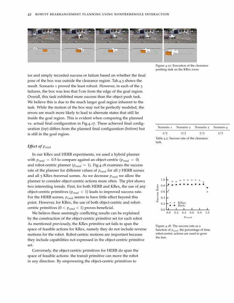
42 robust rearrangement planning using nonprehensile interaction
Figure 4.17: Execution of the clearancepushing task on the KRex rover
ios and simply recorded success or failure based on whether the finalpose of the box was outside the clearance region. Tab.4.3 shows theresult. Scenario 1 proved the least robust. However, in each of the 3
failures, the box was less that 5 cm from the edge of the goal region.Overall, this task exhibited more success than the object push task.We believe this is due to the much larger goal region inherent to thetask. While the motion of the box may not be perfectly modeled, theerrors are much more likely to lead to alternate states that still lieinside the goal region. This is evident when comparing the plannedvs. actual final configuration in Fig.4.17. These achieved final config-uration (top) differs from the planned final configuration (bottom) butis still in the goal region.
Scenario 1 Scenario 2 Scenario 3 Scenario 4
2/5 5/5 5/5 5/5
Table 4.3: Success rate of the clearancetask.
Effect of prand
In our KRex and HERB experiments, we used a hybrid plannerwith prand = 0.5 to compare against an object-centric (prand = 0)and robot-centric planner (prand = 1). Fig.4.18 examines the successrate of the planner for different values of prand for all 7 HERB scenesand all 5 KRex traversal scenes. As we decrease prand we allow theplanner to consider object-centric actions more often. The plot showstwo interesting trends. First, for both HERB and KRex, the use of anyobject-centric primitives (prand < 1) leads to improved success rate.For the HERB scenes, prand seems to have little effect beyond thispoint. However, for KRex, the use of both object-centric and robot-centric primitives (0 < prand < 1) proves beneficial.
0.0 0.2 0.4 0.6 0.8 1.0
prand
0.0
0.2
0.4
0.6
0.8
1.0
SuccessRate
KRexHerb
Figure 4.18: The success rate as afunction of prand, the percentage of timerobot-centric actions are used to growthe tree.
We believe these seemingly conflicting results can be explainedby the construction of the object-centric primitive set for each robot.As mentioned previously, the KRex primitive set fails to span thespace of feasible actions for KRex, namely they do not include reversemotions for the robot. Robot-centric motions are important becausethey include capabilities not expressed in the object-centric primitiveset.
Conversely, the object-centric primitives for HERB do span thespace of feasible actions: the transit primitive can move the robotin any direction. By empowering the object-centric primitives to
improving randomized rearrangement planning 43
(a) The initial path. (b) The two manipulator statesselected for connection.
(c) The new states generated forthe shortcut.
(d) The new states added after theshortcut.
Figure 4.19: The shortcutting algorithm.For simplicity, we depict only themotion of the end-effector. However,the whole arm is considered duringplanning. In (d) the motion of themanipulator and green object remainunchanged along the remainder of thepath. However, states are updated toreflect the new location of the blue boxand purple circle.
allow simultaneous object contact and full arm interaction, we haveimproved the strength and applicability of the primitive, renderingthe robot-centric actions less necessary for this task.
4.4 Path Shortcutting
Finally, in this section we improve the quality of the output of theplanners. The use of a randomized planner leads to paths that oftencontain unnecessary movements of the manipulator. Several post-processing techniques to smooth these paths have been introducedin the literature. One commonly used technique [43, 51, 108, 110] isto randomly select two points from the path and attempt to connectthem. If successful, intermediate points between the two selectedpoints are discarded from the path, and the new connection is added.
Use of this technique typically requires solving the two-pointboundary value problem to generate the new edge. As describedin Ch.3, this is non-trivial for our problem. Instead we employ aslightly altered technique illustrated in Fig.4.19.
Given a trajectory produced by our planner, we first randomlyselect two points in the trajectory (Fig.4.19b). We then attempt togenerate a new action to connect only the robot configuration inthese two states. If such an action is generated, we forward propagateit using our physics model, and record the new intermediate states(Fig.4.19c).
We note that the ending state of the shortcut action could differfrom the sampled state in the configuration of one or more movableobjects. For example, in Fig.4.19c the final state differs in the configu-ration of both the blue box and the purple circle. Because of this, wemust forward propagate all remaining actions in the trajectory andensure the goal is still achieved (Fig.4.19d). If successful, the updatedpath is accepted and the algorithm iterates.
4.4.1 Analysis
Original Shortcut
ManipulatorPath
Len
gth 9.0
5.8
Figure 4.20: Results from shortcuttingfor 15s.
To examine the performance of the shortcutting algorithm, we returnto the results provided in Sec.3.5.1. We run the shortcut algorithm
44 robust rearrangement planning using nonprehensile interaction
(a) Original scene (b) Manipulator path (c) Object pathFigure 4.21: An example shortcut. (b)The original path (dotted) containsunnecessary extra movements removedin the shortcut path (solid). This leadsto a new final pose of the robot andobject (filled) when compared to theoriginal (outline). (c) The shortcut alsooften leads to reduced motion of theobject.
for a maximum of 15 s on each of the 258 successfully generatedpaths. Fig.4.20 shows a 35% reduction in manipulator path lengthafter shortcutting. A paired t-test comparing manipulator path lengthbefore and after shortcutting shows a significant main effect (t =
17.34, p < 0.00001).Fig.4.21 shows two example shortcutting results for the scenes
in Fig.4.21a. In Fig.4.21b we render the original path of the manip-ulator (dotted) and the new path of the manipulator (solid). As canbe seen, the new path is more direct, cutting out motions unneces-sary for goal achievement. In both scenes, the shortcut path leads toa slightly modified final state (original final state shown in outline).This new state is also a goal, allowing the shortcut to be accepted.Note that we render only the path of the end-effector for visualsimplicity, though the shortcutting is done in the full configurationspace.
In Fig.4.21c we render the new path of the goal object. Thoughreducing the distance this object is moved is not part of the short-cut objective, the reduction of robot motions leads to a reduction ofmotion of the object in many cases.
4.5 Summary and Discussion
In this chapter we presented three improvements to the randomizedrearrangement planner presented in Ch.3. We improved the quality ofeach extension of the tree by integrating object-centric high level prim-itives into our action set. By empowering these primitives to allowsimultaneous object contact and full arm interaction, we improvedtheir applicability. In addition, we showed that these primitives alone
improving randomized rearrangement planning 45
are not always strong enough to solve rearrangement problems. Bysupplementing the object-centric primitives with low-level robot-centric
primitives we were able to improve overall performance of the plan-ning framework.
In addition to the improved quality of each extension, we also in-creased the quantity of extensions through parallelization. We showedthat for our problem parallelizing tree growth can speed planning.
Finally, we proposed a shortcutting technique that allows us toimprove the quality of solutions our randomized planner generates.While our inability to exactly solve the two-point BVP prevents usfrom directly using traditional shortcutting techniques, we showedwe are able to take advantage of the ability to solve the two-pointBVP in the lower dimensional subspace containing only the robot inorder to find feasible shortcuts.
The combination of these techniques improve the speed and qual-ity of our planner. However, our experiments on KRex indicate thatwhile these plans may be feasible, uncertainties in the real worldcause them to fail to be properly executed. The use of the KRex robotintroduced new uncertainties in the control and environment mod-eling that are less prevalent in HERB’s well modeled indoor envi-ronments. We must account for these additional uncertainties as weformulate methods to create more robust output from the plannerin Part II.


5
Rearrangement Planning with Dynamic Interactions
This chapter is adapted from Hausteinet al. [52] and contains work completedin collaboration with Joshua Haustein.
The solution presented in Ch.3 reduced the search space by assumingall interactions between robot and objects are quasistatic in nature.This allows us to plan in configuration space, removing the need totrack velocities of objects in the scene. However, the use of the qua-sistatic assumption limits the applicability of the planner to sceneswith objects that move quasistatically. In particular, the planner can-not be used to solve planning queries with objects that easily slide orroll. In this chapter we introduce a technique that eliminates the needfor the quasistatic assumption while still maintaining tractability inthe search.
5.1 Incorporating Dynamic Interactions
The recent increasing availability of fast dynamic rigid body physicsmodels [1, 2, 3, 4] allows modeling dynamic interactions between arobot and the objects in its environment in planning algorithms [126,127]. However, directly incorporating these models into our algo-rithm incurs the costly consequence of searching in the full joint statespace containing both the configuration and velocity of each objectand the robot. This doubles the dimension of the search presented inprevious chapters.
Our insight is that we can choose dynamic actions that result instatically stable states, e.g. the environment comes to rest after eachaction. This allows us to keep the search in the lower dimensionalconfiguration space. Consider a bartender sliding a beer bottle to acustomer or a soccer player kicking a ball. In both cases, in absenceof any external forces other than gravity, the manipulated objecteventually comes to rest due to friction. In many activities humansfollow a similar approach by transitioning dynamically from onestatic state into another static state (Fig.5.1). We modify our plannerto harness these same approaches to interaction.
We incorporate dynamic actions by formulating the rearrangement
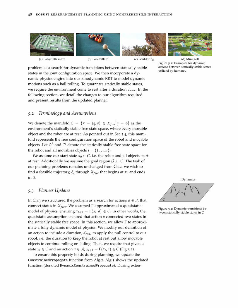
48 robust rearrangement planning using nonprehensile interaction
(a) Labyrinth maze (b) Pool billard (c) Bouldering (d) Mini golfFigure 5.1: Examples for dynamicactions between statically stable statesutilized by humans.
problem as a search for dynamic transitions between statically stablestates in the joint configuration space. We then incorporate a dy-namic physics engine into our kinodynamic RRT to model dynamicmotions such as a ball rolling. To guarantee statically stable states,we require the environment come to rest after a duration Tmax. In thefollowing section, we detail the changes to our algorithm requiredand present results from the updated planner.
5.2 Terminology and Assumptions
We denote the manifold C = {x = (q, q) ∈ X f ree|q = 0} as theenvironment’s statically stable free state space, where every movableobject and the robot are at rest. As pointed out in Sec.3.4, this mani-fold represents the free configuration space of the robot and movableobjects. Let CR and Ci denote the statically stable free state space forthe robot and all movables objects i = {1 . . . m}.
We assume our start state x0 ∈ C, i.e. the robot and all objects startat rest. Additionally we assume the goal region G ⊆ C. The task ofour planning problems remains unchanged from Ch.2: we wish tofind a feasible trajectory, ξ, through X f ree that begins at x0 and endsin G.
5.3 Planner Updates
Dynamics
C
x0
x1x2
x3x4
Figure 5.2: Dynamic transitions be-tween statically stable states in C
In Ch.3 we structured the problem as a search for actions a ∈ A thatconnect states in X f ree. We assumed Γ approximated a quasistaticmodel of physics, ensuring xt+1 = Γ(xt, a) ∈ C. In other words, thequasistatic assumption ensured that action a connected two states inthe statically stable free space. In this section, we allow Γ to approxi-mate a fully dynamic model of physics. We modify our definition ofan action to include a duration, drest, to apply the null control to ourrobot, i.e. the duration to keep the robot at rest but allow movableobjects to continue rolling or sliding. Then, we require that given astate xt ∈ C and an action a ∈ A, xt+1 = Γ(xt, a) ∈ C (Fig.5.2).
To ensure this property holds during planning, we update theConstrainedPropagate function from Alg.2. Alg.5 shows the updatedfunction (denoted DynamicConstrainedPropagate). During exten-
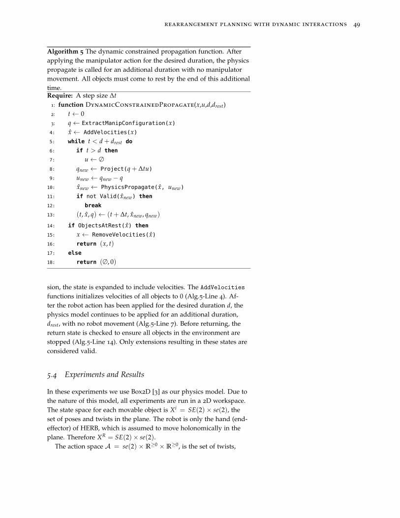
rearrangement planning with dynamic interactions 49
Algorithm 5 The dynamic constrained propagation function. Afterapplying the manipulator action for the desired duration, the physicspropagate is called for an additional duration with no manipulatormovement. All objects must come to rest by the end of this additionaltime.Require: A step size ∆t
1: function DynamicConstrainedPropagate(x,u,d,drest)2: t← 03: q← ExtractManipConfiguration(x)
4: x ← AddVelocities(x)
5: while t < d + drest do
6: if t > d then
7: u← ∅
8: qnew ← Project(q + ∆tu)
9: unew ← qnew − q
10: xnew ← PhysicsPropagate(x, unew)
11: if not Valid(xnew) then
12: break
13: (t, x, q)← (t + ∆t, xnew, qnew)
14: if ObjectsAtRest(x) then
15: x ← RemoveVelocities(x)
16: return (x, t)
17: else
18: return (∅, 0)
sion, the state is expanded to include velocities. The AddVelocities
functions initializes velocities of all objects to 0 (Alg.5-Line 4). Af-ter the robot action has been applied for the desired duration d, thephysics model continues to be applied for an additional duration,drest, with no robot movement (Alg.5-Line 7). Before returning, thereturn state is checked to ensure all objects in the environment arestopped (Alg.5-Line 14). Only extensions resulting in these states areconsidered valid.
5.4 Experiments and Results
In these experiments we use Box2D [3] as our physics model. Due tothe nature of this model, all experiments are run in a 2D workspace.The state space for each movable object is Xi = SE(2) × se(2), theset of poses and twists in the plane. The robot is only the hand (end-effector) of HERB, which is assumed to move holonomically in theplane. Therefore XR = SE(2)× se(2).
The action space A = se(2) × R≥0 × R
≥0, is the set of twists,
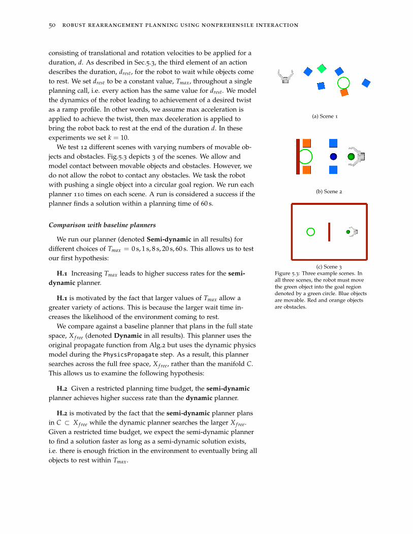
50 robust rearrangement planning using nonprehensile interaction
consisting of translational and rotation velocities to be applied for aduration, d. As described in Sec.5.3, the third element of an actiondescribes the duration, drest, for the robot to wait while objects cometo rest. We set drest to be a constant value, Tmax, throughout a singleplanning call, i.e. every action has the same value for drest. We modelthe dynamics of the robot leading to achievement of a desired twistas a ramp profile. In other words, we assume max acceleration isapplied to achieve the twist, then max deceleration is applied tobring the robot back to rest at the end of the duration d. In theseexperiments we set k = 10.
(a) Scene 1
(b) Scene 2
(c) Scene 3
Figure 5.3: Three example scenes. Inall three scenes, the robot must movethe green object into the goal regiondenoted by a green circle. Blue objectsare movable. Red and orange objectsare obstacles.
We test 12 different scenes with varying numbers of movable ob-jects and obstacles. Fig.5.3 depicts 3 of the scenes. We allow andmodel contact between movable objects and obstacles. However, wedo not allow the robot to contact any obstacles. We task the robotwith pushing a single object into a circular goal region. We run eachplanner 110 times on each scene. A run is considered a success if theplanner finds a solution within a planning time of 60 s.
Comparison with baseline planners
We run our planner (denoted Semi-dynamic in all results) fordifferent choices of Tmax = 0 s, 1 s, 8 s, 20 s, 60 s. This allows us to testour first hypothesis:
H.1 Increasing Tmax leads to higher success rates for the semi-
dynamic planner.
H.1 is motivated by the fact that larger values of Tmax allow agreater variety of actions. This is because the larger wait time in-creases the likelihood of the environment coming to rest.
We compare against a baseline planner that plans in the full statespace, X f ree (denoted Dynamic in all results). This planner uses theoriginal propagate function from Alg.2 but uses the dynamic physicsmodel during the PhysicsPropagate step. As a result, this plannersearches across the full free space, X f ree, rather than the manifold C.This allows us to examine the following hypothesis:
H.2 Given a restricted planning time budget, the semi-dynamic
planner achieves higher success rate than the dynamic planner.
H.2 is motivated by the fact that the semi-dynamic planner plansin C ⊂ X f ree while the dynamic planner searches the larger X f ree.Given a restricted time budget, we expect the semi-dynamic plannerto find a solution faster as long as a semi-dynamic solution exists,i.e. there is enough friction in the environment to eventually bring allobjects to rest within Tmax.
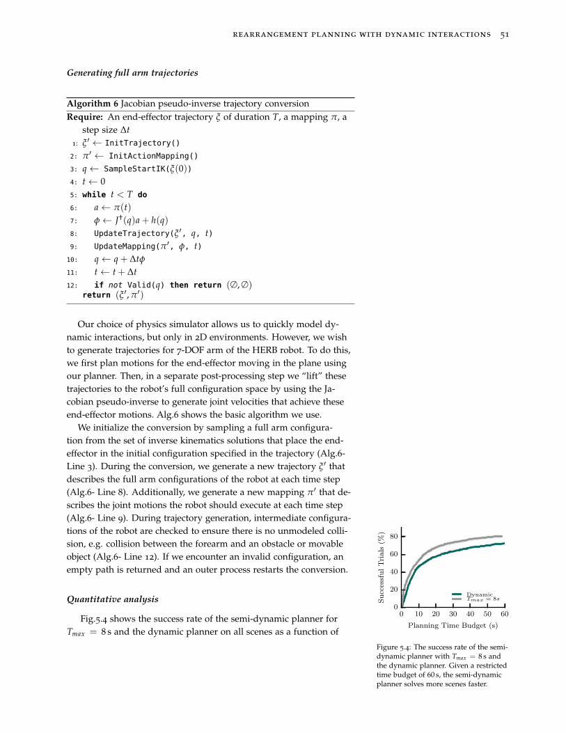
rearrangement planning with dynamic interactions 51
Generating full arm trajectories
Algorithm 6 Jacobian pseudo-inverse trajectory conversionRequire: An end-effector trajectory ξ of duration T, a mapping π, a
step size ∆t
1: ξ ′ ← InitTrajectory()
2: π′ ← InitActionMapping()
3: q← SampleStartIK(ξ(0))4: t← 05: while t < T do
6: a← π(t)
7: φ← J†(q)a + h(q)
8: UpdateTrajectory(ξ ′, q, t)
9: UpdateMapping(π′, φ, t)
10: q← q + ∆tφ
11: t← t + ∆t
12: if not Valid(q) then return (∅, ∅)return (ξ ′, π′)
Our choice of physics simulator allows us to quickly model dy-namic interactions, but only in 2D environments. However, we wishto generate trajectories for 7-DOF arm of the HERB robot. To do this,we first plan motions for the end-effector moving in the plane usingour planner. Then, in a separate post-processing step we “lift” thesetrajectories to the robot’s full configuration space by using the Ja-cobian pseudo-inverse to generate joint velocities that achieve theseend-effector motions. Alg.6 shows the basic algorithm we use.
We initialize the conversion by sampling a full arm configura-tion from the set of inverse kinematics solutions that place the end-effector in the initial configuration specified in the trajectory (Alg.6-Line 3). During the conversion, we generate a new trajectory ξ ′ thatdescribes the full arm configurations of the robot at each time step(Alg.6- Line 8). Additionally, we generate a new mapping π′ that de-scribes the joint motions the robot should execute at each time step(Alg.6- Line 9). During trajectory generation, intermediate configura-tions of the robot are checked to ensure there is no unmodeled colli-sion, e.g. collision between the forearm and an obstacle or movableobject (Alg.6- Line 12). If we encounter an invalid configuration, anempty path is returned and an outer process restarts the conversion.
Quantitative analysis
0 10 20 30 40 50 60
Planning Time Budget (s)
0
20
40
60
80
SuccessfulTrials
(%)
DynamicTmax = 8s
Figure 5.4: The success rate of the semi-dynamic planner with Tmax = 8 s andthe dynamic planner. Given a restrictedtime budget of 60 s, the semi-dynamicplanner solves more scenes faster.
Fig.5.4 shows the success rate of the semi-dynamic planner forTmax = 8 s and the dynamic planner on all scenes as a function of
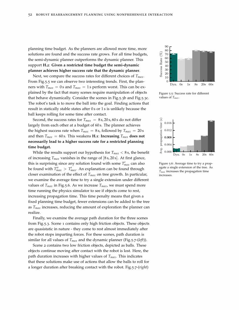
52 robust rearrangement planning using nonprehensile interaction
planning time budget. As the planners are allowed more time, moresolutions are found and the success rate grows. For all time budgets,the semi-dynamic planner outperforms the dynamic planner. Thissupport H.2: Given a restricted time budget the semi-dynamic
planner achieves higher success rate that the dynamic planner.
Dyn. 0s 1s 8s 20s 60s0
102030405060708090
SuccessRate
(%)
Figure 5.5: Success rate for differentvalues of Tmax .
Next, we compare the success rates for different choices of Tmax.From Fig.5.5 we can observe two interesting trends. First, the plan-ners with Tmax = 0 s and Tmax = 1 s perform worst. This can be ex-plained by the fact that many scenes require manipulation of objectsthat behave dynamically. Consider the scenes in Fig.5.3b and Fig.5.3c.The robot’s task is to move the ball into the goal. Finding actions thatresult in statically stable states after 0 s or 1 s is unlikely because theball keeps rolling for some time after contact.
Second, the success rates for Tmax = 8 s, 20 s, 60 s do not differlargely from each other at a budget of 60 s. The planner achievesthe highest success rate when Tmax = 8 s, followed by Tmax = 20 sand then Tmax = 60 s. This weakens H.1: Increasing Tmax does not
necessarily lead to a higher success rate for a restricted planning
time budget.
Dyn. 0s 1s 8s 20s 60s0.000
0.004
0.0080.008
0.012
0.016
Avg.propagationtime(s)
Figure 5.6: Average time to try a prop-agate a single extension of the tree. AsTmax increases the propagation timeincreases.
While the results support our hypothesis for Tmax < 8 s, the benefitof increasing Tmax vanishes in the range of [8 s, 20 s]. At first glance,this is surprising since any solution found with some T′max can alsobe found with T′′max > T′max. An explanation can be found throughcloser examination of the effect of Tmax on tree growth. In particular,we examine the average time to try a single extension under differentvalues of Tmax in Fig.5.6. As we increase Tmax, we must spend moretime running the physics simulator to see if objects come to rest,increasing propagation time. This time penalty means that given afixed planning time budget, fewer extensions can be added to the treeas Tmax increases, reducing the amount of exploration the planner canrealize.
Finally, we examine the average path duration for the three scenesfrom Fig.5.3. Scene 1 contains only high friction objects. These objectsare quasistatic in nature - they come to rest almost immediately afterthe robot stops imparting forces. For these scenes, path duration issimilar for all values of Tmax and the dynamic planner (Fig.5.7-(left)).
Scene 2 contains two low friction objects, depicted as balls. Theseobjects continue moving after contact with the robot is lost. Here, thepath duration increases with higher values of Tmax. This indicatesthat these solutions make use of actions that allow the balls to roll fora longer duration after breaking contact with the robot. Fig.5.7-(right)
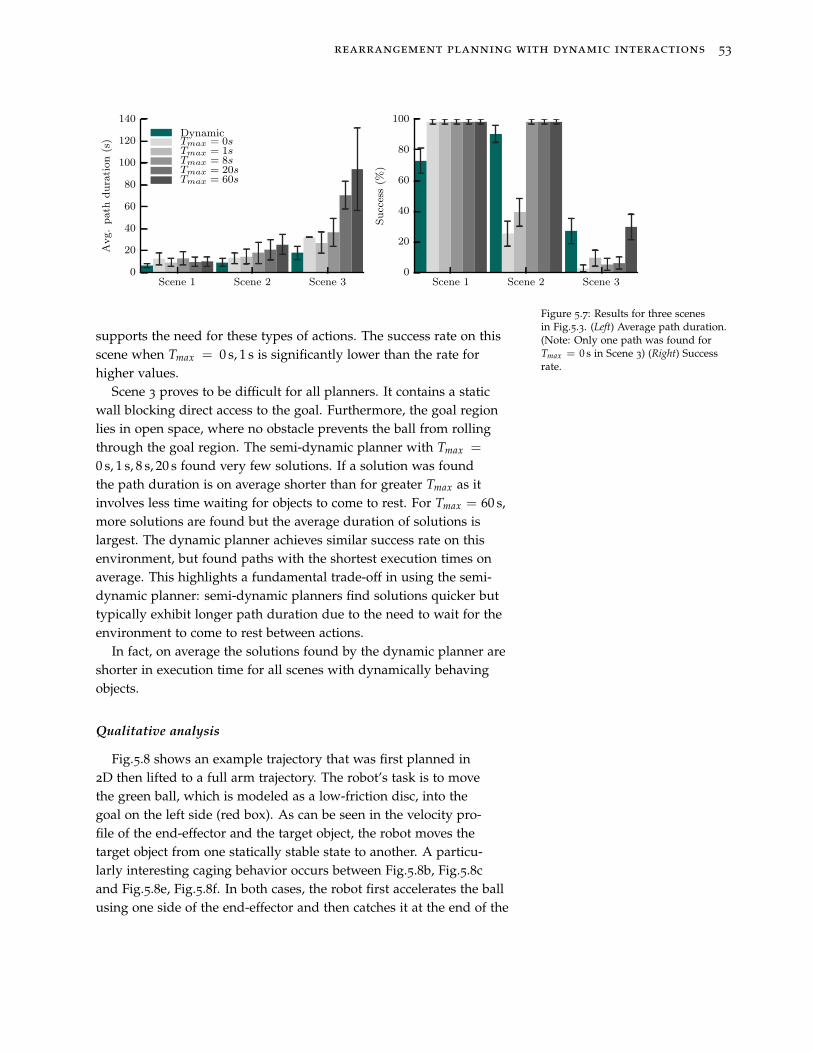
rearrangement planning with dynamic interactions 53
Scene 1 Scene 2 Scene 30
20
40
60
80
100
120
140Avg.path
duration(s)
DynamicTmax = 0sTmax = 1sTmax = 8sTmax = 20sTmax = 60s
Scene 1 Scene 2 Scene 30
20
40
60
80
100
Success(%
)
Figure 5.7: Results for three scenesin Fig.5.3. (Left) Average path duration.(Note: Only one path was found forTmax = 0 s in Scene 3) (Right) Successrate.
supports the need for these types of actions. The success rate on thisscene when Tmax = 0 s, 1 s is significantly lower than the rate forhigher values.
Scene 3 proves to be difficult for all planners. It contains a staticwall blocking direct access to the goal. Furthermore, the goal regionlies in open space, where no obstacle prevents the ball from rollingthrough the goal region. The semi-dynamic planner with Tmax =
0 s, 1 s, 8 s, 20 s found very few solutions. If a solution was foundthe path duration is on average shorter than for greater Tmax as itinvolves less time waiting for objects to come to rest. For Tmax = 60 s,more solutions are found but the average duration of solutions islargest. The dynamic planner achieves similar success rate on thisenvironment, but found paths with the shortest execution times onaverage. This highlights a fundamental trade-off in using the semi-dynamic planner: semi-dynamic planners find solutions quicker buttypically exhibit longer path duration due to the need to wait for theenvironment to come to rest between actions.
In fact, on average the solutions found by the dynamic planner areshorter in execution time for all scenes with dynamically behavingobjects.
Qualitative analysis
Fig.5.8 shows an example trajectory that was first planned in2D then lifted to a full arm trajectory. The robot’s task is to movethe green ball, which is modeled as a low-friction disc, into thegoal on the left side (red box). As can be seen in the velocity pro-file of the end-effector and the target object, the robot moves thetarget object from one statically stable state to another. A particu-larly interesting caging behavior occurs between Fig.5.8b, Fig.5.8cand Fig.5.8e, Fig.5.8f. In both cases, the robot first accelerates the ballusing one side of the end-effector and then catches it at the end of the

54 robust rearrangement planning using nonprehensile interaction
(a) (b) (c) (d)* (e) (f)
(g) (h)* (i) (j) (k) (l)*
0 2 4 6 8 100.00
0.10
0.20
0.30
0.40(l)*(c) (d)*(a)(b) (e) (f) (g) (h)* (i) (j) (k)
Vel
oci
ty (
m/
s)
Time (s)
ManipulatorBall
Vel
oci
ty (
m/
s)
Time (s)
Manipulator
Ball
Figure 5.8: Top: Snapshots from a semi-dynamic trajectory lifted to a 7-DOFarm trajectory and executed on therobot in simulation (Tmax = 8s). Thetask is to move the green ball into thered goal. The orange boxes are staticobstacles. The states marked with ∗are statically stable. Middle: Velocityprofile of the end-effector and thetarget. Note how the robot waits untilthe ball comes to rest before it performsthe next action. Bottom: Velocities fora dynamic trajectory for the samescene. In contrast to the semi-dynamictrajectory the environment does notcome to rest after each action.
action using the other side of the end-effector. We observed this be-havior frequently in many scenes. An action where the robot pushesa ball into open space is less likely to lead to a statically stable statewithin Tmax than an action for which caging occurs.
Fig.5.8-bottom shows the velocity profile for a trajectory plannedwith the dynamic planner on the same scene. Note how both themanipulator and the target object keep in motion for the whole tra-jectory. As a result the total duration of the trajectory is shorter thanthe semi-dynamic one.
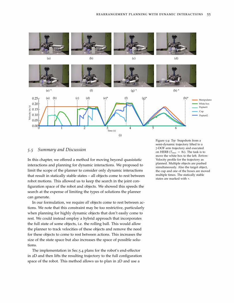
rearrangement planning with dynamic interactions 55
(a) (b) (c) (d)
(e) * (f) (g) * (h) *
0 1 2 3 4 5 60.00
0.05
0.10
0.15
0.20
0.25 (a) (b) (c) (d) (e)* (f) (g)* (h)*
Vel
oci
ty (
m/
s)
Time (s)
Manipulator
White box
Poptart1
Poptart2
Cup
(i)
Figure 5.9: Top: Snapshots from asemi-dynamic trajectory lifted to a7-DOF arm trajectory and executedon HERB (Tmax = 8s). The task is tomove the white box to the left. Bottom:Velocity profile for the trajectory asplanned. Multiple objects are pushedsimultaneously. Also the target object,the cup and one of the boxes are movedmultiple times. The statically stablestates are marked with ∗.
5.5 Summary and Discussion
In this chapter, we offered a method for moving beyond quasistaticinteractions and planning for dynamic interactions. We proposed tolimit the scope of the planner to consider only dynamic interactionsthat result in statically stable states – all objects come to rest betweenrobot motions. This allowed us to keep the search in the joint con-figuration space of the robot and objects. We showed this speeds thesearch at the expense of limiting the types of solutions the plannercan generate.
In our formulation, we require all objects come to rest between ac-tions. We note that this constraint may be too restrictive, particularlywhen planning for highly dynamic objects that don’t easily come torest. We could instead employ a hybrid approach that incorporatesthe full state of some objects, i.e. the rolling ball. This would allowthe planner to track velocities of these objects and remove the needfor these objects to come to rest between actions. This increases thesize of the state space but also increases the space of possible solu-tions.
The implementation in Sec.5.4 plans for the robot’s end-effectorin 2D and then lifts the resulting trajectory to the full configurationspace of the robot. This method allows us to plan in 2D and use a
56 robust rearrangement planning using nonprehensile interaction
fast physics model. However, it introduces two main limitations.First, by planning in 2D we are unable to take into account the kine-matics of the arm at plan time. As a result, the planner can produceend-effector trajectories that are kinematically infeasible. When thesetrajectories are encountered, they are discarded and the planner isrestarted.
Second, any contact between the arm and objects is not modeled.Again, this can lead the planner to produce infeasible trajectories,i.e. there exist no collision-free arm motions that realize the end-effector motion. In the previous chapters, we have shown that allow-ing contact between the full robot and objects proves beneficial to theplanner by expanding the space of solutions that can be achieved. Inorder to allow these trajectories, we must substitute a full 3D physicsmodel. This will result in overall slower tree extension, but at theadded benefit of an expanded solution set.
Despite these limitations, our preliminary experiments show weare able to produce executable trajectories on a real robot (Fig.5.9).While we are able to achieve some success executing these trajectoriesopen-loop, the dynamic interactions highlight the need to incorpo-rate uncertainty into our planner. It is impossible to perfectly modelthe dynamic interactions, especially with low friction objects like therolling ball. As a result, many of our executions of scenes with suchobjects resulted in failure. In Part II, we will present methods for in-corporating the uncertainties prevalent in our real physical systems.
Part II
Rearrangement Planning
under Uncertainty

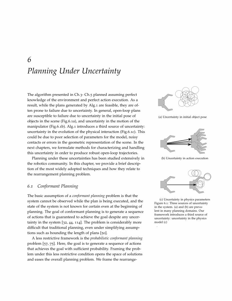
6
Planning Under Uncertainty
The algorithm presented in Ch.3- Ch.5 planned assuming perfectknowledge of the environment and perfect action execution. As aresult, while the plans generated by Alg.1 are feasible, they are of-ten prone to failure due to uncertainty. In general, open-loop plansare susceptible to failure due to uncertainty in the initial pose ofobjects in the scene (Fig.6.1a), and uncertainty in the motion of themanipulator (Fig.6.1b). Alg.1 introduces a third source of uncertainty:uncertainty in the evolution of the physical interaction (Fig.6.1c). Thiscould be due to poor selection of parameters for the model, noisycontacts or errors in the geometric representation of the scene. In thenext chapters, we formulate methods for characterizing and handlingthis uncertainty in order to produce robust open-loop trajectories.
(a) Uncertainty in initial object pose
(b) Uncertainty in action execution
(c) Uncertainty in physics parametersFigure 6.1: Three sources of uncertaintyin the system. (a) and (b) are preva-lent in many planning domains. Ourframework introduces a third source ofuncertainty: uncertainty in the physicsmodel (c)
.
Planning under these uncertainties has been studied extensively inthe robotics community. In this chapter, we provide a brief descrip-tion of the most widely adopted techniques and how they relate tothe rearrangement planning problem.
6.1 Conformant Planning
The basic assumption of a conformant planning problem is that thesystem cannot be observed while the plan is being executed, and thestate of the system is not known for certain even at the beginning ofplanning. The goal of conformant planning is to generate a sequenceof actions that is guaranteed to achieve the goal despite any uncer-tainty in the system [32, 44, 114]. The problem is considerably moredifficult that traditional planning, even under simplifying assump-tions such as bounding the length of plans [50].
A less restrictive framework is the probabilistic conformant planning
problem [57, 75]. Here, the goal is to generate a sequence of actionsthat achieves the goal with sufficient probability. Framing the prob-lem under this less restrictive condition opens the space of solutionsand eases the overall planning problem. We frame the rearrange-
60 robust rearrangement planning using nonprehensile interaction
ment planning problem as an instance of probabilistic conformantplanning in Ch.7.
6.2 Sampling Based Approaches
Some works have proposed methods that extend sampling basedframeworks to solve the probabilistic planning problem. One of themost common approaches is to build on the Probabilistic Roadmap(PRM) algorithm [62] by accounting for stochasticity in robot pose [106],transition dynamics [10] and obstacle representation [47]. While theuse of a PRM is infeasible for this problem, we borrow some key in-spirations from these works. In particular, in Ch.8 we propose to useMonte Carlo simulations to estimate the probability a sequence ofactions achieves success. This same method is employed to estimatesuccess of individual actions in [10].
Alternate works have built uncertainty into RRTs [83, 93, 101] un-der assumptions such as bounded uncertainty. Indeed, we couldmodify our algorithms from Part I so that each node representsa set of possible states, or belief state, rather than a single knownstate. The difficulty arises in defining an informative distance met-ric between two belief states that allows us to effectively guide treegrowth [80]. We provide two methods of incorporating uncertaintyinto RRTs in Ch.9.
6.3 Partially Observable Markov Decision Processes
An alternative and common method of handling planning underuncertainty is to formulate the problem as a Partially ObservableMarkov Decision Process (POMDP). POMDP solvers can reasonabout uncertainty and incorporate closed-loop feedback from local orglobal sensors. We refer the reader to one of several good surveys ofthe formulation, theory and algorithms [27, 82, 95, 124].
We are interested in a sub-domain of POMDP problems: Un-observable Markov Decision Process (UMDP). In these problems,the robot does not receive observations that help determine state.While the lack of observations reduces the complexity, the problemis still difficult to solve exactly, particularly in our continuous stateand action space with non-Gaussian non-smooth distributions. Inthis work we consider online solvers that find approximate solu-tions [13, 74, 111, 121]. We use an algorithm inspired by Partially Ob-servable Monte Carlo Planning (POMCP) [111] which relies on MonteCarlo simulations to estimate our difficult distributions in Ch.10.
planning under uncertainty 61
6.4 Rearrangement Planning under Uncertainty
A few works have considered uncertainty in planning among mov-able objects. Levihn et al. [78] formulate the problem as a MarkovDecision Problem and uses the Box2D physics simulator to estimatetransition probabilities between states. The proposed planner uses ahierarchical approach, using the MDP to plan high-level actions thatconnect regions of free state space by moving objects, then using astate space planner to generate geometrically feasible instantiations ofthese actions. An alternative backtracking-based approach is used tosolve rearrangement planning under uncertainty in [36].
Neither of these approaches can be applied directly to our prob-lem without restricting the space of solutions our planner can con-sider. The complexity of tracking free space [78] is difficult for thehigh-dimensional robot state spaces we consider. The backtrackingapproach [36] limits object interaction to a single object at a time.However, we draw inspiration from both of these approaches in thesolutions we present in the following sections.

7
Incorporating Uncertainty into Rearrangement Plan-
ning
Formally, we will augment the problem described in Ch.2. Ratherthan planning from a deterministic start state x0 ∈ X f ree we insteadbegin in an initial belief state b0 = p(x0) that is a probability distri-bution over the start state. Additionally we assume our state evolvesas a stochastic non-holonomic system. Thus we have a distributionp(ξ|π) of trajectories that results from starting in x0 ∼ b0 and ex-ecuting control inputs π under the stochastic transition dynamics.Our goal is to find a sequence of control inputs π that maximizesthe probability pπ = Pr[Λ[ξ] = 1] of satisfying the success functional
Λ : Ξ → {0, 1} where Ξ is the set of all trajectories. We define thesuccess functional
Λ[ξ] =
1 : ξ(Tξ) ∈ XG
0 : otherwise(7.1)
where Tξ is the duration of trajectory ξ.This problem is particularly hard for rearrangement planning.
First, the problem is set in a high-dimensional space with continu-ous controls. Second, contact causes physics to evolve in complex,non-linear ways and quickly leads to multimodal and non-smoothdistributions [68, 70, 104]. Third, finding good trajectories is inher-ently hard: most trajectories achieve success with zero probability.
In the following chapters, we outline methods for handling uncer-tainty under the challenges presented by rearrangement planning.

8
Trajectory Selection for Rearrangement Planning
This chapter is adapted from Koval etal. [69] and contains work completed incollaboration with Michael Koval.
In this chapter we formulate rearrangement planning under uncer-tainty as a selection problem. To do this we take advantage of threecharacteristics of the planning framework presented in Part I: (1) themethod for generating trajectories is stochastic – several calls to theplanner for the same query will result in different trajectories, (2) theuse of a physics model allows us to easily forward-simulate the sys-tem’s dynamics under different initial conditions, and (3) we can testwhether a simulation is successful, i.e. achieves the goal.
Given these properties we first use the stochastic planner to gen-erate a finite set of state space trajectory candidates. We then performseveral noisy rollouts: forward-simulations under varying initial con-ditions. We use the success or failure of these rollouts to form anestimate of pπ , the probability of the trajectory being successfullyexecuted on the real robot, and use this estimate to select the mostrobust trajectory.
Given a set of k trajectories, we could perform a fixed sufficientnumber n of rollouts on each trajectory, requiring a total of kn roll-outs. However, rollouts are computationally expensive, requiring theevaluation of a full physics simulation. We seek an algorithm that canefficiently choose the best trajectory given a small rollout budget.
We can formalize this selection problem as an instance of the “bestarm” variant [90] of the k-armed bandit problem [107]. In our for-mulation, each candidate trajectory is an “arm” and the goal is toidentify the best arm given a fixed budget of rollouts. We use thesuccessive rejects algorithm [11] to select the best candidate. In thefollowing sections we detail important components of the method.
8.1 Trajectory Selection
Our goal is to find the most robust sequence of control inputs:
πbest = argmaxπ∈Π
pπ (8.1)
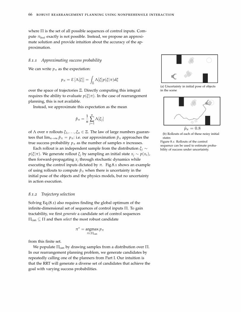
66 robust rearrangement planning using nonprehensile interaction
where Π is the set of all possible sequences of control inputs. Com-pute πbest exactly is not possible. Instead, we propose an approxi-mate solution and provide intuition about the accuracy of the ap-proximation.
8.1.1 Approximating success probability
We can write pπ as the expectation:
pπ = E [Λ[ξ]] =∫
ΞΛ[ξ]p(ξ|π)dξ
over the space of trajectories Ξ. Directly computing this integralrequires the ability to evaluate p(ξ|π). In the case of rearrangementplanning, this is not available.
(a) Uncertainty in initial pose of objectsin the scene
(b) Rollouts of each of these noisy initialstates
Figure 8.1: Rollouts of the controlsequence can be used to estimate proba-bility of success under uncertainty.
Instead, we approximate this expectation as the mean
pπ =1n
n
∑j=1
Λ[ξ j]
of Λ over n rollouts ξ1, . . . , ξn ∈ Ξ. The law of large numbers guaran-tees that limn→∞ pπ = pπ : i.e. our approximation pπ approaches thetrue success probability pπ as the number of samples n increases.
Each rollout is an independent sample from the distribution ξ j ∼
p(ξ|π). We generate rollout ξ j by sampling an initial state xj ∼ p(xs),then forward-propagating xj through stochastic dynamics whileexecuting the control inputs dictated by π. Fig.8.1 shows an exampleof using rollouts to compute pπ when there is uncertainty in theinitial pose of the objects and the physics models, but no uncertaintyin action execution.
8.1.2 Trajectory selection
Solving Eq.(8.1) also requires finding the global optimum of theinfinite-dimensional set of sequences of control inputs Π. To gaintractability, we first generate a candidate set of control sequencesΠcan ⊆ Π and then select the most robust candidate
π∗ = argmaxπ∈Πcan
pπ
from this finite set.We populate Πcan by drawing samples from a distribution over Π.
In our rearrangement planning problem, we generate candidates byrepeatedly calling one of the planners from Part I. Our intuition isthat the RRT will generate a diverse set of candidates that achieve thegoal with varying success probabilities.
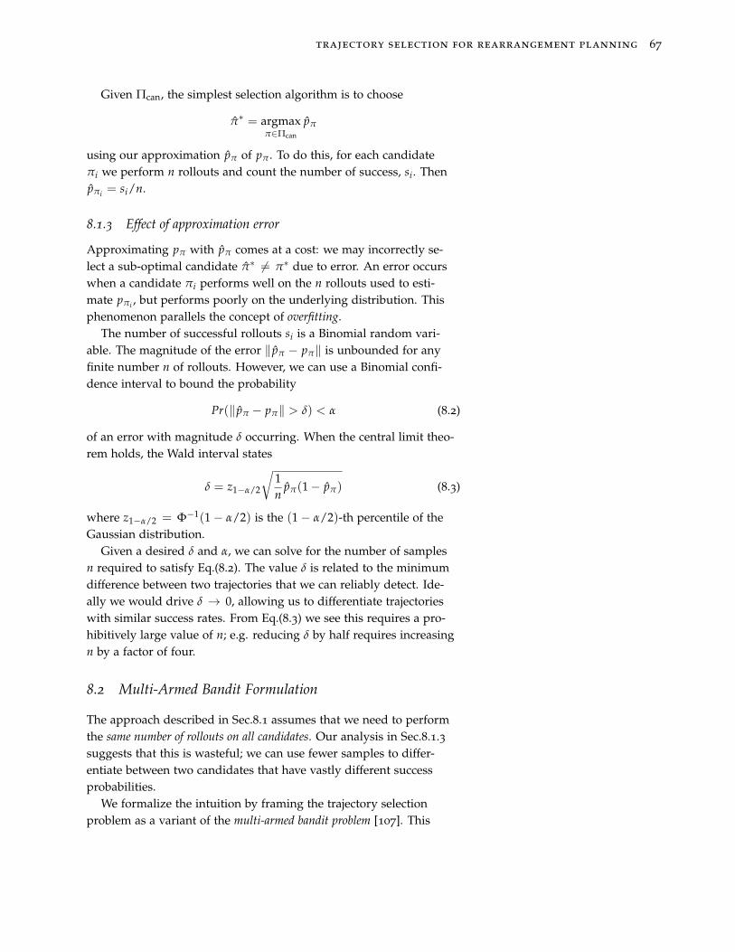
trajectory selection for rearrangement planning 67
Given Πcan, the simplest selection algorithm is to choose
π∗ = argmaxπ∈Πcan
pπ
using our approximation pπ of pπ . To do this, for each candidateπi we perform n rollouts and count the number of success, si. Thenpπi
= si/n.
8.1.3 Effect of approximation error
Approximating pπ with pπ comes at a cost: we may incorrectly se-lect a sub-optimal candidate π∗ 6= π∗ due to error. An error occurswhen a candidate πi performs well on the n rollouts used to esti-mate pπi
, but performs poorly on the underlying distribution. Thisphenomenon parallels the concept of overfitting.
The number of successful rollouts si is a Binomial random vari-able. The magnitude of the error ‖ pπ − pπ‖ is unbounded for anyfinite number n of rollouts. However, we can use a Binomial confi-dence interval to bound the probability
Pr(‖ pπ − pπ‖ > δ) < α (8.2)
of an error with magnitude δ occurring. When the central limit theo-rem holds, the Wald interval states
δ = z1−α/2
√
1n
pπ(1− pπ) (8.3)
where z1−α/2 = Φ−1(1− α/2) is the (1− α/2)-th percentile of theGaussian distribution.
Given a desired δ and α, we can solve for the number of samplesn required to satisfy Eq.(8.2). The value δ is related to the minimumdifference between two trajectories that we can reliably detect. Ide-ally we would drive δ → 0, allowing us to differentiate trajectorieswith similar success rates. From Eq.(8.3) we see this requires a pro-hibitively large value of n; e.g. reducing δ by half requires increasingn by a factor of four.
8.2 Multi-Armed Bandit Formulation
The approach described in Sec.8.1 assumes that we need to performthe same number of rollouts on all candidates. Our analysis in Sec.8.1.3suggests that this is wasteful; we can use fewer samples to differ-entiate between two candidates that have vastly different successprobabilities.
We formalize the intuition by framing the trajectory selectionproblem as a variant of the multi-armed bandit problem [107]. This
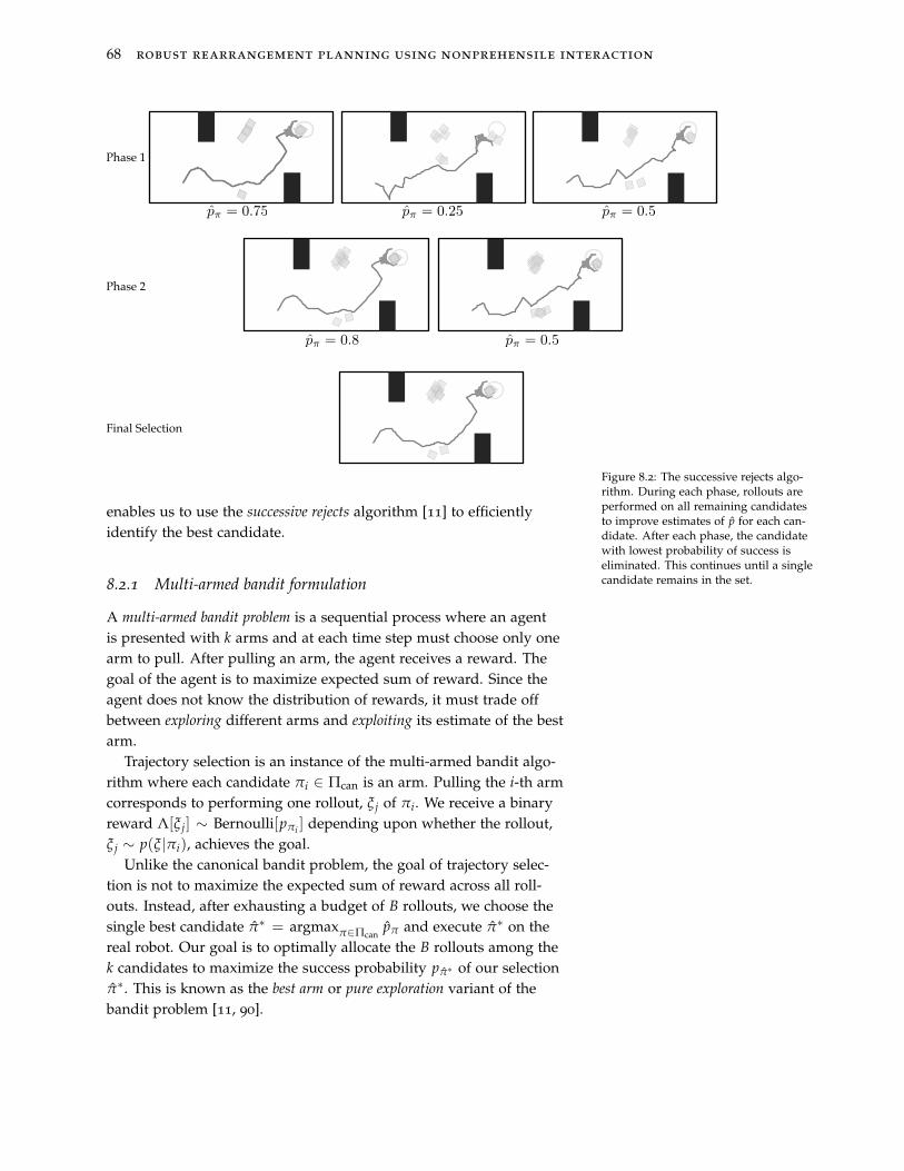
68 robust rearrangement planning using nonprehensile interaction
Phase 1
Phase 2
Final Selection
Figure 8.2: The successive rejects algo-rithm. During each phase, rollouts areperformed on all remaining candidatesto improve estimates of p for each can-didate. After each phase, the candidatewith lowest probability of success iseliminated. This continues until a singlecandidate remains in the set.
enables us to use the successive rejects algorithm [11] to efficientlyidentify the best candidate.
8.2.1 Multi-armed bandit formulation
A multi-armed bandit problem is a sequential process where an agentis presented with k arms and at each time step must choose only onearm to pull. After pulling an arm, the agent receives a reward. Thegoal of the agent is to maximize expected sum of reward. Since theagent does not know the distribution of rewards, it must trade offbetween exploring different arms and exploiting its estimate of the bestarm.
Trajectory selection is an instance of the multi-armed bandit algo-rithm where each candidate πi ∈ Πcan is an arm. Pulling the i-th armcorresponds to performing one rollout, ξ j of πi. We receive a binaryreward Λ[ξ j] ∼ Bernoulli[pπi
] depending upon whether the rollout,ξ j ∼ p(ξ|πi), achieves the goal.
Unlike the canonical bandit problem, the goal of trajectory selec-tion is not to maximize the expected sum of reward across all roll-outs. Instead, after exhausting a budget of B rollouts, we choose thesingle best candidate π∗ = argmaxπ∈Πcan
pπ and execute π∗ on thereal robot. Our goal is to optimally allocate the B rollouts among thek candidates to maximize the success probability pπ∗ of our selectionπ∗. This is known as the best arm or pure exploration variant of thebandit problem [11, 90].
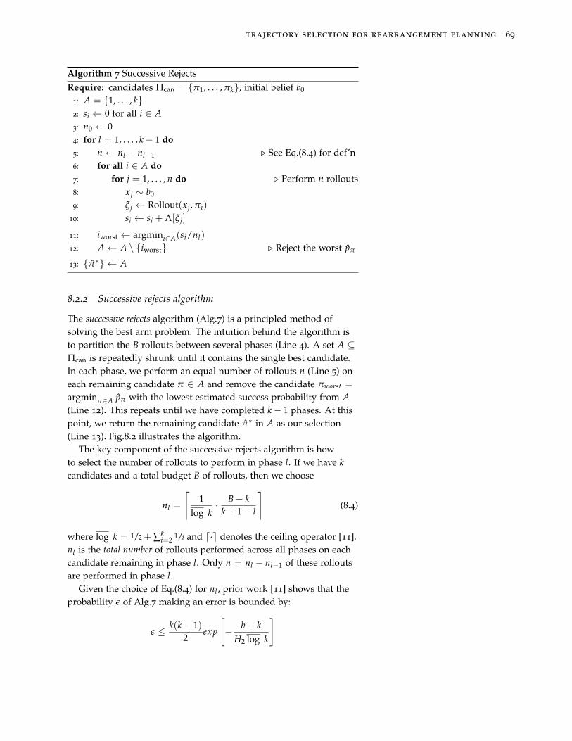
trajectory selection for rearrangement planning 69
Algorithm 7 Successive Rejects
Require: candidates Πcan = {π1, . . . , πk}, initial belief b0
1: A = {1, . . . , k}
2: si ← 0 for all i ∈ A
3: n0 ← 04: for l = 1, . . . , k− 1 do
5: n← nl − nl−1 ⊲ See Eq.(8.4) for def’n6: for all i ∈ A do
7: for j = 1, . . . , n do ⊲ Perform n rollouts8: xj ∼ b0
9: ξ j ← Rollout(xj, πi)
10: si ← si + Λ[ξ j]
11: iworst ← argmini∈A(si/nl)
12: A← A \ {iworst} ⊲ Reject the worst pπ
13: {π∗} ← A
8.2.2 Successive rejects algorithm
The successive rejects algorithm (Alg.7) is a principled method ofsolving the best arm problem. The intuition behind the algorithm isto partition the B rollouts between several phases (Line 4). A set A ⊆
Πcan is repeatedly shrunk until it contains the single best candidate.In each phase, we perform an equal number of rollouts n (Line 5) oneach remaining candidate π ∈ A and remove the candidate πworst =
argminπ∈A pπ with the lowest estimated success probability from A
(Line 12). This repeats until we have completed k− 1 phases. At thispoint, we return the remaining candidate π∗ in A as our selection(Line 13). Fig.8.2 illustrates the algorithm.
The key component of the successive rejects algorithm is howto select the number of rollouts to perform in phase l. If we have k
candidates and a total budget B of rollouts, then we choose
nl =
⌈
1
log k·
B− k
k + 1− l
⌉
(8.4)
where log k = 1/2 + ∑ki=2
1/i and ⌈·⌉ denotes the ceiling operator [11].nl is the total number of rollouts performed across all phases on eachcandidate remaining in phase l. Only n = nl − nl−1 of these rolloutsare performed in phase l.
Given the choice of Eq.(8.4) for nl , prior work [11] shows that theprobability ǫ of Alg.7 making an error is bounded by:
ǫ ≤k(k− 1)
2exp
[
−b− k
H2 log k
]
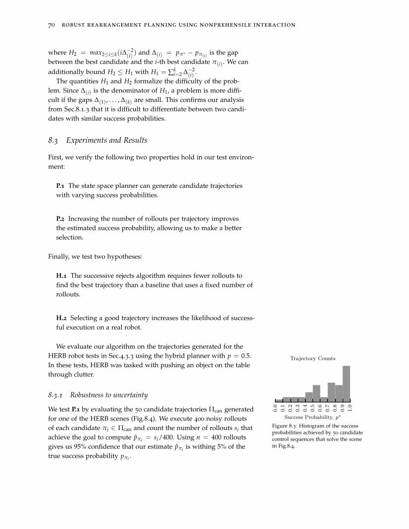
70 robust rearrangement planning using nonprehensile interaction
where H2 = max2≤i≤k(i∆−2(i)
) and ∆(i) = pπ∗ − pπ(i)is the gap
between the best candidate and the i-th best candidate π(i). We can
additionally bound H2 ≤ H1 with H1 = ∑ki=2 ∆−2
(i).
The quantities H1 and H2 formalize the difficulty of the prob-lem. Since ∆(i) is the denominator of H1, a problem is more diffi-cult if the gaps ∆(1), . . . , ∆(k) are small. This confirms our analysisfrom Sec.8.1.3 that it is difficult to differentiate between two candi-dates with similar success probabilities.
8.3 Experiments and Results
First, we verify the following two properties hold in our test environ-ment:
P.1 The state space planner can generate candidate trajectorieswith varying success probabilities.
P.2 Increasing the number of rollouts per trajectory improvesthe estimated success probability, allowing us to make a betterselection.
Finally, we test two hypotheses:
H.1 The successive rejects algorithm requires fewer rollouts tofind the best trajectory than a baseline that uses a fixed number ofrollouts.
H.2 Selecting a good trajectory increases the likelihood of success-ful execution on a real robot.
We evaluate our algorithm on the trajectories generated for theHERB robot tests in Sec.4.3.3 using the hybrid planner with p = 0.5.In these tests, HERB was tasked with pushing an object on the tablethrough clutter.
8.3.1 Robustness to uncertainty
0.0
0.1
0.2
0.3
0.4
0.5
0.6
0.7
0.8
0.9
1.0
Success Probability, p∗
Trajectory Counts
Figure 8.3: Histogram of the successprobabilities achieved by 50 candidatecontrol sequences that solve the scenein Fig.8.4.
We test P.1 by evaluating the 50 candidate trajectories Πcan generatedfor one of the HERB scenes (Fig.8.4). We execute 400 noisy rolloutsof each candidate πi ∈ Πcan and count the number of rollouts si thatachieve the goal to compute pπi
= si/400. Using n = 400 rolloutsgives us 95% confidence that our estimate pπi
is withing 5% of thetrue success probability pπi
.
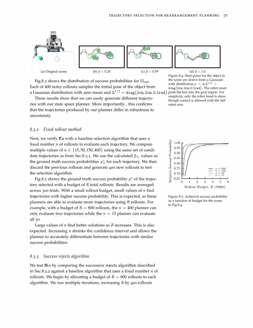
trajectory selection for rearrangement planning 71
(a) Original scene (b) p = 0.28 (c) p = 0.59 (d) p = 1.0Figure 8.4: Start poses for the object inthe scene are drawn from a Gaussianwith distribution µ = 0, Σ1/2 =diag{2cm, 2cm, 0.1rad}. The robot mustpush the box into the goal region. Forsimplicity, only the robot hand is show,though contact is allowed with the fullrobot arm.
Fig.8.3 shows the distribution of success probabilities for Πcan.Each of 400 noisy rollouts samples the initial pose of the object froma Gaussian distribution with zero mean and Σ1/2 = diag{2cm, 2cm, 0.1rad}.
These results show that we can easily generate different trajecto-ries with our state space planner. More importantly , this confirmsthat the trajectories produced by our planner differ in robustness touncertainty.
8.3.2 Fixed rollout method
Nest, we verify P.2 with a baseline selection algorithm that uses afixed number n of rollouts to evaluate each trajectory. We comparemultiple values of n ∈ {15, 50, 150, 400} using the same set of candi-date trajectories as from Sec.8.3.1. We use the calculated pπi
values asthe ground truth success probabilities p∗π for each trajectory. We thendiscard the previous rollouts and generate 400 new rollouts to testthe selection algorithm.
0 1 2 3 4 5 6
Rollout Budget, B (1000s)
0.65
0.70
0.75
0.80
0.85
0.90
0.95
1.00
RelativeSuccessProbability
n = 400n = 150n = 50n = 15
Figure 8.5: Achieved success probabilityas a function of budget for the scenein Fig.8.4.
Fig.8.5 shows the ground truth success probability p∗ of the trajec-tory selected with a budget of B total rollouts. Results are averagedacross 300 trials. With a small rollout budget, small values of n findtrajectories with higher success probability. This is expected, as theseplanners are able to evaluate more trajectories using B rollouts. Forexample, with a budget of B = 800 rollouts, the n = 400 planner canonly evaluate two trajectories while the n = 15 planner can evaluateall 50.
Large values of n find better solutions as B increases. This is alsoexpected. Increasing n shrinks the confidence interval and allows theplanner to accurately differentiate between trajectories with similarsuccess probabilities.
8.3.3 Success rejects algorithm
We test H.1 by comparing the successive rejects algorithm describedin Sec.8.2.2 against a baseline algorithm that uses a fixed number n ofrollouts. We begin by allocating a budget of B = 800 rollouts to eachalgorithm. We run multiple iterations, increasing B by 400 rollouts
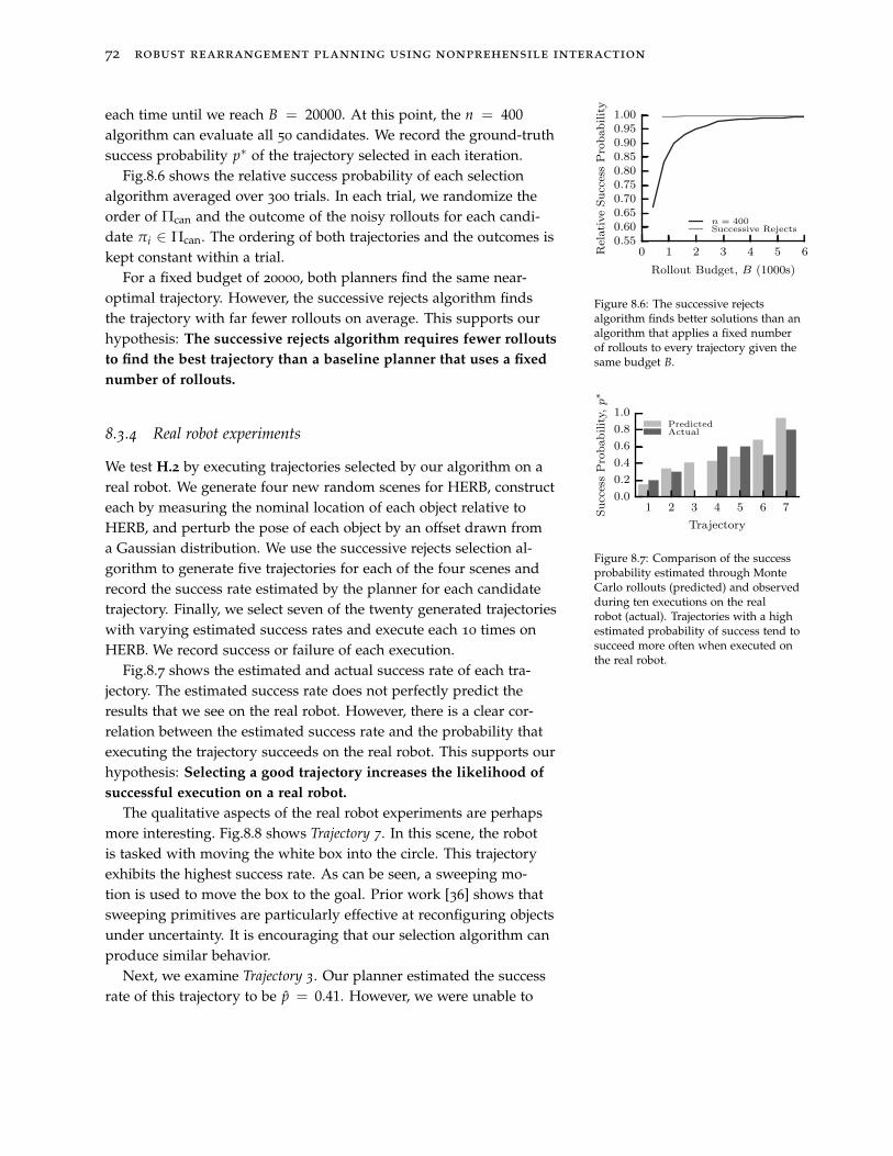
72 robust rearrangement planning using nonprehensile interaction
each time until we reach B = 20000. At this point, the n = 400algorithm can evaluate all 50 candidates. We record the ground-truthsuccess probability p∗ of the trajectory selected in each iteration.
0 1 2 3 4 5 6
Rollout Budget, B (1000s)
0.550.600.650.700.750.800.850.900.951.00
RelativeSuccessProbability
n = 400Successive Rejects
Figure 8.6: The successive rejectsalgorithm finds better solutions than analgorithm that applies a fixed numberof rollouts to every trajectory given thesame budget B.
Fig.8.6 shows the relative success probability of each selectionalgorithm averaged over 300 trials. In each trial, we randomize theorder of Πcan and the outcome of the noisy rollouts for each candi-date πi ∈ Πcan. The ordering of both trajectories and the outcomes iskept constant within a trial.
For a fixed budget of 20000, both planners find the same near-optimal trajectory. However, the successive rejects algorithm findsthe trajectory with far fewer rollouts on average. This supports ourhypothesis: The successive rejects algorithm requires fewer rollouts
to find the best trajectory than a baseline planner that uses a fixed
number of rollouts.
8.3.4 Real robot experiments
1 2 3 4 5 6 7
Trajectory
0.0
0.2
0.4
0.6
0.8
1.0
SuccessProbability,
p∗
PredictedActual
Figure 8.7: Comparison of the successprobability estimated through MonteCarlo rollouts (predicted) and observedduring ten executions on the realrobot (actual). Trajectories with a highestimated probability of success tend tosucceed more often when executed onthe real robot.
We test H.2 by executing trajectories selected by our algorithm on areal robot. We generate four new random scenes for HERB, constructeach by measuring the nominal location of each object relative toHERB, and perturb the pose of each object by an offset drawn froma Gaussian distribution. We use the successive rejects selection al-gorithm to generate five trajectories for each of the four scenes andrecord the success rate estimated by the planner for each candidatetrajectory. Finally, we select seven of the twenty generated trajectorieswith varying estimated success rates and execute each 10 times onHERB. We record success or failure of each execution.
Fig.8.7 shows the estimated and actual success rate of each tra-jectory. The estimated success rate does not perfectly predict theresults that we see on the real robot. However, there is a clear cor-relation between the estimated success rate and the probability thatexecuting the trajectory succeeds on the real robot. This supports ourhypothesis: Selecting a good trajectory increases the likelihood of
successful execution on a real robot.
The qualitative aspects of the real robot experiments are perhapsmore interesting. Fig.8.8 shows Trajectory 7. In this scene, the robotis tasked with moving the white box into the circle. This trajectoryexhibits the highest success rate. As can be seen, a sweeping mo-tion is used to move the box to the goal. Prior work [36] shows thatsweeping primitives are particularly effective at reconfiguring objectsunder uncertainty. It is encouraging that our selection algorithm canproduce similar behavior.
Next, we examine Trajectory 3. Our planner estimated the successrate of this trajectory to be p = 0.41. However, we were unable to
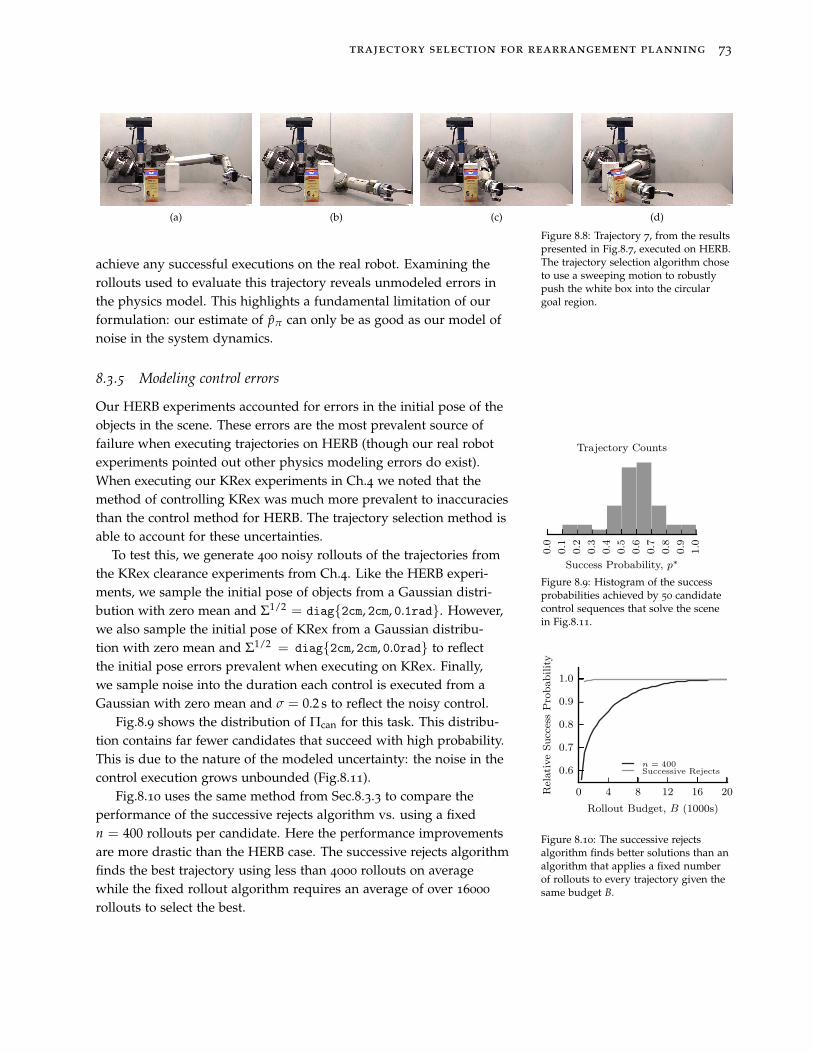
trajectory selection for rearrangement planning 73
(a) (b) (c) (d)
Figure 8.8: Trajectory 7, from the resultspresented in Fig.8.7, executed on HERB.The trajectory selection algorithm choseto use a sweeping motion to robustlypush the white box into the circulargoal region.
achieve any successful executions on the real robot. Examining therollouts used to evaluate this trajectory reveals unmodeled errors inthe physics model. This highlights a fundamental limitation of ourformulation: our estimate of pπ can only be as good as our model ofnoise in the system dynamics.
8.3.5 Modeling control errors
Our HERB experiments accounted for errors in the initial pose of theobjects in the scene. These errors are the most prevalent source offailure when executing trajectories on HERB (though our real robotexperiments pointed out other physics modeling errors do exist).When executing our KRex experiments in Ch.4 we noted that themethod of controlling KRex was much more prevalent to inaccuraciesthan the control method for HERB. The trajectory selection method isable to account for these uncertainties.
0.0
0.1
0.2
0.3
0.4
0.5
0.6
0.7
0.8
0.9
1.0
Success Probability, p∗
Trajectory Counts
Figure 8.9: Histogram of the successprobabilities achieved by 50 candidatecontrol sequences that solve the scenein Fig.8.11.
To test this, we generate 400 noisy rollouts of the trajectories fromthe KRex clearance experiments from Ch.4. Like the HERB experi-ments, we sample the initial pose of objects from a Gaussian distri-bution with zero mean and Σ1/2 = diag{2cm, 2cm, 0.1rad}. However,we also sample the initial pose of KRex from a Gaussian distribu-tion with zero mean and Σ1/2 = diag{2cm, 2cm, 0.0rad} to reflectthe initial pose errors prevalent when executing on KRex. Finally,we sample noise into the duration each control is executed from aGaussian with zero mean and σ = 0.2 s to reflect the noisy control.
Fig.8.9 shows the distribution of Πcan for this task. This distribu-tion contains far fewer candidates that succeed with high probability.This is due to the nature of the modeled uncertainty: the noise in thecontrol execution grows unbounded (Fig.8.11).
0 4 8 12 16 20
Rollout Budget, B (1000s)
0.6
0.7
0.8
0.9
1.0
RelativeSuccessProbability
n = 400Successive Rejects
Figure 8.10: The successive rejectsalgorithm finds better solutions than analgorithm that applies a fixed numberof rollouts to every trajectory given thesame budget B.
Fig.8.10 uses the same method from Sec.8.3.3 to compare theperformance of the successive rejects algorithm vs. using a fixedn = 400 rollouts per candidate. Here the performance improvementsare more drastic than the HERB case. The successive rejects algorithmfinds the best trajectory using less than 4000 rollouts on averagewhile the fixed rollout algorithm requires an average of over 16000
rollouts to select the best.
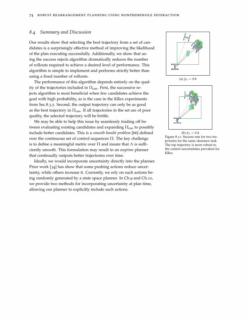
74 robust rearrangement planning using nonprehensile interaction
8.4 Summary and Discussion
Our results show that selecting the best trajectory from a set of can-didates is a surprisingly effective method of improving the likelihoodof the plan executing successfully. Additionally, we show that us-ing the success rejects algorithm dramatically reduces the numberof rollouts required to achieve a desired level of performance. Thisalgorithm is simple to implement and performs strictly better thanusing a fixed number of rollouts.
(a) pπ = 0.8
(b) pπ = 0.4Figure 8.11: Success rate for two tra-jectories for the same clearance task.The top trajectory is more robust tothe control uncertainties prevalent forKRex.
The performance of this algorithm depends entirely on the qual-ity of the trajectories included in Πcan. First, the successive re-jects algorithm is most beneficial when few candidates achieve thegoal with high probability, as is the case in the KRex experimentsfrom Sec.8.3.5. Second, the output trajectory can only be as goodas the best trajectory in Πcan. If all trajectories in the set are of poorquality, the selected trajectory will be brittle.
We may be able to help this issue by seamlessly trading off be-tween evaluating existing candidates and expanding Πcan to possiblyinclude better candidates. This is a smooth bandit problem [66] definedover the continuous set of control sequences Π. The key challengeis to define a meaningful metric over Π and insure that Λ is suffi-ciently smooth. This formulation may result in an anytime plannerthat continually outputs better trajectories over time.
Ideally, we would incorporate uncertainty directly into the planner.Prior work [34] has show that some pushing actions reduce uncer-tainty, while others increase it. Currently, we rely on such actions be-ing randomly generated by a state space planner. In Ch.9 and Ch.10,we provide two methods for incorporating uncertainty at plan time,allowing our planner to explicitly include such actions.
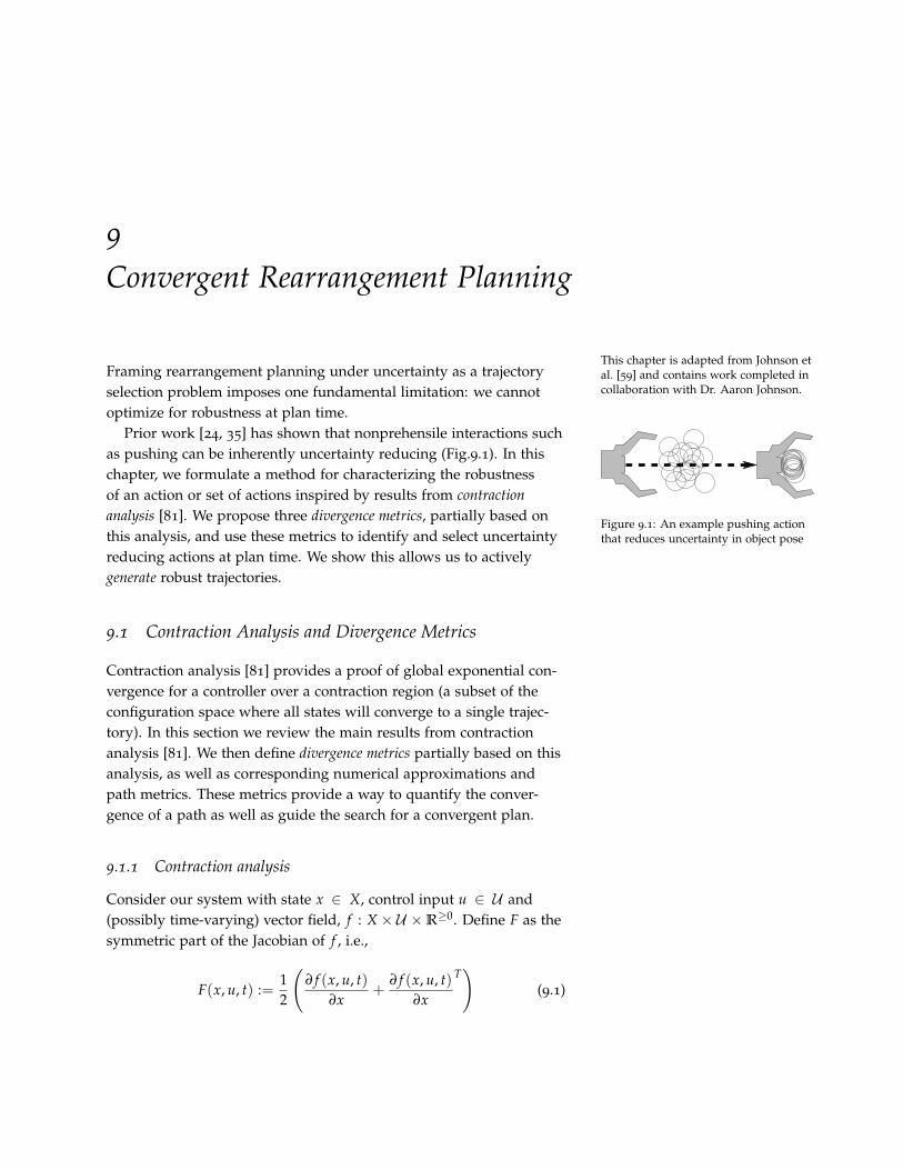
9
Convergent Rearrangement Planning
This chapter is adapted from Johnson etal. [59] and contains work completed incollaboration with Dr. Aaron Johnson.
Framing rearrangement planning under uncertainty as a trajectoryselection problem imposes one fundamental limitation: we cannotoptimize for robustness at plan time.
Figure 9.1: An example pushing actionthat reduces uncertainty in object pose
Prior work [24, 35] has shown that nonprehensile interactions suchas pushing can be inherently uncertainty reducing (Fig.9.1). In thischapter, we formulate a method for characterizing the robustnessof an action or set of actions inspired by results from contraction
analysis [81]. We propose three divergence metrics, partially based onthis analysis, and use these metrics to identify and select uncertaintyreducing actions at plan time. We show this allows us to activelygenerate robust trajectories.
9.1 Contraction Analysis and Divergence Metrics
Contraction analysis [81] provides a proof of global exponential con-vergence for a controller over a contraction region (a subset of theconfiguration space where all states will converge to a single trajec-tory). In this section we review the main results from contractionanalysis [81]. We then define divergence metrics partially based on thisanalysis, as well as corresponding numerical approximations andpath metrics. These metrics provide a way to quantify the conver-gence of a path as well as guide the search for a convergent plan.
9.1.1 Contraction analysis
Consider our system with state x ∈ X, control input u ∈ U and(possibly time-varying) vector field, f : X × U ×R
≥0. Define F as thesymmetric part of the Jacobian of f , i.e.,
F(x, u, t) :=12
(
∂ f (x, u, t)
∂x+
∂ f (x, u, t)
∂x
T)
(9.1)
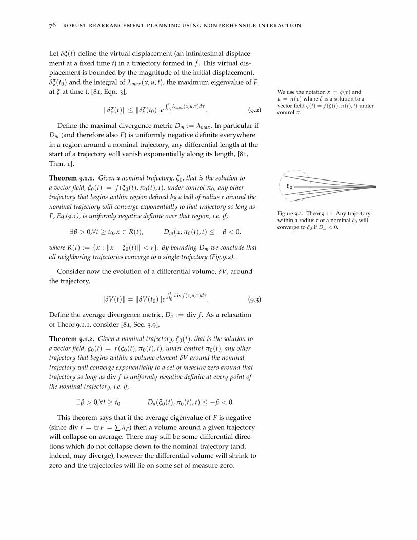
76 robust rearrangement planning using nonprehensile interaction
Let δξ(t) define the virtual displacement (an infinitesimal displace-ment at a fixed time t) in a trajectory formed in f . This virtual dis-placement is bounded by the magnitude of the initial displacement,δξ(t0) and the integral of λmax(x, u, t), the maximum eigenvalue of F
at ξ at time t, [81, Eqn. 3], We use the notation x = ξ(τ) andu = π(τ) where ξ is a solution to avector field ξ(t) = f (ξ(t), π(t), t) undercontrol π.‖δξ(t)‖ ≤ ‖δξ(t0)‖e
∫ tt0
λmax(x,u,τ)dτ. (9.2)
Define the maximal divergence metric Dm := λmax. In particular ifDm (and therefore also F) is uniformly negative definite everywherein a region around a nominal trajectory, any differential length at thestart of a trajectory will vanish exponentially along its length, [81,Thm. 1],
ξ0
Figure 9.2: Theor.9.1.1: Any trajectorywithin a radius r of a nominal ξ0 willconverge to ξ0 if Dm < 0.
Theorem 9.1.1. Given a nominal trajectory, ξ0, that is the solution to
a vector field, ξ0(t) = f (ξ0(t), π0(t), t), under control π0, any other
trajectory that begins within region defined by a ball of radius r around the
nominal trajectory will converge exponentially to that trajectory so long as
F, Eq.(9.1), is uniformly negative definite over that region, i.e. if,
∃β > 0,∀t ≥ t0, x ∈ R(t), Dm(x, π0(t), t) ≤ −β < 0,
where R(t) := {x : ‖x− ξ0(t)‖ < r}. By bounding Dm we conclude that
all neighboring trajectories converge to a single trajectory (Fig.9.2).
Consider now the evolution of a differential volume, δV, aroundthe trajectory,
‖δV(t)‖ = ‖δV(t0)‖e∫ t
t0div f (x,u,τ)dτ
. (9.3)
Define the average divergence metric, Da := div f . As a relaxationof Theor.9.1.1, consider [81, Sec. 3.9],
Theorem 9.1.2. Given a nominal trajectory, ξ0(t), that is the solution to
a vector field, ξ0(t) = f (ξ0(t), π0(t), t), under control π0(t), any other
trajectory that begins within a volume element δV around the nominal
trajectory will converge exponentially to a set of measure zero around that
trajectory so long as div f is uniformly negative definite at every point of
the nominal trajectory, i.e. if,
∃β > 0,∀t ≥ t0 Da(ξ0(t), π0(t), t) ≤ −β < 0.
This theorem says that if the average eigenvalue of F is negative(since div f = tr F = ∑ λF) then a volume around a given trajectorywill collapse on average. There may still be some differential direc-tions which do not collapse down to the nominal trajectory (and,indeed, may diverge), however the differential volume will shrink tozero and the trajectories will lie on some set of measure zero.
convergent rearrangement planning 77
Extending beyond the results of contraction analysis, consider theevolution of the expected value of a virtual displacement, E
[‖δξ(t)‖
],
taken over some distribution,
E[‖δξ(t)‖
]=E[‖δξ(t0)‖
]e∫ t
t0De(x,u,τ)dτ
, (9.4)
De(x, u, t) :=d
dtln E
[‖δξ(t)‖
]. (9.5)
This form of the expected divergence metric, De, may not seem par-ticularly useful. However we will show in the next section that it iseasy to compute numerically.
Dm Maximal divergenceDa Average divergenceDe Expected divergence
Table 9.1: Divergence metricsTab.9.1 lists the metrics presented in this section for easy referenceduring the remainder of this chapter.
9.1.2 Numerical approximation
The contraction analysis of [81] assumes a closed form differentiablevector field. In rearrangement planning, this vector field is defined bythe non-holonomic constraint (Eq.(2.1)) that describes the motion ofthe manipulator and objects. This vector field is not smooth – contactis inherently discontinuous – and lacks an analytic representation(although for simple problems this is theoretically possible [60]).We have shown that f can be effectively approximated by a physicssimulator, however analytic divergence measures cannot be derived.Instead, to approximate Dm, Da, and De we introduce numericaldivergence metrics that approximate the virtual displacement, δξ,with finite samples.
Given a nominal trajectory, ξ0(t), generated by applying some ac-tion π0(t) to a system with dynamics f , a perturbed trajectory (ornoisy rollout), ξi(t), is the solution to the same system and action asthe nominal trajectory, ξi(t) = f (ξi(t), π0(t), t), but with a differentinitial condition, ξi(t0) = ξ0(t0) + δξi. Thus Eq.(9.2) may be modi-fied as, Here x0 = ξ0(τ) and u0 = π0(τ).
‖ξi(t)− ξ0(t)‖ ≤ ‖ξi(t0)− ξ0(t0)‖e∫ t
t0Dm(x0,u0,τ)dτ
, (9.6)
which holds in the limit as δξi goes to zero. Thus if Dm < 0, the ratio,‖ξi(t) − ξ0(t)‖/‖ξi(t0) − ξ0(t0)‖, goes to zero exponentially. To getthe closest approximation, consider the largest such ratio, each ofwhich abides by the bound in Eq.(9.6),
maxi
‖ξi(t)− ξ0(t)‖
‖ξi(t0)− ξ0(t0)‖≤e
∫ tt0
Dm(x0,u0,τ)dτ(9.7)
For a small time step δt, we have that,
Dm(x0, u0, t) :=1δt
ln maxi
‖ξi(t + δt)− ξ0(t + δt)‖
‖ξi(t)− ξ0(t)‖(9.8)
78 robust rearrangement planning using nonprehensile interaction
and we arrive at the numerical approximation, Dm ≈ Dm.Similarly, for the average divergence Da, we will approximate
the differential volume by taking the volume spanned by a finiteset of points. Let V(ξ(t)) define such a volume, then Da ≈ Da is anumerical approximation where,
Da(x0, u0, t) :=1δt
lnV(ξ(t + δt))
V(ξ(t))(9.9)
Finally, to estimate the divergence of expectation De ≈ De, con-sider the ratio of the average displacements,
De(x0, u0, t) :=1δt
ln1N ∑
Ni=0 ‖ξi(t + δt)− ξ0(t + δt)‖
1N ∑
Ni=0 ‖ξi(t)− ξ0(t)‖
(9.10)
The approximation holds exactly in the limit as N goes to infinityand δt goes to zero, as can be derived from Eq.(9.10) or from stan-dard results in Monte Carlo estimation, e.g. [37, Sec. 1.3.1]. Note thatthe condition in Eq.(9.4) will hold over the length of a path if the setof noisy samples, {δξi}, is drawn once at time t0 and not indepen-dently at each time step.
9.1.3 Path metrics
Define for each metric Di the exponential of the integral of that met-ric along a trajectory,
Ei := e∫ T
0 Di(x,u,τ)dτ (9.11)
where note that some of the divergence metrics admit the followingsimplifications,
Ea = exp(∫ t
t0
div f (ξ(τ), π(τ), τ)dτ
)
=‖δV(ξ(t))‖
‖δV(ξ(t0))‖
Ea = exp
(
limδt→0
∑τ
lnV(ξ(τ + δt))
V(ξ(τ))
)
=V(ξ(t))
V(ξ(t0))
Ee = exp(∫ t
t0
d
dτln E
[‖δξ(τ)‖
]dτ
)
=E[‖δξ(t)‖
]
E[‖δξ(t0)‖
]
Ee = exp limδt→0
(t
∑τ=t0
ln1N ∑
Ni=0 ‖δξi(τ + δt)‖
1N ∑
Ni=0 ‖δξi(τ)‖
)
=1N ∑
Ni=0 ‖δξi(t)‖
1N ∑
Ni=0 ‖δξi(t0)‖
.
9.2 Planning with Divergence Metrics
The contraction analysis described in the previous section providesconditions for convergence but it does not provide a method of find-
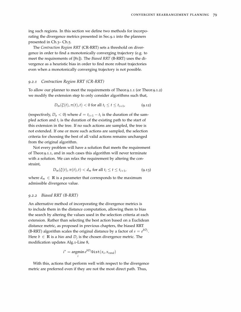
convergent rearrangement planning 79
ing such regions. In this section we define two methods for incorpo-rating the divergence metrics presented in Sec.9.1 into the plannerspresented in Ch.3– Ch.5.
The Contraction Region RRT (CR-RRT) sets a threshold on diver-gence in order to find a monotonically converging trajectory (e.g. tomeet the requirements of [81]). The Biased RRT (B-RRT) uses the di-vergence as a heuristic bias in order to find more robust trajectorieseven when a monotonically converging trajectory is not possible.
9.2.1 Contraction Region RRT (CR-RRT)
To allow our planner to meet the requirements of Theor.9.1.1 (or Theor.9.1.2)we modify the extension step to only consider algorithms such that,
Dm(ξ(t), π(t), t) < 0 for all ti ≤ t ≤ ti+1, (9.12)
(respectively, Da < 0) where d = ti+1 − ti is the duration of the sam-pled action and ti is the duration of the existing path to the start ofthis extension in the tree. If no such actions are sampled, the tree isnot extended. If one or more such actions are sampled, the selectioncriteria for choosing the best of all valid actions remains unchangedfrom the original algorithm.
Not every problem will have a solution that meets the requirementof Theor.9.1.1, and in such cases this algorithm will never terminatewith a solution. We can relax the requirement by altering the con-straint,
Dm(ξ(t), π(t), t) < dm for all ti ≤ t ≤ ti+1, (9.13)
where dm ∈ R is a parameter that corresponds to the maximumadmissible divergence value.
9.2.2 Biased RRT (B-RRT)
An alternative method of incorporating the divergence metrics isto include them in the distance computation, allowing them to biasthe search by altering the values used in the selection criteria at eachextension. Rather than selecting the best action based on a Euclideandistance metric, as proposed in previous chapters, the biased RRT(B-RRT) algorithm scales the original distance by a factor of s = ebDj .Here b ∈ R is a bias and Dj is the chosen divergence metric. Themodification updates Alg.1-Line 8,
i∗ = argmini
ebDjDist(xi, xrand)
With this, actions that perform well with respect to the divergencemetric are preferred even if they are not the most direct path. Thus,
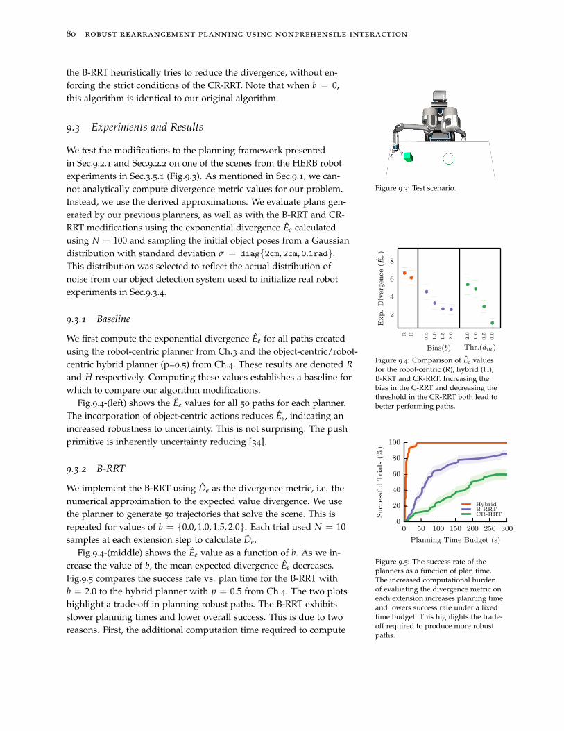
80 robust rearrangement planning using nonprehensile interaction
the B-RRT heuristically tries to reduce the divergence, without en-forcing the strict conditions of the CR-RRT. Note that when b = 0,this algorithm is identical to our original algorithm.
9.3 Experiments and Results
Figure 9.3: Test scenario.
We test the modifications to the planning framework presentedin Sec.9.2.1 and Sec.9.2.2 on one of the scenes from the HERB robotexperiments in Sec.3.5.1 (Fig.9.3). As mentioned in Sec.9.1, we can-not analytically compute divergence metric values for our problem.Instead, we use the derived approximations. We evaluate plans gen-erated by our previous planners, as well as with the B-RRT and CR-RRT modifications using the exponential divergence Ee calculatedusing N = 100 and sampling the initial object poses from a Gaussiandistribution with standard deviation σ = diag{2cm, 2cm, 0.1rad}.This distribution was selected to reflect the actual distribution ofnoise from our object detection system used to initialize real robotexperiments in Sec.9.3.4.
9.3.1 Baseline
R H
2
4
6
8
Exp.Divergen
ce( E
e)
0.5
1.0
1.5
2.0
Bias(b)
2.0
1.0
0.5
0.0
Thr.(dm)
Figure 9.4: Comparison of Ee valuesfor the robot-centric (R), hybrid (H),B-RRT and CR-RRT. Increasing thebias in the C-RRT and decreasing thethreshold in the CR-RRT both lead tobetter performing paths.
We first compute the exponential divergence Ee for all paths createdusing the robot-centric planner from Ch.3 and the object-centric/robot-centric hybrid planner (p=0.5) from Ch.4. These results are denoted R
and H respectively. Computing these values establishes a baseline forwhich to compare our algorithm modifications.
Fig.9.4-(left) shows the Ee values for all 50 paths for each planner.The incorporation of object-centric actions reduces Ee, indicating anincreased robustness to uncertainty. This is not surprising. The pushprimitive is inherently uncertainty reducing [34].
9.3.2 B-RRT
We implement the B-RRT using De as the divergence metric, i.e. thenumerical approximation to the expected value divergence. We usethe planner to generate 50 trajectories that solve the scene. This isrepeated for values of b = {0.0, 1.0, 1.5, 2.0}. Each trial used N = 10samples at each extension step to calculate De.
0 50 100 150 200 250 300
Planning Time Budget (s)
0
20
40
60
80
100
SuccessfulTrials
(%)
HybridB-RRTCR-RRT
Figure 9.5: The success rate of theplanners as a function of plan time.The increased computational burdenof evaluating the divergence metric oneach extension increases planning timeand lowers success rate under a fixedtime budget. This highlights the trade-off required to produce more robustpaths.
Fig.9.4-(middle) shows the Ee value as a function of b. As we in-crease the value of b, the mean expected divergence Ee decreases.Fig.9.5 compares the success rate vs. plan time for the B-RRT withb = 2.0 to the hybrid planner with p = 0.5 from Ch.4. The two plotshighlight a trade-off in planning robust paths. The B-RRT exhibitsslower planning times and lower overall success. This is due to tworeasons. First, the additional computation time required to compute
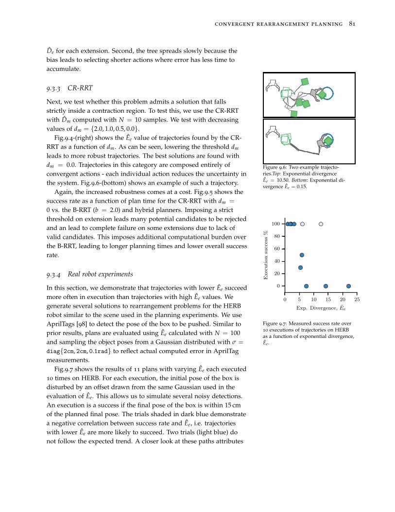
convergent rearrangement planning 81
De for each extension. Second, the tree spreads slowly because thebias leads to selecting shorter actions where error has less time toaccumulate.
9.3.3 CR-RRT
Next, we test whether this problem admits a solution that fallsstrictly inside a contraction region. To test this, we use the CR-RRTwith Dm computed with N = 10 samples. We test with decreasingvalues of dm = {2.0, 1.0, 0.5, 0.0}.
Figure 9.6: Two example trajecto-ries.Top: Exponential divergenceEe = 10.50. Bottom: Exponential di-vergence Ee = 0.15.
Fig.9.4-(right) shows the Ee value of trajectories found by the CR-RRT as a function of dm. As can be seen, lowering the threshold dm
leads to more robust trajectories. The best solutions are found withdm = 0.0. Trajectories in this category are composed entirely ofconvergent actions - each individual action reduces the uncertainty inthe system. Fig.9.6-(bottom) shows an example of such a trajectory.
Again, the increased robustness comes at a cost. Fig.9.5 shows thesuccess rate as a function of plan time for the CR-RRT with dm =
0 vs. the B-RRT (b = 2.0) and hybrid planners. Imposing a strictthreshold on extension leads many potential candidates to be rejectedand an lead to complete failure on some extensions due to lack ofvalid candidates. This imposes additional computational burden overthe B-RRT, leading to longer planning times and lower overall successrate.
9.3.4 Real robot experiments
0 5 10 15 20 25
Exp. Divergence, Ee
0
20
40
60
80
100
Executionsu
ccess%
Figure 9.7: Measured success rate over10 executions of trajectories on HERBas a function of exponential divergence,Ee.
In this section, we demonstrate that trajectories with lower Ee succeedmore often in execution than trajectories with high Ee values. Wegenerate several solutions to rearrangement problems for the HERBrobot similar to the scene used in the planning experiments. We useAprilTags [98] to detect the pose of the box to be pushed. Similar toprior results, plans are evaluated using Ee calculated with N = 100and sampling the object poses from a Gaussian distributed with σ =
diag{2cm, 2cm, 0.1rad} to reflect actual computed error in AprilTagmeasurements.
Fig.9.7 shows the results of 11 plans with varying Ee each executed10 times on HERB. For each execution, the initial pose of the box isdisturbed by an offset drawn from the same Gaussian used in theevaluation of Ee. This allows us to simulate several noisy detections.An execution is a success if the final pose of the box is within 15 cmof the planned final pose. The trials shaded in dark blue demonstratea negative correlation between success rate and Ee, i.e. trajectorieswith lower Ee are more likely to succeed. Two trials (light blue) donot follow the expected trend. A closer look at these paths attributes
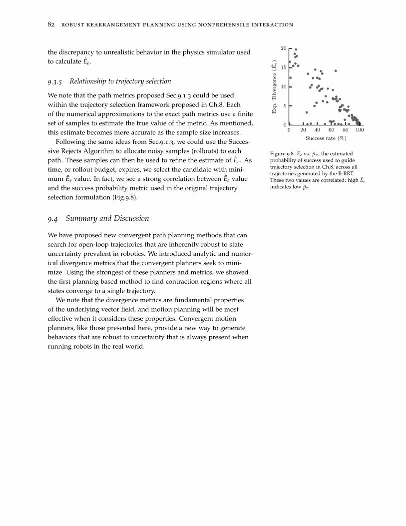
82 robust rearrangement planning using nonprehensile interaction
the discrepancy to unrealistic behavior in the physics simulator usedto calculate Ee.
9.3.5 Relationship to trajectory selection
0 20 40 60 80 100
Success rate (%)
0
5
10
15
20
Exp.Divergen
ce( E
e)
Figure 9.8: Ee vs. pπ , the estimatedprobability of success used to guidetrajectory selection in Ch.8, across alltrajectories generated by the B-RRT.These two values are correlated: high Ee
indicates low pπ .
We note that the path metrics proposed Sec.9.1.3 could be usedwithin the trajectory selection framework proposed in Ch.8. Eachof the numerical approximations to the exact path metrics use a finiteset of samples to estimate the true value of the metric. As mentioned,this estimate becomes more accurate as the sample size increases.
Following the same ideas from Sec.9.1.3, we could use the Succes-sive Rejects Algorithm to allocate noisy samples (rollouts) to eachpath. These samples can then be used to refine the estimate of Ee. Astime, or rollout budget, expires, we select the candidate with mini-mum Ee value. In fact, we see a strong correlation between Ee valueand the success probability metric used in the original trajectoryselection formulation (Fig.9.8).
9.4 Summary and Discussion
We have proposed new convergent path planning methods that cansearch for open-loop trajectories that are inherently robust to stateuncertainty prevalent in robotics. We introduced analytic and numer-ical divergence metrics that the convergent planners seek to mini-mize. Using the strongest of these planners and metrics, we showedthe first planning based method to find contraction regions where allstates converge to a single trajectory.
We note that the divergence metrics are fundamental propertiesof the underlying vector field, and motion planning will be mosteffective when it considers these properties. Convergent motionplanners, like those presented here, provide a new way to generatebehaviors that are robust to uncertainty that is always present whenrunning robots in the real world.
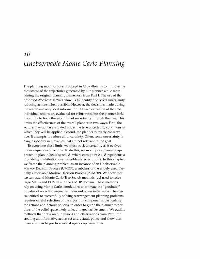
10
Unobservable Monte Carlo Planning
The planning modifications proposed in Ch.9 allow us to improve therobustness of the trajectories generated by our planner while main-taining the original planning framework from Part I. The use of theproposed divergence metrics allow us to identify and select uncertaintyreducing actions when possible. However, the decisions made duringthe search use only local information. At each extension of the tree,individual actions are evaluated for robustness, but the planner lacksthe ability to track the evolution of uncertainty through the tree. Thislimits the effectiveness of the overall planner in two ways. First, theactions may not be evaluated under the true uncertainty conditions inwhich they will be applied. Second, the planner is overly conserva-tive. It attempts to reduce all uncertainty. Often, some uncertainty isokay, especially in movables that are not relevant to the goal.
To overcome these limits we must track uncertainty as it evolvesunder sequences of actions. To do this, we modify our planning ap-proach to plan in belief space, B, where each point b ∈ B represents aprobability distribution over possible states, b = p(x). In this chapter,we frame the planning problem as an instance of an UnobservableMarkov Decision Process (UMDP), a subclass of the widely used Par-tially Observable Markov Decision Process (POMDP). We show thatwe can extend Monte Carlo Tree Search methods [25] used to solvelarge MDPs and POMDPs to the UMDP domain. These methodsrely on using Monte Carlo simulations to estimate the “goodness”or value of an action sequence under unknown initial state. The con-
tact critical to successfully solving rearrangement planning problemsrequires careful selection of the algorithm components, particularlythe actions and default policies, in order to guide the planner to por-tions of the belief space likely to lead to goal achievement. We outlinemethods that draw on our lessons and observations from Part I forcreating an informative action set and default policy and show thatthese allow us to produce robust open-loop trajectories.
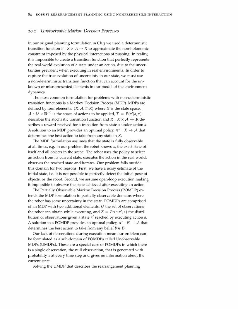
84 robust rearrangement planning using nonprehensile interaction
10.1 Unobservable Markov Decision Processes
In our original planning formulation in Ch.3 we used a deterministictransition function Γ : X ×A → X to approximate the non-holonomicconstraint imposed by the physical interactions of pushing. In reality,it is impossible to create a transition function that perfectly representsthe real-world evolution of a state under an action, due to the uncer-tainties prevalent when executing in real environments. In order tocapture the true evolution of uncertainty in our state, we must usea non-deterministic transition function that can account for the un-known or misrepresented elements in our model of the environmentdynamics.
The most common formulation for problems with non-deterministictransition functions is a Markov Decision Process (MDP). MDPs aredefined by four elements: 〈X,A, T, R〉 where X is the state space,A : U × R
≥0 is the space of actions to be applied, T = P(x′|a, x)
describes the stochastic transition function and R : X ×A → R de-scribes a reward received for a transition from state x under action a.A solution to an MDP provides an optimal policy, π∗ : X → A thatdetermines the best action to take from any state in X.
The MDP formulation assumes that the state is fully observableat all times, e.g. in our problem the robot knows x, the exact state ofitself and all objects in the scene. The robot uses the policy to selectan action from its current state, executes the action in the real world,observes the reached state and iterates. Our problem falls outsidethis domain for two reasons. First, we have a noisy estimate of theinitial state, i.e. it is not possible to perfectly detect the initial pose ofobjects, or the robot. Second, we assume open-loop execution makingit impossible to observe the state achieved after executing an action.
The Partially Observable Markov Decision Process (POMDP) ex-tends the MDP formulation to partially observable domains wherethe robot has some uncertainty in the state. POMDPs are comprisedof an MDP with two additional elements: O the set of observationsthe robot can obtain while executing, and Z = Pr(o|x′, a) the distri-bution of observations given a state x′ reached by executing action a.A solution to a POMDP provides an optimal policy, π∗ : B → A thatdetermines the best action to take from any belief b ∈ B.
Our lack of observations during execution mean our problem canbe formulated as a sub-domain of POMDPs called UnobservableMDPs (UMDPs). These are a special case of POMDPs in which thereis a single observation, the null observation, that is generated withprobability 1 at every time step and gives no information about thecurrent state.
Solving the UMDP that describes the rearrangement planning
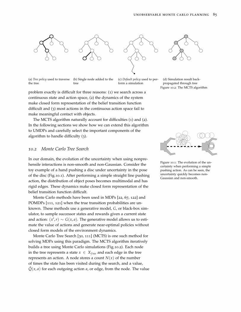
unobservable monte carlo planning 85
(a) Tree policy used to traversethe tree
(b) Single node added to thetree
(c) Default policy used to per-form a simulation
(d) Simulation result back-propagated through tree
Figure 10.2: The MCTS algorithm
problem exactly is difficult for three reasons: (1) we search across acontinuous state and action space, (2) the dynamics of the systemmake closed form representation of the belief transition functiondifficult and (3) most actions in the continuous action space fail tomake meaningful contact with objects.
The MCTS algorithm naturally account for difficulties (1) and (2).In the following sections we show how we can extend this algorithmto UMDPs and carefully select the important components of thealgorithm to handle difficulty (3).
10.2 Monte Carlo Tree Search
Figure 10.1: The evolution of the un-certainty when performing a simplepushing action. As can be seen, theuncertainty quickly becomes non-Gaussian and non-smooth.
In our domain, the evolution of the uncertainty when using nonpre-hensile interactions is non-smooth and non-Gaussian. Consider thetoy example of a hand pushing a disc under uncertainty in the poseof the disc (Fig.10.1). After performing a simple straight line pushingaction, the distribution of object poses becomes multimodal and hasrigid edges. These dynamics make closed form representation of thebelief transition function difficult.
Monte Carlo methods have been used in MDPs [22, 67, 122] andPOMDPs [111, 121] when the true transition probabilities are un-known. These methods use a generative model, G, or black-box sim-ulator, to sample successor states and rewards given a current stateand action: (x′, r) ∼ G(x, a). The generative model allows us to esti-mate the value of actions and generate near-optimal policies withoutclosed form models of the environment dynamics.
Monte Carlo Tree Search [30, 111] (MCTS) is one such method forsolving MDPs using this paradigm. The MCTS algorithm iterativelybuilds a tree using Monte Carlo simulations (Fig.10.2). Each nodein the tree represents a state x ∈ X f ree and each edge in the treerepresents an action. A node stores a count N(x) of the numberof times the state has been visited during the search, and a value,Q(x, a) for each outgoing action a, or edge, from the node. The value
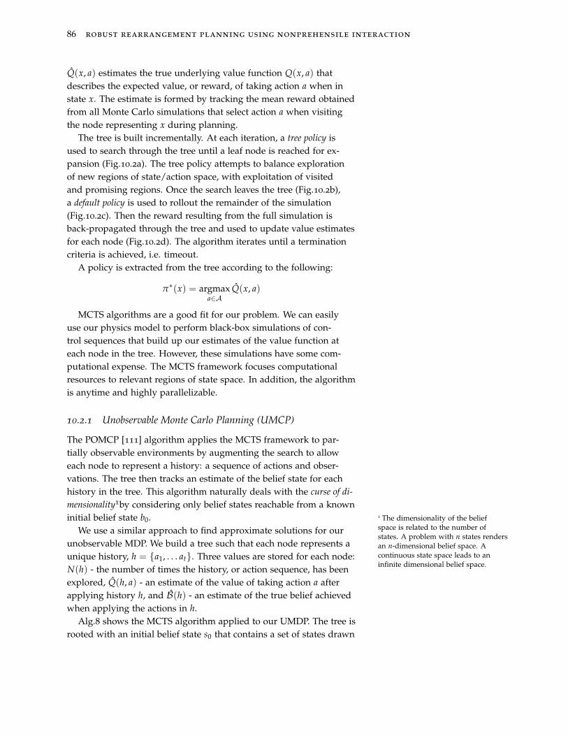
86 robust rearrangement planning using nonprehensile interaction
Q(x, a) estimates the true underlying value function Q(x, a) thatdescribes the expected value, or reward, of taking action a when instate x. The estimate is formed by tracking the mean reward obtainedfrom all Monte Carlo simulations that select action a when visitingthe node representing x during planning.
The tree is built incrementally. At each iteration, a tree policy isused to search through the tree until a leaf node is reached for ex-pansion (Fig.10.2a). The tree policy attempts to balance explorationof new regions of state/action space, with exploitation of visitedand promising regions. Once the search leaves the tree (Fig.10.2b),a default policy is used to rollout the remainder of the simulation(Fig.10.2c). Then the reward resulting from the full simulation isback-propagated through the tree and used to update value estimatesfor each node (Fig.10.2d). The algorithm iterates until a terminationcriteria is achieved, i.e. timeout.
A policy is extracted from the tree according to the following:
π∗(x) = argmaxa∈A
Q(x, a)
MCTS algorithms are a good fit for our problem. We can easilyuse our physics model to perform black-box simulations of con-trol sequences that build up our estimates of the value function ateach node in the tree. However, these simulations have some com-putational expense. The MCTS framework focuses computationalresources to relevant regions of state space. In addition, the algorithmis anytime and highly parallelizable.
10.2.1 Unobservable Monte Carlo Planning (UMCP)
The POMCP [111] algorithm applies the MCTS framework to par-tially observable environments by augmenting the search to alloweach node to represent a history: a sequence of actions and obser-vations. The tree then tracks an estimate of the belief state for eachhistory in the tree. This algorithm naturally deals with the curse of di-
mensionality1by considering only belief states reachable from a knowninitial belief state b0. 1 The dimensionality of the belief
space is related to the number ofstates. A problem with n states rendersan n-dimensional belief space. Acontinuous state space leads to aninfinite dimensional belief space.
We use a similar approach to find approximate solutions for ourunobservable MDP. We build a tree such that each node represents aunique history, h = {a1, . . . at}. Three values are stored for each node:N(h) - the number of times the history, or action sequence, has beenexplored, Q(h, a) - an estimate of the value of taking action a afterapplying history h, and B(h) - an estimate of the true belief achievedwhen applying the actions in h.
Alg.8 shows the MCTS algorithm applied to our UMDP. The tree isrooted with an initial belief state s0 that contains a set of states drawn
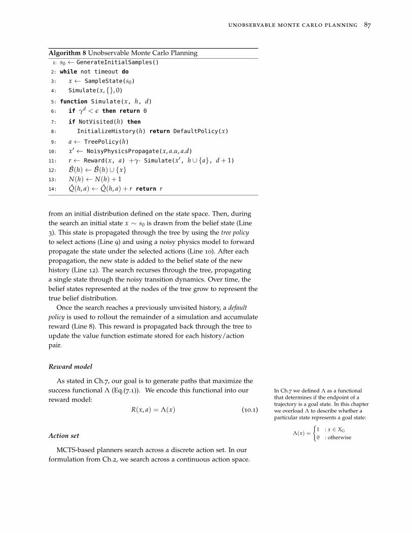
unobservable monte carlo planning 87
Algorithm 8 Unobservable Monte Carlo Planning1: s0 ← GenerateInitialSamples()
2: while not timeout do
3: x ← SampleState(s0)
4: Simulate(x, {}, 0)
5: function Simulate(x, h, d)
6: if γd< ǫ then return 0
7: if NotVisited(h) then
8: InitializeHistory(h) return DefaultPolicy(x)
9: a← TreePolicy(h)
10: x′ ← NoisyPhysicsPropagate(x, a.u, a.d)11: r ← Reward(x, a) +γ· Simulate(x′, h ∪ {a}, d + 1)12: B(h)← B(h) ∪ {x}
13: N(h)← N(h) + 114: Q(h, a)← Q(h, a) + r return r
from an initial distribution defined on the state space. Then, duringthe search an initial state x ∼ s0 is drawn from the belief state (Line3). This state is propagated through the tree by using the tree policy
to select actions (Line 9) and using a noisy physics model to forwardpropagate the state under the selected actions (Line 10). After eachpropagation, the new state is added to the belief state of the newhistory (Line 12). The search recurses through the tree, propagatinga single state through the noisy transition dynamics. Over time, thebelief states represented at the nodes of the tree grow to represent thetrue belief distribution.
Once the search reaches a previously unvisited history, a default
policy is used to rollout the remainder of a simulation and accumulatereward (Line 8). This reward is propagated back through the tree toupdate the value function estimate stored for each history/actionpair.
Reward model
As stated in Ch.7, our goal is to generate paths that maximize thesuccess functional Λ (Eq.(7.1)). We encode this functional into our In Ch.7 we defined Λ as a functional
that determines if the endpoint of atrajectory is a goal state. In this chapterwe overload Λ to describe whether aparticular state represents a goal state:
Λ(x) =
{
1 : x ∈ XG
0 : otherwise
reward model:R(x, a) = Λ(x) (10.1)
Action set
MCTS-based planners search across a discrete action set. In ourformulation from Ch.2, we search across a continuous action space.
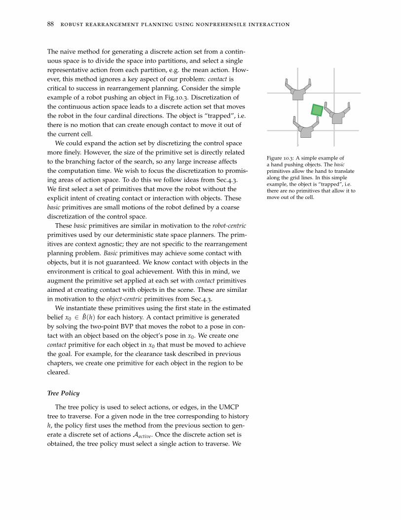
88 robust rearrangement planning using nonprehensile interaction
The naive method for generating a discrete action set from a contin-uous space is to divide the space into partitions, and select a singlerepresentative action from each partition, e.g. the mean action. How-ever, this method ignores a key aspect of our problem: contact iscritical to success in rearrangement planning. Consider the simpleexample of a robot pushing an object in Fig.10.3. Discretization ofthe continuous action space leads to a discrete action set that movesthe robot in the four cardinal directions. The object is “trapped”, i.e.there is no motion that can create enough contact to move it out ofthe current cell.
Figure 10.3: A simple example ofa hand pushing objects. The basicprimitives allow the hand to translatealong the grid lines. In this simpleexample, the object is “trapped”, i.e.there are no primitives that allow it tomove out of the cell.
We could expand the action set by discretizing the control spacemore finely. However, the size of the primitive set is directly relatedto the branching factor of the search, so any large increase affectsthe computation time. We wish to focus the discretization to promis-ing areas of action space. To do this we follow ideas from Sec.4.3.We first select a set of primitives that move the robot without theexplicit intent of creating contact or interaction with objects. Thesebasic primitives are small motions of the robot defined by a coarsediscretization of the control space.
These basic primitives are similar in motivation to the robot-centric
primitives used by our deterministic state space planners. The prim-itives are context agnostic; they are not specific to the rearrangementplanning problem. Basic primitives may achieve some contact withobjects, but it is not guaranteed. We know contact with objects in theenvironment is critical to goal achievement. With this in mind, weaugment the primitive set applied at each set with contact primitivesaimed at creating contact with objects in the scene. These are similarin motivation to the object-centric primitives from Sec.4.3.
We instantiate these primitives using the first state in the estimatedbelief x0 ∈ B(h) for each history. A contact primitive is generatedby solving the two-point BVP that moves the robot to a pose in con-tact with an object based on the object’s pose in x0. We create onecontact primitive for each object in x0 that must be moved to achievethe goal. For example, for the clearance task described in previouschapters, we create one primitive for each object in the region to becleared.
Tree Policy
The tree policy is used to select actions, or edges, in the UMCPtree to traverse. For a given node in the tree corresponding to historyh, the policy first uses the method from the previous section to gen-erate a discrete set of actions Aactive. Once the discrete action set isobtained, the tree policy must select a single action to traverse. We
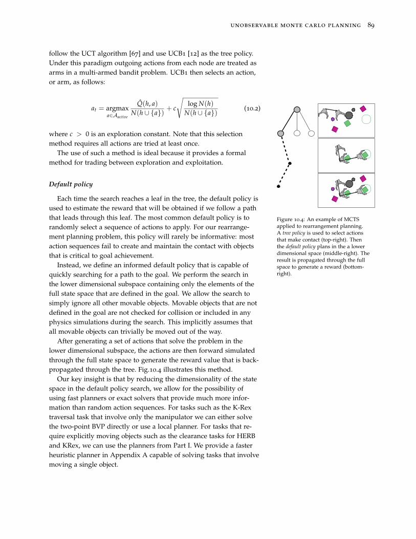
unobservable monte carlo planning 89
follow the UCT algorithm [67] and use UCB1 [12] as the tree policy.Under this paradigm outgoing actions from each node are treated asarms in a multi-armed bandit problem. UCB1 then selects an action,or arm, as follows:
at = argmaxa∈Aactive
Q(h, a)
N(h ∪ {a})+ c
√
log N(h)
N(h ∪ {a})(10.2)
where c > 0 is an exploration constant. Note that this selectionmethod requires all actions are tried at least once.
The use of such a method is ideal because it provides a formalmethod for trading between exploration and exploitation.
Default policy
Figure 10.4: An example of MCTSapplied to rearrangement planning.A tree policy is used to select actionsthat make contact (top-right). Thenthe default policy plans in the a lowerdimensional space (middle-right). Theresult is propagated through the fullspace to generate a reward (bottom-right).
Each time the search reaches a leaf in the tree, the default policy isused to estimate the reward that will be obtained if we follow a paththat leads through this leaf. The most common default policy is torandomly select a sequence of actions to apply. For our rearrange-ment planning problem, this policy will rarely be informative: mostaction sequences fail to create and maintain the contact with objectsthat is critical to goal achievement.
Instead, we define an informed default policy that is capable ofquickly searching for a path to the goal. We perform the search inthe lower dimensional subspace containing only the elements of thefull state space that are defined in the goal. We allow the search tosimply ignore all other movable objects. Movable objects that are notdefined in the goal are not checked for collision or included in anyphysics simulations during the search. This implicitly assumes thatall movable objects can trivially be moved out of the way.
After generating a set of actions that solve the problem in thelower dimensional subspace, the actions are then forward simulatedthrough the full state space to generate the reward value that is back-propagated through the tree. Fig.10.4 illustrates this method.
Our key insight is that by reducing the dimensionality of the statespace in the default policy search, we allow for the possibility ofusing fast planners or exact solvers that provide much more infor-mation than random action sequences. For tasks such as the K-Rextraversal task that involve only the manipulator we can either solvethe two-point BVP directly or use a local planner. For tasks that re-quire explicitly moving objects such as the clearance tasks for HERBand KRex, we can use the planners from Part I. We provide a fasterheuristic planner in Appendix A capable of solving tasks that involvemoving a single object.

90 robust rearrangement planning using nonprehensile interaction
Path extraction
We use our tree to create an anytime algorithm for extractingpaths. Upon request, a path π is extracted from the tree as follows.First, we extract πtree by repeatedly picking the action at such that:
at = argmaxa∈Aactive
Q(h, a)
Once a leaf is encountered, we query the belief represented by thehistory B(h) to obtain a probability of success pπtree = ∑x∈B(h) Λ(x).If this probability is lower than a threshold pgoal , we randomly selecta state from the belief x ∈ B(h) and use the default policy to generatea path πde f from x to the goal. If successful, all remaining samplesin B(h) are forward propagated through this path to get an updatedprobability of success pπ of the combined path π = πtree + πde f
formed from appending πde f to πtree. If pπ is better than the successprobability from previous requests, the path is returned. Otherwise,the previous best path is returned.
The use of a planner to generate the default policy means we canoften find paths that achieve the goal with non-zero probability. Ourinsight is that these path segments can be particularly useful whenthere is not enough planning time to deeply grow the tree.
10.3 Experiments and Results
We test the capabilities of the UMCP algorithm using the task ofHERB pushing an object to a goal region through clutter from Sec.3.5.1.We test three hypothesis:
H.1 The planner using the planned default policy allows us togenerate paths with higher probability of success than the plannerwith a random default policy.
H.2 Using explicit contact primitives allows the planner to gen-erate paths with high probability than a planner that uses a basic
action set formed by discretization of each dimension of the actionset.
H.3 Our UMCP planner that uses contact primitives and theplanned default policy is able to produce paths that exhibit higherprobability of success compared to anytime versions of baselineplanners presented in previous chapters.
unobservable monte carlo planning 91
H.1 verifies our intuition that using a powerful default policy ca-pable of explicitly attempting to achieve the goal will outperformthe common default policy that selects random action sequences,despite the extra resources and slower tree growth that result fromusing a planner to compute the default policy. H.2 tests the needfor primitives that explicitly try to create contact with goal criticalobjects. Finally, H.3 verifies the need to track the evolution of uncer-tainty through sequences of actions. We expect this to be especiallyimportant on problems where it is difficult to find sequences solelycomprised of uncertainty reducing actions, as preferred by the C-RRT.
In the following sections we detail our planning setup and provideresults for each hypothesis.
10.3.1 Test setup
We use the heuristic structured search planner from Appendix Aas the planned default policy. Specifically, we use the action set andheuristics described in the appendix in a weighted A* search withw = 5. This strongly biases our search toward the goal. We allow theplanner 1 s to find a path.
We run each version of the UMCP planner 50 times on a low clut-ter scene (Fig.10.6) and a high clutter scene (Fig.10.10). In each scene,we generate the initial belief s0 by sampling noise into the initialpose of each object from a Gaussian with distribution µ = 0, Σ1/2 =
diag{2cm, 2cm, 0.1rad}. We allow the UMCP planner to run for 300 s.We request and record a path every 15 s.
10.3.2 Baseline planners
We compare the estimated success rate of the paths generated by theUMCP algorithm to anytime versions of the B-RRT planner (withbias b = 2.0) from Ch.9 and the original PCRRT from Ch.3. To createanytime versions of these planners, we make as many repeated callsto the planner as possible within 300 s. When a call completes weperform a set of 100 noisy rollouts on the resulting control sequenceπ to generate an estimate pπ of the probability of success. We gen-erate these noisy rollouts using the same noise parameters used tocreate the initial belief s0 in the UMCP planner. We keep π only if ithas higher estimated success probability than all previous paths gen-erated by the planner. This is a similar algorithm to the AMD-RRTdescribed in [59] though we use probability of success rather thanperformance of the path under a divergence metric.
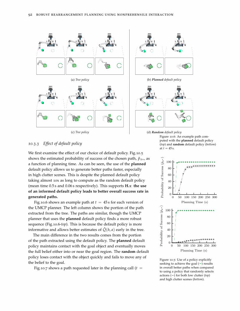
92 robust rearrangement planning using nonprehensile interaction
(a) Tree policy (b) Planned default policy
(c) Tree policy (d) Random default policy
Figure 10.6: An example path com-puted with the planned default policy(top) and random default policy (bottom)at t = 45 s.
10.3.3 Effect of default policy
We first examine the effect of our choice of default policy. Fig.10.5shows the estimated probability of success of the chosen path, pπ∗, asa function of planning time. As can be seen, the use of the planned
default policy allows us to generate better paths faster, especiallyin high clutter scenes. This is despite the planned default policytaking almost 10x as long to compute as the random default policy(mean time 0.5 s and 0.06 s respectively). This supports H.1: the use
of an informed default policy leads to better overall success rate in
generated paths. 0 50 100 150 200 250 300
Planning Time (s)
0
20
40
60
80
100ProbabilityofSuccess(p
π∗)
0 50 100 150 200 250 300
Planning Time (s)
0
20
40
60
80
100
ProbabilityofSuccess(p
π∗)
Figure 10.5: Use of a policy explicitlyseeking to achieve the goal ( ) resultsin overall better paths when comparedto using a policy that randomly selectsactions ( ) for both low clutter (top)and high clutter scenes (bottom).
Fig.10.6 shows an example path at t = 45 s for each version ofthe UMCP planner. The left column shows the portion of the pathextracted from the tree. The paths are similar, though the UMCPplanner that uses the planned default policy finds a more robustsequence (Fig.10.6-top). This is because the default policy is moreinformative and allows better estimates of Q(h, a) early in the tree.
The main difference in the two results comes from the portionof the path extracted using the default policy. The planned defaultpolicy maintains contact with the goal object and eventually movesthe full belief either into or near the goal region. The random defaultpolicy loses contact with the object quickly and fails to move any ofthe belief to the goal.
Fig.10.7 shows a path requested later in the planning call (t =
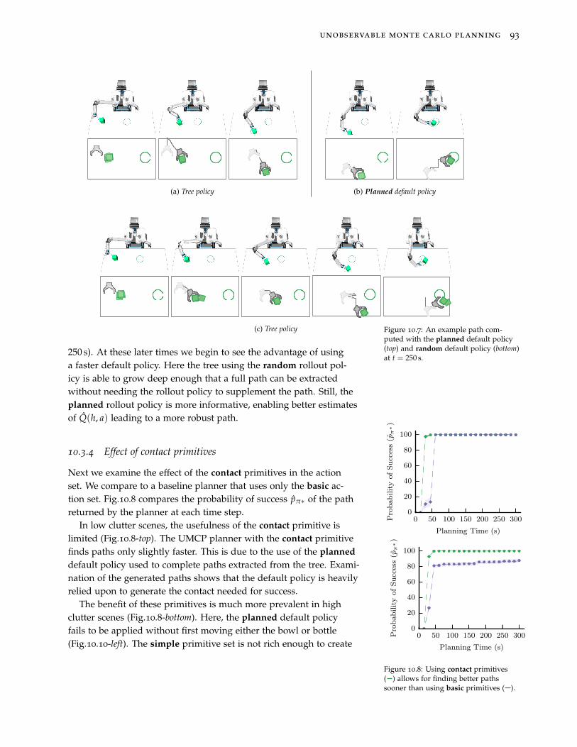
unobservable monte carlo planning 93
(a) Tree policy (b) Planned default policy
(c) Tree policy Figure 10.7: An example path com-puted with the planned default policy(top) and random default policy (bottom)at t = 250 s.
250 s). At these later times we begin to see the advantage of usinga faster default policy. Here the tree using the random rollout pol-icy is able to grow deep enough that a full path can be extractedwithout needing the rollout policy to supplement the path. Still, theplanned rollout policy is more informative, enabling better estimatesof Q(h, a) leading to a more robust path.
10.3.4 Effect of contact primitives
0 50 100 150 200 250 300
Planning Time (s)
0
20
40
60
80
100
ProbabilityofSuccess(p
π∗)
0 50 100 150 200 250 300
Planning Time (s)
0
20
40
60
80
100
ProbabilityofSuccess(p
π∗)
Figure 10.8: Using contact primitives( ) allows for finding better pathssooner than using basic primitives ( ).
Next we examine the effect of the contact primitives in the actionset. We compare to a baseline planner that uses only the basic ac-tion set. Fig.10.8 compares the probability of success pπ∗ of the pathreturned by the planner at each time step.
In low clutter scenes, the usefulness of the contact primitive islimited (Fig.10.8-top). The UMCP planner with the contact primitivefinds paths only slightly faster. This is due to the use of the planned
default policy used to complete paths extracted from the tree. Exami-nation of the generated paths shows that the default policy is heavilyrelied upon to generate the contact needed for success.
The benefit of these primitives is much more prevalent in highclutter scenes (Fig.10.8-bottom). Here, the planned default policyfails to be applied without first moving either the bowl or bottle(Fig.10.10-left). The simple primitive set is not rich enough to create

94 robust rearrangement planning using nonprehensile interaction
(a) Tree policy (b) Planned rollout policy
Figure 10.10: In high clutter scenes,the UMCP algorithm with contact
primitives performs well. The algorithmallows for increasing uncertainty in thepose of the bowl, as long as it does notinhibit goal achievement.
useful contact. In contrast, the contact primitive easily moves bothobjects out of the way in order to make contact with the box. Thenthe planned default policy can be applied to achieve the goal. Fig.10.10
depicts an example path found by the UMCP planner with contact
primitives.
10.3.5 Comparison to baseline planners
0 50 100 150 200 250 300
Planning Time (s)
0
20
40
60
80
100
ProbabilityofSuccess(p
π∗)
0 50 100 150 200 250 300
Planning Time (s)
0
20
40
60
80
100
ProbabilityofSuccess(p
π∗)
Figure 10.9: On simple scenes (top),the B-RRT from Ch.9 ( ) is able tofind better paths quickly. The UMCPalgorithm ( ) is able to find betterpaths more quickly than the PCRRTfrom Ch.3 ( ). On difficult scenes(bottom), the UMCP outperforms boththe C-RRT and the PCRRT.
Finally, we compare the UMCP planner using contact primitives inthe action set and the planned rollout policy to the baseline plannersdescribed in Sec.10.3.2. Fig.10.8 shows the estimated probability ofsuccess pπ∗ of each planner as a function of planning time.
For the low clutter scene the PCRRT and B-RRT are easily ableto find solutions (Fig.10.9-top). The B-RRT performs exceptionallywell here because there exists a solution comprised almost entirely ofuncertainty reducing, or low divergence, actions.
The advantage of the UMCP algorithm can be seen for the highclutter scene (Fig.10.9-bottom). Here, the B-RRT performs poorly be-cause the actions that reduce uncertainty in the goal object increaseuncertainty of the pose of other objects, such as the bottle or bowl(Fig.10.10). Such actions perform poorly under the divergence met-rics. As a result, the B-RRT is slow to explore and find solutions. TheUMCP allows for increasing uncertainty along dimensions that arenot important for goal achievement. This allows the planner to findsolutions more easily.
Overall, for planning time budgets greater than 30 s the UMCP al-gorithm finds solutions as good as the solutions found by the B-RRTand PCRRT algorithms in the low clutter scene. The UMCP algorithmoutperforms both baseline planners in the high clutter scene. Thispartially confirms H.3: Our UMCP planner that uses contact prim-
itives and the planned default policy is able to produce paths that
exhibit higher probability of success compared to anytime versions
of baseline planners presented in previous chapters.
unobservable monte carlo planning 95
10.4 Summary and Discussion
In this chapter we present Unobservable Monte Carlo Planning, analgorithm that extends MCTS to the Unobservable MDP domain. Weshow that by carefully selecting an informative default policy andan action set capable of generating contact with important objects inthe scene, we are able to plan solutions that are robust to uncertainty.The result is an anytime algorithm that returns good solutions fast inour example scenarios.
This algorithm represents a step toward planning rearrangementplanning by nonprehensile manipulation in belief space. We believethere are two promising directions that may improve the quality ofthe planner. First, we can expand the set of actions considered by theplanner by using gradient free methods to make local adjustments tothe action set. This idea was successfully demonstrated in [109] withthe Adaptive Belief Tree algorithm. Second, we believe this algorithmcould be extended to closed-loop planning by incorporating feedbackas observations in a full POMDP formulation. This is not trivial.Careful thought must be applied to allow us to maintain tractabilityunder the exponential increase in histories. However, recent workin using contact sensing [70] during pushing interactions shows it ispossible. We discuss this and other areas for future extensions in ourconcluding chapter.

11
Conclusion
In this thesis we proposed a set of planners capable of solving rear-rangement planning problems using nonprehensile manipulation. Weshowed that by incorporating uncertainty into our planners, we cancreate paths that are more likely to be executed successfully on therobot. Each of the planners described in this thesis trades off betweenimplementation complexity, planning efficiency and robustness ofthe output to real world uncertainties. We do not offer a single so-lution that best solves rearrangement planning under all conditionsand constraints, we doubt that such a planner exists. Throughout thedocument, we have highlighted limitations in each individual solu-tion. In this final chapter, we discuss limitations that apply across thesuite of planners and directions for future work that address theselimitations and could expand the effectiveness of the ideas we havepresented.
11.1 Lessons Learned
Development and test of the planners described in this thesis haveled to number of lessons, some surprising and some expected. Weidentify a few important ones here:
Full arm interaction and simultaneous object contact: In this work,we have taken an initial step in developing plans that exhibit fullarm interactions and simultaneous object contact. We hope wehave made a convincing argument for the importance and use-fulness of these interactions – they expand the space of problemsa robot can solve and allow the robot to work more effectively inclutter. These interactions are made possible by our use of nonpre-hensile interaction – other modes of interaction such as graspingwould benefit less from this expanded set of interaction modes.Still we believe that many manipulation problems can benefit fromthe ability to reason about nonprehensile manipulation as a means

98 robust rearrangement planning using nonprehensile interaction
to achieving manipulation goals.
Planning with physics models: Prior to beginning this work, weidentified two main concerns with integrating physics models atplan time: (1) speed and (2) validity. Typical physics models per-form many intensive computations each time they are stepped.These computations include several small integrations and opti-mizations to resolve collisions. Indeed, our plan times even underthe improvements in Ch.4 are much larger than desirable – takingsignificantly longer than most modern geometric planners. For ourKRex experiments in Ch.4 we traded fidelity of the physics modelfor speed. Here we used a 2D physics engine rather than a full 3Dmodel. Surprisingly, we were still able to achieve several successfulexecutions of the planned trajectories. We believe this affirms thefindings in prior work [19, 38] that using goal regions rather thanspecific goal configurations can drastically improve performancein a task. These goal regions allow the imperfect models to still be“good enough” for goal achievement.
Unmodeled uncertainties: In Part II we outlined three strategies forcoping with uncertainties prevalent when executing planned tra-jectories on the robot. We showed these strategies to be effectiveat combating known uncertainties, i.e. uncertainties that we canmodel. However, as highlighted by our real robot experimentsin Ch.8, the methods we described are powerless against unmod-eled uncertainties. To account for such uncertainties, we believe wemust incorporate feedback directly into the physics model eitherthrough a pre-processing step or during trajectory execution. Wediscuss this further in the next section.
11.2 Future Work
Our work on this thesis has illuminated a number of promising direc-tions for future work:
Learning heuristics: Humans accomplish the rearrangement tasksdescribed in this thesis effortlessly and often quite elegantly. Ourintuition is that we may be able to use human demonstrations toguide our planning, allowing us to find more solutions faster. Wehave recently completed preliminary work that reinforces this in-tuition. In this work, we use Amazon Mechanical Turk to collectdemonstrations from users guiding a robot hand to perform rear-rangement tasks on a table. From this data, we extract features ofthe scene that can be provided as input to a multi-class learningalgorithm. The learned model provides a mapping from a state
conclusion 99
x ∈ X f ree to a single action in a discrete set. This mapping canbe used to guide action selection within the randomized plan-ners from Ch.3–Ch.5. Alternatively, the mapping can be used as adefault policy in the UMCP planner from Ch.10.
Our current structure is limited in two ways. First, to simplifyunderstanding and input from the user, we only allow the userto input discrete motions that move the hand in the plane. Ourlearned model then maps state to an action from this discrete set.Ideally, we would like to consider continuous action spaces. Todo this we must make two modifications to our method. First, wemust allow the users more flexibility in their inputs. Second, wemust switch from a multi-class classifier to a regression algorithmcapable of generating motions in the continuous action space.
The second limitation falls directly out of our test setup. We allowthe user to guide the hand, rather than the full manipulator, in or-der to simplify the input mapping and cognitive load on the user.However, by having the user move only the hand we eliminate theability of the user to use the full arm to solve the task. In addi-tion, it allows the user to perform actions that are kinematicallyinfeasible or introduce unresolvable collisions (e.g. between therobot arm and obstacles in the environment). Still we find this is apromising direction for future examination.
Integration with hierarchical task planning: Our experience indi-cates movable clutter can be categorized into two groups: (1) itemsthat can easily be moved through incidental contact and (2) itemsthat should be explicitly moved out of the way. The planners wepresent in this thesis deal easily and naturally with items in thecategory 1. Items in the category 2 lead to longer planning timesor failure of our planners.
Prior work has structured rearrangement planning as an instanceof hierarchical task planning [16, 53, 100]. Under this approach, ahigh-level task planner is used to identify a set of objects to moveand an ordering for moving these objects. Then a low-level geo-metric planner is used to find feasible trajectories to move eachobject. This framework naturally deals with category 2 of clutter:items that should be explicitly moved out of the way. An unfortu-nate side effect is that items in the first category (objects that caneasily be moved through incidental contact) are often treated asthough they are in category 2. In these cases, the planner spendsextra computation and execution time planning unnecessary objectmovement.
The difficulty comes in properly categorizing an item, i.e. it isdifficult to know how much “trouble” an object will cause our
100 robust rearrangement planning using nonprehensile interaction
planner and which objects require explicit interaction. We believean interesting body of future work may be tightly coupling ourstate space planners presented in this thesis with higher level taskplanners. In particular, as we plan we can identify sources of fail-ure. For example, when performing the randomized search wemay invalidate an action because the robot motion leads to an ob-ject being pushed off the edge of the table. If several actions leadto the same failure, our planner can inform the task planner thatthe offending object must first be moved away from the edge orremoved from the table before this plan can succeed. The taskplanner can then insert a sub-goal into the task that attempts tomove the object. Our hypothesis is that the introspection of theplanner in regards to failures during planning, coupled with re-porting to a higher level task planner that can force changes in theenvironment, may lead to overall better success at rearrangementproblems.
Incorporating feedback: This thesis focused on planning open-looptrajectories. In reality, our robots have a corpus of sensors con-stantly providing feedback during execution. We believe we canuse this feedback to improve both planning and execution.
Given access to sensor feedback, we can augment our UMDPplanner from Ch.10 to solve a full POMDP. Recent works have con-sidered tactile feedback [70] for improved robustness in graspingtasks. Similar feedback could be used in our planning problems toallow the planner to incorporate information gathering actions thatensure objects are properly localized and to gain a more robustestimate of state when selecting actions to execute. The main chal-lenge in constructing and solving such problems is managing thelarge state space and longer time horizons required to accomplishrearrangement tasks.
Alternatively, our quasistatic and semi-dynamic plans from Ch.3–Ch.5 ensure that objects will be at rest between actions. We canexploit this fact to incorporate feedback at execution time in lieuof plan time. In particular, after executing each action in the plan,the robot can observe the world and, if different from expecta-tion, forward simulate the remainder of the plan to check goalachievement. If the goal is not achieved, a replan can be triggered.This paradigm is ideal because it allows for incorporating feed-back while avoiding the need to solve a full POMDP. The maindrawback to the approach comes from the use of non-holonomicnonprehensile interactions, i.e. the robot cannot easily reverse apush. This can lead the robot to begin executing a path, fail, andbe unable to recover.
conclusion 101
11.3 The Last Word
This thesis is a small step towards increasing the capabilities of au-tonomous robots. As we allow robots to interact more freely withobjects in the environment, we open them to plan for and exhibit thetypes of interactions humans use naturally. In addition, we empowerrobots to perform a broader range of tasks more effectively and effi-ciently. We hope this work can serve as a stepping stone on the wayto enabling robots to perform meaningful tasks that help humans intheir every day lives.

A
Rearrangement Planning via Heuristic Search
In this section we describe a method for solving a specific rearrange-ment task where the goal can be expressed in terms of a single objectMj ∈ M. Example tasks may be clearing a single item from a regionor pushing an object into a goal.
Our goal is to harness the power of heuristically guided structuredsearch algorithms [49, 105]. These algorithms are desirable becausethey produce near-optimal plans quickly, given a sufficiently expres-sive heuristic. To create such a heuristic we make three assumptionson the planning instance:
Assumption 1: Contact between the robot and goal object is re-stricted to the end-effector. (We do allow contact between the fullrobot and all other objects inM.)
Assumption 2: The goal object can only be moved by contact withthe robot. The robot cannot use other objects in the environment topush the goal object.
Assumption 3: All motions of the robot and objects are quasistatic.
We note that when using this planner as the default policy in ourUMCP algorithm (Ch.10), we search across the lower dimensionalstate space X′ = XR × X j where Assumption 2 is unnecessary. How-ever, this algorithm can be applied to the full state space X contain-ing movable objects other than the goal object Mj.
We construct an action set comprised of basic primitives that movethe robot along a lattice with contact and pushing primitives that ex-plicitly attempt to create and maintain contact with objects. We thendefine an informative and admissible heuristic that is used to quicklyguide the search toward the goal. In the following subsections webriefly describe these two basic elements.
104 robust rearrangement planning using nonprehensile interaction
A.1 Action Selection
We select a discrete set of primitives to apply to each state that allowsus to perform a feasible and focused search. We first select a set ofbasic primitives: small motions of the robot defined by a coarse dis-cretization of the control space. Basic primitives may achieve somecontact with objects, but it is not guaranteed. To improve perfor-mance of the search, we augment the primitive set applied at eachstate with a dynamically-generated contact or pushing primitive aimedat creating or maintaining contact with the goal object. During thesearch, we forward propagate all primitives through a quasistaticmodel of physics to ensure our state transitions properly model ob-ject motion under pushing contact. This allows us to include motionsthat exhibit full arm manipulation and simultaneous object contact.We use our insights from Ch.4 to create the contact and pushing primi-tives.
A.2 Heuristic
We define the cost of a control sequence, π, as the distance the end-effector of the robot moves in the configuration space of the goalobject. Formally, assume we have a distance metric, d : XR × X j →
R≥0, and a function FK : CR → Cj that computes forward kinematics
from the robot’s configuration space to the goal object’s configurationspace.
We compute the cost of a single primitive, a, applied to a statex ∈ X in two steps. First we compute the set Q = {q1 . . . qp+1} ofrobot configurations achieved by the primitive. This can be obtainedby forward propagating the controls in the primitive through theconstraint f (Eq.(2.1)). Then the cost of a primitive is:
ca(a, x) =p
∑i=1
d(FK(qi), FK(qi+1)) (A.1)
And the cost of a path, π = {a1, . . . , an}:
cπ(π, x0) =n
∑i=1
ca(ai, xi) (A.2)
where xi is the state reached by sequentially applying primitivesa0 . . . ai−1 to x0.
Two observations of the problem can be used to generate a usefulheuristic that underestimates the cost-to-go from a state x ∈ X f ree.First, by definition of the problem, contact with the goal object isrequired for goal achievement. Due to Assumptions 1 and 2, thiscontact must be between the end-effector and the object. Second, the
rearrangement planning via heuristic search 105
robot must stay in contact with the goal object for the object to move,due to Assumption 3. Using these observations we develop a twopart heuristic to estimate the distance between state x and XG:
h(x) = dcon(x)+ (A.3)
dmove(x) (A.4)
Eq.(A.3) estimates the distance to make contact with the goal ob-ject. Eq.(A.4) estimates the distance the end-effector must move topush the goal object to the goal region.Distance to contact: We compute dcon by approximating the end-effector with the smallest enclosing sphere. If this sphere penetratesthe object, dcon = 0. Otherwise, dcon is the translational distancebetween the closest points on the sphere and object under the metricd.
Proposition dcon is a lower bound on the true cost to make contactwith the goal object.
Proof. Approximating the end-effector pose with the sphere meansall rotations of the end-effector have dcon = 0. Thus our estimate ofthe rotation distance is a lower bound of the true distance. The short-est translational distance the end-effector can move to make contactis the distance between the two closest points on the end-effector andobject. Selecting the closest point on the sphere to the object ensureswe underestimate this distance. Since we underestimate translationaland rotational distance, we must underestimate the true distance.
Distance to goal: We compute dmove as the straight line distancefrom the object location to the closest point in the goal region.
Proposition dmove is a lower bound on the true cost to move theobject to the goal.
Proof. dmove is the shortest distance the object can move and stillachieve the goal. By the quasistatic assumption, contact must bemaintained between robot and object for the object to move. As aresult, dmove must also be the shortest distance the robot could move.
A.3 Expanding applicability
We define this algorithm to be applied only to rearrangement prob-lems where the goal can be expressed in terms of a single movableobject, e.g. clear an object from a region or push an object to a goal
106 robust rearrangement planning using nonprehensile interaction
location. As we add more movable objects to the goal, computingan informative heuristic requires solving the traveling salesmanproblem. Consider a clearance task where the robot must push n
items out of a defined goal region. We can easily define and computedmove as the sum of the distance of the n objects from the edge of thegoal region. Computing dcon is more difficult. We must compute theshortest path for the robot to move between objects. An alternativeis to define dcon as the distance to the furthest object. This is easy tocompute and still provides a lower bound, though admittedly looser.
Additionally, we would like to loosen our assumptions in order toexpand applicability of this algorithm. Assumption 1 is particularlyunsatisfying because it prevents the whole-arm interaction that isuseful in many rearrangement problems. We believe we can removethis assumption by computing dcon as the distance between the objectand the closest point on the manipulator. Computing this distance iscomputationally more difficult. This will have meaningful impact onoverall planning times because the heuristic is computed on everyexpansion.
To remove Assumption 2, we can adjust dcon to be the distancebetween the robot and the closest movable object rather than the dis-tance between the robot and the goal object. To remove Assumption3, we must eliminate dmove from the heuristic all together, as a singlestrike of an object may allow it to slide or roll all the way to the goalwith no further movement of the robot.
It is clear that eliminating all three assumptions quickly weakensthe power of the heuristic, reducing its ability to meaningfully guidethe search. Still our experimental results with this planner inspireus to consider alternate meaningful heuristics that allow us to applystructured search to rearrangement planning.
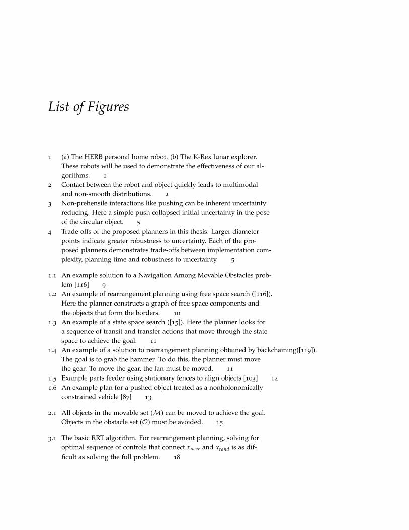
List of Figures
1 (a) The HERB personal home robot. (b) The K-Rex lunar explorer.These robots will be used to demonstrate the effectiveness of our al-gorithms. 1
2 Contact between the robot and object quickly leads to multimodaland non-smooth distributions. 2
3 Non-prehensile interactions like pushing can be inherent uncertaintyreducing. Here a simple push collapsed initial uncertainty in the poseof the circular object. 5
4 Trade-offs of the proposed planners in this thesis. Larger diameterpoints indicate greater robustness to uncertainty. Each of the pro-posed planners demonstrates trade-offs between implementation com-plexity, planning time and robustness to uncertainty. 5
1.1 An example solution to a Navigation Among Movable Obstacles prob-lem [116] 9
1.2 An example of rearrangement planning using free space search ([116]).Here the planner constructs a graph of free space components andthe objects that form the borders. 10
1.3 An example of a state space search ([15]). Here the planner looks fora sequence of transit and transfer actions that move through the statespace to achieve the goal. 11
1.4 An example of a solution to rearrangement planning obtained by backchaining([119]).The goal is to grab the hammer. To do this, the planner must movethe gear. To move the gear, the fan must be moved. 11
1.5 Example parts feeder using stationary fences to align objects [103] 12
1.6 An example plan for a pushed object treated as a nonholonomicallyconstrained vehicle [87] 13
2.1 All objects in the movable set (M) can be moved to achieve the goal.Objects in the obstacle set (O) must be avoided. 15
3.1 The basic RRT algorithm. For rearrangement planning, solving foroptimal sequence of controls that connect xnear and xrand is as dif-ficult as solving the full problem. 18
108 robust rearrangement planning using nonprehensile interaction
3.2 An example task. HERB must push the green box along the table intothe region denoted by the green circle. 21
3.4 In this scene the robot uses the whole arm to manipulate objects toachieve the goal. At several time points ((c), (d), (e)), the robot movesmultiple objects simultaneously. 23
3.3 Average distance to sample across 50 trials selecting random points. 23
3.7 In low clutter scenes, the planner still is able to use the whole armto manipulate the object. 24
3.5 The success rate of our algorithm compared with the Static RRT andDARRT. The graph depicts the expected success each algorithm achievesgiven any time budget up to 300 s. 24
3.6 The average planning time across all 350 trials for each planner. Failedtrials were assigned the max planning time (300s). As can be seen,the PCRRT reduces planning time. 24
3.8 In low clutter scenes, the DARRT planner can often solve the prob-lem trivially by applying a single primitive. 25
3.9 Success rate as a function of plan time for the scene from Fig.3.8. Inlow clutter scenes, primitive based planners such as DARRT outper-form our planner because a single primitive can trivially solve theproblem. 25
3.10 An example clearance task. HERB must move the 3 objects in the greenrectangle outside the rectangle in order to make space for placinga new item into the refrigerator. 25
3.11 In small cluttered space like the shelf of a refrigerator, empoweringthe planner to allow the robot to touch multiple objects simultane-ously and use the whole arm for interaction is critical to finding so-lutions. 26
3.12 The success rate of the PCRRT for the clearance tasks 26
3.13 Real robot experiments. Top Scene 1: The robot is able to achieve thegoal in all 10 executions of the trajectory. Bottom Scene 3. The robotfailed to achieve the goal in 3 of 10 attempts at executing the trajec-tory. These failures were due to small uncertainties in robot motionand initial object pose that led the robot to push the one of the bot-tles off of the edge of the table. 27
4.1 A breakdown of the time spent by the planner. 29
4.2 Parallelized tree search. 30
4.3 Average time for a single tree extension. As we increase the num-ber of controls considered at each extension (k) the improvementsfrom parallelization increase. 30
4.4 Average tree size after 10 s of tree growth. Increasing the availablethreads for simultaneous tree growth m increases the number of ex-tensions we can consider, growing the tree larger faster. 31
4.5 Average plan time across successful trials 31
rearrangement planning via heuristic search 109
4.6 Improvement in distance to a sampled configuration as we increasek, the number of sampled controls on each extension of the tree. Us-ing object-centric actions ( ) improves the extension quality over us-ing only robot-centric actions ( ). 32
4.7 An example failed “push-object” primitive. The desired end-effectorpose is not reachable. An alternate primitive that cages and pulls theobject must be defined for the planner to find a solution in object-centric
primitive based approaches. 33
4.8 Success rate as a function of plan time for HERB pushing objects ona table. 35
4.9 An example object-centric solution. The push primitive is used tomove the bowl in (b) and the box in (c)- (e). Other objects are movedthrough incidental contact during execution of push or transit prim-itives. 36
4.10 The K-Rex lunar explorer. 36
4.11 Two primitives defined for KRex. Dubins paths are used to gener-ate paths between two poses in SE(2). 37
4.12 The success rate as a function of plan time for each of the three KRextasks. The hybrid planner ( ) outperforms both the object-centric (and robot-centric ( ) planners across all tasks. 38
4.13 A robot-centric ( ) and object-centric ( ) solution easy scenes for eachtask. Left: The robot must traverse through an empty environmentto a goal region in the top right corner. Middle: The robot must pushthe blue box into a goal region in the top right corner. All green boxesare movable objects. Right The robot must push the green box fromits start pose in the middle of the environment to any pose outsidethe region outlined in green. 38
4.14 A single solution to a complex pushing task. Here the robot uses object-centric ( ) motions to make large advancements through the statespace. Robot-centric motions ( ) are used to back the robot away fromobstacles. 40
4.15 A single solution to a complex pushing task. Here the robot uses object-centric ( ) motions to make large advancements through the statespace. Robot-centric motions ( ) are used to back the robot away fromobstacles. 40
4.16 Execution of the object pushing task on the KRex rover 41
4.17 Execution of the clearance pushing task on the KRex rover 42
4.18 The success rate as a function of prand, the percentage of time robot-centric actions are used to grow the tree. 42
110 robust rearrangement planning using nonprehensile interaction
4.19 The shortcutting algorithm. For simplicity, we depict only the mo-tion of the end-effector. However, the whole arm is considered dur-ing planning. In (d) the motion of the manipulator and green objectremain unchanged along the remainder of the path. However, statesare updated to reflect the new location of the blue box and purplecircle. 43
4.20 Results from shortcutting for 15s. 43
4.21 An example shortcut. (b) The original path (dotted) contains unnec-essary extra movements removed in the shortcut path (solid). Thisleads to a new final pose of the robot and object (filled) when com-pared to the original (outline). (c) The shortcut also often leads toreduced motion of the object. 44
5.1 Examples for dynamic actions between statically stable states utilizedby humans. 48
5.2 Dynamic transitions between statically stable states in C 48
5.3 Three example scenes. In all three scenes, the robot must move thegreen object into the goal region denoted by a green circle. Blue ob-jects are movable. Red and orange objects are obstacles. 50
5.4 The success rate of the semi-dynamic planner with Tmax = 8 s andthe dynamic planner. Given a restricted time budget of 60 s, the semi-dynamic planner solves more scenes faster. 51
5.5 Success rate for different values of Tmax. 52
5.6 Average time to try a propagate a single extension of the tree. As Tmax
increases the propagation time increases. 52
5.7 Results for three scenes in Fig.5.3. (Left) Average path duration. (Note:Only one path was found for Tmax = 0 s in Scene 3) (Right) Successrate. 53
5.8 Top: Snapshots from a semi-dynamic trajectory lifted to a 7-DOF armtrajectory and executed on the robot in simulation (Tmax = 8s). Thetask is to move the green ball into the red goal. The orange boxes arestatic obstacles. The states marked with ∗ are statically stable. Mid-
dle: Velocity profile of the end-effector and the target. Note how therobot waits until the ball comes to rest before it performs the nextaction. Bottom: Velocities for a dynamic trajectory for the same scene.In contrast to the semi-dynamic trajectory the environment does notcome to rest after each action. 54
5.9 Top: Snapshots from a semi-dynamic trajectory lifted to a 7-DOF armtrajectory and executed on HERB (Tmax = 8s). The task is to movethe white box to the left. Bottom: Velocity profile for the trajectoryas planned. Multiple objects are pushed simultaneously. Also the tar-get object, the cup and one of the boxes are moved multiple times.The statically stable states are marked with ∗. 55
rearrangement planning via heuristic search 111
6.1 Three sources of uncertainty in the system. (a) and (b) are prevalentin many planning domains. Our framework introduces a third sourceof uncertainty: uncertainty in the physics model (c) 59
8.1 Rollouts of the control sequence can be used to estimate probabil-ity of success under uncertainty. 66
8.2 The successive rejects algorithm. During each phase, rollouts are per-formed on all remaining candidates to improve estimates of p for eachcandidate. After each phase, the candidate with lowest probabilityof success is eliminated. This continues until a single candidate re-mains in the set. 68
8.3 Histogram of the success probabilities achieved by 50 candidate con-trol sequences that solve the scene in Fig.8.4. 70
8.4 Start poses for the object in the scene are drawn from a Gaussian withdistribution µ = 0, Σ1/2 = diag{2cm, 2cm, 0.1rad}. The robot mustpush the box into the goal region. For simplicity, only the robot handis show, though contact is allowed with the full robot arm. 71
8.5 Achieved success probability as a function of budget for the scenein Fig.8.4. 71
8.6 The successive rejects algorithm finds better solutions than an algo-rithm that applies a fixed number of rollouts to every trajectory giventhe same budget B. 72
8.7 Comparison of the success probability estimated through Monte Carlorollouts (predicted) and observed during ten executions on the realrobot (actual). Trajectories with a high estimated probability of suc-cess tend to succeed more often when executed on the real robot. 72
8.8 Trajectory 7, from the results presented in Fig.8.7, executed on HERB.The trajectory selection algorithm chose to use a sweeping motionto robustly push the white box into the circular goal region. 73
8.9 Histogram of the success probabilities achieved by 50 candidate con-trol sequences that solve the scene in Fig.8.11. 73
8.10 The successive rejects algorithm finds better solutions than an algo-rithm that applies a fixed number of rollouts to every trajectory giventhe same budget B. 73
8.11 Success rate for two trajectories for the same clearance task. The toptrajectory is more robust to the control uncertainties prevalent forKRex. 74
9.1 An example pushing action that reduces uncertainty in object pose 75
9.2 Theor.9.1.1: Any trajectory within a radius r of a nominal ξ0 will con-verge to ξ0 if Dm < 0. 76
9.3 Test scenario. 80
112 robust rearrangement planning using nonprehensile interaction
9.4 Comparison of Ee values for the robot-centric (R), hybrid (H), B-RRTand CR-RRT. Increasing the bias in the C-RRT and decreasing the thresh-old in the CR-RRT both lead to better performing paths. 80
9.5 The success rate of the planners as a function of plan time. The in-creased computational burden of evaluating the divergence metricon each extension increases planning time and lowers success rateunder a fixed time budget. This highlights the trade-off required toproduce more robust paths. 80
9.6 Two example trajectories.Top: Exponential divergence Ee = 10.50.Bottom: Exponential divergence Ee = 0.15. 81
9.7 Measured success rate over 10 executions of trajectories on HERB asa function of exponential divergence, Ee. 81
9.8 Ee vs. pπ , the estimated probability of success used to guide trajec-tory selection in Ch.8, across all trajectories generated by the B-RRT.These two values are correlated: high Ee indicates low pπ . 82
10.2 The MCTS algorithm 85
10.1 The evolution of the uncertainty when performing a simple push-ing action. As can be seen, the uncertainty quickly becomes non-Gaussianand non-smooth. 85
10.3 A simple example of a hand pushing objects. The basic primitives al-low the hand to translate along the grid lines. In this simple exam-ple, the object is “trapped”, i.e. there are no primitives that allow itto move out of the cell. 88
10.4 An example of MCTS applied to rearrangement planning. A tree pol-
icy is used to select actions that make contact (top-right). Then thedefault policy plans in the a lower dimensional space (middle-right).The result is propagated through the full space to generate a reward(bottom-right). 89
10.6 An example path computed with the planned default policy (top)and random default policy (bottom) at t = 45 s. 92
10.5 Use of a policy explicitly seeking to achieve the goal ( ) results inoverall better paths when compared to using a policy that randomlyselects actions ( ) for both low clutter (top) and high clutter scenes(bottom). 92
10.7 An example path computed with the planned default policy (top)and random default policy (bottom) at t = 250 s. 93
10.8 Using contact primitives ( ) allows for finding better paths soonerthan using basic primitives ( ). 93
10.10In high clutter scenes, the UMCP algorithm with contact primitivesperforms well. The algorithm allows for increasing uncertainty inthe pose of the bowl, as long as it does not inhibit goal achievement. 94

rearrangement planning via heuristic search 113
10.9 On simple scenes (top), the B-RRT from Ch.9 ( ) is able to find bet-ter paths quickly. The UMCP algorithm ( ) is able to find better pathsmore quickly than the PCRRT from Ch.3 ( ). On difficult scenes (bot-
tom), the UMCP outperforms both the C-RRT and the PCRRT. 94

List of Tables
1.1 Planning among movable objects 12
2.1 Rearrangement planning terminology 15
3.1 Success counts for trajectories executed on the real robot. 26
4.1 Success rate and plan time for easy scenes. Plan times report meanand ± one standard deviation. 39
4.2 Average distance from goal center (cm) 41
4.3 Success rate of the clearance task. 42
9.1 Divergence metrics 77

B
Bibliography
[1] Open Dynamics Engine. http://www.ode.org, 2000 (accessedAugust 2014.
[2] NVIDIA PhysX: Physics simulation for developers. http:
//www.nvidia.com, 2009.
[3] Box2D. http://box2d.org, 2010 (accessed August 2014).
[4] Bullet physics library. http://bulletphysics.org, (accessedAugust 2014).
[5] P. Agarwal, J. Latombe, R. Motwani, and P. Raghavan. Non-holonomic path planning for pushing a disk among obstacles.In IEEE International Conference on Robotics and Automation, 1997.
[6] Y. Aiyama, M. Inaba, and H. Inoue. Pivoting: A new method ofgraspless manipulation of object by robot fingers. In IEEE/RSJ
International Conference on Intelligent Robots and Systems, 1993.
[7] S. Akella, W. H. Huang, K. M. Lynch, and M. T. Mason. Sen-sorless parts orienting with a one-joint manipulator. In IEEE
International Conference on Robotics and Automation, 1997.
[8] S. Akella and M. T. Mason. Posing polygonal objects in theplane by pushing. In IEEE International Conference on Robotics
and Automation, 1992.
[9] R. Alami, J. P. Laumond, and T. Siméon. Two manipulationplanning algorithms. In Workshop on the Algorithmic Foundations
of Robotics, 1994.
[10] R. Alterovitz, T. Siméon, and K. Goldberg. The stochasticmotion roadmap: A sampling framework for planning withmarkov motion uncertainty. In Robotics: Science and Systems,2007.
118 robust rearrangement planning using nonprehensile interaction
[11] J-Y Audibert and S. Bubeck. Best arm identification in multi-armed bandits. In COLT Conference on Learning Theory, 2010.
[12] P. Auer, N. Cesa-Bianchi, and P. Fischer. Finite-time analysis ofthe multiarmed bandit problem. Machine Learning, 47(2-3):235–256, 2002.
[13] H. Bai, D. Hsu, W. Lee, and A. Ngo. Monte carlo value it-eration for continuous-state POMDPs. In Workshop on the
Algorithmic Foundations of Robotics, 2010.
[14] J. Barraquand and J. Latombe. Nonholonomic multibodymobile robots: Controllability and motion planning in thepresence of obstacles. Algorithmica, 3:2328–2335, 1993.
[15] J. Barry, K. Hsiao, L. P. Kaelbling, and T. Lozano-Pérez. Manip-ulation with multiple action types. In International Symposium
on Experimental Robotics, 2012.
[16] J. Barry, L. P. Kaelbling, and T. Lozano-Pérez. A hierarchi-cal approach to manipulation with diverse actions. In IEEE
International Conference on Robotics and Automation, 2013.
[17] O. Ben-Shahar and E. Rivlin. Practical pushing planning forrearrangement tasks. In IEEE International Conference on Robotics
and Automation, 1998.
[18] O. Ben-Shahar and E. Rivlin. To push or not to push: On therearrangement of movable objects by a mobile robot. In IEEE
Transactions on Systems, Man and Cybernetics, 1998.
[19] D. Berenson, S.S. Srinivasa, D. Ferguson, A. Collet, and J.J.Kuffner. Manipulation planning with workspace goal regions.In IEEE International Conference on Robotics and Automation, 2009.
[20] D. Berenson, S.S. Srinivasa, D. Ferguson, and J. Kuffner. Manip-ulation planning on constraint manifolds. In IEEE International
Conference on Robotics and Automation, 2009.
[21] R-P Berretty, K. Goldberg, M.H. Overmars, and A. Frankvan der Stappen. Orienting parts by inside-out pulling. InIEEE International Conference on Robotics and Automation, 2001.
[22] B. Bonet and H. Geffner. Labeled RTDP: Improving the con-vergence of real-time dynamic programming. In International
Conference on Automated Planning and Scheduling, 2003.
[23] M. Brokowski, M. Peshkin, and K. Goldberg. Curved fences forpart alignment. In IEEE International Conference on Robotics and
Automation, 1993.

bibliography 119
[24] R. C. Brost. Automatic grasp planning in the presence of un-certainty. The International Journal of Robotics Research, 7(1):3–17,1988.
[25] C. Browne, E. Powley, D. Whitehouse, S. Lucas, P.I. Cowl-ing, P. Rohlfshagen, S. Tavener, D. Perez, S. Samothrakis, andS. Colton. A survey of Monte Carlo Tree Search methods. InIEEE Transactions on Computational Intelligence and AI in Games,2012.
[26] S. Caselli and M. Reggiani. ERPP: An experience-based ran-domized path planner. In IEEE International Conference on
Robotics and Automation, 2000.
[27] A.R. Cassandra. Exact and Approximate Algorithms for Partially
Observable Moarkov Decision Processes. PhD thesis, Departmentof Computer Science, Brown University, 1998.
[28] D. Challou, D. Boley, M. Gini, and V. Kumar. A parallel for-mulation of informed randomized search for robot motionplanning problems. In IEEE International Conference on Robotics
and Automation, 1995.
[29] L. Chang, S. Srinivasa, and N. Pollard. Planning pre-grasp ma-nipulation for transport tasks. In IEEE International Conference
on Robotics and Automation, 2010.
[30] G.M.J.-B. Chaslot, S. Bakkes, I. Szita, and P. Spronck. Monte-Carlo Tree Search: A new framework for game AI. In Artificial
Intelligence Interactive Digital Entertainment Conference, 2008.
[31] P. C. Chen and Y. K. Hwang. Practical path planning amongmovable obstacles. In IEEE International Conference on Robotics
and Automation, 1991.
[32] A. Cimatti and M. Roveri. Conformant planning via symbolicmodel checking. In Journal of Artificial Intelligence Research, 2000.
[33] M.R. Dogar, K. Hsiao, M. Ciocarlie, and S.S. Srinivasa. Physics-based grasp planning through clutter. In Robotics: Science and
Systems, 2012.
[34] M.R. Dogar and S.S. Srinivasa. Push-grasping with dexteroushands: Mechanics and a method. In IEEE/RSJ International
Conference on Intelligent Robots and Systems, 2010.
[35] M.R. Dogar and S.S. Srinivasa. A framework for push-graspingin clutter. In Robotics: Science and Systems, 2011.
120 robust rearrangement planning using nonprehensile interaction
[36] M.R. Dogar and S.S. Srinivasa. A planning framework fornon-prehensile manipulation under clutter and uncertainty.Autonomous Robots, 33(3):217–236, 2012.
[37] Arnaud Doucet, Nando de Freitas, and Neil Gordon. Sequential
Monte Carlo Methods in Practice. Springer Science & BusinessMedia, 2001.
[38] A. Dragan, N. Ratliff, and S.S. Srinivasa. Manipulation plan-ning with goal sets using constrained trajectory optimization.In IEEE International Conference on Robotics and Automation, 2011.
[39] L.E. Dubins. On curves of minimal length with a constrainton average curvature, and with prescribed initial and termi-nal positions and tangents. American Journal of Mathematics,79(3):497–516, 1957.
[40] M. Erdmann. An exploration of nonprehensile two-palmmanipulation: Planning and execution. Seventh International
Symposium on Robotics Research, 1995.
[41] M. A. Erdmann. Using backprojections for fine motion plan-ning with uncertainty. In IEEE International Conference on
Robotics and Automation, 1985.
[42] M.A. Erdmann and M.T. Mason. An exploration of sensorlessmanipulation. IEEE Journal of Robotics and Automation, 4(4):369–379, 1988.
[43] C. Van Geem, T. Siméon, and J-P. Laumond. Mobility analysisfor feasibility studies in cad models of industrial environments.In IEEE International Conference on Robotics and Automation, 1999.
[44] R.P. Goldman and M.S. Boddy. Expressive planning and ex-plicit knowledge. In International Conference on Artificial Intelli-
gence Planning and Scheduling, 1996.
[45] S. Goyal, A. Ruina, and J. Papadopoulos. Planar sliding withdry friction. Part 1. Limit surface and moment function. Wear,143:307–330, 1991.
[46] D.D. Grossman and M.W. Blasgen. Orienting mechanical partsby computer-controlled manipulator. In IEEE Transactions on
Systems, Man and Cybernetics, 1975.
[47] L.J. Guibas, D. Hsu, H. Kurniawati, and E. Rehman. Boundeduncertainty roadmaps for path planning. In Workshop on the
Algorithmic Foundations of Robotics, 2008.
bibliography 121
[48] M. Gupta and G.S. Sukhatme. Using manipulation primitivesfor brick sorting in clutter. In IEEE International Conference on
Robotics and Automation, 2012.
[49] P.E. Hart, N.J. Nillson, and B. Raphael. A formal basis forthe heuristic determination of minimum cost paths. In IEEE
Transactions on Systems Science and Cybernetics, 1968.
[50] P. Haslum and P. Jonsson. Some results on the complexity ofplanning with incomplete information. In European Conference
on Planning, 1999.
[51] K. Hauser and V. Ng-Thow-Hing. Fast smoothing of manipu-lator trajectories using optimal bounded-acceleration shortcuts.In IEEE International Conference on Robotics and Automation, 2010.
[52] J.A. Haustein, J.E. King, S.S. Srinivasa, and T. Asfour. Kino-dynamic randomized rearrangement planning via dynamictransitions between statically stable configurations. In IEEE
International Conference on Robotics and Automation, 2015.
[53] G. Havur, G. Ozbilgin, E. Erdem, and V. Patoglu. Geometric re-arrangement of multiple movable objects on cluttered surfaces:A hybrid reasoning approach. In IEEE International Conference
on Robotics and Automation, 2014.
[54] H. Hitakawa. Advanced parts orientation system has wideapplication. In Assembly Automation, 1988.
[55] R.D. Howe and M.R. Cutkosky. Practical force-motion modelsfor sliding manipulation. The International Journal of Robotics
Research, 15(6):557–572, 1996.
[56] W. Huang and M.T. Mason. Mechanics, planning, and con-trol for tapping. In Workshop on the Algorithmic Foundations of
Robotics, 1998.
[57] N. Hyafil and F. Bacchus. Conformant probabilistic planningvia CSPs. In International Conference on Automated Planning and
Scheduling, 2003.
[58] J. Ichnowski and R. Alterovitz. Parallel sampling-based motionplanning with superlinear speedup. In IEEE/RSJ International
Conference on Intelligent Robots and Systems, 2012.
[59] A. Johnson, J.E. King, and S.S. Srinivasa. Convergent planning.IEEE Robotics and Automation Letters, 1(2):1044–1051, 2016.
122 robust rearrangement planning using nonprehensile interaction
[60] Aaron M. Johnson, Samuel E. Burden, and D. E. Koditschek.A hybrid systems model for simple manipulation and self-manipulation systems. arXiv preprint arXiv:1502.01538 [cs.RO],2015.
[61] L. Kavraki and J-C Latombe. Randomized preprocessing ofconfiguration space for fast path planning. In IEEE International
Conference on Robotics and Automation, 1994.
[62] L. Kavraki, P. Svestka, J-C. Latombe, and M. Overmars. Prob-abilistic roadmaps for path planning in high dimensional con-figuration spaces. IEEE Transactions on Robotics and Automation,12(4):566–580, 1996.
[63] J.E. King, M. Cognetti, and S.S. Srinivasa. Rearrangementplanning using object-centric and robot-centric action spaces.In IEEE International Conference on Robotics and Automation, 2016.
[64] J.E. King, J.A. Haustein, S.S. Srinivasa, and T. Asfour. Non-prehensile whole arm rearrangement planning on physicsmanifolds. In IEEE International Conference on Robotics and Au-
tomation, 2015.
[65] J.E. King, M. Klingensmith, C. Dellin, M. Dogar, P. Velagapudi,N. Pollard, and S.S. Srinivasa. Pregrasp manipulation as trajec-tory optimization. In Robotics: Science and Systems, 2013.
[66] R.D. Kleinberg. Nearly tight bounds for the continuum-armedbandit problem. In Conference on Neural Information Processing
Systems, 2004.
[67] L. Kocsis and C. Szepesvári. Bandit based Monte-Carlo plan-ning. In European Conference on Machine Learning, 2006.
[68] M.C. Koval, M.R. Dogar, N.S. Pollard, and S.S. Srinivasa. Poseestimation for contact manipulation with manifold particlefilters. In IEEE/RSJ International Conference on Intelligent Robots
and Systems, 2013.
[69] M.C. Koval, J.E. King, N. Pollard, and S.S. Srinivasa. Robusttrajectory selection for rearrangement planning as a multi-armed bandit problem. In IEEE/RSJ International Conference on
Intelligent Robots and Systems, 2015.
[70] M.C. Koval, N.S. Pollard, and S.S. Srinivasa. Pre- and post-contact policy decomposition for planar contact manipulationunder uncertainty. In Robotics: Science and Systems, 2014.

bibliography 123
[71] A. Krontiris and K. Bekris. Dealing with difficult instances ofobject rearrangement. In Robotics: Science and Systems, 2015.
[72] A. Krontiris, R. Shome, A. Dobson, A. Kimmel, and K. Bekris.Rearranging similar objects with a manipulator using pebblegraphs. In IEEE-RAS International Conference on Humanoid
Robots, 2014.
[73] J.J. Kuffner and S.M. LaValle. RRT-Connect: An efficient ap-proach to single-query path planning. In IEEE International
Conference on Robotics and Automation, 2000.
[74] H. Kurniawati and V. Yadav. An online POMDP solver foruncertainty planning in dynamic environment. In International
Symposium on Robotics Research, 2013.
[75] N. Kushmerick, S. Hanks, and D.S. Weld. An algorithm forprobabilistic planning. 76:239–286, 1995.
[76] S.M. LaValle. Rapidly-exploring Random Trees: A new tool forpath planning. 1998.
[77] S.M. LaValle and J.J. Kuffner. Randomized kinodynamic plan-ning. The International Journal of Robotics Research, 20(5):378–400,2001.
[78] M. Levihn, J. Scholz, and M. Stilman. Planning with movableobstacles in continuous environments with uncertain dynam-ics. In IEEE International Conference on Robotics and Automation,2013.
[79] M. Likhachev and D. Ferguson. Planning long dynamically-feasible maneuvers for autonomous vehicles. In Robotics: Sci-
ence and Systems, 2008.
[80] Z. Littlefield, D. Klimenko, H. Kurniawati, and K. Bekris. Theimportance of a suitable distance function in belief-space plan-ning. In International Symposium on Robotics Research, 2015.
[81] Winfried Lohmiller and Jean-Jacques E Slotine. On contractionanalysis for non-linear systems. Automatica, 34(6):683–696, 1998.
[82] W. Lovejoy. A survey of algorithmic methods for partially ob-served Markov decision process. Annals of Operations Research,28(1):47–65, 1991.
[83] B. Luders, M. Kothari, and J.P. How. Chance constrained RRTfor probabilistic robustness to environmental uncertainty. InAIAA Guidance, Navigation, and Control Conference, 2010.
124 robust rearrangement planning using nonprehensile interaction
[84] K. Lynch. Locally controllable polygons by stable pushing. InIEEE International Conference on Robotics and Automation, 1997.
[85] K. Lynch. Toppling manipulation. In IEEE International Confer-
ence on Robotics and Automation, 1999.
[86] K. Lynch and M.T. Mason. Controllability of pushing. In IEEE
International Conference on Robotics and Automation, 1995.
[87] K. Lynch and M.T. Mason. Stable pushing: Mechanics, control-lability, and planning. In Workshop on the Algorithmic Founda-
tions of Robotics, 1995.
[88] K. Lynch and M.T. Mason. Dynamic nonprehensile manipu-lation: Controllability, planning and experiments. The Interna-
tional Journal of Robotics Research, 18(1):64–92, 1999.
[89] Y. Maeda, H. Kijimoto, Y. Aiyama, and T. Arai. Planning ofgraspless manipulation by multiple robot fingers. In IEEE
International Conference on Robotics and Automation, 2001.
[90] O. Maron and A.W. Moore. Hoeffding races: Acceleratingmodel selection search for classification and function approxi-mation. In Conference on Neural Information Processing Systems,1993.
[91] M.T. Mason. Mechanics and planning of manipulator pushingoperations. The International Journal of Robotics Research, 5(3):53–71, 1986.
[92] M.T. Mason. Progress in nonprehensile manipulation. The
International Journal of Robotics Research, 18(11):1129–1141, 1999.
[93] M.A. Melchior and R. Simmons. Particle RRT for path planningwith uncertainty. In IEEE International Conference on Robotics and
Automation, 2007.
[94] T. Mericli, M. Veloso, and H.L. Akin. Achievable push-manipulation for complex passive mobile objects using pastexperience. In International Conference on Autonomous Agents and
Multi-agent Systems, 2013.
[95] G. Monahan. A survey of partially observable markov decisionprocesses: Theory, models, and algorithms. Management Science,28(1):1–16, 1982.
[96] D. Nieuwenhuisen, A. Stappen., and M. Overmars. An effectiveframework for path planning amidst movable obstacles. InWorkshop on the Algorithmic Foundations of Robotics, 2008.
bibliography 125
[97] D. Nieuwenhuisen, A. Frank van der Stappen, and M.H. Over-mars. Path planning for pushing a disk using compliance.In IEEE/RSJ International Conference on Intelligent Robots and
Systems, 2005.
[98] Edwin Olson. AprilTag: A robust and flexible visual fiducialsystem. In IEEE International Conference on Robotics and Automa-
tion, pages 3400–3407, May 2011.
[99] J. Ota. Rearrangement planning of multiple movable objects byrealtime search methodology. In IEEE International Conference
on Robotics and Automation, 2002.
[100] J. Ota. Rearrangement planning of multiple movable objects -integration of global and local planning methodology. In IEEE
International Conference on Robotics and Automation, 2004.
[101] R. Pepy, M. Kieffer, and E. Walter. Reliable robust path planner.In IEEE/RSJ International Conference on Intelligent Robots and
Systems, 2008.
[102] M.A. Peshkin and A.C. Sanderson. The motion of a pushed,sliding workpiece. IEEE Journal of Robotics and Automation,4(6):569–598, 1988.
[103] M.A. Peshkin and A.C. Sanderson. Planning robotic manipula-tion strategies for workpieces that slide. IEEE Journal of Robotics
and Automation, 4(5):524–531, 1988.
[104] R. Platt, L.P. Kaelbling, T. Lozano-Pérez, and R. Tedrake. Effi-cient planning in non-Gaussian belief spaces and its applica-tion to robot grasping. In International Symposium on Robotics
Research, 2011.
[105] I. Pohl. Heuristic search viewed as path finding in a graph.Artificial Intelligence, 1970.
[106] S. Prentice and N. Roy. The belief roadmap, efficient planningin linear POMDPs by factoring the covariance. In International
Symposium on Robotics Research, volume 66, pages 293–305,2008.
[107] H. Robbins. Some aspects of the sequential design of experi-ments. Bulletin of the American Mathematical Society, 58(5):527–535, 1952.
[108] G. Sánchez and J-C. Latombe. On delaying collision checkingin PRM planning - application to multi-robot coordination. The
International Journal of Robotics Research, 21(1):5–26, 2002.
126 robust rearrangement planning using nonprehensile interaction
[109] K.M. Seiler, H. Kurniawati, and S.P.N Singh. An online andapproximate solver for POMDPs with continuous action space.In IEEE International Conference on Robotics and Automation, 2015.
[110] S. Sekhavat, P. Švestka, J.-P. Laumond, and M.H. Overmars.Multi-level path planning for nonholonomic robots using semi-holonomic subsystems. The International Journal of Robotics
Research, 17(8):840–857, 1998.
[111] D. Silver and J. Veness. Monte-carlo planning in largePOMDPs. In Conference on Neural Information Processing Sys-
tems, 2010.
[112] T. Siméon, J-P. Laumond, J. Cortés, and A. Sahbani. Manipu-lation planning with probabilistic roadmaps. The International
Journal of Robotics Research, 23(7–8):729–746, 2004.
[113] S.Jentzsch, A.Gaschler, O.Khatib, and A.Knoll. MOPL: Amulti-modal path planner for generic manipulation tasks.In IEEE/RSJ International Conference on Intelligent Robots and
Systems, 2015.
[114] D.E. Smith and D.S. Weld. Conformant graphplan. In AAAI
Conference on Artificial Intelligence, 1998.
[115] S.S. Srinivasa, D. Ferguson, C.J. Helfrich, D. Berenson, A. Col-let, R. Diankov, G. Gallagher, G. Hollinger, J. Kuffner, and M.V.Weghe. HERB: A Home Exploring Robotic Butler. Autonomous
Robots, 28(1):5–20, 2010.
[116] M. Stilman. and J. Kuffner. Navigation among movable ob-stacles: Real-time reasoning in complex environments. InIEEE-RAS International Conference on Humanoid Robots, 2004.
[117] M. Stilman and J. Kuffner. Planning among movable obsta-cles with artificial constraints. In Workshop on the Algorithmic
Foundations of Robotics, 2006.
[118] M. Stilman, K. Nishiwaki, S. Kagami, and J. Kuffner. Planningand executing navigation among movable obstacles. Springer
Journal of Advanced Robotics, 21(14):1617–1634, 2007.
[119] M. Stilman, J. Schamburek, J. Kuffner, and T. Asfour. Manipu-lation planning among movable obstacles. In IEEE International
Conference on Robotics and Automation, 2007.
[120] I. Sucan, M. Moll, and L. Kavraki. The Open Motion PlanningLibrary. IEEE Robotics and Automation Magazine, 19(4):72–82,2012.
bibliography 127
[121] S. Thrun. Monte Carlo POMDPs. In Conference on Neural
Information Processing Systems, 2000.
[122] J.N. Tsitsiklis. On the convergence of optimistic policy iteration.Journal of Machine Learning Research, 3:59–72, 2002.
[123] J. van den Berg, M. Stilman, J. Kuffner, M. Lin, andD. Manocha. Path planning among movable obstacles: a prob-abilistically complete approach. In Workshop on the Algorithmic
Foundations of Robotics, 2008.
[124] C.C. White. A survey of solution techniques for the partiallyobserved Markov decision process. Annals of Operations Re-
search, 32(1):215–230, 1991.
[125] G. Wilfong. Motion planning in the presence of movable obsta-cles. Annals of Mathematics and Artificial Intelligence, 41(4):764–790, 1991.
[126] S. Zickler and M. Velosa. Efficient physics-based planning:sampling search via non-deterministic tactics and skills. InInternational Conference on Autonomous Agents and Multi-agent
Systems, 2009.
[127] C. Zito, R. Stolkin, M. Kopicki, and J.L. Wyatt. Two-level RRTplanning for robotic push manipulation. In IEEE/RSJ Interna-
tional Conference on Intelligent Robots and Systems, 2012.
[128] N. Zumel and M. Erdmann. Nonprehensile two palm manip-ulation with non-equilibrium transitions between stable states.In IEEE International Conference on Robotics and Automation, 1996.
[129] N. Zumel and M. Erdmann. Nonprehensile manipulation fororienting parts in the plane. In IEEE International Conference on
Robotics and Automation, 1997.