SHAPE DETECTION BY PACKING CONTOURS Qihui Zhu

SHAPE DETECTION BY PACKING CONTOURS

Qihui Zhu

A DISSERTATION

in

Computer and Information Science

Presented to the Faculties of the University of Pennsylvania in Partial

Fulfillment of the Requirements for the Degree of Doctor of Philosophy

2010

Jianbo ShiSupervisor of Dissertation

Jianbo ShiGraduate Group Chairperson

Acknowledgements

First and foremost, I would like to thank my advisor, Prof. Jianbo Shi, for both his insight-

ful advice on research and sincere suggestions on my life andcareer. Through the years

at Penn, Jianbo has greatly broadened my scope on research. On the other hand, he has

offered numerous sharp comments that has kept me on the righttrack in science. Without

his persistent guidance and support, I would not have been gone this far in the adventure

of computer vision.

I am also grateful to all the members in my thesis committee: Camillo Jose Taylor,

Sanjeev Khanna, Jean Gallier at Penn, and Longin Jan Lateckifrom Temple University.

CJ organized the committee and gave extremely helpful advice on the overall presentation.

Sanjeev asked deep algorithmic questions that stimulate myfurther thinking on the topic.

Jean kindly provided with many suggestions on mathematics and writing (along with his

French humor). Longin inspired me in many aspects of contourbased shape detection,

which composes a major part of this thesis.

I have interacted with several wonderful faculty members inCIS department: Kostas

Daniilidis, Sampath Kannan, Ben Taskar, and Lawrence K. Saul. I would like to thank

Kostas for his warm encouragement and continuous support onmy research over these

years, Sampath and Ben for serving on my WPE-II committee andgiving me many valu-

able advices on primal-dual algorithms, and Lawrence for mentoring me on scientific

writing inside and outside his course.

Furthermore, my research work received much help from our talented and friendly

group members and alumni. I would like to thank Gang Song for all his spiritual and

technical support from day one, Praveen Srinivasan, LimingWang, and Yang Wu for their

ii

excellent collaboration on laying down the foundation of this work, Timothee Cour, Elena

Bernardis, Katerina Fragkiadaki, Jeffrey Byrne, Jack Sim,Weiyu Zhang, and Haifeng

Gong for their generous help on research and for making the lab a fun and nice place.

I am indebted to my other collaborators including PhilipposMordohai (Stevens), Stella

X. Yu (BC), Kilian Q. Weinberger (WUSTL), Fei Sha (USC), and Lawrence K. Saul

(again, now at UCSD). Philippos offered various help on the early draft of contour group-

ing (Chapter 2) and contour packing (Chapter 3), as well as other research projects. Stella

guided me on exploring many topics on perceptual organization and graph embedding.

The early work with Kilian, Fei and Lawrence on manifold embedding inspired me on the

computational solution of region packing (Chapter 6).

In addition, I was lucky enough to be surrounded and helped bycurrent and former

GRASP Lab members: Alexander Toshev, Mirko Visontai, Ameesh Makadia, Alexander

Patterson IV, Yuanqing Lin, Arvind Bhusnurmath, and Ben Sapp. I also cherish good

memories with my friends in CIS department including Tingting Sha, Qian Liu, Yi Feng,

Liming Zhao, Peng Li, Liang Huang, Stephen Tse, John Blitzer, Jinsong Tan, Mengmeng

Liu, Zhuowei Bao, Jianzhou Zhao, and many many others. I would like to give special

thanks to our graduate coordinator Michael Felker and administrative coordinator Charity

Payne for their assistance with all kinds of requests I brought up.

Last but also the most importantly, I would like to thank my family. My parents have

implanted in me the interest and passion on knowledge since childhood. I am grateful for

their endless love and continuous support in my career pursuit for so many years. This

thesis is dedicated to them.

iii

ABSTRACT

SHAPE DETECTION BY PACKING CONTOURS

Qihui Zhu

Jianbo Shi

Humans have an amazing ability to localize and recognize object shapes from nat-

ural images with various complexities, such as low contrast, overwhelming background

clutter, large shape deformation and signicant occlusion.We typically recognize object

shape as a whole the entire geometric conguration of image tokens and the context they

are in. Detecting shape as a global pattern involves two key issues: model representa-

tion and bottom-up grouping. A proper model captures long range geometric constraints

among image tokens. Contours or regions that are grouped from bottom-up capture cor-

relations of individual image tokens, and often appear as half complete shapes that are

easily recognizable. The main challenge of incorporating bottom-up grouping arises from

the representation gap between image and model. Fragmentedimage structures usually

do not correspond to semantically meaningful model parts.

This thesis presentsContour Packing, a novel framework that detects shapes in a global

and integral way, effectively bridging this representation gap. We rst develop a grouping

mechanism that organizes individual edges into long contours, by encoding Gestalt factors

of proximity, continuity, collinearity, and closure in a graph. The contours are character-

ized by their topologically ordered 1D structures, againstotherwise chaotic 2D image

clutter. Used as integral shape matching units, they are powerful for preventing accidental

alignment to isolated edges, dramatically reducing false shape detections in clutter.

We then propose a set-to-set shape matching paradigm that measures and compares

holistic shape congurations. Representing both the model and the image as a set of con-

tours, we seek packing a subset of image contours into a complete shape formed by model

contours. The holistic conguration is captured by shape features with a large spatial extent,

and the long-range contextual relationships among contours. The unique feature of this ap-

proach is the ability to overcome unpredictable contour fragmentations. Computationally,

iv

set-to-set matching is a hard combinatorial problem. We propose a linear programming

(LP) formulation for efciently searching over exponentially many contour congurations.

We also develop a primal-dual packing algorithm to quickly bound and prune solutions

without actually running the LPs.

Finally, we generalize set-to-set shape matching on more sophisticated structures aris

ing from both the model and the image. On the model side, we enrich the representation by

compactly encoding part conguration selection in a tree. This makes it applicable to holis-

tic matching of articulated objects with wild poses. On the image side, we extend contour

packing to regions, which has a fundamentally different topology. Bipartite graph packing

is designed to cope with this change. A formulation by semidenite program ming (SDP)

provides an efcient computational solution to this NP-hardproblem, and the exibility of

expressing various bottom-up grouping cues.

v

COPYRIGHT

Qihui Zhu

2010

Contents

Acknowledgements ii

1 Introduction 1

1.1 Motivation . . . . . . . . . . . . . . . . . . . . . . . . . . . . . . . . . . 2

1.2 Outline and Contributions . . . . . . . . . . . . . . . . . . . . . . . . .. 6

2 Contour Grouping 10

2.1 Overview . . . . . . . . . . . . . . . . . . . . . . . . . . . . . . . . . . 11

2.2 Untangling Cycle Formulation . . . . . . . . . . . . . . . . . . . . . .. 13

2.2.1 Directed Graph and Contour Grouping . . . . . . . . . . . . . . .13

2.2.2 Criteria for 1D Topological Grouping . . . . . . . . . . . . . .. 15

2.2.3 Circular Embedding . . . . . . . . . . . . . . . . . . . . . . . . . 19

2.3 Complex Eigenvectors: A Continuous Relaxation . . . . . . .. . . . . . 22

2.4 Random Walk Interpretation . . . . . . . . . . . . . . . . . . . . . . . .25

2.4.1 Periodicity . . . . . . . . . . . . . . . . . . . . . . . . . . . . . . 25

2.4.2 Persistent Cycles . . . . . . . . . . . . . . . . . . . . . . . . . . 26

2.5 Tracing Contours . . . . . . . . . . . . . . . . . . . . . . . . . . . . . . 28

2.5.1 Discretization . . . . . . . . . . . . . . . . . . . . . . . . . . . . 28

2.5.2 Untangling Cycle Algorithm . . . . . . . . . . . . . . . . . . . . 29

2.6 Experiments . . . . . . . . . . . . . . . . . . . . . . . . . . . . . . . . . 30

2.7 Summary . . . . . . . . . . . . . . . . . . . . . . . . . . . . . . . . . . 32

3 Contour Packing 36

3.1 Overview . . . . . . . . . . . . . . . . . . . . . . . . . . . . . . . . . . 37

vii

3.2 Set-to-Set Contour Matching . . . . . . . . . . . . . . . . . . . . . . .. 39

3.2.1 Problem Formulation . . . . . . . . . . . . . . . . . . . . . . . . 39

3.2.2 Context Selective Shape Features . . . . . . . . . . . . . . . . .. 42

3.2.3 Contour Packing Cost . . . . . . . . . . . . . . . . . . . . . . . . 44

3.3 Computational Solution via Linear Programming . . . . . . .. . . . . . 46

3.3.1 Single Point Figure/Ground Selection . . . . . . . . . . . . .. . 46

3.3.2 Joint Contour Selection . . . . . . . . . . . . . . . . . . . . . . . 48

3.4 Related Work and Discussion . . . . . . . . . . . . . . . . . . . . . . . .51

3.5 Experiments . . . . . . . . . . . . . . . . . . . . . . . . . . . . . . . . . 53

3.6 Summary . . . . . . . . . . . . . . . . . . . . . . . . . . . . . . . . . . 55

4 The Primal-Dual Packing Algorithm 57

4.1 Primal-Dual Combinatorial Algorithms . . . . . . . . . . . . . .. . . . . 58

4.2 Primal-Dual Algorithms for Packing and Covering . . . . . .. . . . . . . 59

4.2.1 Multiplicative Weight Update: From Primal to Dual . . .. . . . . 61

4.2.2 The Oracle: From Dual to Primal . . . . . . . . . . . . . . . . . . 63

4.2.3 Complexity Analysis . . . . . . . . . . . . . . . . . . . . . . . . 64

4.3 Primal-Dual Formulation for Contour Packing . . . . . . . . .. . . . . . 65

4.4 Implementation . . . . . . . . . . . . . . . . . . . . . . . . . . . . . . . 68

4.5 Summary . . . . . . . . . . . . . . . . . . . . . . . . . . . . . . . . . . 71

5 Contour Packing with Model Selection 72

5.1 Overview . . . . . . . . . . . . . . . . . . . . . . . . . . . . . . . . . . 73

5.2 Related Work . . . . . . . . . . . . . . . . . . . . . . . . . . . . . . . . 75

5.3 Holistic Shape Matching . . . . . . . . . . . . . . . . . . . . . . . . . . 76

5.3.1 Formulation of Pose Estimation Problem . . . . . . . . . . . .. . 76

5.3.2 Generation of Model Active Descriptors . . . . . . . . . . . .. . 78

5.4 Computational Solution for Matching Holistic Features. . . . . . . . . . 80

5.5 Experiments . . . . . . . . . . . . . . . . . . . . . . . . . . . . . . . . . 82

5.6 Summary and Future Work . . . . . . . . . . . . . . . . . . . . . . . . . 83

viii

6 Region Packing 86

6.1 Overview . . . . . . . . . . . . . . . . . . . . . . . . . . . . . . . . . . 87

6.2 Holistic Region Matching . . . . . . . . . . . . . . . . . . . . . . . . . .89

6.2.1 Bipartite Graph Packing . . . . . . . . . . . . . . . . . . . . . . 90

6.2.2 Approximation via Semidefinite Program (SDP) . . . . . . .. . . 92

6.3 Representing Grouping Constraints . . . . . . . . . . . . . . . . .. . . . 94

6.3.1 Figure/Ground . . . . . . . . . . . . . . . . . . . . . . . . . . . 95

6.3.2 Boundary Saliency . . . . . . . . . . . . . . . . . . . . . . . . . 95

6.3.3 Junction Configurations . . . . . . . . . . . . . . . . . . . . . . . 98

6.4 Experiments . . . . . . . . . . . . . . . . . . . . . . . . . . . . . . . . . 99

6.4.1 Implementation . . . . . . . . . . . . . . . . . . . . . . . . . . . 100

6.4.2 Quantitative Comparison . . . . . . . . . . . . . . . . . . . . . . 101

6.5 Summary . . . . . . . . . . . . . . . . . . . . . . . . . . . . . . . . . . 104

7 Conclusion 111

A Appendix 114

A.1 Proof of Theorem 2.1 . . . . . . . . . . . . . . . . . . . . . . . . . . . . 114




A.5 Proof of Corollary 4.2 . . . . . . . . . . . . . . . . . . . . . . . . . . . . 122



References 126

ix

List of Tables

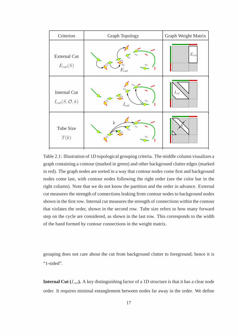
2.1 Illustration of 1D topological grouping criteria. The middle column vi-

sualizes a graph containing a contour (marked in green) and other back-

ground clutter edges (marked in red). The graph nodes are sorted in a way

that contour nodes come first and background nodes come last,with con-

tour nodes following the right order (see the color bar in theright column).

Note that we do not know the partition and the order in advance. Exter-

nal cut measures the strength of connections leaking from contour nodes

to background nodes shown in the first row. Internal cut measures the

strength of connections within the contour that violates the order, shown

in the second row. Tube size refers to how many forward step onthe cycle

are considered, as shown in the last row. This corresponds tothe width of

the band formed by contour connections in the weight matrix.. . . . . . 17

3.1 Comparison of Precision/Recall (P/R). We compare the precision of our

approach to the precision in (Ferrariet al.., 2007) at the same recall (lower

recall in (Ferrariet al.., 2007)). We convert the result of (Ferrariet al..,

2007) reported in DR/FPPI into P/R since the number of imagesin each

class is known. Our performance is significantly better than(Ferrariet al..,

2007) in four out of five classes. The other class ”Mugs” have some in-

stances that are too small to be detected by contour grouping. Note that

we did not use magnitude information which plays an important role in

(Ferrariet al.., 2007). . . . . . . . . . . . . . . . . . . . . . . . . . . . . 52

x

6.1 Comparison of region packing and the latest shape detection works on av-

erage precision (AP).†: Same train/test split as (Srinivasanet al. 2010),

i.e. taking 50% positives as training examples, with the same number of

negatives randomly sampled from other categories.§: Same region pack-

ing algorithm as†, but split train/test as (Toshevet al. 2010), which in-

cludes 50% images as training set (larger than (Srinivasanet al.2010)). . 102

6.2 The effect of different factors in region packing. . . . . .. . . . . . . . 104

xi

List of Figures

1.1 Complexities in real images. In (a), part of the mug is covered by shadow.

The contour of the starfish in (b) is surrounded by both clutter in the back-

ground, and texture in the foreground. The baseball player in (c) has a

very different pose than the canonical model. Part of the bottle in (d) is

occluded by a person’s hand. Despite all these complexities, a human has

no difficulty in locating and matching objects to the target shape models

shown at the top left corner. . . . . . . . . . . . . . . . . . . . . . . . . . 1

1.2 The global percept of shapes. (a) presents a simple shapewith a silhouette.

Image tokens that fits to the target locally could compose a completely

different shape as shown in (b). The local neighborhoods of (a) and (b)

marked in green have identical junctions, with the curvature of the smooth

silhouettes similar in most of the places. Matching shapes by aligning

edges independently could contrive false hypotheses as shown in (c). Most

of the silhouette in (a) can be aligned to some individual edges in (c). They

group with the horizontal lines as integral contours, and those lines do not

have matches to the target. In (d), although part of the object silhouette is

also missing, most likely the object has the same shape as thetarget, and

missing silhouette is only due to occlusion. . . . . . . . . . . . . .. . . 2

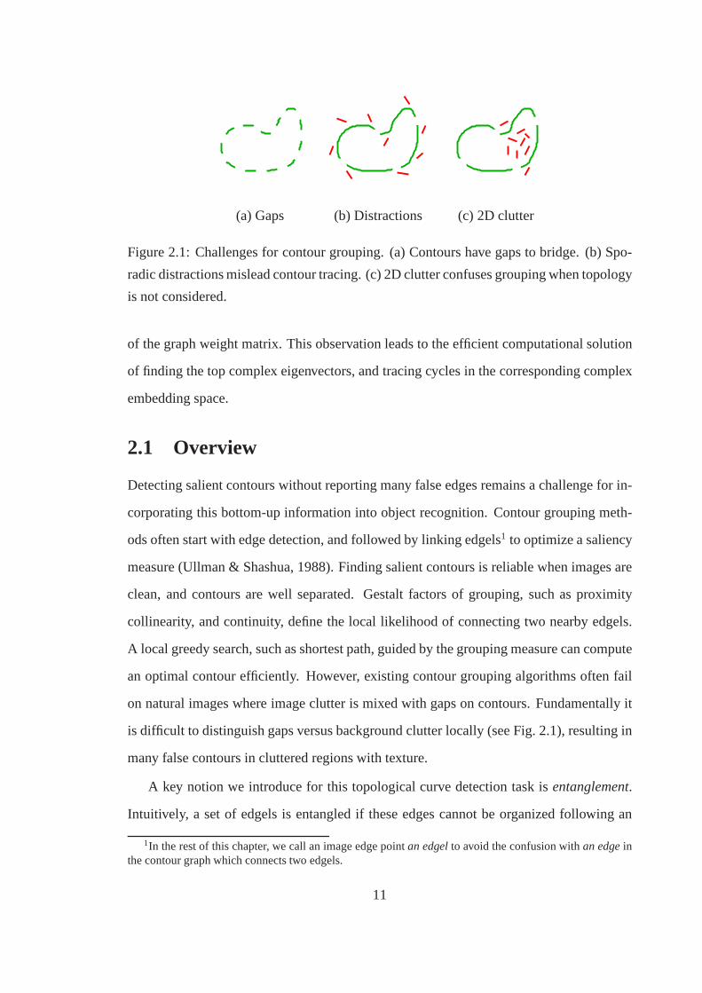
2.1 Challenges for contour grouping. (a) Contours have gapsto bridge. (b)

Sporadic distractions mislead contour tracing. (c) 2D clutter confuses

grouping when topology is not considered. . . . . . . . . . . . . . . .. . 11

xii

2.2 Distinction of 1D vs 2D topology. (a) The 2D topology (e.g. regions)

assumes a clique model. In (b), (c) The 1D topology assumes a chain or a

cycle model. A ring has a 1D topology but is geometrically embedded in

2D. . . . . . . . . . . . . . . . . . . . . . . . . . . . . . . . . . . . . . . 13

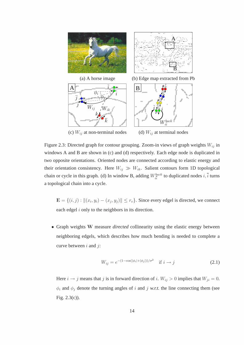
2.3 Directed graph for contour grouping. Zoom-in views of graph weights

Wij in windows A and B are shown in (c) and (d) respectively. Each

edge node is duplicated in two opposite orientations. Oriented nodes are

connected according to elastic energy and their orientation consistency.

HereWij ≫ Wik. Salient contours form 1D topological chain or cycle in

this graph. (d) In window B, addingW backii

to duplicated nodesi, i turns a

topological chain into a cycle. . . . . . . . . . . . . . . . . . . . . . . . 14

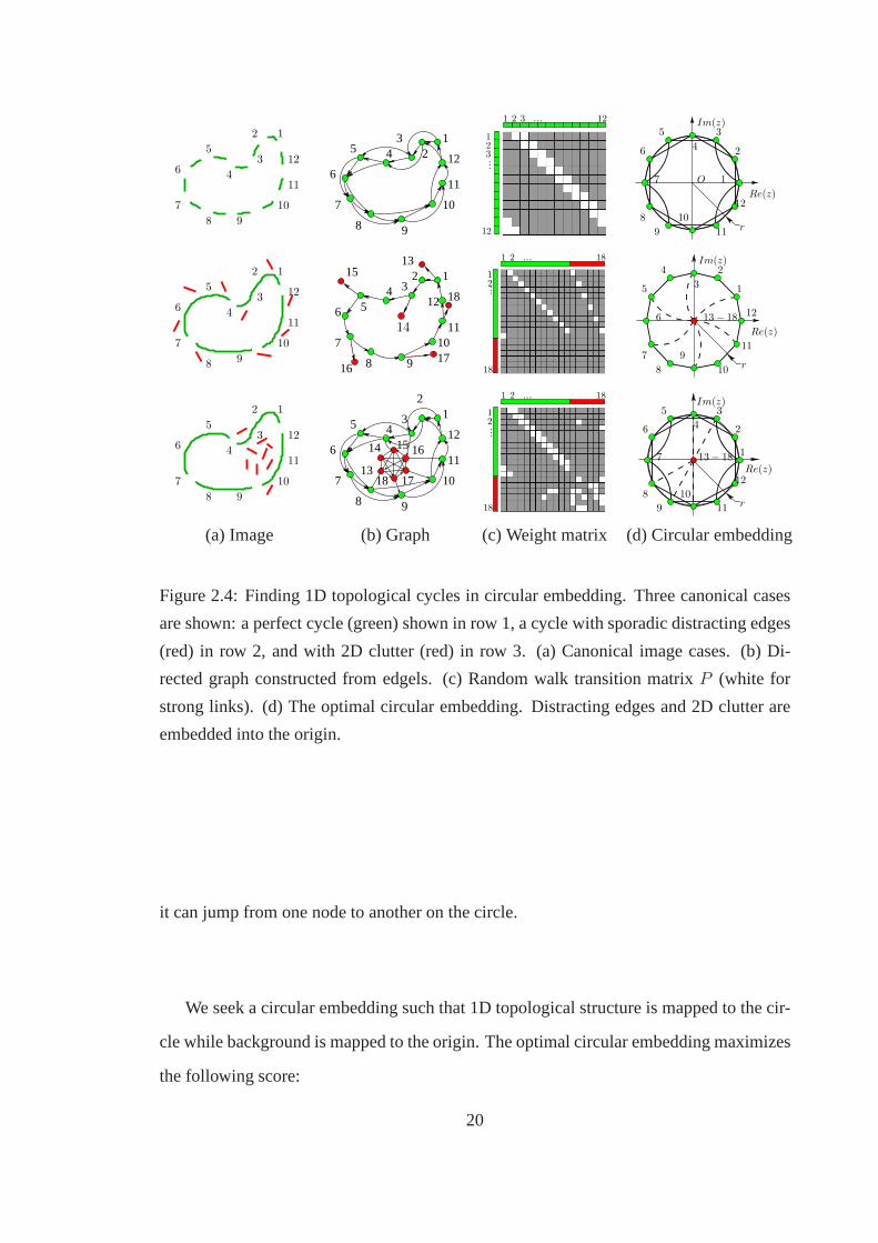
2.4 Finding 1D topological cycles in circular embedding. Three canonical

cases are shown: a perfect cycle (green) shown in row 1, a cycle with spo-

radic distracting edges (red) in row 2, and with 2D clutter (red) in row 3.

(a) Canonical image cases. (b) Directed graph constructed from edgels.

(c) Random walk transition matrixP (white for strong links). (d) The op-

timal circular embedding. Distracting edges and 2D clutterare embedded

into the origin. . . . . . . . . . . . . . . . . . . . . . . . . . . . . . . . 20

2.5 Persistent cycles. (a) 1D contours correspond to good cycles. (b) Re-

turning probabilityPr(i, t) on 1D contours has period peaks since random

walk on it tends to return in a fixed time. (c) 2D clutter corresponds to bad

cycles. (d) Returning probabilityPr(i, t) of random walk on 2D clutter is

flat. . . . . . . . . . . . . . . . . . . . . . . . . . . . . . . . . . . . . . . 24

2.6 Peakness measure.R(i, T ) measures the ’peakness’ of the returning prob-

ability Pr(i, T ) of random walk in the graph. It can be shown thatR(i, T )

is dominated by complex eigenvalues of the random walk matrix P . . . . 26

xiii

2.7 Illustration of computational solution.(a) An elephant with a detected con-

tour grouping (green) and endpoints (yellow) on its tusk. (b) The topnc

eigenvalues sorted by their real components. Their phase angles relate to

the 1D thickness of cycles. We look for complex ones with large magni-

tudes but small phase angles indicating the existence of thin 1D structures.

(c) The complex eigenvector corresponding to the selected eigenvalue in

(b) (red circle) is plotted. The detected tusk contour is embedded into a

geometric cycle plotted in red. We find discretization in this embedding

space by seeking the maximum circular cover shown in (d). . . .. . . . . 27

2.8 Precision recall curve on the Berkeley benchmark, with comparison to

Pb, CRF and min cover. We use probability boundary with low threshold

to produce graph nodes, and seek untangling 1D topological cycles for

contour grouping. The same set of parameters are used to generate all the

results. . . . . . . . . . . . . . . . . . . . . . . . . . . . . . . . . . . . 30

2.9 Contour grouping results on real images. Our method prunes clutter edges

(dark), and groups salient contours (bright). We focus on graph topology,

and detect contours that are either open or closed, straightor bended. . . 33

2.10 Contour grouping results on Weizmann horse database. All detected bi-

nary edges are shown (right). Our method prune clutter edges(dark), and

groups salient contours (bright). We use no edge magnitude information

for grouping, and can detect faint but salient contours under significant

clutter. We focus on graph topology, and detect contours that are both

open or closed, straight or bent. . . . . . . . . . . . . . . . . . . . . . . 34

2.11 Contour grouping results on Berkeley baseball player dataset. . . . . . . 35

xiv

3.1 Typical false positives can be traced to two causes: (1) Accidental align-

ment shown in (a). Our algorithm prunes it by exploiting contour integrity,

i.e. requiring contours to be whole-in/whole-out. Contours violating this

constraint is marked in white on the image. (2) Missing critical object

parts indicates that the matching is a false positive. In (b), after removing

the accidental alignment to the apple logo outline (marked in white), only

the body can find possible matches and the neck of the swan is completely

missing shown at the top-right corner of (b). Our approach rejects this

type of detection by checking missing critical model contours after joint

contour selection. . . . . . . . . . . . . . . . . . . . . . . . . . . . . . . 37

3.2 Using a single line drawing object model shown in (c), we detect object in-

stances in images with background clutter in (a) using shape. Bottom-up

contour grouping provides tokens of shape matching. Long salient con-

tours in (b) can generate distinctive shape descriptions, allowing both ef-

ficient and accurate matching. Image and model contours, shown by dif-

ferent colors in (b) and (c), do not have one-to-one correspondences. We

formulate shape detection as a set-to-set matching task in (d) consisting of:

(1) correspondences between control points, and (2) selection of contours

that contribute contextual shape features to those controlpoints, within a

disk neighborhood. . . . . . . . . . . . . . . . . . . . . . . . . . . . . . 40

xv

3.3 Illustration of our computational solution for set-to-set contour matching

on shape detection example from Fig. 3.2. The top and the bottom row

shows the image and model contour candidate sets marked in gray. Each

contour contributes its shape information to nearbycontrol pointsin the

form of Shape Context histogram, shown on the right. By selecting dif-

ferent contours (xsel, ysel), each control point can take on a set of possible

Shape Context descriptions (scI , scM ). With the correct contour selection

in the image and model (marked by colors), there is a one-to-one cor-

respondenceU corij between (a subset of) image and model control points

(marked by symbols). This is a computationally difficult search problem.

The efficient algorithm we developed is based on an encoding of Shape

Context description (which could take on exponentially many possible val-

ues) using linear algebraic formulation on the contour selection indicator:

scI = V I · xsel. This leads to the LP optimization solution. . . . . . . . . 43

3.4 Illustration of contour packing for shape detection. From input image (a),

we detect long salient contours shown in (b). For each control point cor-

respondence in (c), we select foreground contours whose global shape is

most similar to the model, with selectionxsel shown in gray scale (the

brighter, the largerxsel). Voting maps in (c) prune geometrically inconsis-

tent correspondences. (d) shows the consistent correspondences marked

by different colors. The optimal joint contour selection isshown in (e).

Note in the last example, model selection allows us to detectfalse match

on the face. . . . . . . . . . . . . . . . . . . . . . . . . . . . . . . . . . 45

xvi

3.5 Precision vs. recall curves on five classes of ETHZ Shape Classes. Our

precisions on ”Applelogos”, ”Bottles”, ”Giraffes” and ”Swans” are con-

siderably better than results in (Ferrariet al.., 2007): 49.3%/32.6% (Ap-

plelogos), 65.4%/33.3% (Bottles), 69.3%/43.9% (Giraffes) and 31.3%/23.3%

(Swans). Also notice that we boost the performance by large amount com-

pared to local shape context voting without contour selection. . . . . . . . 54

3.6 Examples of contour context selection on model and imagecontours in

ETHZ Shape Classes. The first five rows show detected objects from im-

age with significant background clutter. In the last row, thefirst four cases

are false positives successfully pruned by our algorithm bychecking the

configurations of selected model contours. The last two are failure cases.

Each image only displays one detected object instance. . . . .. . . . . . 56

4.1 Performance of primal-dual packing algorithm. Single point figure/ground

selection is run in6 scales to detect the swan shape in (a). The number

of model control points ranges from5 to 35. (b) shows the number of

hypotheses to search in all the scales when the number of model control

points is28, with scale4 marked in diamond (the scale in which the swan is

detected). (c) shows the proportion of correspondences handled by primal-

dual iterations (line 3) and interior point iterations (line 7) in Algorithm 4.

In (d), the running time of the entire algorithm is shown and compared to

the one without primal-dual pruning. Note that the rejection by primal-

dual iterations consumes very little time in the algorithm.. . . . . . . . . 70

5.1 Given an image (a), salient contours are extracted (b) from the edge map of

Pb Having contours as our unit, we use a coupled optimizationprocedure

of foreground contour selection and model deformation to recover the pose

of an articulated baseball player (c). . . . . . . . . . . . . . . . . . .. . 74

xvii

5.2 Holistic shape matching. Our search has two parallel process, each en-

coded by a selection variable. On the image side (left), contour selection

variables turn image contours ON and OFF assigning them to foreground

or background respectively. This results in all feasible shapes on the im-

age side. On the model side, selection variables assign configurations to

each model part in the tree structure. The two shapes, one derived from the

image and one from the model, are compared to each other usinga holistic

shape feature. When the two match, recognition and pose estimation are

achieved. Therefore the recognition task amounts to findingthe optimal

selection on both the image and the model side. . . . . . . . . . . . .. . 76

5.3 Object model and articulation. The model deformationΘ is controlled by

joint positions. Once positions of two adjacent jointsa andb are deter-

mined, shown ini andj in (b), the part can deform accordingly. This type

of deformation can be encoded by the selection variableyabij on the model

side. Continuous relaxation using LP produces sketch-likerough pose es-

timations of parts, marked by different colors in (c). Note that for most

parts, the values ofyabij are very small. (b) also shows the sum ofyab

ij at all

the sample locations for one joint, with red for large valuesand blue for

small values. These values give the confidence of the joint locations. In

this case, it correctly locates the knee. . . . . . . . . . . . . . . . .. . . 78

5.4 Comparison on baseball dataset. Joints with medial axesare displayed

on top of the image. Subplots from left to right are: (a) Original image;

(b) Results of our approach using large shape context windowbut without

context selection; (c) Results of our approach using a smallwindow again

without context selection; (d) Results in (Ramanan, 2007);(e) Results of

our approach. Our approach is able to discover the correct rough poses in

spite of large pose variations. . . . . . . . . . . . . . . . . . . . . . . . .84

xviii

5.5 More results on baseball dataset. Joints with medial axes are displayed

on top of the image. Subplots from left to right are: (a) Original image;

(b) Results of our approach using large shape context windowbut without

context selection; (c) Results of our approach using a smallwindow again

without context selection; (d) Results in (Ramanan, 2007);(e) Results of

our approach. Our approach is able to discover the correct rough poses in

spite of large pose variations. . . . . . . . . . . . . . . . . . . . . . . . .85

6.1 Overview of region packing. The first row shows the input image and

model with different boundary fragmentations. In the second row, we con-

struct bipartite subgraphs whose nodes are foreground and background

regions respectively. The figure/ground partitioning generates bipartite

subgraphs, whose edges correspond to boundary fragments (marked with

color in the graph). Our goal is to pack these bipartite edgessuch that the

overall shapes from image and model are a good match. . . . . . . .. . 90

6.2 Figure/ground labeling on boundaries. The boundary of aswan along with

its foreground region is shown in (a). In the circled area, different fig-

ure/ground configurations exist and need to be distinguished. Two true

boundaries with opposite directions in (b) and (c) appear due to the paral-

lelism. (d) shows a false boundary with incorrect figure/ground labeling. . 94

6.3 Binary region boundaries alone are insufficient to pop upobject shapes.

(a) shows an image containing mugs and bowls clearly discernible from

background. Restricted to binary region boundaries in (b),objects are sur-

rounded by fake boundaries in the background (lower part of the image),

and hence become less salient. In (c), boundary saliency helps to re-group

over-fragmentations of objects. Segmentation boundariesare colored by

strengths from low (blue) to high (red). . . . . . . . . . . . . . . . . .. 96

xix

6.4 Illustration of the junction configuration and a false positive. (a) shows

an accidental alignment of the swan, where the region boundaries make a

wrong turn without paying large penalties (marked in yellowrectangles).

The boundary strengths computed by eq. (6.20) are also displayed on the

figure, increasing from blue to red. A schematic diagram of regions is

shown in (b). Region packing only chooses regionrj (+1/ − 1 means

foreground/background). This creates an incorrect boundary fragment and

makes the strong boundary leak to the background. Note that astrong

boundary leaking to the foreground is very likely due to a salient object

part (top part of the mug in (c), (d)), and a weak object boundary. . . . . 98

6.5 Precision vs. Recall curves (PR). . . . . . . . . . . . . . . . . . . .. . . 104

6.6 Top 20 detections on Applelogos. Detections are sorted by scores from

high to low. The continuous values of region selection indicator are col-

ored on the corresponding regions from white (−1) to red (1). . . . . . . . 105

6.7 Top 20 detections for Bottles. Detections are sorted by scores from high

to low. The continuous values of region selection indicatorare colored on

the corresponding regions from white (−1) to red (1). . . . . . . . . . . . 106

6.8 Top 20 detections for Giraffes. Detections are sorted byscores from high



6.9 Top 20 detections for Mugs. Detections are sorted by scores from high to

low. The continuous values of region selection indicator are colored on


6.10 Top 20 detections for Swans. Detections are sorted by scores from high



6.11 Typical misses for all five categories. True positives with the lowest scores.

The figures are sorted by score in ascending order from top to bottom. . . 110

xx

A.1 Reduction from packing to MaxCut. (a) is a simple case where there is

only one bin. The red blocks represent image contours nodesI. The green

blocks are nodes for model partsM and the yellow nodes is the fictitious

node{V0}. Image or model background nodes are shaded. (b) shows the

corresponding graph cut of the packing. . . . . . . . . . . . . . . . . .. 117

xxi

Chapter 1

Introduction

Humans have an amazing ability to localize and recognize object shapes from an image

with various complexities, such as low contrast, overwhelming background clutter, large

shape deformation, and significant occlusion (see Fig. 1.1). Shape is not only a useful cue

for object recognition, but also an important problem by itself because it leads to further

understanding of the geometric arrangement of the scene, and functional properties of

objects.

(a) Low contrast (b) Background clutter (c) Deformation (d)Occlusion

Figure 1.1: Complexities in real images. In (a), part of the mug is covered by shadow.

The contour of the starfish in (b) is surrounded by both clutter in the background, and

texture in the foreground. The baseball player in (c) has a very different pose than the

canonical model. Part of the bottle in (d) is occluded by a person’s hand. Despite all these

complexities, a human has no difficulty in locating and matching objects to the target

shape models shown at the top left corner.

1

(a) Model (b) Matching locally (c) Matching in isolation (d)Occlusion

Figure 1.2: The global percept of shapes. (a) presents a simple shape with a silhouette.

Image tokens that fits to the target locally could compose a completely different shape as

shown in (b). The local neighborhoods of (a) and (b) marked ingreen have identical junc-

tions, with the curvature of the smooth silhouettes similarin most of the places. Matching

shapes by aligning edges independently could contrive false hypotheses as shown in (c).

Most of the silhouette in (a) can be aligned to some individual edges in (c). They group

with the horizontal lines as integral contours, and those lines do not have matches to the

target. In (d), although part of the object silhouette is also missing, most likely the object

has the same shape as the target, and missing silhouette is only due to occlusion.

1.1 Motivation

Shape is fundamentally aglobal percept– we typically recognize object shape as a whole.

By “global” we mean the following two concepts:

1. Non-locality. Shapes are measured by theentiregeometric configuration of image

tokens, rather than their local properties. Unlike other object properties such as

texture, a shape hardly has small distinctive parts that canuniquely identify it.

2. Non-isolation.Shapes are formed by orderly structures thatlink image tokens to-

gether, instead of independent image tokens. Grouping on these tokens provides a

context where the shape could be extended, and what could be the other alternatives.

Fig. 1.2 illustrates false shape matching examples ignoring either one of these two aspects.

An image hypothesis can locally fit the shape prototype in most of the places, but overall

does not resemble the target at all. On the other hand, a subset of individual edges can be

aligned to the prototype perfectly, but edges connected to them do not have matches, and

2

cause errors faraway from the matched edges.

In light of the above observations,model representationandbottom-up groupingare

key issues to consider in order to detect shapes robustly from images. A proper model

representation handles the non-locality problem by capturing long range geometric con-

straints. During the search process, image tokens that are far apart can be bound by the

model, interpreted and checked via their configurations. Bottom-up image structures such

as contours identify the underlying correlation of individual edges, which can be extracted

from the image independent of the shape model. Matching withthese integral shape to-

kens avoids many accidental alignments to isolated edges inthe clutter.

Previous shape detection and matching approaches can be classified into two groups

by model representation: shape primitive based methods andtemplate-based methods.

Shape primitive based methods.These approaches assume that shapes are composed

of some high level generic primitives, or volumetric parts that constitute objects via cer-

tain basic rules. These components include generalized cylinders (Brooks, 1983), su-

perquadratics (Pentland, 1986), geons (Biederman, 1985),and ribbons (Nevatia & Bin-

ford, 1977). Although perceptually these primitives make proper abstraction of the shape

models, they are hard to detect from images reliably. The representation gap between the

model and the image poses a big challenge: a shape recognition system has to connect

raw image edges or pixels into contours or surfaces, and thenassemble them into these

high level primitives. This results in two typical problemswhich eclipses the application

of these methods in real images. First, previous search procedures such as Interpretation

Tree (Grimson & Lozano-Perez, 1987) are insufficient to explore the huge, usually expo-

nential, solution space. Second, many premature hard decisions have to be made before

reaching the final output since the primitives are several levels above the image pixels.

Medial axis based representations (Blum, 1967; Peleg & Rosenfeld, 1981; Leymarie &

Levine, 1992; Baiet al., 2007) continue on the path of these attempts to develop highlevel

primitives. Several shape descriptions such as Shock Graphs (Siddiqiet al. , 1999) and

Poisson equation based features (Gorelicket al. , 2006) effectively capture global shapes

3

as well as semantical parts. Because medial axes are sensitive to region boundaries, all

these approaches assume that object regions and their boundaries have been segmented

from the background. However, segmenting foreground objects correctly is a hard prob-

lem to solve on its own in shape detection. Medial axis is a useful representation for

describing and matching holistic shapes given the foreground regions, but does not pro-

vide insights on how to search the target shape from image regions with over-segmentation

or under-segmentation.

Template-based methods.A separate path of research has been focusing on building

shape templates by low level, and detectable tokens. This essentially brings the model

representation all the way down to the image, such that the patterns of model representa-

tion are repeatable in images. For example, the tokens can beas simple as edge points.

Chamfer matching (Barrowet al. , 1977; Shottonet al. , 2008) and Hausdorff matching

(Huttenlocheret al. , 1993) are representatives of when the model is merely a set of un-

ordered points with fixed locations. The tokens can also be keypoints along with local

shape or appearance descriptors. Shapes are represented asthe spatial configurations of

these keypoints,e.g.geometric hashing (Lamdanet al. , 1990), decision tree (Amit &

Wilder, 1997) and Active Shape Models (ASM) (Cooteset al. , 1995). However, key-

points alone are insufficient to distinguish objects shapesin cluttered images (Belongie

et al. , 2002). Recent attempts such as Shape Contexts (SC) (Belongie et al. , 2002), His-

togram of Gradients (HOG) (Dalal & Triggs, 2005) and Scale Invariant Features (SIFT)

(Lowe, 2004) construct tokens from spatial histograms which encode local shape informa-

tion centered at keypoints or the object center. The model usually employs a graph on the

tokens, either a pair-wise connected graph (SC) or a star graph (HOG, SIFT), to capture

the long-range geometric constraints of the entire shape (Leordeanuet al. , 2007).

Template-based methods have achieved certain success by bringing the model closer

to image signals, but sacrificing the generalizability. Because the tokens only contain very

local information, the templates made of these tokens are often specific to some instances

rather than generic for the whole object category. Therefore, object models result in either

4

a large number of exemplars (Torralbaet al. , 2009), with each one of them sensitive

to shape deformation, or composites from complicated grammatical rules (e.g.AND/OR

graphs) (Zhu & Mumford, 2006; Han & Zhu, 2009).

Although many model representations have addressed the non-local shape configu-

ration, bottom-up grouping has been missing in most of the previous works. Contour

grouping or region segmentation naturally pops out many object shapes. Starting with

half complete shapes appearing in grouped contours or region segments greatly reduces

the search space of shape matching (Grimson, 1986). In contrast, most template-based

methods resort to matching the shape model with individual edges or pixels. Shapes are

not perceived by randomly linking edges or pixels, but by organizing them in a simple,

regular and orderly form calledPragnanz(Palmer, 1999). The principle of Pragnanz, ad-

vocated by Gestalt psychologists in the early 20th century (Kohler, 1929; Koffka, 1935;

Wertheimer, 1938), involves grouping elements by the laws of proximity, similarity, con-

tinuity, closure, symmetry and common fate. Contour grouping or region segmentation

organizes the image by integrating several of these factors. The resulting contours or re-

gions are semi-finished products towards forming the entireshape, which save construct-

ing shapes from scratch with edges or pixels.

A deeper consequence of incorporating bottom-up grouping is turning the overall

shape matching cost into a non-additive function. This is phrased by the Gestalt prin-

ciple “the whole is greater than the sum of the parts”(Wertheimer, 1938). The additivity

of the shape matching cost function has been recognized as a main cause of accidental

alignments to clutter (Amir & Lindenbaum, 1998). For example, chamfer matching sums

up errors on many edges to a total cost. The additive cost cannot distinguish a simi-

lar shape with gaps versus a different shape partially aligned with the model (see Fig. 1.2

(c),(d)). Additivity of local errors implicitly assumes the statistical independence of edges.

However, image edges do not occur in isolation, and errors made by the edges tend to be

correlated. Bottom-up grouping identifies intermediate structures such as contours and

regions that constitute an image and capture the dependencyof edges on them. Utilizing

5

these bottom-up image structures can greatly improve the robustness of shape detection

against the background clutter.

The main challenge of incorporating bottom-up grouping arises from therepresenta-

tion gapbetween image structures and the shape model. Bottom-up contours or regions

do not necessarily correspond to semantically meaningful model parts, and the fragmen-

tations of contours and regions can vary from image to image.At a junction formed by

occlusion, a contour could continue to complete the figure, stop for further reasoning, or

leak to the background. A contour could also span multiple object parts when edges con-

tinue smoothly, with little distraction around. These situations break the one-to-one corre-

spondences between contours and model parts, and hence complicate the shape matching

process. This results in either sophisticated construction of the model (Lateckiet al. ,

2008), or expensive search on bottom-up fragmentations (Keselman & Dickinson, 2005).

1.2 Outline and Contributions

This thesis presentsContour Packing, a novel framework that detects shapes in a non-

local, non-isolated way, addressing the issues of both model representation and bottom-up

grouping.

We exploit long and salient contours extracted by bottom-upgrouping as shape primi-

tives, instead of using short edges or local patches. These bottom-up contours have a large

spatial extent allowing the recognition of global geometry, and capture the correlation of

individual edges forming the shape. With both the model and the image represented by

contours, we seek a packing of a subset of image contours intoa complete global shape

similar to the one composed by model contours. The unique feature of contour pack-

ing is the ability to describe and match the holistic shape configurations of two contour

sets, but neglecting the difference of their fragmentations. In this way, the representation

gap between the bottom-up image structures and the top-downshape model is effectively

bridged.

In contour packing, the model representation addresses thenon-locality aspect of shape

6

in two levels. In the level of shape tokens, these contours themselves encode useful geo-

metric constraints on faraway edges, especially when contours are long and curved. More

importantly, the assembly of the contours in the structure level takes into account the

global geometric context – contours are packed if all their surrounding contours have the

right placement. This work has made the following contributions on shape detection:

1. We develop a grouping mechanism that organizes individual edges into ordered

topologically 1D structures, against otherwise chaotic 2Dimage clutter. Gestalt

factors of proximity, continuity, collinearity, and closure on edges are integrated via

a directed graph. Our formulation achieves simultaneous segmentation and param-

eterization of image contours as 1D cycles in this graph. Maintaining contours as

integral units for matching can drastically reduce false shape detections in clutter.

2. We propose a set-to-set shape matching paradigm that measures and compares holis-

tic shape configurations formed by two sets of contours. The holistic configuration

is captured by shape features with a large spatial extent, and the long-range con-

textual relationship among contours. Unlike traditional local features that are pre-

computed before shape matching, our approach adjusts shapefeatures according

to figure/ground selection. As a result, it provides an effective way to overcome

unpredictable fragmentations on bottom-up contours or regions.

The above principles are achieved by the following computational tools:

1. A complex eigenvector solution for extracting multiple contours as graph cycles;

2. A formulation that searches for a holistic shape matched to the target over combina-

torially many subsets of contours;

3. An efficient primal-dual algorithm to search and bound contour packing solutions;

4. Extensions of contour packing to accommodate additionalstructures including de-

formable model composition and figure/ground region selection.

7

We describe the key components to develop in the next few chapters as follows:

First, Chapter 2 translates grouping topologically 1D contours into finding persistent

random walks in a weighted directed graph. Representing contours as random walk cy-

cles in the graph captures ordering, the essential propertyof a topologically 1D structure.

We derive the mathematical connection from cycle persistence to complex eigenvalues

of the random walk matrix. This connection leads to the solution of computing complex

eigenvectors, and tracing cycles in the corresponding complex embedding space.

In Chapter 3, we formulate the maximal, holistic set-to-setmatching of shapes as find-

ing the correct figure/ground contour selection, and the optimal correspondences of control

points on or around contours. This task is simplified by encoding the feature descriptor

algebraically in a linear form of contour figure/ground selection variables. This allows us

to formulate set-to-set matching as an instance of linear programming (LP), which enables

the efficient search over exponentially many figure/ground contour selections.

The LP arising in the set-to-set matching is reduced to a fractional packing problem in

Chapter 4, where contours and feature descriptor bins correspond to items and knapsacks,

respectively. We derive a primal-dual combinatorial algorithm for contour packing which

exploits the duality of packing and covering. The primal-dual algorithm gives a deeper

algorithmic understanding of the search process, and is capable of bounding and pruning

suboptimal solutions without running LP to convergence.

In Chapter 5, we enrich the model representation by incorporating part configura-

tion selection, making it applicable to deformation and articulation of object shapes. The

model encodes exponentially many configurations through a compact set of selection vari-

ables. We extend the LP based set-to-set matching method to this representation, which

efficiently searches the combinatorial space formed by image contours and model poses.

In Chapter 6, we extend contour packing further to regions, which have a fundamen-

tally different topology than contours. We propose bipartite graph packing to cope with

this variation. Regions are represented by graph nodes and boundary fragments between

regions are represented by edges whose weights indicate their contributions to shape.

8

Packing bipartite edges can be casted as semidefinite programming (SDP) for efficient

computation. Several grouping constraints from the graph partitioning setting naturally fit

into the formulation, increasing the expressive power of region packing. We demonstrate

promising results that simultaneously detect object shapes and their foreground region

support.

On the theoretical side, contour packing provides an effective solution that can extract

and assemble intermediate image structures into shapes composed of high level semantic

parts. The set-to-set matching opens up shape detection to an extent that it does not rely on

locally distinctive features (and hence the matching does not have to be one-to-one). It also

provides a search mechanism on the combinatorial space due to shape composition. On the

practical side, our approach resists background clutter innatural images, and generalizes

well to object shape deformations even with few training examples. The approach shows

promising results on detecting objects like mugs, bottles,and swans and estimating human

poses in cluttered images. We believe that the packing basedcomputational paradigm shall

have many more applications in computer vision.

9

Chapter 2

Contour Grouping

Objects with salient contours tend to stand out from an image– they are nice to look at.

Aside from their esthetics, salient contours help invoke our memory on object shapes, and

speed up visual perception (Koffka, 1935). A stable bottom-up salient contour group-

ing mechanism is extremely helpful to shape detection. Longcontours provide global

structural information on shapes, which is not captured by individual short edges or local

patches (Ullman & Shashua, 1988). Contours also simplify object recognition by aligning

model shapes to a few salient structures instead of tremendous edge points in the image

(Ullman, 1996).

In this chapter we study contour grouping from a novel perspective of topology. The

fundamental distinction between a curve-like contour and acollection of random edges is

that a contour must betopologically 1D(see Fig. 2.2). By topologically 1D, we mean a set

of edge points that have one well defined order, and the connections among them strictly

follow that order. To detect contours from images, we need toask a harder question: does

the image contain any 1D curve-like structure, and if so, canwe show that it is topologi-

cally 1D? Looking at the topology explicitly excludes 2D clutter, i.e.region-like structures

from our contour search. Regions of 2D clutter can contain short edges with high contrast

locally, but does not form a long, contiguous 1D sequence. Weformulate contour detec-

tion as extracting persistent cycles in a directed weightedgraph. These cyclic structures

generate periodic random walks, which we found closely related to complex eigenvalues

10

(a) Gaps (b) Distractions (c) 2D clutter

Figure 2.1: Challenges for contour grouping. (a) Contours have gaps to bridge. (b) Spo-

radic distractions mislead contour tracing. (c) 2D clutterconfuses grouping when topology

is not considered.

of the graph weight matrix. This observation leads to the efficient computational solution

of finding the top complex eigenvectors, and tracing cycles in the corresponding complex

embedding space.

2.1 Overview

Detecting salient contours without reporting many false edges remains a challenge for in-

corporating this bottom-up information into object recognition. Contour grouping meth-

ods often start with edge detection, and followed by linkingedgels1 to optimize a saliency

measure (Ullman & Shashua, 1988). Finding salient contoursis reliable when images are

clean, and contours are well separated. Gestalt factors of grouping, such as proximity

collinearity, and continuity, define the local likelihood of connecting two nearby edgels.

A local greedy search, such as shortest path, guided by the grouping measure can compute

an optimal contour efficiently. However, existing contour grouping algorithms often fail

on natural images where image clutter is mixed with gaps on contours. Fundamentally it

is difficult to distinguish gaps versus background clutter locally (see Fig. 2.1), resulting in

many false contours in cluttered regions with texture.

A key notion we introduce for this topological curve detection task isentanglement.

Intuitively, a set of edgels is entangled if these edges cannot be organized following an

1In the rest of this chapter, we call an image edge pointan edgelto avoid the confusion withan edgeinthe contour graph which connects two edgels.

11

order without breaking many strongly linked edgel pairs. Weprovide a graph embedding

formulation with a topological curve grouping score which is able to evaluate both sepa-

ration from the background and entanglement within the curve. Computationally, finding

such curves requiressimultaneouslysegmenting a subset of edgels and determining their

order in the graph. The general task of searching for subgraphs with a specified topology is

a much harder combinatorial problem. We translate it into a circular embedding problem

in thecomplexdomain, where entanglement can be easily encoded and checked. We seek

the desired circular embedding by computing complex eigenvectors of the graph weight

matrix.

The use of graph formulation for contour grouping has a long history, and we have

drawn ideas from many of them (Mahamudet al. , 2003; Ullman & Shashua, 1988;

Medioni & Guy, 1993; Amir & Lindenbaum, 1998; Alter & Basri, 1996; Sarkar &

Soundararajan, 2000; Yu & Shi, 2003; Renet al. , 2005b). The most related work is

(Mahamudet al. , 2003) which uses a similar directed graph for salient contour detec-

tion. However, they compute the topreal eigenvectors of theun-normalizedgraph weight

matrix. As we will show, the relevant topological information is encoded in thecomplex

eigenvectors/eigenvalues of thenormalizedrandom walk matrix. This is an important

distinction because the real eigenvectors contain no topological information of the graph.

The works of (Elder & Zucker, 1996; Jacobs, 1996; Mahamudet al. , 2003; Wanget al.

, 2005) seek salient closed contours. In contrast, we seek closed topological cycles that

can include open contours, and are more robust to clutter. Weare also motivated by the

work of (Fischer & Buhmann, 2003) which showed classical pairwise grouping is insuf-

ficient for contour detection. However, their solution using min-max distance is sensitive

to outlier and clutter. Our approach computes not only the parameterization, but also the

segmentation of contours simultaneously.

The rest of this chapter is organized as follows. In Section 2.2, we define a directed

contour grouping graph and outline the three untangling cycle criteria. A novel circular

12

(a) Clique (b) Chain (c) Cycle

Figure 2.2: Distinction of 1D vs 2D topology. (a) The 2D topology (e.g.regions) assumes

a clique model. In (b), (c) The 1D topology assumes a chain or acycle model. A ring has

a 1D topology but is geometrically embedded in 2D.

embedding is introduced to encode these untangling cycle criteria. We show how a con-

tinuous relaxation of the circular embedding leads to computing the complex eigenvectors

of the graph weight matrix in Section 2.3. An alternative interpretation using random

walk is presented in Section 2.4, with explanations on its close connection to the complex

eigenvalues. We summarize our computational solution in Section 2.5 and demonstrate

experimental results in Section 2.6. The chapter is concluded by Section 2.7.

2.2 Untangling Cycle Formulation

In this section, we formulate the topological requirement of 1D structures asUntangling

Cycle Cut Scoredefined on adirectedcontour grouping graph.

2.2.1 Directed Graph and Contour Grouping

We start by introducing the construction of the graph. For contour grouping, we first

threshold the output of an edge detector (e.g.Probability of Boundary (Pb) (Martinet al.

, 2001) or (Maireet al. , 2008)) to obtain a discrete set of edgels. We define a directed

graph on these edgelsG = (V,E,W) as follows.

• The set of graph nodesV corresponds to all edgels. Since the edge orientation is

ambiguous up toπ, we duplicate every edgel into two copiesi andi with opposite

directionsθ andθ + π.

• The set of graph edgesE includes all the pairs of edgels within some distancere:

13

A

B

(a) A horse image (b) Edge map extracted from Pb

A

k

φiφjj

j

i

WikWij

k

iB

i

Wback

ii

i

(c) Wij at non-terminal nodes (d)Wij at terminal nodes

Figure 2.3: Directed graph for contour grouping. Zoom-in views of graph weightsWij in

windows A and B are shown in (c) and (d) respectively. Each edge node is duplicated in

two opposite orientations. Oriented nodes are connected according to elastic energy and

their orientation consistency. HereWij ≫ Wik. Salient contours form 1D topological

chain or cycle in this graph. (d) In window B, addingW backii

to duplicated nodesi, i turns

a topological chain into a cycle.

E = {(i, j) : ‖(xi, yi)− (xj, yj)‖ ≤ re}. Since every edgel is directed, we connect

each edgeli only to the neighbors in its direction.

• Graph weightsW measuredirectedcollinearity using the elastic energy between

neighboring edgels, which describes how much bending is needed to complete a

curve betweeni andj:

Wij = e−(1−cos(|φi|+|φj|))/σ2

if i→ j (2.1)

Herei→ j means thatj is in forward direction ofi. Wij > 0 implies thatWji = 0.

φi andφj denote the turning angles ofi andj w.r.t. the line connecting them (see

Fig. 2.3(c)).

14

In this graph, an ideal closed contour forms two directed cycles, one for each dupli-

cated direction. Similarly, an ideal open contour leads to two chains. On the other hand,

random clutter produces fragmented clusters in the graph. Our task is to detect such topo-

logical differences, and extract 1D topological structures only.

To simplify the topological classification task and reduce the search to only cyclic

structures, we transform two duplicated chains into a cycleby adding a small amount of

connectionW back between the duplicated nodesi andi. For open contours,W back con-

nects the termination points back to the opposite directionto create a cycle (see Fig. 2.3).

Image clutter presents a challenge by creating leakages from a contour to the back-

ground. This is a classical problem in 2D segmentation as well. To prevent leakages, we

borrow the concept from the random walk interpretation of Normalized Cut (Meila & Shi,

2000). We define the random walk matrix:

P = D−1 ·W (2.2)

whereD is diagonal withDii =∑

j Wij. This amounts to normalizing a connection from

each node by its total outward connections. Such normalization has two good side-effects:

it boostsW back connection at termination points of a chain, making the returning links

there as strong as the interior of the contours; it also enhances connections for jagged

salient contours which do not fit our curvilinear model.

2.2.2 Criteria for 1D Topological Grouping

Graph topology highlights the key difference between salient 1D curves and 2D clusters.

The ideal model of a 2D cluster is a graphclique. In contrast, the ideal model for a 1D

curve is a graphcycleor chain– it requires that the intra-group connections must be strictly

ordered (see Fig. 2.2).

Order plays an important role in distinguishing 1D topological grouping. We define

entanglementasconnection of nodes violating a given order. Any 1D topological struc-

ture can be put into a specific order, such that each graph nodeconnects to exactly one

15

successor and is connected to exactly one predecessor (see Fig. 2.2 (b)(c)). In 2D topo-

logical structures, it is impossible to find a good order without entanglement (see Fig. 2.2

(a)). Entanglement is a tell-tail sign of 2D topological structure.

It is important to generalize the notion of strictly topological 1D to a coarser level.

In real images, most image curves have missing edges,i.e. gaps. In order to bridge gaps

without including clutter, each node needs to connect multiple neighboring nodes. These

neighbors will containmultiple(k) nodes in the forward direction of order. As a result, its

underlying graph topology is no longer strictly 1D. We need to relax the topologically 1D

to a coarser levelk – allowing up tok forward connections for each node (see Table 2.1).

One can think thatk defines a “thickness” factor on the 1D topology. As the numberk

increases, the topological structure gradually changes from 1D to 2D. Whenk equals the

length of the contour, the group becomes 2D.

Given the directed graphG = (V, E, W ), we seek a group of verticesS ⊆ V and an

order on it such that they maximize the following score:

Untangling Cycle Cut Score (Max overS,O, k)

Cu(S,O, k) =1− Ecut(S)− Icut(S,O, k)

T (k)(2.3)

S: Subset of graph nodesV , i.e.S ⊆ V .

O: Cycle order onS.

k: Cycle thickness.

External Cut (Ecut). First, we need to measure how stronglyS is separated from its

surrounding background. We define a cut on the random walk matrix P that separatesS

from V :

Ecut(S) =1

|S|∑

i∈S,j∈(V −S)

Pij (2.4)

We call it external cut, reflecting that we are cutting off external background nodes from

vertex setV . This cost is closely related tocut(S,V −S)V ol(S)

, which is a “1-sided” Normalized

Cut. This cut criterion is resistant to accidental leakagesfrom background clutter to fore-

ground. In contrast to the standard Normalized Cut cost (Shi& Malik, 2000), our contour

16

Criterion Graph Topology Graph Weight Matrix

External Cut

Ecut(S) v6v1

v2

v3

v5

v4

Ecut

Ecut

Internal Cut

Icut(S,O, k) v1

v2

v5

v3

v4

Icut

Icut

Tube Size

T (k) v1

v2

v3

v5

v4

kk

Table 2.1: Illustration of 1D topological grouping criteria. The middle column visualizes a

graph containing a contour (marked in green) and other background clutter edges (marked

in red). The graph nodes are sorted in a way that contour nodescome first and background

nodes come last, with contour nodes following the right order (see the color bar in the

right column). Note that we do not know the partition and the order in advance. External

cut measures the strength of connections leaking from contour nodes to background nodes

shown in the first row. Internal cut measures the strength of connections within the contour

that violates the order, shown in the second row. Tube size refers to how many forward

step on the cycle are considered, as shown in the last row. This corresponds to the width

of the band formed by contour connections in the weight matrix.

grouping does not care about the cut from background clutterto foreground; hence it is

“1-sided”.

Internal Cut ( Icut). A key distinguishing factor of a 1D structure is that it has a clear node

order. It requires minimal entanglement between nodes far away in the order. We define

17

the node order as a one-to-one mapping:

O : S 7→ S = {1, 2, ..., |S|} (2.5)

whereO introduces a permutation of the nodes inS.

The “thickness” factork measures themaximal step sizedefining how much each link

can violate the orderO. Edge(i, j) is forward if 0 < O(j) − O(i) ≤ k; backwardif

−|S|/2 ≤ O(j) − O(i) ≤ 0; fast forwardotherwise. A perfect 1D cycle requires all the

links to be forward (see Table 2.1) up tok steps ahead. No backward and fast forward

links should exist. Backward and fast forward links areentanglementsince they make the

group tangle into a 2D structure. Untangling 1D cycles amounts to reducing such links.

Given a subsetS, O andk, we defineinternal cutas the total entangled random walk

transition probability:

Icut(S,O, k) =1

|S|∑

(O(i)≥O(j))∨(O(j)>O(i)+k)

Pij (2.6)

HereO(i) ≥ O(j) counts for backward links andO(j) > O(i) + k for fast forward links.

For simplicity, we assume thatS is circular, i.e. the successor of|S| wraps back to1.

Tube Size (T ). The maximal step sizek is a crucial factor involved with internal cut. In

the ideal case of 1D cycle, we only allow connection withk = 1 step forward. As stated

before, we need to measure 1D topology at a coarser scale to resist clutter and tolerate

gaps. Therefore we wantk to be as small as possible while keeping the internal and

external cut low.

A physical analogy is very useful for understanding our task. Imagine we are asked

to pull out string-like (1D) and ball-like (2D) interconnected particles through a tube. As

long as the tube is narrow, we have to pull things out little bylittle, and we must untangle

the strings to prevent jamming up in the tube. In contrast, itis impossible to pull out

ball-like structures through the narrow tube.

We define tube size to measure how much entanglement is allowed in topological 1D

structures as:

T (k) = k/|S| (2.7)

18

Note that tube sizeT (k) is independent of cycle length. Intuitively, the tube size describes

how ‘thick’ the cycle is: the thinner the cycle is, the easierto pull it out through the tube.

T (k) reaches minimum of1/|S|whenk = 1. Finally, we combine minimization of all the

above three criteria into maximization of score (2.3).

One way to visualize the three criteria is to observe the structures of matrixP (Fig. 2.4(c)).

SelectingS amounts to choosing a sub-block ofP . External cut removes all the links out-

side the sub-block. After permutationO, internal cut removes all the links outside the sub-

band ofP ’s diagonals.k is exactly the width of this sub-band. Therefore, eq. (2.3) boils

down to finding a sub-block ofP , a permutation and a bandwidthk, such that the fewest

links are left outside the sub-band. Note that standard graph cut algorithms (e.g.(Shi &

Malik, 2000)) only consider external cut, but do not take internal cut and cycle thickness

into account.

2.2.3 Circular Embedding

Optimizing eq. (2.3) essentially performs segmentation and parameterization on the graph

simultaneously. We only cut out a subset of nodes with a good parameterization, i.e.order.

This is a hard combinatorial task. Our strategy is to embed the graph into a circular space,

such that the three criteria in (2.3) can be encoded and checked effectively.

Definition of circular embedding. Circular embedding is a mapping from the vertex set

V of the original graph to a circle plus the origin:

Ocirc : V 7→ (r, θ) : Ocirc(i) = xi = (ri, θi) (2.8)

Hereri is the circle radius which can only take a positive fixed valuer0 or 0. θi is the angle

associated with each node. Circular embedding can easily encode both thecut and the

order of graph nodes.S = {vi : ri = r0} specifies the nodes being cut out, as in eq. (2.4).

Angle θi specifies the order. We simplify the embedding by restricting θi = 2πi/|S| (see

Fig. 2.4),i.e.xi is distributed uniformly on the circle. It is important to forcexi to spread

out in the circular embedding. When all ofxi’s are mapped to the same point, no order

information can be obtained. We also define the maximal jumping angleθmax on how far

19

12

3

4

5

6

7

9

11

12

8

10

6

7

8 9

10

11

12

12

345 3

21

321 ... 12

...

12

1O

3

2

11

10

5

6

7

8

9

12

4

r

Im(z)

Re(z)

6

7

5

4

3

2 1

12

11

10

98

6

7

8 9

1011

1234

5 12

1315

1617

18

14

182 ...

...2

1

1

18

13− 18 12

Im(z)

Re(z)

r

1

2

3

4

5

6

7

8

9

10

11

6

7

8 9

10

11

12

12

3

4

5

14

18 1713

16156

7

8 9

10

11

12

12

345

181 2 ...

18

...

12

13− 18 1

3

2

11

10

5

6

7

8

9

12

4

r

Re(z)

Im(z)

(a) Image (b) Graph (c) Weight matrix (d) Circular embedding

Figure 2.4: Finding 1D topological cycles in circular embedding. Three canonical cases

are shown: a perfect cycle (green) shown in row 1, a cycle withsporadic distracting edges

(red) in row 2, and with 2D clutter (red) in row 3. (a) Canonical image cases. (b) Di-

rected graph constructed from edgels. (c) Random walk transition matrix P (white for

strong links). (d) The optimal circular embedding. Distracting edges and 2D clutter are

embedded into the origin.

it can jump from one node to another on the circle.

We seek a circular embedding such that 1D topological structure is mapped to the cir-

cle while background is mapped to the origin. The optimal circular embedding maximizes

the following score:

20

Circular Embedding Score (Max over r, θ, θmax )

Ce(r, θ, θmax) =∑

θi<θj≤θi+θmax

ri>0, rj>0

Pij/|S| ·1

θmax(2.9)

r: Circle indicator withri ∈ {r0, 0}.

θ: Angles on the circle specifying an order.

θmax: Maximal jumping angle.

With the above definition, Circular Embedding Score (eq. (2.9)) is equivalent to Un-

tangling Cycle Cut Score (eq. (2.3)). We interpret the threeuntangling cycle criteria in the

new embedding space as follows.

1. External Cutrequires that there are minimal links from the circle to the origin.

BecauseS = {vi : ri = r0} specifies foreground nodes andV − S = {vi : ri = 0}specifies background nodes, all links involved inEcut are those from the circle to

the origin.

2. Internal Cutrequires angles spanned by links on the circle to be small. Edges in the

original graph are mapped to chords on the circle. The angle spanned by the chord

is θi−θj = 2π|S|

(i−j). Therefore, links involved inIcut are those with either negative

angle (backward links) or large positive angle (fast forward links).

3. Tube sizeis given by the maximal jumping angleθmax. Recall thatk gives the upper

bound determining which links are forward. In circular embedding, it means the

angle difference of forward links does not exceedk · 2π|S|

.

θmax = 2π · k/S = 2π · T (k) (2.10)

Now we can rewrite the score function (2.3) in circular embedding, expressed by

(r, θ) and the maximal jumping angleθmax. BecausePij is row normalized (eq. (2.2)),∑

j Pij/|S| = 1. Since non-forward links are either included inEcut(S) or Icut(S,O, k),

21

1− Ecut(S)− Icut(S,O, k) is essentially counting how many forward links are left. The

numerator of eq. (2.3) can be expressed in terms ofr, θ andθmax:

1− Ecut(r)− Icut(r, θ, θmax) =∑

θi<θj≤θi+θmax

ri>0, rj>0

Pij

|S| (2.11)

The forward links are chords with spanning angles no more thanθmax. Combining eq. (2.10),

(2.11), maximizing eq. (2.3) reduces to maximizing eq. (2.9) in circular embedding.

2.3 Complex Eigenvectors: A Continuous Relaxation

Now we are ready to derive a computational solution. We generalize the discrete circular

embedding (2.8) by mapping the graph into the complex plane.The optimal continuous

circular embedding turns out to be given by the complex eigenvectors of the random walk

matrix.

First we relax bothr andθ in eq. (2.9) to continuous values. Our goal is to find the

optimal mappingOcmpl : V 7→ C, Ocmpl(vj) = xj = rjeiθj , which approximates the

optimalr andθ in eq. (2.9). Hererj = ‖xj‖ andθj are magnitude and phase angle of the

complex numberxj .

In order to capture the dominant mode of phase angle changes,we introduce theaver-

age jumping angleof the links as:

∆θ = θj − θi (2.12)

Note that the average only counts(i, j) where there is an edge(i, j) in the original con-

tour grouping graph. Since angleθ encodes the order,∆θ describes how far one node is

expected to jump through the links.

In the desired embedding with a fixed∆θ, the term

∑

i,j

Pij cos(θj − θi −∆θ) =∑

i,j

PijRe(x∗i xj · e−i∆θ)/r2

0

is a good approximation of the sum of forward links (numerator in eq. (2.11)). When

the angle differenceθj − θi equals the average jumping angle∆θ, the weight reaches the

22

maximum of 1. Whenθj − θi deviates from∆θ, the weight gradually dies off. Then the

score function (2.11) becomes:∑

ij PijRe(x∗i xj · e−i∆θ) · t0∑i |xi|2

(2.13)

where the denominator is exactly|S| in the discrete case. Heret0 = 1/θmax.

Expressed in a matrix form, eq. (2.13) becomes

max∆θ∈R,x∈Cn

Re(xHPx · t0e−i∆θ)

xHx(2.14)

HereXH = (X∗)T denotes the conjugate transpose of matrix/vectorX.

Solving eq. (2.14) is not an easy task. Moreover, we are not only interested in the best

solution of eq. (2.14), but all local optima. These local optima will generate all the 1D

structures in the graph. Our first step to tackle this problemis to fix ∆θ to be a constant.

E(∆θ) = maxx∈Cn

Re(xHPx · e−i∆θ)

xHx(2.15)

The local optima of the orginal problem must also be the localoptima ofE(∆θ). The

restricted problem can be solved by computing the eigenvectors of a matrix parameterized

by ∆θ as shown by the following theorem:

Theorem 2.1. The necessary condition for the critical points (local maxima) of the fol-

lowing optimization problem

maxx∈Cn


xHx(2.16)

is thatx is an eigenvector of

M(∆θ) =1

2(P · e−i∆θ + PT · ei∆θ) (2.17)

Moreoever, the corresponding local maximal value is the eigenvalueλ(M(∆θ)).

Proof. See Appendix.

One possibility of finding all the local optima of the orginalscore function eq. (2.14) is

to compute the local maxima of eigenvaluesλ(M(∆θ)) with respect to average jumping

23

i

T 2T 3T t

Pr(i, t)

(a) 1D contours (b) Returning probability of persistent cycles

i

Pr(i, t)

T 2T 3T t

(c) 2D clutter (d) Returning probability of non-persistentcycles

Figure 2.5: Persistent cycles. (a) 1D contours correspond to good cycles. (b) Returning

probability Pr(i, t) on 1D contours has period peaks since random walk on it tends to

return in a fixed time. (c) 2D clutter corresponds to bad cycles. (d) Returning probability

Pr(i, t) of random walk on 2D clutter is flat.

angle∆θ. However, this approach is computationally intensive. Another alternative is

to examine the eigenvectors ofP directly as a proxy to the local maxima of the orginal

problem. Notice that sinceP is asymmetric, the left and right eigenvectors (eigenvectors

of PT) are in general different. If bothP andPT permitx as a (left) eigenvector2, x is

also an eigenvector ofM(∆θ) simply because

1

2(Pe−i∆θ + PTei∆θ)x =

1

2(Px · e−i∆θ + PTx · ei∆θ) =

1

2[λ(P )e−i∆θ + λ(PT)ei∆θ]x

(2.18)

Thereforex is indeed a local maximum by Theorem 2.1. In the subsequent sections, we

will be focusing on computational solution from embedding space given by eigenvectors

of P .

24

2.4 Random Walk Interpretation

A random walk provides an alternative view to see why complexeigenvectors are useful

for untangling cycles. Random walks have been shown to be effective in analyzing region

segmentation (Meila & Shi, 2000). Unlike traditional random walk analysis, we are in-

terested in periodicity of the states rather than the convergence behavior. Periodicity is a

good indication that there exist persistent cycles in the graph.

2.4.1 Periodicity

Following traditional random walk analysis, the transition matrixP = D−1W (eq. (2.2))

encodes the probability of switching states. In other words, Pij is the probability that

a particle starts from nodej and randomly walks to nodei in one step. Note thatP is

asymmetric because the random walk is directional.

According to our graph setup in Section 2.2, both open and closed image contours be-

come directed cycles in the contour graph. Finding image contours amounts to searching

cycles in this directed graph. However, there are numerous graph cycles and not all cy-

cles correspond to 1D image contours. Now the key question is: What is the appropriate

saliency measure for good cycles (1D contour) and bad cycles(2D clutter)?

We first notice an obvious necessary condition. If the randomwalk starting at a node

comes back to itself with high probability, then it is likelythat there is a cycle passing

through it. We denote the returning probability by

Pr(i, t) =∑

ℓ

Pr(i, t | |ℓ| = t) (2.19)

Hereℓ is a random walk cycle with lengtht passing throughi. However, this condition

alone is not enough to identify 1D cycles. Consider the case where there are many distract-

ing branches of the main cycle. In this case, paths through the branches will still return to

the same node but with different path lengths. Therefore, itis not sufficient to require the

paths to return only, but return in thesame period.

2Note: this does not mean thatP has to be a normal matrix, as only part of its subspaces arediagonalizable.

25

t3TT 2T

Pr(i, t)∑

∞

k=1Pr(i, kT )

Figure 2.6: Peakness measure.R(i, T ) measures the ’peakness’ of the returning probabil-

ity Pr(i, T ) of random walk in the graph. It can be shown thatR(i, T ) is dominated by

complex eigenvalues of the random walk matrixP .

2.4.2 Persistent Cycles

We have found that 1D cycles have a special pattern of returning probabilityPr(i, t) (see

Fig. 2.5). From analysis of Section 2.2, one step of random walk on a 1D cycle tends to

stay in the cycle (external cut to be small), and move a fixed amount forward in the cyclic

order (internal cut to be small). If one starts a random walk from a node in a 1D cycle, it

is very likely to return at multiple times of a certain period. We call such cyclespersistent

cycles. Our task is to separate persistent cycles from other randomwalk cycles.

To quantify the above observation, we introduce the following ’peakness’ measure of

the random walk probability pattern (see Fig. 2.6):

R(i, T ) =

∑∞k=1 Pr(i, kT )∑∞k=0 Pr(i, k)

(2.20)

Here we compute the probability that the random walk returnsat steps of multiples ofT .

R(i, T ) being high indicates there are 1D cycles passing through node i.

The key observation is thatR(i, T ) closely relates to complex eigenvalues ofP , instead

of real eigenvalues.

Theorem 2.2. (Peakness of Random Walk Cycles)R(i, T ) can be computed by the eigen-

values of transition matrixP :

R(i, T ) =

∑j Re(

λTj

1−λTj

· UijVij)∑

j Re( 11−λj· UijVij)

(2.21)

Proof. See Appendix.

26

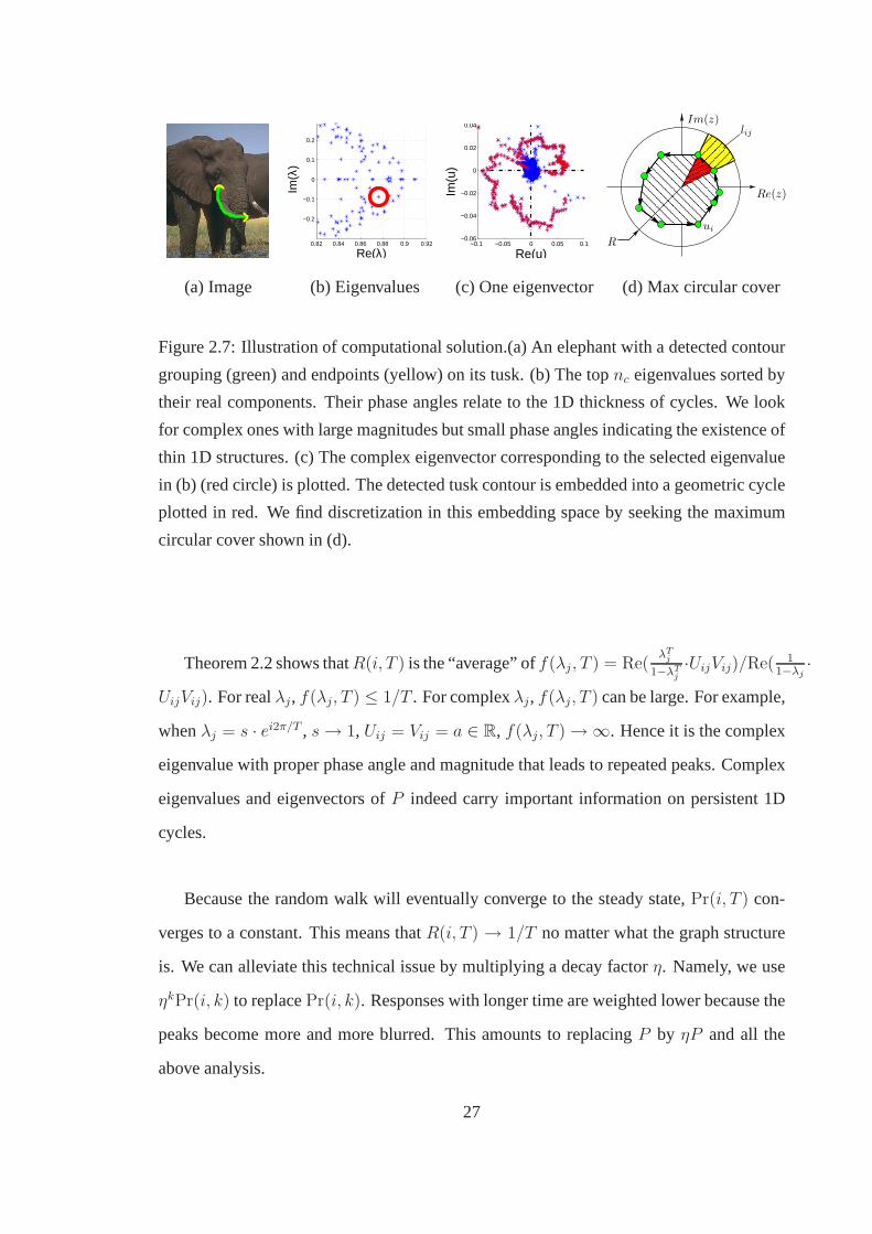
0.82 0.84 0.86 0.88 0.9 0.92

−0.2

−0.1

0

0.1

0.2

0.3

Re(λ)

Im(λ

)

−0.1 −0.05 0 0.05 0.1−0.06

−0.04

−0.02

0

0.02

0.04

Re(u)

Im(u

)

��

��

��

��

��

��

��

��

��

��

��

��

��

��

��

��

��

��

R

ui

Re(z)

Im(z)lij

(a) Image (b) Eigenvalues (c) One eigenvector (d) Max circular cover

Figure 2.7: Illustration of computational solution.(a) Anelephant with a detected contour

grouping (green) and endpoints (yellow) on its tusk. (b) Thetopnc eigenvalues sorted by

their real components. Their phase angles relate to the 1D thickness of cycles. We look

for complex ones with large magnitudes but small phase angles indicating the existence of

thin 1D structures. (c) The complex eigenvector corresponding to the selected eigenvalue

in (b) (red circle) is plotted. The detected tusk contour is embedded into a geometric cycle

plotted in red. We find discretization in this embedding space by seeking the maximum

circular cover shown in (d).

Theorem 2.2 shows thatR(i, T ) is the “average” off(λj , T ) = Re(λT

j

1−λTj

·UijVij)/Re( 11−λj·

UijVij). For realλj, f(λj, T ) ≤ 1/T . For complexλj, f(λj, T ) can be large. For example,

whenλj = s · ei2π/T , s→ 1, Uij = Vij = a ∈ R, f(λj, T )→∞. Hence it is the complex

eigenvalue with proper phase angle and magnitude that leadsto repeated peaks. Complex

eigenvalues and eigenvectors ofP indeed carry important information on persistent 1D

cycles.

Because the random walk will eventually converge to the steady state,Pr(i, T ) con-

verges to a constant. This means thatR(i, T ) → 1/T no matter what the graph structure

is. We can alleviate this technical issue by multiplying a decay factorη. Namely, we use

ηkPr(i, k) to replacePr(i, k). Responses with longer time are weighted lower because the

peaks become more and more blurred. This amounts to replacing P by ηP and all the

above analysis.

27

2.5 Tracing Contours

The complex eigenvector is an approximation of the optimal circular embedding and will

not produce exact 1D cycles. Therefore, we still need to search for 1D cycles in this space.

We will introduce a discretization method and give the overall untangling cycle procedure

in this section.

2.5.1 Discretization

For each of the top complex eigenvectors, we seek discrete topological cycles separated

from the background. First, we can read off the tube size directly from the phase angle of

its corresponding eigenvalue. This determines the “thickness”k of our cycle. Since we

prefer thin 1D cycles, we will only examine top eigenvectorswith small phase angles.

Once knowing the existence of a 1D cycle, we search for it in its complex eigen-

vector whose components arev(1), ...v(2n). The topological graph cycles are mapped

to the geometric cycles in this embedding space. The larger the cycle is geometrically,

the better the 1D graph cycle is topologically. Therefore, we should search for a se-

quences(1), s(2), ..., s(h), s(h + 1) = s(1) such that the re-ordered embedding points

u(1) = v(s(1)), u(2) = v(s(2)), ..., u(h) = v(s(h)) satisfy two criteria: 1) the magni-

tudes|u(1)|, ..., |u(h)| are large and; 2) the phase anglesθ(u(1)), ..., θ(u(h)) are in an

increasing order. This can be tackled by finding the sequenceenclosing the largest area in

the complex plane:

maxs(1),...,s(h)

h∑

j=1

A(u(j), u(j + 1)) (2.22)

HereA(u(j), u(j + 1)) = 12Im(u(j)∗ · u(j + 1)) is the signed area of the triangle spanned

by u(j), u(j + 1) and0.

To accelerate the search, we packu(i) into binsB1, ..., Bm according to their phase

angles. Suppose there is an edge(i, j) in the original graph. Ifu(i) is in a properly

ordered cycle, the phase angle differenceθ(u(j)) − θ(u(i)) will, on average, be equal to

∆θ. Hence, we can safely assume that all its neighborsu(j) are at most one bin apart from

28

u(i) if the bin size is chosen properly (e.g.2∆θ). Furthermore, we group nodes within the

same bin by their spatial connectivity. This greatly reduces the computational cost.

The maximal enclosed area problem can be solved by the shortest path algorithm (see

Fig. 2.7). Notice that the sequenceu(1), ..., u(h), u(h+ 1) = u(1) produces a closed loop

around the origin. Suppose it only wraps around the origin once. For each pair ofi, j in

neighboring bins, setℓij = 12[θ(v(j)) − θ(v(i))] · R2 − A(v(i), v(j)). The numberR is

chosen sufficiently large to guaranteeℓij > 0 for all i,j. Then eq. (2.22) can be reduced to

πR2 − mins(1),...,s(h+1)

h∑

j=1

ℓs(j)s(j+1) (2.23)

This shortest cycle problem can be broken into two parts: thefirst shortest path from

s(1) in bin B1 to a nodes(a) in bin B2, and the second one froms(a) back tos(1). Hence,

the second termmins(1),...,s(h+1)

∑hj=1 ℓs(j)s(j+1) in eq. (2.23) becomes

mins(1)∈B1,s(a)∈B2

s(1),...,s(h+1)

[

a−1∑

j=1

ℓs(j)s(j+1) +

h∑

j=a

ℓs(j)s(j+1)] (2.24)

where each summation itself is a shortest path.

2.5.2 Untangling Cycle Algorithm

In summary, our untangled cycle algorithm has three steps:

Algorithm 1 (Untangling Cycle Algorithm)1: GRAPH SETUP. Construct the directed graphG and compute transition matrixP by

eq. (2.1) and (2.2).

2: COMPLEX EMBEDDING. Compute the firstnc complex eigenvectors ofP . Each

complex eigenvector produces a complex circular embeddingv(1), v(2), ...v(2n) ∈C.

3: CYCLE TRACING. For v(1), v(2), ...v(2n), use shortest path to find a cycleS ⊆

{1, ..., 2n}minimizing (eq. (2.23)).

29

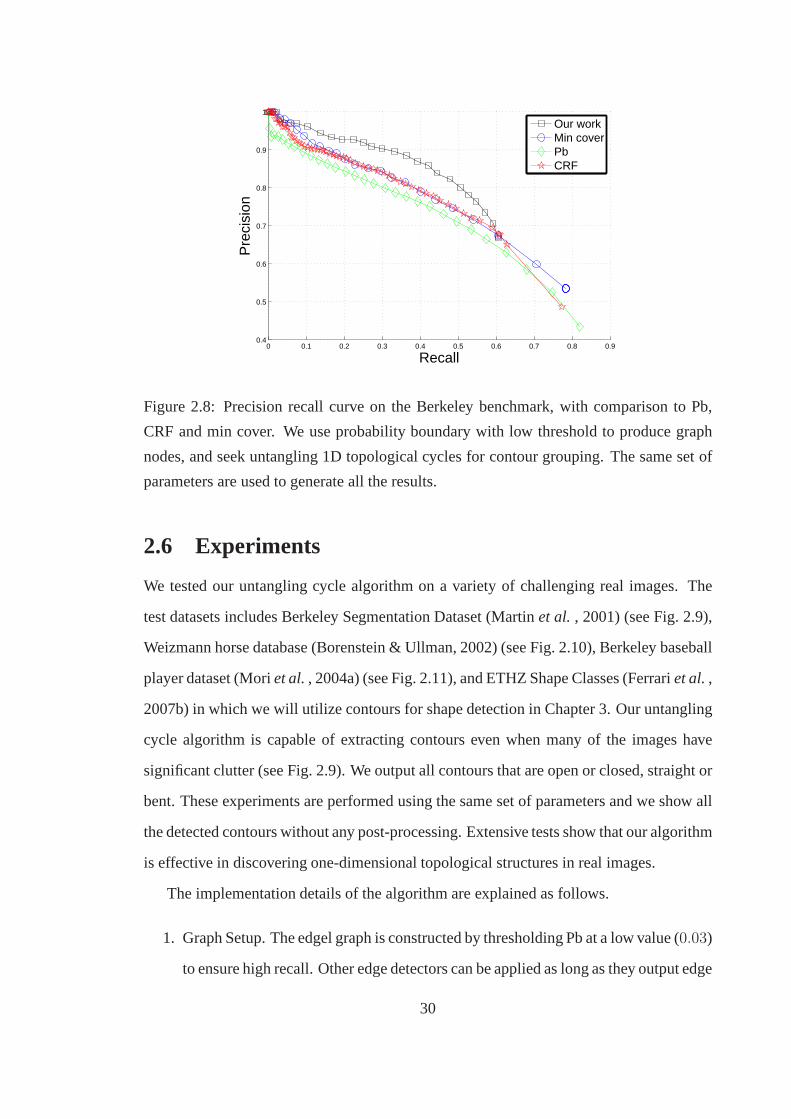
0 0.1 0.2 0.3 0.4 0.5 0.6 0.7 0.8 0.90.4

0.5

0.6

0.7

0.8

0.9

1

Recall

Pre

cisi

on

Our workMin coverPbCRF

Figure 2.8: Precision recall curve on the Berkeley benchmark, with comparison to Pb,

CRF and min cover. We use probability boundary with low threshold to produce graph

nodes, and seek untangling 1D topological cycles for contour grouping. The same set of

parameters are used to generate all the results.

2.6 Experiments

We tested our untangling cycle algorithm on a variety of challenging real images. The

test datasets includes Berkeley Segmentation Dataset (Martin et al. , 2001) (see Fig. 2.9),

Weizmann horse database (Borenstein & Ullman, 2002) (see Fig. 2.10), Berkeley baseball

player dataset (Moriet al., 2004a) (see Fig. 2.11), and ETHZ Shape Classes (Ferrariet al.,

2007b) in which we will utilize contours for shape detectionin Chapter 3. Our untangling

cycle algorithm is capable of extracting contours even whenmany of the images have

significant clutter (see Fig. 2.9). We output all contours that are open or closed, straight or

bent. These experiments are performed using the same set of parameters and we show all

the detected contours without any post-processing. Extensive tests show that our algorithm

is effective in discovering one-dimensional topological structures in real images.

The implementation details of the algorithm are explained as follows.

1. Graph Setup. The edgel graph is constructed by thresholding Pb at a low value (0.03)

to ensure high recall. Other edge detectors can be applied aslong as they output edge

30

tangents/normals. Graph weights are computed within a21× 21 neighborhood for

each edgel.10% of the weights is added to the reverse edges as backward connection

W back to close the open contours in topology. The graph matrix is normalized by

column to generate a random walk matrix.

2. Complex Embedding. We compute200 to 400 eigenvectors of the graph random

walk matrix. The real eigenvectors are pruned because they contain no information

on the contour ordering, as shown in Section 2.4. Eigenvalues whose phase angle is

too large or whose magnitude is too small are also discarded.These indicates bad

cycles with untangling cycle cut score. After eliminating one of the eigenvalue in

each conjugate pair, typically less than 100 eigenvalues/eigenvectors survive.

3. Cycle Tracing. We run the shortest cycle algorithm eq. (2.22) on the embedding

space generated by the remaining eigenvectors. Each complex embedding space is

divided uniformly into8 bins by phase angle. A cycle is broken into two shortest

paths as in eq. (2.24): one from bin1 to bin 2, and the other from bin2 to bin

8 back to bin1. We choose the top 5 cycles in each eigenvector, and combine

the redundant ones. The final output contains partially overlapping contours due

to multiple possibilities at junctions, instead of disjoint contours. These additional

hypotheses are very important for constructing shapes in the next chapter.

The current unoptimized Matlab implementation takes about3 minutes on a300×400 im-

age. The bottleneck of the computation is solving the complex eigenvectors. Similar to the

eigenvalue problem in NCut, techniques of multi-scale graph (Couret al. , 2005) or GPU

implementation (Catanzaroet al. , 2009) can be explored to accelerate the computation in

the future.

Our results are significantly better than those of state-of-the-art, particularly on clut-

tered images. To quantify our performance, we compare our precision-recall curve on

the Berkeley benchmark with two top contour grouping algorithms: CRF (Renet al. ,

2005b) and Min Cover (Felzenszwalb & McAllester, 2006). Ourresults are well above

31

these approaches by about7% in the medium to high precision part (see Fig. 2.8). Visually

our results produce much cleaner contours as shown in Fig. 2.9-2.11. Many of the false

positives are shading edges, which are not labelled by humans. However, once they are

grouped, they could be easily to pruned in later recognitionprocess. These are the advan-

tages not reflected by the metric in the Berkeley benchmark, which counts matched pixels

independently.

2.7 Summary

To our knowledge, this is the first major attack on contour grouping using a topological

formulation. Our grouping criterion of untangling cycles exploits the inherent topological

1D structure of salient contours to extract them from the otherwise 2D image clutter.

We made this precise by defining a directed graph linking local edgels. We encode the

untangling cycle criterion by circular embedding. Computationally, this reduces to finding

the top complex eigenvectors of the random walk matrix. We demonstrate significant

improvements over state-of-the-art approaches on challenging real images.

32

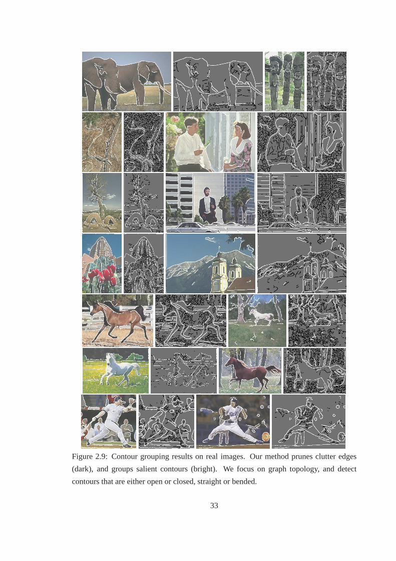
Figure 2.9: Contour grouping results on real images. Our method prunes clutter edges

(dark), and groups salient contours (bright). We focus on graph topology, and detect

contours that are either open or closed, straight or bended.

33

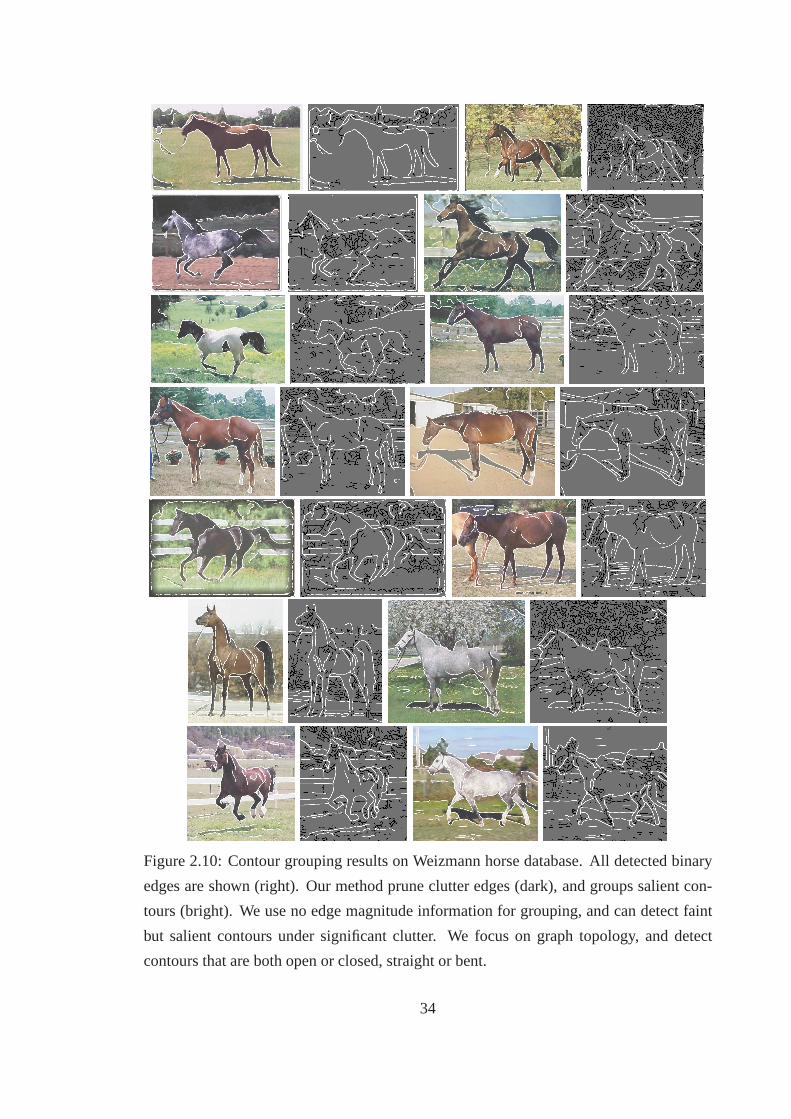
Figure 2.10: Contour grouping results on Weizmann horse database. All detected binary

edges are shown (right). Our method prune clutter edges (dark), and groups salient con-

tours (bright). We use no edge magnitude information for grouping, and can detect faint

but salient contours under significant clutter. We focus on graph topology, and detect

contours that are both open or closed, straight or bent.

34

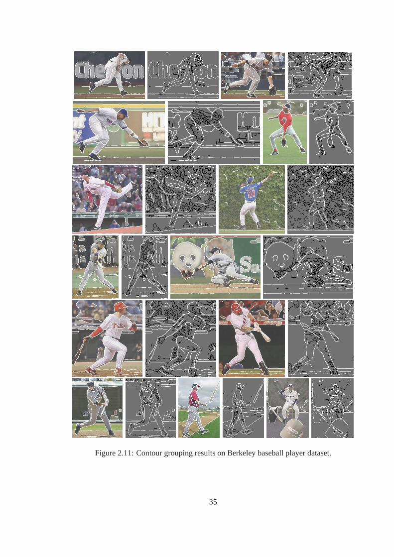
Figure 2.11: Contour grouping results on Berkeley baseballplayer dataset.

35

Chapter 3

Contour Packing

Visual objects can be represented in a variety of levels: from the signal level of filter

responses to the symbolic level of object parts (Ullman, 1996). We focus on the repre-

sentation based on shape that is closer to the symbolic level, allowing abstract geometric

reasoning of objects. Shape-based object description is invariant to color, texture, and

brightness changes, and dramatically reduces the number oftraining examples required,

without sacrificing the detection accuracy.

This chapter presents the contour packing framework that holistically detects and

matches a model shape by packing a set of image contours – an intermediate level of

object representation. We build this framework on top of ourcontour grouping approach

in Chapter 2, which suppresses 2D clutter and produces long topologically 1D contours.

We develop a set-to-set contour matching formulation to bridge the representation gap

between the image and the model due to unpredictable fragmentations of bottom-up con-

tours. The global shape configuration of a contour set is characterized bycontext selective

shape features, constructed from contours within a large spatial context.Unlike traditional

shape features such as (Belongieet al. , 2002) which are precomputed regardless of con-

text changes, context selective shape features adjuston the flydepending on which set of

image contours participate in matching. The generated shape features can be encoded in a

linear form of figure/ground contour selection. This enables the combinatorial search aris-

ing in set-to-set contour matching to be approximated and solved efficiently by an instance

36

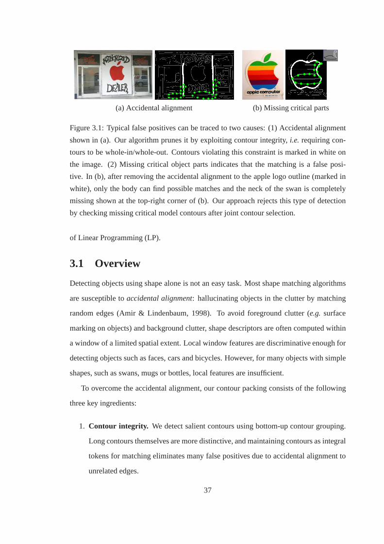
(a) Accidental alignment (b) Missing critical parts

Figure 3.1: Typical false positives can be traced to two causes: (1) Accidental alignment

shown in (a). Our algorithm prunes it by exploiting contour integrity, i.e. requiring con-

tours to be whole-in/whole-out. Contours violating this constraint is marked in white on

the image. (2) Missing critical object parts indicates thatthe matching is a false posi-

tive. In (b), after removing the accidental alignment to theapple logo outline (marked in

white), only the body can find possible matches and the neck ofthe swan is completely

missing shown at the top-right corner of (b). Our approach rejects this type of detection

by checking missing critical model contours after joint contour selection.

of Linear Programming (LP).

3.1 Overview

Detecting objects using shape alone is not an easy task. Mostshape matching algorithms

are susceptible toaccidental alignment: hallucinating objects in the clutter by matching

random edges (Amir & Lindenbaum, 1998). To avoid foregroundclutter (e.g. surface

marking on objects) and background clutter, shape descriptors are often computed within

a window of a limited spatial extent. Local window features are discriminative enough for

detecting objects such as faces, cars and bicycles. However, for many objects with simple

shapes, such as swans, mugs or bottles, local features are insufficient.

To overcome the accidental alignment, our contour packing consists of the following

three key ingredients:

1. Contour integrity. We detect salient contours using bottom-up contour grouping.

Long contours themselves are more distinctive, and maintaining contours as integral

tokens for matching eliminates many false positives due to accidental alignment to

unrelated edges.

37

2. Holistic shape matching. We measure shape features from a large spatial extent,

as well as long-range contextual relationships among object parts. Accidental align-

ment of holistic shape descriptors between image and model is unlikely.

3. Model configuration checking. We break the model shape into its informative

semantic parts, and explicitly check which subset of model parts is matched. Miss-

ing critical model parts can signal an accidental alignmentbetween the image and

model.

We start with salient contours extracted by bottom-up contour grouping in Chapter 2.

Shape matching with contours composed of orderly, grouped edges instead of isolated

edges has several advantages. Long salient contours have more distinctive shapes, which

leads to efficiency of the search as well as the accuracy of shape matching. Furthermore,

by requiring the entire contour to be matched as a whole, we eliminate accidental align-

ment causing false positive detections shown in Fig. 3.1 (a). Using contour grouping as

the starting point of shape matching carries risk as well. Contours could be mis-detected,

or accidentally leaking to background. Therefore, a good contour grouping algorithm is

essential for shape matching. We have demonstrated the goodperformance of our con-

tour grouping algorithm in cluttered images. These contours are not disjoint, providing

multiple hypotheses at junctions where contours can potentially leak to other objects.

The main technical challenge is that image and model contours do not have one-to-

one correspondence. Contours detected from bottom-up grouping and segmentation are

different from the semantically meaningful contours in themodel. However, as a whole

they will have a match (see Fig. 3.2). The holistic matching occurs only by considering a

set of “figure” contours together. To formulate this set-to-set matching task, we introduce

control points sampled on and around image and model contours. We compute shape

features on the control points from the “figure” contours within a large neighborhood (see

Fig. 3.2). The task boils down to finding the correct figure/ground contour selection, such

that there is an optimal one-to-one matching of the control points. The set-to-set matching

potentially requires searching over exponentially many choices of figure/ground selection

38

on contours. We simplify this task by encoding the shape descriptor algebraically in a

linear form of contour selection variables, allowing the efficient optimization technique of

LP.

To evaluate shape matching, one needs to measure the accuracy of alignment, and more

importantly, determinewhichmodel parts have actually been aligned. For simple shapes,

missing a small but critical object part can indicate a complete mismatch (see Fig. 3.1 (b)).

We manually divide the model into contours which corresponds to distinctive parts. Just

as image contours, we require model contours to be whole-in or whole-out.

The rest of the chapter is organized as follows. Section 3.2 introduces the contour

packing formulation and the key concept of context sensitive shape features. We present

the computational solution for this framework using LinearProgramming (LP) in Sec-

tion 3.3. Section 3.4 describes related works and comparisons. Section 3.5 demonstrates

our approach on the challenging task of detecting non-rectangular and wiry shaped ob-

jects, followed by the conclusion in Section 3.6.

3.2 Set-to-Set Contour Matching

In this section we develop the set-to-set contour matching method. The computational

task of set-to-set contour matching consists of parallel searches over image contours and

model contours to obtain the maximal match of the image and model shapes.

3.2.1 Problem Formulation

We start with formulating the shape detection as the following problem:

Definition of set-to-set contour matching.Given an imageI and a modelM represented

by two sets of contours:

• Image:I = {CI1 , C

I2 , . . . C

I|I|}, CI

k is thekth contour;

• Model:M = {CM1 , CM

2 , . . . , CM|M|}, CM

l is thelth contour.

we would like to select the maximal contour subsetsIsel ⊆ I andMsel ⊆ M, such that

object shapes composed byIsel andMsel match (see Fig. 3.2 for an image example).

39

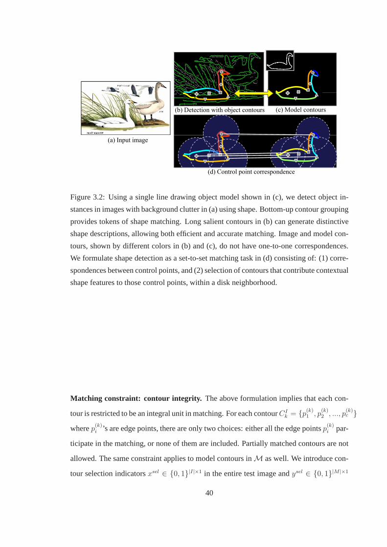
(b) Detection with object contours (c) Model contours

(a) Input image

(d) Control point correspondence

Figure 3.2: Using a single line drawing object model shown in(c), we detect object in-

stances in images with background clutter in (a) using shape. Bottom-up contour grouping

provides tokens of shape matching. Long salient contours in(b) can generate distinctive

shape descriptions, allowing both efficient and accurate matching. Image and model con-

tours, shown by different colors in (b) and (c), do not have one-to-one correspondences.

We formulate shape detection as a set-to-set matching task in (d) consisting of: (1) corre-

spondences between control points, and (2) selection of contours that contribute contextual

shape features to those control points, within a disk neighborhood.

Matching constraint: contour integrity. The above formulation implies that each con-

tour is restricted to be an integral unit in matching. For each contourCIk = {p(k)

1 , p(k)2 , ..., p

(k)c }

wherep(k)i ’s are edge points, there are only two choices: either all theedge pointsp(k)

i par-

ticipate in the matching, or none of them are included. Partially matched contours are not

allowed. The same constraint applies to model contours inM as well. We introduce con-

tour selection indicatorsxsel ∈ {0, 1}|I|×1 in the entire test image andysel ∈ {0, 1}|M |×1

40

in the model defined as

(IMAGE CONTOUR SELECTOR) xselℓ =

1, if contourCI

ℓ is selected

0, otherwise.

(3.1)

(MODEL CONTOUR SELECTOR) yselℓ =

1, if contourCMℓ is selected

0, otherwise.

(3.2)

Control point correspondence. While contours themselves do not correspond one-to-

one, their overall shape configuration can be evaluated at nearby control points, and those

control points do have one-to-one correspondences. Suppose control points{p1, p2, . . . , pm}are sampled from the image and{q1, q2, . . . , qn} are sampled from the model. We define

the correspondence matrix(U cor)m×n from the image to the model as:

U corij =

1, if pi matchesqj

0, otherwise.(3.3)

Note that these control points can be located anywhere in theimage, not limited to contour

points. Computing dense point correspondences is unnecessary. Instead, rough matching

of a few control points is sufficient to select and match contour setsIsel andMsel.

Feature representation: holistic shape features.The important question is, what will

be the appropriate shape feature for matching these controlpoints, and how to compute

shape dissimilarity/distanceDij. In order to be matched, the shape feature has to share a

common description between the image and the model. Since there do not exist one-to-

one correspondences between contours, the feature description is more appropriate on the

contour set or global shape level rather than on the individual contour level. We propose

a holistic shape representation at the control points covering not only nearby contours but

also faraway contours (see Fig. 3.3).

The holistic shape representation immediately poses the problem offigure/ground se-

lection since figure/ground segmentation is unknown and the shape feature is likely to

41

include both foreground and background contours. Without the correct segmentation,

background clutter and contours from other objects can corrupt the shape feature. This

poses great difficulties to any shape features with a fixed context. A fixed context fea-

ture cannot adapt to the combinatorial possibilities of figure/ground selection, with each

generating a different feature. Our strategy is to adjust the context of the holistic shape fea-

tures during matching depending on the figure/ground selection. Therefore, we are able to

compute the right features and determine the figure/ground segmentation simultaneously.

3.2.2 Context Selective Shape Features

We are ready to introduce the holistic shape representationcalled context selective shape

features determined by the figure/ground selection of the contoursxsel andysel. We choose

Shape Contexts (SC) (Belongieet al. , 2002) as the basic shape feature descriptor. Mea-

suring global shape requires the scope of SC to be large enough to cover the entire object.

DefinescIi = [scI

i (1), scIi (2), ..., scI

i (b)]T to be the vector of SC histogram centered at con-

trol point pi, i.e. scIi (k) = # of points in bink. We introduce a contribution matrixV I

i

with size (#bin)×(#contour) to encode the contribution of each contour to each bin ofscIi :

V Ii (k, l) = # of points in bin k from contour Cl (3.4)

Similar notationsscMj andV M

j are defined for SC at control pointqj in the model.

The key observation is that shape featuresscIi will be differentdepending on context

xsel, i.e. they are not fixed. Since each contour can have 2 choices, either selected or not

selected, there exists2n possible contexts – exponential in the number of contoursn. One

advantage of histogram features such as SC is that the exponentially many combinations

of contexts can be written in a simple linear form:

scIi (k) =

∑

l

V Ii (k, l) · xsel

l = (V I · xsel)k (3.5)

This allows us to cast the complex search as an optimization problem later.

Our goal is to findxsel andysel such that they produce similar shape features:V Ii ·

xsel ≈ V Mj · ysel. We evaluate and compare these two features by the context sensitive

42

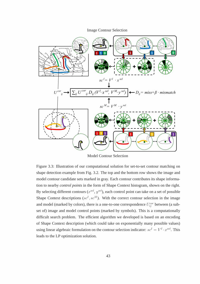
Image Contour Selection

1 1 0

sc I =

�ij Ucor

ij Dij (V I· x seU

corij

Msc M =

1 1 1

1 1 0

V I · x sel

l, V M· y sel)

V M sel

Dij = miss+� · mismatch

= V M · y sel

1 1 1

Model Contour Selection

Figure 3.3: Illustration of our computational solution forset-to-set contour matching on

shape detection example from Fig. 3.2. The top and the bottomrow shows the image and

model contour candidate sets marked in gray. Each contour contributes its shape informa-

tion to nearbycontrol pointsin the form of Shape Context histogram, shown on the right.

By selecting different contours (xsel, ysel), each control point can take on a set of possible

Shape Context descriptions (scI , scM ). With the correct contour selection in the image

and model (marked by colors), there is a one-to-one correspondenceU corij between (a sub-

set of) image and model control points (marked by symbols). This is a computationally

difficult search problem. The efficient algorithm we developed is based on an encoding

of Shape Context description (which could take on exponentially many possible values)

using linear algebraic formulation on the contour selection indicator:scI = V I ·xsel. This

leads to the LP optimization solution.

43

dissimilarity:

(SHAPE DISSIMILARITY ) Dij(scIi , sc

Mj ) = Dij(V

Ii · xsel, V M

j · ysel) (3.6)

The shape dissimilarityDij not only depends on the local attributes ofpi andqj , but more

importantly, on the context given byxsel andysel. Matching object shapes boils down to

minimizingDij , which is a combinatorial search problem onxsel andysel.

3.2.3 Contour Packing Cost

Finding the set-to-set contour matching finally becomes a joint search over correspon-

dencesU cor and contour selectionxsel, ysel by minimizing the following cost:

(Contour Packing Cost)

minUcor,xsel,ysel

Cpacking(Ucor, xsel, ysel) =

1

m

∑

i,j

U corij Dij(V

Ixsel, V Mysel) (3.7)

s.t. U cor ∈ G

wherem =∑

i,j U corij is the number of control point correspondences. Correspondences

U cor from different object parts should have geometric consistency. We use a star model

graph for checking global geometric consistency. Each correspondence(pi, qj) can predict

an object centercij . For the correct set of correspondences, all the predicted centers should

form a cluster,i.e. close to their average center:c(U cor) =∑

cijUcorij wij/

∑U cor

ij wij ,

wherewij ’s are the weights on correspondences. Thus correspondences U cor satisfying

the geometric consistency constraint can be expressed as:

(GEOMETRIC CONSISTENCY) G = {‖c(U cor)− cijUcorij ‖ ≤ dmax if U cor

ij = 1}

(3.8)

wheredmax is the maximum distance allowed for deviation from the center.

44

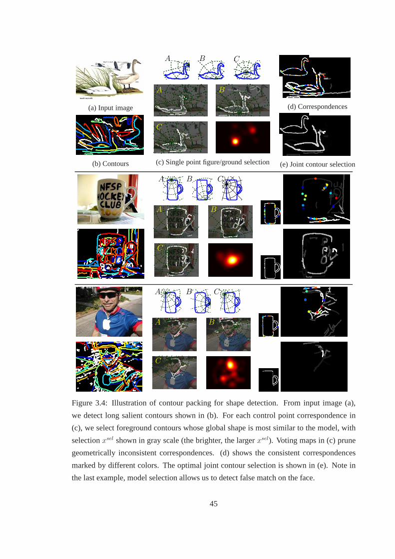
(a) Input image

(b) Contours

A B C

A B

C

(c) Single point figure/ground selection

(d) Correspondences

(e) Joint contour selection

A B C

A B

C

A B C

A B

C

Figure 3.4: Illustration of contour packing for shape detection. From input image (a),

we detect long salient contours shown in (b). For each control point correspondence in

(c), we select foreground contours whose global shape is most similar to the model, with

selectionxsel shown in gray scale (the brighter, the largerxsel). Voting maps in (c) prune

geometrically inconsistent correspondences. (d) shows the consistent correspondences

marked by different colors. The optimal joint contour selection is shown in (e). Note in

the last example, model selection allows us to detect false match on the face.

45

3.3 Computational Solution via Linear Programming

Direct optimization of contour packing cost function eq. (3.7) is a hard combinatorial

search problem. The shape dissimilarityDij(VI · xsel, V M · ysel) can only be evaluated

given correspondencesU cor. However, finding the correct correspondencesU cor requires

xsel andysel. Therefore, the inference problem becomes circular. We approximate this

joint optimization by breaking the loop into two steps:single point figure/ground selec-

tion and joint contour selection(see Fig. 3.4). The first step focuses on finding reliable

correspondencesU cor (maybe sparse) by matching image contours to the whole model.

Note that even this subroutine is a combinatorial search, with exponentially many combi-

nations of figure/ground selection. The second step selectscontours simultaneously from

both image contours labelled as figure and all the model contours being matched, based

on the correspondences computed in the first step. This section presents the relaxation of

both steps as an instance of Linear Programming (LP).

3.3.1 Single Point Figure/Ground Selection

Our first step discovers all potential control point correspondencesUij and computes the

corresponding figure/ground selectionxsel for them. We fixysel = 1 to encourage match-

ing to the full model as much as possible. In this step, partial matches are undesired since

the correspondences they produce are much less reliable. Weuse the simpleL1-norm as

the dissimilarityDij . Accordingly, the contour packing cost eq. (3.16) reduces the the

following problem:

minxsel

‖V I · xsel − V M · ysel‖1, xsel ∈ {0, 1}|I| (3.9)

A brute force approach of the above problem is formidable even for mid-size problems

with 20 to 30 contours. We compute an approximate solution by relaxing the binary vari-

ablesxsel to continuous values:0 ≤ xsel ≤ 1. Since the norm in the cost function isL11.

1BesidesL1, other distance functions such asL2 andχ2 for shape context can also be used. However,the relaxations will be computationally much more intensive. We will see discussion onL2 in later thissection and Appendix.

46

By introducing slack variablesb+, b− ≥ 0 such thatV I · xsel − V M · ysel = b+ − b−, we

can reduce the problem to a standard LP:

(CONTOUR PACKING LP) minxsel,b+,b−

1Tb+ + 1Tb− (3.10)

s.t. V Ixsel − V Mysel = b+ − b−

0 ≤ xsel ≤ 1

b+, b− ≥ 0

This LP problem can be solved efficiently by off-the-self LP solvers such as Mosek (An-

dersen & Andersen, 2000). We will see even more efficient solutions using primal-dual

algorithms in the next chapter.

L2-norm Dissimilarity: A MaxCut Approach

The choice of shape dissimilarityDij has a significant impact on solving the com-

binatorial problem of contour packing. One alternative to theL1-norm used in eq. (3.9)

is to haveL2-norm: ‖V I · xsel − V M · ysel‖2. We have discovered that this can be re-

duced to MaxCut, with a proved bound on approximation via Semidefinite Programming

(SDP) (Goemans & Williamson, 1995). The derivation of this connection is summarized

in following theorem:

Theorem 3.1. Construct a graphGpacking = (V, E, W ) with V = I ∪ M ∪ A and

wij = aTi aj, where

ai =

V I(:,i) if nodei ∈ I

V M(:,i) if nodei ∈M

(0, ..., 0, |∑k V Iik −

∑k V M

ik |, 0, ..., 0)T if nodei ∈ A

(3.11)

Here V I(k, i) is the feature contribution of contouri to the histogram bink defined in

eq. (3.4). VectorsV I(:,i) andV M

(:,i) represents theith columns ofV I andV M .

The optimal subsetSI∗ andSM

∗ with the best matching cost‖V I · xsel − V M · ysel‖2 is

given by the maximum cut of the graphGpacking. If (C1, C2) is the cut withV0 ∈ C2, the

optimal subsets are given bySI∗ = I ∩ C1 andSM

∗ =M∩ C2.

47

Proof. Please see Appendix.

Although the relaxation of SDP provides a tighter approximation in theory,L2-norm

is not as goodL1-norm as a distance function for feature description.L2-norm is sus-

ceptible to large values in the histogram bins, and hence less robust to image outliers and

noises. Therefore, theL1-norm dissimilarity and the LP relaxation is adopted in the subse-

quent sections. We will revisit the SDP relaxation in Chapter 6, which provides additional

expressive power for region packing.

Correspondences found from single point figure/ground selection might not satisfy

geometric consistency eq. (3.8). Therefore, we enforce geometric consistency by pruning

hypotheses of control point correspondences via a voting procedure (Wanget al. , 2007).

Each image control point can predict an object center using its best match to model con-

trol points computed by eq. (3.9). These predictions generate votes weighted by the shape

dissimilarity, and accumulates to a voting map. We extract object centers from the local

maxima and further back-trace the voters to identify geometrically consistent correspon-

dences.

3.3.2 Joint Contour Selection

Once obtaining a group of geometrically consistent correspondences, we seek a subset

of contours that match well consistently across all correspondences in eq. (3.7). In single

point figure/ground selection, the selected contours at different control points are not guar-

anteed to be the same. The shape feature centered at each control point essentially covers

the whole object. However, the sensitivity of shape description differs: close-by shape

descriptions are more precise to be discriminative, and thefaraway ones are more blurry

to tolerate deformations. A unification of these descriptions from different control points

can generate an overview of the shape without losing the details. Given a list of con-

trol point correspondences(i(1), j(1)), (i(2), j(2)), ..., (i(k), j(k)) whereU cori(s),j(s) = 1,

we can stack the all the contribution matrices for image contours into one matrix, and

48

similarly for the model side:

V I =

V Ii(1)

V Ii(2)

...

V Ii(k)

, V M =

V Ij(1)

V Ij(2)

...

V Ij(k)

(3.12)

The contour packing cost in eq. (3.7) can be written in the following matrix form:

k∑

s=1

‖V Ii(s) · xsel − V M

j(s) · ysel‖1 = ‖V I · xsel − V M · ysel‖1 (3.13)

Note that this is an optimization problem with exactly the same form as eq. (3.9). There-

fore the previous LP-based computational solution appliesdirectly.

Maximal matching cost. Recall that our problem is to search for the maximal common

subsets from the image and model contours such that their shapes are similar.What is the

right matching costDij(VIi · xsel, V M

j · ysel) that can enforce the maximal condition?. A

straightforward cost function, such as theL1-norm used previously:Dij(VIi · xsel, V M

j ·ysel) = ‖V I

i · xsel − V Mj · ysel‖, will simply result in the trivial solution which chooses

empty sets from both sides (i.e. xsel = 0, ysel = 0). In fact all the norms as well as

χ2 distance will suffer from the same problem. We introduces the maximal matching

cost for Dij which balances the maximal requirement on the contour selection and the

quality of the match. We seek to match as many model contours as possible while the

difference between image and model contours is small. Before describing the details, we

first introduce a few variables. Set

• scMFj = V M

j yfull to be the shape context centered at model pointqj selecting the

full model, whereyfull = 1|M| means selecting all model contours;

• scIi = V I

i xsel to be the shape context with selectionxsel on image atpi;

• scMj = V M

j ysel to be the shape context with selectionysel on model atqj .

We usescMFj (k), scI

i (k), scMj (k) to denote thekth bin in the shape context.

49

Our maximal matching cost consists of two terms:missandmismatch(see Fig. 3.3).

To match as many model contours as possible, the following difference between the num-

ber of matched points and that of full model points should be minimized:

miss(ij)k = scMF

j (k)−min(scIi (k), scM

j (k)) (3.14)

Heremin(scIi (k), scM

j (k)) counts the number of matched contour points between the im-

age and model in shape context bink.

The above termmiss(ij)k alone does not measure how well the selected image contours

match to the selected model contours. To ensure the matchingquality, the amount of

difference between the number of image and model contour points in all shape context

bins needs to be minimized:

mismatch(ij)k = |scI

i (k)− scMj (k)| (3.15)

By combining eq. (3.14) and eq. (3.15), we have the followingdissimilarity:

Dij =

∑k[miss

(ij)k + β ·mismatch

(ij)k ]∑

k scMFj (k)

(3.16)

whereβ > 1 is a factor balancing the two types of costs. We use∑

k scMFj (k) to normalize

the costDij such that it is invariant to the number of contour points.

LP can also be used to solve eq. (3.7) for contour context selection by relaxingxsel

andysel to real value vectors. eq. (3.16) and eq. (3.7) translate to the following problem:

minxsel,ysel

∑

Ucorij =1

{ 1

Ni

∑

k

[scMFi (k)−min(scI

i (k), scMj (k))] +

β

Ni

‖scIi − scM

j ‖1}

s.t. scIi = V I

i · xsel, scMj = V M

j · ysel

whereNi =∑

k scMFi (k) is a normalization constant andmin(x, y) computes the element-

wise min of vectorsx andy. The two terms in the summation aremiss andmismatch in

eq. (3.16) respectively. The above problem can be relaxed toan instance of LP by adding

slack variablessijk ≥ scIi (k) andsijk ≥ scM

j (k) for min(scIi (k), scM

j (k)).

We have obtained the rough correspondencesU cor from the previous step. We opti-

mize the contour selection cost eq. (3.7)w.r.t. xsel, ysel to prune false positives and detect

50

objects. The outcome includes both the matching costCpacking and model contours actu-

ally matched, indicated byysel. Both of them can be used to prune false positives. Note

that it is not required to have a complete correspondence setU cor since the cost eq. (3.16)

has been normalized by the number of correspondences.

Model configuration checking. The selected model contours from joint contour selec-

tion form a shape configuration that are actually matched to image contours. Because the

number of object model contours is typically very limited (usually 6 to 8), we can specify

a dictionary of all possible configurations of true positives. Detection of model contours

with bad configurations, e.g. missing critical parts, are rejected. This configuration check-

ing together with the matching costCpacking can prune most of the false positives while

preserving true positives. The last row in Fig. 3.4 shows such a case.

3.4 Related Work and Discussion

Salient contours and their configurations are more distinctive than individual edge points

for shape matching. The works (Ferrariet al. , 2007b; Ferrariet al. , 2007a) represent

objects by learning a codebook of Pairs of Adjacent Segments, which are consecutive

roughly straight contour fragments. They achieve detection using a bag-of-words ap-

proach. In (Shottonet al. , 2005), boosted contour-based shape features are learned for

object detection. These efforts utilize mostly short contour fragments, and therefore have

to rely on many training examples to boost the discriminative power of shape features. In

contrast, our work takes the advantage of contour grouping such as (Zhuet al. , 2007)

to detect long salient contours, capturing more global geometric information of objects.

More importantly, we constrain these long contours to act asa whole unit,i.e. they can

either be entirely matched to an object, or entirely belong to the background. This char-

acteristic makes shape matching more immune to accidental alignment to background

clutter. Similar properties are exploited by grouping-based verification approaches (Amir

& Lindenbaum, 1998), and the recent work (Felzenszwalb & Schwartz, 2007).

From a broader perspective, our recognition framework is based on shape matching,

51

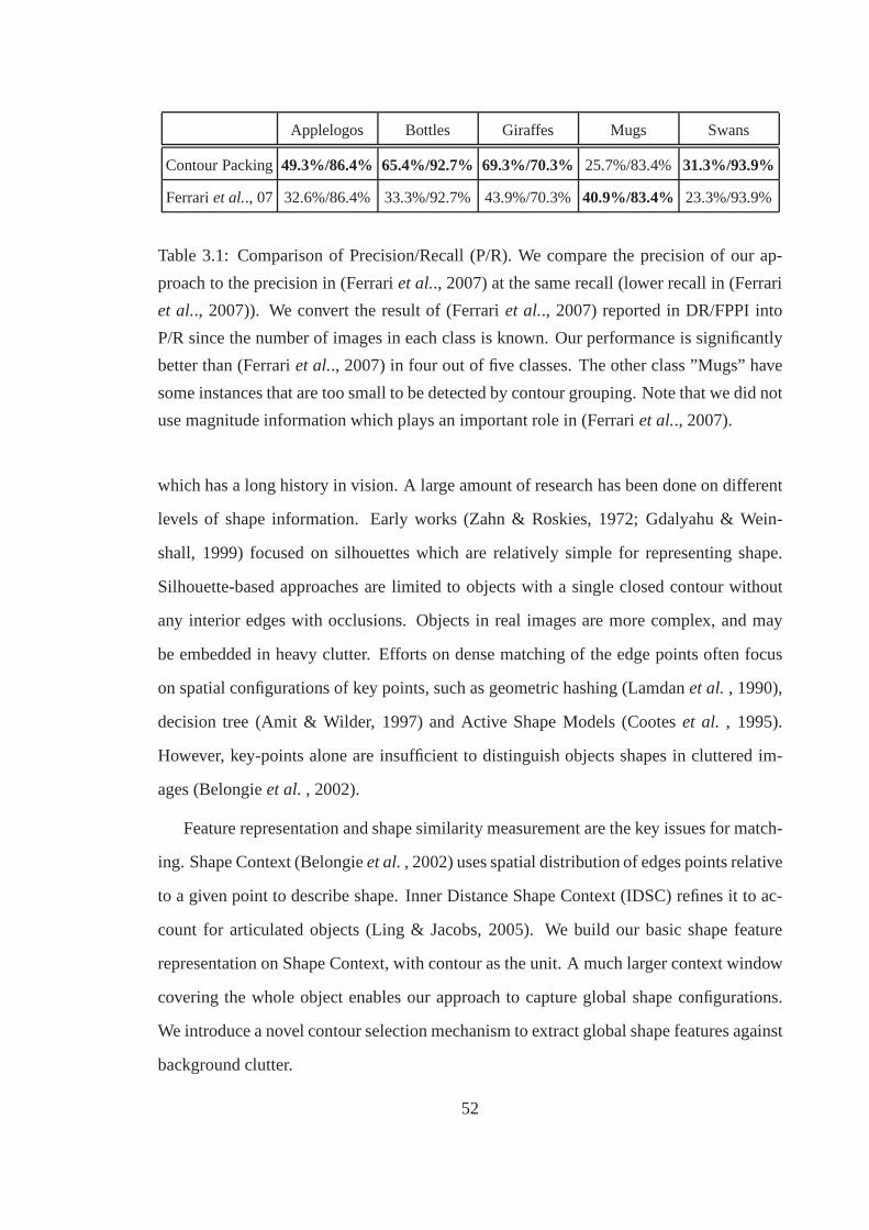
Applelogos Bottles Giraffes Mugs Swans

Contour Packing49.3%/86.4% 65.4%/92.7% 69.3%/70.3% 25.7%/83.4% 31.3%/93.9%

Ferrariet al.., 07 32.6%/86.4% 33.3%/92.7% 43.9%/70.3% 40.9%/83.4% 23.3%/93.9%

Table 3.1: Comparison of Precision/Recall (P/R). We compare the precision of our ap-

proach to the precision in (Ferrariet al.., 2007) at the same recall (lower recall in (Ferrari

et al.., 2007)). We convert the result of (Ferrariet al.., 2007) reported in DR/FPPI into

P/R since the number of images in each class is known. Our performance is significantly

better than (Ferrariet al.., 2007) in four out of five classes. The other class ”Mugs” have

some instances that are too small to be detected by contour grouping. Note that we did not

use magnitude information which plays an important role in (Ferrariet al.., 2007).

which has a long history in vision. A large amount of researchhas been done on different

levels of shape information. Early works (Zahn & Roskies, 1972; Gdalyahu & Wein-

shall, 1999) focused on silhouettes which are relatively simple for representing shape.

Silhouette-based approaches are limited to objects with a single closed contour without

any interior edges with occlusions. Objects in real images are more complex, and may

be embedded in heavy clutter. Efforts on dense matching of the edge points often focus

on spatial configurations of key points, such as geometric hashing (Lamdanet al. , 1990),

decision tree (Amit & Wilder, 1997) and Active Shape Models (Cooteset al. , 1995).

However, key-points alone are insufficient to distinguish objects shapes in cluttered im-

ages (Belongieet al. , 2002).

Feature representation and shape similarity measurement are the key issues for match-

ing. Shape Context (Belongieet al., 2002) uses spatial distribution of edges points relative

to a given point to describe shape. Inner Distance Shape Context (IDSC) refines it to ac-

count for articulated objects (Ling & Jacobs, 2005). We build our basic shape feature

representation on Shape Context, with contour as the unit. Amuch larger context window

covering the whole object enables our approach to capture global shape configurations.

We introduce a novel contour selection mechanism to extractglobal shape features against

background clutter.

52

3.5 Experiments

We demonstrate our detection approach using only one hand-drawn model without nega-

tive training images, To evaluate our performance, we choose the challenging ETHZ Shape

Classes (Ferrariet al., 2007a) containing five diverse object categories with 255 images in

total. Each image has one or more object instances. All categories have significant scale

variances, illumination changes and intra-class variations. Moreover, many objects are

surrounded by extensive background clutter and have interior surface markings. We have

the same experimental setup as (Ferrariet al. , 2007a), using only a single hand-drawn

model for each class and all 255 images as test set. To adapt tolarge scale variance, we

resize the model in 5 to 8 scales with a ratio step of1.3 for each class.

We first use contour grouping developed in Chapter 2 to generate long salient contours

from images. Contours can have overlaps due to multiple possible groupings at junctions.

The Shape Context (SC) used for contour selection covers theentire model shape with a

large spatial extent. The SC histogram has 12 polar bins, 5 radial bins and 4 edge orien-

tation bins. To tolerate shape deformation and eliminate the border artifact of histogram

binning, bin counts are blurred as in (Wanget al. , 2007). This refinement can be encoded

into contribution matricesV I , V M as well.

We sample control point hypotheses on image contours uniformly with an interval

equal to1/10 of the model bounding box diagonal. The number of image control points

sampled in each scale ranges from50 to 400. The numbers of model control points vary

from 15 to 30 depending on the complexity of the target shape. LPs arisingfrom single

point figure/ground selection as well as joint contour selection are solved by the interior

point method. The computation time for each hypothesized correspondence in single point

figure/ground selection is within 0.1 sec.

After selecting figure contours, each correspondence votesfor the object center with

the weight inversely proportional to the shape matching cost. We collect the votes into

a voting map and extract its local maxima above certain threshold to generate object hy-

potheses. Since the correct object scale is unknown beforehand, voting is performed in a

53

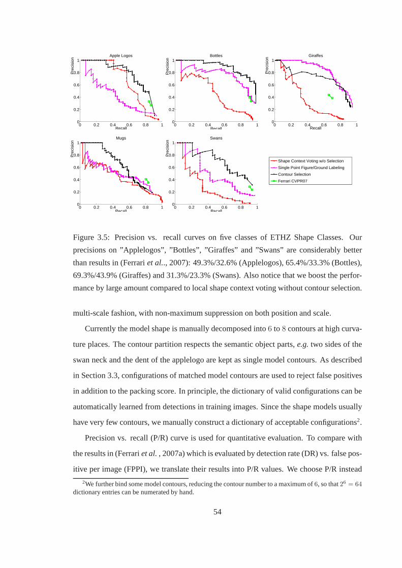
0 0.2 0.4 0.6 0.8 10

0.2

0.4

0.6

0.8

1

Recall

Pre

cisi

on

Apple Logos

0 0.2 0.4 0.6 0.8 10

0.2

0.4

0.6

0.8

1

Recall

Pre

cisi

on

Bottles

0 0.2 0.4 0.6 0.8 10

0.2

0.4

0.6

0.8

1

Recall

Pre

cisi

on

Giraffes

0 0.2 0.4 0.6 0.8 10

0.2

0.4

0.6

0.8

1

Recall

Pre

cisi

on

Mugs

0 0.2 0.4 0.6 0.8 10

0.2

0.4

0.6

0.8

1

Recall

Pre

cisi

on

Swans

Shape Context Voting w/o Selection

Single Point Figure/Ground Labeling

Contour Selection

Ferrari CVPR07

Figure 3.5: Precision vs. recall curves on five classes of ETHZ Shape Classes. Our

precisions on ”Applelogos”, ”Bottles”, ”Giraffes” and ”Swans” are considerably better

than results in (Ferrariet al.., 2007): 49.3%/32.6% (Applelogos), 65.4%/33.3% (Bottles),

69.3%/43.9% (Giraffes) and 31.3%/23.3% (Swans). Also notice that we boost the perfor-

mance by large amount compared to local shape context votingwithout contour selection.

multi-scale fashion, with non-maximum suppression on bothposition and scale.

Currently the model shape is manually decomposed into6 to 8 contours at high curva-

ture places. The contour partition respects the semantic object parts,e.g.two sides of the

swan neck and the dent of the applelogo are kept as single model contours. As described

in Section 3.3, configurations of matched model contours areused to reject false positives

in addition to the packing score. In principle, the dictionary of valid configurations can be

automatically learned from detections in training images.Since the shape models usually

have very few contours, we manually construct a dictionary of acceptable configurations2.

Precision vs. recall (P/R) curve is used for quantitative evaluation. To compare with

the results in (Ferrariet al., 2007a) which is evaluated by detection rate (DR) vs. false pos-

itive per image (FPPI), we translate their results into P/R values. We choose P/R instead

2We further bind some model contours, reducing the contour number to a maximum of6, so that26 = 64dictionary entries can be numerated by hand.

54

of DR/FPPI because DR/FPPI depends on the ratio of the numberof positive and negative

test images and hence is biased. Our final results on this dataset can be seen in Fig. 3.5.

Results of the two steps of our framework are both evaluated.Single point figure/ground

labeling only uses matching cost as the final evaluation for detection, while joint con-

tour selection uses both matching cost and the detected shape configuration. Compared to

the latest result in (Ferrariet al. , 2007a), our performance is considerably better on four

classes out of five. We also compare voting using simple localshape context with our first

step of contour selection. Contour selection greatly improves detection performances (see

Fig. 3.5).

Our shape matching algorithm can reliably extract and select contours of object in-

stances in test images, robust to background clutter and missing contours. Image results

of detection with selected object and model contours are demonstrated in Fig. 3.6.

3.6 Summary

We have introduced a novel shape-based recognition framework calledContour Packing.

We construct context sensitive shape features depending onselected contours and propose

a method to search for the best match. Joint selection on bothimage and model contours

ensures detection to be robust to background clutter and accidental alignment. We are able

to detect object in cluttered images using only one trainingexample. Experiments on hard

object detection task demonstrate promising results.

55

67.04 67.91 51.20 44.35 0.00 52.40

34.72 46.64 47.66 16.04 36.89 19.90

60.26 48.20 69.20 0.00 0.00 56.24

54.71 43.65 45.20 62.28 51.26

70.67 72.32 56.59 55.07 19.64

84.04 64.76 73.11 94.74 67.33 67.03

False positives pruned by model contour selection Failure cases

Figure 3.6: Examples of contour context selection on model and image contours in ETHZ

Shape Classes. The first five rows show detected objects from image with significant

background clutter. In the last row, the first four cases are false positives successfully

pruned by our algorithm by checking the configurations of selected model contours. The

last two are failure cases. Each image only displays one detected object instance.

56

Chapter 4

The Primal-Dual Packing Algorithm

In the previous chapter, we developed the set-to-set contour matching framework and de-

rived a computational solution based on LP. The core of the solution is to encode the

overall shapes at several control points in a linear form of figure/ground contour selec-

tion, which do have one-to-one correspondences. Since the control point correspondences

are unknown, searching for the correct ones results in many LPs, one for each correspon-

dence hypothesis. A natural question arises: do we really need to solve all LPs for the

figure/ground contour selection precisely?

This chapter will show that this is unnecessary for most of the time. We introduce

primal-dual combinatorial algorithms which have generated fast algorithms for a large

class of packing and covering problems. The contour packingLP can be reduced to a bin

covering LP, where these primal-dual ideas can be readily applied. By exploiting the dual-

ity between contours and feature bins, the algorithm is ableto either find an approximate

solution, or declare a lower bound on the optimum of the cost function. Therefore, most

suboptimal solutions can be knocked out without running theLP to the end. Each itera-

tion of the primal-dual algorithm only involves a simple operation of sorting the contours,

making it very fast to generate approximate solutions.

57

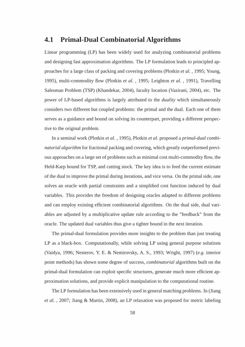
4.1 Primal-Dual Combinatorial Algorithms

Linear programming (LP) has been widely used for analyzing combinatorial problems

and designing fast approximation algorithms. The LP formulation leads to principled ap-

proaches for a large class of packing and covering problems (Plotkinet al. , 1995; Young,

1995), multi-commodity flow (Plotkinet al. , 1995; Leightonet al. , 1991), Travelling

Salesman Problem (TSP) (Khandekar, 2004), faculty location (Vazirani, 2004), etc. The

power of LP-based algorithms is largely attributed to theduality which simultaneously

considers two different but coupled problems: the primal and the dual. Each one of them

serves as a guidance and bound on solving its counterpart, providing a different perspec-

tive to the original problem.

In a seminal work (Plotkinet al. , 1995), Plotkinet al.proposed aprimal-dual combi-

natorial algorithmfor fractional packing and covering, which greatly outperformed previ-

ous approaches on a large set of problems such as minimal costmulti-commodity flow, the

Held-Karp bound for TSP, and cutting stock. The key idea is tofeed the current estimate

of the dual to improve the primal during iterations, and viceversa. On the primal side, one

solves an oracle with partial constraints and a simplified cost function induced by dual

variables. This provides the freedom of designing oracles adapted to different problems

and can employ existing efficient combinatorial algorithms. On the dual side, dual vari-

ables are adjusted by a multiplicative update rule according to the ”feedback” from the

oracle. The updated dual variables thus give a tighter boundin the next iteration.

The primal-dual formulation provides more insights to the problem than just treating

LP as a black-box. Computationally, while solving LP using general purpose solutions

(Vaidya, 1996; Nesterov, Y. E. & Nemirovsky, A. S., 1993; Wright, 1997) (e.g. interior

point methods) has shown some degree of success,combinatorialalgorithms built on the

primal-dual formulation can exploit specific structures, generate much more efficient ap-

proximation solutions, and provide explicit manipulationto the computational routine.

The LP formulation has been extensively used in general matching problems. In (Jiang

et al. , 2007; Jiang & Martin, 2008), an LP relaxation was proposed for metric labeling

58

with L1-norm regularization in image matching. A simplex-based solution and an effi-

cient successive convexification implementation were developed. Alternatively, interior

point method was applied in a related formulation in image registration (Taylor & Bhus-

nurmath, 2008). The structure of the problem was exploited more effectively in solving

the linear systems using specific matrix structures. LP was also used in the inner loop

of iterative algorithms of Integer Quadratic Programming (IQP) arising in matching (Ren

et al. , 2005a; Berget al. , 2005). Although also formulated as an LP, our problem dif-

fers from previous ones in that set-to-set matching insteadof one-to-one correspondence

on feature points is performed. The selection variables in set-to-set matching are more

densely related to each other, resulting in a fundamentallydifferent matrix structure.

The rest of this chapter is organized as follows. Section 4.2will review primal-dual

algorithms for general fractional packing and covering problems, and lay down the founda-

tion for applying these ideas subsequently in the contour packing problem. In Section 4.3

we reduce the single point figure/ground selection LP to a covering problem, and pro-

pose a primal-dual algorithm that enables pruning suboptimal solutions early. Section 4.4

describes details of how to apply the algorithm to contour packing.

4.2 Primal-Dual Algorithms for Packing and Covering

The packing problem studies how to optimally fill a knapsack by choosing the most valu-

able objects from a list. Suppose there aren objects whose prices arepi (i = 1, ..., n).

One would like to choose a subset of these items maximizing their total price, subject to

m capacity constraints such as weight, dimension, etc. Denote the maximum value of

each capacity constraint ascj and the contribution from itemi asWji. Finding the optimal

packing can be written as the following integer programmingproblem:

(PACKING IP) maxx∈{0,1}n

∑

i

pixi

s.t.∑

i

Wjixi ≤ cj , j = 1, ..., m (4.1)

59

wherexi is the 0/1 indicator of whether objecti is selected. By relaxing the integer

constraintx ∈ {0, 1}n to 0 ≤ x ≤ 1, we obtain a linear program calledfractional packing

which provides a lower bound to eq. (4.2):

(PACKING LP) maxx∈Rn

pTx (4.2)

s.t. A · x ≤ c, x ≥ 0

HereA = [W ; I] and c = [c1, ..., cm, 1, ..., 1︸︷︷︸n

]T. Hence the constraintx ≤ 1 has been

folded into the matrix constraintA · x ≤ c.

The covering problem is to find sets with minimal total cost tocover elements. Let the

cj ’s be the costs of then sets. Each setj covers elementi for Wij times. The multiplicity

of each elementi to be covered is required to be at leastpi. Let yj be the number of copies

of setj that are selected (choosing multiple copies are allowed). Similarly to packing, the

covering problem can be written as an integer program, and relaxed tofractional covering:

(COVERING IP) miny∈Nn

∑

j

ciyj (4.3)

s.t.∑

j

Wijyj ≥ pi, i = 1, ..., n

(COVERING LP) miny∈Rn

cTy (4.4)

s.t. AT · y ≥ p, y ≥ 0

The fractional packing problem eq. (4.2) and fractional covering eq. (4.4) are actu-

ally Lagrangian duals. By introducing nonnegative Lagrangian multipliers(y, λ) to the

constraintsA · x ≤ c and x ≥ 0 respectively, the Lagrangian functionL(x, y, λ) =

pTx + yT(c− Ax) + λTx always serves as an upper bound of the fractional packing cost

functionpTx, wheneverx is feasible or not. Therefore,maxx L(x, y, λ) bounds the op-

timum of eq. (4.2). By strong duality of linear program, the optimum of eq. (4.2) and

eq. (4.4) coincides (Boyd & Vandenberghe, 2004). Thereforepacking and covering are

essentially flipped sides of the same coin: solving one implies the other.

Primal and dual formulations provide different perspectives on the problem: for the

feasibility version, primal solution serves as “yes” certificate while the dual solution serves

60

as “no” certificate. Just as the divide-and-conquer strategy, one would like to generate a

series of yes and no certificates to narrow down the search space. Therefore, primal and

dual need to communicate, and use one to update the other.

We start with a feasibility version of the fractional packing problem:

(Feasibility Problem) Given a convex setP ⊆ Rn, anm× n constraint matrixA

and ann× 1 vectorc, determine whether there existsx ∈ P such that

aTj x− cj ≤ 0, j = 1, ..., m (4.5)

HereaTj is thejth row of matrixA.

For the packing problem (4.2), the convex setP is a simple polytope:

P = {x : pTx ≥ α, 0 ≤ x ≤ 1} (4.6)

whereα is a constant. If eq. (4.5) is feasible, then the optimal value µ∗p of eq. (4.2) is

at leastα. Otherwise it is less thanα. By a binary search onα, one can find a(1 + β)

approximation to the optimization problem withinO(log β). Our discussion will focus on

eq. (4.5) in the subsequent sections.

4.2.1 Multiplicative Weight Update: From Primal to Dual

Suppose we are given a primal estimate and its correspondingcost as feedback, how can

we update the current dual estimate? We start with considering an online prediction prob-

lem.

Online Prediction. There arem experts who make predictions on uncertain events in

the world. Our goal is to construct the best strategy over time from these experts. At

time t (t = 0, 1, 2, ...), if the prediction from thejth expert is taken, the event (possibly

adversarial) incurs a positiverewardRtj and a negativeloss−Lt

j. Hence the netvalue

gained isV tj = Rt

j − Ltj. One can construct a mixed strategy from these experts by

linearly combining their predictions. A mixed strategy specifies positives weightsyt =

(y1, ..., ym)T on all the experts. The total net value of the strategy will beV t =∑

j ytjV t

j

61

whereyt = yt/∑

j ytj are the normalized weights. Consider the event sequence from time

t = 0 to T . At time t, the strategy chooses weightsyt on the experts based on all previous

observationsRk andLk with 0 ≤ k ≤ t − 1, and gains a valueV t. One would like to

maximize the cumulative value over timeV =∑T

t=0 V t.

Intuitively, experts making correct predictions previously should be up-weighted while

experts predicting incorrectly should be down-weighted. In other words, the weights

should be updated according to the “feedback” of the expertsfrom the worldV tj . We

introduce a multiplicative weight update scheme to guide the strategy from the feedback:

(Multiplicative Weight Update) Initialize weightsy(0) = (1, ..., 1)T. At time

t, prediction from expertj produces a value ofV tj ∈ [−1, 1]. Given a constant

ǫ ∈ (0, 1), update the weightsyt+1 at timet + 1 by

yt+1j = yt

j exp(ǫV tj) (4.7)

Theorem 4.1. (Littlestone & Warmuth, 1989) (Perturbed Value of the Strategy) LetR =∑

t

∑j yt

jRtj andL =

∑t

∑j yt

jLtj be the cumulative reward and loss of the strategy

using eq. (4.7). The perturbed value of the strategy given byeq. (4.7) is worse than the

performance of best pure strategy only bylog mǫ

, as stated in the following inequality:

maxjVj ≤ exp(ǫ)R− exp(−ǫ)L+

log m

ǫ(4.8)


Theorem 4.1 is essential in the complexity analysis in the subsequent sections. It

proves the quality of the multiplicative update rule (4.7).Since the average strategy given

by the update rule cannot exceed the best strategy in the hindsight, we would like the gap

between their valuesmaxj

∑t V t

j and∑

t V t to be small. This value is calledregretof the

strategy. The theorem proves the fact that the regret is as small aslog m/ǫ. We can bound

the regret over time by the following corollary:

62

Corollary 4.2. (Regret Over Time) IfV tj ∈ [−ρ, ρ] for all j, then we have a bound on the

average valueV/T :

maxj

Vj

T≤ V

T+

ρ log m

ǫT+ ρǫ exp(ǫ) (4.9)

Proof. Please see Appendix

The above bound shows that the regret over time consists of two terms: the termρ log mǫT

which can be “washed out” by time and the other termρǫ exp(ǫ) which cannot. If we

would like to diminish the regret over time, for example proportional to a small numberδ,

we can setǫ ∼ δ/ρ andT ∼ ρ2/δ2. However, ifV only contains reward or loss, the result

can be strengthened as:

Corollary 4.3. (Regret for Reward Only) IfV tj ∈ [0, ρ] for all j, i.e.Lt

j = 0 for all t and

j, then we have a bound on the average valueV/T :

maxj

Vj

T≤ exp(ǫ) · V

T+

ρ log m

ǫT(4.10)

The corollary is a direct consequence of eq. (4.8). It makes astronger claims than

Corollary 4.2 since we only need to setT ∼ ρ/δ to make the regret over time small,

instead ofT ∼ ρ/δ. This is the fundamental difference between packing/covering and

general LP, in which the latter has higher complexity.

4.2.2 The Oracle: From Dual to Primal

From the dual formulation, we would like to improve the current primal solution by mini-

mizing∑

j yjfj(x).

(Oracle) Given a convexconstraint setP ⊆ Rn, a dual variabley ∈ Rm and a

set of functionsVj(x) (j = 1, ..., m). Optimize the linear combination ofVj(x) in

the constraint setP :

minx∈P

∑

j

yjVj(x) (4.11)

63

The constraints in the original problem have been separatedinto two parts. Constraints

easy to check and optimize are pushed into CONSTRAINT SET P , making the oracle ef-

ficient to compute. Hard constraints are left outside and areonly approximated by the

Lagrangian as in eq. (4.11). It is a design choice how to divide the two.

In the case of packing,P is given by eq. (4.6). DefineVj(x) = aTj x − cj for j =

1, ..., m. Notice that∑

j yjVj(x) = (ATy)Tx− cTy, givenysel, the oracle becomes

minx

(ATy)Tx (4.12)

s.t. cTx = α, 0 ≤ x ≤ 1

If c ≥ 0 andA ≥ 0, one can solve eq. (4.12) by simply sorting(ATy)j/cj in ascending

order, and choosingxj = 1 according to the order untilcTx = α is satisfied. The oracle

(4.11) simply reduces to sorting, whose complexity isO(n log n).

4.2.3 Complexity Analysis

So far we have all the ingredients of primal dual combinatorial algorithms. We summarize

the primal-dual algorithm for packing as follows:

Algorithm 2 (Primal Dual Algorithm)

1: Initialize y0 = (1, ..., 1)T, t = 0, S = 0, ǫ = δ/3ρ. Definefj(x) = aTj x− cj .

2: repeat

3: Run oracle (4.11) and obtain the optimumµt and optimal pointxt.

4: if µt > 0 then

5: return infeasible.

6: end if

7: Computewt := 1/ maxj |fj(x)|.8: Run multiplicative weight update (4.7):yt+1

j := ytj exp(ǫwtfj(x

t))

9: S := S + wt, t := t + 1.

10: until S ≥ 9ρ log m/δ−2

11: return feasible solutionx =

∑t w

txt

∑t w

t.

64

Theorem 4.4.(Complexity of the Primal Dual Algorithm) Algorithm 2 either declares that

the fractional packing eq. (4.2) is infeasible, or outputs an approximate feasible solution

x satisfying

aTj x− cj ≤ δ (4.13)

for all j = 1, ..., m. The total number of calls to the oracle isO(ρ2δ−2 log m) with ρ =

maxj maxx∈P |fj(x)|.


Variant 1. If A, c ≥ 0, we can improve the running time of Algorithm 2 toO(ρδ−1 log m)

by changing the termination condition toS ≥ ρδ−1ǫ−1 log m and setfj(x) = aTj x/cj .

Variant 2. If fj(x) ≥ 0 for x ∈ P , we can improve the running time of Algorithm 2 to

O(ρδ−1 log m) by changing the termination condition toS ≥ ρδ−1ǫ−1 log m.

In both cases, we can apply Corollary 4.3. Eq. (A.33) has a tighter boundmaxj [aTj x−

cj ] ≤ log mǫS

, the rest of the analysis falls through.

4.3 Primal-Dual Formulation for Contour Packing

This section presents an alternative formulation of contour packing as oppose to the direct

LP relaxation in Chapter 3. Applying the primal-dual ideas for general packing/covering

in the previous section leads to an efficient, and incremental style search algorithm.

Consider the single point figure/ground selection eq. (3.10) with full model scM =

V M ·1. We introduce normalized slackss+, s− ≥ 0 such that the surplus and deficit of the

bins areb+ = Diag(scM)s+ andb− = Diag(scM)s− respectively. The main constraint in

eq. (3.10) can be written as:

V Ixsel − scM = Diag(scM)s+ − Diag(scM)s− (4.14)

The termDiag(scM)s+ represents the amount of over-packed edge points in the feature

bins andDiag(scM)s− represents the amount of the under-packed. SincescM , s− ≥ 0,

we have a covering constraintV Ixsel + Diag(scM)s− = scM + Diag(scM)s+ ≥ scM .

65

By substitutingDiag(scM)s+ = V Ixsel− scM +Diag(scM)s−, the contour figure/ground

selection cost eq. (3.10) becomes

‖V I · xsel − scM‖1 = 1T[Diag(scM)s+ + Diag(scM)s−]

= 1T[2 ·Diag(scM)s− + V Ixsel − scM ]

= 2 · (scM)Ts− + 1TV Ixsel − 1TscM

The last term1TscM is a constant and hence can be dropped. Moreover, the under-packed

slack variables− is bounded by1. Notice that at most one ofs+i and s−i needs to be

strictly positive. Otherwise subtract the minimum ofs+i ands−i will drive one of them

down to0, but with a lower cost. Ifs−i > 0, thens+i = 0. and the constraint eq. (4.14)

impliesscMi s−i = scM

i − (V Ixsel)i ≤ scMi , which meanss−i ≤ 1 for eachi. By putting the

cost function and the constraints together, we simplify eq.(3.10) to a standard covering

problem on the bins:

(BIN COVERING) minxI ,s−

1TV Ixsel + 2 · (scM)Ts− (4.15)

s.t. V Ixsel + Diag(scM)s− ≥ scM

0 ≤ xsel, s− ≤ 1

The primal-dual method iterates between 1) the oracle that solves the packing oracle,

which boils down to sorting the contours and bins in this case; 2) the multiplicative update

that changes dual variablesy by multiplication.

Oracle

The oracle for contour packing has the following form:

(ORACLE: PACKING) maxxsel,s−

yT[V Ixsel + Diag(scM)s−] (4.16)

s.t. 1TV Ixsel + 2 · (scM)Ts− ≤ f0

0 ≤ xsel, s− ≤ 1

Let x = (xsel; s−), c = (V I1; 2 · scM) andA = (V I , Diag(scM)). This problem can

be written asmaxx yTAx subject tocTx ≤ f0 and 0 ≤ x ≤ 1. A greedy algorithm

66

that packsx according to the sorted value/capacity ratio(ATy)i

cican efficiently acheive the

global optimum.

Multiplicative Update

The update is similar to the general packing/covering problem:

(UPDATE) y ← y · exp(δ), δ = (scM − Ax) · ǫ (4.17)

with δ representing how much violation is incurred for each covering constraint.

By combining Algorithm 2, eq. (4.15) and eq. (4.16), we summarize the primal-dual

contour packing algorithm as follows:

Algorithm 3 (Primal Dual Contour Packing)

1: Initialize x = (0, ..., 0)T, y0 = (1, ..., 1)T, t = 0, S = 0.

2: for t = 1, 2, ..., Tmax do

3: u := ATy, xt := (0, ..., 0)T, f := f0.

4: Sortui/ci in descending order, with indicess(1), s(2), ..., s(n).

5: for i = 1, 2, ..., n andf > 0 do

6: k := s(i), xtk := xt

k + min(f/ck, 1), f := f − ckxtk.

7: end for

8: if yT(Axt − scM) < 0 then

9: return infeasible.

10: end if

11: wt := 1/ maxj |δj(x)|.12: Run multiplicative weight update:yt+1

j := ytj exp(ǫwtfj(x

t)).

13: x := x + wtxt, S := S + wt, t := t + 1.

14: if cTx/S < f0 then

15: return feasiblewith the solutionx/S.

16: end if

17: end for

18: return thebest primal solutionx/S.

In line 3-7, the algorithm uses sorting to solve the oracle eq. (4.15). Note that each

67

iteration involves only one matrix vector multiplication (in line 3) and one sorting oper-

ation (in line 4). This is faster by orders of magnitude compared to one iteration of the

standard interior point LP solvers, which involves solvinga linear system (Wright, 1997).

Additionally, the sorting can be updated from the previous iteration, which provides more

speed-up to algorithm. The rest of the algorithm is similar Algorithm 2, except for early

stopping via checking the current solution in line 13.

4.4 Implementation

We apply the primal-dual packing algorithm to the single point figure/ground selection in

Section 3.3. This is the most time-consuming step because a large amount of LP instances

need to be solved in our original formulation. In each scale,n image control points and

m model control points will generaten × m correspondence hypotheses, with each one

as an LP. An important observation is that many of these hypotheses are competing with

each other. Notice that the correspondenceU corij in eq. (3.7) has to be one-to-one. If

correspondence(i, j) has the best cost (3.9), then all other correspondences(i, ∗) sharing

the same image control pointi will be suboptimal and should be discarded from eq. (3.7).

In other words, the current estimation on(i, j) provides an upper bound on the optimum,

making it possible to prune correspondences(i, ∗) early. Algorithm 3 we developed in the

previous section computes a coarse bound efficiently, and hence is a perfect candidate for

this purpose. The above intuitions are summarized in Algorithm 4.

In this template, we leave several steps open for problem specific optimizations.

1. The order enumerating control point pairs(i, j) in line 2 can be arbitrary. The sooner

to encounter a good solution, the more correspondences we can prune early. One

way is to sort their current best estimation by running Algorithm 3 for just a small

fixed number of steps. We found this a good heuristic in practice, because the most

important contours tend to be packed first.

2. The boundsBi in line 1 can be extended to enable more pruning. For example,one

could introduceBj for all the correspondences(∗, j) that votes for the same object

68

Algorithm 4 (Single Point Figure/Ground Selection – A Faster Version)

1: Initialize Bi = inf, i = 1, ..., n.

2: for (i, j), 1 ≤ i ≤ n and1 ≤ j ≤ m do

3: Run Algorithm 3 forf0 = Bi.

4: if infeasiblethen

5: break

6: else

7: Compute optimal valuec∗ in eq. (3.10).

8: Bi := min(Bi, c∗).

9: end if

10: end for

center, ensuring unique matching on the model side. Additionally, it can be used to

encode non-maximal suppression.

3. The final step of computing an optimal primal solution in line 7 can be any algo-

rithm, include the standard LP solutions. Although in principle the same primal-dual

algorithm can be continued, it might requires many more iterations to converge to a

final accurate. In practice we adopt a path following interior point method (Wright,

1997). The Newton’s iterations in interior point methods are particularly suited for

this purpose since it is closer to the optimum, and hence faster convergence can be

expected. This results in a hybrid implementation that takes advantages from both

sides.

The complexity of Algorithm 4 depends on the portion of correspondences pruned in

line 5. How much overall speed up can we gain from this primal-dual packing algorithm?

We test it on ETHZ images used in Section 3.5. We plot the number of iterations and time

used by primal-dual pruning in line 3 and the interior point method in line 7, varying the

number of model control points. As shown in Fig. 4.1, the portion of solutions pruned by

the primal-dual packing algorithm increases with more model control points, leading to

bigger speed-up. Thanks to the efficient combinatorial oracle, the primal-dual iteration is

69

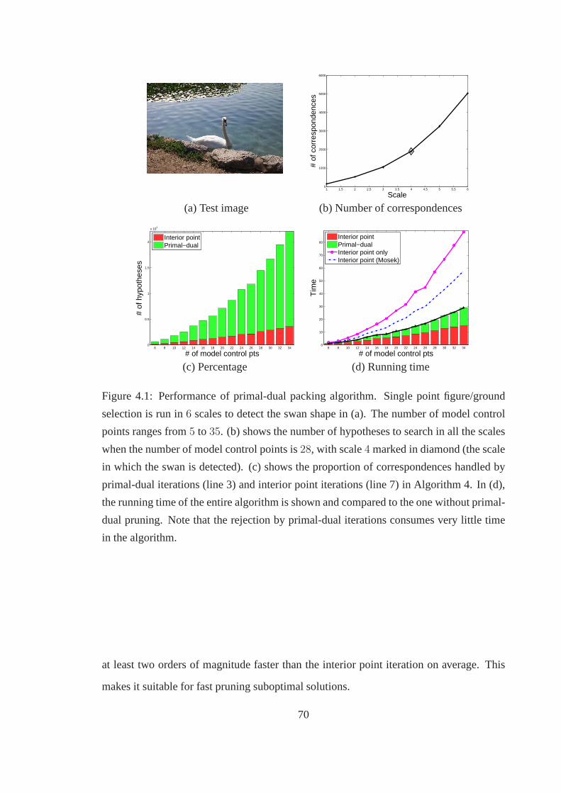
1 1.5 2 2.5 3 3.5 4 4.5 5 5.5 60

1000

2000

3000

4000

5000

6000

Scale

# of

cor

resp

onde

nces

(a) Test image (b) Number of correspondences

6 8 10 12 14 16 18 20 22 24 26 28 30 32 340

0.5

1

1.5

2

x 104

# of model control pts

# of

hyp

othe

ses

Interior pointPrimal−dual

6 8 10 12 14 16 18 20 22 24 26 28 30 32 340

10

20

30

40

50

60

70

80

# of model control pts

Tim

e

Interior pointPrimal−dualInterior point onlyInterior point (Mosek)

(c) Percentage (d) Running time

Figure 4.1: Performance of primal-dual packing algorithm.Single point figure/ground

selection is run in6 scales to detect the swan shape in (a). The number of model control

points ranges from5 to 35. (b) shows the number of hypotheses to search in all the scales

when the number of model control points is28, with scale4 marked in diamond (the scale

in which the swan is detected). (c) shows the proportion of correspondences handled by

primal-dual iterations (line 3) and interior point iterations (line 7) in Algorithm 4. In (d),

the running time of the entire algorithm is shown and compared to the one without primal-

dual pruning. Note that the rejection by primal-dual iterations consumes very little time

in the algorithm.

at least two orders of magnitude faster than the interior point iteration on average. This

makes it suitable for fast pruning suboptimal solutions.

70

4.5 Summary

We have shown that the LPs arising from contour packing do notneed to be solved ex-

actly for most of the time. The contour packing LP is first reduced to a fractional cover-

ing problem. We borrow the idea of primal-dual combinatorial algorithms that are able

to prune and bound packing and covering problems through duality and efficient ora-

cles. We develop an algorithm applying these ideas to singlepoint figure/ground selection

which involves massive LP instances. Most of these LPs can beefficiently pruned by the

primal-dual combinatorial algorithm, without resorting to solve the original LPs explic-

itly. Preliminary results confirm that the primal-dual algorithms can greatly relieve the

computational burden from standard LP solvers. We plan to explore more applications of

the algorithm in set-to-set matching.

71

Chapter 5

Contour Packing with Model Selection

So far we have developed a framework that detects a subset of image contours matched

to a model shape in a holistic manner. Shape models involved in the previous chapter are

simply exemplars composed of a few contours. Although the set-to-set matching method

endows the model the ability to accommodate different contour fragmentations, a fixed

target shape cannot handle large object deformations in images. Deformations often gen-

erate a combinatorial configuration space with exponentially many poses. This makes

brute-force search for the best exemplar prohibitive in practice. Moreover, it deepens

the discrepancy between the model and image shape descriptions because both side have

exponentially many configurations now.

In this chapter we push contour packing further to relate bottom-up contours to top-

down deformable parts beyond exemplars, addressing a bigger representation gap. We

study the challenging problem of articulated human pose estimation from unsegmented

images. A compact model representation is developed to encode exponentially many poses

via a few configuration selection variables on a tree. The set-to-set matching method ex-

tended for this new model representation can search and compare holistic shape features

of both image contours and model parts on the fly. This alleviates the reliance on local

shape features of parts, which often causes many false detections in clutter. The parallel

search over holistic shape features can be efficiently approximated by an LP-based com-

putational solution. We demonstrate results of human pose estimation on baseball player

72

images with wild pose variations.

5.1 Overview

Estimating poses for deformable or articulated objects is achallenging problem for two

reasons. The first reason is the large number of degrees of freedom to be estimated. Due

to the extreme pose variations, prior knowledge is of limited use in guiding the search.

Second, images are often cluttered and bottom-up detectionof parts is usually prone to

error. Again this is due to the fact that shape is a global percept – a part is seldom salient

without the whole shape.

For articulated objects, contour is a compact and effectiveshape representation. How-

ever, finding the foreground contours and estimating the object poses or articulations is a

circular problem. One individual bottom-up contour can hardly cover the entire object by

itself. If we know the right set of contours composing the foreground object, then we can

recognize the object by matching against a set of candidate models or exemplars. On the

other hand, this becomes circular because grouping contours into an object shape requires

the correct model. We can think of this problem as a puzzle of two parallel searches, one

for finding the right foreground contour grouping and one forgenerating the correct object

model. A naive approach to this would result in an exponential search.

We propose an active search method that finds the correct object contour grouping and

model configuration in one step. To encode this search, we extend the selection variables

which can be turned ON and OFF in Chapter 3. On the image side, each contour acts as

an integral unit that can either be selected or discarded as awhole. On the model side,

we deform a decomposable articulated model. Recognition isachieved if the model pose

matches the image foreground. We have developed a method forgenerating a holistic

shape descriptor based on these ON/OFF selection variables. Computationally this leads

to solving an integer program and a subsequent linear programming relaxation. A discrete

solution can be recovered using dynamic programming (DP) todiscretize the continuous

solution of linear programming relaxation.

73

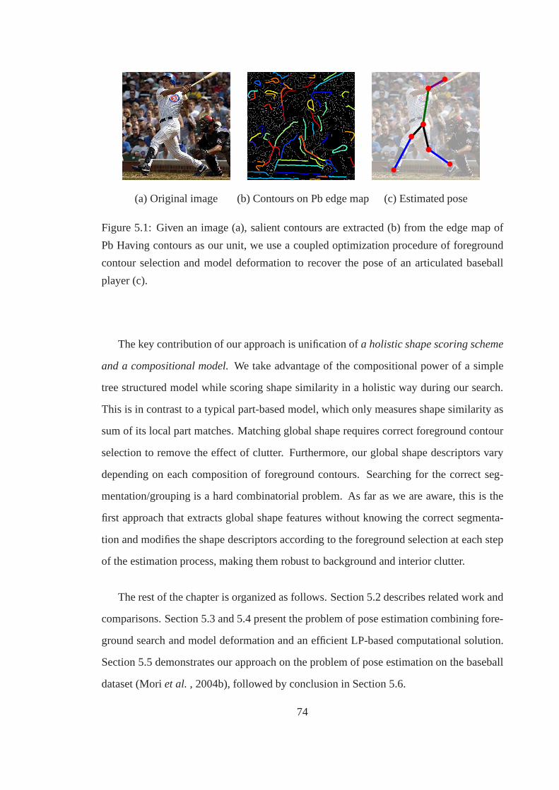
(a) Original image (b) Contours on Pb edge map (c) Estimated pose

Figure 5.1: Given an image (a), salient contours are extracted (b) from the edge map of

Pb Having contours as our unit, we use a coupled optimizationprocedure of foreground

contour selection and model deformation to recover the poseof an articulated baseball

player (c).

The key contribution of our approach is unification ofa holistic shape scoring scheme

and a compositional model.We take advantage of the compositional power of a simple

tree structured model while scoring shape similarity in a holistic way during our search.

This is in contrast to a typical part-based model, which onlymeasures shape similarity as

sum of its local part matches. Matching global shape requires correct foreground contour

selection to remove the effect of clutter. Furthermore, ourglobal shape descriptors vary

depending on each composition of foreground contours. Searching for the correct seg-

mentation/grouping is a hard combinatorial problem. As faras we are aware, this is the

first approach that extracts global shape features without knowing the correct segmenta-

tion and modifies the shape descriptors according to the foreground selection at each step

of the estimation process, making them robust to backgroundand interior clutter.

The rest of the chapter is organized as follows. Section 5.2 describes related work and

comparisons. Section 5.3 and 5.4 present the problem of poseestimation combining fore-

ground search and model deformation and an efficient LP-based computational solution.

Section 5.5 demonstrates our approach on the problem of poseestimation on the baseball

dataset (Moriet al. , 2004b), followed by conclusion in Section 5.6.

74

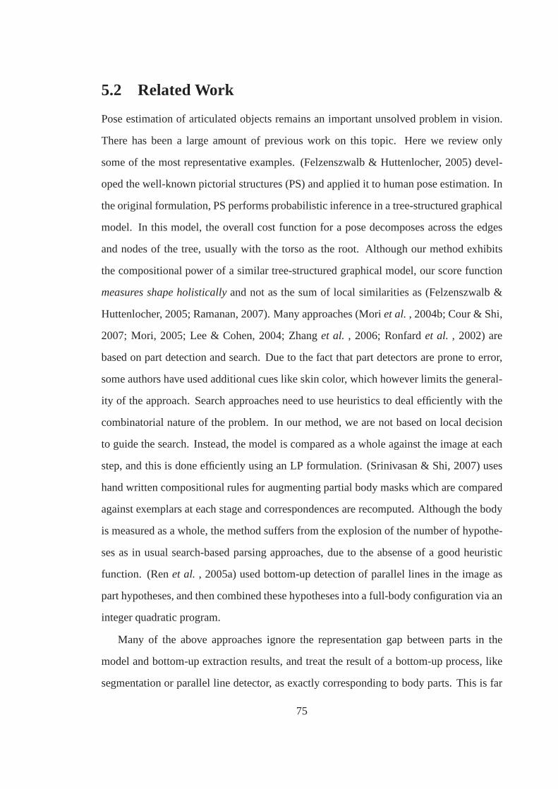
5.2 Related Work

Pose estimation of articulated objects remains an important unsolved problem in vision.

There has been a large amount of previous work on this topic. Here we review only

some of the most representative examples. (Felzenszwalb & Huttenlocher, 2005) devel-

oped the well-known pictorial structures (PS) and applied it to human pose estimation. In

the original formulation, PS performs probabilistic inference in a tree-structured graphical

model. In this model, the overall cost function for a pose decomposes across the edges

and nodes of the tree, usually with the torso as the root. Although our method exhibits

the compositional power of a similar tree-structured graphical model, our score function

measures shape holisticallyand not as the sum of local similarities as (Felzenszwalb &

Huttenlocher, 2005; Ramanan, 2007). Many approaches (Moriet al. , 2004b; Cour & Shi,

2007; Mori, 2005; Lee & Cohen, 2004; Zhanget al. , 2006; Ronfardet al. , 2002) are

based on part detection and search. Due to the fact that part detectors are prone to error,

some authors have used additional cues like skin color, which however limits the general-

ity of the approach. Search approaches need to use heuristics to deal efficiently with the

combinatorial nature of the problem. In our method, we are not based on local decision

to guide the search. Instead, the model is compared as a wholeagainst the image at each

step, and this is done efficiently using an LP formulation. (Srinivasan & Shi, 2007) uses

hand written compositional rules for augmenting partial body masks which are compared

against exemplars at each stage and correspondences are recomputed. Although the body

is measured as a whole, the method suffers from the explosionof the number of hypothe-

ses as in usual search-based parsing approaches, due to the absense of a good heuristic

function. (Renet al. , 2005a) used bottom-up detection of parallel lines in the image as

part hypotheses, and then combined these hypotheses into a full-body configuration via an

integer quadratic program.

Many of the above approaches ignore the representation gap between parts in the

model and bottom-up extraction results, and treat the result of a bottom-up process, like

segmentation or parallel line detector, as exactly corresponding to body parts. This is far

75

01

0

11

0

0

1

00 20

2

head

1 0 0

torso

1’

0 10

01 0

upper leg

2’

contour selection indicators

Image Contour Selection Model Configuration SelectionHolistic Matching

joint point selection indicators

Figure 5.2: Holistic shape matching. Our search has two parallel process, each encoded

by a selection variable. On the image side (left), contour selection variables turn image

contours ON and OFF assigning them to foreground or background respectively. This

results in all feasible shapes on the image side. On the modelside, selection variables

assign configurations to each model part in the tree structure. The two shapes, one derived

from the image and one from the model, are compared to each other using a holistic shape

feature. When the two match, recognition and pose estimation are achieved. Therefore

the recognition task amounts to finding the optimal selection on both the image and the

model side.

from being true in many cases. For example, in a straight leg you cannot expect to obtain

the upper and lower part of the leg separately. Our holistic view of shape surpasses this

difficulty,

5.3 Holistic Shape Matching

In this section, we first present the pose estimation formulation in terms of image contours

and model parts. Then we introduce our articulated model representation, with an active

shape description built in. The design of the active model shape descriptor is the key to

holistic shape matching.

5.3.1 Formulation of Pose Estimation Problem

Starting with contours as our basic units in the image, we develop the following formula-

tion.

76

Pose Estimation Problem.Given imageI represented by a set of contours and modelMrepresented by a set of parts:

• Image:I = {CI1 , C

I2 , . . . C

I|I|}, CI

k is thekth contour;

• Model:M = {PΘ1 , PΘ

2 , . . . PΘ|M|} wherePΘ

k is thekth part of the model andΘ is a

family of global parameters controlling model deformation.

We would like to select the best subsetIsel ⊆ I andΘ such that the shapes composed

by Isel and model partsPΘk are most similar as scored by global shape descriptors (see

Fig. 5.2). Note that this is anotherset-to-setmatching since there might not exist a one-

to-one mapping between selected image contours and contours of model configurations,

even though they have similar overall shapes. For example, elongated contours might

span multiple parts. We introduce the contour selection indicatorxsel ∈ {0, 1}|I|×1 over

all contours in theentiretest image defined as

(IMAGE CONTOUR SELECTION) xselℓ =

1 Contour CI

ℓ is selected

0 otherwise(5.1)

Accordingly we introduce a set of configuration selection indicatorsypart = {ykΘ} over all

partsPΘk in the model as

(MODEL CONFIGURATION SELECTION) ykα =

1 Part Pk selects config. α ∈ Θ

0 otherwise

(5.2)

Notice that since there is an infinite number of poses defined by Θ, resulting in an infinite

number of choices for our selection variables. We will show later that the selectionykα on

model articulation can be decomposed and simplified to limited choices by borrowing the

compositional power of a tree structure model. This problemstatement is similar to the

one in Section 3.2. Parts with different configurations (ypart) replace contours (ysel) as

tokens in model representation to handle articulation. Theshapes generated from the two

77

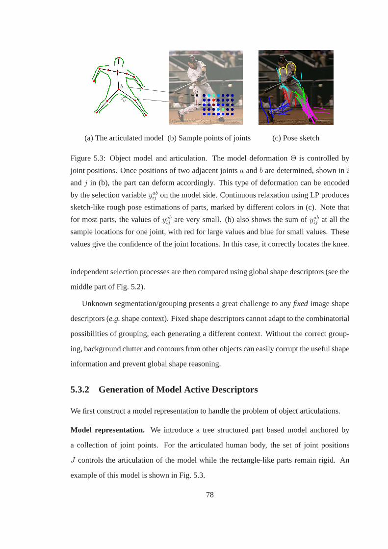
b

azabij

i

j

(a) The articulated model (b) Sample points of joints (c) Pose sketch

Figure 5.3: Object model and articulation. The model deformation Θ is controlled by

joint positions. Once positions of two adjacent jointsa andb are determined, shown ini

andj in (b), the part can deform accordingly. This type of deformation can be encoded

by the selection variableyabij on the model side. Continuous relaxation using LP produces

sketch-like rough pose estimations of parts, marked by different colors in (c). Note that

for most parts, the values ofyabij are very small. (b) also shows the sum ofyab

ij at all the

sample locations for one joint, with red for large values andblue for small values. These

values give the confidence of the joint locations. In this case, it correctly locates the knee.

independent selection processes are then compared using global shape descriptors (see the

middle part of Fig. 5.2).

Unknown segmentation/grouping presents a great challengeto anyfixed image shape

descriptors (e.g.shape context). Fixed shape descriptors cannot adapt to thecombinatorial

possibilities of grouping, each generating a different context. Without the correct group-

ing, background clutter and contours from other objects caneasily corrupt the useful shape

information and prevent global shape reasoning.

5.3.2 Generation of Model Active Descriptors

We first construct a model representation to handle the problem of object articulations.

Model representation. We introduce a tree structured part based model anchored by

a collection of joint points. For the articulated human body, the set of joint positions

J controls the articulation of the model while the rectangle-like parts remain rigid. An

example of this model is shown in Fig. 5.3.

78

Each model part includes two joint pointsa, b and a set of contours whose relative

positions to these joints are fixed. Therefore each model part appears to be a rigid shape

template, described byPab = {Ck(a, b)} whereCk(a, b)’s are contours as a function of

a, b. The image positionsi(a), j(b) of the two joint points uniquely determine a rigid

transformation (translation, rotation, and scaling) of the model part. In practice, we found

it sufficient to describe object deformation, though more joint points could be added in

general.

The collection of joint pointsa, b, c, ... of all model parts uniquely defines a legal pose

if the resulting template isconnectedat joint points. For example, the lower joint point

of a thigh has to be hooked with the upper joint point of a leg (at the knee). The model

participates in the matching process as a set of contours that compose the parts, which are

a function of the compatible configuration of the joint points as shown in Fig. 5.3. We

need to clarify that it is not important in which way the contours are fragmented on the

model side, as long as all together it composes a legal configuration of joint points. Hence

the shape is measured as a whole and all the contours on the model side participate in the

matching process.

With the exact model representation, we refine our part configuration selection variable

ykα in eq. (5.2) to encode the selection of a model part configuration as follows:

yabij =

1 Jointa is mapped to image sample pointi andb mapped toj

0 otherwise(5.3)

The model can also be defined as a set of part configurationsM = {Pab(i, j) : a, b ∈J, i, j ∈ S} with J andS being the set of joint points and the set of sample points. The

sample points are the possible placement of the model joint points. The setS could be

as simple as rectangular grid locations. We would like to select a set of legal one-to-

one correspondences betweenJ andS, such that the shape of the model resulting from

these configurations is as close as possible to the shape composed by the selected image

contours.

Now we are ready to express the holistic shapes by these modelpart configurations.

79

Shape Contexts (SC) centered at sample points are chosen as our basic shape descriptors,

which is ideal for capturing the bending and rotation of bodyparts such as limbs. A model

contribution matrixV Mi at sample pointi is defined similar to the image contribution

matrixV Ii in eq. (3.4):

V Mi (k, l) = # of points in bink from partPl (5.4)

Recall that the image SC is written as follows in eq. (3.5):

scIi (k) = (V I

i · xsel)k (5.5)

It is straightforward to see that SC on modelscMi can be generated similar to eq. (3.5),

depending on exponentially many combinations of model partconfigurations:

scMi (k) = (V M

i · ypart)k (5.6)

We treatypart as a selection vector by concatenating all the joint point selection indicators

yabij in eq. (5.3).

5.4 Computational Solution for Matching Holistic Fea-

tures

Our goal is to findxsel and ypart such that they produce similar global shape context

features at the view points considered. For the model with tree structure defined above,

we present an efficient computational solution. The holistic matching of selected image

contours and model deformation amounts to minimize the difference betweenscIi and

scMi . This can be summarized by putting eq. (3.5) and eq. (5.6) together:

(CONTOUR PACKING LP WITH MODEL SELECTION)

minxsel,ypart

∑

i

Di(scIi , sc

Mi ) =

∑

i

‖V Ii · xsel − V M

i · ypart‖ (5.7)

s.t.∑

i

zabij =

∑

k

zbcjk, ∀j ∈ J (Connectivity between parts) (5.8)

∑

ij

zabij = 1, ∀a, b (Uniqueness of part assignment) (5.9)

80

The first constraint ensures the connectivity between the neighboring parts of the model.

The second constraint ensures that each model part is present. We can relax this constraint

to account for possibly occluding or missing parts, essentially introducing selection on the

model side. We omit this extension for simplicity.

Direct optimization of the integer programming eq. (5.9) isa hard combinatorial search

problem. Basically at each step of the search we need to update our shape descriptors ac-

cording to the current image contour selection and model deformation and compare them

using eq. (5.7). To deal with the combinatorial nature of theproblem we relax and solve

it using linear programming (LP). Essentially we exploit linear form of shape context

descriptors to formulate the holistic matching with contour and part selection. This tech-

nique enables us to generate the space of all the combinatorial features via precomputing

contribution matricesV I andV M .

Discretization via Dynamic Programming (DP).Holistic search using the above com-

putational solution produces sketch-style rough estimation of the poses and locations of

joints (see Fig. 5.3). Rounding the linear programming solution of ypart directly does not

guarantee the selected model parts to be connected. Therefore, we search for assignments

of joints to image locations with the largest sum of connectionsypart while maintaining the

model structure. We optimize∑

(a,b)∈J yabij whereyab

ij is the linear programming solution.

Since the model has a tree structure, the optimum can be foundby a simple DP.

Our treatment is different from performing pictorial structure directly in two aspects.

First, searching for the optimalypart has taken into account the global context beyond

pairwise part connections. In contrast, the pairwise cost contains much less information

and hence has limited discriminative power. Second we are able to utilize salient image

structures such as long contours and large regions despite the semantic gap between them

and the model parts. Hence we do not need to design part detector which itself could be a

much harder problem than recognizing the whole shape.

Bottom-up driven sampling of joint points. The holistic search of pose should not

start purely in a top-down sense, and bottom-up grouping should be exploited as much as

81

possible. Contours and regions are grouped into symmetric ribbons. Therefore, we detect

termination points on medial axis of these ribbons as candidates of the protrusion points

(e.g. foot). We start sampling all possible locations of other joint points w.r.t these points

under part rotation and stretching (see Fig. 5.3). These hypotheses suggest possible model

part deformations and they are further verified by the holistic search.

5.5 Experiments

Our approach is tested on a challenging dataset of baseball player images collected from

the web as well as the one used in (Moriet al. , 2004b). The dataset contains a wide

range of pose variations and severe background clutter (seeFig. 5.1 for an example). The

combination of these two factors makes pose estimation verychallenging.

We start with contour grouping described in Chapter 2. It produces 100 contours for

each image on average. Since arms are often missing in the bottom-up contour detection

due to occlusion and confusion with background, we use the model containing only head,

torso, and lower body with 7 joint points. For this experiment, we take rough bounding

boxes as inputs since our focus is pose estimation rather than hypothesis generation. We

sample candidates of joints in head, torso and upper leg fromgrid points in the image.

Additional sample joint points are extracted from termination point of medial axis. Each

joints have roughly 50 sample points, which will generate507×100 = 7.813 hypotheses if

brute force search was done. Our linear programming search is efficient: typically 20-30

seconds per images by itself.

We run our method using global shape context without image contour selection and

the results are much worse due to overwhelming background clutter. We also test our

method using a smaller shape context window without selection. The results are better

than the global one without selection but worse than large one with selection. This verifies

the importance of holistic matching. Active shape featureswe introduce are robust against

clutter and can accurately recover the correct poses. Our results outperform (Ramanan,

2007) which uses iterative PS, as shown in Fig. 5.4 (d), (e).

82

5.6 Summary and Future Work

We have presented a holistic shape matching technique with adeformable template for

pose estimation and segmentation of articulated objects. We introduce the concept of ac-

tive context features and present an efficient computational framework for their compar-

ison. We demonstrate results in the baseball dataset but ourapproach is general enough

for any other category of articulated objects. Future work includes the incorporation of

additional constraints on model deformation to further restrict the search space and the in-

troduction of part selection on the model side to deal with missing parts due to occlusion.

Future work also includes the incorporation of further bottom-up cues like segments to

help guide the model deformation.

83

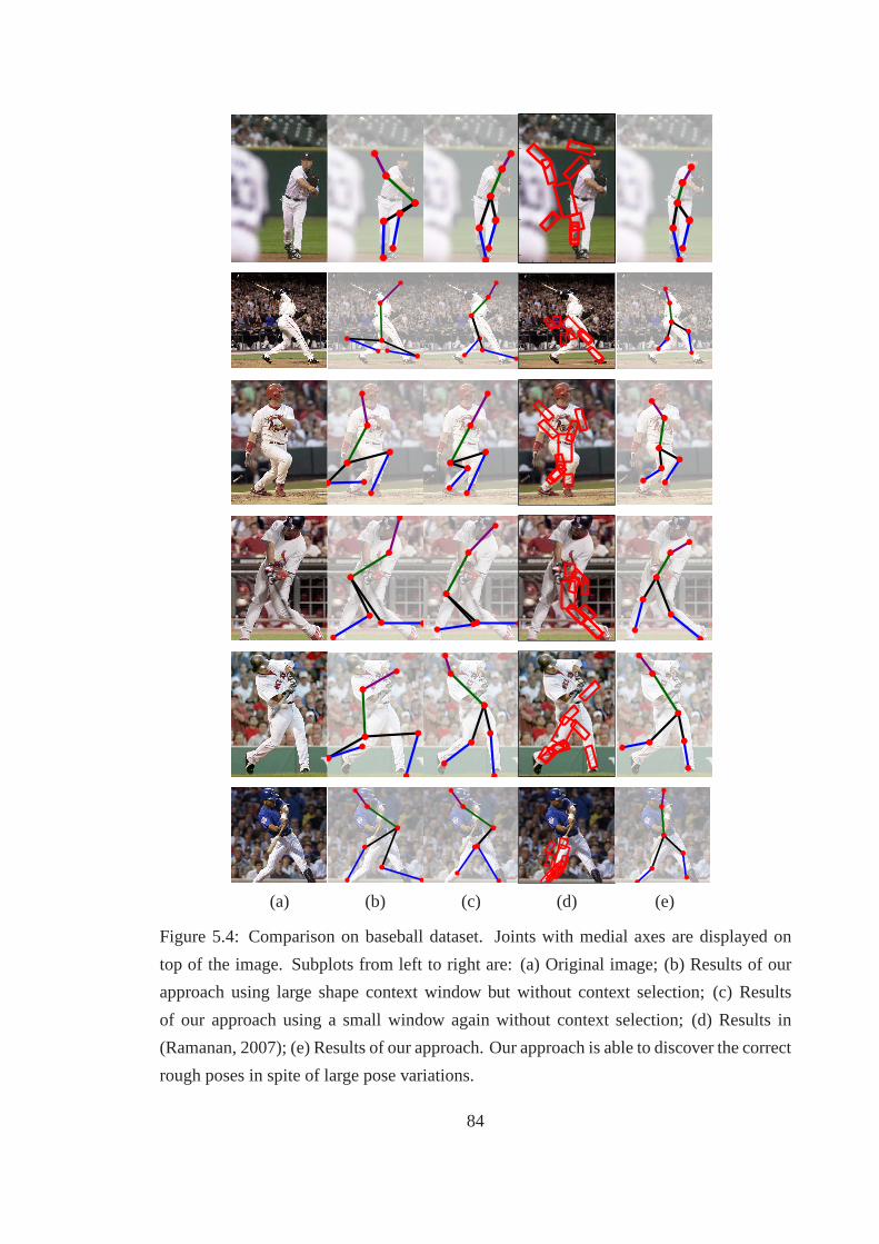
50

100

150

200

50

100

150

200

50

100

150

200

50

100

150

200

50

100

150

200

50

100

150

200

(a) (b) (c) (d) (e)

Figure 5.4: Comparison on baseball dataset. Joints with medial axes are displayed on

top of the image. Subplots from left to right are: (a) Original image; (b) Results of our

approach using large shape context window but without context selection; (c) Results

of our approach using a small window again without context selection; (d) Results in

(Ramanan, 2007); (e) Results of our approach. Our approach is able to discover the correct

rough poses in spite of large pose variations.

84

50

100

150

200

50

100

150

200

50

100

150

200

50

100

150

200

50

100

150

200

50

100

150

200

(a) (b) (c) (d) (e)

Figure 5.5: More results on baseball dataset. Joints with medial axes are displayed on

top of the image. Subplots from left to right are: (a) Original image; (b) Results of our

approach using large shape context window but without context selection; (c) Results

of our approach using a small window again without context selection; (d) Results in

(Ramanan, 2007); (e) Results of our approach. Our approach is able to discover the correct

rough poses in spite of large pose variations.

85

Chapter 6

Region Packing

Salient objects tend to pop out as contiguousregions– a group of pixels that delineate

themselves from the rest of the image. As a complement to contours, regions play an

important role in object detection. First of all, regions convey global shape information

which is not available from local image features. Boundaries of regions often contain half

complete object silhouettes whose shapes are clearly recognizable. Secondly, unlike con-

tours that could be open ended, regions are closed and therefore specify the figure/ground

labeling of the image. The figure/ground segmentation ensures the right spatial support

of objects, and blocks irrelevant features from clutter. Thirdly, segmenting the image into

regions helps to arouse visual attention to certain objects. Exhaustive search such as scan-

ning the entire image could be avoided by reasoning salient regions and their surroundings.

In this chapter, we develop a packing framework that detectsholistic shapes from

bottom-up regions, extending contour packing in the previous chapters. Starting from

region segments with bags of shape features, we try to pack image and model features

into histograms. A subset of regions are matched to the modelif they can pack the same

set of features as the model. Due to the different topology ofregions, the underlying

combinatorial problem is relaxed to Semi-Definite Programs(SDP) instead of LPs. This

formulation not only tackles the problem of region fragmentations, but is also able to

incorporate bottom-up grouping saliency into a unified framework.

86

6.1 Overview

The importance of regions to object recognition has long been noticed by many researchers

(Basri & Jacobs, 1997). Regions along with their boundariesare used extensively to build

shape descriptions in medial axis (Blum, 1967), and its successors such as shock graphs

(Siddiqiet al., 1999), conformal mapping (Sharon & Mumford, 2006), and Poisson equa-

tion based descriptors (Gorelicket al. , 2006). Regions provide a global account for ob-

ject shapes since they are large enough to capture the long-range geometric dependency.

They are also shown to be useful for searching and parsing semantical parts (Srinivasan &

Shi, 2007), as well as handling object deformation (Ling & Jacobs, 2005). However, all

these methods assume that the segmentation of the entire object can be obtaineda priori,

which is rarely the case in detection. The global region-based descriptors change drasti-

cally when fragmentations and leakages occur in real images. It is not clear how a shape

descriptor can guide the search over exponentially many different segmentations for the

desired shape.

Many works based on Bag-of-Features (BoF) exploit regions from bottom-up seg-

mentation as the spatial support of local features (Liet al. , 2009; Gupta & Davis, 2008;

Galleguilloset al. , 2008; Malisiewicz & Efros, 2008). However, geometry as well as

object part information is completely missing in BoF. Spatial histogram on local features,

e.g.HOG (Dalal & Triggs, 2005) has put geometry back to the representation. However,

the extraction of these local features is independent of their underlying spatial support.

Selecting the right features associated with the foreground relies on discriminative classi-

fiers, which usually requires a large number of training examples. The fixed, rectangular

spatial histogram also poses the problem of object alignment. Regions have been used in

verifying hypotheses from top-down classifiers in (Wanget al. , 2007; Ramanan, 2007),

showing the potential of reasoning the spatial support of detection.

Inspired by all the previous approaches, we proposeregion packing, a shape matching

method that reasons the holistic shape composed by a set of region segments, and provides

87

an efficient search over their combinations. Region packingbears the same spirit as ear-

lier works that the overall rather than the individual shapeof region boundaries should be

measured. It incorporates a different shape description than medial axis,etc, using spatial

histograms with a large spatial extent developed in Chapter3. This representation enables

exploiting the composition and closure of regions, such that combinatorially many seg-

mentations can be encoded compactly, and an efficient searchcan be performed without

enumerating all the hypotheses.

The main technical challenge is the unpredictable fragmentations of region segments.

Boundaries between two segments can be either real or fake depending on which segment

is foreground. Removing these fake boundaries (and hence merging the regions) is com-

plicated by different fragmentations of images. To overcome this challenge, two recent

works (Guet al. , 2009) and (Todorovic & Ahuja, 2008) are most related to our approach.

In (Guet al. , 2009), discriminative shape features are learned from some “typical” object

segments, and combined in a BoF way. In (Todorovic & Ahuja, 2008), subgraphs in the

segmentation hierarchy are explicitly compared during shape matching, which amounts to

memorizing all possible different fragmentations. However, structures of these subgraphs

might not be repeatable with limited training images. Region packing adjusts shape fea-

tures according to the set of regions that are merged to form the foreground, and therefore

unaffected by fragmentations. Unlike (Guet al. , 2009), we do not assume that individ-

ual region segments are simultaneously distinctive and repeatable. We also noticed that

regions are not fragmented randomly, hence they should not be merged blindly. The pref-

erences from various bottom-up grouping cues can naturallyfit into the framework.

The rest of this chapter is organized as follows. We start with the basic holistic re-

gion matching in Section 6.2. This problem is formulated as abipartite graph packing

due to the topology of region. Then we develop an SDP-based approximation which can

compactly express bipartite graph packing. In Section 6.3,we show that various grouping

cues such as figure/ground, boundary saliency and junction configurations can be read-

ily incorporated into the framework. The proposed approachis tested on the challenging

88

ETHZ Shape Classes in Section 6.4, producing comparable results to the state-of-the-art

region-based methods.

6.2 Holistic Region Matching

The main problem to solve is to match object shapes composed by regions in a holistic

way, without knowing which regions belong to foreground. Westart by formalizing this

problem as follows.

Definition of holistic region matching. Given an imageI and a modelM decomposed

into two sets of disjoint regions:

• Image:I = RI1 ∪ RI

2 ∪ . . . ∪ RI|I|, with RI

k being thekth region andRIi ∩ RI

j = ∅

for any two regionsi 6= j;

• Model:M = RM1 ∪RM

2 ∪. . .∪RM|M|, with RM

l being thelth region andRMi ∩RM

j = ∅

for any two regionsi 6= j,

we would like to find region subsetsIsel ⊆ {RIi } andMsel ⊆ {RM

i }, such that their

boundary shapesB(Isel) andB(Msel) match. Each regionRIk andRM

l contains a con-

nected set of pixels. The operatorB(·) is defined as the boundary generated by the mask

of a region set. This can be written formally as:

B(R) = {x : N(x) ∩⋃

Ri∈R

Ri 6= ∅, N(x) ∩ I \ (⋃

Ri∈R

Ri) 6= ∅} (6.1)

Herex is a pixel andN(x) represents the set of its neighboring pixels (3×3 neighborhood).

Since bottom-up region segmentation could also have unpredictable fragmentations that

are different from the model (see Fig. 6.1), we adapt the set-to-set matching paradigm

developed in Chapter 3 to overcome this representation problem in the following sections.

Before diving into the solutions to the problem, we would like to highlight two key

conceptual differences between region packing and contourpacking. First, using regions

as the basic units in packing exploitsclosure, a stronger constraint than its contour peer:

the object boundaries have to be closed. In contrast, a set ofopen contours could be

89

…

…

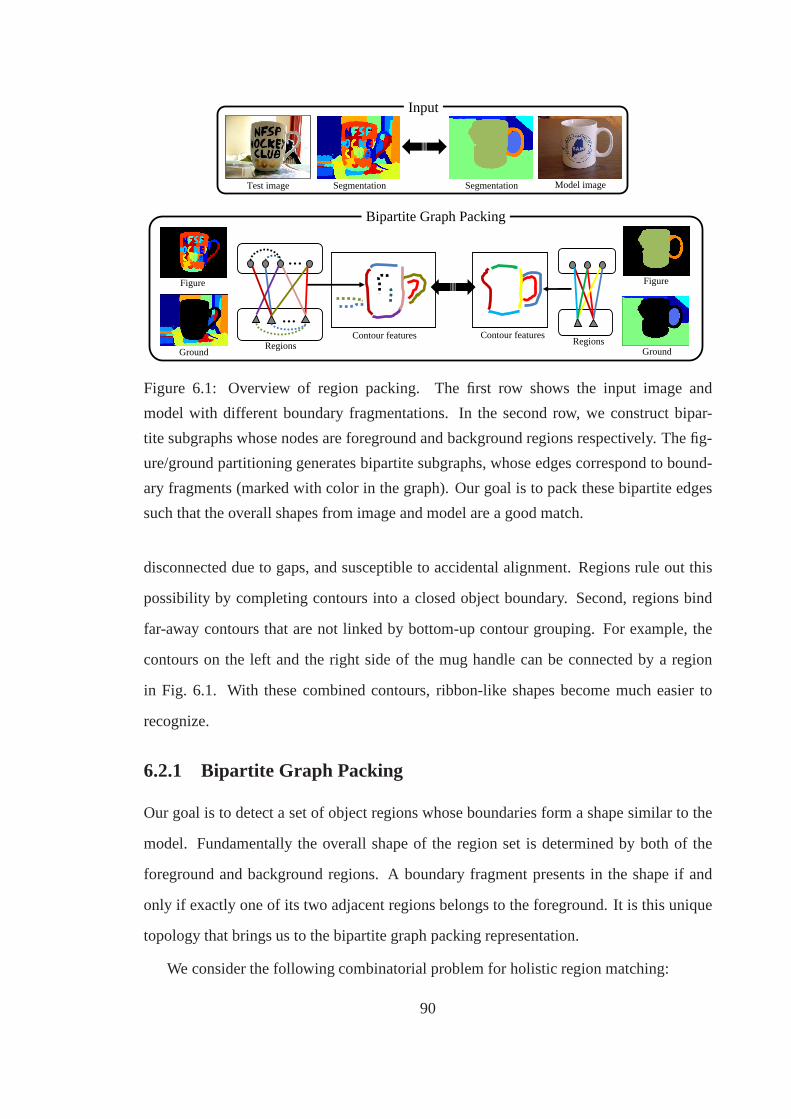
Test image Segmentation Model imageSegmentation

Input

Figure

Ground

Figure

Ground

Bipartite Graph Packing

Contour featuresContour featuresRegionsRegions

Figure 6.1: Overview of region packing. The first row shows the input image and

model with different boundary fragmentations. In the second row, we construct bipar-

tite subgraphs whose nodes are foreground and background regions respectively. The fig-

ure/ground partitioning generates bipartite subgraphs, whose edges correspond to bound-

ary fragments (marked with color in the graph). Our goal is topack these bipartite edges

such that the overall shapes from image and model are a good match.

disconnected due to gaps, and susceptible to accidental alignment. Regions rule out this

possibility by completing contours into a closed object boundary. Second, regions bind

far-away contours that are not linked by bottom-up contour grouping. For example, the

contours on the left and the right side of the mug handle can beconnected by a region

in Fig. 6.1. With these combined contours, ribbon-like shapes become much easier to

recognize.

6.2.1 Bipartite Graph Packing

Our goal is to detect a set of object regions whose boundariesform a shape similar to the

model. Fundamentally the overall shape of the region set is determined by both of the

foreground and background regions. A boundary fragment presents in the shape if and

only if exactly one of its two adjacent regions belongs to theforeground. It is this unique

topology that brings us to the bipartite graph packing representation.

We consider the following combinatorial problem for holistic region matching:

90

Definition. Given a graphG = (V, E) where

• Graph nodesV = {R1, R2, ..., Rn} represent image regions.

• Graph edgesE = {Bij : Bij = B(Ri)∩B(Rj)} correspond to boundary fragments

shared by adjacent regions.

Given any partition of regionsV = F ∪ F with F as foreground andF as background,

we evaluate a shape cost functionCp(F, F ) to measure the shape similarity of boundaries

formed byF andF compared to the object model. For holistic shape matching, we pose

the question: can we find an optimal bipartite subgraphGsub(F, F ) minimizing shape cost

Cp(F, F )? We refer to this general problem asbipartite graph packingsince the cost

Cp(F, F ) is determined over a biparitite subgraph.

An appropriate shape cost functionCp(F, F ) plays an important role conceptually and

computationally. If there exists one-to-one correspondences between image and model

boundaries, one can defineC(F, F ) as a linear combination of costsWij on the edgesEij .

Minimizing a linear cost results in standard graph-cut problems (MinCut or MaxCut).

Because of the unpredictable fragmentations of image region boundaries (see Fig. 6.1),

set-to-set matching on region boundaries arises. A simple linear cost on bipartite graph is

insufficient to match the holistic shapes of two set of boundaries. We adopt the Context

Selective Shape Features in Chapter 3 as:

Cp(F, F ) = ‖V I · x− scM‖1, x ∈ {0, 1}|E| (6.2)

with xk = 1 if and only if edgeEk is a bipartite edge,i.e.Ek ∈ E(F, F ).

The bipartite graph packing with cost eq. (6.2) can be reduced to cardinality con-

strained and multicriteria cut problems (Bruglieriet al. , 2004; Bentzet al. , 2009), as

stated by the following theorem:

Theorem 6.1. The bipartite region graph packing problem consists in finding an optimal

bipartite subgraphGsub(F, F ) of the region graphG, which minimizes costCp(F, F ) de-

fined in eq. (6.2). It can be reduced to a cardinality constrained and multicriteria cut prob-

lem on a graphG′ associated withR positive edge weight functionsw(1),...,w(R) according

91

toR criteria. The cardinality constrained and multicriteria cut problem seeks a cutC with

cardinality at leastd:∑

Eij∈C 1 ≥ d, and allR criteria are satisfied:∑

Eij∈C w(k)ij ≤ b(k)

for k = 1, 2, ..., R.

Proof. Please see Appendix for details of the reduction.

The cardinality constrained and multicriteria multicut problems are in general NP-

hard1, as shown in (Bentzet al. , 2009). Therefore, finding a computationally feasible

approximation is the key to solve the original problem.

6.2.2 Approximation via Semidefinite Program (SDP)

We seek a relaxation to the above bipartite graph packing formulation via Semidefinite

Program (SDP), which has provided polynomial time approximations to many NP-hard

problems such as MaxCut (Goemans & Williamson, 1995). In thefollowing sections, we

will also demonstrate various constraints such as junctionconfigurations can be conve-

niently encoded in the SDP formulation.

First we define the region selection indicatorr ∈ Rn as:

(REGION SELECTION INDICATOR) ri =

+1, if regionRi ∈ foreground

−1, otherwise.(6.3)

Note that the definition ofr is different from the0/1 contour selection indicator in Chap-

ter 3 for simplicity in the subsequent formulation.

Next we introduce a graph indicator matrixZ ∈ Rn×n to be the Gram matrix of the

region selection indicatorr:

(GRAPH INDICATOR) Z = rrT (6.4)

Each entryZij is also a+1/ −1 indicator, with the diagonal to be ones:Zii = 1. The

graph indicatorZ fully characterizes a bipartite subgraph with nodesF = {i : ri = 1},F = {i : ri = −1}, and bipartite edgesE(F, F ) = {(i, j) : Zij = −1}. Moreover,Z is a

1However, MinCut which represents a single criteria cutwithoutany cardinality contraints, can be solvedin polynomial time.

92

positive semidefinite matrixZ � 0 because for any vectoru, we haveuTZu = uTrrTu =

(rTu)2 ≥ 0. a counterpart of the contour selector, we use a0/1 selection indicatorxsel

to specify figure/ground labels on boundary fragments that are shared by two adjacent

regions. These boundary fragments serve as the basic building blocks of the object shapes

just as contours in Chapter 3. Boundary fragments behave differently than contours in that

they can only be packed if exactly one of its two adjacent regions appears as foreground,

i.e.

xselk = 1⇔ (ri = 1 ∧ rj = −1) ∨ (ri = −1 ∧ rj = 1) (6.5)

This constraint can be rephrased in terms ofZ: (1− Zij)/2 = xselk sinceZij = rirj .

The overall shape composed by selected regions needs to be holistically matched to

the model shape. We adopt the contour packing cost eq. (3.7) as the packing function

Cp(F, F ) on bipartite edges, measuring the shape dissimilarity of a set of boundary frag-

ments generated by the selected regions (F ). For each control point correspondence, the

shape dissimilarity‖V I ·xsel− scM‖1 depends on which boundary fragments are selected

by xsel, with the contribution matrix of boundary fragmentsV I precomputed. We sum-

marize all the above components into the following SDP:

(REGION SELECTION SDP)

maxZ, xsel

‖V I · xsel − scM‖1 (6.6)

s.t.1− Zij

2= xsel

k , ∀Ri, Rj separated by fragmentk (6.7)

diag(Z) = 1 (6.8)

Z � 0 (6.9)

If the rank of matrixZ is 1, the optimal SDP solution is exactly the optimum of bipartite

graph packing. The non-convex constraintrank(Z) = 1 is dropped to obtain an SDP

problem, which is solvable by off-the-shelf SDP packages. After solving the optimal

graph matrixZ∗, we recoverr by computing its largest eigenvector. A binary selection on

regions can be obtained by thresholding the continuous eigenvector.

93

xselk+

rirj

xselk+

rirjrj

xselk−

ri

(a) Object boundary (b) True boundary 1 (c) True boundary 2 (d) False boundary

Figure 6.2: Figure/ground labeling on boundaries. The boundary of a swan along with

its foreground region is shown in (a). In the circled area, different figure/ground configu-

rations exist and need to be distinguished. Two true boundaries with opposite directions

in (b) and (c) appear due to the parallelism. (d) shows a falseboundary with incorrect

figure/ground labeling.

For the convenience of further discussion, we introduce a vectorization operatorsvec :

Sn 7→ Rn(n+1)/2 on the symmetric matrixZ ∈ Sn as:

svec(Z) = [Z11,√

2Z12, Z22, ...,√

2Z(n−1)n, Znn]T (6.10)

An important property of the operatorsvec is that it translates matrix inner product into

vector inner product:tr(Y Z) = svec(Y )Tsvec(Z). This allows us to define a transfor-

mation matrixT ∈ Rm×n(n+1)

2 to represent all the linear constraints in eq. (6.7) such that

T · svec(Z) = xsel. Note that sinceZii = 1, every entryxselk =

1−Zij

2in eq. (6.7) can be

written as a linear form insvec(Z). With the above notations, region selection eq. (6.6)

can be expressed more compactly as:

maxZ‖V I · T · svec(Z)− scM‖1 (6.11)

s.t. diag(Z) = 1, Z � 0

6.3 Representing Grouping Constraints

Expressing bipartite graph packing in a SDP form enables several important extensions to

bottom-up grouping constraints.

94

6.3.1 Figure/Ground

Up to this point we have not taken into account the figure/ground labeling of boundary

fragments. Selection of a boundary fragment does not specify which side of the fragment

belongs to the foreground object. In eq. (6.6), flipping the region indicator fromr to−r

produces the sameZ, and hence does not change the packing cost. This means foreground

and background are exchangeable for region packing. To remedy this problem, we add a

fictitious noder0 = 1 to represent the foreground. Any regions partitioned to thesame

side as the fictitious node will be labeled as foreground. This amendment adds one row

and one column toZ with Zi0 = ri. Accordingly, boundary fragments become directional:

the foreground region is always located on the right side of the boundary. The boundary

selection indicators are split into two copiesxselk = xsel

k+ + xselk− defined as follows:

xselk+ = (ri = 1) ∧ (rj = −1) =

ri + 1

2· 1− rj

2=

Zi0 − Zj0 − Zij + 1

4(6.12)

xselk− = (ri = −1) ∧ (rj = 1) =

1− ri

2· rj + 1

2=−Zi0 + Zj0 − Zij + 1

4(6.13)

Indicesi, j, k+, k− are organized in the following way. When traveling along thedi-

rection ofk+, the positive one ofri, rj (foreground region) lies on the right side of the

boundary; it lies on the left side when traveling alongk− (see Fig. 6.3).

The shape features also need changes to be compatible for thefigure/ground specifi-

cation. We split each edge orientation bin of shape context into two bins, encoding edges

pointing opposite directions. Now the contributions ofxselk+ andxsel

k− to the shape descrip-

tors are separated, and therefore a mismatch of figure/ground will be penalized.

6.3.2 Boundary Saliency

True objects not only match model well, but pop out from the background. Saliency of

segmentation can reduce many false positives by penalizingrandomly packed segments,

and favoring segments that can be easily cut out of the background (see Fig. 6.3.2). There-

fore, we introduce region grouping edgesEg, whose weights encode how well the regions

95

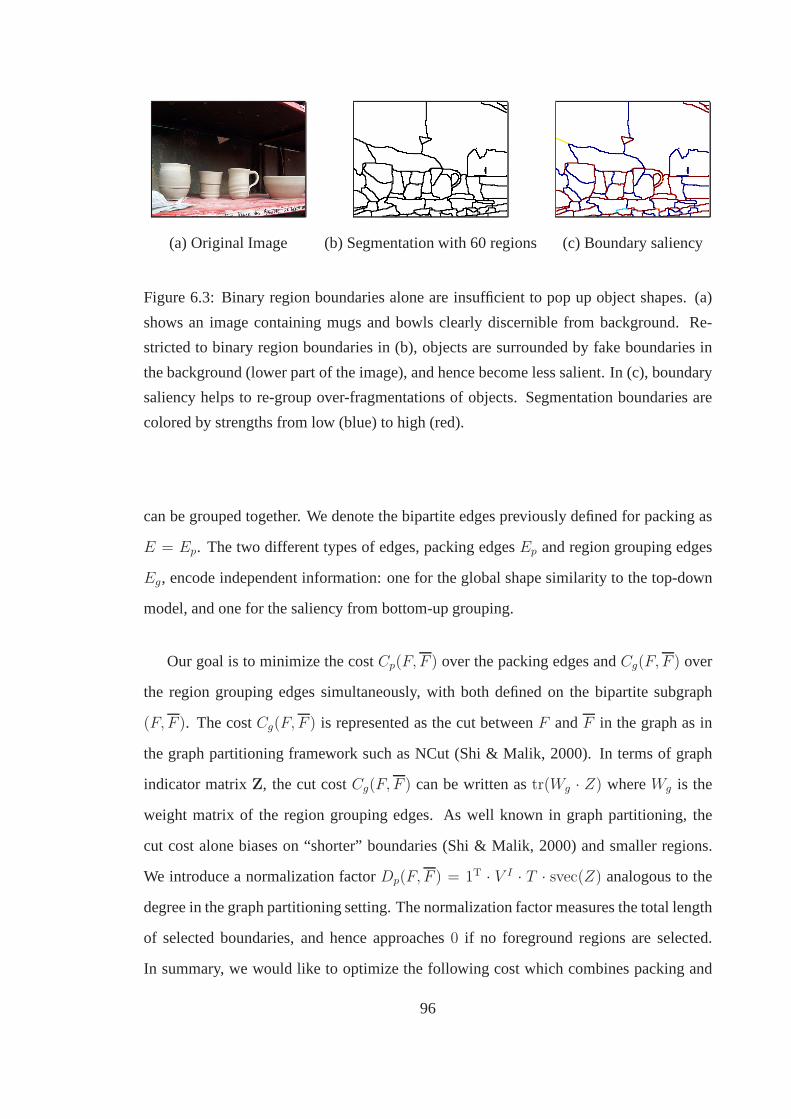
(a) Original Image (b) Segmentation with 60 regions (c) Boundary saliency

Figure 6.3: Binary region boundaries alone are insufficientto pop up object shapes. (a)

shows an image containing mugs and bowls clearly discernible from background. Re-

stricted to binary region boundaries in (b), objects are surrounded by fake boundaries in

the background (lower part of the image), and hence become less salient. In (c), boundary

saliency helps to re-group over-fragmentations of objects. Segmentation boundaries are

colored by strengths from low (blue) to high (red).

can be grouped together. We denote the bipartite edges previously defined for packing as

E = Ep. The two different types of edges, packing edgesEp and region grouping edges

Eg, encode independent information: one for the global shape similarity to the top-down

model, and one for the saliency from bottom-up grouping.

Our goal is to minimize the costCp(F, F ) over the packing edges andCg(F, F ) over

the region grouping edges simultaneously, with both definedon the bipartite subgraph

(F, F ). The costCg(F, F ) is represented as the cut betweenF andF in the graph as in

the graph partitioning framework such as NCut (Shi & Malik, 2000). In terms of graph

indicator matrixZ, the cut costCg(F, F ) can be written astr(Wg · Z) whereWg is the

weight matrix of the region grouping edges. As well known in graph partitioning, the

cut cost alone biases on “shorter” boundaries (Shi & Malik, 2000) and smaller regions.

We introduce a normalization factorDp(F, F ) = 1T · V I · T · svec(Z) analogous to the

degree in the graph partitioning setting. The normalization factor measures the total length

of selected boundaries, and hence approaches0 if no foreground regions are selected.

In summary, we would like to optimize the following cost which combines packing and

96

grouping:

Cp+g(F, F ) =Cp(F, F ) + Cg(F, F )

Dp(F, F )(6.14)

=‖V I · T · svec(Z)− scM‖1 + β · svec(Wg)

Tsvec(Z)

1T · V I · T · svec(Z)(6.15)

In spite of the normalization, the optimization problem eq.(6.15) can still be formu-

lated as SDP by introducing a normalized matrixY = Z/[1TV IT · svec(Z)]. Because

the normalization factor1TV IT · svec(Z) > 0, the matrixY is also positive semidefinite,

resulting in the following SDP:

maxY‖V I · T · svec(Y )− scM · Y11‖1 + β · svec(Wg)

Tsvec(Y ) (6.16)

s.t. 1TV IT · svec(Y ) = 1 (6.17)

diag(Y ) = Y11 (6.18)

Y � 0 (6.19)

Since we construct the graphs on the region segments rather than image pixels, group-

ing weightsWg directly include global grouping saliency. The weightWg(i, j) between

region segmentri andrj are computed by:

Wg(i, j) = exp(−d2

ij

2σ2)|Cut(ri, rj)| (6.20)

where |Cut(ri, rj)| is defined as the boundary length between the two segments. The

termdij is the geodesic distance in the eigenvector embedding spaceof NCuts between

cluster centers ofri andrj. The geodesic distance computes the shortest path distance

on weights defined as the point density in the embedding spaceformed by eigenvectors.

This measures how well the two regions can be separated. We would like to pointed

out the advantage of definingWg on the output of segmentation rather than original edge

magnitude, which makes the overall cost insensitive to image contrast changes. Moreover,

because entries inWg are normalized by the corresponding boundary lengths, the three

termsCP (F, F ), CG(F, F ), andDP (F, F ) in eq. (6.14) are balanced.

97

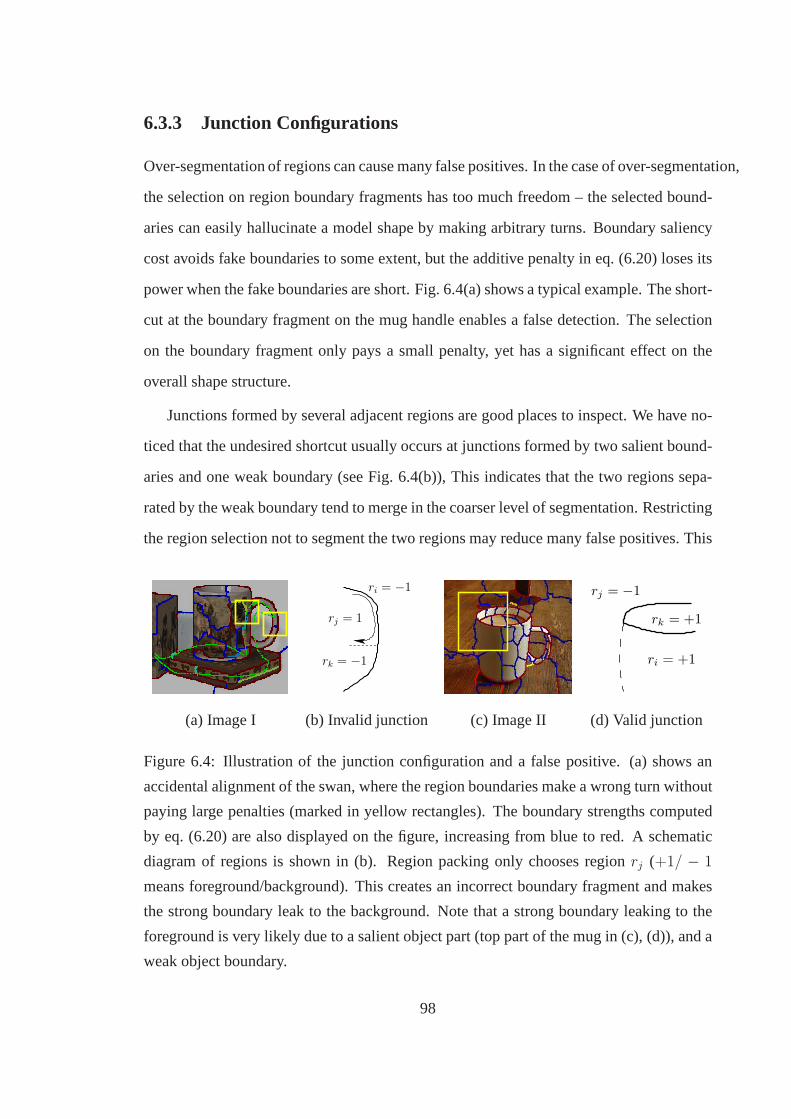
6.3.3 Junction Configurations

Over-segmentation of regions can cause many false positives. In the case of over-segmentation,

the selection on region boundary fragments has too much freedom – the selected bound-

aries can easily hallucinate a model shape by making arbitrary turns. Boundary saliency

cost avoids fake boundaries to some extent, but the additivepenalty in eq. (6.20) loses its

power when the fake boundaries are short. Fig. 6.4(a) shows atypical example. The short-

cut at the boundary fragment on the mug handle enables a falsedetection. The selection

on the boundary fragment only pays a small penalty, yet has a significant effect on the

overall shape structure.

Junctions formed by several adjacent regions are good places to inspect. We have no-

ticed that the undesired shortcut usually occurs at junctions formed by two salient bound-

aries and one weak boundary (see Fig. 6.4(b)), This indicates that the two regions sepa-

rated by the weak boundary tend to merge in the coarser level of segmentation. Restricting

the region selection not to segment the two regions may reduce many false positives. This

rk = −1

rj = 1

ri = −1

ri = +1

rk = +1

rj = −1

(a) Image I (b) Invalid junction (c) Image II (d) Valid junction

Figure 6.4: Illustration of the junction configuration and afalse positive. (a) shows an

accidental alignment of the swan, where the region boundaries make a wrong turn without

paying large penalties (marked in yellow rectangles). The boundary strengths computed

by eq. (6.20) are also displayed on the figure, increasing from blue to red. A schematic

diagram of regions is shown in (b). Region packing only chooses regionrj (+1/ − 1

means foreground/background). This creates an incorrect boundary fragment and makes

the strong boundary leak to the background. Note that a strong boundary leaking to the

foreground is very likely due to a salient object part (top part of the mug in (c), (d)), and a

weak object boundary.

98

grouping cue is asymmetric for figure and ground. The strong boundaries are more likely

to extend to the foreground when it surrounds a salient object part (see Fig. 6.4(c)), than

leak to the background. Leakage to the background could occur if a salient object in the

background is occluded by another object with a weak boundary. But in practice this

scenario is very rare.

This figure/ground constraint can be written as a logic statement on the neighboring

regions. Letri, rj, rk ∈ {±1} be the selection indicators on the incident regions at the

junction, with regionsRj , Rk separated by a weak boundary fragment. Then a valid

configuration satisfies:

(ri = −1)⇒ (rj = rk) (6.21)

The above logic statement rules out cases whereri = 1 and exactly one ofrj andrk be-

longs to the background (rj 6= rk), implying the strong boundary leaks to the background.

Expressed by the graph indicatorZ, this becomes a simple linear constraint:

Z0i + Zjk ≥ 0 (6.22)

An alternative to the above constraint is to utilize the cue in the cost function. This can

be done by adding slack variables to eq. (6.22) and minimizing the sum of these slacks in

addition to the original cost.

Generally, other types checking on junction configurationsare possible. Any cost func-

tion involving a 2-CNF (conjunctive normal form) logic statement over the regions can be

tightly encoded in SDP (Goemans & Williamson, 1995), sinceZij and1 − Zi0 represent

XOR and NOT logic respectively. Higher order CNFs can alwaysdecomposed into 2-CNF

via auxiliary variables, but with weaker relaxations and more expensive computations.

6.4 Experiments

Region packing is demonstrated by detection using only shape features on ETHZ Shape

Classes (Ferrariet al. , 2007a). A similar experimental setup as Chapter 3 is adopted for

this task.

99

6.4.1 Implementation

We start with region segmentation from multi-scale Normalized Cuts (Couret al. , 2005).

Boundary saliency of regions defined in Section 6.3 is used inaddition to binary region

boundaries. For the finest scale of detection, 60 segments are used for region packing to

capture small objects. The number of segments are inverselyproportional to the detec-

tion scale, down to 30 segments for the coarsest scale. The large window shape context

descriptor consists of 12 polar angles, 5 radial bins and 8 edge orientations. Note that

edge orientations different byπ encode the same boundary fragments with opposite fig-

ure/ground labels. Hence the number of edge orientations isdoubled compared to the one

in contour packing.

We generate object hypotheses by a voting process. Control points are uniformly sam-

pled on image region boundaries as well as the model shape boundary. The correspon-

dences of these control points give alignment of the model shape to the image. The spatial

extent of regions gives great advantages on the search over the correspondences. Regions

which have a signification portion of boundary outside the object bounding box can be

pruned. Selection on the leftover segments can be evaluatedexhaustively if their number

is small (≤ 12). This enables reduction of correspondence hypothesis evaluation from

around 4000 down to under 500 on average per scale. For each remaining correspon-

dence, we use the publicly available solver SeDuMi (Sturm, 1999) to compute the SDP

solution in eq. (6.6). To adapt to scale variance, voting of object centers is performed in 5

to 7 scales for each category. After identifying object center hypotheses from the voting

map, regions are selected jointly across all correspondences that agree on the object center,

similar to eq. (3.12). The final region packing cost is computed using these consistently

selected foreground regions.

Region boundaries do not contribute equally to the holisticobject shape – some parts

are more salient than the others. For example, the handle of the mug is critical for recog-

nizing its shape. The region packing cost from different control points and shape context

bins should reflect this distinction. We borrow the idea fromlatent SVM (Felzenszwalb

100

et al. , 2008) to learn shape feature weights that are most discriminative for classifying

positives and negatives. The feature weights are defined on under-packed and over-packed

valuesb+, b− at each bin. Note thatb+, b− depend on the region selection. We learn the

weights in a coordinate descent way which optimizes featureweights and region selections

alternatively. The feature weights are optimized by:

minw=(w+;w−)

1

2‖w‖2 + C

∑

j

ξj (6.23)

s.t. yj · [(w+)Tb+j + (w−)Tb−j ] ≥ 1− ξj

w+, w− ≥ 0

The iterations converge in 3 to 5 steps. We split the dataset into training and test set in the

following way. For each category, half of the positive images are used for training, with

the other half for testing. The same number of negative images are added to the training

set, sampled uniformly from the other 4 negative categories.

6.4.2 Quantitative Comparison

We quantitatively evaluate the performance of region packing and compare with state-of-

the-art via Precision vs. Recall (P/R) curve2. Region packing achieves overall results

superior or on par with the previous state-of-the-art works(Maji & Malik, 2009; Guet al.

, 2009; Felzenszwalbet al. , 2008; Luet al. , 2009). Table 6.1 summarizes the Average

Precision (AP) on each category and the whole dataset. Amongthese works, (Guet al.

, 2009) is most related to our approach since it is also region-based. Unlike (Guet al. ,

2009) which has texture and color features in addition to shape, region packing only uses

shape feature. This shows that our framework does capture the global shape of region

segments despite different fragmentations, because shapealone on individual segments is

not distinctive. If necessary, other features such as texture and color can be incorporated

to region packing in the same way. Also we would like to point it out that our training set

2We choose Precision vs. Recall (P/R) instead of Detection Rate vs. False Positive Per Image (DR/FPPI)because DR/FPPI depends on the ratio of the number of positive and negative test images and hence couldintroduce bias to the measure.

101

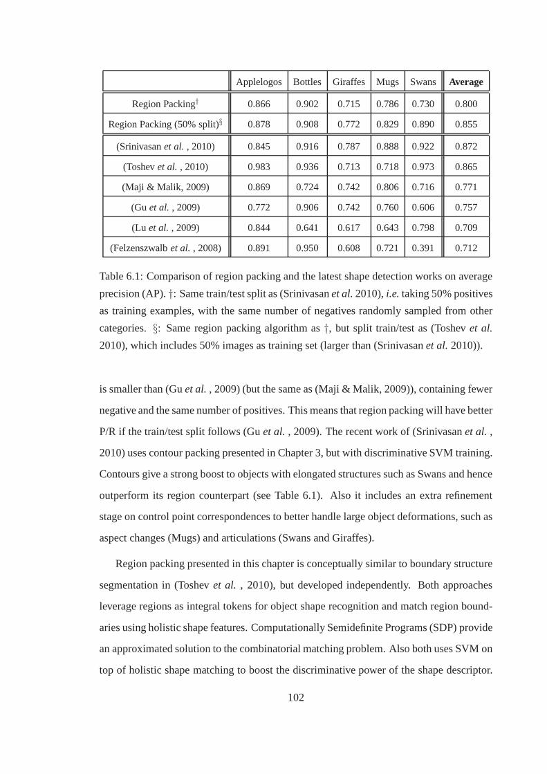
Applelogos Bottles Giraffes Mugs Swans Average

Region Packing† 0.866 0.902 0.715 0.786 0.730 0.800

Region Packing (50% split)§ 0.878 0.908 0.772 0.829 0.890 0.855

(Srinivasanet al. , 2010) 0.845 0.916 0.787 0.888 0.922 0.872

(Toshevet al. , 2010) 0.983 0.936 0.713 0.718 0.973 0.865

(Maji & Malik, 2009) 0.869 0.724 0.742 0.806 0.716 0.771

(Guet al. , 2009) 0.772 0.906 0.742 0.760 0.606 0.757

(Lu et al. , 2009) 0.844 0.641 0.617 0.643 0.798 0.709

(Felzenszwalbet al. , 2008) 0.891 0.950 0.608 0.721 0.391 0.712

Table 6.1: Comparison of region packing and the latest shapedetection works on average

precision (AP).†: Same train/test split as (Srinivasanet al.2010),i.e. taking 50% positives

as training examples, with the same number of negatives randomly sampled from other

categories.§: Same region packing algorithm as†, but split train/test as (Toshevet al.

2010), which includes 50% images as training set (larger than (Srinivasanet al.2010)).

is smaller than (Guet al., 2009) (but the same as (Maji & Malik, 2009)), containing fewer

negative and the same number of positives. This means that region packing will have better

P/R if the train/test split follows (Guet al. , 2009). The recent work of (Srinivasanet al. ,

2010) uses contour packing presented in Chapter 3, but with discriminative SVM training.

Contours give a strong boost to objects with elongated structures such as Swans and hence

outperform its region counterpart (see Table 6.1). Also it includes an extra refinement

stage on control point correspondences to better handle large object deformations, such as

aspect changes (Mugs) and articulations (Swans and Giraffes).

Region packing presented in this chapter is conceptually similar to boundary structure

segmentation in (Toshevet al. , 2010), but developed independently. Both approaches

leverage regions as integral tokens for object shape recognition and match region bound-

aries using holistic shape features. Computationally Semidefinite Programs (SDP) provide

an approximated solution to the combinatorial matching problem. Also both uses SVM on

top of holistic shape matching to boost the discriminative power of the shape descriptor.

102

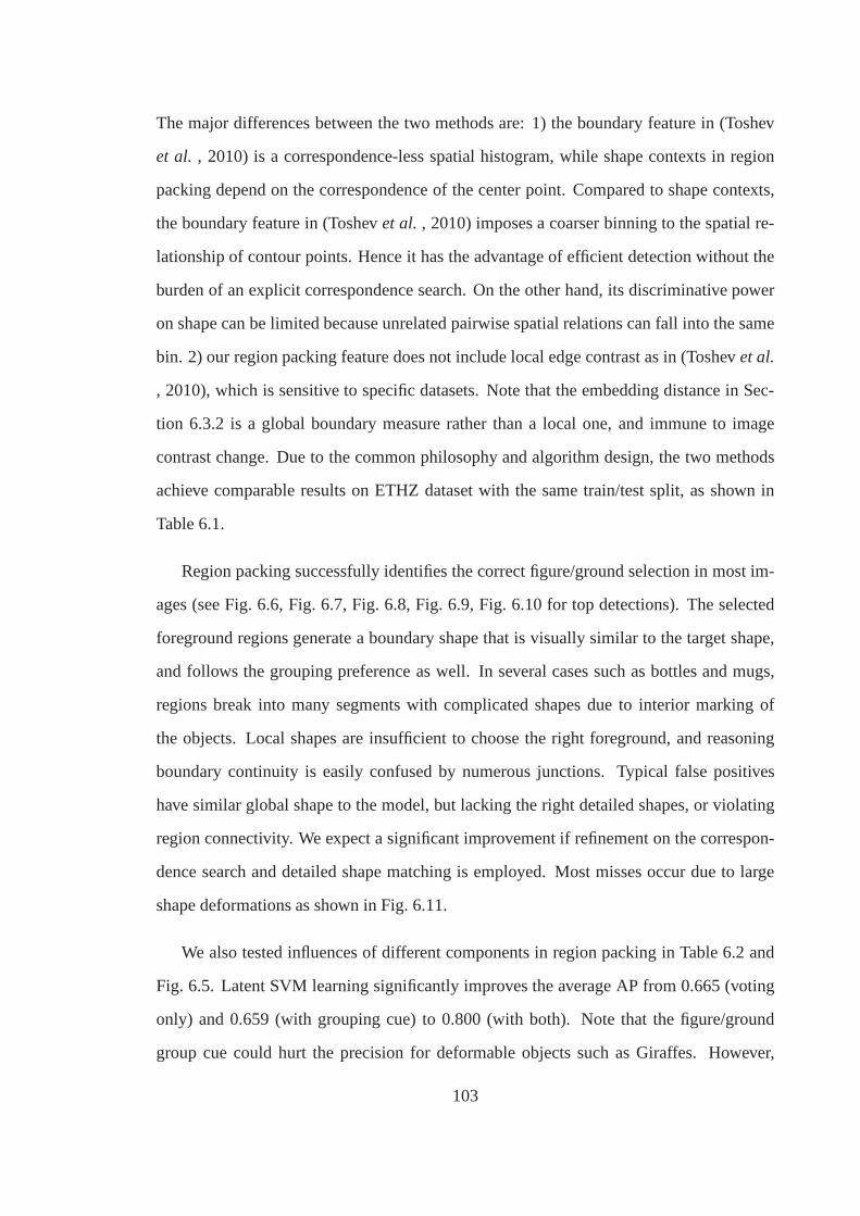
The major differences between the two methods are: 1) the boundary feature in (Toshev

et al. , 2010) is a correspondence-less spatial histogram, while shape contexts in region

packing depend on the correspondence of the center point. Compared to shape contexts,

the boundary feature in (Toshevet al. , 2010) imposes a coarser binning to the spatial re-

lationship of contour points. Hence it has the advantage of efficient detection without the

burden of an explicit correspondence search. On the other hand, its discriminative power

on shape can be limited because unrelated pairwise spatial relations can fall into the same

bin. 2) our region packing feature does not include local edge contrast as in (Toshevet al.

, 2010), which is sensitive to specific datasets. Note that the embedding distance in Sec-

tion 6.3.2 is a global boundary measure rather than a local one, and immune to image

contrast change. Due to the common philosophy and algorithmdesign, the two methods

achieve comparable results on ETHZ dataset with the same train/test split, as shown in

Table 6.1.

Region packing successfully identifies the correct figure/ground selection in most im-

ages (see Fig. 6.6, Fig. 6.7, Fig. 6.8, Fig. 6.9, Fig. 6.10 fortop detections). The selected

foreground regions generate a boundary shape that is visually similar to the target shape,

and follows the grouping preference as well. In several cases such as bottles and mugs,

regions break into many segments with complicated shapes due to interior marking of

the objects. Local shapes are insufficient to choose the right foreground, and reasoning

boundary continuity is easily confused by numerous junctions. Typical false positives

have similar global shape to the model, but lacking the rightdetailed shapes, or violating

region connectivity. We expect a significant improvement ifrefinement on the correspon-

dence search and detailed shape matching is employed. Most misses occur due to large

shape deformations as shown in Fig. 6.11.

We also tested influences of different components in region packing in Table 6.2 and

Fig. 6.5. Latent SVM learning significantly improves the average AP from 0.665 (voting

only) and 0.659 (with grouping cue) to 0.800 (with both). Note that the figure/ground

group cue could hurt the precision for deformable objects such as Giraffes. However,

103

0 0.1 0.2 0.3 0.4 0.5 0.6 0.7 0.8 0.9 10

0.1

0.2

0.3

0.4

0.5

0.6

0.7

0.8

0.9

1

Applelogos

Voting,AP=0.773F/G,AP=0.856F/G+learning,AP=0.866

0 0.1 0.2 0.3 0.4 0.5 0.6 0.7 0.8 0.9 10

0.1

0.2

0.3

0.4

0.5

0.6

0.7

0.8

0.9

1

Bottles


0 0.1 0.2 0.3 0.4 0.5 0.6 0.7 0.8 0.9 10

0.1

0.2

0.3

0.4

0.5

0.6

0.7

0.8

0.9

1

Giraffes


0 0.1 0.2 0.3 0.4 0.5 0.6 0.7 0.8 0.9 10

0.1

0.2

0.3

0.4

0.5

0.6

0.7

0.8

0.9

1

Mugs


0 0.1 0.2 0.3 0.4 0.5 0.6 0.7 0.8 0.9 10

0.1

0.2

0.3

0.4

0.5

0.6

0.7

0.8

0.9

1

Swans


(a) Applelogos (b) Bottles (c) Giraffes (d) Mugs (e) Swans

Figure 6.5: Precision vs. Recall curves (PR).

w/o SVM w/o grouping Full system

Overall AP 0.665 0.659 0.800

Table 6.2: The effect of different factors in region packing.

since the constraint regularizes the region selection, it makes learning feature weights

easier and hence gain significant boost after training.

6.5 Summary

In this chapter, we have proposed a novel feature packing framework using bottom-up

regions to recognize shapes. Starting from fragmented regions, we try to assemble a subset

of them into the model shape such that their overall boundaryshapes are similar. A subset

of regions are holistically matched to the model if they can pack the same set of shape

boundary features as the model. Due to the topological relationship between regions and

their boundaries, the holistic shape matching is formulated as a bipartite graph packing

problem. The combinatorial search of bipartite graph packing can be approximated and

solved efficiently via SDP. We extend the formulation to incorporate various grouping

cues, and unify all these components in the graph partitioning setting. The framework

has shown results on ETHZ Shape Classes comparable with the state-of-the-art region-

based methods, with less reliance on features other than shape. The promising results

are largely attributed to the ability to overcome arbitraryregion fragmentation and utilize

region-based grouping cues.

104

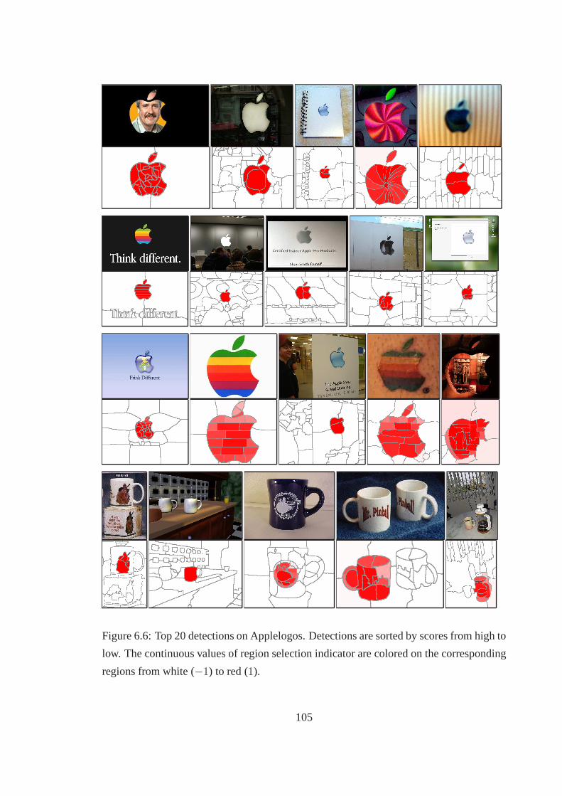
Figure 6.6: Top 20 detections on Applelogos. Detections aresorted by scores from high to

low. The continuous values of region selection indicator are colored on the corresponding

regions from white (−1) to red (1).

105

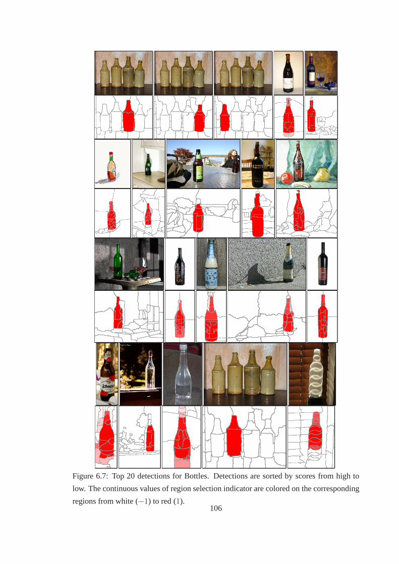
Figure 6.7: Top 20 detections for Bottles. Detections are sorted by scores from high to


regions from white (−1) to red (1).106

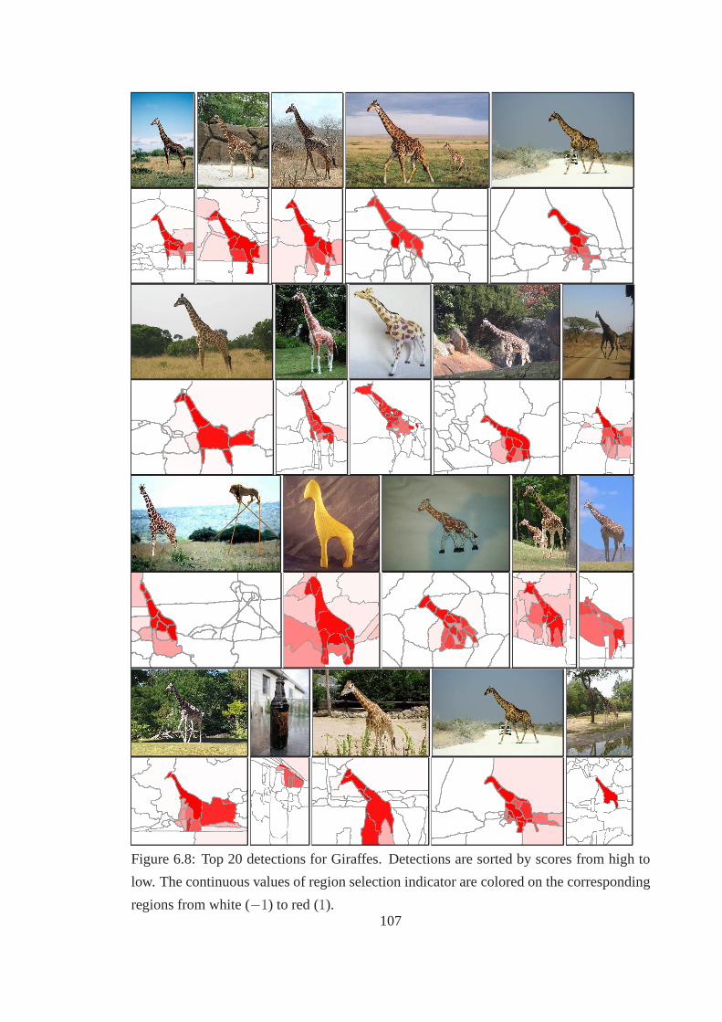
Figure 6.8: Top 20 detections for Giraffes. Detections are sorted by scores from high to


regions from white (−1) to red (1).107

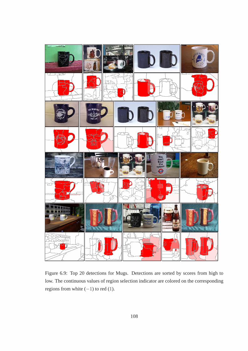
Figure 6.9: Top 20 detections for Mugs. Detections are sorted by scores from high to



108

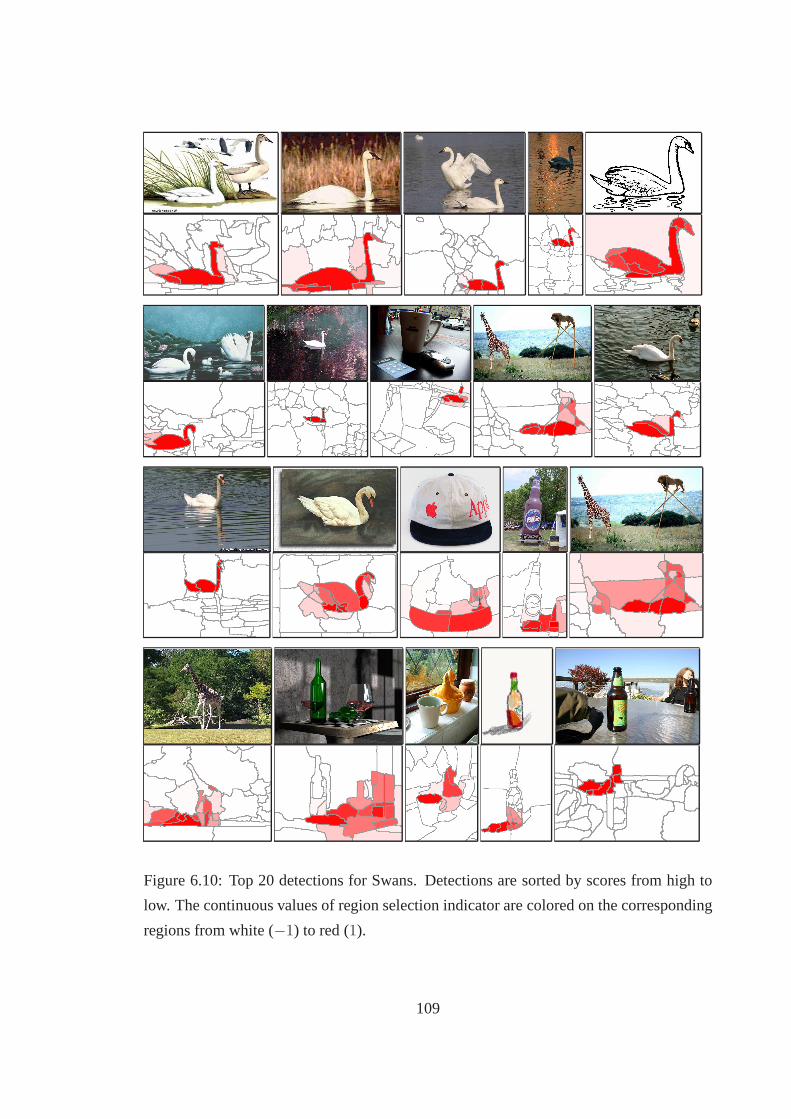
Figure 6.10: Top 20 detections for Swans. Detections are sorted by scores from high to



109

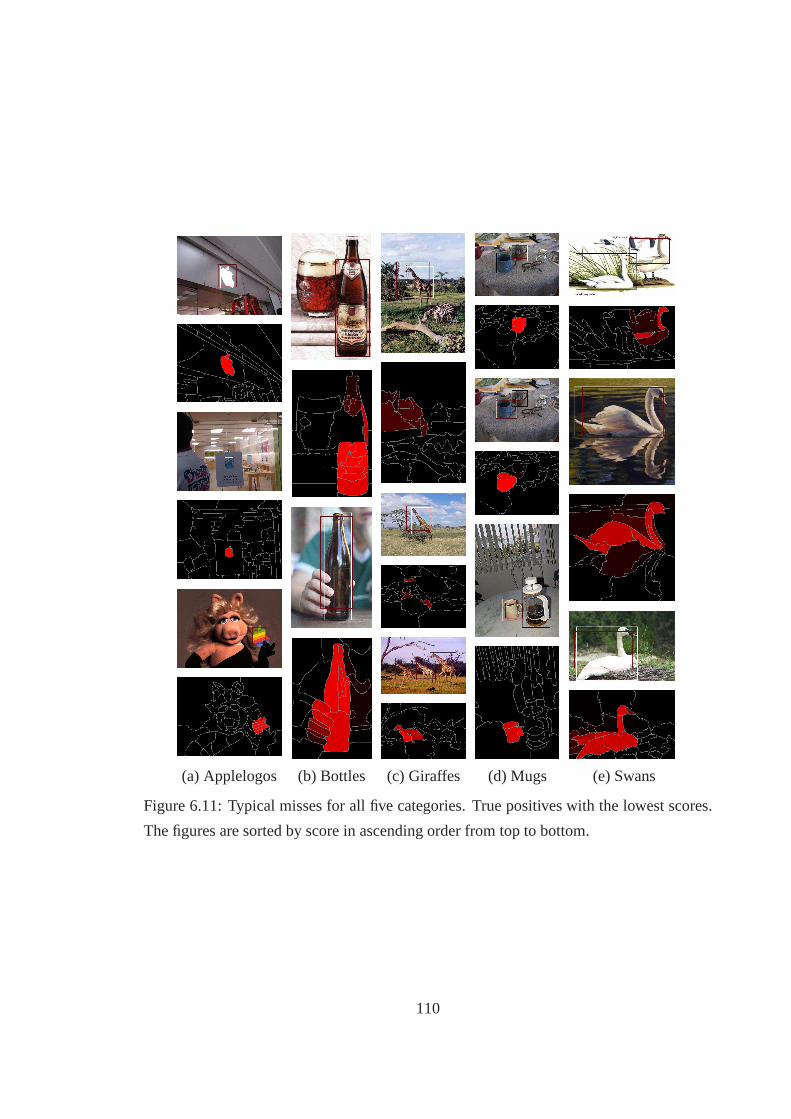
(a) Applelogos (b) Bottles (c) Giraffes (d) Mugs (e) Swans

Figure 6.11: Typical misses for all five categories. True positives with the lowest scores.

The figures are sorted by score in ascending order from top to bottom.

110

Chapter 7

Conclusion

Exploiting global contexts to detect and recognize complexpatterns while keeping the

search computationally tractable has been a fundamental issue not only in computer vi-

sion, but also in the broad area of artificial intelligence. In this thesis, we consider this

problem in the setting of detecting shapes from natural images with various complexities.

Unlike other patterns such as textures which may be locally recognizable, shape is typi-

cally perceived as a whole – it is fundamentally about the global geometric arrangement of

a set of entities. With few distinctive local shape features, reasoning on individual entities

without examining their surroundings is bound to be unreliable.

Traditional contextual models such as Markov Random Fields(MRF) face two diffi-

culties on this problem. First, only short range contextualrelations are usually considered

in these models. Pixels are connected within a small neighborhood, and model parts have

constraints only if they are nearby (e.g.pictorial structures). This limited scope is caused

by either the fact that background can corrupt the long rangerelations, or lacking cues to

generate such constraints. Second, the contextual relations are often restricted to pairwise

constraints to ensure computational tractability. However, most shape configurations can-

not be decomposed into the summation of pairwise checks. Thesimplest case is a straight

line whose valid verification involves at least three points. Any pair of two points can form

a line and therefore does not give any information on the hypothesis. In general, robustly

matching a shape requires simultaneous reasoning over manyentities. In this thesis, we

111

have developed a principled approach that addresses the context issue from the following

aspects:

1. We identifies the underlying generic structures that capture the inherent correlations

of a long sequence of points, independent of the model. Specifically, Chapter 2

introduces a novel topological formulation for grouping contours. The mechanism

is able to extract topologically 1D image contours robust toclutter and broken edges,

and generally applicable to grouping and segmenting data forming a parameterized

structure (i.e.a manifold). Part of the work in Chapter 2 was published in (Zhu et al.

, 2007).

2. The set-to-set matching method we developed in Chapter 3 opens a path towards

utilizing the context arising from a set, going beyond the traditional pairwise con-

straints on tokens. This was made feasible by a holistic shape feature that can be

adjusted on-the-fly according to the context from figure/ground selection. The re-

sulting combinatorial problem of matching can be optimizedand bounded by LP-

based primal-dual algorithms presented in Chapter 4. Part of the work in Chapter 3

was published in (Zhuet al. , 2008; Srinivasanet al. , 2010). The review on primal

dual algorithms in Chapter 4 is based on (Zhu, 2009).

3. Additionally, we are able to incorporate more sophisticated structures into the con-

textual shape reasoning. Chapter 5 extends the holistic approach to match image

contours with an articulation model represented by atree. In Chapter 6, the basic

shape tokens,i.e. regions, do not generate shape features by themselves. It isthe

differenceof a region and its neighbors in terms of figure/ground selection produce

boundaries forming object shapes. This property brings in bipartite graph packing.

We have noticed several future directions worthy of furtherexploration:

1. Interaction between grouping and shape matching. Although the holistic shape rea-

soning requires extraction of discrete, big structures from bottom-up grouping, this

112

does not mean that grouping and shape matching have to be performed in a sequen-

tial, feed-forward way. The feedback from top-down shape matching can potentially

resolve ambiguities in bottom-up grouping. For example, a well matched incom-

plete shape can guide the search for missing segments due to faint boundaries and

leakages. The integration of the decisions on the two processes is preferred.

2. Integration of regions and contours into the packing framework. We have devel-

oped and demonstrated contour packing and region packing separately in Chapter 3

and Chapter 6. Contours express elongated boundary structures while regions cap-

ture boundary closure and figure/ground segregation. The complementary role of

contours and regions suggests that combining the two into a single computational

framework would further reduce false shape detections.

3. Designing better deformable model representation. The tree-based model we used

in Chapter 5 is a special case of AND/OR graph (Zhu & Mumford, 2006), which is

more suitable for representing models with multiple prototypes and occlusions. It is

also important to consider how to exploit features generated from the intermediate

level of AND/OR graph.

4. Finding common shapes in multiple images. In all the computational paradigms, we

dealt with holistic matching between only two shapes. Discovering common shapes

from multiple images would be interesting from both practical and theoretical point

of views. In addition to spatial context contained within each individual image,

context across all the images needs to be investigated for this problem.

5. Extension of primal-dual algorithms to model selection and region packing. We

have merely scratched the surface of employing these ideas to search and bound the

resulting general packing problem. Additional structuressuch as bipartite graph on

the image side and tree or AND/OR graph on the model side are not exploited. We

believe that more efficient combinatorial algorithms and procedures can be designed

by incorporating these new structures into the oracle.

113

Appendix

A.1 Proof of Theorem 2.1

Theorem 2.1 The necessary condition for the critical points (local maxima) of the fol-

lowing optimization problem

maxx∈Cn


xHx(A.1)

is thatx is an eigenvector of

M(∆θ) =1

2(P · e−i∆θ + P T · ei∆θ) (A.2)

Moreover, the corresponding local maximal value is the eigenvalueλ(M(∆θ)).

Proof. Let x = xr + i · xc wherexr andxc are the real and imaginary parts ofx. The

original problem can be rewritten as

maxxr,xc

(xTr Pxr + xT

c Pxc) cos ∆θ + (xTr Pxc − xT

c Pxr) sin ∆θ (A.3)

s.t. xTr xr + xT

c xc = 1 (A.4)

xr, xc ∈ Rn (A.5)

Hence, the Lagrangian has the following form withλ as the multiplier on the constraint:

L = (xTr Pxr + xT

c Pxc) cos ∆θ + (xTr Pxc − xT

c Pxr) sin ∆θ + λ(xTr xr + xT

c xc − 1)

114

By taking derivatives of the Lagrangian, we have

∂L

∂xr= (P T + P ) cos∆θ · xr + (P − P T ) sin ∆θ · xc + 2λxr = 0 (A.6)

∂L

∂xc

= (P T + P ) cos∆θ · xc + (P T − P ) sin∆θ · xr + 2λxc = 0 (A.7)

Setting the above derivatives to0 gives all the local maxima of the original problem

(2.1). Notice thatP is a real matrix, we obtain the following equation by combining

eq. (A.6) and eq. (A.7):

[P + P T

2· cos ∆θ + i · P

T − P

2· sin ∆θ ] · (xr + i · xc) = −λ(xr + i · xc) (A.8)

Thereforex = xr + i · xc is a real eigenvector of matrix:

M(∆θ) =P + P T

2· cos ∆θ + i · P

T − P

2· sin ∆θ (A.9)

=1

2(P · e−i∆θ + P T · ei∆θ) (A.10)

with eigenvalue−λ. Notice thatM(∆θ) is a Hermitian matrix and hence all its eigenval-

ues are real. By substituting eq. (A.6) and eq. (A.7) back to the original cost function we

have

(xTr Pxr + xT

c Pxc) cos∆θ + (xTr Pxc − xT

c Pxr) sin ∆θ = −λ(xTr xr + xT

c xc) = −λ

(A.11)

The local optimal values are exactly the corresponding eigenvalues ofM(∆θ).


First we prove the following lemma:

Lemma 1Pr(i, m) can be expressed in terms of eigenvalues and eigenvectors oftransition

matrixP 1:

Pr(i, m) =∑

λj real

λmj UijVij +

∑

λj complex

Re(λmj UijVij) (A.12)

1To simplify the analysis, we assume thatP is diagonalizable inCn×n and achieve this by perturbingP . For anyǫ ∈ R, there exists diagonalizableQ such that‖P −Q‖ < ǫ.

115

whereλj is thejth eigenvalues ofP andUij is theith entry of thejth right eigenvector

andVij is theith entry of thejth left eigenvector.

Proof. By simple induction one can prove that

Pr(i, m) = (P m)ii (A.13)

Here(P m)ij represents the entry at rowi and columnj.

Consider the eigenvalue decomposition ofP

P = UΣU−1 (A.14)

HereΣ = diag(λ1, ..., λn) andU is a nonsingular complex matrix whose columns are

corresponding eigenvectorsu1, ..., un. Since eigenvectors are not necessarily orthogonal,

U−1 is not equal toUH in general. However, rows ofU−1 are left eigenvectors ofP ,

i.e. (U−1)T = V . The power ofP can be easily computed by

P m = UΣmU−1 (A.15)

We can write(P m)ii as

(P m)ii = (UΣmU−1)ii (A.16)

=∑

j

Uij · λmj · Vij (A.17)

=∑

λj real

λmj UijVij +

∑

λj complex

Re(λmj UijVij) (A.18)

Eq (A.18) comes from the fact thatUij andVij are all real ifλj is real and all complex

eigenvalues appear in pairs.

With Lemma 1, we can easily proveTheorem 2.

Theorem 2.2(Peakness of Random Walk Cycles)R(i, T ) can be computed by the eigen-

values of transition matrixP :

R(i, T ) =

∑j Re(

λTj

1−λTj

· UijVij)∑


(A.19)

116

Image

Model

tt

m m

∑k vk − ∑

k uk

t + m

t + m

C2

C1

wij = aiaj

Cut(C1, C2)

(a) Packing one bin (b) The corresponding graph cut

Figure A.1: Reduction from packing to MaxCut. (a) is a simplecase where there is only

one bin. The red blocks represent image contours nodesI. The green blocks are nodes

for model partsM and the yellow nodes is the fictitious node{V0}. Image or model

background nodes are shaded. (b) shows the corresponding graph cut of the packing.

Proof. FromLemma 1, it is straight forward to get

∞∑

k=1

Pr(i, kT ) =∑

j

Re(λTj /(1− λT

j ) · UijVij) (A.20)

∞∑

k=1

Pr(i, k) =∑

j

Re(1/(1− λj) · UijVij) (A.21)

Finally we have

R(i, T ) =

∑j Re(

λTj

1−λTj

· UijVij)∑


(A.22)


In this section we show that the contour packing problem can be reduced to MaxCut

when the dissimilarity functionDij(·) in eq. (3.7) isL2. This reformulation leads to a

computational solution via SDP, with a proved bound on the optimal cost.

A simple example with one bin

First we start with the simplified case containing one bin only. In this case the bin

contains one single value of feature counts. For convenience, we denote:

• t =∑

i∈SI vi to be the total contribution of selected image contoursSI to the bin;

117

• t =∑

i/∈SI vi to be the contribution fromunselectedcontoursI \ SI ;

• m =∑

i∈SM ui to be the total contribution of selected model partsSM ;

• m =∑

i/∈SI ui to be the contribution fromunselectedmodel partsM\ SM .

With the above notations, optimizing eq. (??) can be reduced to minimizing:

(t−m)2 = (∑

i∈SI

vi −∑

i∈SM

ui)2 (A.23)

We balance the total contributions of the image and model side to the bin by adding a

dummy nodeV0. Without loss of generality, we assume∑

i ui ≥∑

i vi and the contribu-

tion of V0 to the bin is∑

i ui −∑

i vi. V0 can be regarded as a virtual contour which can

neverbe packed. By including this special node, we are ready to establish the connection

between the packing and MaxCut:

Lemma A.1. Set graphGpacking = (V, E, W ) with V = I ∪M∪ {V0} andwij = aiaj ,

where

ai =

vi if Vi ∈ I

ui if Vi ∈M∑

k uk −∑

k vk if Vi = V0


∗ with the best matching cost(t−m)2 in eq. (A.23) is given

by the maximum cut of the packing graphGpacking. If (C1, C2) is the cut withV0 ∈ C2, the


∗ =M∩ C2 (see Fig. A.3).

Proof. Since the total contributions ofI ∪ {V0} andM are the same to the bin, we can

simply includeV0 into I. Any cut (C1, C2) of the graphGpacking with V0 ∈ C2 uniquely

defines the selection onI andM asSI = I ∩ C1 andSM = M∩ C2. Also notice that

C1 = SI ∪ (M\ SM) andC2 = SM ∪ (I \ SI). Recall thatt, t, m andm represent the

total contributions fromSI , I \SI , SM andM\SM respectively. BecauseV0 contributes

to t, we can setc = t + t = m + m.

118

The cut valueCut(C1, C2) can be computed by

Cut(C1, C2) =∑

i∈C1,j∈C2

wij =∑

i∈C1,j∈C2

aiaj

=(∑

i∈C1

ai)(∑

j∈C2

aj) = (t + m)(t + m) (A.24)

∑i∈C1

ai = t + m comes from equalitiesC1 = SI ∪ (M \ SM), t =∑

i∈SI ai and

m =∑

i/∈SM ai. Similarly we can prove∑

j∈C2aj = t + m.

Finally, a simple calculation shows that the cut value and the matching cost sum up to

a constantc2:

(t + m)(t + m) = c2 − (t−m)2

Therefore, minimizing(t − m)2 is equivalent to finding the maximum cut onGpacking,

whose cut value is given by(t + m)(t + m).

Note that without any constraint, the system can choose trivial solution of packing

nothing from image and model. This corresponds to the cut betweenI andM. This

can be alleviated by fixing the model nodes since we know what to pack on the model

side. We also have the freedom of multiple choices on model nodes, which is essential

for articulation model in Section 4.2. These modifications can all be encoded as hard

constraints on the MaxCut.

Reduction of the full problem

Lemma A.1 can be naturally generalized to multiple knapsacks. Each bin inHj intro-

duces an extra node. SetA to be the set of all these nodes. Now we would like to consider

the cut on the graph with nodesI,M andA. This is captured by Theorem 3.1:

Construct a graphGpacking = (V, E, W ) with V = I ∪ M ∪ A and wij = aTi aj ,

where

ai =

V I(:,i) if nodei ∈ I

V M(:,i) if nodei ∈M

(0, ..., 0, |∑k V Iik −

∑k V M

ik |, 0, ..., 0)T if nodei ∈ A

(A.25)

119

HereVI(k, i) is the feature contribution of image segmenti to the histogram bink. V M(k, i)

is defined similarly.V I(:,i) andV M

(:,i) are theith columns ofV I andV M .


∗ with the best matching cost∑

k(tk−mk)2 in eq. (A.23)

is given by the maximum cut of the graphGpacking. If (C1, C2) is the cut withV0 ∈ C2, the


∗ =M∩ C2.

Proof. Let Gpacking = G1 ∪ ... ∪ Gl whereGk’s are graphs induced by bink defined in

Lemma A.1. Applying Lemma A.1 to all these subgraphs.


Theorem A.2. (Littlestone & Warmuth, 1989) (Perturbed Value of the Strategy) LetR =∑

t

∑j yt

jRtj andL =

∑t

∑j yt

jLtj be the cumulative reward and loss of the strategy

using eq. (4.7). The perturbed value of the strategy given byeq. (4.7) is worse than the

performance of best pure strategy only bylog mǫ

, as stated in the following inequality:

maxjVj ≤ exp(ǫ)R− exp(−ǫ)L+

log m

ǫ(A.26)

Proof. Consider the potential functionΦt =∑

j ytj.

On the one hand, we can compute it using the update rule:

Φt =∑

j

ytj

=∑

j

y(0)

t∏

k=1

exp[ǫVkj ] (Update rule (4.7))

=∑

j

exp[ǫ

t∑

k=1

Vkj ] (y(0)

j = 1)

≥ exp[ǫ ·t∑

k=1

Vkj ] (A.27)

Note the above inequality holds for anyj. Therefore,Φt is bounded below by

Φt ≥ exp[ǫ ·maxjVj ] (A.28)

120

On the other hand, we have

yt+1j − yt

j = yt[exp(ǫV tj)− 1]

≤ yt · (ǫV tj) · exp(ǫV t

j)

= yt[ǫ exp(ǫV tj)Rt

j − ǫ exp(ǫV tj)Lt

j]

≤ yt[ǫ exp(ǫ)Rtj − ǫ exp(−ǫ)Lt

j ]

= ytǫV tj

Here V tj = exp(ǫ)Rt

j − exp(−ǫ)Ltj is the “perturbed” version of valueV t

j . The first

inequality holds becauseexp(x)− 1 ≤ x · exp(x) for anyx. The second inequality is due

to the fact thatV tj ∈ [−1, 1].

By summing up the above inequality overj, we have

Φt+1 =∑

j

(yt+1j − yt

j) + Φt

≤∑

j

ytjǫV t

j + Φt

= ǫΦt ·∑

j

ytjV t

j/∑

j

ytj + Φt

= Φt(1 + ǫV t)

≤ Φt · exp(ǫV t) (1 + x ≤ exp(x))

Using induction overt andΦ0 = m, we boundΦt above by

Φt ≤ m · exp(∑

k

ǫVk) (A.29)

Finally combining eq. (A.28), (A.29) yields

ǫ ·maxjVj ≤ log m +

∑

k

ǫVk (A.30)

which is equivalent to eq. (4.8).

121

A.5 Proof of Corollary 4.2

Corollary A.3. (Regret Over Time) IfV tj ∈ [−ρ, ρ] for all j, then we have a bound on the

average valueV/T :

maxj

Vj

T≤ V

T+

ρ log m

ǫT+ ρǫ exp(ǫ) (A.31)

Proof. SinceV tj ∈ [−ρ, ρ], we can substituteV t

j by V tj/ρ and prove the following inequal-

ity for V tj ∈ [−1, 1]:

maxjVj ≤ V +

log m

ǫ+ Tǫ exp(ǫ)

We setRtj = max(0,V t

j) andLtj = max(0,−V t

j), which satisfiesV tj = Rt

j − Ltj.

Under these simplifications, we can apply Theorem 4.1 onV:

maxjVj ≤ V +

log m

ǫ

= V +log m

ǫ+ (exp(ǫ)− 1)R− (exp(−ǫ)− 1)L

≤ V +log m

ǫ+ ǫ exp(ǫ)|V|

≤ V +log m

ǫ+ ǫ exp(ǫ)T

The first inequality uses the fact that|V| = R+L, exp(ǫ)−1 ≤ ǫ exp(ǫ) and1−exp(−ǫ) ≤

ǫ < ǫ exp(ǫ).


Theorem A.4. (Complexity of the Primal Dual Algorithm) Algorithm 2 either declares

that the fractional packing eq. (4.2) is infeasible, or outputs an approximate feasible solu-

tion x satisfying

aTj x− cj ≤ δ (A.32)

for all j = 1, ..., m. The total number of calls to the oracle isO(ρ2δ−2 log m) with ρ =

maxj maxx∈P |fj(x)|.

122

Proof. We build our proof based on Corollary 4.2. First notice that if µt > 0 at some

time t, then the eq. (4.2) is indeed infeasible. Otherwise supposethere existsxt such

thatfj(xt) = aT

j xt − cj ≤ 0 for all j. Becauseyt ≥ 0 throughout the algorithm,µt ≤∑

j ytjfj(x

t) ≤ 0, a contradiction.

Suppose the algorithm runs to the end and outputsx. LetV tj = wtfj(x

t) be the value

incurred by the update. Notice thatV tj ∈ [−1, 1]. By applying Corollary 4.2, we have

maxj

[aTj x− cj ] = max

j

∑t w

t(aTj xt − cj)∑t w

t

= maxj

∑t V t

j∑t w

t

≤ 1∑t wt

[V +log m

ǫ+ ǫT exp(ǫ)]

≤ 1∑t wt

[log m

ǫ+ ǫT exp(ǫ)]

=1

S[log m

ǫ+ ǫT exp(ǫ)]

≤ δ (A.33)

The first inequality uses the fact thatV t = (wt/∑

j ytj)

∑j yt

jfj(xt) = wtµt/

∑j yt

j ≤0 for every t since the oracle never fails. The last inequality is due to the termination

conditionS ≥ 9ρ log m/δ−2, T/S = T/∑

t wt ≤ ρ andǫ = 3δ/ρ.

Therefore,x returned by the algorithm satisfies the approximate feasibility eq. (4.13).

Finally, each time the algorithm collectswt ≥ 1/ρ and it terminates whenS =∑

t wt ≥S ≥ 9ρ log m/δ−2, so the total number of iterations is at mostO(ρ2δ−2 log m).


Theorem A.5. The bipartite region graph packing problem consists in finding an optimal

bipartite subgraphGsub(F, F ) of the region graphG, which minimizes costCp(F, F ) de-

fined in eq. (6.2). It can be reduced to a cardinality constrained and multicriteria cut prob-

lem on a graphG′ associated withR positive edge weight functionsw(1),...,w(R) according

toR criteria. The cardinality constrained and multicriteria cut problem seeks a cutC with

123

cardinality at leastd:∑

Eij∈C 1 ≥ d, and allR criteria are satisfied:∑

Eij∈C w(k)ij ≤ b(k)

for k = 1, 2, ..., R.

Proof. We first transform bipartite region graph packing problem into a simpler linear

form, and notice that the main hurdle is the bipartite graph packing costCp(F, F ) is an

L1-norm. Using a similar technique which converts contour packing into primal-dual

packing in eq. (4.15), we have:

minx,s+,s−

‖V I · x− scM‖1 = 1T[Diag(scM)s+ + Diag(scM)s−] (A.34)

s.t. V Ix− scM = Diag(scM)s+ − Diag(scM)s− (A.35)

x ∈ {0, 1}|E(G)|, s+, s− ∈ [0, 1]m (A.36)

Heres+ ands− are normalized slack variables on the feature bins. Furthermore, this can

be rewritten as:

maxx,s+

V I + 2 · 1TDiag(scM)(1− s+) (A.37)

s.t. V Ix + Diag(scM)(1− s+) ≤ scM (A.38)

x ∈ {0, 1}|E(G)|, s+ ∈ [0, 1]m (A.39)

by substituting the constraint in eq. (A.35) and using the fact thats− is nonnegative. We

can further make the continuous slack variable(1−s+) ∈ [0, 1]m a binary one by splitting

it into units of 1,2,4,...,2ℓ pixels for each bin. Since ultimately the cost is measured as

multiples of a pixel, the binary representation is sufficient to reproduce any integer slack.

We group these slack variables into a single vectors.

If one would like to bound the objective function eq. (A.37),a feasibility problem

arises by changing the objective function into a constraintV I +2·1TDiag(scM)(1−s+) ≥

c for a constantc:

Feasibility(x, s) : V I + 2 · pTs ≥ c (A.40)

V Ix + pTs ≤ scM (A.41)

x ∈ {0, 1}|E(G)|, s ∈ [0, 1]m (A.42)

124

wherepi is the number of pixels included in slacks+i . Now the feasibility problem appears

to be the same as a cardinality constrained and multicriteria cut problem except that the

binary indicatorsx ands have to be defined on graph edges and(x, s) must represent a

cut to the graph.

Construct a graphG′ with additional nodesV (G′) = {Vf , Vb}∪V (G)∪S with follow-

ing specifications: 1) TwoVf ,Vb are the source and sink terminals of the graph representing

foreground and background respectively; 2)V (G) are the nodes from the region graphG

and a node belongs to foreground if on the same side asVf in the cut; 3)S denotes the bin

slack variabless and the slack is applied if on the same side asVf in the cut. Define edge

weight functionsw(i) to beV Iik for edgeEk in G2, andpi for edge betweensi andVb. The

left side of each constraint inFeasibility(x, s) is the sum of weights in a cut onG′.

The above problem is exactly a cardinality constrained and multicriteria cut problem

with cardinality defined by the cost function and criteria defined by the feature bins.

2Unary terms used in Section 6.3 can be represented as edges betweenV (G) and{Vf , Vb}

125

References

ALTER, T. D., & BASRI, RONEN. 1996. Extracting Salient Curves from Images: An

Analysis of the Saliency Network.IEEE Conference on Computer Vision and Pattern

Recognition (CVPR).

AMIR, ARNON, & L INDENBAUM , M ICHAEL. 1998. Grouping-Based Nonadditive Ver-

ification. IEEE Transactions on Pattern Analysis and Machine Intelligence (PAMI),

20(2), 186–192.

AMIT, YALI , & W ILDER, KENNETH. 1997. Joint Induction of Shape Features and Tree

Classifiers.IEEE Transactions on Pattern Analysis and Machine Intelligence (PAMI),

19(11), 1300–1305.

ANDERSEN, E. D., & ANDERSEN, K. D. 2000. The MOSEK interior point optimizer

for linear programming: an implementation of the homogeneous algorithm. Pages

197–232 of: et al., H. FRENK (ed),High Performance Optimization. Dordrecht, The

Netherlands: Kluwer Academic Publishers.

BAI , X., LATECKI , L.J., & LIU , W.Y. 2007. Skeleton Pruning by Contour Partitioning

with Discrete Curve Evolution.IEEE Transactions on Pattern Analysis and Machine

Intelligence (PAMI), 29(3), 449–462.

BARROW, H. G., TENENBAUM, J. M., BOLLES, R. C., & WOLF, H. C. 1977. Paramet-

ric Correspondence and Chamfer Matching: Two New Techniques for Image Match-

ing. International Joint Conference on Artificial Intelligence(IJCAI), 659–663.

126

BASRI, R., & JACOBS, D. W. 1997. Recognition Using Region Correspondences.Inter-

national Journal of Computer Vision (IJCV), 25(2), 145–166.

BELONGIE, SERGE, MALIK , JITENDRA, & PUZICHA , JAN. 2002. Shape Matching and

Object Recognition Using Shape Contexts.IEEE Transactions on Pattern Analysis

and Machine Intelligence (PAMI).

BENTZ, C., COSTA, M. C., DERHY, N., & ROUPIN, F. 2009. Cardinality constrained

and multicriteria (multi)cut problems.J. of Discrete Algorithms, 7(March), 102–111.

BERG, A. C., BERG, T. L., & M ALIK , J. 2005. Shape Matching and Object Recognition

Using Low Distortion Correspondences.IEEE Conference on Computer Vision and

Pattern Recognition (CVPR), I: 26–33.

BIEDERMAN, I. 1985. Human Image Understanding: Recent Research and a Theory.

Computer Vision, Graphics, and Image Processing (CVGIP), 32, 29–73.

BLUM , H. 1967. A Transformation for Extracting new Descriptors of Shape.Pages 362–

380 of: WATHEN-DUNN (ed),Models for the Perception of Speech and Visual Form.

MIT-Press.

BORENSTEIN, E., & ULLMAN , S. 2002. Class-Specific, Top-Down Segmentation.Eu-

ropean Conference on Computer Vision (ECCV).

BOYD, STEPHEN, & VANDENBERGHE, L IEVEN. 2004. Convex Optimization. Cam-

bridge: Cambridge University Press.

BROOKS, R. 1983. Model-Based 3-D Interpretations of 2-D Images.IEEE Transactions

on Pattern Analysis and Machine Intelligence (PAMI), 5(2), 140–150.

BRUGLIERI, MAURIZIO , MAFFIOLI , FRANCESCO, & EHRGOTT, MATTHIAS. 2004.

Cardinality constrained minimum cut problems: complexityand algorithms.Dis-

crete Appl. Math., 137(March), 311–341.

127

CATANZARO , BRYAN , SU, BOR-Y IING , SUNDARAM , NARAYANAN , LEE, YUNSUP,

MURPHY, MARK , & K EUTZER, KURT. 2009. Efficient, High-Quality Image Con-

tour Detection.IEEE International Conference on Computer Vision (ICCV).

COOTES, T. F., TAYLOR, C. J., COOPER, D. H., & GRAHAM , J. 1995. Active Shape

Models: Their Training and Application.Computer Vision and Image Understanding

(CVIU), 61(1), 38–59.

COUR, TIMOTHEE, & SHI , JIANBO. 2007. Solving Markov Random Fields with Spec-

tral Relaxation.Proceedings of the Eleventh International Conference on Artificial

Intelligence and Statistics (AISTATS), 11.

COUR, TIMOTHEE, BENEZIT, FLORENCE, & SHI , JIANBO. 2005. Spectral Segmentation

with Multiscale Graph Decomposition.IEEE Conference on Computer Vision and

Pattern Recognition (CVPR).

DALAL , NAVNEET, & TRIGGS, BILL . 2005. Histograms of Oriented Gradients for

Human Detection.IEEE Conference on Computer Vision and Pattern Recognition

(CVPR), 886–893.

ELDER, J. H., & ZUCKER, S. W. 1996. Computing contour closure.Lecture Notes in

Computer Science, 1064.

FELZENSZWALB, P. F., & MCALLESTER, D. 2006. A Min-Cover Approach for Finding

Salient Curves.IEEE Computer Society Workshop on Perceptual Organizationin

Computer Vision (WPOCV), 185.

FELZENSZWALB, P. F., MCALLESTER, D., & RAMANAN , D. 2008. A discriminatively

trained, multiscale, deformable part model.IEEE Conference on Computer Vision

and Pattern Recognition (CVPR), 1–8.

FELZENSZWALB, PEDRO F., & SCHWARTZ, JOSHUA D. 2007. Hierarchical Matching of

Deformable Shapes.IEEE Conference on Computer Vision and Pattern Recognition

(CVPR).

128

FELZENSZWALB, P.F., & HUTTENLOCHER, D.P. 2005. Pictorial Structures for Object

Recognition.International Journal of Computer Vision (IJCV).

FERRARI, V ITTORIO, JURIE, FREDERIC, & SCHMID , CORDELIA. 2007a. Accurate Ob-

ject Detection with Deformable Shape Models Learnt from Images.IEEE Conference

on Computer Vision and Pattern Recognition (CVPR).

FERRARI, V ITTORIO, FEVRIER, L, JURIE, FREDERIC, & SCHMID , CORDELIA. 2007b.

Groups of Adjacent Contour Segments for Object Detection.IEEE Transactions on

Pattern Analysis and Machine Intelligence (PAMI).

FISCHER, BERND, & BUHMANN , JOACHIM M. 2003. Path-Based Clustering for Group-

ing of Smooth Curves and Texture Segmentation.IEEE Transactions on Pattern

Analysis and Machine Intelligence (PAMI), 25(4), 513–518.

GALLEGUILLOS , CAROLINA , BABENKO, BORIS, RABINOVICH , ANDREW, & BE-

LONGIE, SERGE. 2008. Weakly Supervised Object Recognition and Localization

with Stable Segmentations.European Conference on Computer Vision (ECCV).

GDALYAHU , YORAM, & WEINSHALL , DAPHNA. 1999. Flexible Syntactic Matching of

Curves and Its Application to Automatic Hierarchical Classification of Silhouettes.

IEEE Transactions on Pattern Analysis and Machine Intelligence (PAMI).

GOEMANS, M. X., & W ILLIAMSON , D.P. 1995. Improved Approximation Algorithms

for Maximum Cut and Satisfiability Problems Using Semidefinite Programming.

Journal of the ACM, 42, 1115–1145.

GORELICK, LENA, GALUN , MEIRAV, SHARON, EITAN , BASRI, RONEN, & BRANDT,

ACHI. 2006. Shape Representation and Classification Using the Poisson Equation.

IEEE Transactions on Pattern Analysis and Machine Intelligence (PAMI), 28(12),

1991–2005.

GRIMSON, ERIC. 1986. The Combinatorics of Local Constraints in Model-Based Recog-

nition and Localization from Sparse Data.JACM: Journal of the ACM, 33.

129

GRIMSON, W. E. L., & LOZANO-PEREZ, T. 1987. Localizing Overlapping Parts by

Searching the Interpretation Tree.IEEE Transactions on Pattern Analysis and Ma-

chine Intelligence (PAMI), 9, 469–482.

GU, CHUNHUI , L IM , JOSEPH J., ARBELAEZ, PABLO , & M ALIK , JITENDRA. 2009.

Recognition using Regions.IEEE Conference on Computer Vision and Pattern

Recognition (CVPR).

GUPTA, ABHINAV, & DAVIS, LARRY S. 2008. Beyond Nouns: Exploiting Prepositions

and Comparative Adjectives for Learning Visual Classifiers. European Conference

on Computer Vision (ECCV), 5302, 16–29.

HAN , F., & ZHU, S. C. 2009. Bottom-Up/Top-Down Image Parsing with Attribute Gram-

mar.IEEE Transactions on Pattern Analysis and Machine Intelligence (PAMI), 31(1),

59–73.

HUTTENLOCHER, KLANDERMAN , & RUCKLIDGE. 1993. Comparing Images Using the

Hausdorff Distance.IEEE Transactions on Pattern Analysis and Machine Intelli-

gence (PAMI), 15.

JACOBS, DAVID W. 1996. Robust and Efficient Detection of Salient Convex Groups.

IEEE Transactions on Pattern Analysis and Machine Intelligence (PAMI), 18(1), 23–

37.

JIANG , H., & M ARTIN , D. R. 2008. Global pose estimation using non-tree models.IEEE

Conference on Computer Vision and Pattern Recognition (CVPR), 1–8.

JIANG , HAO, DREW, MARK S., & LI , ZE-NIAN . 2007. Matching by Linear Program-

ming and Successive Convexification.IEEE Transactions on Pattern Analysis and

Machine Intelligence (PAMI), 29(6), 959–975.

KESELMAN, YAKOV, & D ICKINSON, SVEN J. 2005. Generic Model Abstraction from

Examples.IEEE Transactions on Pattern Analysis and Machine Intelligence (PAMI),

27(7), 1141–1156.

130

KHANDEKAR, ROHIT. 2004. Lagrangian Relaxation Based Algorithms for Convex Pro-

gramming Problems. Ph.D. thesis, IIT Delhi.

KOFFKA, KURT. 1935.Principles of Gestalt Psychology.

KOHLER, W. 1929.Gestalt psychology. New York: Liveright.

LAMDAN , Y., SCHWARTZ, J. T., & WOLFSON, H. J. 1990. Affine Invariant Model-

Based Object Recognition.IEEE Transactions on Robotics and Automation, 6, 578–

589.

LATECKI , LONGIN JAN , LU, CHENGEN, SOBEL, MARC, & BAI , X IANG. 2008. Mul-

tiscale Random Fields with Application to Contour Grouping. Advances in Neural

Information Processing Systems (NIPS), 913–920.

LEE, MUN WAI , & COHEN, ISAAC. 2004. Proposal Maps Driven MCMC for Estimat-

ing Human Body Pose in Static Images.IEEE Conference on Computer Vision and

Pattern Recognition (CVPR).

LEIGHTON, T., MAKEDON, F., PLOTKIN , S., STEIN, C., TARDOS, E., & TRAGOUDAS,

S. 1991. Fast Approximation Algorithms for MulticommodityFlow Problems.23rd

Annual ACM Symposium on Theory of Computing (STOC), 101–111.

LEORDEANU, MARIUS, HEBERT, MARTIAL , & SUKTHANKAR , RAHUL . 2007. Beyond

Local Appearance: Category Recognition from Pairwise Interactions of Simple Fea-

tures.IEEE Conference on Computer Vision and Pattern Recognition(CVPR).

LEYMARIE , F.F., & LEVINE, M.D. 1992. Simulating the Grassfire Transform Using an

Active Contour Model.IEEE Transactions on Pattern Analysis and Machine Intelli-

gence (PAMI), 14(1), 56–75.

L I , L.J., SOCHER, R., & FEI FEI, L. 2009. Towards total scene understanding: Classi-

fication, annotation and segmentation in an automatic framework. IEEE Conference

on Computer Vision and Pattern Recognition (CVPR), 2036–2043.

131

L ING, HAIBIN , & JACOBS, DAVID W. 2005. Using the Inner-Distance for Classification

of Articulated Shapes.IEEE International Conference on Computer Vision (ICCV).

L ITTLESTONE, & WARMUTH. 1989. The Weighted Majority Algorithm.FOCS: IEEE

Symposium on Foundations of Computer Science (FOCS).

LOWE, DAVID G. 2004. Distinctive Image Features from Scale-Invariant Keypoints.In-

ternational Journal of Computer Vision (IJCV), 60(2), 91–110.

LU, CHENGEN, LATECKI , LONGIN JAN , ADLURU, NAGESH, YANG, X INGWEI, &

L ING, HAIBIN . 2009. Shape Guided Contour Grouping with Particle Filters. IEEE

International Conference on Computer Vision (ICCV).

MAHAMUD , S., WILLIAMS , L., THORNBER, K., & X U, K. 2003. Segmentation of

multiple salient closed contours from real images.IEEE Transactions on Pattern

Analysis and Machine Intelligence (PAMI).

MAIRE, M., ARBELAEZ, P., FOWLKES, C., & MALIK , J. 2008. Using contours to detect

and localize junctions in natural images.

MAJI, S., & MALIK , J. 2009. Object detection using a max-margin Hough transform.

CVPR, 1038–1045.

MALISIEWICZ , TOMASZ, & EFROS, ALEXEI A. 2008. Recognition by Association via

Learning Per-exemplar Distances.IEEE Conference on Computer Vision and Pattern

Recognition (CVPR), June.

MARTIN , DAVID R., FOWLKES, CHARLESS, TAL , DORON, & M ALIK , JITENDRA.

2001. A Database of Human Segmented Natural Images and its Application to Eval-

uating Segmentation Algorithms and Measuring Ecological Statistics.IEEE Interna-

tional Conference on Computer Vision (ICCV), 416–425.

MEDIONI, G. G., & GUY, G. 1993. Inferring Global Perceptual Contours from Local

Features.Image Understanding Workshop (IUW).

132

MEILA , MARINA , & SHI , JIANBO. 2000. Learning Segmentation by Random Walks.

Advances in Neural Information Processing Systems (NIPS), 873–879.

MORI, G. 2005. Guiding Model Search Using Segmentation.IEEE International Con-

ference on Computer Vision (ICCV).

MORI, GREG, REN, X IAOFENG, EFROS, ALEXEI A., & M ALIK , JITENDRA. 2004a. Re-

covering Human Body Configurations: Combining Segmentation and Recognition.

IEEE Conference on Computer Vision and Pattern Recognition(CVPR), 326–333.

MORI, GREG, REN, X IAOFENG, EFROS, ALEXEI A., & M ALIK , JITENDRA. 2004b.

Recovering human body configurations: combining segmentation and recognition.

IEEE Conference on Computer Vision and Pattern Recognition(CVPR).

NESTEROV, Y. E., & NEMIROVSKY, A. S. 1993.Interior Point Polynomial Methods in

Convex Programming : Theory and Algorithms. SIAM Publishing.

NEVATIA , R., & BINFORD, T. O. 1977. Description and Recognition of Curved Objects.

Artificial Intelligence, 8(1), 77–98.

PALMER, S. 1999.Vision Science: Photons to Phenomenology. MIT Press.

PELEG, S., & ROSENFELD, A. 1981. A Min-Max Medial Axis Transformation.IEEE

Transactions on Pattern Analysis and Machine Intelligence(PAMI), 3(2), 208–210.

PENTLAND , A. P. 1986. Perceptual Organization and the Representation of Natural Form.

Artificial Intelligence, 28, 293–331.

PLOTKIN , SERGE A., SHMOYS, DAVID B., & TARDOS, EVA . 1995. Fast Approximation

Algorithms for Fractional Packing and Covering Problems.Mathematics of Opera-

tions Research, 20, 257–301.

RAMANAN , DEVA. 2007. Learning to parse images of articulated bodies.Advances in

Neural Information Processing Systems (NIPS).

133

REN, X IAOFENG, BERG, ALEXANDER C., & MALIK , JITENDRA. 2005a. Recovering

human body configurations using pairwise constraints between parts.IEEE Interna-

tional Conference on Computer Vision (ICCV).

REN, X IAOFENG, FOWLKES, CHARLESS, & M ALIK , JITENDRA. 2005b. Scale-Invariant

Contour Completion Using Conditional Random Fields.IEEE International Confer-

ence on Computer Vision (ICCV), 1214–1221.

RONFARD, REMI , SCHMID , CORDELIA, & TRIGGS, BILL . 2002. Learning to Parse

Pictures of People.European Conference on Computer Vision (ECCV).

SARKAR, SUDEEP, & SOUNDARARAJAN, PADMANABHAN . 2000. Supervised Learn-

ing of Large Perceptual Organization: Graph Spectral Partitioning and Learning Au-

tomata. IEEE Transactions on Pattern Analysis and Machine Intelligence (PAMI),

22(5), 504–525.

SHARON, E., & MUMFORD, D. 2006. 2D-Shape Analysis Using Conformal Mapping.

International Journal of Computer Vision, 70(1), 55–75.

SHI , J., & MALIK , J. 2000. Normalized Cuts and Image Segmentation.IEEE Transac-

tions on Pattern Analysis and Machine Intelligence (PAMI), 22(8), 888–905.

SHOTTON, J. D. J., BLAKE , A., & CIPOLLA , R. 2008. Multiscale Categorical Object

Recognition Using Contour Fragments.IEEE Transactions on Pattern Analysis and

Machine Intelligence (PAMI), 30(7), 1270–1281.

SHOTTON, JAMIE , BLAKE , ANDREW, & CIPOLLA , ROBERTO. 2005. Contour-Based

Learning for Object Detection.IEEE International Conference on Computer Vision

(ICCV).

SIDDIQI , K., SHOKOUFANDEH, A., DICKINSON, S. J., & ZUCKER, S. W. 1999. Shock

Graphs and Shape Matching.International Journal of Computer Vision, 35(1), 13–

32.

134

SRINIVASAN , PRAVEEN, & SHI , JIANBO. 2007. Bottom-up Recognition and Parsing of

the Human Body.IEEE Conference on Computer Vision and Pattern Recognition

(CVPR).

SRINIVASAN , PRAVEEN, ZHU, QIHUI , & SHI , JIANBO. 2010. Many-to-one Contour

Matching for Describing and Discriminating Object Shape.IEEE Conference on

Computer Vision and Pattern Recognition (CVPR).

STURM, J. F. 1999. Using SeDuMi 1.02, a MATLAB toolbox for optimization over

symmetric cones.Optimization Methods and Software, 11, 625–653.

TAYLOR, CAMILLO J., & BHUSNURMATH, ARVIND. 2008. Solving Image Registration

Problems Using Interior Point Methods.European Conference on Computer Vision

(ECCV), October, 638–651.

TODOROVIC, S., & AHUJA, N. 2008. Region-Based Hierarchical Image Matching.In-

ternational Journal of Computer Vision (IJCV), 78(1), 47–66.

TORRALBA, A., RUSSELL, B. C., & YUEN, J. 2009. LabelMe: online image annotation

and applications.MIT CSAIL Technical Report.

TOSHEV, ALEXANDER, TASKAR, BEN, & DANIILIDIS , KOSTAS. 2010. Object Detec-

tion via Boundary Structure Segmentation.IEEE Conference on Computer Vision

and Pattern Recognition (CVPR).

ULLMAN , S. 1996.High-Level Vision: Object Recognition and Visual Cognition. MIT

Press.

ULLMAN , S., & SHASHUA, A. 1988. Structural Saliency: The Detection of Globally

Salient Structures Using a Locally Connected Network.MIT AI Memo.

VAIDYA , PRAVIN M. 1996. A new algorithm for minimizing convex functions over con-

vex sets.Math. Program., 73(3), 291–341.

135

VAZIRANI , V. V. 2004.Approximation Algorithms.Springer.

WANG, L IMING , SHI , JIANBO , SONG, GANG, & SHEN, I-FAN. 2007. Object Detection

Combining Recognition and Segmentation.Asian Conference on Computer Vision

(ACCV).

WANG, SONG, KUBOTA, TOSHIRO, SISKIND , JEFFREY MARK , & WANG, JUN. 2005.

Salient Closed Boundary Extraction with Ratio Contour.IEEE Transactions on Pat-

tern Analysis and Machine Intelligence (PAMI).

WERTHEIMER, M. 1938. Principles of perceptual organisation.In: ELLIS, W. H. (ed),

Source Book of Gestalt Psychology.

WRIGHT, STEPHEN J. 1997.Primal-dual interior-point methods. Philadelphia, PA, USA:

Society for Industrial and Applied Mathematics.

YOUNG, NEAL E. 1995. Randomized rounding without solving the linear program.SODA

’95: Proceedings of the sixth annual ACM-SIAM symposium on Discrete algorithms,

170–178.

YU, STELLA X., & SHI , JIANBO. 2003. Multiclass Spectral Clustering.IEEE Interna-

tional Conference on Computer Vision (ICCV), 313–319.

ZAHN , C. T., & ROSKIES, R. S. 1972. Fourier descriptors for plane closed curves.IEEE

Transactions on Computing.

ZHANG, JIAYONG , LUO, JIEBO, COLLINS, ROBERT, & L IU , YANXI . 2006. Body Lo-

calization in Still Images Using Hierarchical Models and Hybrid Search.IEEE Con-

ference on Computer Vision and Pattern Recognition (CVPR).

ZHU, QIHUI . 2009. Primal Dual Combinatorial Algorithms.CIS WPE-II Report, Univer-

sity of Pennsylvania.

ZHU, QIHUI , SONG, GANG, & SHI , JIANBO. 2007. Untangling Cycles for Contour

Grouping.IEEE International Conference on Computer Vision (ICCV).

136

ZHU, QIHUI , WANG, L IMING , WU, YANG, & SHI , JIANBO. 2008. Contour Context

Selection for Object Detection: A Set-to-Set Contour Matching Approach.European

Conference on Computer Vision (ECCV).

ZHU, SONG-CHUN, & M UMFORD, DAVID . 2006. A stochastic grammar of images.

Foundations and Trends in Computer Graphics and Vision, 2(4), 259–362.

137

Documents

SHAPE DETECTION BY PACKING CONTOURS Qihui Zhu