Shape and Symmetry Induction for 3D Objects

Shubham Tulsiani1, Abhishek Kar1, Qixing Huang2, Joao Carreira1 and Jitendra Malik1

1University of California, Berkeley 2Toyota Technological Institute at Chicago1{shubhtuls, akar, carreira, malik}@eecs.berkeley.edu 2huangqx@ttic.edu

Abstract

Actions as simple as grasping an object or navigatingaround it require a rich understanding of that object’s 3Dshape from a given viewpoint. In this paper we repurposepowerful learning machinery, originally developed for ob-ject classification, to discover image cues relevant for re-covering the 3D shape of potentially unfamiliar objects. Wecast the problem as one of local prediction of surface nor-mals and global detection of 3D reflection symmetry planes,which open the door for extrapolating occluded surfacesfrom visible ones. We demonstrate that our method is ableto recover accurate 3D shape information for classes of ob-jects it was not trained on, in both synthetic and real images.

“What specifies an object are invariants that arethemselves ‘formless’”

J.J. Gibson

1. IntroductionIn this paper we develop a method for understanding the

3D shape of an unfamiliar object from a single image. Ourmethod recovers a 2.5D shape representation by densely la-beling normals of object surfaces visible in the image. Wetarget the remaining 0.5D – the shape of occluded surfaces– by inferring shape self-similarities. As one small step inthis direction, we introduce the task of detecting the orien-tation of any planes of reflection symmetry in the 3D objectshape.

Recovering 3D object shape from a single image isclearly an ill-posed problem and requires assumptions tobe made about the shape. The problem of reconstructingfamiliar categories has seen some success, but there strong3D priors can be learned from training data [6, 20]. Theproblem of reconstructing shapes for previously unseen cat-egories is more subtle and coming up with the right pri-ors seems critical, in particular for recovering occluded sur-faces. We pursue patterns of self-similarity in 3D shape

Figure 1: Given a single image of a novel object, our modelinduces a pixel-wise labeling of its surface normals (right)and predicts the orientations of all 3D planes of reflectionsymmetry (center).

given just the image, hoping these will allow filling in oc-cluded geometry with carefully placed copies of visible ge-ometry. We define an entry-level version of the problem:detecting the 3D orientation of planes of reflection symme-try.

Both components of our approach rely heavily on learn-ing large nonlinear classifiers end-to-end, which has be-come an effective solution to many vision problems, but notyet for 3D object shape reconstruction from a single image.This is due, in part, to technical and logistical difficultiesinvolved in creating large datasets of images of objects withaligned 3D shapes [48, 5].

In this work we leverage synthetic data, and resort to newlarge-scale shape collections where ground truth symme-try planes and surface orientations can be accurately com-puted. We then render these models and use the imagespaired with the symmetry and normal labels to learn Con-volutional Neural Network (CNN) [13, 27] based systemsfor symmetry prediction (Section 3) and normal estimation(Section 4). We show qualitative results on real images andempirically demonstrate the ability of our models to inducethese predictions accurately for novel objects (Section 5).

1

arX

iv:s

ubm

it/14

1414

7 [

cs.C

V]

25

Nov

201

5

2. Related WorkRecovering an object’s surface geometry from a single

image is an ill-posed problem in general – e.g. a same im-age can be caused by different configurations of surface ge-ometry, reflectance and lighting conditions. This problemhas been studied from many different perspectives, whichwe will roughly divide here into physics-based and predic-tive shape inference. These two paradigms, together withprior work on symmetry detection and learning from CADmodel datasets are briefly summarized below.

Physics-based Shape Inference Given an image, thepreference for any particular 3D shape depends strongly onthe type of priors imposed. Physics-based approaches, suchas early shape from shading techniques [18], aimed to opti-mize shape using variational formulations with regularizersthat encoded strong assumptions about albedo and illumi-nation. Modern approaches such as SIRFS [3] extend theseby using richer priors and additionally reasoning over re-flectances in the solution space.

Predictive Shape Inference. The other commonparadigm for shape inference is through supervised learn-ing techniques that leverage training data to boost inferenceresults. Early work on predicting depth (and/or surfacenormals) utilized graphical models [17, 38] and more recentwork have improved performance via hierarchical featureextractors [10]. These previous approaches, however, havefocused on inferring scene-level information which differsfrom our goal of perceiving the shape of objects.

Predicting object pose is another task for which manylearning-based methods have been developed. Traditionalapproaches focused on particular instances and used explicit3D models [19], but the task has recently evolved into theprediction of category-level pose [45, 36, 14]. Category-specific pose prediction models have still the inconveniencethat they do not generalize to novel object categories andrequire large amounts of labeled data for each of their train-ing categories. Recently, Tulsiani et al. [44] showed thattreating pose as an attribute [11, 26] and training a pre-diction system accordingly can enable prediction for unfa-miliar classes. Our work aims for a similar generalizationto arbitrary objects, but the symmetry and surface orienta-tion representations we infer are much more general anddetailed.

Learning from CAD Model Collections. There has beena growing trend of using 3D CAD model renderings to aidcomputer vision algorithms. The key advantage of these ap-proaches is that it is easy to obtain labeled training data atscale. Examples include approaches for aligning 3D mod-els to images [2, 28], object detection [35] and pose estima-

tion [41]. In this work, we apply this idea to normal estima-tion and symmetry detection - both easily obtained from 3Dmodels.

3. Symmetry Prediction

”Symmetry is what we see at a glance; based on thefact that there is no reason for any difference.”

- Blaise Pascal, Pensees

Most real-world shapes possess symmetries. For exam-ple, all object categories available in popular datasets suchas PASCAL VOC and Microsoft COCO exhibit at least bi-lateral reflection symmetry. Symmetry detection providescues into the elongation modes and 3D orientation of ob-jects which can influence perceived shape (as illustrated byErnst Mach square/diamond famous example [34]) and isconjectured to aid grouping [23] and recognition [46] in hu-man vision. Symmetry-based approaches such as Blum’sMedial Axis Transform [4] spawned entire subcommunities[39] devoted to their development.

Symmetry is however now rarely pursued in practicalvision systems, perhaps because too much emphasis hasbeen placed on“retinal” symmetries – symmetries in planarshapes, that are only moderately distorted when projectedinto an image. Most objects are not planar and their symme-tries can be widely deformed after projecting on to imagesdue to the angle relative to the camera and the geometry ofcentral projection. Consequently, we deviate from the exist-ing techniques for detecting retinal symmetrical structureswhich seek dense correspondences across feature points,aiming to detect subsets of correspondences that can be re-alized by the underlying structures [29, 7, 30]. Instead, wepresent a learning-based framework to directly detect theunderlying 3D symmetries for an object.

We propose to infer representations similar to those ofexisting approaches that rely on 3D shape inputs [33] ordepth images [43, 37] - but we aim to do so from a singleRGB image. In fact, we leverage existing approaches fordetecting 3D symmetries in 3D meshes in order to obtainground truth symmetries. We can then frame a supervisedlearning problem using rendered images of these shapes asinput. We describe our symmetry extraction, symmetry pre-diction formulation and learning framework below.

Extracting Symmetries from Shapes. We follow theprocedure outlined by Mitra et al. [33] to extract the globalreflectional symmetries given a shape. We sample the shapeuniformly to correct for any biased sampling in the originalmesh points. We then consider many symmetry plane hy-potheses, parametrized as (n, b) where the points satisfyingn · x = b lie on the plane, and iteratively refine each hy-pothesis via ICP between original and reflected points. We

2

finally discard planes that do not fit the sampled points welland additionally suppress duplicate planes with very simi-lar orientations. We refer the reader to [33] for the exactmathematical formulation.

Formulation. Given an image I , we aim to predict thesymmetry planes of the underlying 3D object. Since theexact placement of a plane only assumes a meaning oncewe have inferred a reconstruction for the object and is notwell defined given a single image, we focus on inferring theorientations of the underlying symmetry planes. LetN rep-resent the space of unit norm 3D orientation vectors. Wefirst discretize this space via approximately uniform sam-ples on the unit sphere [42] {n1, · · · , nK}. Our learningtask is modeled as a multilabel classification where we aimto learn a mapping f ′ s.t. f(I) ∈ {0, 1}K and f(I)[k] = 1iff nk is a correct discretization for some symmetry orien-tation of the underlying 3D object.

Learning. As mentioned earlier, we rely on a large shapecollection to learn prediction of symmetries. We also usea rendering engine E which, given a shape model S anda model rotation R yields a rendered image E(S,R). Toobtain training data for our task, we repeatedly sample ashape S belonging to some object category c ∈ C from theshape collection and detect the underlying reflectional sym-metry planes {Pi = (ni, bi)} as described above. We thensample a model pose from a view distribution V and obtainthe rendered image E(S,R). The symmetry orientationsunderlying the 3D shape of the rendered image ({R ∗ ni})are computed by rotating the symmetry orientations of theshape S. These orientations are discretized as into orien-tation bins described above to obtain a label l ∈ {0, 1}K .The pair (E(S,R), l) forms one training exemplar for ourproblem. We sample models and views repeatedly to gener-ate the training data - the exact details are described in theexperiments.

Given the training set constructed above, we train a CNNto predict symmetries given a single image. More con-cretely, we use an Alexnet [24] based architecture with Koutputs in the last layer and use a sigmoid cross entropyloss to enforce the outputs to represent log-probability ofthe corresponding orientation being a symmetry plane forthe underlying 3D object. Note that the system is trainedin a category-agnostic way ı.e. unlike common detectionand pose prediction systems [45, 41] , we share output unitsacross all object categories c ∈ C. This implicitly enforcesthe CNN based symmetry prediction system to exploit sim-ilarities across object classes and learn common represen-tations that may be useful for generalizing to novel objects.Our experiments empirically demonstrate that the systemwe describe is indeed capable of predicting symmetries forobjects belonging to a category c /∈ C.

4. Surface Normal EstimationThe importance of perceiving the surface layout was

highlighted by Gibson as early as 1950 [15]. These ideaswere grounded more computationally as Marr’s 2.5D sketchrepresentations [32]. Koenderink, Van Doorn and Kapperslater demonstrated [22] the ability of humans to recoversurface orientations from pictures and shaded objects. Allthese seminal works, perceptual as well as computational,emphasized the importance of perceiving surface orienta-tions as an integral part of perception.

Single-image depth [10, 38, 21] and surface normal[12, 9, 47] prediction using CNNs has shown promise whendealing with the shape of scenes. Scenes exhibit strong reg-ularities: the ground and the ceiling is horizontal, the wallsare vertical. Here we demonstrate that these models canbe leveraged to label the much more complex normals ofobject surfaces. We describe our formulation and learningprocedure below.

Formulation. Our aim is to learn a model that is capa-ble of constructing a mapping from pixels to orientationsgiven an image I(·, ·). The desired output, given the inputimage I is a spatial orientation function N(·, ·) such thatN(x, y) is the surface orientation of the point in the under-lying 3D shape that is projected at pixel (x, y) in the givenimage. Instead of directly predicting an orientation n ∈ Nat each spatial location, we follow a formulation motivatedby Koenderink’s experiment where the subjects were ableto reconstruct a dense sampling of surface orientations inimages using an element from discrete set of gauge figuresplaced at every location. This discretization of surface ori-entations has been previously successfully leveraged [25]for estimating surface normals of a scene. Our intuition isthat this approach combined with CNN architectures thathave shown rapid recent progress for pixelwise classifica-tion tasks e.g. semantic segmentation can yield promisingresults in the domain of object shape perception.

Operationally, similar to our approach for symmetryplane orientations, we discretize the space of visible sur-face orientations into K discrete bins using approximatelyuniform samples over the half unit sphere [42]. The goalfor normal estimation is to then learn a function approxi-mation f s.t f(I) = N where N(x, y) assigns the correctorientation bin for the 3D point projected at (x, y).

Learning. Our data generation process is similar to thetask of symmetry prediction described previously. We usea rendering engine E which, given a shape model S and amodel pose R yields a rendered image E(S,R) and addi-tionally provides a surface orientation image N(S,R). Wefirst sample a category c from training classes C and then ashape S. A random view R is sampled from a view distri-

3

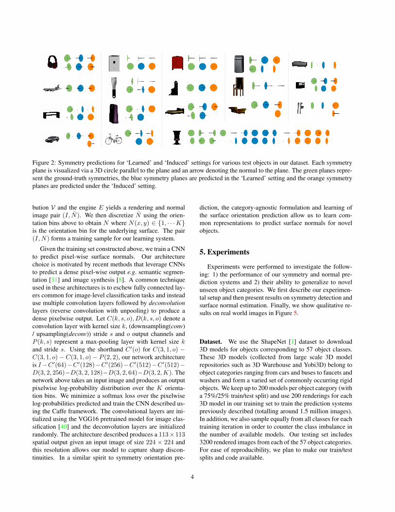
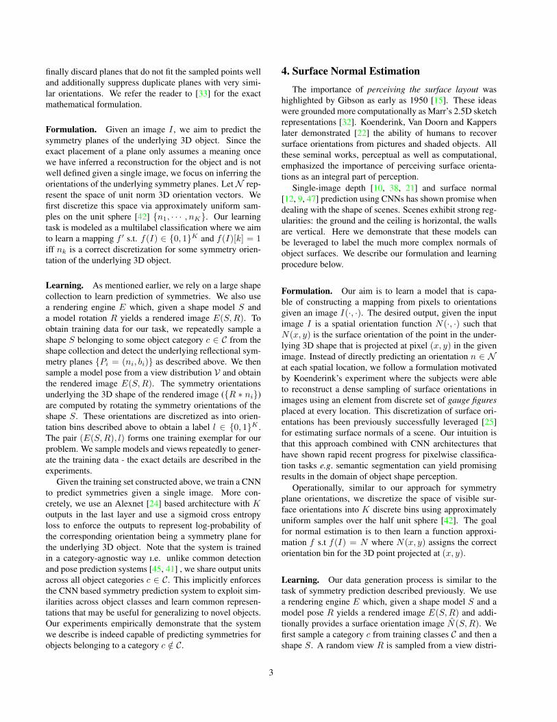
Figure 2: Symmetry predictions for ‘Learned’ and ‘Induced’ settings for various test objects in our dataset. Each symmetryplane is visualized via a 3D circle parallel to the plane and an arrow denoting the normal to the plane. The green planes repre-sent the ground-truth symmetries, the blue symmetry planes are predicted in the ‘Learned’ setting and the orange symmetryplanes are predicted under the ‘Induced’ setting.

bution V and the engine E yields a rendering and normalimage pair (I, N). We then discretize N using the orien-tation bins above to obtain N where N(x, y) ∈ {1, · · ·K}is the orientation bin for the underlying surface. The pair(I,N) forms a training sample for our learning system.

Given the training set constructed above, we train a CNNto predict pixel-wise surface normals. Our architecturechoice is motivated by recent methods that leverage CNNsto predict a dense pixel-wise output e.g. semantic segmen-tation [31] and image synthesis [8]. A common techniqueused in these architectures is to eschew fully connected lay-ers common for image-level classification tasks and insteaduse multiple convolution layers followed by deconvolutionlayers (reverse convolution with unpooling) to produce adense pixelwise output. Let C(k, s, o), D(k, s, o) denote aconvolution layer with kernel size k, (downsampling(conv)/ upsampling(deconv)) stride s and o output channels andP (k, s) represent a max-pooling layer with kernel size kand stride s. Using the shorthand C ′(o) for C(3, 1, o) −C(3, 1, o)− C(3, 1, o)− P (2, 2), our network architectureis I−C ′(64)−C ′(128)−C ′(256)−C ′(512)−C ′(512)−D(3, 2, 256)−D(3, 2, 128)−D(3, 2, 64)−D(3, 2,K). Thenetwork above takes an input image and produces an outputpixelwise log-probability distribution over the K orienta-tion bins. We minimize a softmax loss over the pixelwiselog-probabilities predicted and train the CNN described us-ing the Caffe framework. The convolutional layers are ini-tialized using the VGG16 pretrained model for image clas-sification [40] and the deconvolution layers are initializedrandomly. The architecture described produces a 113× 113spatial output given an input image of size 224 × 224 andthis resolution allows our model to capture sharp discon-tinuities. In a similar spirit to symmetry orientation pre-

diction, the category-agnostic formulation and learning ofthe surface orientation prediction allow us to learn com-mon representations to predict surface normals for novelobjects.

5. Experiments

Experiments were performed to investigate the follow-ing: 1) the performance of our symmetry and normal pre-diction systems and 2) their ability to generalize to novelunseen object categories. We first describe our experimen-tal setup and then present results on symmetry detection andsurface normal estimation. Finally, we show qualitative re-sults on real world images in Figure 5.

Dataset. We use the ShapeNet [1] dataset to download3D models for objects corresponding to 57 object classes.These 3D models (collected from large scale 3D modelrepositories such as 3D Warehouse and Yobi3D) belong toobject categories ranging from cars and buses to faucets andwashers and form a varied set of commonly occurring rigidobjects. We keep up to 200 models per object category (witha 75%/25% train/test split) and use 200 renderings for each3D model in our training set to train the prediction systemspreviously described (totalling around 1.5 million images).In addition, we also sample equally from all classes for eachtraining iteration in order to counter the class imbalance inthe number of available models. Our testing set includes3200 rendered images from each of the 57 object categories.For ease of reproducibility, we plan to make our train/testsplits and code available.

4

Figure 3: Precision-Recall plots for symmetry detectionunder ‘Induced’ and ‘Learned’ settings for representativeclasses.

Viewpoint Variability. The viewing angle for an ob-ject can be described using three euler angles - azimuth(φ ∈ (−180, 180]), elevation(ϕ ∈ (−180, 180]) and cyclo-rotation(ψ ∈ (−90, 90]). Objects, however, tend to followcertain view distributions (e.g. we rarely see cars from thebottom). In particular, the primary variation in viewing an-gle for objects in natural scenes is along the azimuth. Toaccount for this, we sample views uniformly from a set ofmore natural views VN = {φ ∈ (−180, 180]} × {ϕ ∈[0, 10]} × {ψ ∈ [0, 0]}. It is, however, also importantto handle objects seen from arbitrary views. We there-fore also train and test our models under a more diverseview sampling from VD = {φ ∈ (−180, 180]} × {ϕ ∈[0, 50]} × {ψ ∈ [−30, 30]} to analyze the prediction andinduction performance under more challenging settings.

Induction Splits. A primary aim of our experimentalevaluation is to analyze the induction ability of our systemacross novel object classes. For this analysis, we randomlypartitioned the object classes C in the ShapeNet dataset intwo disjoint sets CA and CB - the categories in each setare listed in the appendix. For both the shape predictiontasks we study - normal and symmetry prediction, we train3 models with the same hyper-parameters. One model istrained on the entire set of classes C and two models overCA and CB respectively. This allows us to empirically esti-mate the induction performance for a class c ∈ (CA or CB)by comparing the performance of the systems trained over

Figure 4: Analysis of performance gap (in AP θs ) for ob-ject categories between ‘Induced’ and ‘Learned’ settings forsymmetry prediction.

Mean AP θs Setting

Viewpoint Sampling Learned Induced RandomVN 0.69 0.58 0.32VD 0.59 0.47 0.07

Table 1: Mean performance across classes for symmetryprediction.

C and (CB or CA) respectively. In all the experiments de-scribed below, we report numbers under both the ‘Learned’and ‘Induced’ settings. The ‘Learned’ setting denotes theperformance of our system when trained using all objectclasses and the ‘Induced’ setting indicates our performancewhen, for each object class we use the system trained onthe set of classes (CA or CB) not containing the class underconsideration.

5.1. Symmetry Prediction

Evaluation Criterion. Since the task we address is nota standard one, we need to decide on evaluation metrics.In the related task of pose prediction, the common prac-tice is to measure the deviation between predicted and an-notated pose [45, 41]. Symmetries, however, do not lendthemselves to a similar analysis because there can be mul-tiple of them and consequently, a symmetry prediction sys-tem would yield multiple symmetry hypotheses with vary-ing confidences. In that respect, our task perhaps has morein common with object detection - given an image with avariable number of symmetry planes (c.f . objects), a pre-diction system outputs a few distinct hypotheses from thecontinuous space of plane orientations (c.f . bounding boxlocations). We therefore adapt the standard object detectionAverage Precision (AP) metric for our task.

5

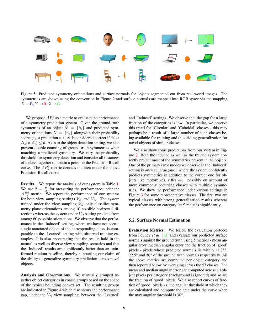
Figure 5: Predicted symmetry orientations and surface normals for objects segmented out from real world images. Thesymmetries are shown using the convention in Figure 2 and surface normals are mapped into RGB space via the mappingX →B, Y →R, Z →G.

We proposeAP θs as a metric to evaluate the performanceof a symmetry prediction system. Given the ground-truthsymmetries of an object N = {ni} and predicted sym-metry orientations N = {nj} alongwith their probabilityscores pj , a prediction n ∈ N is considered correct if ∃i s.t∆s(n, ni) ≤ θ. Akin to the object detection setting, we alsoprevent double counting of ground-truth symmetries whenmatching a predicted symmetry. We vary the probabilitythreshold for symmetry detection and consider all instancesof a class together to obtain a point on the Precision-Recallcurve. The AP θs metric denotes the area under the abovePrecision-Recall curve.

Results. We report the analysis of our system in Table 1.We use θ = π

18 for measuring the performance under theAP θs metric. We report the performance of our systemsfor both view sampling settings VN and VD. The systemtrained under the view sampling VN only classifies sym-metry plane orientations among 10 possible horizontal di-rections whereas the system under VD setting predicts fromamong 60 possible orientations. We observe that the perfor-mance in the ‘Induced’ setting, where we have not seen asingle annotated object of the corresponding class, is com-parable to the ‘Learned’ setting with observed training ex-amples. It is also encouraging that the results hold in thenatural as well as diverse view sampling scenarios and thatthe ‘Induced’ results are significantly better than an unin-formed random baseline, thereby supporting our claim ofthe ability to generalize symmetry prediction across novelobjects.

Analysis and Observations. We manually grouped to-gether object categories in coarse groups based on the shapeof the typical bounding convex set. The resulting groupsare indicated in Figure 4 which also shows the performancegap, under the VN view sampling, between the ‘Learned’

and ‘Induced’ settings. We observe that the gap for a largefraction of the categories is low. In particular, we observethis trend for ’Circular’ and ’Cuboidal’ classes - this mayperhaps be a result of a large number of such classes be-ing available for training and thus aiding generalization fornovel objects of similar classes.

We also show some predictions from our system in Fig-ure 2. Both the induced as well as the trained system cor-rectly predict most of the symmetries present in the objects.One of the primary error modes we observe in the ’Induced’setting is over-generalization where the system confidentlypredicts symmetries in addition to the correct one for ob-jects like motorbikes, rifles etc., possibly on account ofmore commonly occurring classes with multiple symme-tries. We show the performance under various settings inFigure 3 for some representative classes. The first two aretypical classes with strong generalization results whereasthe performance on category ‘car’ reduces significantly.

5.2. Surface Normal Estimation

Evaluation Metrics. We follow the evaluation protocolfrom Fouhey et al. [12] and evaluate our predicted surfacenormals against the ground truth using 5 metrics - mean an-gular error, median angular error and the fraction of ‘good’pixels - pixels whose predicted normals lie within 11.25◦,22.5◦ and 30◦ of the ground truth normals respectively. Allthe above metrics are computed per object category andthen reported below by averaging across the 57 classes. Themean and median angular error are computed across all ob-ject pixels per category (background is ignored) and so arethe fraction of ‘good’ pixels. We also report curves of frac-tion of ‘good’ pixels vs. the angular threshold at which theyare calculated and compute the area under the curve whenthe max angular threshold is 30◦.

6

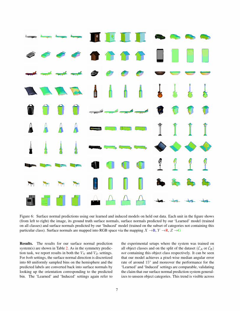
Figure 6: Surface normal predictions using our learned and induced models on held out data. Each unit in the figure shows(from left to right) the image, its ground truth surface normals, surface normals predicted by our ‘Learned’ model (trainedon all classes) and surface normals predicted by our ‘Induced’ model (trained on the subset of categories not containing thisparticular class). Surface normals are mapped into RGB space via the mapping X →B, Y →R, Z →G

Results. The results for our surface normal predictionsystem(s) are shown in Table 2. As in the symmetry predic-tion task, we report results in both the VN and VD settings.For both settings, the surface normal direction is discretizedinto 60 uniformly sampled bins on the hemisphere and thepredicted labels are converted back into surface normals bylooking up the orientation corresponding to the predictedbin. The ‘Learned’ and ‘Induced’ settings again refer to

the experimental setups where the system was trained onall object classes and on the split of the dataset (CA or CB)not containing this object class respectively. It can be seenthat our model achieves a pixel-wise median angular errorrate of around 15◦ and moreover the performance for the‘Learned’ and ‘Induced’ settings are comparable, validatingthe claim that our surface normal prediction system general-izes to unseen object categories. This trend is visible across

7

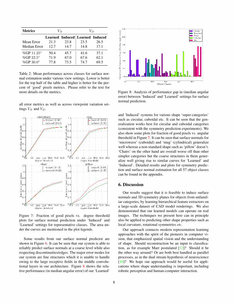
Metrics VN VD

Learned Induced Learned InducedMean Error 21.3 23.8 23.5 26.5Median Error 12.7 14.7 14.8 17.1

%GP 11.25◦ 50.4 45.7 41.6 37.1%GP 22.5◦ 71.9 67.0 67.6 62.1%GP 30.0◦ 77.8 73.5 74.7 69.5

Table 2: Mean performance across classes for surface nor-mal estimation under various view settings. Lower is betterfor the top half of the table and higher is better for the per-cent of ‘good’ pixels metrics. Please refer to the text formore details on the metrics.

all error metrics as well as across viewpoint variation set-tings VN and VD.

Figure 7: Fraction of good pixels vs. degree thresholdplots for surface normal prediction under ‘Induced’ and‘Learned’ settings for representative classes. The area un-der the curves are mentioned in the plot legends.

Some results from our surface normal predictor areshown in Figure 6. It can be seen that our system is able toreliably predict surface normals at a coarse level while alsorespecting discontinuities/edges. The major error modes forour system are fine structures which it is unable to handleowing to the large receptive fields in the middle convolu-tional layers in our architecture. Figure 8 shows the rela-tive performance (in median angular error) of our ‘Learned’

Figure 8: Analysis of performance gap in (median angularerror) between ‘Induced’ and ‘Learned’ settings for surfacenormal prediction.

and ‘Induced’ systems for various shape ‘super-categories’such as circular, cuboidal etc. It can be seen that the gen-eralization works best for circular and cuboidal categories(consistent with the symmetry prediction experiments). Wealso show some plots for fraction of good pixels vs. angularthreshold in Figure 7. It can be seen that surface normals for‘microwave’ (cuboidal) and ‘mug’ (cylindrical) generalizewell whereas a non-standard shape such as ‘pillow’ doesn’t.‘Chairs’ on the other hand are overall worse off than othersimpler categories but the coarse structures in them gener-alize well giving rise to similar curves for ‘Learned’ and‘Induced’. Detailed results and plots for symmetry predic-tion and surface normal estimation for all 57 object classescan be found in the appendix.

6. Discussion

Our results suggest that it is feasible to induce surfacenormals and 3D symmetry planes for objects from unfamil-iar categories, by learning hierarchical feature extractors ona large-scale dataset of CAD model renderings. We alsodemonstrated that our learned models can operate on realimages. The techniques we present here can in principlealso be applied to predicting other shape properties such aslocal curvature, rotational symmetries etc.

Our approach connects modern representation learningapproaches with the spirit of the pioneers in computer vi-sion, that emphasized spatial vision and the understandingof shape. Should reconstruction be an input to classifica-tion, as for example Marr postulated [32]? Should it bethe other way around? Or are both best handled as parallelprocesses, as in the dual stream hypothesis of neuroscience[16]? We hope our approach would be useful for appli-cations where shape understanding is important, includingrobotic perception and human-computer interaction.

8

AcknowledgementsThis work was supported in part by NSF Award IIS-

1212798 and ONR MURI-N00014-10-1-0933. ShubhamTulsiani was supported by the Berkeley fellowship. JoaoCarreira was supported by the Portuguese Science Foun-dation, FCT, under grant SFRH/BPD/84194/2012. QixingHuang thanks the gift awards from Adobe and Intel. Wegratefully acknowledge NVIDIA corporation for GPU do-nations towards this research.

References[1] Shapenet. http://www.shapenet.org. 4, 11

[2] M. Aubry, D. Maturana, A. Efros, B. Russell, andJ. Sivic. Seeing 3d chairs: exemplar part-based 2d-3d alignment using a large dataset of cad models. InCVPR, 2014. 2

[3] J. T. Barron and J. Malik. Shape, illumination, andreflectance from shading. TPAMI, 2015. 2

[4] H. Blum. A transformation for extracting new descrip-tors of shape. In Proc. Models for the Perception ofSpeech and Visual Form, 1967. 2

[5] J. Carreira, S. Vicente, L. Agapito, and J. Batista. Lift-ing object detection datasets into 3d. 2015. 1

[6] T. J. Cashman and A. W. Fitzgibbon. What shape aredolphins? building 3d morphable models from 2d im-ages. IEEE Transactions on Pattern Analysis and Ma-chine Intelligence, 2012. 1

[7] D. Ceylan, N. J. Mitra, Y. Zheng, and M. Pauly. Cou-pled structure-from-motion and 3d symmetry detec-tion for urban facades. ACM Trans. Graph., 2014. 2

[8] A. Dosovitskiy and T. Brox. Inverting convolutionalnetworks with convolutional networks. arXiv preprintarXiv:1506.02753, 2015. 4

[9] D. Eigen and R. Fergus. Predicting depth, surface nor-mals and semantic labels with a common multi-scaleconvolutional architecture. In ICCV, 2015. 3

[10] D. Eigen, C. Puhrsch, and R. Fergus. Depth map pre-diction from a single image using a multi-scale deepnetwork. In NIPS, 2014. 2, 3

[11] A. Farhadi, I. Endres, D. Hoiem, and D. Forsyth. De-scribing objects by their attributes. In CVPR, 2009.2

[12] D. F. Fouhey, A. Gupta, and M. Hebert. Data-driven3D primitives for single image understanding. InICCV, 2013. 3, 6

[13] K. Fukushima. Neocognitron: A self-organizing neu-ral network model for a mechanism of pattern recog-nition unaffected by shift in position. Biological Cy-bernetics, 1980. 1

[14] A. Ghodrati, M. Pedersoli, and T. Tuytelaars. Is 2dinformation enough for viewpoint estimation? InBMVC, 2014. 2

[15] J. J. Gibson. The perception of the visual world. 1950.3

[16] M. A. Goodale and A. D. Milner. Separate visualpathways for perception and action. Trends in neu-rosciences, 15(1):20–25, 1992. 8

[17] D. Hoiem, A. A. Efros, and M. Hebert. Automaticphoto pop-up. In SIGGRAPH, 2005. 2

[18] B. K. Horn. Obtaining shape from shading informa-tion. In Shape from shading, pages 123–171. MITpress, 1989. 2

[19] D. P. Huttenlocher and S. Ullman. Recognizing solidobjects by alignment with an image. IJCV, 1990. 2

[20] A. Kar, S. Tulsiani, J. Carreira, and J. Malik.Category-specific object reconstruction from a singleimage. In CVPR, 2015. 1

[21] K. Karsch, C. Liu, and S. B. Kang. Depthtrans-fer: Depth extraction from video using non-parametricsampling. Pattern Analysis and Machine Intelligence,IEEE Transactions on, 2014. 3

[22] J. J. Koenderink, A. J. Van Doorn, and A. M. Kappers.Pictorial surface attitude and local depth comparisons.Perception & Psychophysics, 58(2):163–173, 1996. 3

[23] K. Koffka. Principles of Gestalt psychology, vol-ume 44. Routledge, 2013. 2

[24] A. Krizhevsky, I. Sutskever, and G. E. Hinton. Im-agenet classification with deep convolutional neuralnetworks. In NIPS, 2012. 3

[25] L. Ladicky, B. Zeisl, and M. Pollefeys. Discrimi-natively trained dense surface normal estimation. InECCV. 2014. 3

[26] C. H. Lampert, H. Nickisch, and S. Harmeling. Learn-ing to detect unseen object classes by between-classattribute transfer. In CVPR, 2009. 2

[27] Y. LeCun, B. Boser, J. Denker, D. Henderson, R. E.Howard, W. Hubbard, and L. D. Jackel. Backpropaga-tion applied to hand-written zip code recognition. InNeural Computation, 1989. 1

[28] J. J. Lim, H. Pirsiavash, and A. Torralba. ParsingIKEA Objects: Fine Pose Estimation. In ICCV, 2013.2

[29] J. Liu and Y. Liu. Curved reflection symmetry de-tection with self-validation. In Asian Conference onComputer Vision(ACCV), 2010. 2

[30] Y. Liu, H. Hel-Or, C. S. Kaplan, and L. J. V.Gool. Computational symmetry in computer visionand computer graphics. Foundations and Trends inComputer Graphics and Vision, 2010. 2

9

[31] J. Long, E. Shelhamer, and T. Darrell. Fully convolu-tional networks for semantic segmentation. In CVPR,2015. 4

[32] D. Marr. Vision: A computational approach, 1982. 3,8

[33] N. J. Mitra, L. Guibas, and M. Pauly. Symmetrization.SIGGRAPH, 2007. 2

[34] S. E. Palmer. Vision science: Photons to phenomenol-ogy. MIT press Cambridge, MA, 1999. 2

[35] X. Peng, B. Sun, K. Ali, and K. Saenko. Exploring in-variances in deep convolutional neural networks usingsynthetic images. CoRR, abs/1412.7122, 2014. 2

[36] B. Pepik, M. Stark, P. Gehler, and B. Schiele. Teach-ing 3d geometry to deformable part models. In CVPR,2012. 2

[37] J. Rock, T. Gupta, J. Thorsen, J. Gwak, D. Shin, andD. Hoiem. Completing 3d object shape from onedepth image. In CVPR, 2015. 2

[38] A. Saxena, M. Sun, and A. Y. Ng. Make3d: Learning3d scene structure from a single still image. PAMI,2009. 2, 3

[39] K. Siddiqi, A. Shokoufandeh, S. J. Dickinson, andS. W. Zucker. Shock graphs and shape matching. In-ternational Journal of Computer Vision, 35(1):13–32,1999. 2

[40] K. Simonyan and A. Zisserman. Very deep convo-lutional networks for large-scale image recognition.CoRR, abs/1409.1556, 2014. 4

[41] H. Su, C. R. Qi, Y. Li, and L. J. Guibas. Renderfor cnn: Viewpoint estimation in images using cnnstrained with rendered 3d model views. In ICCV, 2015.2, 3, 5

[42] R. Swinbank and R. James Purser. Fibonacci grids:A novel approach to global modelling. Quar-terly Journal of the Royal Meteorological Society,132(619):1769–1793, 2006. 3

[43] S. Thrun and B. Wegbreit. Shape from symmetry. InICCV, 2005. 2

[44] S. Tulsiani, J. Carreira, and J. Malik. Pose inductionfor novel object categories. In ICCV, 2015. 2

[45] S. Tulsiani and J. Malik. Viewpoints and keypoints. InCVPR, 2015. 2, 3, 5

[46] T. Vetter and T. Poggio. Linear object classes andimage synthesis from a single example image. Pat-tern Analysis and Machine Intelligence, IEEE Trans-actions on, 19(7):733–742, 1997. 2

[47] X. Wang, D. F. Fouhey, and A. Gupta. Designing deepnetworks for surface normal estimation. In CVPR,2015. 3

[48] Y. Xiang, R. Mottaghi, and S. Savarese. Beyondpascal: A benchmark for 3d object detection in thewild. In Applications of Computer Vision (WACV),2014 IEEE Winter Conference on, pages 75–82. IEEE,2014. 1

10

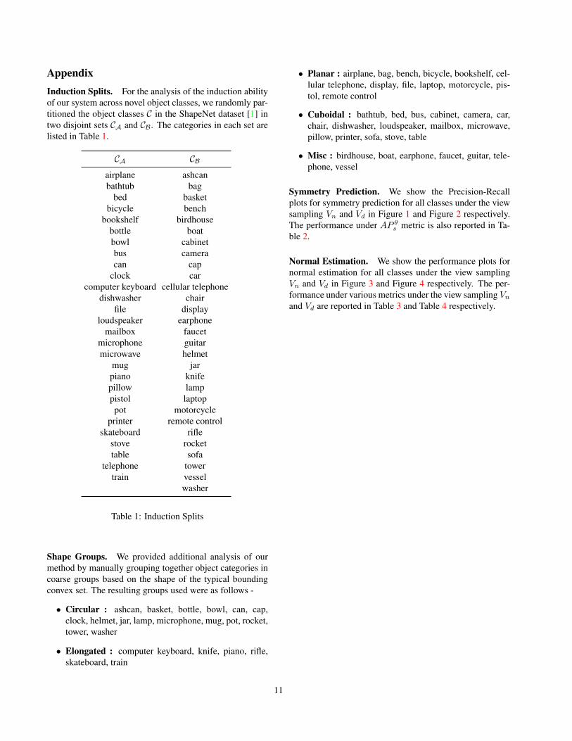
AppendixInduction Splits. For the analysis of the induction abilityof our system across novel object classes, we randomly par-titioned the object classes C in the ShapeNet dataset [1] intwo disjoint sets CA and CB. The categories in each set arelisted in Table 1.

CA CBairplane ashcanbathtub bag

bed basketbicycle bench

bookshelf birdhousebottle boatbowl cabinetbus cameracan cap

clock carcomputer keyboard cellular telephone

dishwasher chairfile display

loudspeaker earphonemailbox faucet

microphone guitarmicrowave helmet

mug jarpiano knifepillow lamppistol laptoppot motorcycle

printer remote controlskateboard rifle

stove rockettable sofa

telephone towertrain vessel

washer

Table 1: Induction Splits

Shape Groups. We provided additional analysis of ourmethod by manually grouping together object categories incoarse groups based on the shape of the typical boundingconvex set. The resulting groups used were as follows -

• Circular : ashcan, basket, bottle, bowl, can, cap,clock, helmet, jar, lamp, microphone, mug, pot, rocket,tower, washer

• Elongated : computer keyboard, knife, piano, rifle,skateboard, train

• Planar : airplane, bag, bench, bicycle, bookshelf, cel-lular telephone, display, file, laptop, motorcycle, pis-tol, remote control

• Cuboidal : bathtub, bed, bus, cabinet, camera, car,chair, dishwasher, loudspeaker, mailbox, microwave,pillow, printer, sofa, stove, table

• Misc : birdhouse, boat, earphone, faucet, guitar, tele-phone, vessel

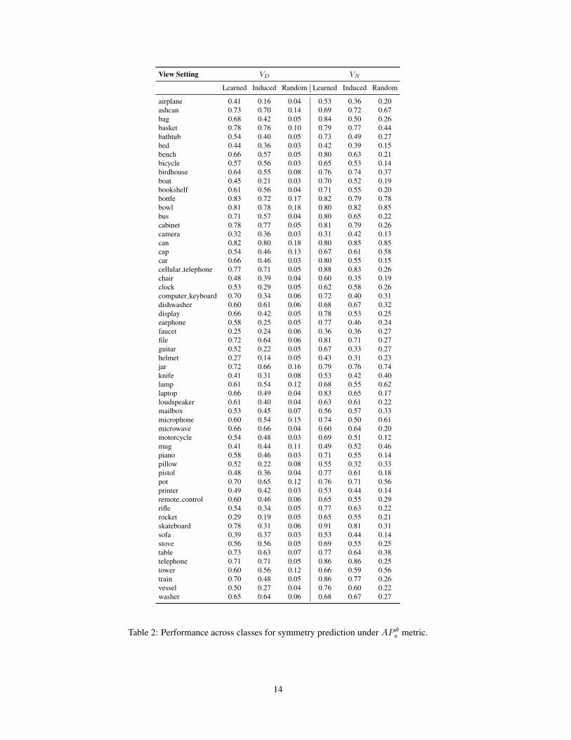
Symmetry Prediction. We show the Precision-Recallplots for symmetry prediction for all classes under the viewsampling Vn and Vd in Figure 1 and Figure 2 respectively.The performance under AP θs metric is also reported in Ta-ble 2.

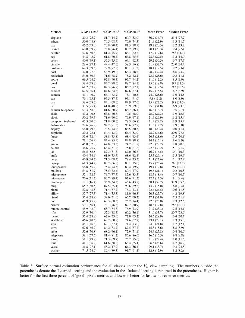
Normal Estimation. We show the performance plots fornormal estimation for all classes under the view samplingVn and Vd in Figure 3 and Figure 4 respectively. The per-formance under various metrics under the view sampling Vnand Vd are reported in Table 3 and Table 4 respectively.

11

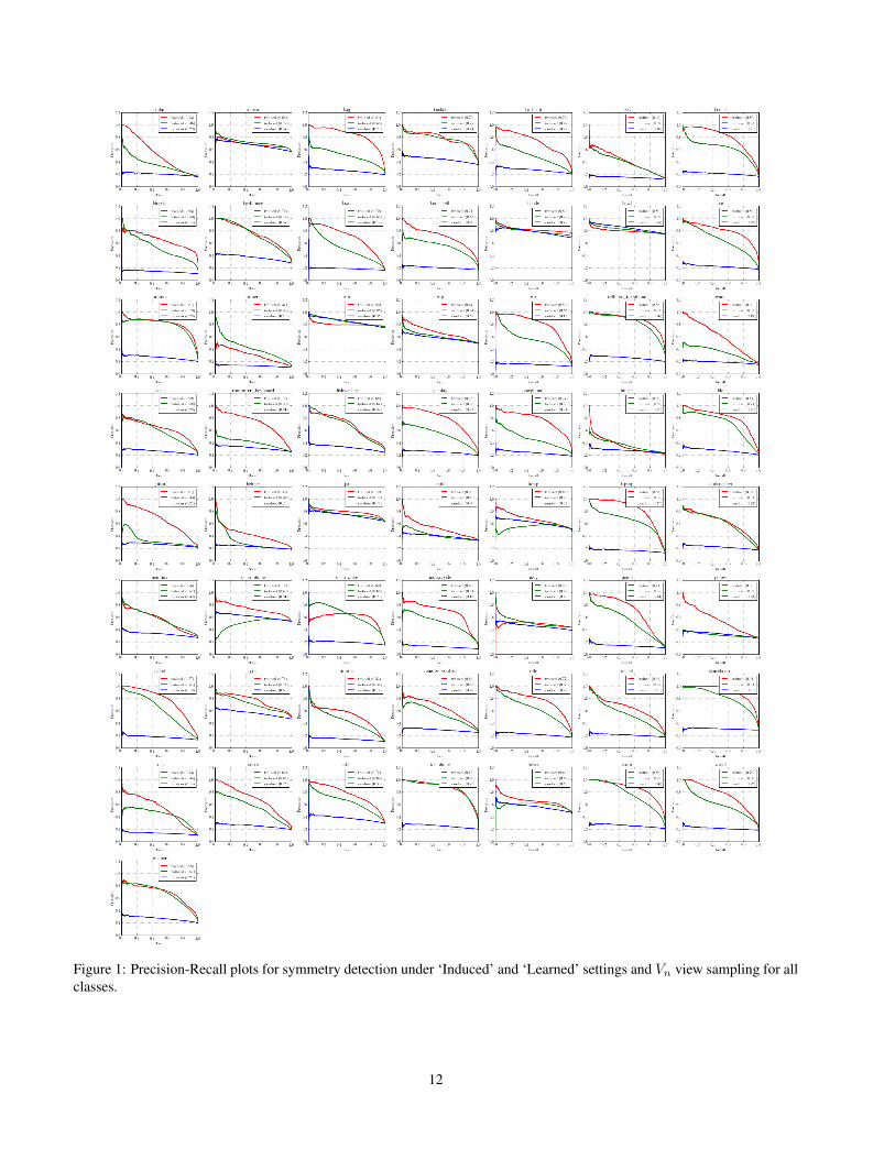
Figure 1: Precision-Recall plots for symmetry detection under ‘Induced’ and ‘Learned’ settings and Vn view sampling for allclasses.

12

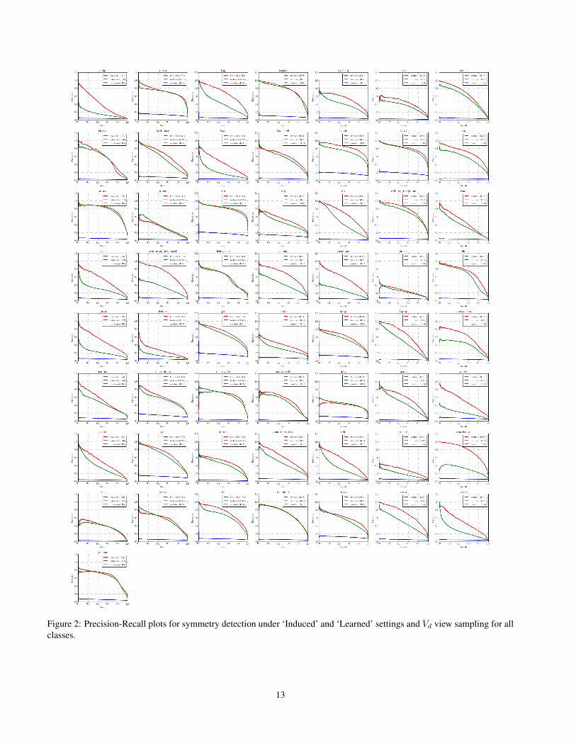
Figure 2: Precision-Recall plots for symmetry detection under ‘Induced’ and ‘Learned’ settings and Vd view sampling for allclasses.

13

View Setting VD VN

Learned Induced Random Learned Induced Random

airplane 0.41 0.16 0.04 0.53 0.36 0.20ashcan 0.73 0.70 0.14 0.69 0.72 0.67bag 0.68 0.42 0.05 0.84 0.50 0.26basket 0.78 0.76 0.10 0.79 0.77 0.44bathtub 0.54 0.40 0.05 0.73 0.49 0.27bed 0.44 0.36 0.03 0.42 0.39 0.15bench 0.66 0.57 0.05 0.80 0.63 0.21bicycle 0.57 0.56 0.03 0.65 0.53 0.14birdhouse 0.64 0.55 0.08 0.76 0.74 0.37boat 0.45 0.21 0.03 0.70 0.52 0.19bookshelf 0.61 0.56 0.04 0.71 0.55 0.20bottle 0.83 0.72 0.17 0.82 0.79 0.78bowl 0.81 0.78 0.18 0.80 0.82 0.85bus 0.71 0.57 0.04 0.80 0.65 0.22cabinet 0.78 0.77 0.05 0.81 0.79 0.26camera 0.32 0.36 0.03 0.31 0.42 0.13can 0.82 0.80 0.18 0.80 0.85 0.85cap 0.54 0.46 0.13 0.67 0.61 0.58car 0.66 0.46 0.03 0.80 0.55 0.15cellular telephone 0.77 0.71 0.05 0.88 0.83 0.26chair 0.48 0.39 0.04 0.60 0.35 0.19clock 0.53 0.29 0.05 0.62 0.58 0.26computer keyboard 0.70 0.34 0.06 0.72 0.40 0.31dishwasher 0.60 0.61 0.06 0.68 0.67 0.32display 0.66 0.42 0.05 0.78 0.53 0.25earphone 0.58 0.25 0.05 0.77 0.46 0.24faucet 0.25 0.24 0.06 0.36 0.36 0.27file 0.72 0.64 0.06 0.81 0.71 0.27guitar 0.52 0.22 0.05 0.67 0.33 0.27helmet 0.27 0.14 0.05 0.43 0.31 0.23jar 0.72 0.66 0.16 0.79 0.76 0.74knife 0.41 0.31 0.08 0.53 0.42 0.40lamp 0.61 0.54 0.12 0.68 0.55 0.62laptop 0.66 0.49 0.04 0.83 0.65 0.17loudspeaker 0.61 0.40 0.04 0.63 0.61 0.22mailbox 0.53 0.45 0.07 0.56 0.57 0.33microphone 0.60 0.54 0.15 0.74 0.50 0.61microwave 0.66 0.66 0.04 0.60 0.64 0.20motorcycle 0.54 0.48 0.03 0.69 0.51 0.12mug 0.41 0.44 0.11 0.49 0.52 0.46piano 0.58 0.46 0.03 0.71 0.55 0.14pillow 0.52 0.22 0.08 0.55 0.32 0.33pistol 0.48 0.36 0.04 0.77 0.61 0.18pot 0.70 0.65 0.12 0.76 0.71 0.56printer 0.49 0.42 0.03 0.53 0.44 0.14remote control 0.60 0.46 0.06 0.65 0.55 0.29rifle 0.54 0.34 0.05 0.77 0.63 0.22rocket 0.29 0.19 0.05 0.65 0.55 0.21skateboard 0.78 0.31 0.06 0.91 0.81 0.31sofa 0.39 0.37 0.03 0.53 0.44 0.14stove 0.56 0.56 0.05 0.69 0.55 0.25table 0.73 0.63 0.07 0.77 0.64 0.38telephone 0.71 0.71 0.05 0.86 0.86 0.25tower 0.60 0.56 0.12 0.66 0.59 0.56train 0.70 0.48 0.05 0.86 0.77 0.26vessel 0.50 0.27 0.04 0.76 0.60 0.22washer 0.65 0.64 0.06 0.68 0.67 0.27

Table 2: Performance across classes for symmetry prediction under AP θs metric.

14

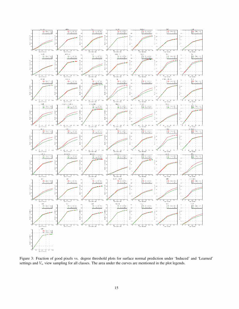
Figure 3: Fraction of good pixels vs. degree threshold plots for surface normal prediction under ‘Induced’ and ‘Learned’settings and Vn view sampling for all classes. The area under the curves are mentioned in the plot legends.

15

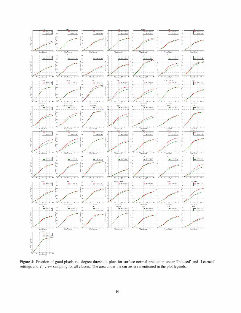
Figure 4: Fraction of good pixels vs. degree threshold plots for surface normal prediction under ‘Induced’ and ‘Learned’settings and Vd view sampling for all classes. The area under the curves are mentioned in the plot legends.

16

Metrics %GP 11.25◦ %GP 22.5◦ %GP 30.0◦ Mean Error Median Error

airplane 29.3 (25.2) 51.7 (44.2) 60.7 (53.0) 30.9 (34.7) 21.4 (27.2)ashcan 50.0 (48.8) 70.5 (68.7) 76.0 (74.3) 21.9 (22.9) 11.3 (11.5)bag 46.2 (43.0) 73.8 (70.4) 81.5 (78.9) 19.2 (20.5) 12.2 (13.2)basket 60.0 (59.7) 76.8 (76.4) 80.2 (79.8) 20.1 (20.3) 9.4 (9.5)bathtub 57.6 (50.8) 81.2 (75.7) 86.1 (82.2) 17.2 (19.6) 9.8 (11.1)bed 44.8 (43.2) 61.8 (60.4) 66.8 (65.6) 28.6 (29.5) 13.2 (14.0)bench 40.0 (39.1) 57.3 (55.6) 64.1 (62.3) 29.2 (30.3) 16.7 (17.7)bicycle 28.6 (27.1) 49.4 (47.6) 58.3 (56.8) 31.9 (32.7) 23.0 (24.4)birdhouse 62.3 (59.6) 79.9 (77.8) 83.1 (81.2) 18.4 (19.5) 9.2 (9.6)boat 32.0 (27.6) 56.9 (49.0) 66.3 (58.2) 28.2 (32.4) 18.6 (23.2)bookshelf 54.0 (50.6) 71.6 (68.2) 75.2 (72.2) 23.7 (25.6) 10.3 (11.1)bottle 69.5 (64.2) 92.8 (90.3) 95.7 (94.2) 11.0 (12.2) 8.5 (9.0)bowl 58.4 (48.8) 84.7 (78.5) 88.7 (84.1) 15.5 (18.8) 9.9 (11.5)bus 61.2 (53.2) 82.3 (76.9) 86.7 (82.1) 16.3 (19.5) 9.3 (10.5)cabinet 67.5 (66.1) 84.6 (84.3) 87.6 (87.4) 15.2 (15.5) 8.7 (8.9)camera 43.1 (40.9) 66.1 (63.2) 73.1 (70.3) 24.0 (25.6) 13.6 (14.5)can 76.1 (65.1) 95.5 (87.5) 97.1 (91.0) 9.8 (13.2) 8.0 (8.9)cap 58.6 (38.3) 84.1 (68.6) 87.9 (77.6) 15.9 (22.2) 9.8 (14.5)car 33.5 (25.4) 61.0 (48.8) 70.9 (59.0) 25.3 (31.8) 16.9 (23.3)cellular telephone 59.3 (58.6) 81.6 (80.9) 86.7 (86.1) 16.3 (16.7) 9.5 (9.7)chair 43.2 (40.5) 63.8 (60.8) 70.5 (68.0) 25.9 (27.3) 13.9 (15.3)clock 50.2 (39.3) 71.6 (60.0) 76.9 (67.1) 21.6 (26.9) 11.2 (15.4)computer keyboard 47.3 (40.0) 71.8 (60.6) 78.3 (66.8) 21.9 (29.2) 11.9 (15.4)dishwasher 79.6 (76.9) 92.2 (91.3) 93.6 (92.9) 11.6 (12.2) 7.9 (8.0)display 56.0 (49.6) 78.5 (74.2) 83.5 (80.3) 18.0 (20.4) 10.0 (11.4)earphone 29.2 (23.1) 54.4 (43.0) 64.4 (53.0) 28.9 (34.6) 20.0 (27.6)faucet 35.6 (32.4) 58.8 (53.8) 68.4 (63.6) 26.3 (28.6) 17.5 (20.1)file 71.1 (66.9) 87.4 (85.9) 89.8 (88.8) 14.2 (15.1) 8.6 (8.9)guitar 45.0 (32.8) 67.8 (53.3) 74.7 (61.8) 22.9 (29.7) 12.8 (20.3)helmet 36.6 (25.7) 66.4 (51.2) 75.8 (61.6) 22.6 (30.2) 15.1 (21.7)jar 56.5 (55.5) 82.3 (81.8) 87.0 (86.7) 16.2 (16.5) 10.1 (10.3)knife 40.4 (34.6) 61.0 (53.7) 68.6 (62.4) 25.5 (29.1) 15.5 (19.9)lamp 46.9 (44.7) 71.5 (68.3) 78.4 (75.5) 21.1 (22.6) 12.1 (12.9)laptop 61.3 (44.7) 83.7 (66.9) 88.1 (75.0) 15.7 (23.4) 9.6 (12.7)loudspeaker 56.8 (55.2) 75.4 (74.5) 80.4 (79.9) 19.4 (19.8) 9.9 (10.1)mailbox 54.8 (51.7) 75.5 (72.4) 80.4 (77.9) 19.6 (21.1) 10.2 (10.8)microphone 52.1 (52.5) 76.7 (77.7) 82.6 (83.5) 18.7 (18.4) 10.7 (10.7)microwave 76.6 (71.7) 90.7 (89.4) 92.6 (91.5) 12.3 (13.3) 8.1 (8.4)motorcycle 18.1 (16.4) 36.9 (34.2) 46.6 (43.8) 38.1 (39.7) 32.9 (35.5)mug 65.7 (60.5) 87.5 (85.1) 90.6 (89.2) 13.9 (15.0) 8.8 (9.4)piano 52.8 (48.8) 71.4 (67.7) 76.3 (73.1) 22.4 (24.5) 10.6 (11.5)pillow 37.7 (27.3) 71.4 (55.3) 81.0 (66.3) 20.3 (27.7) 14.2 (19.8)pistol 35.4 (28.8) 58.0 (51.0) 66.7 (60.2) 27.1 (31.0) 17.5 (21.9)pot 45.9 (45.2) 69.3 (68.5) 75.2 (74.4) 22.6 (23.0) 12.3 (12.5)printer 59.1 (56.1) 78.1 (76.3) 82.7 (80.9) 18.6 (19.8) 9.6 (10.1)remote control 45.9 (42.0) 68.7 (64.8) 76.9 (73.9) 21.7 (23.3) 12.5 (14.1)rifle 32.9 (30.4) 52.3 (48.5) 60.2 (56.1) 31.0 (33.7) 20.7 (23.9)rocket 35.4 (28.9) 62.6 (53.0) 72.0 (63.2) 24.5 (28.9) 16.4 (20.7)skateboard 46.6 (40.6) 68.2 (60.9) 74.6 (67.7) 23.4 (28.1) 12.3 (15.3)sofa 48.1 (46.8) 69.1 (67.4) 74.4 (73.0) 24.0 (24.8) 11.7 (12.1)stove 67.6 (66.2) 84.2 (83.7) 87.5 (87.2) 15.3 (15.6) 8.8 (8.9)table 52.6 (50.8) 68.2 (66.1) 72.9 (71.1) 24.6 (25.8) 10.4 (10.9)telephone 58.1 (57.6) 81.4 (81.2) 86.6 (86.6) 16.5 (16.5) 9.8 (9.8)tower 51.1 (49.2) 71.3 (69.7) 76.7 (75.6) 21.8 (22.4) 11.0 (11.5)train 41.1 (36.9) 61.6 (58.0) 68.4 (65.4) 26.5 (28.6) 14.7 (16.9)vessel 31.8 (27.1) 55.2 (47.2) 64.3 (56.1) 29.1 (33.7) 19.3 (24.8)washer 74.5 (74.9) 89.4 (89.3) 91.7 (91.4) 12.8 (12.9) 8.2 (8.2)

Table 3: Surface normal estimation performance for all classes under the Vn view sampling. The numbers outside theparenthesis denote the ‘Learned’ setting and the evaluation in the ‘Induced’ setting is reported in the parenthesis. Higher isbetter for the first three percent of ‘good’ pixels metrics and lower is better for last two three error metrics.

17

Metrics %GP 11.25◦ %GP 22.5◦ %GP 30.0◦ Mean Error Median Error

airplane 23.2 (20.0) 46.4 (38.8) 56.9 (47.6) 32.7 (37.7) 24.9 (32.3)ashcan 42.0 (42.3) 67.7 (67.1) 74.6 (73.8) 23.2 (23.6) 13.3 (13.3)bag 35.6 (34.0) 62.6 (59.1) 71.7 (68.1) 24.9 (26.9) 16.1 (17.2)basket 42.9 (42.9) 67.6 (65.7) 73.5 (71.3) 24.8 (26.0) 13.0 (13.2)bathtub 39.8 (32.8) 66.6 (59.1) 73.8 (67.3) 24.6 (28.6) 14.1 (17.4)bed 36.5 (34.0) 59.3 (56.9) 65.9 (63.8) 29.0 (30.5) 16.1 (17.6)bench 33.3 (32.4) 56.4 (54.3) 64.0 (61.9) 29.4 (30.7) 18.1 (19.2)bicycle 26.5 (25.6) 48.5 (47.8) 58.2 (57.9) 32.0 (32.2) 23.6 (24.1)birdhouse 44.4 (42.1) 71.4 (68.5) 78.0 (75.8) 22.2 (23.4) 12.6 (13.3)boat 25.7 (22.8) 49.2 (43.7) 58.5 (52.4) 32.6 (35.9) 23.1 (27.7)bookshelf 40.0 (36.7) 62.7 (59.7) 68.4 (65.6) 28.1 (30.0) 14.3 (15.9)bottle 57.6 (52.0) 88.1 (84.3) 93.0 (90.5) 13.4 (15.0) 10.0 (10.9)bowl 42.1 (30.9) 69.4 (55.0) 76.4 (63.6) 22.6 (29.5) 13.2 (19.0)bus 53.0 (46.4) 79.5 (74.5) 84.4 (80.4) 18.2 (21.1) 10.7 (12.0)cabinet 55.7 (56.3) 79.5 (79.7) 84.1 (84.1) 18.2 (18.2) 10.3 (10.2)camera 35.4 (34.9) 61.5 (59.6) 69.7 (67.6) 26.4 (27.7) 16.1 (16.7)can 64.8 (53.9) 90.6 (81.7) 93.6 (86.6) 12.6 (16.9) 9.1 (10.6)cap 49.5 (34.1) 79.0 (62.7) 83.9 (70.9) 18.9 (26.3) 11.3 (16.0)car 33.7 (25.7) 63.1 (51.1) 72.6 (61.2) 24.4 (30.7) 16.2 (21.8)cellular telephone 50.8 (50.3) 78.6 (78.1) 84.8 (84.2) 17.8 (18.1) 11.1 (11.2)chair 35.1 (33.1) 60.7 (57.7) 68.3 (65.4) 27.6 (29.2) 16.4 (17.6)clock 41.7 (33.5) 67.3 (57.9) 73.9 (64.9) 24.2 (29.6) 13.5 (17.4)computer keyboard 39.6 (31.5) 71.1 (59.8) 80.0 (69.2) 20.5 (26.7) 13.8 (17.5)dishwasher 66.9 (64.0) 89.2 (88.2) 91.9 (91.1) 13.4 (14.2) 9.0 (9.3)display 38.6 (29.3) 67.1 (52.8) 75.1 (60.7) 23.3 (31.5) 14.3 (20.4)earphone 28.1 (22.4) 53.1 (43.8) 62.8 (53.7) 30.1 (35.0) 20.6 (26.9)faucet 31.3 (29.5) 58.2 (55.7) 68.2 (65.7) 26.8 (28.3) 18.2 (19.3)file 59.9 (55.5) 83.1 (81.0) 86.4 (84.9) 16.8 (18.1) 9.7 (10.3)guitar 38.2 (27.6) 64.6 (48.6) 72.4 (56.6) 24.4 (33.5) 15.0 (23.7)helmet 36.3 (24.2) 68.6 (50.6) 78.4 (61.3) 21.5 (30.7) 14.9 (22.2)jar 43.0 (42.7) 71.0 (70.7) 78.0 (77.7) 21.6 (21.7) 12.9 (13.0)knife 32.9 (28.4) 56.2 (49.8) 65.3 (58.7) 28.2 (31.6) 18.6 (22.7)lamp 38.3 (36.5) 65.9 (62.6) 73.6 (70.7) 24.1 (25.6) 14.6 (15.5)laptop 46.2 (31.8) 75.9 (56.3) 82.0 (63.4) 20.1 (30.5) 12.1 (18.4)loudspeaker 49.7 (47.0) 73.6 (71.9) 79.0 (77.8) 20.9 (22.0) 11.3 (12.0)mailbox 42.4 (39.4) 68.3 (66.0) 76.0 (74.2) 22.5 (23.7) 13.3 (14.3)microphone 44.6 (41.3) 74.2 (70.4) 81.4 (78.1) 20.1 (22.0) 12.5 (13.5)microwave 65.4 (59.4) 87.9 (84.6) 90.8 (88.2) 14.2 (16.3) 9.0 (9.8)motorcycle 17.9 (16.9) 37.7 (35.8) 48.0 (46.1) 37.4 (38.4) 31.7 (33.3)mug 54.3 (49.7) 80.8 (78.5) 84.9 (83.5) 18.1 (19.2) 10.5 (11.3)piano 40.2 (35.7) 65.9 (60.9) 72.8 (68.2) 25.2 (27.9) 14.0 (16.1)pillow 33.4 (23.4) 66.7 (50.0) 77.3 (60.7) 22.3 (31.1) 15.8 (22.5)pistol 30.9 (27.2) 57.9 (53.3) 67.7 (63.7) 27.1 (29.5) 18.3 (20.6)pot 35.5 (33.8) 59.4 (58.2) 66.7 (65.7) 28.2 (28.8) 16.5 (17.3)printer 46.0 (42.1) 72.1 (68.5) 77.8 (74.5) 22.2 (24.4) 12.2 (13.2)remote control 38.0 (33.3) 65.3 (60.2) 73.8 (69.7) 23.9 (26.1) 15.0 (17.3)rifle 28.5 (27.1) 53.5 (51.3) 63.3 (61.0) 29.5 (30.6) 20.3 (21.7)rocket 28.7 (26.6) 54.7 (50.8) 64.7 (60.4) 28.6 (31.0) 19.8 (22.0)skateboard 45.8 (28.7) 75.9 (54.0) 82.3 (62.1) 19.9 (31.0) 12.1 (20.0)sofa 37.6 (36.5) 62.2 (60.0) 68.7 (66.3) 27.7 (29.2) 15.0 (15.8)stove 53.5 (51.4) 78.7 (77.4) 83.9 (82.7) 18.3 (19.2) 10.6 (11.0)table 53.2 (46.4) 76.7 (72.0) 81.1 (77.1) 19.9 (22.8) 10.6 (12.1)telephone 50.6 (50.5) 78.7 (78.9) 85.0 (85.4) 17.8 (17.7) 11.1 (11.1)tower 39.8 (39.2) 65.8 (63.9) 73.0 (71.2) 24.5 (25.3) 14.1 (14.5)train 34.5 (31.2) 60.1 (56.4) 68.3 (65.0) 27.2 (29.1) 16.6 (18.5)vessel 26.4 (23.7) 50.0 (45.1) 59.0 (53.7) 32.3 (35.3) 22.5 (26.6)washer 63.4 (65.0) 86.3 (87.0) 89.7 (90.2) 14.9 (14.5) 9.3 (9.1)

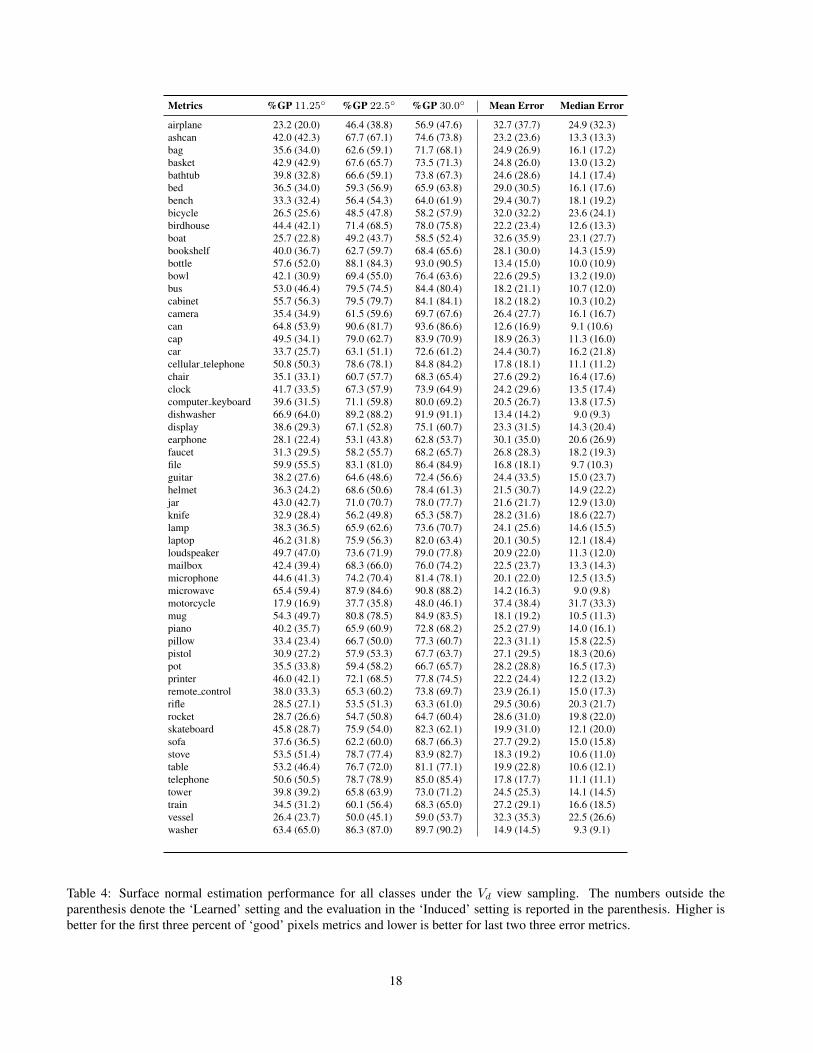
Table 4: Surface normal estimation performance for all classes under the Vd view sampling. The numbers outside theparenthesis denote the ‘Learned’ setting and the evaluation in the ‘Induced’ setting is reported in the parenthesis. Higher isbetter for the first three percent of ‘good’ pixels metrics and lower is better for last two three error metrics.

18