A Measure of Shape Dissimilarity for 3D Curves · Keywords: Shape-of-curve dissimilarity, 3D discrete curves, chain coding, measure of shape dissimilarity, 3D curve representation

Int. J. Contemp. Math. Sciences, Vol. 1, 2006, no. 15, 727 - 751

A Measure of Shape Dissimilarity

for 3D Curves

Ernesto Bribiesca1

Department of Computer ScienceInstituto de Investigaciones en Matematicas Aplicadas y en Sistemas

Universidad Nacional Autonoma de MexicoApdo. 20-726, Mexico, D.F., 01000. Fax: (5255)5622-3620

[email protected]

Wendy Aguilar

Department of Computer ScienceInstituto de Investigaciones en Matematicas Aplicadas y en Sistemas

Universidad Nacional Autonoma de MexicoApdo. 20-726, Mexico, D.F., 01000. Fax: (5255)5622-3620

[email protected]

Abstract

We present a quantitative approach to the measurement of shapedissimilarity between two 3D (three-dimensional) curves. Any 3D con-tinuous curve can be digitalized and represented as a 3D discrete curve.Thus, a 3D discrete curve is composed of constant orthogonal straight-line segments. In order to represent 3D discrete curves, we use theorthogonal direction change chain code. The chain elements representthe orthogonal direction changes of the contiguous straight-line seg-ments of the discrete curve. This chain code only considers relativedirection changes, which allows us to have a curve descriptor invari-ant under translation and rotation. Also, this curve descriptor may bestarting point normalized and mirroring curves may be obtained withease. Thus, using the above-mentioned chain code it is possible to havea unique 3D-curve descriptor.

To find out how close in shape two 3D curves are, a measure of shape-of-curve dissimilarity between them is introduced; analogous curves willhave a low measure of shape dissimilarity, while different curves willhave a high measure of shape dissimilarity. When this measure of shapedissimilarity is normalized, its values vary continuously from 0 to 1. If

1Author to whom correspondence should be addressed

728 E. Bribiesca and W. Aguilar

two curves are identical, the value of the measure of shape dissimilar-ity is equal to 0. The computation of this measure for two curves isbased on the analysis of their common and different subcurves repre-sented by their chain elements. Finally, we present some results of thecomputation of the proposed measure for 15 curves.

Mathematics Subject Classification: 65D17

Keywords: Shape-of-curve dissimilarity, 3D discrete curves, chain coding,measure of shape dissimilarity, 3D curve representation

1 Introduction

The study of the representation and comparison of 3D curves is an importanttopic in different fields. This paper gives a procedure to measure the resem-blance between any two 3D curves. With the help of procedures like this, aquantitative study of shape-of-curve dissimilarity may be possible. 3D curvesare represented by means of chain coding. Chain-code methods are widelyused because they preserve information and allow considerable data reduc-tion. Chain codes are the standard input format for numerous shape analysisalgorithms. Several shape features may be computed directly from the chain-code representation [8]. The first approach for representing 3D digital curvesusing chain code was introduced by Freeman in 1974 [7]. A canonical shapedescription for 3D stick bodies has been defined by Guzman [10]. In the con-tent of this work, we use the orthogonal direction change chain code [4] forrepresenting 3D curves. The main characteristics of this chain code are thefollowing: (1) it is invariant under translation and rotation; (2) optionally, itmay be starting point normalized and mirroring curves may be obtained withease; (3) there are only five possible orthogonal direction changes for repre-senting any 3D curve, which produces a numerical string of finite length overa finite alphabet, which allows us to use grammatical techniques for 3D-curveanalysis. Thus, using the above-mentioned chain code it is possible to have aunique 3D-curve descriptor.

The Hausdorff distance plays an important role in curve resemblance. Bel-ogay et al. [3] propose a method for computing the Hausdorff distance betweencurves. As a measure for the resemblance of curves in arbitrary dimensionsAlt and Godau [1] consider the so-called Frechet-distance, which is compatiblewith parametrizations of the curves. Arkin et al. [2] present an efficientlycomputable metric for comparing polygonal shapes based on turning anglerepresentation.

Several authors have proposed different measures of shape dissimilarity for3D curves. Li [13] proposes a system for matching and pose estimation of 3D

A Measure of Shape Dissimilarity for 3D Curves 729

curves under similarity transformation composed of translation, rotation anduniform scaling. Lo and Don [15] describe two invariant representations for 3Dcurves. One represents 3D curves by complex waveforms. The other illustrates3D curves using 3D moment invariants of the data points on the curves.

Other methods are focused on 3D shape recognition, for instance: Jain andHoffman [12] define a similarity measure between the set of observed featuresand the set of evidence conditions for a given object in a database. Dickinsonet al. [6] present some techniques for recognition of 3D objects from a single 2Dimage. In such techniques, from an input image, a set of features or primitivesmay be extracted. Lohmann [16] considers a similarity measure based on thequotients of volumes of the studied 3D objects over well-known geometricalobjects. Holden et al. [11] have evaluated eight different similarity measuresapplied to 3D serial magnetic resonance images. Recently, Rodriguez et al.[17] presented a new approach to measuring the similarity between 3D curves,this approach allows the possibility of using strings.

We present a measure of shape dissimilarity for 3D curves. In order torepresent 3D curves, we use the orthogonal direction change chain code. Thus,using this chain code we obtain a unique curve descriptor represented by achain. The measure of shape dissimilarity considers that two curves are moresimilar when they have in common more subcurves (one-to-one matching),and when these subcurves have the same orientation and position inside theircurves. This paper is organized as follows. In Section 2 we summarize theorthogonal direction change chain code. In Section 3 we describe the proposedmeasure of shape dissimilarity. Section 4 gives some results. Finally, in Section5 we present some conclusions.

2 The orthogonal direction change chain code

The purpose of this section is to summarize, in part, the orthogonal directionchange chain code which was presented in [4]. The concepts of this chain codeare important for describing the proposed measure of dissimilarity. Any 3Dcontinuous curve can be digitalized and represented as a 3D discrete curve.Thus, a 3D discrete curve is composed of constant orthogonal straight-linesegments. The chain elements represent the orthogonal direction changes ofthe constant straight-line segments of the 3D discrete curve. A chain A is anordered sequence of elements, and is represented by A = a1a2 . . . an = {ai :1 ≤ i ≤ n}, where n indicates the number of chain elements. A chain elementai indicates the orthogonal direction changes of the contiguous straight-linesegments of the 3D discrete curve in that chain-element position. In the contextof this work, the length l of each straight-line segment of any 3D curve isconsidered equal to one.

Each element of the chain labels a vertex of the 3D curve and indicates the


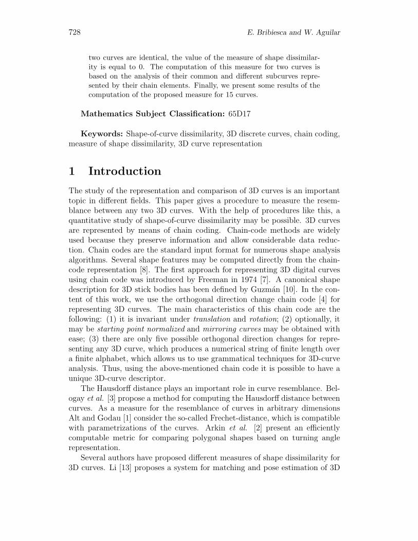
orthogonal direction changes of the polygonal path in such a vertex. There areonly five possible orthogonal direction changes for representing any 3D curve(figures 1(a)-(e) show these orthogonal direction changes):

1. The chain element “0” represents the direction change which goes straightthrough the contiguous straight-line segments following the direction ofthe last segment. This element is presented in Fig. 1(a).

2. The chain element “1” indicates a direction change to the right and isshown in Fig. 1(b)

3. The chain element “2” represents a direction change upward (stair-casefashion). This chain element is illustrated in Fig. 1(c).

4. The chain element “3” indicates a direction change to the left and isshown in Fig. 1(d).

5. The chain element “4” represents a direction change which is going backand is illustrated in Fig. 1(e).

Formally [5], if the consecutive sides of the reference angle have respectivedirections u and v (see Fig. 1(a)), and the side from the vertex to be labeledhas direction w (from here on by direction we understand a vector of length1), then the chain element is given by the following function,

chain element(u, v, w) =

⎧⎪⎪⎪⎪⎪⎨⎪⎪⎪⎪⎪⎩

0, if w = v;1, if w = u × v;2, if w = u;3, if w = −(u × v);4, if w = −u;

where × denotes the cross product.Fig. 1(f) illustrates an example of a continuous 3D curve. In order to

observe curves in a three-dimensional way, they are represented as ropes. Fig.1(g) shows the discrete version of the curve presented in (f) using only orthog-onal directions. The origin of this curve is considered at the lower side. Fig.1(h) shows the first element of the chain which corresponds to the element “3”.Notice that the first direction change (which is composed of two contiguousstraight-line segments) is used only for reference. Fig. 1(i) shows the nextelement obtained of the chain, which is based on the last direction changeof the first element; the second element corresponds to the element “3”, too.Fig. 1(j) show the next element obtained of the chain. Fig. 1(k) presentsall the chain elements of the 3D curve. Finally, Fig. 1(l) is the chain of theabove-mentioned curve, which is composed of seven chain elements.


Figure 1: The orthogonal direction change chain code: (a) the chain element“0”; (b) the chain element “1”; (c) the chain element “2”; (d) the chain element“3”; (e) the chain element “4”; (f) an example of a 3D curve; (g) the discreteversion of the curve shown in (f); (h) the first chain element of the chain;(i)-(k) next elements of the chain; (l) the chain of the above-mentioned curve.


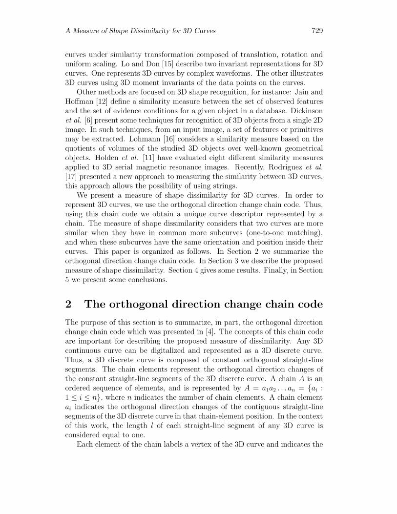
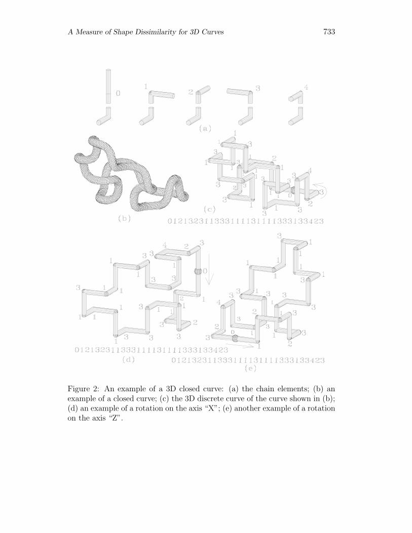
Fig. 2 illustrates an example of a 3D closed curve. Fig. 2(a) presentsthe chain elements, again. Fig. 2(b) shows an example of a closed continuouscurve. Fig. 2(c) illustrates the digitalized version of the curve shown in (b), itselements and its chain. The origin of this 3D discrete curve is represented bya sphere. Notice that when we are traveling a 3D curve in order to obtain itschain elements and find zero elements, we need to know what non-zero elementwas the last one in order to define the next element. In this manner orientationis not lost. Due to the fact that the orthogonal direction change chain codeonly considers relative direction changes, this chain code is invariant underrotation. Fig. 2(d) shows a rotation of the 3D discrete curve presented in(c) on the axis “X”. Fig. 2(e) illustrates another example of a rotation ofthe above-mentioned curve on the axis “Z”. Note that all chains are equal.Therefore, they are invariant under rotation. Using this notation its is possibleto obtain mirror images of curves with ease. The chain of the mirror imageof a curve is another chain (termed mirroring chain) whose elements “1” arereplaced by elements “3” and vice versa. This replacement does not dependon the orthogonal mirroring plane used, it is valid for all possible orthogonalplanes. The inverse of a chain of a curve is another chain formed of theelements of the first chain arranged in reverse order. Using the concept of theinverse of a chain, this notation may be starting point normalized by choosingthe starting point so that the resulting sequence of elements forms an integerof minimum magnitude. For a complete review of the orthogonal directionchange chain code and its properties, see ref. [4].

3 The measure of shape dissimilarity for curves

Since our goal is to give a measure of dissimilarity for 3D curves, we will startpresenting an intuitive definition of what similarity is. In ref. [14], Lin statesan intuitive definition of similarity as follows:

“Intuition 1: The similarity between A and B is related to their commonality.The more commonality they share, the more similar they are.

Intuition 2: The similarity between A and B is related to the differencesbetween them. The more differences they have, the less similar they are.

Intuition 3: The maximum similarity between A and B is reached when Aand B are identical, no matter how much commonality they share.”

A similarity measure is a function that associates a numeric value with (apair of) sequences (for example, two curves), with the idea that a higher valueindicates greater similarity, while a dissimilarity measure is the opposite, alower value indicates greater similarity.


Figure 2: An example of a 3D closed curve: (a) the chain elements; (b) anexample of a closed curve; (c) the 3D discrete curve of the curve shown in (b);(d) an example of a rotation on the axis “X”; (e) another example of a rotationon the axis “Z”.


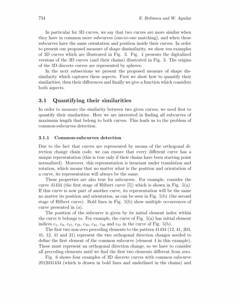
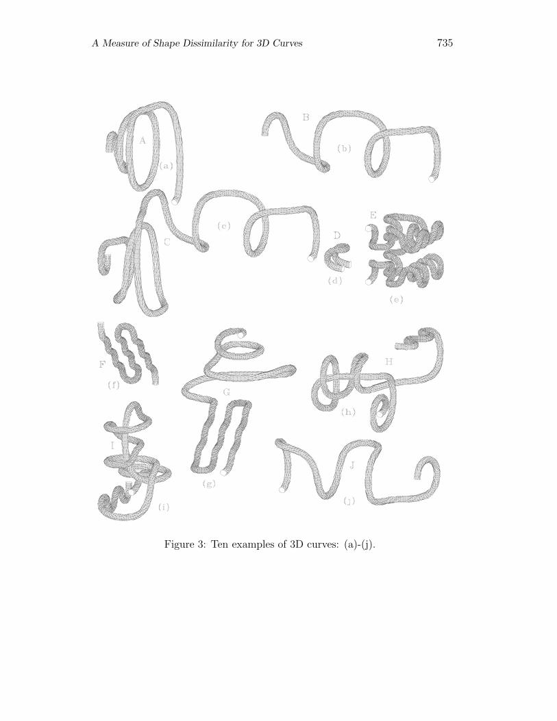
In particular for 3D curves, we say that two curves are more similar whenthey have in common more subcurves (one-to-one matching), and when thesesubcurves have the same orientation and position inside their curves. In orderto present our proposed measure of shape dissimilarity, we show ten examplesof 3D curves which are illustrated in Fig. 3. Fig. 4 presents the digitalizedversions of the 3D curves (and their chains) illustrated in Fig. 3. The originsof the 3D discrete curves are represented by spheres.

In the next subsections we present the proposed measure of shape dis-similarity which captures these aspects. First we show how to quantify theirsimilarities, then their differences and finally we give a function which considersboth aspects.

3.1 Quantifying their similarities

In order to measure the similarity between two given curves, we need first toquantify their similarities. Here we are interested in finding all subcurves ofmaximum length that belong to both curves. This leads us to the problem ofcommon-subcurves detection.

3.1.1 Common-subcurves detection

Due to the fact that curves are represented by means of the orthogonal di-rection change chain code, we can ensure that every different curve has aunique representation (this is true only if their chains have been starting pointnormalized). Moreover, this representation is invariant under translation androtation, which means that no matter what is the position and orientation ofa curve, its representation will always be the same.

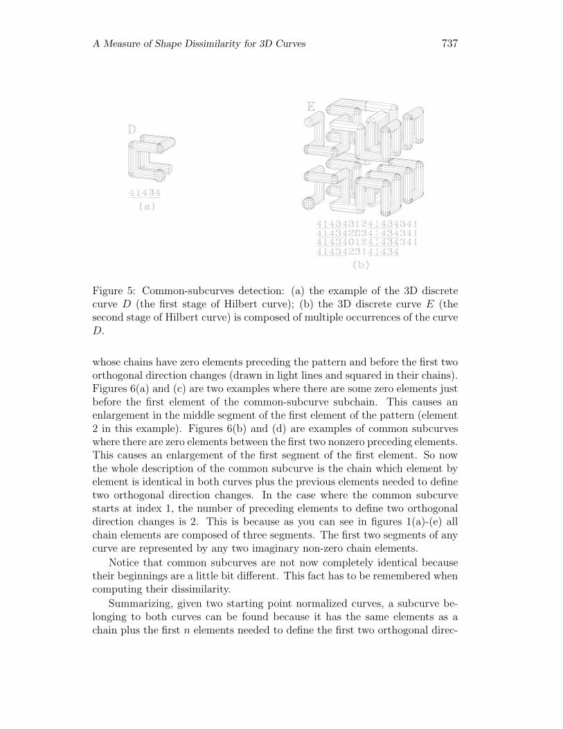
These properties are also true for subcurves. For example, consider thecurve 41434 (the first stage of Hilbert curve [5]) which is shown in Fig. 5(a).If this curve is now part of another curve, its representation will be the sameno matter its position and orientation, as can be seen in Fig. 5(b) (the secondstage of Hilbert curve). Bold lines in Fig. 5(b) show multiple occurrences ofcurve presented in (a).

The position of the subcurve is given by its initial element index withinthe curve it belongs to. For example, the curve of Fig. 5(a) has initial elementindices e1, e9, e17, e25, e33, e41, e49 and e57 in the curve of Fig. 5(b).

The first two non-zero preceding elements to the pattern 41434 (12, 41, 203,41, 12, 41 and 31) represent the two orthogonal direction changes needed todefine the first element of the common subcurve (element 4 in this example).These must represent an orthogonal direction change, so we have to considerall preceding elements until we find the first two elements different from zero.

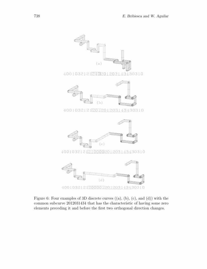
Fig. 6 shows four examples of 3D discrete curves with common subcurve2012031434 (which is drawn in bold lines and underlined in the chains) and


Figure 3: Ten examples of 3D curves: (a)-(j).


Figure 4: The digitalized versions of the ten 3D curves (and their chains)illustrated in Fig. 3, respectively: (a)-(j).


Figure 5: Common-subcurves detection: (a) the example of the 3D discretecurve D (the first stage of Hilbert curve); (b) the 3D discrete curve E (thesecond stage of Hilbert curve) is composed of multiple occurrences of the curveD.

whose chains have zero elements preceding the pattern and before the first twoorthogonal direction changes (drawn in light lines and squared in their chains).Figures 6(a) and (c) are two examples where there are some zero elements justbefore the first element of the common-subcurve subchain. This causes anenlargement in the middle segment of the first element of the pattern (element2 in this example). Figures 6(b) and (d) are examples of common subcurveswhere there are zero elements between the first two nonzero preceding elements.This causes an enlargement of the first segment of the first element. So nowthe whole description of the common subcurve is the chain which element byelement is identical in both curves plus the previous elements needed to definetwo orthogonal direction changes. In the case where the common subcurvestarts at index 1, the number of preceding elements to define two orthogonaldirection changes is 2. This is because as you can see in figures 1(a)-(e) allchain elements are composed of three segments. The first two segments of anycurve are represented by any two imaginary non-zero chain elements.

Notice that common subcurves are not now completely identical becausetheir beginnings are a little bit different. This fact has to be remembered whencomputing their dissimilarity.

Summarizing, given two starting point normalized curves, a subcurve be-longing to both curves can be found because it has the same elements as achain plus the first n elements needed to define the first two orthogonal direc-


Figure 6: Four examples of 3D discrete curves ((a), (b), (c), and (d)) with thecommon subcurve 2012031434 that has the characteristic of having some zeroelements preceding it and before the first two orthogonal direction changes.


tion changes. So, the problem of common-subcurves detection is reduced tothe string-matching problem, in particular, to the problem of finding all thelongest common substrings of two strings. Let A be the first string of lengthm, and B the second string of length n. A bruteforce matching algorithm canbe used, which consist of starting at the first element of each string and thenshifting A (with wrap-around in the case of closed curves) and keeping allcommon substrings of maximum length found during this process. Then, dothe same for every element of B. This can be computed in O(m×n). However,better algorithms that use suffix trees can be found in [9].

3.1.2 Dissimilarity measure for common subcurves

Once all common subcurves of maximum length have been detected, it could bepossible that two or more common subcurves have overlaps. For this reasonwe need to find a one-to-one matching between them. For this purpose wepropose a dissimilarity measure for common subcurves. This measure givesus a parameter to choose the best matching in case there are overlaps. Thecharacteristics used to evaluate their dissimilarity are: orientation, size andposition within their curves. One extra characteristic is if their beginningsare identical as explained in the previous subsection. The size is given bythe length of the subchain, the position by its starting element index and itsbeginning by the number of elements preceding the pattern needed to definetwo orthogonal direction changes for the first element of the common subcurve.The orientation of the curve can be calculated as follows.

3.1.2.1 Accumulated direction

The accumulated direction is the final orientation of a curve (or subcurve)after it has been affected by all its preceding chain elements. In other words,it is composed of two direction vectors which are the reference to define thenext element of the curve.

For the first chain element, these two direction vectors are given arbitrarily,the only restriction is that they have to be orthogonal to each other. Forexample, u’= (0, 1, 0) and d’= (−1, 0, 0). We also need to append at thebeginning of the chain two (non-zero) imaginary reference chain elements tobe used as a reference for the first element of the chain.

The new direction vectors u and d, are calculated in terms of the cur-rent direction vectors u’ and d’ and depending on the current chain element,according to the next rule.

Element 0 u = u’ d = d’Element 1 u = d’ d = u’ × d’Element 2 u = d’ d = u’


Element 3 u = d’ d = − (u’ × d’)Element 4 u = d’ d = −u’

Where u’ × d’ denotes the cross product for vectors. Thus, the accumulateddirection for a curve is given by the final vectors u and d resulting from applyingthis rule to all the elements of the curve.

Definition 1. Pseudo-metric of accumulated direction.Let A and B be two chains with accumulated directions (u,d) and (x,w) re-spectively. The pseudo-metric of accumulated direction is defined as follows.

Δ(A,B) ={

0 if u = x and d = w;1 otherwise.

(1)

It can be proved that the pseudo-metric of accumulated direction is a pseudo-metric, since it satisfies the properties of non-negativity, symmetry, identityand the triangle inequality. Notice that it does not satisfy the property ofuniqueness because there are different curves with the same accumulated di-rection. Curves of figures 4(a), (b), and (j) are examples of different curveswith the same accumulated direction.

3.1.2.2 Dissimilarity measure between two subchains of a partialcommon couple

Definition 2. Subchain.Let A = a1a2...am be a chain. A subchain S of A with initial index i is definedas:

S = aiai+1...an such that 1 ≤ i ≤ m and n ≤ m

Definition 3. Maximum common subchain.Let A = a1a2...am and B = b1b2...bn be two chains. A maximum commonsubchain S of A and B with initial indices q and r respectively, satisfy thefollowing conditions:

i) 1 ≤ L(S) ≤ min(m,n)ii) S is a subchain of A and B, with initial indices q and r respectively.iii) aq−1 �= br−1 and aq+L(S) �= br+L(S)

whereL(S) is the length of the subchain.

1 ≤ q ≤ m and 1 ≤ r ≤ n


Definition 4. Left maximization.Let A = a1a2...am and B = b1b2...bn be two chains. Let S be a subchain of Aand B, with initial index i in A and initial index j in B, such that:

A = a1a2...aiai+1...ai+L(S)−1...am where,ai = s1, ai+1 = s2, ..., ai+L(S)−1 = sL(S)

B = b1b2...bjbj+1...bj+L(S)−1...bn where,bj = s1, bj+1 = s2, ..., bj+L(S)−1 = sL(S)

The function lmax is defined as:lmax(A, B, S) = akak+1...aiai+1...ai+L(S)−1 = bk′ bk′+1...bjbj+1...bj+L(S)−1 =ulmax

where ulmax is a maximum subchain of A′ = a1a2...ai+L(S)−1 and B′ = b1b2...bj+L(S)−1.

Intuitively, lmax is a function that expands the subchain S to its left un-til S becomes a maximum subchain of A′ and B′. Index k is named ”leftmaximization index in A” and index k’ is named ”left maximization index inB”.

Definition 5. Partial Common Couple.Let A = a1a2...am and B = b1b2...bn be two chains. Let P ’ be a common sub-chain of A and B with initial indices i’1 and i’2 respectively, and L(P ’) = k’,for 1 ≤ k’≤ min(m,n).

P′= p

′1p

′2...p

′k′

Let P = lmax(A, B, P ’), with left maximization index in A i1 and left maxi-mization index in B i2.

P = p1p2...pk = ai1ai1+1 ...ai1+L(P )−1 = bi2bi2+1 ...bi2+L(P )−1

Let S be a subchain of A with initial index 1 and L(S) = i1 + L(P ) − 1.

S = a1a2...ai1ai1+1...ai1+L(P )−1 = a1a2...p1p2...pk

Let T be a subchain of B with initial index 1 and L(T ) = i2 + L(P ) − 1.

T = b1b2...bi2bi2+1...bi2+L(P )−1 = b1b2...p1p2...pk.

For convenience the couple (S,T) will be named partial common couple.


Given two chains, A and B, the minimum number of partial common cou-ples they could have is zero. This happens when A and B are completelydifferent, in other words, the two chains do not have any chain element incommon. While the maximum number of partial common couples they couldhave is given by the following expression:

(n0A × n0B) + (n1A × n1B) + (n2A × n2B) + (n3A × n3B) + (n4A × n4B)

where the notation n0A means “the number of zero elements in A”.

As an example, consider the chains D and G shown in Fig. 4. The maxi-mum number of partial common couples D and G could have is:

0 × 27 + 1 × 6 + 0 × 16 + 1 × 8 + 3 × 6 = 32

All their partial common couples (S, T ) are (P is shown in boldface):

1. (4143), 22222143)

2. (4143 , 2222214322222143)

3. (41434, 2222214)

4. (41434, 222221432222214)

5. (41434, 222221432222214322222100200000400003100003000400031003 004031034)

6. (41 , 2222214322222143222221)

7. (4 , 2222214)

8. (4 , 222221432222214)

9. (414 , 22222143222221432222210020000040000310000300040003100300 4031034)

10. (41 , 222221432222214322222100200000400003100003000400031003004 031)

11. (4 , 222221432222214322222100200000400003100003000400031003004 031034)

12. (4143 , 22222143222221432222210020000040000310000300040003100 3)

13. (4143 , 222221432222214322222100200000400003100003000400031003 00403)

14. (41 , 222221432222214322222100200000400003100003000400031 )

15. (4143 , 22222143222221432222210020000040000310000 3)

16. (41434, 222221432222214322222100200000400003100003000400031003 004)

17. (414 , 22222143222221432222210020000040000310000300040003100300 4)

18. (41 , 222221432222214322222100200000400003 1)

19. (4 , 222221432222214322222100200000400003100003000400031003 004)

20. (4143 , 2222214322222143222221002000004000031000030004000 3)

21. (41434, 2222214322222143222221002000004)

22. (41434, 2222214322222143222221002000004000031000030004)


23. (414 , 2222214322222143222221002000004)

24. (414 , 2222214322222143222221002000004000031000030004 )

25. (4 , 2222214322222143222221002000004)

26. (4 , 2222214322222143222221002000004000031000030004 )

27. (4143 , 222221432222214322222100200000400003)

Definition 6. Dissimilarity measure for partial common couples.The dissimilarity for partial common couples is defined as:

d(S, T ) =

⎧⎪⎪⎪⎨⎪⎪⎪⎩

0, when S = T|L(S)−L(T )|

max(L(S),L(T ))−1+ (min(m,n) − L(P ))+

Δ(S, T ) + |neS − neT | , when S �= T(2)

where,

|L(S)−L(T )|max(L(S),L(T ))−1

measures the displacement of the two common subchainswithin their respective curves, in such a way that if the correspondence inposition is exact this term becomes zero. This term is normalized to the range[0-1].

(min(m,n) − L(P )) measures how large are the common subchains withrespect to the curve where they are contained.

Δ(S, T ) is the pseudo-metric of accumulated direction of S and T . In otherwords, this term measures whether the final orientation of the subcurves S andT is the same. If it is the same, then this term becomes zero.

|neS − neT | measures the number of preceding elements to P in S and Tneeded to define two orthogonal direction changes as explained in subsection3.1.1.

It can be proved that this dissimilarity measure for partial common cou-ples is a metric, since it satisfies the properties of non-negativity, symmetry,identity, uniqueness and the triangle inequality.

This measure becomes more intuitive when it is bounded to the range of[0, 1], where 0 means that the two subchains are identical and 1 that they arecompletely different. For this purpose, the bounded dissimilarity measure forpartial common couples, which is also a metric, is now defined.

Definition 7. Bounded dissimilarity measure for partial common couples.The bounded dissimilarity measure for partial common couples is given by:

d(s, t) =d(s, t)

m + n. (3)


3.1.3 Finding one-to-one matching

After all maximum common subcurves have been detected, it is possible tohave overlaps between them, in other words, it is posible that two or morecommon subcurves share some elements. Formally,

Definition 8. Partial common couples overlap.Two partial common couples (S, T ) and (S’, T ’) of A and B, with maximumcommon subchains

P = p1p2...pk = ai1ai1+1...ai1+k−1 = bi2bi2+1...bi2+k−1

Q = q1q2...qr = ai3ai3+1...ai3+r−1 = bi4bi4+1...bi4+r−1

respectively, with initial indices i1 in A and i2 in B for P , and initial indicesi3 in A and i4 in B for Q, do not have overlap if the subchains:

P ′ = p′1p′2...p

′k′ = ai′1ai′1+1...ai′1+k′−1 = bi′2bi′2+1...bi′2+k′−1

Q′ = q′1q′2...q

′r′ = ai′3ai′3+1...ai′3+r′−1 = bi′4bi′4+1...bi′4+r′−1

before left maximization, P = lmax(A, B, P ′) and Q = lmax(A, B, Q′), satisfy:

{i′1 − neS, ..., i′1 − 1, i′1, i′1 + 1, ..., i′1 + k′ − 1}⋂

{i′3 − neS′ , ..., i′3 − 1, i′3, i′3 + 1, ..., i′3 + r′ − 1} = ∅

{i′2 − neT , ..., i′2 − 1, i′2, i′2 + 1, ..., i′2 + k′ − 1}⋂

{i′4 − neT ′ , ..., i′4 − 1, i′4, i′4 + 1, ..., i′4 + r′ − 1} = ∅

where the number of elements needed to define two orthogonal direction changes,neS, neS′,neT , neT ′, are with respect to P ′ and Q′.

Let {(Sj′, Tj′)} be the set of all partial common couples of curves A andB. For example, the one shown in subsection 3.1.2.2. This set is first sortedaccording to their dissimilarity measure using Eq. (3). The computation of Eq.(3) is linear in the number of partial common couples of A and B. If two partialcommon couples in this set have overlap between them, then the one that hasa lower dissimilarity d is chosen. The eliminated partial common couples areinspected to find out if there are still parts of them that could be matchedwithout overlap, thus subchains P ′

j must satisfy the following conditions:

• they are maximum common subchains of A and B, or


• they are subchains of maximum common subchains of A and B that weredivided because they had overlap.

Finally, let {Sj , Tj} be the set of all partial common couples of A and B,with no overlap with other partial common couple in this set. The similaritiesbetween A and B are given by:

l∑j=1

d(Sj, Tj)

where

(Sj, Tj) is the j-th partial common couple found in A and B with no overlapwith other partial common couples chosen.

l is the total number of partial common couples found in A and B withoutoverlap.

3.2 Quantifying their differences

To quantify the differences between two given curves, the number of elementsleft without correspondence is computed. Formally, the differences betweenthe curves A and B is given by

m + n −⎛⎝ l∑

j=1

2L(P ′j) + neSj

+ neTj

⎞⎠ + 4

where

P ′j is the j-th subchain that corresponds to the j-th partial common couple,

before the left maximization.

neSj, neTj

are the number of elements in Sj and Tj needed to define andorthogonal direction change with respect to P ′

j .

m is the number of elements of curve A.

n is the number of elements of curve B.

3.3 Dissimilarity measure for 3D curves

Definition 9. Dissimilarity measure for 3D curves.Let A = a1a2...am and B = b1b2...bn be two chains. The dissimilarity of A andB is defined as:


D(A, B) =l∑

j=1

d(sj , tj) +

⎡⎣m + n −

⎛⎝ l∑

j=1

2L(P ′j) + neSj

+ neTj

⎞⎠ + 4

⎤⎦ (4)

Notice that the first term measures the similarities between A and B whilethe second term measures their differences.

It can be proved that this dissimilarity measure satisfy the properties ofnon-negativity, symmetry, identity and uniqueness. Notice that the propertyof triangle inequality is not satisfied, thus it is not a metric.

This measure of dissimilarity becomes more intuitive when it is boundedto the range of [0, 1].

Definition 10. Bounded dissimilarity measure for 3D curves.The bounded dissimilarity measure for 3D curves is defined as:

D(A, B) =D(A, B)

m + n + 4. (5)

4 Results

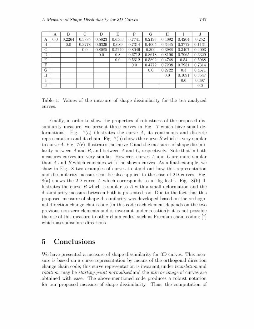
To illustrate the capabilities of the measure of shape dissimilarity proposedhere, we present the values of the measure for all 3D discrete curves shown inFig. 4. Thus, Table 1 summarizes the computations of the different measuresof shape dissimilarity for the ten analyzed curves. The values of these measuresare normalized and vary continuously from 0 to 1. These values were computedusing Eq. (5). When two curves are identical, the value of the measure of shapedissimilarity is equal to zero.

Analyzing the values of the measures of shape dissimilarity in Table 1, thetwo most similar curves of the ten studied above are the curves H and I (theirvalue of measure of shape dissimilarity is equal to 0.1091). The curves B andJ are also very similar their value is equal to 0.1131. An interesting examplecorresponds to the curves A and B, both have a value equal to 0.2264 whichindicates that they are very similar. Note that both curves look like spirals.Thus, in this case the value of the measure was not affected too much by theintercalated zero elements. On the other hand, the most dissimilar curves arethe following: curves D and G; D and H; C and D; and C and F, respectively.The values of the measure of shape dissimilarity are greater than 0.8.


A B C D E F G H I JA 0.0 0.2264 0.3885 0.5823 0.6563 0.7741 0.2193 0.4092 0.4204 0.252B 0.0 0.3278 0.6329 0.689 0.7314 0.4005 0.3445 0.3772 0.1131C 0.0 0.8085 0.5249 0.8046 0.309 0.3988 0.3407 0.4003D 0.0 0.8 0.6712 0.8618 0.8196 0.7965 0.6329E 0.0 0.5612 0.5892 0.4748 0.54 0.5968F 0.0 0.4772 0.7208 0.7951 0.7314G 0.0 0.2722 0.3 0.4571H 0.0 0.1091 0.3547I 0.0 0.397J 0.0

Table 1: Values of the measure of shape dissimilarity for the ten analyzedcurves.

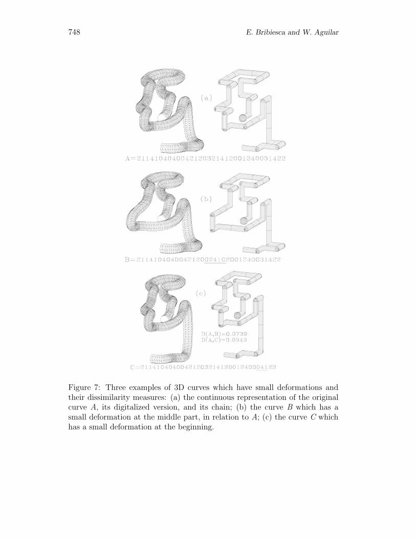
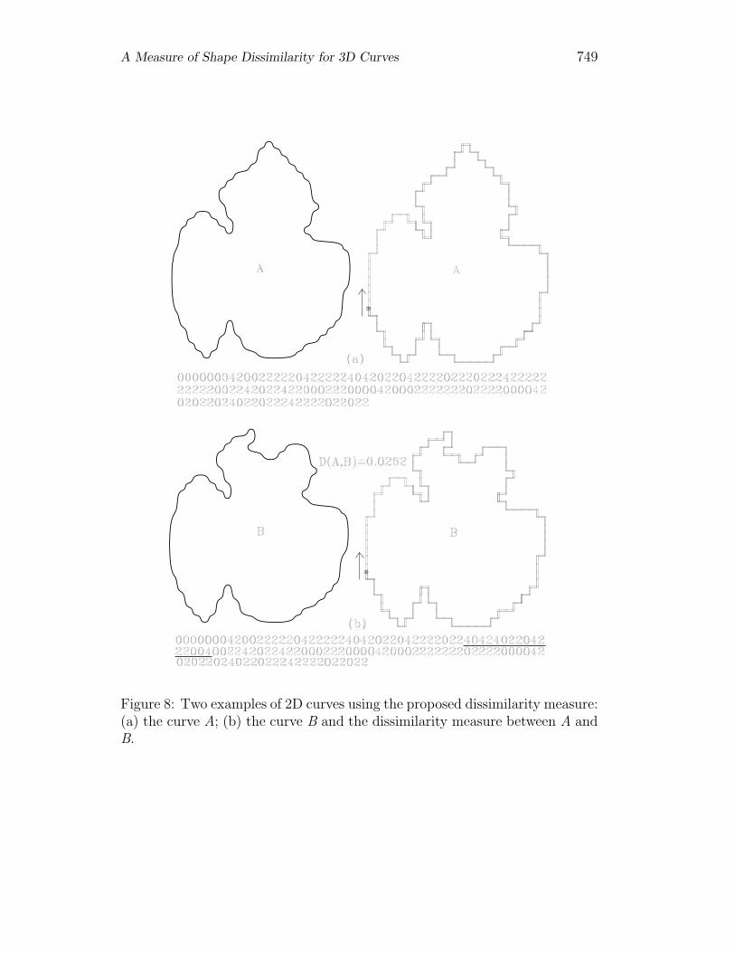
Finally, in order to show the properties of robustness of the proposed dis-similarity measure, we present three curves in Fig. 7 which have small de-formations. Fig. 7(a) illustrates the curve A, its continuous and discreterepresentation and its chain. Fig. 7(b) shows the curve B which is very similarto curve A. Fig. 7(c) illustrates the curve C and the measures of shape dissimi-larity between A and B, and between A and C, respectively. Note that in bothmeasures curves are very similar. However, curves A and C are more similarthan A and B which coincides with the shown curves. As a final example, weshow in Fig. 8 two examples of curves to stand out how this representationand dissimilarity measure can be also applied to the case of 2D curves. Fig.8(a) shows the 2D curve A which corresponds to a “fig leaf”. Fig. 8(b) il-lustrates the curve B which is similar to A with a small deformation and thedissimilarity measure between both is presented too. Due to the fact that thisproposed measure of shape dissimilarity was developed based on the orthogo-nal direction change chain code (in this code each element depends on the twoprevious non-zero elements and is invariant under rotation): it is not possiblethe use of this measure to other chain codes, such as Freeman chain coding [7]which uses absolute directions.

5 Conclusions

We have presented a measure of shape dissimilarity for 3D curves. This mea-sure is based on a curve representation by means of the orthogonal directionchange chain code; this curve representation is invariant under translation androtation, may be starting point normalized and the mirror image of curves areobtained with ease. The above-mentioned code produces a robust notationfor our proposed measure of shape dissimilarity. Thus, the computation of


Figure 7: Three examples of 3D curves which have small deformations andtheir dissimilarity measures: (a) the continuous representation of the originalcurve A, its digitalized version, and its chain; (b) the curve B which has asmall deformation at the middle part, in relation to A; (c) the curve C whichhas a small deformation at the beginning.


Figure 8: Two examples of 2D curves using the proposed dissimilarity measure:(a) the curve A; (b) the curve B and the dissimilarity measure between A andB.


this measure for two curves is based on the analysis of their common and dif-ferent subcurves represented by their chain elements. This analysis allows usto detect dissimilarity of shape for curves. Generally speaking, we proposedthat two curves are more similar when they have in common more subcurves,and when these subcurves have the same orientation and position inside theircurves. Finally, we presented some results of the computation of the proposedmeasure for 15 curves.

ACKNOWLEDGEMENT. This work was supported by IIMAS-UNAM.

References

[1] H. Alt, M. Godau, Computing the Frechet distance between 2 polygonalcurves, International Journal of Computational Geometry & Applications5 (1-2) (1995), 75-91.

[2] E. M. Arkin, L. P. Chew, D. P. Huttenlocher, K. Kedem, J. S. B. Mitchel,An efficiently computable metric for comparing polygonal shapes, IEEETransactions on Pattern Analysis and Machine Intelligence 13 (3) (1991),209-216.

[3] E. Belogay, C. Cabrelli, U. Molter, R. Shonkwiler, Calculating the Haus-dorff distance between curves, Information Processing Letters 64 (1997),17-22.

[4] E. Bribiesca, A chain code for representing 3D curves, Pattern Recognition33 (2000), 755-765.

[5] E. Bribiesca and C. Velarde, A formal language approach for a 3D curverepresentation, Computers & Mathematics with Applications 42 (2001),1571-1584.

[6] S. J. Dickinson, A. P. Pentland, A. Rosenfeld, From volumes to views:an approach to 3-D object recognition, CVGIP: Image Understanding 55(1992), 130-154.

[7] H. Freeman, Computer processing of line drawing images, ACM Comput-ing Surveys 6 (1974), 57-97.

[8] R. C. Gonzalez and R. E. Woods, Digital Image Processing, Second Edi-tion, Prentice Hall, Upper Saddle River, New Jersey 07458, 2002.

[9] D. Gusfield, Algorithms on Strings, Trees, and Sequences, CambridgeUniversity Press, Cambridge CB2 1RP, 1997.


[10] A. Guzman, Canonical shape description for 3-d stick bodies, MCC Tech-nical Report Number: ACA-254-87, Austin, TX. 78759 (1987).

[11] M. Holden, D. L. G. Hill, E. R. E. Denton, J. M. Jarosz, T. C. S. Cox, TRohlfing, J. Goodey, D. J. Hawkes, Voxels similarity measures for 3-D se-rial MR brain image registration, IEEE Transactions on Medical Imaging19 (2000), 94-102.

[12] A. K. Jain, R. Hoffman, Evidence-based recognition of 3-D objects, IEEETransactions on Pattern Analysis and Machine Intelligence 10 (1988),783-802.

[13] Stan Z. Li, Invariant representation, matching and pose estimation of 3Dspace curves under similarity transformations, Pattern Recognition 30 (3)(1997), 447-458.

[14] D. Lin, An Information-Theoretic Definition of Similarity. Proc. of theFifteenth International Conference on Machine Learning, Madison, Wis-consin, pp. 296-304 (1998).

[15] Chong-Huah Lo and Hon-Son Don, Invariant representation and matchingof space curves, Journal of Intelligent and Robotic Systems 28 (2000),125-149.

[16] G. Lohmann, Volumetric Image Analysis, Wiley & Sons and B. G. Teub-ner Publishers, New York, NY, 1998.

[17] W. Rodriguez, M. Last, A. Kandel, H. Bunke, 3-Dimensional curve simi-larity using string matching, Robotics and Autonomous Systems 49 (3-4)(2004) 165-172.

Received: May 19, 2006

Documents

A Measure of Shape Dissimilarity for 3D Curves · Keywords: Shape-of-curve dissimilarity, 3D discrete curves, chain coding, measure of shape dissimilarity, 3D curve representation