• Overview - different methods and applications • “Physics-based” model inversion methods • High spatial resolution imagery and Sentinel-2 • Bottom mapping • Satellite derived bathymetry (SDB)

• Sun-glint correction of high spatial resolution images • Model inversion methods and uncertainty propagation

Shallow Water Remote Sensing John Hedley, IOCCG Summer Class 2018

Objectives of shallow water remote sensing

• Bottom mapping - corals, seagrasses, macroalgae

• Water optical properties • Bathymetry (depth)

Applications • Spatial ecology (science) • MPA design (resource mapping) • Assessing ecosystem services - coastal protection and stabilisation - fisheries, local subsistence - blue carbon - tourism

Applications on coral reefs and similar environments

Hedley et al. 2016, Remote Sensing, 8, 118; doi:10.3390/rs8020118 Hedley et al. 2018, RSE Sentinel-2 special issue (in press, probably)

Need higher spatial resolution than typical ocean colour satellites

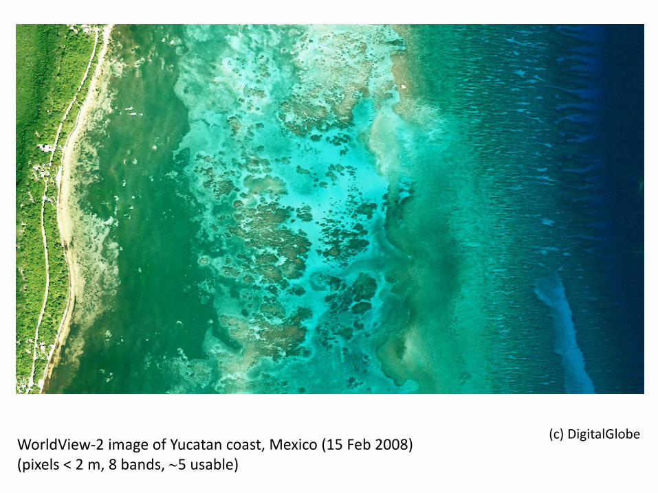
WorldView-2 image of Yucatan coast, Mexico (15 Feb 2008) (pixels < 2 m, 8 bands, ∼5 usable)

(c) DigitalGlobe

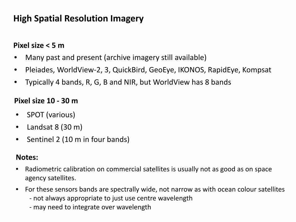
High Spatial Resolution Imagery

• Many past and present (archive imagery still available) • Pleiades, WorldView-2, 3, QuickBird, GeoEye, IKONOS, RapidEye, Kompsat • Typically 4 bands, R, G, B and NIR, but WorldView has 8 bands

Pixel size < 5 m

Pixel size 10 - 30 m

• SPOT (various) • Landsat 8 (30 m) • Sentinel 2 (10 m in four bands)

Notes: • Radiometric calibration on commercial satellites is usually not as good as on space

agency satellites. • For these sensors bands are spectrally wide, not narrow as with ocean colour satellites - not always appropriate to just use centre wavelength - may need to integrate over wavelength

WorldView-2 image of Yucatan coast, Mexico (15 Feb 2008) (pixels < 2 m, 8 bands, ∼5 usable)

(c) DigitalGlobe

Sentinel-2 image of Yucatan coast, Mexico (17 April 2018) (pixels 10 m, ∼5 usable bands)

ESA / Copernicus

Sentinel 2 - useful bands are at different resolutions

→ Interesting potential issues / artefacts

Methods for bottom mapping and/or bathymetry Many and very diverse − overlap with terrestrial methods Empirical, image based, requires training from in-situ data • Classification, depth invariant indices • Bathymetry by regression methods Physics based • Radiative transfer model inversion Hybrid • Object orientated techniques - classificaton combined with rules

which can take data from other remote sensing and physics based methods

• e.g. depth, wave energy (wind)

Stumpf et al. 2003

Lyzenga 1978 a0, a1, a2 from regression

m0, m1, from regression

Empirical image based methods (e.g. bathymetry) • Usually assume exponential attenuation of light with depth (i.e. constant Kd) • Requires training of points from imagery (deep water, known depths etc.) • Similar methods for water column correction, change detection, etc.

Benthic classification example, Lizard Island, GBR

Depth invarient indices

Classification

One method - depth invariant indices

• Works by identifying pixels that have similar spectral reflectances • Supervised or unsupervised • Need for water column correction

only need ratio of attenuation coefficients can extract from image using sand at different depths

Sun-glint : different types of glint dependent on spatial scale

High spatial resolution, pixels < 10 m → individual waves

Large images e.g. MERIS, pixels > 100 m → function of solar-view geometry and sea state

Eg. IKONOS, QuickBird, WorldView 2, Sentinel 2

Atmospheric contribution and surface glint

1) Direct Glint 2) Atmospheric Reflectance 3) Part We Want

Cox & Munk (1956) Slopes of the Sea Surface Deduced from Photographs of Sun Glitter. Scripps Inst. Oceanogr. Bull. 6(9): 401–88

Glint prediction and correction - large scale

Cox and Munk equations • 1950s - based on photographs of surface glitter • Many subsequent studies: all agree

Mean square slope = 0.003 + 0.00512 U10

Sun-glint depends only on: 1) sun position 2) sensor position 3) wind speed (and to a small extent wind direction)

Result is statistical model of the sea surface:

• Statistical description at large scales and open ocean → large pixels (100s m) • No use for high resolution imagery and shallow areas

wind speed ms-1

High spatial resolution

• Atmospheric contribution may be assumed uniform over the area of interest

• Surface glint is not uniform

• Can correct using a Near-Infra Red (NIR) band to assess the glint • Assumption 1 - Glint has a uniform spectral signature • Assumption 2 - NIR from below the water surface is zero

Glint correction or “deglint” of high spatial resolution images

• Start with a sample of pixels over deep water, where it is assumed there is no sub-surface variation in reflectance

WorldView-2 Image (c) DigitalGlobe pixels ∼2 m

Hedley et al. (2005) International Journal of Remote Sensing 26: 2107-2112 and other similar methods - see Kay et al. (2009) Remote Sensing 1: 697-730

Glint correction or “deglint” of high spatial resolution images

NIR reflectance (or SWIR) Sample over deep water

Glint correction or “deglint” of high spatial resolution images

Sample over deep water

• Before or after atmospheric correction? − using minimum NIR reflectance means it probably doesn’t matter if you assume uniform atmospheric contribution

Before deglint

After deglint

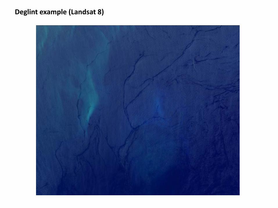
Deglint example (Landsat 8)

Deglint example (Landsat 8)

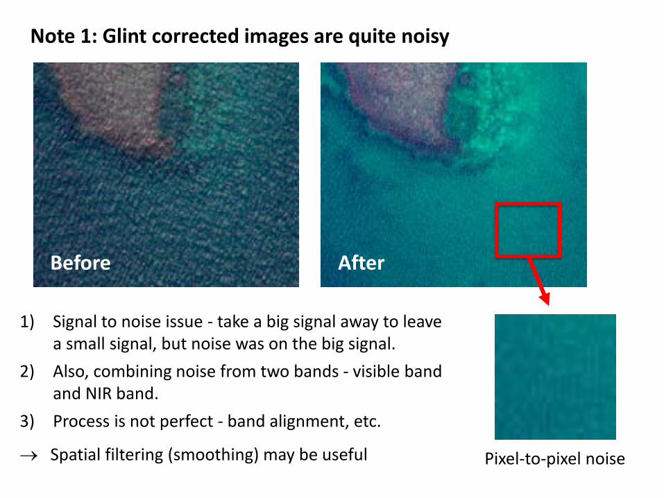
Note 1: Glint corrected images are quite noisy

1) Signal to noise issue - take a big signal away to leave a small signal, but noise was on the big signal.

2) Also, combining noise from two bands - visible band and NIR band.

3) Process is not perfect - band alignment, etc.

→ Spatial filtering (smoothing) may be useful

Before After

Pixel-to-pixel noise

Note 2: The need for precise band alignment • Image bands are not always perfectly spatially aligned • Causes serious problems for glint removal algorithm • WorldView-2 has various striping artefacts

• Sentinel-2 detector edges − similar problems

glint corrected band alignment on right side is bad

Note 3: Over-correction when NIR below surface is not zero • Assumption of zero NIR from below the water is not valid in shallow water • Result is “dark halo” effect around land features • Causes problems for subsequently applied algorithms

Before After

200 m × 200 m

3 m × 3 m

2 cm × 2 cm

1 km

High resolution sea surface model

Sea surface undulations occur at multiple scales • From 100’s metres to

millimetres • 10 m pixels may still contain

slopes contributing to the glint within them

Problem of sub-pixel glint (Sentinel-2)

Specific challenges with Sentinel-2 PIxel size means hard to get a “no glint” reference

The darkest pixels probably still contain some glint So glint correction is incomplete and there remains a glint contribution

Specific challenges with Sentinel-2 PIxel size means hard to get a “no glint” reference

Force correction to assume zero NIR reflectance rather than empirical minimum But that assumes NIR really should be zero - i.e. atmospheric correction has removed any aerosol contribution in the NIR - but atmospheric corrections often use NIR to estimate aerosol!

θs = 0 θv = 0

Atmospheric reflectance, Marine 99% RH aerosol model (libRadtran)

• In this plot sun and view are directly overhead (zenith and nadir) • Indirect surface reflectance but no direct glint included • Top two lines include aerosols, bottom line Rayleigh only

SWIR doesn’t help much - there still is an aerosol and glint contribution

Very difficult to disentangle glint from aerosol contribution in Sentinel-2 imagery - without additional information

aerosol contribution in NIR and SWIR

Harmel et al. 2018

• Glint correction for Sentinel-2 • Uses SWIR to characterise glint • Wavelength dependence based

on refractive index of water • But still relies on a-priori

separation of atmospheric reflectance from surface glint

Need this data for atmospheric correction, e.g. from AERONET station. Effectively this adds information to reduce uncertainty between aerosol and glint

Harmel T. et al. (2018) Remote Sensing of Environment, 204: 308-321 doi: 10.1016/j.rse.2017.10.022

Inversion methods for shallow water applications

Shallow water models for Rrs

1) HydroLight-EcoLight Build look-up tables for different depths, water column optical properties and bottom reflectances Mobley et al. (2005) Applied Optics 44, 3576-3592

2) Semi-analytical models Develop a simpler conceptual model and estimate coefficients or parameters from a physically exact model such as HydroLight Results in a forward model that is faster to compute Lee et al. (1998) Applied Optics 37, 6329-6338

Lee et al's semianalytical model for shallow water reflectance

H = depth in metres P = phytoplankton concentration (proxy) G = dissolved organic matter concentration (proxy) X = backscatter Y = (spectral slope of backscatter) is fixed at 1

remote sensing reflectance

bottom reflectance

Also incorporates sun and view zenith angles

Various factors derived from HydroLight

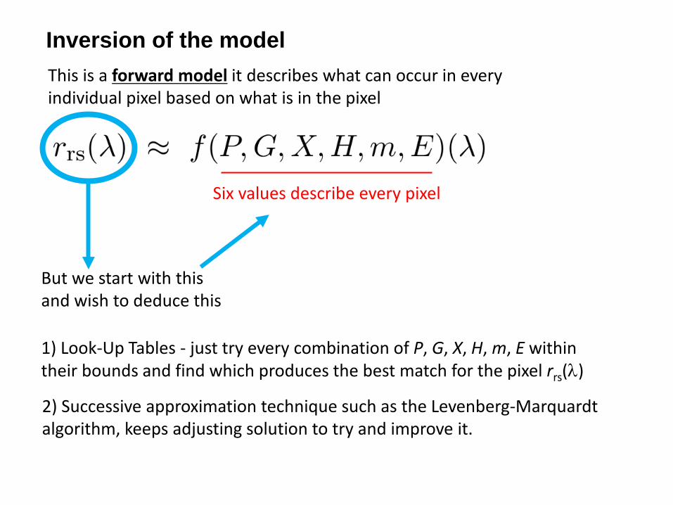
Inversion of the model This is a forward model it describes what can occur in every individual pixel based on what is in the pixel

Six values describe every pixel

But we start with this and wish to deduce this

1) Look-Up Tables - just try every combination of P, G, X, H, m, E within their bounds and find which produces the best match for the pixel rrs(λ)

2) Successive approximation technique such as the Levenberg-Marquardt algorithm, keeps adjusting solution to try and improve it.

LUT (look-up table)

Depth, Phytoplankton, CDOM, … etc 1 m 0.1 mg m-3

2 m 0.1 mg m-3

3 m 0.1 mg m-3

4 m 0.1 mg m-3

1 m 0.2 mg m-3

2 m 0.2 mg m-3

3 m 0.2 mg m-3

4 m 0.2 mg m-3

1 m 0.4 mg m-3

2 m 0.4 mg m-3

3 m 0.4 mg m-3

4 m 0.4 mg m-3

MODEL

Estimate: Depth = 2 m Phytopankton = 0.2 mg m-3

... etc

Image pixel

Adaptive LUT construction

Hedley et al. 2009, Remote Sens. Environ.

Example slice through ALUT structure

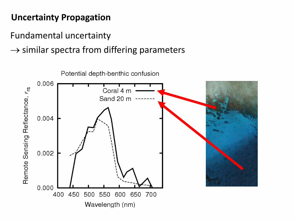
Fundamental uncertainty → similar spectra from differing parameters

Uncertainty Propagation

Sources of "noise" → uncertainty

model

"noise"

sensor

atmosphere

spectrally correlated

Hyperspectral deep water pixels

image noise

(multivariate normal)

subtract random noise term × 20 times

20 reflectance spectra

invert to retrieve parameter estimations

discard upper and lower tails to give

90% conf. intervals

Propagation through inversion Image pixel

use mean for actual result

• better than direct result • spatially smoother

Bathymetry estimation with uncertainty

CASI

Quickbird

= 90% confidence interval

0 m 300 m 100 m 200 m

Sentinel-2 bathymetry of Lizard Island (GBR) by model inversion

• Uses bands 1, 2, 3, 4 and 5 • ALUT inversion of Lee et al. equations • In-situ echo-sound data for comparison

Direct result (single inversion)

200 m

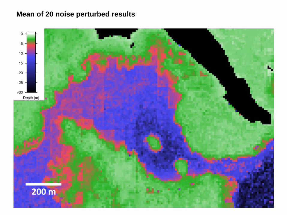
Mean of 20 noise perturbed results

200 m

Direct result (single inversion) Mean of 20 noise perturbed results

Single inversion vs. mean of noise perturbed inversions

• Marginally better statistics, r-squared, mean absolute residual, etc. • Cosmetically better (spatially smoother)

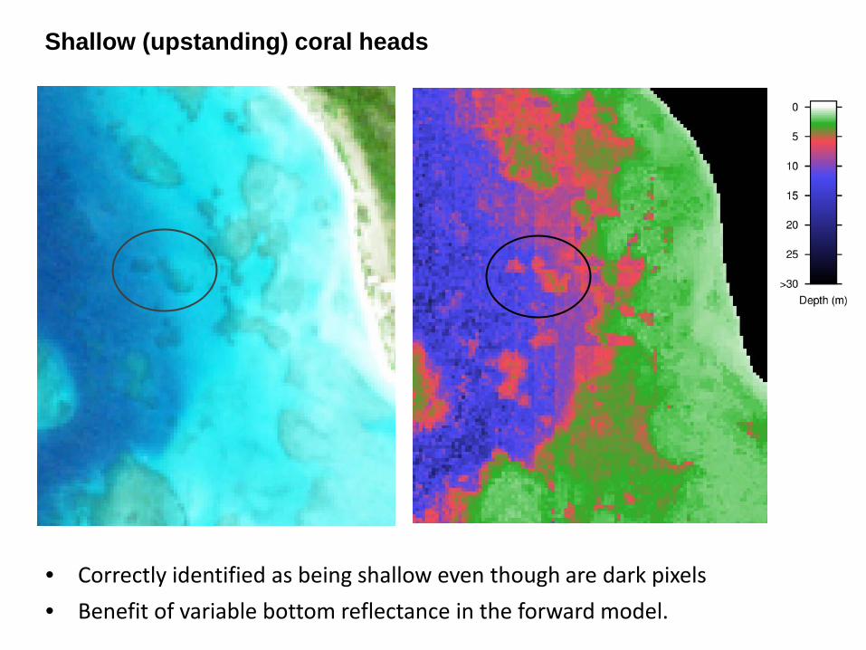
Shallow (upstanding) coral heads

• Correctly identified as being shallow even though are dark pixels • Benefit of variable bottom reflectance in the forward model.

Uncertainty (Quickbird image)

• Dark patches (coral heads) have relatively higher uncertainty in depth • Because there reflectance is similar to that of deeper pixels, within

the bounds defined by the noise model

Coral reef

Fish pens

Bolinao, Philippines (QuickBird image)

Light absorption due to CDOM Total absorption

Light absorption due to CDOM Total absorption

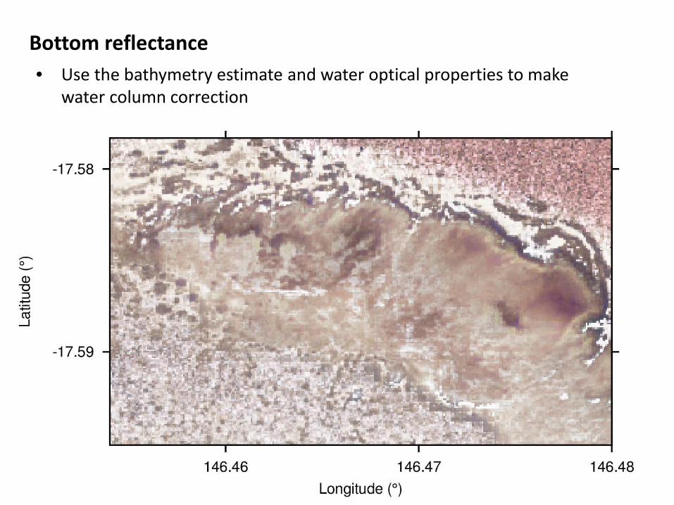
Bottom reflectance • Use the bathymetry estimate and water optical properties to make

water column correction

Bottom reflectance • Use the bathymetry estimate and water optical properties to make

water column correction

• Corals turn temporarily white when stressed by elevated temperature • Key indicator of climate change stresses on coral reefs

Coral Bleaching

(photo, P. Mumby)

Coral Bleaching Detection (Sentinel-2)

Coral Bleaching Detection (Sentinel-2)

Object-orientated / machine learning techniques

bottom reflectance

bathymetry

original image

environmental data (e.g. wave energy, wind)

habitat map

Sen2Coral Toolkit in SNAP

Sentinel Application Platform http://step.esa.int/main/toolboxes/snap/

Questions…