Shallow-water receptions from the transarctic acoustic propagation experiment

Shallow-water receptions from the transarctic acousticpropagation experiment

Richard Pawlowicz and David FarmerInstitute of Ocean Sciences, P.O. Box 6000, Sidney, British Columbia V8L 4B2, Canada

Barbara SotirinOcean and Atmospheric Sciences Division, NCCOSC-RDTE, San Diego, California 92152-6743

Siobhan OzardUniversity of Victoria, Victoria, British Columbia, Canada

~Received 10 October 1995; accepted for publication 27 February 1996!

In April 1994 a long-range, low-frequency acoustic propagation experiment took place in the Arcticto test the feasibility of using acoustic methods to observe large-scale thermal variability. Here thecharacteristics of the received signals at a vertical hydrophone array and a horizontal geophone arraylocated at the edge of the continental shelf in the Lincoln Sea, about 1 Mm from the source, arediscussed with respect to the ‘‘forward’’ problem of understanding and correctly modelingpropagation. Both cw~tonal! and tomographicM -sequence transmissions are analyzed. It is foundthat phase stability is very good, and that phase changes are almost entirely due to source/receivermotions. Travel times are not quite as stable, but are consistent with the phase observations,showing that phase can be used to measure travel time changes very accurately. Modaldecomposition ofM -sequence transmissions received by the vertical array shows an arrivalstructure in rough agreement with predictions from a coupled-mode calculation. Predictions usingan adiabatic approximation appear to work fairly well for modes 1 and 2, but not for higher-ordermodes which have significant bottom interaction, implying that accurate knowledge of thebathymetry is important in understanding and modeling the signals. Overall, it appears that theforward problem in the water column is known well enough to make an acoustic monitoringprogram feasible. The acoustic signals were also sensed by geophones placed on the surface of theice, but it appears that absolute phase and its spatial coherence across the geophone array~althoughnot time stability at any particular geophone! is greatly degraded by the large inhomogeneitiespresent in older ice. ©1996 Acoustical Society of America.

PACS numbers: 43.30.Qd, 43.30.Pc@JHM#

INTRODUCTION

The transarctic acoustic propagation~TAP! experimenttook place in April 1994.1 A high-power, low-frequencysource was located north of Svalbard at icecamp TURPAN,and made a number of hour-long cw~continuous wave ortonal! and tomographicM -sequence transmissions over a pe-riod of five days. These transmissions were heard at icecamps in both the Lincoln and Beaufort Seas. Here we ana-lyze transmissions received at icecamp NARWHAL whichwas situated at the edge of the continental shelf in the Lin-coln Sea~Fig. 1!, at a range of about 1 Mm from the source.

The purpose of this analysis is to provide some quanti-tative support for the idea that long-range acoustics can beusefully employed in the Arctic to observe changes in tem-perature structure. In pursuit of this aim, a number of tech-nical issues concerning the theory and practice of acousticpropagation will be addressed. An analysis of oceanographicquestions raised by this data will be treated in a subsequentpaper.

The analysis is divided into three parts. First, we de-scribe relevant details of the TAP experiment, beginningwith the acoustic environment. Second, we describe the char-acteristics of the received acoustic energy in the water col-umn. Particular attention will be paid to issues of robustness

with respect to various environmental parameters. Third, wedo the same for the more limited geophone data.

I. EXPERIMENT OVERVIEW

A. Acoustic environment

Although a detailed discussion of the oceanographicproperties of this region is beyond the scope of this paper, itis worthwhile to briefly describe the temperature field alongthis path, since sound-speed changes are most easily thoughtof as being related to temperature changes in the Arctic. Formore details, the reader is referred to other works.2,3 Thetemperature field is characterized by near-freezing waters inthe upper 100 m, overlying a warmer core of Atlantic water~AW! that cools and subducts in the Fram Strait. This tem-perature profile results in a shallow surface duct in thesound-speed field. Near the source location, the AW core hasa maximum temperature of almost 2 °C near 250 m. The AWcore then circles the Arctic, being modified by various ver-tical and horizontal mixing processes, finally reappearing atthe receiver location in the Lincoln Sea before continuingeastward toward Fram Strait and out of the Arctic. Thismodified core is colder~less than 0.5 °C!, less pronounced,and has a deeper temperature maximum~at about 500 m!

1482 1482J. Acoust. Soc. Am. 100 (3), September 1996 0001-4966/96/100(3)/1482/11/$10.00 © 1996 Acoustical Society of America

Downloaded 10 Sep 2013 to 128.197.27.9. Redistribution subject to ASA license or copyright; see http://asadl.org/terms

compared with the original core. The mid-point of the acous-tic path passes near the edge of Morris Jesup Plateau andskirts the edges of the Amundsen Basin. In this region, anAW core of intermediate warmth appears. Since tempera-tures decrease below the AW core, the possibility of a sound-speed minimum at a depth of'700 m exists. Such a channelappears near the source, but is far too weak to trap significantamounts of acoustic energy. Over most of the path soundspeeds increase monotonically with depth.

The source icecamp was located over the abyssal plainof the Nansen basin, in some 4000 m of water~Fig. 2!. Near

Morris Jessup Plateau the water depths decrease to about2500 m, remaining at around this value for another 400 kmor so. In the final 100 km of the path the seafloor shoalsrapidly, with slopes of up to 6° only 10 km away from thereceiver. The receiver ice camp was located near the 510 misobath at the edge of the continental shelf in the LincolnSea.

The entire path was bounded above by the Arctic icepack. Observed ice thicknesses near both the source and re-ceiver were about 4 m, although in general one expectssomewhat thicker ice north of Greenland than north of

FIG. 1. Location of the TAP path to the Lincoln Sea.

FIG. 2. Bathymetry and temperature along the TAP path~see text for details!. The dashed curve shows ETOPO5 bathymetry.

1483 1483J. Acoust. Soc. Am., Vol. 100, No. 3, September 1996 Pawlowicz et al.: Shallow-water receptions


Svalbard.4 Ice at the receiver was quite old, and in conse-quence the surface was very hummocky to the eye. The baseof the ice was also probably quite uneven, although this isuncertain since noin situ observations were made. Estimatesof ice parameters suitable for modeling purposes are listed inTable I. The values chosen are typical of those listed in pub-lished sources.4,5 Although not strictly necessary, we havefor simplicity assumed that these parameters are representa-tive of the entire path.

The temperature field used to generate sound speeds forpropagation modeling consists of a simple linear interpola-tion between measured profiles at the source and receiverlocations~Fig. 2!. Since measured profiles do not extend tomuch deeper than 500 m, at greater depths we take valuesfrom representative CTD stations occupied in 1991.6 Thesalinity field ~not shown! was similarly derived. These spa-tially smooth fields are somewhat similar to those obtainedfrom a coarse climatology,7 although they are different fromfields resulting from more recent ideas about the Arctic cir-culation which take into account the controlling effects ofbathymetry.3 However, they are sufficiently correct for theanalysis described here.

Accurate propagation modeling, especially at low fre-quencies in the shallow waters near the receiver, requires agood geoacoustic model of the seafloor. The bottom here istreated as a fluid, with sound speed and density parametersfor the upper 70 m taken fromin situobservations8,9 ~Fig. 3!.

A representative bottom attenuation of 0.003 dB m21 wastaken from the review by Hamilton.10

B. Ice camp TURPAN

The TAP source was located at ice camp TURPAN,which was in the vicinity of 83 °N latitude, 24 °E longitudeon 18 April 1994, and thereafter drifted roughly southwest-ward at a rate of about 10–15 km/day. Since this drift wasroughly perpendicular to the transmission path, the range de-crease due to source motion alone was only about 11 kmover the entire five-day period. Floe position was determinedusing a GPS receiver located 100 m from the source location.Unfortunately, no quantitative floe rotation observationswere made, although it is believed that the rotation was lessthan 30°, so that a small bias remains in source/receiverranges~this bias would be about 90610 m!. CTD profiles toa depth of about 600 m were taken every day.

Over the five days of the experiment, 43-h-long cw andtomographicM -sequence transmissions with a carrier fre-quency of 19.6 Hz were made using an experimental 195 dB~250 W! source suspended at a depth of 60 m. cw signalsconsist of a single sinusoid. TomographicM -sequences aresignals formed by modulating the phase of a carrier fre-quency in a pattern based on a pseudorandom number se-quence. Pulse compression at the receiver can be accom-plished by correlating the received signal with this samesequence. Using this technique, signal energy that is spreadout over a long period of time, and is below the ambientnoise level, can be mathematically converted into a shortpulse rising above the noise level.11

Transmissions were generally scheduled in a ‘‘1 houron, 1 ~or 2! hours off’’ scheme. The carrier phase was con-trolled by an atomic clock synchronized with GPS so thatdifferent transmissions can be coherently analyzed. How-ever, the modulation of phase used for tomographicM -sequence transmissions, although synchronized with thecarrier phase, was initiated manually~A. Gavrilov, personalcommunication 1995!, hence absolute travel times may be inerror by an integral number of carrier periods for a total errorof up to perhaps 1 s. With this design, theM -sequence phaseand its changes can be coherently compared with cw phaseand its changes, even though absolute travel times are notknown exactly.

During almost all of theM -sequence transmissions, theactual source signals were monitored.

In most cases it was found that the transmitted signalwas correct, but in some cases problems arose~probably dueto electrical interference in the source electronics! and digitswould be skipped at various points during the hour-longtransmissions. A summary of the transmissions discussedhere is given in Table II.

C. Ice camp NARWHAL

Ice camp NARWHAL was in the vicinity of 84 °N lati-tude, 63 °W longitude at the edge of the continental shelf inthe Lincoln Sea. The position of the ice camp was monitoredusing a GPS receiver. The camp was stationary until the 20thof April, after which it drifted northwestward at a speed of

TABLE I. Ice parameters used in propagation modeling.

Frequency 19.6 Hz

Compressional wave speedcp 3500 m s21

Compressional attenuationap 1.0 dB l21

Shear wave speedcs 1750 m s21

Shear attenuationas 1.0 dB l21

Ice thickness 4 mIce roughness 10 m2

Correlation length 22 m

FIG. 3. Geoacoustic model for the bottom in the Lincoln Sea.~a! Soundspeed and~b! density as a function of depth into the bottom.



1–2 km/day. Daily floe rotation observations showed that theorientation varied by only 1.5° over the course of the experi-ment. A CTD survey was carried out, so that sound-speedprofiles near the receiver are known. Instantaneous source/receiver separation distances on the WGS-84 spheroid werecalculated from the GPS positions. Horizontal refraction wasassumed to be unimportant.

Although both ice camps drifted quite far, their separa-tion decreased by only 9 km during the 5 days of the experi-ment ~a decrease of 11 km due to source drift alone waspartly compensated by a 2 kmincrease due to receiver drift!.Separation distances have an error of650 m due to noise inthe GPS-derived positions.

Two arrays were used to listen to the TAP transmis-sions. The most important was a vertical line array~VLA !suspended beneath the ice in 510 m of water. The VLA wasa light weight, low-power, analog-multiplexed system. Sen-sor outputs were digitized by an electro-optic node and trans-mitted via a fiber-optic link to a recording/control system.For the period discussed here, the useful portion of the arrayconsisted of 16 hydrophones spaced at 30.2-m intervals,spanning the entire water column and sampled at a nominalrate of 256 Hz. Time stamping was synchronized with GPStime.

The VLA was navigated during some periods with afour-beacon acoustic element localization~AEL! system,which provided estimates of horizontal displacements atthree points along the array every 5 min. VLA displacementsare dominated by tidally driven cycles, but the contributionsof other frequency components are not negligible.

A horizontal line array~HLA ! was also deployed. TheHLA consisted of nine geophones spaced 10 m apart, along aline which for the period discussed here was angled about 20deg from the expected direction of the source. Of the ninegeophones, seven were single vertical channel models. Twowere three-axis geophones, each consisting of three single-axis geophones mounted orthogonally in a frame. Perfor-mance of these three-axis phones, quantified by studying am-bient noise and the results of ‘‘light bulb drop’’ tests, wasnot entirely satisfactory; in particular the horizontal channelsof geophone one returned no useful information. The orien-tation of the horizontal channels was not recorded. Geophone

signals were sampled at a nominal 2010.816 Hz, althoughthe clock used for timing was of low quality, being neithersynchronized with the VLA clock nor particularly stable.Further timing problems arise because the time stamping ofdata files is accurate only to the nearest second, so that co-herent processing across files is not possible. This problem isintensified by some problems with the data acquisition sys-tem, which was often disrupted, apparently by electrical tran-sients produced by nearby equipment, so that there are fewlong uninterrupted segments of recorded data. This is a se-vere constraint when attempting to processM -sequencetransmissions.

Because of other experiments being conducted, onlyparts of the complete TAP transmission sequence were re-corded. Most of the recorded VLA receptions do not coin-cide with the periods for which the array was navigated.Although at first glance it appeared that the array displace-ment could be well modeled by a tidal cycle, further analysisindicated that abrupt motions of the ice camp and some com-plexities in the current field visible in ADCP records for theupper 100 m.~A. Plueddemann, WHOI, personal communi-cation, 1995! would make such extrapolations rather unreli-able. Finally, the HLA was not continuously monitored, sothat disruptions sometimes resulted in long gaps before thesystem was restarted. There is very little overlap between thevarious datasets, and our discussion will necessarily consistof ‘‘best examples’’ of various phenomena.

II. THE TAP TRANSMISSIONS: VERTICAL ARRAY

A. Data processing

The recorded data from each channel in the VLA wereprocessed independently. Gain corrections from predeploy-ment calibration curves were applied; this procedure appearsto be accurate within about 2 dB based on an analysis ofambient noise. Data were processed in 20-min blocks, withoverlapping segments added from previous and trailingblocks. Data blocks were first processed by filtering outspikes and then removing any mean offset. Spike removalwas sometimes necessary to remove contamination withhigh-frequency AEL transmissions, and consisted of a gatedrunning median filter. The data were then complex demodu-lated using the nominal carrier frequency~19.6 Hz! with noDoppler correction. Camp drift rates are sufficiently smallthat the signal degradation inM -sequence processing due toneglect of Doppler is negligible. Since source transmissionswere coherently timed using an atomic clock, the carrierphase is coherent between different transmissions. Demodu-lated data was low-pass filtered in both directions using aChebyshev filter with a cutoff at about 3 Hz. After filtering,the data were decimated by a factor of 10. No further pro-cessing was applied to cw transmissions.M -sequence trans-missions were further processed by correlation with the se-quence replica, after removal of a mean.

B. Arrival patterns: Observations

Figure 4~a! shows a coherent average over eight recep-tions from transmission T19 in the form of a time/depth plot.T19 is a useful transmission for our purposes since, although

TABLE II. TAP transmissions discussed in the text. Transmission types areeither cw for tonal, or MXXX/YY signifying anM -sequence transmissionwith sequence length XXX and YY cycles per digit. All transmissions havea carrier frequency of 19.6 Hz.

NameDate

~April 1994!Time

~GMT! Type Notes

T17 19 2200–2300 M255/12.5T19 20 0400–0500 M255/12.5 Phase jumps, missing digitsT29 21 0400–0500 cwT36 21 1900–2000 cwT37 21 2200–2300 cwT38 22 0100–0200 cw 20 min only, phase jump.T39 22 0400–0500 cwT40 22 0700–0800 cwT41 22 0900–1000 M127/12.5T42 22 1100–1200 cw



the source had some problems~see Table II!, array naviga-tion and geophone data were available. The arrival patternconsists of a large-amplitude pulse heard at all phones, fol-lowed some 6 s later by a smaller peak that appears mostly inthe upper half of the water column. Between the two peaks isa period of rather unorganized energy, definitely above am-bient noise levels but not showing any clearly identifiablepeaks. Figure 4~b! shows the magnitude of the received sig-nal at all 16 phones in the form of time series. The TAPsignal clearly appears at all hydrophones. Figure 4~c! showsa modal decomposition of this signal. The early peak con-sists primarily of mode 2, with other contributions mostlyfrom modes 3 and 4. The trailing peak consists only of mode1. The rather dispersed energy between these two peaks ap-parently consists mostly of mode 2.

C. Arrival patterns: Forward modeling

In order to better understand this structure, we attempt toduplicate it using a propagation model. Ray theory is notuseful here because we are dealing with a low-frequencysignal composed of only a few modes. Calculations based onray theory~not shown! do a very bad job in localizing thetrailing mode 1 peak and showing the structure of the leadingmultimode peak, although the results are consistent with ac-tual observations within the limitations of ray theory. In-stead, we must rely on a full-wave theory, and we choosehere to use the normal-mode method as implemented in thecomputer codeKRAKEN.12

The normal-mode approach to propagation modeling hastwo distinct subclasses.13 A rigorous general solution re-quires mode coupling effects to be included, which can bedone by approximating a fully range-dependent environment

with a grid of short range-independent segments.14 In manycases when range dependence is ‘‘not too strong,’’ an adia-batic approximation15 in which no energy is exchanged be-tween different modes is both reasonably accurate and com-putationally faster since it can be done with a coarser gridspacing. An adiabatic approximation also considerably sim-plifies the formal structure of a modal inverse, since the vari-ous modal travel times can be treated independently of oneanother. Both fully coupled and adiabatic solutions werecomputed. For the calculations shown here, the range wasdivided into 376 steps, with spacings of 330 m over the last120 km when depths were less than 2000 m and depthchanges rapid enough that significant bottom interactions oc-cur. Grid spacing is somewhat greater over eastern parts ofthe path nearer the source when bottom interactions are un-important. Since increasing the number of range steps to 600resulted in virtually no change for adiabatic calculations andonly small changes in the higher-order modes in coupledcalculations, the results were judged to be sufficiently accu-rate for our purposes. Gaussian pulse propagation was mod-eled using Fourier synthesis over 29 frequencies. AlthoughKRAKEN solves a flat-earth problem, correction for the sphe-ricity of the Earth was made by adjusting the sound-speedprofile. The travel-time decrease due to this correction isabout 0.1 s.

Using the linearly interpolated sound-speed profiles de-rived from the temperature field shown in Fig. 2 and the iceparameters in Table I, we first attempt to match the relativeamplitudes between various modes using the standard scat-tering mechanisms contained inKRAKEN. These include aKirchhoff scattering approximation, the Twersky soft-bosstheory, and an interfacial roughness matching condition. Inall cases, the amplitude of the trailing mode 1 peak was fartoo large relative to the initial peak. Best results were foundusing the elastic scattering theory of LePage and Schmidt,16

modified ~B. Tracey, MIT, personal communication, 1994!by the inclusion of attenuation within the ice. Since the lead-ing pulse is composed of a number of modes, its shape isvery sensitive to the phase of the received modes~i.e., onmodal interference!, and it is more useful to compare modaldecompositions rather than the raw pressure field.

Figure 5~a! shows the results of a coupled-mode calcu-lation, and Fig. 5~b! shows the results for an adiabatic calcu-lation, using range and bathymetry suitable for T19. Thisfigure should be compared directly with Fig. 4~c!.

Both calculations are broadly similar to the data, in thatthey each show a large initial peak composed of a number ofmodes, followed some 6 s later by a small mode 1 peak. Thelate arrival of mode 1 occurs because it is trapped in theshallow surface duct. The nearly simultaneous arrival ofmodes 2 and higher is a little unexpected, since in a canoni-cal Arctic profile where the sound speed increases withdepth, the higher-numbered modes propagate faster. How-ever, over this path bottom effects are important, and in shal-low water the lowest numbered modes are fastest. That is,the effects of shallow bottom interaction cancel the effects ofsound speed increases with depth for higher-order modesover this path.

The difference between the coupled and the adiabatic

FIG. 4. Sample arrival for T19. Eight sequences have been coherently av-eraged together in this figure.~a! Amplitude of received signal as a functionof depth and time. Ocean bottom is indicated by thick solid line, note thatthe acoustic energy penetrates into the bottom.~b! Time series of amplitudeat all phones.~c! Modal decomposition of the received signal~d! An esti-mate of an ‘‘ideal’’ geophone signal based on estimating the vertical deriva-tive using the uppermost hydrophones.



calculation is quite marked for modes 3 and higher, althoughan adiabatic approximation appears to work well for modes 1and 2 which do not interact strongly with the bottom. Highermodes which appear in the adiabatic calculation tend to van-ish in the coupled calculation, similar to the pattern seen inthe observations, because much of this energy actuallypropagates into the bottom and is lost. Modal peaks in thetwo calculations also differ in travel time, especially formodes numbered higher than 2.

D. Bathymetry

Since bottom interactions are so important in determin-ing the arrival pattern, it is necessary to include correctbathymetry into the forward model. It turns out that the con-venient ETOPO5 database is not accurate enough to cor-rectly model the slope features near the Lincoln Sea, prima-rily because it severely underestimates the slope of thecontinental shelf~Fig. 2!. This is especially critical here be-cause the acoustic path generally traverses the slope at a veryshallow angle. Instead, values from US Navy charts wereused. Figure 5~d! shows the results of a coupled mode cal-culation using the ETOPO5 bathymetry. Travel times andamplitudes for modes 2 and higher differ from those in Fig.5~a!. Unfortunately, this difference does not in itself validatethe use of the charted depths, it merely points out that accu-rate bathymetry is quite important.

E. Time stability of signal amplitude

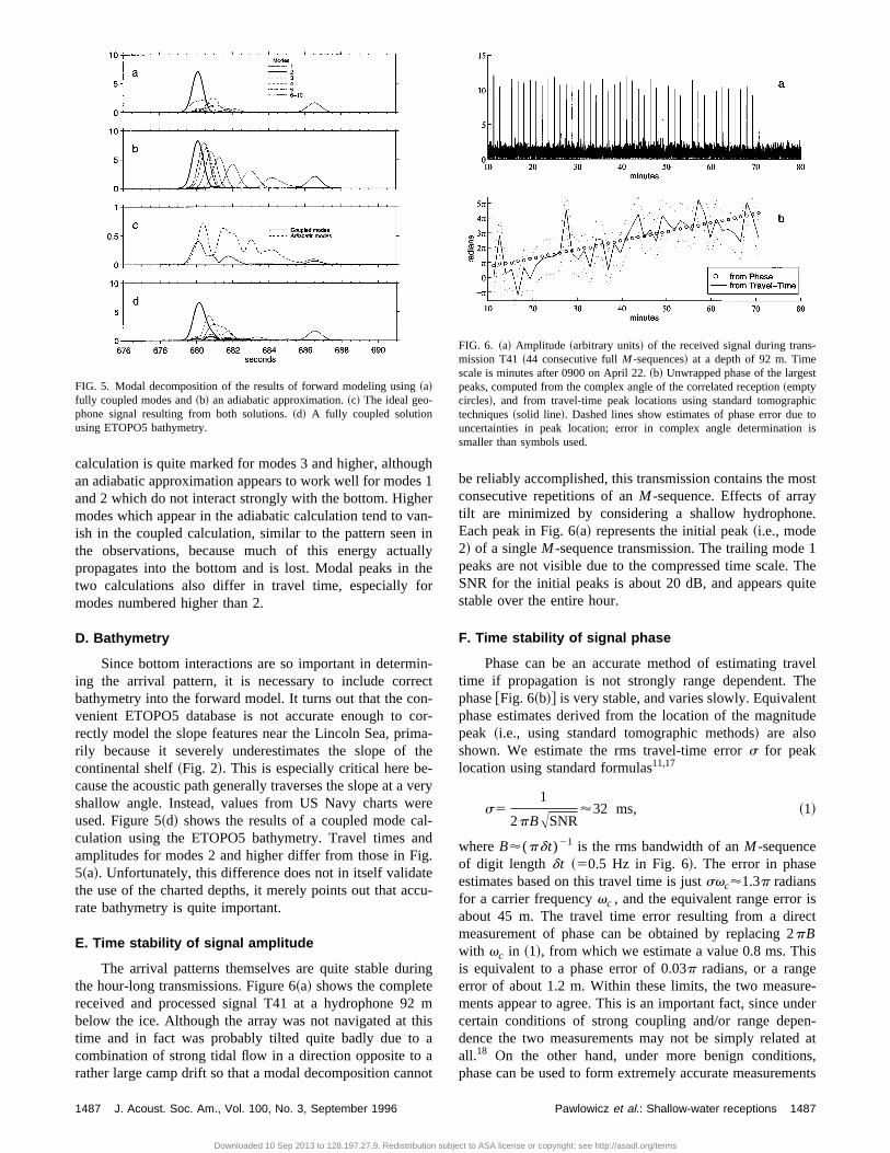
The arrival patterns themselves are quite stable duringthe hour-long transmissions. Figure 6~a! shows the completereceived and processed signal T41 at a hydrophone 92 mbelow the ice. Although the array was not navigated at thistime and in fact was probably tilted quite badly due to acombination of strong tidal flow in a direction opposite to arather large camp drift so that a modal decomposition cannot

be reliably accomplished, this transmission contains the mostconsecutive repetitions of anM -sequence. Effects of arraytilt are minimized by considering a shallow hydrophone.Each peak in Fig. 6~a! represents the initial peak~i.e., mode2! of a singleM -sequence transmission. The trailing mode 1peaks are not visible due to the compressed time scale. TheSNR for the initial peaks is about 20 dB, and appears quitestable over the entire hour.

F. Time stability of signal phase

Phase can be an accurate method of estimating traveltime if propagation is not strongly range dependent. Thephase@Fig. 6~b!# is very stable, and varies slowly. Equivalentphase estimates derived from the location of the magnitudepeak ~i.e., using standard tomographic methods! are alsoshown. We estimate the rms travel-time errors for peaklocation using standard formulas11,17

s51

2pBASNR'32 ms, ~1!

whereB'(pdt)21 is the rms bandwidth of anM -sequenceof digit length dt ~50.5 Hz in Fig. 6!. The error in phaseestimates based on this travel time is justsvc'1.3p radiansfor a carrier frequencyvc , and the equivalent range error isabout 45 m. The travel time error resulting from a directmeasurement of phase can be obtained by replacing 2pBwith vc in ~1!, from which we estimate a value 0.8 ms. Thisis equivalent to a phase error of 0.03p radians, or a rangeerror of about 1.2 m. Within these limits, the two measure-ments appear to agree. This is an important fact, since undercertain conditions of strong coupling and/or range depen-dence the two measurements may not be simply related atall.18 On the other hand, under more benign conditions,phase can be used to form extremely accurate measurements

FIG. 5. Modal decomposition of the results of forward modeling using~a!fully coupled modes and~b! an adiabatic approximation.~c! The ideal geo-phone signal resulting from both solutions.~d! A fully coupled solutionusing ETOPO5 bathymetry.

FIG. 6. ~a! Amplitude ~arbitrary units! of the received signal during trans-mission T41~44 consecutive fullM -sequences! at a depth of 92 m. Timescale is minutes after 0900 on April 22.~b! Unwrapped phase of the largestpeaks, computed from the complex angle of the correlated reception~emptycircles!, and from travel-time peak locations using standard tomographictechniques~solid line!. Dashed lines show estimates of phase error due touncertainties in peak location; error in complex angle determination issmaller than symbols used.



of travel-time changes. Here, the marginal consistency of thetwo measurements is probably an effect of the dominance ofthe adiabatic mode 2 arrival in the initial peak.

But just what is the phase telling us? Figure 7 shows acomparison between the phase of the TAP transmissionsT36–T42 over a 20-h period during April 21–22 with GPS-derived range changes. For demodulated cw transmissions,we have a relationship between slow phase changesDF andhorizontal range increasesDr of

2DF

2p•l5Dr , ~2!

wherel'76 m is the horizontal wavelength of the dominantlow-order modes. We use this relationship to compare phasechanges with range changes. There is a 2p ambiguity in thiscomparison which appears in the figure as striping.M -sequence phase is determined from the phase of the larg-est peak after sequence removal~as in Fig. 6! and has noambiguity. All transmissions in this figure are coherent, sothat the only free parameter is an arbitrary range offset. Theacoustic measurement of phase tracks the range changes al-most perfectly. In fact, it appears to do so more accuratelythan the raw GPS-derived ranges which have a650-m error.Range changes during this period are due to the drift of boththe source and receiver locations.

Note that the measured phase is a weighted sum of thephase of various modes. Although this sum is probablydominated by the contribution due to mode 2, the effects ofother modes are not necessarily negligible. These othermodes could have some effect on the absolute value of themeasured phase, but their effects on the changes of phase

with range would not become significant until the rangevariation approached intermodal interference distances, thatis, about 1 km or so.

A small travel-time/phase change due to the tides mightbe expected.19 An along-path tidal current of 1 cm/s wouldproduce a phase change of about 0.2p, equivalent to a rangechange of about 7 m. Although the accuracy of the positionestimates available for this experiment is unfortunately notenough to unambiguously determine the presence or absenceof such a signal, there is no technical reason preventing fu-ture experiments from doing so.

III. THE TAP TRANSMISSIONS: HORIZONTAL ARRAY

Since the true power of tomographic methods ariseswhen many acoustic paths are used, the possibility of obtain-ing useful measurements with a low-cost and relativelysimple receiving device is of great interest. Such a tool opensthe possibility of covering a substantial portion of the Arcticwith receivers. Geophones are certainly rather simple to de-ploy, and could easily be incorporated into expendable in-struments, telemetering their data via some satellite system.If horizontal angle-of-arrival information is desired, then ahorizontal array of geophones could be deployed much moreeasily than a horizontal hydrophone array. A horizontal geo-phone array was deployed for part of the TAP schedule, andwe shall now examine the measurements obtained from thisHLA.

A. Data processing

Data processing for the HLA proceeds in a similar fash-ion to that for the VLA. The signals are first low-pass filteredand subsampled by a factor 10 to make the amount of datamore manageable. For cw processing, the resulting signalsare complex demodulated and again low-pass filtered to re-move frequencies above 0.15 Hz. After this processing, thereremains a residual phase drift due to the unknown clock driftas well as source/receiver motions. This was modeled as aconstant and removed by fitting over all channels when nec-essary. InM -sequence processing, the complex demodulateswere correlated with the sequence replicas, low-pass filteredto a bandwidth of about 3 Hz, and then decimated again.

B. Comparison of geophone and hydrophone data

The geophones sense displacements in the ice at the fre-quencies being considered here, whereas hydrophones sensethe ambient pressure field. Predicting the geophone signaldue to a given acoustic source in the water column is ingeneral a complicated problem, requiring knowledge of thedynamics of an elastic medium~the ice! and its coupling tothe water column. However, we have a simpler problemhere: knowing what the observed~total! pressure field isclose to the base of the ice, we merely need to relate this tothe motions at the top of the ice.

First, using a narrow-band approximation and droppingthe exp$2ivct% dependence, vertical displacementsa(t) inthe water column are related to the vertical gradients in theobserved pressure fieldp(t) through mass conservation~i.e.,first principles! in the following way:

FIG. 7. Phase for transmissions T36–T42 during 21–22 April, comparedwith instantaneous range, after subtraction of'1 Mm. Phase estimates areindicated by dots which form coherent bands when the TAP signal is beingreceived. During periods when no TAP signal is received the phase is ran-dom, creating vertical bars on either side of the coherent bands. The 2pambiguity of cw phase is indicated by the horizontal striping. There is nostriping for the phase derived fromM -sequence transmission T41 at 0900.Phase for the partial reception T38 at 0200 is not coherent with the otherreceptions due to as-yet unresolved source problems sometime after 0100,however, its trend is meaningful.



a~ t !'1

rvc2

]p~ t !

]z. ~3!

We estimate this displacement by taking the difference be-tween the received signals at the upper two hydrophones.Assuming the validity of such a finite difference approxima-tion implicitly relies on the belief that the ice sheet is smoothon scales of the hydrophone spacing and smaller. Verticaldisplacements at the base of the ice sheet should exactlymatch the vertical water column displacements at the surface~the kinematic boundary condition!. Finally, at low frequen-cies the ice response is primarily in the antisymmetric mode~i.e., flexural waves! so that vertical displacements at the topof the ice are similar to those at the base. Analysis using atheory of transmission coefficients in a thin plate20 confirmsthat the TAP transmission frequency of 19.6 Hz is lowenough for this to be true. Note that since higher-ordermodes in general have larger derivatives near the surface,~3!implies that they will appear larger in geophone data than inhydrophone data. This ‘‘ideal’’ geophone signal is shown inFig. 4~d! for T19, and in Fig. 5~c! for the results of theforward model. The effects of nonadiabatic propagation~which are more important for the higher-order modes! areeven more marked in geophone data than in the hydrophonedata.

Assuming the ice is smooth, there should be no couplinginto horizontally polarized shear (SH) waves. Also, the low-order modes have propagation angles that are much shal-lower than the critical angle for generating longitudinal (P)waves. Thus we expect to hear TAP signals on the verticalchannels of the geophone array, but not on the horizontalchannels.

Figure 8 shows a comparison of geophone and hydro-phone data for T19. Hydrophone and geophone records werealigned by eye. Figure 8~a! shows a coherent average of nineM -sequences~after removing motion and clock drift effects!,and Fig. 8~b! shows traces of the phase information for allsequences used in the coherent average. The peaks in themagnitude plot coincide with periods of coherent phase andvice versa. It is interesting that although the arrival patternsare quite stable at any particular geophone, they vary quitesignificantly between the various channels. Channel 1 ap-pears to be most similar to the results predicted from thehydrophone data, but almost no sign of a signal can be seenin Fig. 8~a! for channel 5~the coherent phase for that channelshown in Fig. 8~b! indicates that there is in fact a signalthere!. Note also that the horizontal channels 8X and 8Yshow peaks that slightly trail the main peaks in the verticalchannels, indicating the presence of eitherP or SH waves,propagating either out-of-plane or at a different speed thanthe water-borne signal. Coupling of water-borne acoustic en-ergy through an apparently smooth ice surface intoSHwaves has been observed before.21

Mode 1 is too weak to be identified in almost all cases.The variability among geophones is in fact greater than thatshown, since the plotted curves have been normalized byambient noise levels which vary by up to a factor of 20among the various phones, being lowest for channels 3 and 9and highest for 5 and 6. In general, the SNR is slightly lower

for the geophone data than for the hydrophone data. It is notclear how general this feature is, since the geophone signalwas dominated by a broad spectral peak in the range 2–5 Hz.The origin of this peak is uncertain.

C. Stability of geophone signals

The dramatic differences between the various geophonechannels are puzzling. Forward modeling indicates thatchanges in the structure of the acoustic signal in the watercolumn over the distance spanned by the array are very small~this should be expected because the aperture of the HLA isfar smaller than the intermodal interference distance!. Figure9 shows results from T17 only 6 h previously in the sameformat as in Fig. 8~although no comparison with VLA datais possible here!. The path range was some 700 m less at thispoint than it was for T19. Again, we see quite stable arrivalpatterns within the various channels, and quite different pat-

FIG. 8. Geophone signals across the HLA during T19.~a! Amplitude infor-mation from all channels, as well as an ‘‘ideal’’ signal derived from thehydrophone data. EightM -sequences are coherently averaged, but all indi-vidual sequences fall within the shaded region.~b! Phase information fromall channels. Phase from each sequence is plotted separately, so that regionswhere a coherent signal is received are marked by overplotting, whereasphase is uniformly distributed over all angles during periods of ambientnoise.



terns between channels. However, a comparison with Fig. 8shows that the patterns at particular phones have changedquite a bit over 6 h, that is, there is a slow secular change inthe arrival pattern~in particular, note that there is a recog-nizable signal in channel 5!. These changes are similar inquality and size to those expected in the water column fromrange changes alone~not shown!.

One explanation for the differences between channels isthat the coupling of energy into the ice varies greatly overquite small scales, so that the assumption of horizontal uni-formity implied by the ‘‘ideal geophone’’ makes it a ratherbad model for the observed signal. Unfortunately we do notknow what the variability in ice thickness and acoustic char-acteristics was, but given the rough nature of the visible sur-face it is likely that the internal properties were also quitevariable spatially, and that the underside was also quiterough. Thus the acoustic field in the water column couldcouple not only into vertical motions using~3!, but also intohorizontal motions, possibly because of variations in icethickness~i.e., bending and twisting the ice sheet as well asjust lifting it!. Although these horizontal motions do not nec-essarily propagate as free waves, the effects of this couplingcan certainly affect the phase and amplitude of nearby verti-cal displacements. Horizontal displacements are observed inchannels 8X and 8Y, lending credence to this theory. Inter-ference patterns formed by these interactions would thenvary on the time scales of ice drift, which are primarily tidaland longer. This would explain the very stable arrival pat-terns which vary secularly over 6 h.

For completeness, we compare two different phase esti-mates for the peaks in the geophone data for T17~Fig. 10!.This figure should be compared directly with Fig. 6. In com-paring SNR, it should be noted that the signal processed inFig. 10 is a 255-digitM -sequence, whereas Fig. 6 shows theresults for a 127-digitM -sequence. Thus the comparableSNR for the geophone observations is about one half that ofthe hydrophone signals shown previously, although thisvalue is suspect due to temporal changes in ambient noiselevels. The peak amplitude appears to be less stable in thegeophone data than for the hydrophone data, although thephase estimates are of comparable quality.

The drastic loss of phase coherence across the array andthe unique character of each geophone’s signal appear toimply that any kind of coherent array processing is likely tobe of only marginal utility when geophones are deployedover rough ice. Figure 11 shows phase estimates across thearray for two cw transmissions. The expected phase variationdue to source/receiver geometry is indicated by a dotted line.The measured phases are quite different, varying by morethan 100° from expected values, and there are significantchanges in the pattern over time. Although the individualphase estimates are quite scattered, there appears to be atrend in phase across the array. If this were in fact a real

FIG. 9. Amplitude information for all geophone channels during T17, as inFig. 8 ~no comparison with VLA data is possible here!. See text for details. FIG. 10. ~a! Amplitude ~arbitrary units! of the received signal during

M -sequence transmission T17 at a geophone channel 4. Time scale is min-utes after 2200 on April 19.~b! Unwrapped phase of the largest peaks,computed from the complex angle of the correlated reception~emptycircles!, and from travel-time peak locations~solid line!. Dashed lines showestimates of phase error due to uncertainties in peak location. This figure canbe compared directly with Fig. 6. Although the SNR look similar in bothfigures, theM -sequence length here is 255 digits, twice the length of thatshown in the earlier figure. There is no data recorded before the 20-minmark, and a gap in the recorded data at 33 min.

FIG. 11. Phase estimates across the array during cw transmissions~a! T29and~b! T37. Dotted line represents expected phase variation. The measuredphases are inconsistent with these estimates, showing that coherent process-ing using the entire array is not possible.



trend, rather than an artifact of the physical processes caus-ing the phase ‘‘noise,’’ it would imply that the signal wasbeing received at an angle of about 20° to the north of theexpected angle. This value is far greater than the possiblegeometrical orientation error, and is opposite in direction topossible directional changes induced by sloping bathymetry.

It should noted that although useful coherent processingusing the array deployed here proved impossible, geophonearrays have been used successfully in other applications inorder to localize nearby sources and understand icewaves.5,21,22

IV. CONCLUSIONS

We have presented here some observations from thetransarctic acoustic propagation experiment. As has beenseen in previous experiments,23 phase is very stable in theArctic, and appears to change in time mainly as a function ofrange changes. In fact, phase changes are apparently a moreaccurate indicator of range changes than ranges derived fromraw GPS, although it is not clear how well this conclusionwould hold with GPS data post-processed to an accuracy of610 m or better. Indeed, one expects that tidal currents alonemight cause some travel time~hence phase! variability, asseen in long-range tomographic transmissions elsewhere.19

Travel times forM -sequence transmissions appear to be lessstable, although they are marginally consistent with phaseinformation. Thus the possibility of using phase informationin a tomographic scheme is worth considering.

It appears that the lower modes are perfectly capable ofpropagating up onto the shelf, and that reasonable signal-to-noise ratios can be achieved with existing technology. How-ever, bottom effects apparently result in the disappearance ofmodes numbered higher than 6, and severely affect the struc-ture of modes 3–6. Modes 1 and 2 appear to propagate al-most adiabatically. Accurate bathymetry is essential forproper modeling of the propagation of higher modes. Notconsidered here are the effects of bottom slope perpendicularto the acoustic path~Ref. 11, p. 168!. Since these effects aregreatest for the higher-numbered modes which are also thosemost attenuated by bottom interactions it is likely that theoverall effect is small, but further investigation is required.

Although only hydrophone arrays are generally consid-ered as components of tomographic systems, it appears thatgeophones might also be useful, since they appear to be ca-pable of sensing low-frequency signals in the water columnquite easily. Deployment of geophones, especially in hori-zontal arrays, could therefore be considered as a low-costmethod of providing receivers throughout the Arctic. How-ever, there are a number of drawbacks to the geophone datadiscussed here, and a number of practical issues that requirefurther investigation. It appears that phase and amplitude in-formation is badly affected by the inhomogeneities in oldand probably quite rough ice. This may not necessarily be aproblem for geophones deployed over smooth regions~refro-zen leads etc.!, although determining the exact specificationsthat such a smooth patch would have to meet requires furtherinvestigation. Even if absolute phase is adversely affected,phase changes may still be usable for tomographic purposes.

In general, signal-to-noise levels were more than ad-equate, implying that some relaxation of frequency/powerconstraints is possible in future experiments of this type.

ACKNOWLEDGMENTS

Our thanks to S. Dosso and J. Perkins~DREP! for pro-viding the geophone data, as well as Y. Xie~IOS! for dis-cussions about the acoustic nature of sea ice, B. Tracey~MIT ! for helping with the code for the elastic scatteringtheory, A. Mehrabian~SAIC! for answering questions aboutice camp TURPAN, A. Gavrilov~AcoustInform! for explain-ing the workings of the source electronics, J. Newton~PolarAssociates! for details of ice camp NARWHAL and the localbathymetry and B. Dushaw~APL/UW! for his questionabout tidally induced phase variability. This work is part of acollaborative study with P. Mikhalevsky~SAIC!, A. Bagge-roer, H. Schmidt~both MIT!, and M. Slavinsky, and wasmade possible by funding from Dr. T. Curtin at the Office ofNaval Research in the United States under Contract No.N-00014-95-1-0655.

1P. N. Mikhalevsky, A. B. Baggeroer, A. Gavrilov, and M. Slavinsky,‘‘Experiment tests use of acoustics to monitor temperature and ice inarctic ocean,’’ EOS, Trans. Am. Geophys. Union76~27!, 265, 268–269~1995!.

2E. C. Carmack, ‘‘Large-Scale Physical Oceanography of Polar Oceans,’’in Polar Oceanography Part A: Physical Science, edited by W. O. Smith~Academic, San Diego, California, 1990!, Chap. 4, pp. 171–222.

3R. Pawlowicz, ‘‘On historical temperatures north of Greenland,’’ DeepSea Res. Part A~in review! ~1996!.

4R. H. Bourke and A. S. McLaren, ‘‘Contour Mapping of Arctic Basin IceDraft and Roughness Parameters,’’ J. Geophys. Res.97~C11!, 17715–17728~1992!.

5T. C. Yang and G. R. Giellis, ‘‘Experimental characterization of elasticwaves in a floating ice sheet,’’ J. Acoust. Soc. Am.96, 2993–3009~1994!.

6L. G. Anderson, G. Bjo¨rk, O. Holby, E. P. Jones, G. Kattner, K. P. Kol-termann, B. Liljeblad, R. Lindgren, B. Rudels, and J. Swift, ‘‘Watermasses and circulation in the Eurasian Basin: Results from the Oden 91expedition,’’ J. Geophys. Res.99~C2!, 3273–3283~1994!.

7S. G. Gorshkov, ed.,Arctic Ocean, volume 3 ofWorld Ocean Atlas~Per-gamon, New York, 1983!.

8J. A. Hunter, J. M. Carson, R. A. Burns, and T. L. Good, ‘‘Compressionalwave velocity structure of the sub-bottom in the Lincoln Sea from verticalhydrophone array measurements,’’ Tech. Rep. Defense Research Estab-lishment Pacific, Victoria, B. C. Canada, April 1990.

9W. H. Geddes, ‘‘Geoacoustic model of the lincoln sea,’’ Tech. Rep.NOARL, March 1990.

10E. L. Hamilton, ‘‘Geoacoustic modeling of the sea floor,’’ J. Acoust. Soc.Am. 68, 1313–1340~1980!.

11W. Munk, P. Worcester, and C. Wunsch,Ocean Acoustic Tomography~Cambridge U. P., New York, 1995!.

12M. B. Porter, ‘‘The KRAKEN normal mode program,’’ Tech. Rep.,SACLANT Undersea Research Centre Memorandum~SM-245!/Naval Re-search Laboratory Mem. Rep. 6920, 1991.

13F. B. Jensen, W. A. Kuperman, M. B. Porter, and H. Schmidt,Computa-tional Ocean Acoustics~American Institute of Physics, Woodbury, NY,1994!.

14R. B. Evans, ‘‘A coupled mode solution for acoustic penetration in awaveguide with stepwise depth variations of a penetrable bottom,’’ J.Acoust. Soc. Am.74, 188–195~1983!.

15L. M. Brekhovskikh and Yu. P. Lysanov,Fundamentals of Ocean Acous-tics, volume 8 ofSpringer Series on Wave Phenomena~Springer-Verlag,Berlin, 1991!, Chap. 7, pp. 146–165, 2nd ed.

16K. LePage and H. Schmidt, ‘‘Modeling of low-frequency transmissionloss in the central arctic,’’ J. Acoust. Soc. Am.96, 1783–1795~1994!.

17P. F. Worcester, R. C. Spindel, and B. M. Howe, ‘‘Reciprocal acoustictransmissions: instrumentation for mesoscale monitoring of ocean cur-rents,’’ IEEE J. Ocean. Eng.OE-10~2!, 123–137~1985!.



18M. Dzieciuch and W. Munk, ‘‘Differential Doppler as a diagnostic,’’ J.Acoust. Soc. Am.96, 2414–2427~1994!.

19B. D. Dushaw, B. D. Cornuelle, P. F. Worcester, B. M. Howe, and D. S.Luther, ‘‘Barotropic and Baroclinic Tides in the Central North PacificOcean Determined from Long-Range Reciprocal Acoustic Transmis-sions,’’ J. Phys. Oceanogr. 631–647~1995!.

20Y. Xie and D. M. Farmer, ‘‘Acoustical radiation from thermally stressedsea ice,’’ J. Acoust. Soc. Am.89, 2215–2231~1991!.

21B. E. Miller and H. Schmidt, ‘‘Observation and inversion of seismo-acoustic waves in a complex arctic ice environment,’’ J. Acoust. Soc. Am.89, 1668–1685~1991!.

22Y. Xie and D. M. Farmer, ‘‘Seismic-acoustic sensing of sea ice wavemechanical properties,’’ J. Geophys. Res.99~C4!, 7771–7786~1994!.

23P. N. Mikhalevsky, ‘‘Characteristics of cw signals propagated under theice in the arctic,’’ J. Acoust. Soc. Am.70, 1717–1722~1981!.



Documents

Shallow-water receptions from the transarctic acoustic propagation experiment