Embed Size (px)
Citation preview
Shake Table ControlFidelity in Signal ReproductionFidelity in Signal Reproduction & Sources of Signal Distortion
Joel P. Conte, Professor, UCSDJ. Enrique Luco, Professor, UCSD
O O lik A i t t P f D k E l l U i T kOzgur Ozcelik, Assistant Professor, Dokuz Eylul Univ., Turkey
NEES@UNevada‐RenoNEES@UBuffaloNEES@UC San Diego
Shake Table Training Workshop 2010 – San Diego, CA
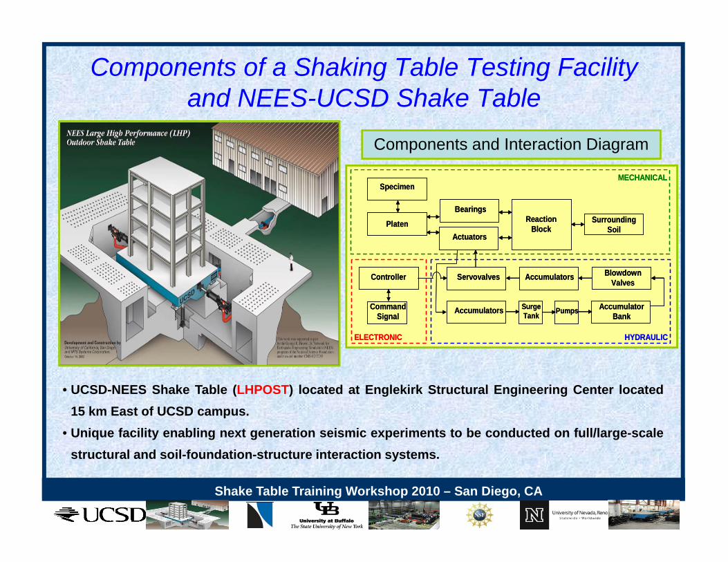
Components of a Shaking Table Testing Facilityand NEES-UCSD Shake Tableand NEES UCSD Shake Table
MECHANICALMECHANICAL
Components and Interaction Diagram
Specimen
PlatenActuators
BearingsSurrounding
SoilReaction
Block
MECHANICALSpecimen
PlatenActuators
BearingsSurrounding
SoilReaction
Block
MECHANICAL
Servovalves Accumulators BlowdownValves
Accumulators SurgeTank Pumps Accumulator
BankCommand
Signal
Controller Servovalves Accumulators BlowdownValves
Accumulators SurgeTank Pumps Accumulator
BankCommand
Signal
Controller
Tank BankSignal
ELECTRONIC HYDRAULIC
Tank BankSignal
ELECTRONIC HYDRAULIC
UCSD NEES Shake Table (LHPOST) located at Englekirk Structural Engineering Center located• UCSD-NEES Shake Table (LHPOST) located at Englekirk Structural Engineering Center located15 km East of UCSD campus.
• Unique facility enabling next generation seismic experiments to be conducted on full/large-scalestructural and soil-foundation-structure interaction systems.
Shake Table Training Workshop 2010 – San Diego, CA
structural and soil foundation structure interaction systems.
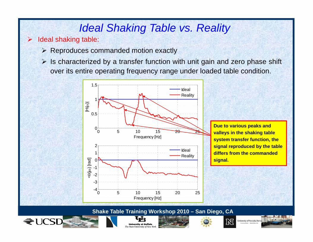
Ideal Shaking Table vs. Reality Ideal shaking table:
Reproduces commanded motion exactly Is characterized by a transfer function with unit gain and zero phase shift
over its entire operating frequency range under loaded table condition.
1
1.5
)|IdealReality
0 5 10 15 20 250
0.5
Frequency [Hz]
|H(
Due to various peaks and valleys in the shaking table
Frequency [Hz]
1
0
1
2
[rad]
IdealReality
system transfer function, the signal reproduced by the table differs from the commanded signal.
0 5 10 15 20 25-4
-3
-2
-1
Frequency [Hz]
< (j
)
Shake Table Training Workshop 2010 – San Diego, CA
Frequency [Hz]
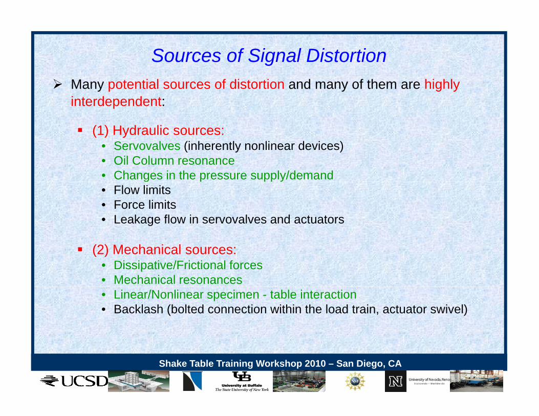
Sources of Signal Distortion Many potential sources of distortion and many of them are highly
interdependent:
(1) Hydraulic sources: (1) Hydraulic sources:• Servovalves (inherently nonlinear devices)• Oil Column resonance• Changes in the pressure supply/demandg y• Flow limits• Force limits• Leakage flow in servovalves and actuators
(2) Mechanical sources:• Dissipative/Frictional forces• Mechanical resonances• Linear/Nonlinear specimen - table interaction• Backlash (bolted connection within the load train, actuator swivel)
Shake Table Training Workshop 2010 – San Diego, CA

High-flow High-performanceServovalves
Pilot Stage3 t
3rd Stage
4 t
3-stage Servovalve
th
4-stage Servovalve
4th Stage
Load flow ports(port windows)
Main pressureentrance
Courtesy of MTSSystems Inc
Shake Table Training Workshop 2010 – San Diego, CA
Systems Inc.

Hydraulic - ServovalvesActuator Extent DirectionActuator Extent Direction Actuator Retract DirectionActuator Retract Direction
SP
P
vxActuator Extent Direction
SP
P
vxActuator Extent Direction
SP
P
vx
Actuator Retract Direction
SP
P
vx
Actuator Retract Direction
K Fl i (li i d fl ffi i t)
2P
V
1A2A
RP1 2
1P2P
V
1A2A
RP1 2
1P 1A2A
RP 3 4
1P2P
V
1A2A
RP 3 4
1P2P
V
1 1 1 1v v Sq A V K w x P P
2 2 2 2v v Rq A V K w x P P xv : 4th stage valve spool displacement.
Kv : Flow gain (linearized flow coefficient)wi : Valve port window widthsA1, A2 : The tension and compression areas
3 1 3 1v v Rq A V K w x P P
4 2 4 2v v Sq A V K w x P P v
1 2and P P
1 2and P P
Ps , PR : Supply and return system pressures.
: Actuator chamber pressures during extent direction.
: Actuator chamber pressures during retract direction.
Servo-valve flows present two independent sources of nonlinearity:• Load pressure nonlinearity or pressure drop - flow nonlinearity (explicitly represented by the square root term),
• Flow gain nonlinearity (Kv changes due to variable size orifice)
Shake Table Training Workshop 2010 – San Diego, CA
g y ( v g )
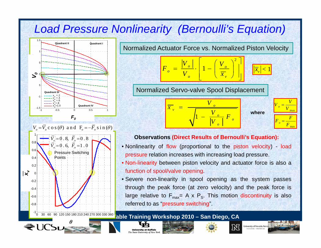
Load Pressure Nonlinearity (Bernoulli’s Equation)N li d A t t F N li d Pi t V l it
1.5y y y
Quadrant IQuadrant II
Normalized Actuator Force vs. Normalized Piston Velocity2
1o oo
o v
V VFV x
1vx <0
0.5
1
uato
r Pis
ton
Vel
ocity
V 0 o v
Normalized Servo-valve Spool Displacement
oVx oVV
V
-1 5
-1
-0.5
Nor
mal
ized
Act
u
xv =.2xv =.4xv =.6xv=.8xv=1.0
Quadrant III
Quadrant IV
V
Observations (Direct Results of Bernoulli’s Equation):
1v
oo
o
xV FV
where maxV
maxo
FFF
-1 -0.5 0 0.5 11.5
Normalized Actuator Force
F0
1
c o s ( ) a n d F s i n ( )o o o oV V F
0 . 8, 0 . 8V F ( q )• Nonlinearity of flow (proportional to the piston velocity) - load
pressure relation increases with increasing load pressure.• Non-linearity between piston velocity and actuator force is also a
function of spool/valve opening0.2
0.4
0.6
0.80 . 8, 0 . 8o oV F0 . 6, 1 . 0o oV F
Pressure Switching Points
v function of spool/valve opening.• Severe non-linearity in spool opening as the system passes
through the peak force (at zero velocity) and the peak force islarge relative to Fmax= A x PS. This motion discontinuity is also
f d t “ it hi ”-0.6
-0.4
-0.2
0x v
Shake Table Training Workshop 2010 – San Diego, CA
referred to as “pressure switching”.
0 30 60 90 120 150 180 210 240 270 300 330 360-1
-0.8
θ
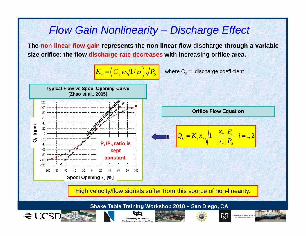
Th li fl i t th li fl di h th h i bl
Flow Gain Nonlinearity – Discharge Effect
1/ SdK wC P
The non-linear flow gain represents the non-linear flow discharge through a variablesize orifice: the flow discharge rate decreases with increasing orifice area.
where Cd = discharge coefficient 1/v SdK wC P d g
Typical Flow vs Spool Opening Curve (Zhao et al., 2005)
Lx P
Orifice Flow Equation
gpm
]
1 1,2v LL v v
v S
x PQ K x ix P
QL
[g
PL/PS ratio is kept
constant.
High velocity/flow signals suffer from this source of non-linearity.
Spool Opening xv [%]
Shake Table Training Workshop 2010 – San Diego, CA
High velocity/flow signals suffer from this source of non linearity.
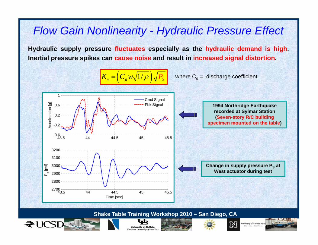
Flow Gain Nonlinearity - Hydraulic Pressure Effect
1/K C w P
Hydraulic supply pressure fluctuates especially as the hydraulic demand is high.Inertial pressure spikes can cause noise and result in increased signal distortion.
where C = discharge coefficient 1/v SdK C w P
1994 Northridge Earthquake0.6
1
[g] Cmd Signal
Fbk Signal
where Cd = discharge coefficient
1994 Northridge Earthquake recorded at Sylmar Station (Seven-story R/C building
specimen mounted on the table)
43 5 44 44 5 45 45 5-0.6
-0.2
0.2
Acc
eler
atio
n
43.5 44 44.5 45 45.5
3000
3100
3200
psi] Change in supply pressure PS at
43.5 44 44.5 45 45.52700
2800
2900
Time [sec]
Ps [p West actuator during test
Shake Table Training Workshop 2010 – San Diego, CA
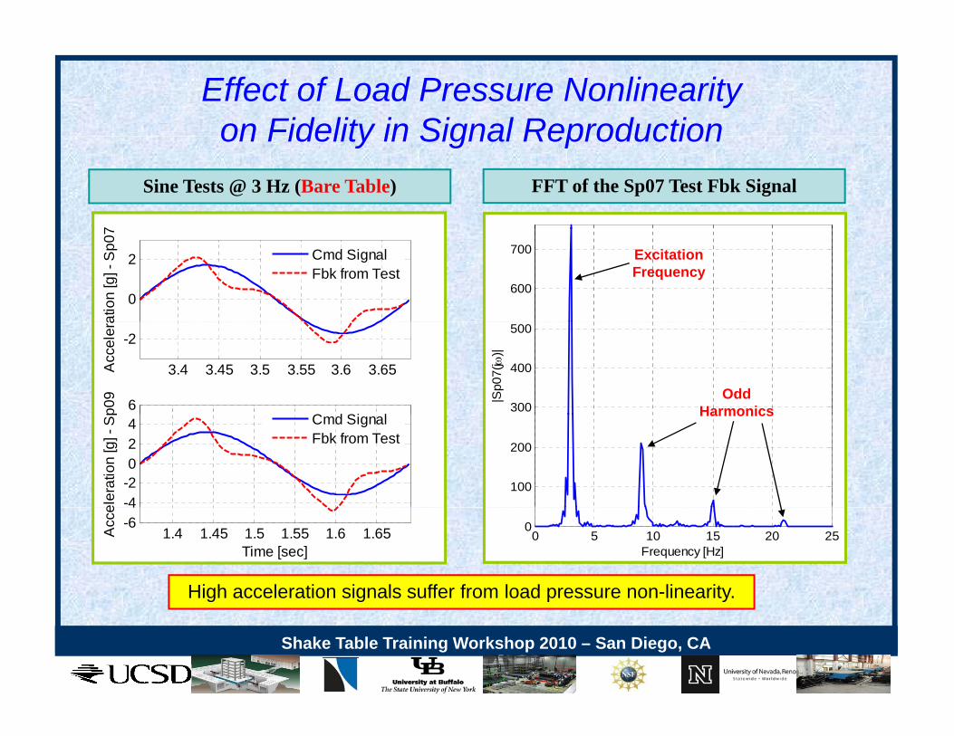
Effect of Load Pressure Nonlinearityon Fidelity in Signal Reproduction
Sine Tests @ 3 Hz (Bare Table)
7
FFT of the Sp07 Test Fbk Signal
on Fidelity in Signal Reproduction
0
2
atio
n [g
] - S
p07
Cmd SignalFbk from Test
600
700 ExcitationFrequency
3.4 3.45 3.5 3.55 3.6 3.65
-2
Acc
eler
a
6p09
C d Si l300
400
500
|Sp0
7(j
)|
OddHarmonics
-4-2024
eler
atio
n [g
] - S
p Cmd SignalFbk from Test
100
200
Harmonics
1.4 1.45 1.5 1.55 1.6 1.65-64
Time [sec]
Acc
e
0 5 10 15 20 250
Frequency [Hz]
High acceleration signals suffer from load pressure non-linearity.
Shake Table Training Workshop 2010 – San Diego, CA
g g p y
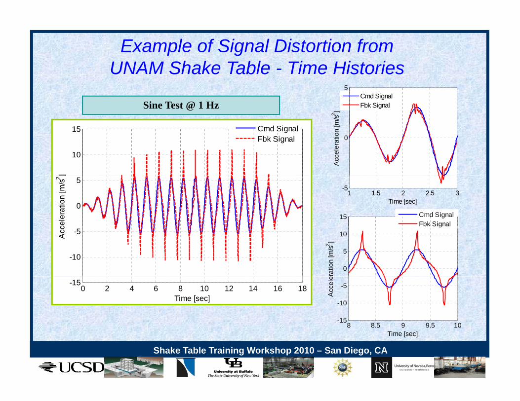
Example of Signal Distortion from UNAM Shake Table - Time HistoriesU S a e ab e e sto es
5
m/s2 ]
Cmd SignalFbk SignalSine Test @ 1 Hz
10
15
]
Cmd SignalFbk Signal 0
Acc
eler
atio
n [m
0
5
cele
ratio
n [m
/s2 ]
15 Cmd SignalFbk Signal
1 1.5 2 2.5 3-5
Time [sec]
-10
-5Acc
0
5
10
erat
ion
[m/s2 ]
Fbk Signal
0 2 4 6 8 10 12 14 16 18-15
Time [sec]
8 8.5 9 9.5 10-15
-10
-5
Acc
ele
Shake Table Training Workshop 2010 – San Diego, CA
8 8.5 9 9.5 10Time [sec]
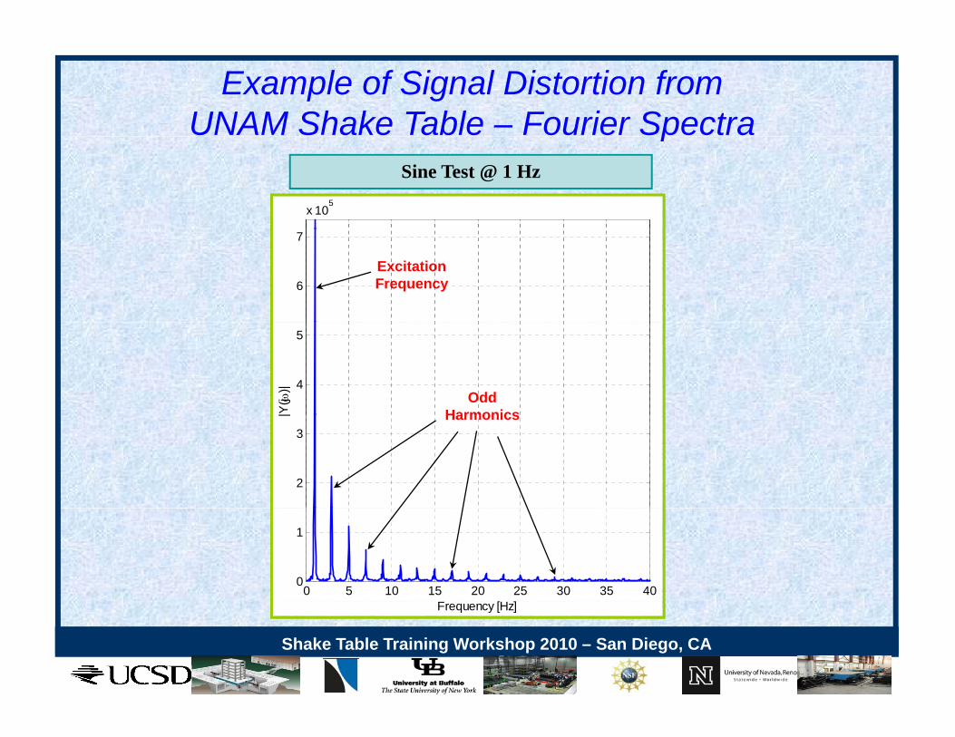
Example of Signal Distortion from UNAM Shake Table – Fourier Spectra
x 105
pSine Test @ 1 Hz
6
7
ExcitationFrequency
4
5
|Y(j
)| OddHarmonics
2
3
| Harmonics
0 5 10 15 20 25 30 35 400
1
Shake Table Training Workshop 2010 – San Diego, CA
Frequency [Hz]
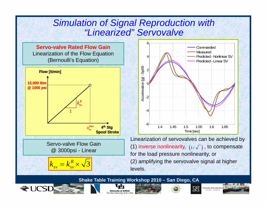
Simulation of Signal Reproduction with “Linearized” Servovalve
Servo-valve Rated Flow GainLinearization of the Flow Equation
(Bernoulli’s Equation)4
6
CommandedMeasuredPredicted - Nonlinear SVPredicted - Linear SV
Flow [lt/min]
10,000 lt/m@ 1000 psi
Flow [lt/min]
10,000 lt/m@ 1000 psi
0
2
ratio
n [g
] - S
p09
1
Rsvk
1
Rsvk
-4
-2
Acc
eler
4th StgSpool Stroke
maxsvx 4th Stg
Spool Strokemaxsvx
S l Fl G iLinearization of servovalves can be achieved by
1.4 1.45 1.5 1.55 1.6 1.65-6
Time [sec]
3Rsv svk k
Servo-valve Flow Gain @ 3000psi - Linear
(1) inverse nonlinearity, , to compensate for the load pressure nonlinearity, or (2) amplifying the servovalve signal at higher levels
1 /
Shake Table Training Workshop 2010 – San Diego, CA
sv sv levels.
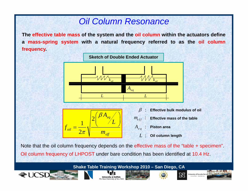
Oil Column ResonanceThe effective table mass of the system and the oil column within the actuators defineThe effective table mass of the system and the oil column within the actuators definea mass-spring system with a natural frequency referred to as the oil columnfrequency.
Sketch of Double Ended Actuator
oilk oilk
eqAL L
21
2
eq
oil
AL
fm
::e f fm
Effective bulk modulus of oil
Effective mass of the table
:e qA Piston area2 effm
:L Oil column length
Note that the oil column frequency depends on the effective mass of the “table + specimen”.Oil column frequency of LHPOST under bare condition has been identified at 10.4 Hz.
Shake Table Training Workshop 2010 – San Diego, CA
q y
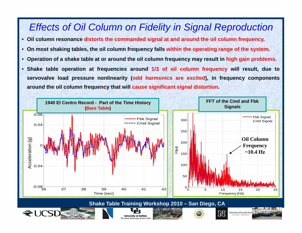
• Oil column resonance distorts the commanded signal at and around the oil column frequency.
Effects of Oil Column on Fidelity in Signal Reproduction
• On most shaking tables, the oil column frequency falls within the operating range of the system.
• Operation of a shake table at or around the oil column frequency may result in high gain problems.
• Shake table operation at frequencies around 1/3 of oil column frequency will result, due toservovalve load pressure nonlinearity (odd harmonics are excited), in frequency componentsaround the oil column frequency that will cause significant signal distortion.
1940 El Centro Record Part of the Time History FFT of the Cmd and Fbk
250
300Fbk SignalCmd Signal
0.04
0.06Fbk SignalCmd Signal
1940 El Centro Record - Part of the Time History (Bare Table)
FFT of the Cmd and Fbk Signals
150
200
250
|Y(j
)|0
Acc
eler
atio
n [g
]el
erat
ion
[g] Oil Column
Frequency~10.4 Hz
0 5 10 15 20 250
50
100
36 37 38 39 40 41 42-0.08
-0.04
AA
cce
Shake Table Training Workshop 2010 – San Diego, CA
0 5 10 15 20 25Frequency [Hz]
36 37 38 39 40 41 42Time [sec]
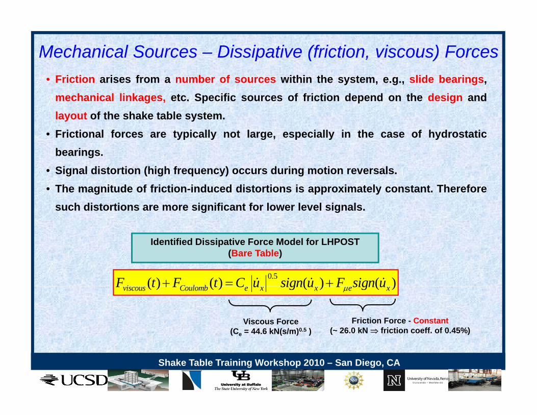
Mechanical Sources – Dissipative (friction, viscous) ForcesF i ti i f b f ithi th t lid b i• Friction arises from a number of sources within the system, e.g., slide bearings,mechanical linkages, etc. Specific sources of friction depend on the design andlayout of the shake table system.
• Frictional forces are typically not large, especially in the case of hydrostaticbearings.
• Signal distortion (high frequency) occurs during motion reversals.• The magnitude of friction-induced distortions is approximately constant. Therefore
such distortions are more significant for lower level signals.
Identified Dissipative Force Model for LHPOST (Bare Table)
0.5( ) ( ) ( ) ( )i C l bF t F t C u sign u F sign u ( ) ( ) ( ) ( )viscous Coulomb e x x e xF t F t C u sign u F sign u
Friction Force - Constant(~ 26.0 kN friction coeff. of 0.45%)
Viscous Force (Ce = 44.6 kN(s/m)0.5 )
Shake Table Training Workshop 2010 – San Diego, CA
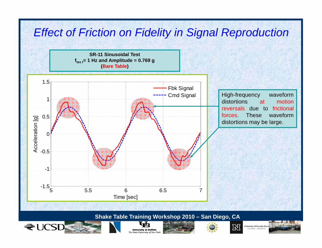
Effect of Friction on Fidelity in Signal Reproduction
SR-11 Sinusoidal Test ftes t= 1 Hz and Amplitude = 0.769 g
(Bare Table)
1
1.5Fbk SignalCmd Signal High-frequency waveform
distortions at motionreversals due to frictional
0
0.5
lera
tion
[g]
reversals due to frictionalforces. These waveformdistortions may be large.
-1
-0.5Acc
el
5 5.5 6 6.5 7-1.5
Time [sec]
Shake Table Training Workshop 2010 – San Diego, CA
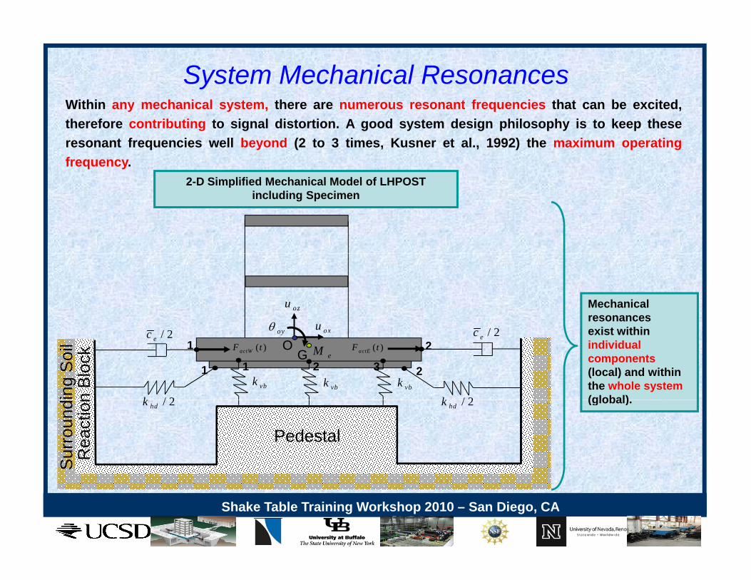
System Mechanical ResonancesWithin any mechanical system, there are numerous resonant frequencies that can be excited,Within any mechanical system, there are numerous resonant frequencies that can be excited,therefore contributing to signal distortion. A good system design philosophy is to keep theseresonant frequencies well beyond (2 to 3 times, Kusner et al., 1992) the maximum operatingfrequency.
2 D Simplified Mechanical Model of LHPOST2-D Simplified Mechanical Model of LHPOST including Specimen
Mechanical resonances
uozu
exist within individual components (local) and within the whole system (global)
Ooxuoy
n B
lock
/ 2ec / 2ec
/ 2k / 2kvbk vbk vbk
( )actWF t ( )actEF tG
1 2
1 2
21 3
ing
Soi
l
eM
(global).
Pedestal
Rea
ctio
n / 2hdk / 2hdk
Sur
roun
d
Shake Table Training Workshop 2010 – San Diego, CA
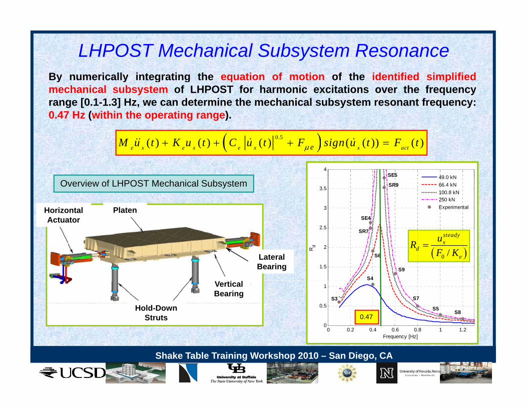
LHPOST Mechanical Subsystem ResonanceBy numerically integrating the equation of motion of the identified simplifiedBy numerically integrating the equation of motion of the identified simplifiedmechanical subsystem of LHPOST for harmonic excitations over the frequencyrange [0.1-1.3] Hz, we can determine the mechanical subsystem resonant frequency:0.47 Hz (within the operating range).
0.5( ) ( ) ( ) ( ( )) ( )e x e x e x x acteM u t K u t C u t F sign u t F t
449 0 kNSE5
Overview of LHPOST Mechanical Subsystem
PlatenHorizontal Actuator
2.5
3
3.5
49.0 kN66.4 kN100.8 kN250 kNExperimental
SR9
SE4
S
Lateral Bearing 1.5
2
5
Rd
S9
SR7
S4
S6 0 /
steadyx
de
uRF K
Vertical Bearing
Hold-Down Struts
0 0.2 0.4 0.6 0.8 1 1.20
0.5
1
S5 S8
S7S3
0.47
Shake Table Training Workshop 2010 – San Diego, CA
Frequency [Hz]
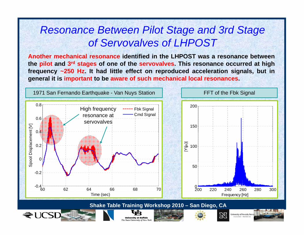
Resonance Between Pilot Stage and 3rd Stageof Servovalves of LHPOSTof Servovalves of LHPOST
Another mechanical resonance identified in the LHPOST was a resonance betweenthe pilot and 3rd stages of one of the servovalves. This resonance occurred at highfrequency ~250 Hz. It had little effect on reproduced acceleration signals, but infrequency 250 Hz. It had little effect on reproduced acceleration signals, but ingeneral it is important to be aware of such mechanical local resonances.
1971 San Fernando Earthquake - Van Nuys Station FFT of the Fbk Signal
150
200
0 4
0.6
0.8
nt [V
]
Fbk SignalCmd Signal
High frequencyresonance atservovalves
100
|Y(j
)|
0
0.2
0.4
ool D
ispl
acem
en
200 220 240 260 280 3000
50
60 62 64 66 68 70-0.4
-0.2
Sp
Shake Table Training Workshop 2010 – San Diego, CA
Frequency [Hz]Time (sec)
Shake Table – Specimen Interaction• A more difficult source of signal distortion to compensate for is due to specimen
compliance and resulting table - specimen interaction. The reasons are:
Location of the specimen on the platen (e.g., eccentricity-induced torsional motion
of the table-specimen system) will contribute to cross coupling of actuator axes.
M t d i h i i ti t t t l b h i ll b d Most dynamic research on specimens investigates structural behavior well beyond
the elastic range of materials. Therefore, the overall system (table + specimen)
dynamics changes as the specimen enters the plastic range.
In general, shake table tuning is based on the assumption of a fixed (specimen)
coupled mass, since this determines the oil column frequency. With a yielding and
degrading specimen, the oil column frequency is load dependent and time-varying.
Shake Table Training Workshop 2010 – San Diego, CA
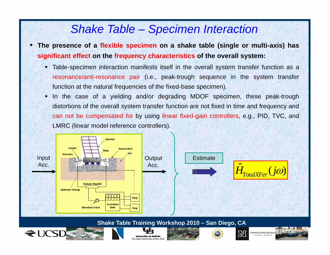
Shake Table – Specimen Interaction• The presence of a flexible specimen on a shake table (single or multi-axis) hasThe presence of a flexible specimen on a shake table (single or multi axis) has
significant effect on the frequency characteristics of the overall system: Table-specimen interaction manifests itself in the overall system transfer function as a
resonance/anti-resonance pair (i.e., peak-trough sequence in the system transferp ( , p g q yfunction at the natural frequencies of the fixed-base specimen).
In the case of a yielding and/or degrading MDOF specimen, these peak-troughdistortions of the overall system transfer function are not fixed in time and frequency andcan not be compensated for by using linear fixed-gain controllers, e.g., PID, TVC, andLMRC (linear model reference controllers).
SpecimenSpecimen
Reaction block
SoilPlaten
Actuator
Servovalve
Reaction block
SoilPlaten
Actuator
Servovalve
InputAcc.
OutputAcc. ˆ ( )TotalXFerH j
Estimate
Accumulator Banks
Pump
Pump
Hydraulic Manifold
Blowndown Valves
Hydrostatic bearings
Accumulator Banks
Pump
Pump
Hydraulic Manifold
Blowndown Valves
Hydrostatic bearings
( )TotalXFer j
Shake Table Training Workshop 2010 – San Diego, CA
Banks PumpBlowndown Valves Banks PumpBlowndown Valves
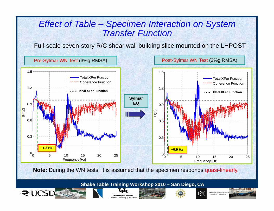
Effect of Table – Specimen Interaction on System Transfer Function
Pre-Sylmar WN Test (3%g RMSA) Post-Sylmar WN Test (3%g RMSA)
Full-scale seven-story R/C shear wall building slice mounted on the LHPOST
1.2
1.5
Total XFer FunctionCoherence Function
Ideal XFer Function1.2
1.5
Total XFer FunctionCoherence Function
Ideal XFer Function
0.9
|H(j
)|
Sylmar EQ 0.9
|H(j
)|
Ideal XFer Function
0.3
0.6
0.3
0.6
Note: During the WN tests, it is assumed that the specimen responds quasi-linearly.
0 5 10 15 20 250
Frequency [Hz]
~1.3 Hz
0 5 10 15 20 250
Frequency [Hz]
~0.9 Hz
Shake Table Training Workshop 2010 – San Diego, CA
g , p p q y
Some Options for “Dealing” with the Effects ofgTable-Specimen Interaction
• Iteratively match the reference (commanded) earthquake record applied at
full-scale without the specimen on the table, then mount the specimen,
and test it with the last iterative earthquake input file.
Drawback: Additional error in earthquake signal reproduction will be
introduced by specimen-table interaction. Unless the specimen is very light
relative to the table platform, signal distortions will be significant.
Shake Table Training Workshop 2010 – San Diego, CA

Some Options for “Dealing” with the Effects ofTable Specimen Interaction
• Iteratively match the reference (commanded) earthquake record scaled
Table-Specimen Interaction
down in amplitude with the specimen on the table, then scale up the drive
signal (from the last iteration) for the actual test. Errors in signal
reproduction resulting from this process are likely to be less severe thanreproduction resulting from this process are likely to be less severe than
in the previous approach.
Drawback: Additional error in signal reproduction will be introduced by the Drawback: Additional error in signal reproduction will be introduced by the
fact that the specimen is behaving quasi-linearly during the signal matching
procedure, but not during the actual test, and further errors will be caused
by non-scalable nonlinearities in the table response itself. Also, the risk of
prematurely damaging the specimen is high.
Shake Table Training Workshop 2010 – San Diego, CA

Signal Distortion Compensation Techniques
MTS 469D Seismic Controller
SYSTEMLINEARITY
PROGRAM
LINEAR NONLINEAR
PROGRAMSHAPE
Used for iteratively matching the reference (commanded)
Amplitude PhaseControl(APC)
AdaptiveHarmonic
Cancellation(AHC)
SINUSOIDAL
the reference (commanded) time history
Iterative techniques can not
Adaptive Online
qcompletely remove the effects of table-specimen interaction. Real time nonlinear adaptive controlInverse
Control(AIC)
Iteration(OLI)
NON-SINUSOIDAL nonlinear adaptive control techniques are required to control evolving nonlinear interaction.
Shake Table Training Workshop 2010 – San Diego, CA

OnLine Iteration (OLI) Technique
Response RMS error versus OLI iteration number for Sylmar record at 0.852-g calibration PGA lit d th d d i fil i h d t th th it ti
Shake Table Training Workshop 2010 – San Diego, CA
PGA amplitude, the converged drive file is reached at the seventh iteration.
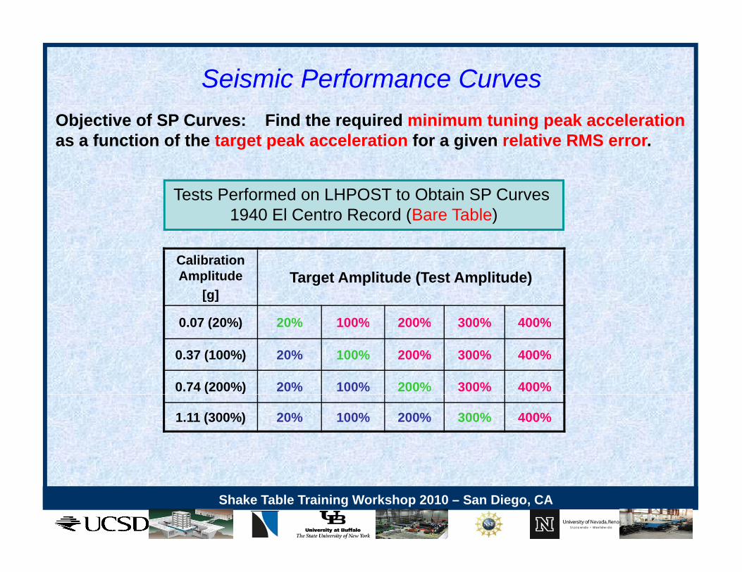
Seismic Performance CurvesObjective of SP Curves: Find the required minimum tuning peak accelerationas a function of the target peak acceleration for a given relative RMS error.
Tests Performed on LHPOST to Obtain SP Curves 1940 El Centro Record (Bare Table)
Calibration Amplitude
[g]Target Amplitude (Test Amplitude)
0 07 (20%) 20% 100% 200% 300% 400%0.07 (20%) 20% 100% 200% 300% 400%
0.37 (100%) 20% 100% 200% 300% 400%
0.74 (200%) 20% 100% 200% 300% 400%
1.11 (300%) 20% 100% 200% 300% 400%
Shake Table Training Workshop 2010 – San Diego, CA
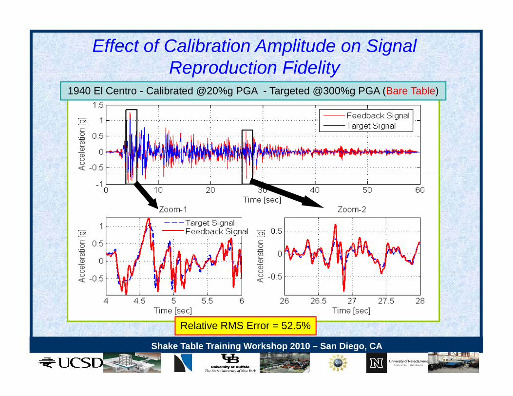
Effect of Calibration Amplitude on Signal Reproduction Fidelity
1940 El Centro - Calibrated @20%g PGA - Targeted @300%g PGA (Bare Table)
Reproduction Fidelity
R l ti RMS E 52 5%
Shake Table Training Workshop 2010 – San Diego, CA
Relative RMS Error = 52.5%
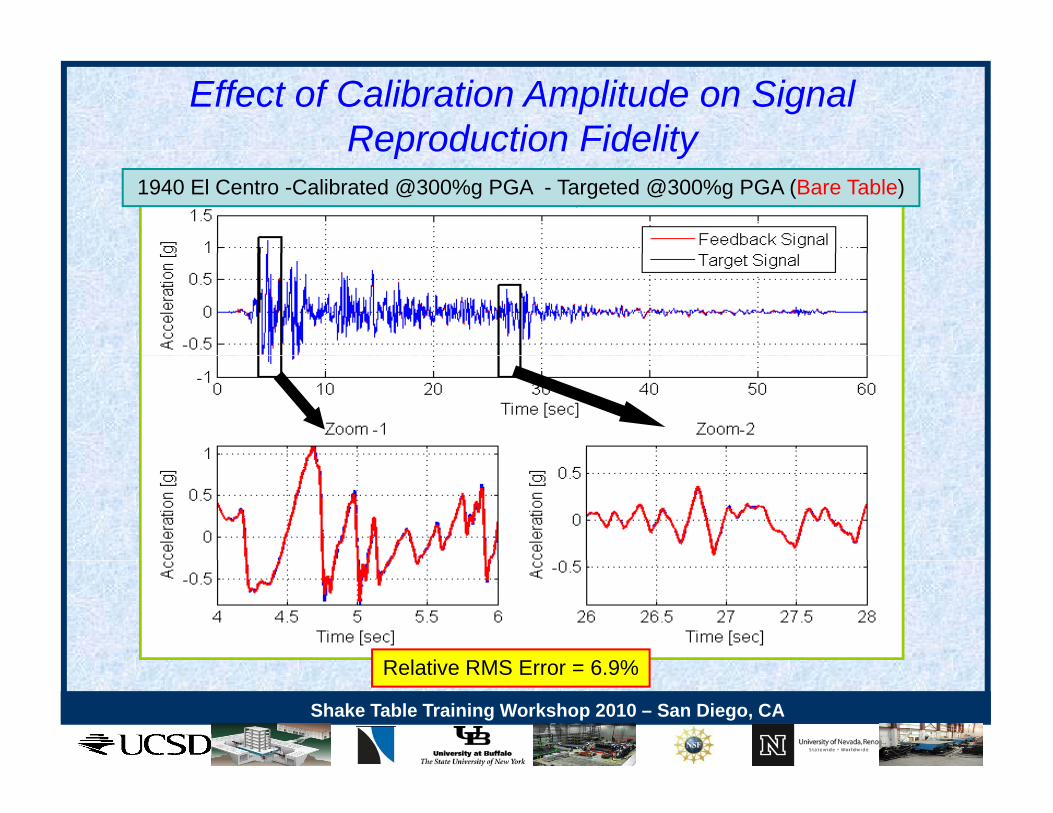
Effect of Calibration Amplitude on Signal Reproduction Fidelity
1940 El Centro -Calibrated @300%g PGA - Targeted @300%g PGA (Bare Table)
Reproduction Fidelity
R l ti RMS E 6 9%
Shake Table Training Workshop 2010 – San Diego, CA
Relative RMS Error = 6.9%
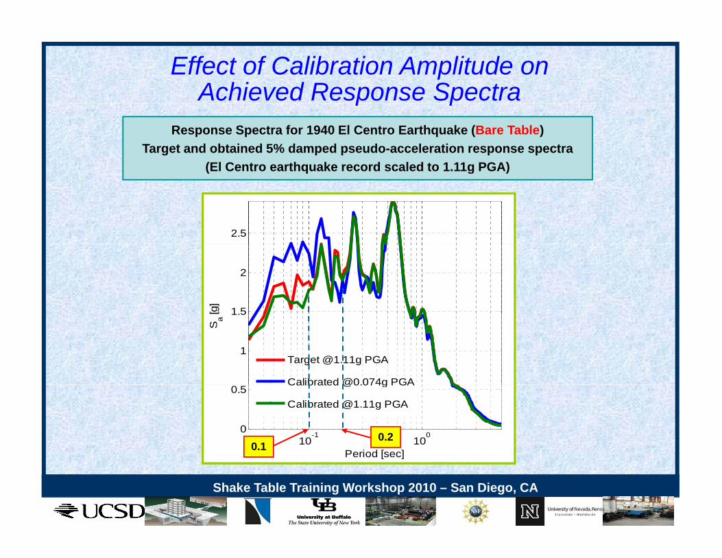
Effect of Calibration Amplitude onAchieved Response Spectrap p
Response Spectra for 1940 El Centro Earthquake (Bare Table)Target and obtained 5% damped pseudo-acceleration response spectra
(El Centro earthquake record scaled to 1.11g PGA) ( q g )
2.5
1.5
2
[g]
1
1.5
Sa
Target @1.11g PGA
Calibrated @0.074g PGA
10-1
100
0
0.5
Period [sec]
Calibrated @0.074g PGA
Calibrated @1.11g PGA
0.10.2
Shake Table Training Workshop 2010 – San Diego, CA
Period [sec]
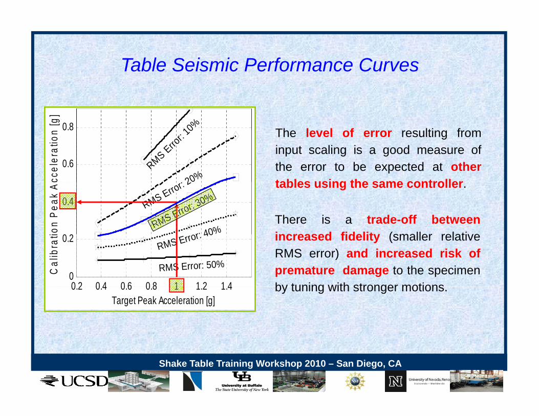
Table Seismic Performance Curves
Th l l f lti f0.8 [g]
10%0.8 [g]
10%The level of error resulting frominput scaling is a good measure ofthe error to be expected at othertables using the same controller
0.6
0.8
ccel
erat
ion
RMS Error: 1
0
20%0.6
0.8
ccel
erat
ion
RMS Error: 1
0
20% tables using the same controller.
There is a trade-off betweenincreased fidelity (smaller relative0 2
0.4
on P
eak
Ac
RMS Error: 20
RMS Error: 30%
or: 40%0 2
0.4
on P
eak
Ac
RMS Error: 20
RMS Error: 30%
or: 40% increased fidelity (smaller relativeRMS error) and increased risk ofpremature damage to the specimenby tuning with stronger motions0 2 0 4 0 6 0 8 1 1 2 1 4
0
0.2
Cal
ibra
ti
RMS Error: 40%
RMS Error: 50%
0 2 0 4 0 6 0 8 1 1 2 1 40
0.2
Cal
ibra
ti
RMS Error: 40%
RMS Error: 50%
by tuning with stronger motions.0.2 0.4 0.6 0.8 1 1.2 1.4Target Peak Acceleration [g]
0.2 0.4 0.6 0.8 1 1.2 1.4Target Peak Acceleration [g]
Shake Table Training Workshop 2010 – San Diego, CA

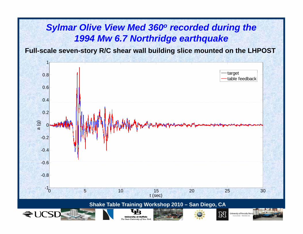
Sylmar Olive View Med 360o recorded during the 1994 Mw 6.7 Northridge earthquake
1
target
g qFull-scale seven-story R/C shear wall building slice mounted on the LHPOST
0.4
0.6
0.8 targettable feedback
0
0.2
a (g
)
0 6
-0.4
-0.2
0 5 10 15 20 25 30-1
-0.8
-0.6
Shake Table Training Workshop 2010 – San Diego, CA
0 5 10 15 20 25 30t (sec)
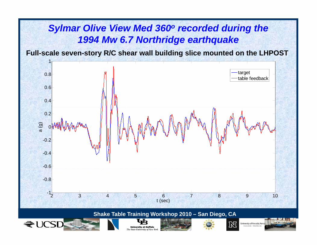
Sylmar Olive View Med 360o recorded during the 1994 Mw 6.7 Northridge earthquake
0.8
1
target
Full-scale seven-story R/C shear wall building slice mounted on the LHPOST
0.4
0.6
table feedback
0
0.2
a (g
)
-0.6
-0.4
-0.2
2 3 4 5 6 7 8 9 10-1
-0.8
t (sec)
Shake Table Training Workshop 2010 – San Diego, CA
t (sec)
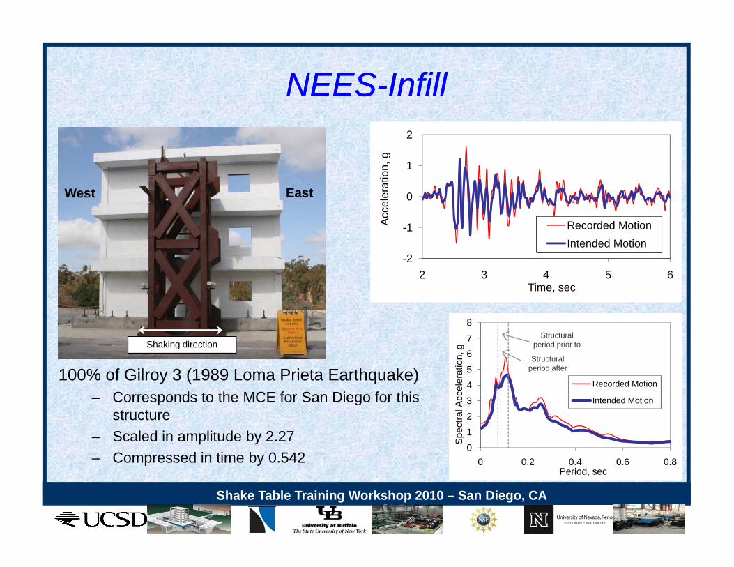
NEESNEES--InfillInfill
1
2
on, g
EastWest
-1
0
Acc
eler
atio
Recorded MotionIntended Motion
-22 3 4 5 6
Time, sec
8
100% of Gilroy 3 (1989 Loma Prieta Earthquake)
Shaking direction
45678
eler
atio
n, g
Recorded Motion
Structural period prior to
Structural period after
– Corresponds to the MCE for San Diego for this structure
– Scaled in amplitude by 2.27– Compressed in time by 0.542
0123
0 0 2 0 4 0 6 0 8S
pect
ral A
cc Intended Motion
Shake Table Training Workshop 2010 – San Diego, CA
Compressed in time by 0.542 0 0.2 0.4 0.6 0.8Period, sec

References on Design, Analysis, Characterization, and Modeling of LHPOSTand Modeling of LHPOST
Van Den Einde, L., Restrepo, J., Conte, J. P., Luco, E., Seible, F., Filiatrault, A., Clark, A.,Johnson, A., Gram, M., Kusner, D., and Thoen, B., “Development of the George E. BrownJr. Network for Earthquake Engineering Simulation (NEES) Large High PerformanceOut door Shake Table at the University of California San Diego ” Proc of 13 th WorldOut-door Shake Table at the University of California, San Diego,” Proc. of 13-th WorldConfer-ence on Earthquake Engineering, Vancouver, BC Canada, August 1-6, 2004,Paper No. 3281.
Ozcelik, O., Conte, J. P., and Luco, J. E., “Virtual Model of the UCSD-NEES HighPerfor-mance Outdoor Shake Table,” Proc. of the Fourth World Conference on StructuralControl and Monitoring, San Diego, California, July 11-13, 2006.
Ozcelik, O., Luco, J. E., and Conte, J. P., “Identification of the Mechanical Subsystem of theNEES-UCSD Shake Table by a Least-Squares Approach,” Journal of EngineeringS UCS S a e ab e by a eas Squa es pp oac , Jou a o g ee gMechanics, ASCE, Vol. 134, No. 1, pp. 23-34, 2008.
Ozcelik, O., Luco, J. E., Conte, J. P., Trombetti, T. L., and Restrepo, J., “ExperimentalCharacterization, Modeling and Identification of the NEES-UCSD Shake Table MechanicalSystem ” Earthquake Engineering and Structural Dynamics Vol 37 Issue 2 pp 243 264System, Earthquake Engineering and Structural Dynamics, Vol. 37, Issue 2, pp. 243-264,2008.
Luco, J. E., Ozcelik, O., and Conte, J. P., “Acceleration Tracking Performance of the NEES-UCSD Shake Table,” Journal of Structural Engineering, ASCE, Vol. 136, No. 5, pp. 481-490 2010
Shake Table Training Workshop 2010 – San Diego, CA
490, 2010.

Questions?Questions?
Shake Table Training Workshop 2010 – San Diego, CA
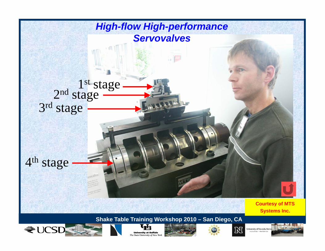
High-flow High-performanceServovalves
3rd stage2nd stage
1st stage
3 stage
4th stage
Courtesy of MTS
Shake Table Training Workshop 2010 – San Diego, CA
Courtesy of MTSSystems Inc.

Shake Table Training Workshop 2010 – San Diego, CA

ThreeThree--Variable Controller (TVC)Variable Controller (TVC)Control ModeControl Mode
Reference
(DisplacementVelocity, Acceleration)
10/Dmax PFk
FeedforwardGains
refx
refx
Reference
(DisplacementVelocity, Acceleration)
10/Dmax PFk
FeedforwardGains
refx
refx
ReferenceSignal
+
+++
10/Vmax
10/Amax AFk
ref
refx
refx
VFk
Ref
eren
ce
Gen
erat
orReference
Signal
+
+++
10/Vmax
10/Amax AFk
ref
refx
refx
VFk
Ref
eren
ce
Gen
erat
or
DisplacementFbk
+- +
++-+
10/Amax
10/Dmax
Notch Filter
Qty = 5
JFk
Pk MkFeedback
Gains
MasterGain
ref
fbkx
Controller Output
to Servovalves
ck
or
DisplacementFbk
+- +
++-+
10/Amax
10/Dmax
Notch Filter
Qty = 5
JFk
Pk MkFeedback
Gains
MasterGain
ref
fbkx
Controller Output
to Servovalves
ck
or
AccelerationFbk
++
+10/Vmax
10/Amax
Notch Filter
Ak
Vk Ik 1/ s
Reset Integrator
fbkx
fbkx
F
Feed
bac
Gen
erat
o
AccelerationFbk
++
+10/Vmax
10/Amax
Notch Filter
Ak
Vk Ik 1/ s
Reset Integrator
fbkx
fbkx
F
Feed
bac
Gen
erat
o
ForceFbk
Lowpass Filter
10/Fmax
Highpass Filter
DPkfbkFForceFbk
Lowpass Filter
10/Fmax
Highpass Filter
DPkfbkF
TVC is a displacement controller with sophisticated feed-forward gains.
Courtesy of MTSSystems Inc.
Shake Table Training Workshop 2010 – San Diego, CA
TVC is a displacement controller with sophisticated feed forward gains.
Some Options for “Dealing” with the Effects ofTable-Specimen Interaction
• Mount the specimen on the table, but restrain it as much as possible so
that it can not move relative to the table platform (accomplished by
Table-Specimen Interaction
that it can not move relative to the table platform (accomplished by
adding extra bracing, etc.), and iteratively match the reference
(commanded) time history applied at full scale. The benefit of this( ) y
approach is that the overturning moment due to the high center of gravity
of the specimen is compensated for in the signal matching procedure.
Drawback: It may be unacceptable to run several pre-tests as some
degradation of the model may occur. The shaking table user must
therefore make a judgement as to whether the accuracy of table motion is
more important than the integrity of the specimen for the final test(s).
Shake Table Training Workshop 2010 – San Diego, CA

NEESNEES--InfillInfill
1
2
on, g
EastWest
-1
0
Acc
eler
atio
Recorded MotionIntended Motion
-22 3 4 5 6
Time, sec
8
100% of Gilroy 3 (1989 Loma Prieta Earthquake)
Shaking direction
45678
eler
atio
n, g
Recorded Motion
Structural period prior to
Structural period after
– Corresponds to the MCE for San Diego for this structure
– Scaled in amplitude by 2.27– Compressed in time by 0.542
0123
0 0 2 0 4 0 6 0 8S
pect
ral A
cc Intended Motion
Shake Table Training Workshop 2010 – San Diego, CA
Compressed in time by 0.542 0 0.2 0.4 0.6 0.8Period, sec
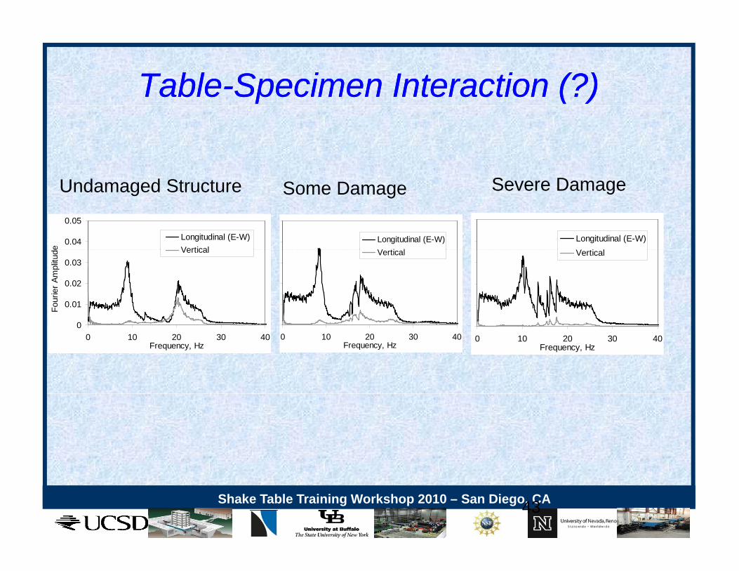
TableTable--Specimen Interaction (?)Specimen Interaction (?)
S D
0.04
0.05
e
Longitudinal (E-W)Vertical
Longitudinal (E-W)V ti l
Longitudinal (E-W)V ti l
Undamaged Structure Some Damage Severe Damage
0.01
0.02
0.03
Four
ier A
mpl
itude Vertical Vertical Vertical
00 10 20 30 40
Frequency, Hz0 10 20 30 40
Frequency, Hz0 10 20 30 40
Frequency, Hz
Shake Table Training Workshop 2010 – San Diego, CA43
Sylmar Olive View Med 360o recorded during the 1994 Mw 6.7 Northridge earthquake
1
target
g qFull-scale seven-story R/C shear wall building slice mounted on the LHPOST
0.4
0.6
0.8 targettable feedback
0
0.2
a (g
)
0 6
-0.4
-0.2
0 5 10 15 20 25 30-1
-0.8
-0.6
Shake Table Training Workshop 2010 – San Diego, CA
0 5 10 15 20 25 30t (sec)

Sylmar Olive View Med 360o recorded during the 1994 Mw 6.7 Northridge earthquake
0.8
1
target
Full-scale seven-story R/C shear wall building slice mounted on the LHPOST
0.4
0.6
table feedback
0
0.2
a (g
)
-0.6
-0.4
-0.2
2 3 4 5 6 7 8 9 10-1
-0.8
t (sec)
Shake Table Training Workshop 2010 – San Diego, CA
t (sec)
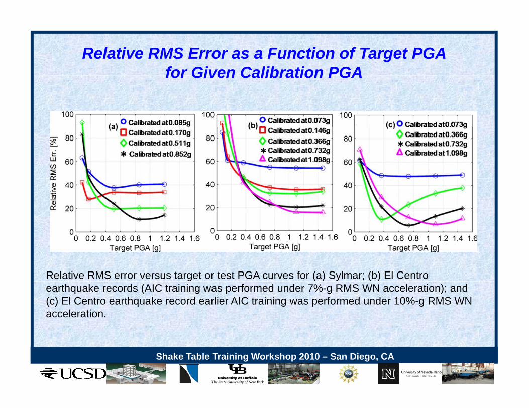
Relative RMS Error as a Function of Target PGA for Given Calibration PGAfor Given Calibration PGA
Relative RMS error versus target or test PGA curves for (a) Sylmar; (b) El Centro earthquake records (AIC training was performed under 7%-g RMS WN acceleration); and (c) El Centro earthquake record earlier AIC training was performed under 10%-g RMS WN acceleration.
Shake Table Training Workshop 2010 – San Diego, CA
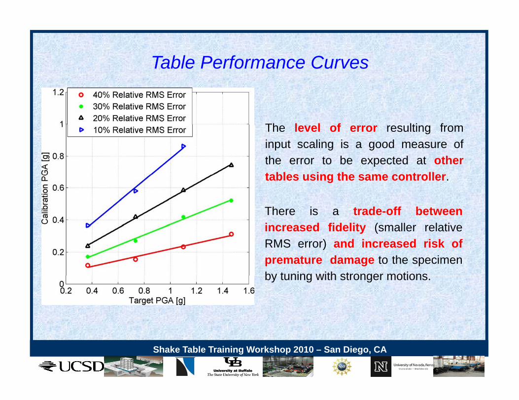
Table Performance Curves
Th l l f lti fThe level of error resulting frominput scaling is a good measure ofthe error to be expected at othertables using the same controllertables using the same controller.
There is a trade-off betweenincreased fidelity (smaller relativeincreased fidelity (smaller relativeRMS error) and increased risk ofpremature damage to the specimenby tuning with stronger motionsby tuning with stronger motions.
Shake Table Training Workshop 2010 – San Diego, CA

LHPOST Performance Specifications
• Size: 12.2 m x 7.6 m• Vertical Payload: 20 MNy• Frequency Bandwidth: 0-20 Hz• Phase 1: Uniaxial System:
– Stroke: 0.75 m; Velocity: 1.8 m/sec; Acceleration: 3.0g• Phase 2: Triaxial System:
Direction Acceleration Velocity Displacement Horizontal-X g3 m/s1.8 m0.75 Horizontal-Y g1.5 m/s0.9 m0.375
V i l 1 0 /0 0 1 0Vertical g1.0 m/s0.5 m0.150
Shake Table Training Workshop 2010 – San Diego, CA
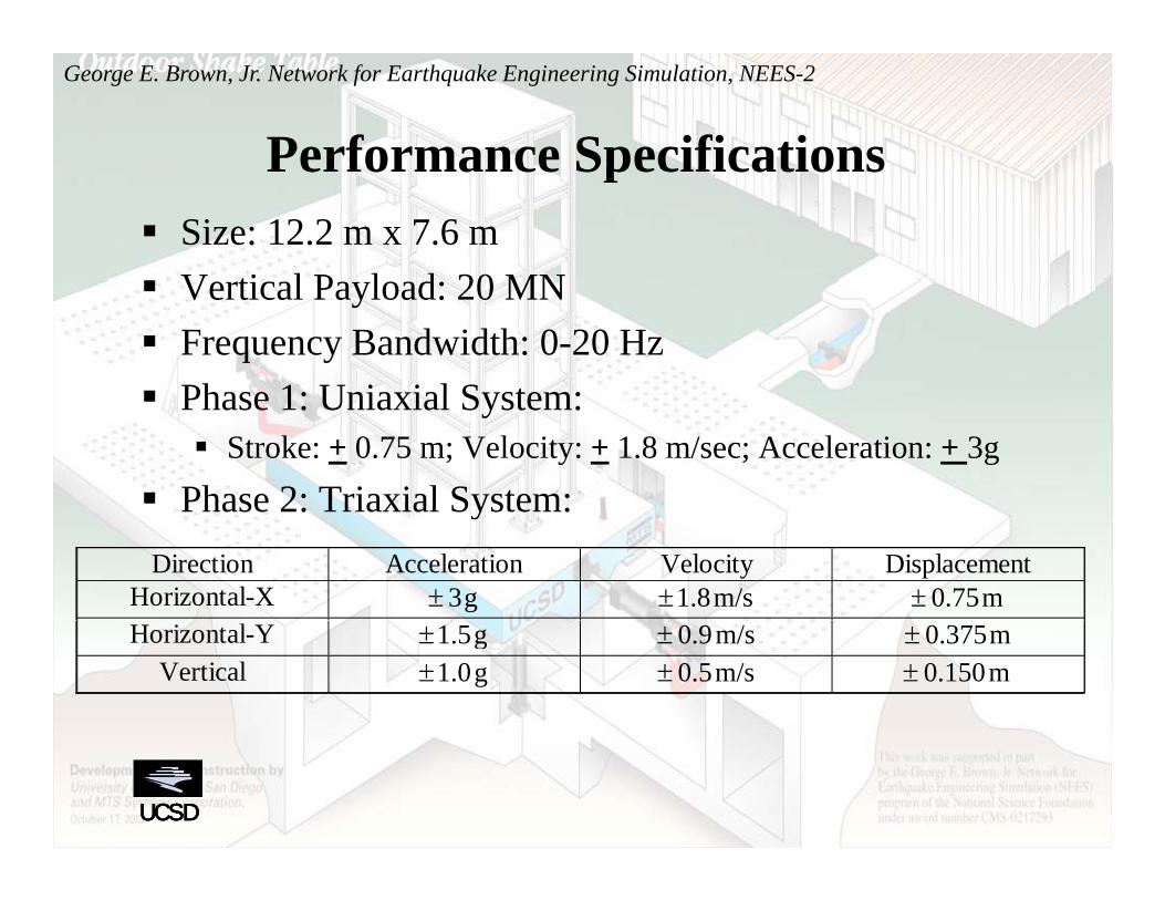
George E. Brown, Jr. Network for Earthquake Engineering Simulation, NEES-2
Performance SpecificationsPerformance Specifications Size: 12.2 m x 7.6 m
V ti l P l d 20 MN Vertical Payload: 20 MN Frequency Bandwidth: 0-20 Hz Phase 1: Uniaxial System: Phase 1: Uniaxial System: Stroke: + 0.75 m; Velocity: + 1.8 m/sec; Acceleration: + 3g
Phase 2: Triaxial System:Phase 2: Triaxial System:Direction Acceleration Velocity Displacement
Horizontal-X g3 m/s1.8 m0.75 Horizontal-Y g1.5 m/s0.9 m0.375
Vertical g1.0 m/s0.5 m0.150
UCSDUCSD