SGN: Sequential Grouping Networks for Instance Segmentation

Shu Liu† Jiaya Jia†,[ Sanja Fidler‡ Raquel Urtasun§,‡

†The Chinese University of Hong Kong [Youtu Lab, Tencent§Uber Advanced Technologies Group ‡University of Toronto

{sliu, leojia}@cse.cuhk.edu.hk {fidler, urtasun}@cs.toronto.edu

Abstract

In this paper, we propose Sequential Grouping Net-

works (SGN) to tackle the problem of object instance seg-

mentation. SGNs employ a sequence of neural networks,

each solving a sub-grouping problem of increasing seman-

tic complexity in order to gradually compose objects out

of pixels. In particular, the first network aims to group

pixels along each image row and column by predicting

horizontal and vertical object breakpoints. These break-

points are then used to create line segments. By exploit-

ing two-directional information, the second network groups

horizontal and vertical lines into connected components.

Finally, the third network groups the connected compo-

nents into object instances. Our experiments show that our

SGN significantly outperforms state-of-the-art approaches

in both, the Cityscapes dataset as well as PASCAL VOC.

1. Introduction

The community has achieved remarkable progress for

tasks such as object detection [32, 10] and semantic seg-

mentation [27, 6] in recent years. Research along these lines

opens the door to challenging life-changing tasks, including

autonomous driving and personalized robotics.

Instance segmentation is a task that jointly considers ob-

ject detection and semantic segmentation, by aiming to pre-

dict a pixel-wise mask for each object in an image. The

problem is inherently combinatorial, requiring us to group

sets of pixels into coherent components. Occlusion and

vastly varying number of objects across scenes further in-

crease the complexity of the task. In street scenes, such as

those in the Cityscapes dataset [7], current methods merely

reach 20% accuracy in terms of average precision, which is

still far from satisfactory.

Most of the instance segmentation approaches employ a

two-step process by treating the problem as a foreground-

background pixel labeling task within the object detection

boxes [15, 16, 1, 29, 30]. Instead of labeling pixels, [4] pre-

dicts a polygon outlining the object instance using a Recur-

rent Neural Network (RNN). In [41, 40], large patches are

exhaustively extracted from an image and a Convolutional

Neural Network (CNN) is trained to predict instance la-

bels inside each patch. A dense Conditional Random Field

(CRF) is then used to get consistent labeling of the full im-

age. In [33, 31], an RNN is used to produce one object mask

per time step. The latter approaches face difficulties on im-

ages of street scenes which contain many objects. More re-

cently, [3] learned a convolutional net to predict the energy

of the watershed transform. Its complexity does not depend

on the number of objects in the scene.

In this paper, we break the task of object instance seg-

mentation into several sub-tasks that are easier to tackle.

We propose a grouping approach that employs a sequence

of neural networks to gradually compose objects from sim-

pler constituents. In particular, the first network aims to

group pixels along each image row and column by predict-

ing horizontal and vertical object breakpoints. These are

then used to create horizontal and vertical line segments.

The second neural network groups these line segments into

connected components. The last network merges compo-

nents into coherent object instances, thus solving the prob-

lem of object splitting due to occlusion. Due to its sequen-

tial nature, we call our approach Sequential Grouping Net-

works (SGN). We evaluate our method on the challenging

Cityscapes dataset. SGN significantly outperforms state-of-

the-art, achieving a 5% absolute and 25% relative boost in

accuracy. We also improve over state-of-the-art on PAS-

CAL VOC for general object instance segmentation which

further showcases the strengths of our proposed approach.

2. Related Work

The pioneering work of instance segmentation [15, 8]

aimed at both classifying object proposals as well as la-

beling an object within each box. In [29, 30], high-

quality mask proposals were generated using CNNs. Simi-

larly, MNC [9] designed an end-to-end trainable multi-task

network cascade to unify bounding box proposal genera-

tion, pixel-wise mask proposal generation and classifica-

13496

horizontal breakpoint map horizontal line segments

vertical breakpoint map vertical line segments

LineNet MergerNet

input image instance

segmentationcomponents

Figure 1. Sequential Grouping Networks (SGN): We first predict breakpoints. LineNet groups them into connected components, which

are finally composed by the MergerNet to form our final instances.

tion. SAIS [16] improved MNC by learning to predict dis-

tances to instance boundaries, which are then decoded into

high-quality masks by a set of convolution operations. A

recursive process was proposed in [22] to iteratively refine

the predicted pixel-wise masks. Recently, [4] proposed to

predict polygons outlining each object instance which has

the advantage of efficiently capturing object shape.

MPA [26] modeled objects as composed of generic parts,

which are predicted in a sliding window fashion and then

aggregated to produce instances. IIS [20] is an iterative ap-

proach to refine the instance masks. In [21], the authors

utilized a fully convolutional network by learning to com-

bine different relative parts into an instance. Methods of

[41, 40] extracted patches from the image and used a CNN

to directly infer instance IDs inside each patch. A CRF is

then used to derive globally consistent labels of the image.

In [1, 2], a CRF is used to assign each pixel to an object

detection box by exploiting semantic segmentation maps.

Similarly, PFN [23] utilized semantic segmentation to pre-

dict the bounding box each pixel belongs to. Pixels are then

grouped into clusters based on the distances to the predicted

bounding boxes. In [36], the authors predict the direction to

the instance’s center for each pixel, and exploits templates

to infer the location of instances on the predicted angle map.

Recently, Bai and Urtasun [3] utilized a CNN to learn an

energy of the watershed transform. Instances naturally cor-

respond to basins in the energy map. It avoids the combina-

torial complexity of instance segmentation. In [18], seman-

tic segmentation and object boundary prediction were ex-

ploited to separate instances. Different types of label trans-

formation were investigated in [17]. Pixel association was

learned in [28] to differentiate between instances.

Finally, RNN [33, 31] was used to predict an object label

at each time step. However, since RNNs typically do not

perform well when the number of time steps is large, these

methods have difficulties in scaling up to the challenging

multi-object street scenes.

Here, we propose a new type of approach to instance

segmentation by exploiting several neural networks in a se-

quential manner, each solving a sub-grouping problem.

3. Sequential Grouping Networks

In this section, we present our approach to object in-

stance segmentation. Following [3, 18], we utilize seman-

tic segmentation to identify foreground pixels, and restrict

our reasoning to them. We regard instances as composed of

breakpoints that form line segments, which are then com-

bined to generate full instances. Fig. 1 illustrates our model.

We first introduce the network to identify breakpoints, and

show how to use them to group pixels into lines in Sub-

sec. 3.2. In Subsec. 3.3, we propose a network that groups

lines into components, and finally the network to group

components into instances is introduced in Subsec. 3.4.

3.1. Predicting Breakpoints

Our most basic primitives are defined as the pixel loca-

tions of breakpoints, which, for a given direction, represent

the beginning or end of each object instance. Note that we

reason about the breakpoints in both the horizontal and ver-

tical direction. For the horizontal direction, computing the

starting points amounts to scanning the image from left to

right, one row at a time, recording the change points where

a new instance appears. For the vertical direction, the same

process is conducted from top to bottom. As a consequence,

the boundary between instances is considered as a starting

point. The termination points are then the pixels where an

instance has a boundary with the background. Note that

this is different from predicting standard boundaries as it

additionally encodes the direction where the interior of the

instance is.

We empirically found that introducing two additional

labels encoding the instance interior as well as the back-

ground is helpful to make the end-point prediction sharper.

Each pixel in an image is thus labeled with 4 labels encod-

ing either background, interior, starting point or a termina-

tion point. We refer the reader to Fig. 1 for an example.

Network Structure We exploit a CNN to perform this

pixel-wise labeling task. The network takes the original im-

age as input and predicts two label maps, one per direction

as shown in Fig. 2(a). Our network is based on Deeplab-

3497

(a) (b)

Figure 2. Illustration of (a) network structure for predicting breakpoints, and (b) the fusion operation.

(a) (b)decoding direction

Figure 3. Line decoding process. Green and red points are start-

ing and termination ones. Scanning from left to right, there is no

more line segment in the area pointed by the black arrow in (a)

due to erroneous point detection. The reversal scanning in (b) gets

new line hypothesis in this area, shown by orange line segments.

LargeFOV [5]. We use a modified VGG16 [35], and make

it fully convolutional as in FCN [27]. To preserve precise

localization information, we remove pool4 and pool5 lay-

ers. To enlarge the receptive field, we make use of dilated

convolutions [39, 6] in the conv5 and conv6 layers.

Similar to the methods in [30, 24, 12], we augment the

network by connecting lower layers to higher ones in order

to capture fine details. In particular, we fuse information

from conv5 3, conv4 3 and conv3 3 layers, as shown in Fig.

2 (b). To be more specific, we first independently filter the

input feature maps through 128 filters of size 3 × 3, which

are then concatenated. We then utilize another set of 128

filters of size 3× 3 to decrease the feature dimension. After

fusion with conv3 3, the feature map is downscaled by a

factor of 4. Predictions for breakpoint maps are then made

by two independent branches on top of it.

Learning Predicting breakpoints is hard since they are

very sparse, making the distribution of labels unbalanced

and dominated by the background and interior pixels. To

mitigate this effect, similar to HED [38], we re-weight the

cross-entropy loss based on inverse of the frequency of each

class in the mini-batch.

3.2. Grouping Breakpoints into Line Segments

Since the convolutional net outputs breakpoints that span

over multiple consecutive pixels, we use a morphological

operator to create boundaries with one pixel width. We fur-

ther augment the set of breakpoints with the boundaries in

the semantic segmentation prediction map to ensure we do

not miss any boundary. We then design an algorithm that re-

verses the process of generating breakpoints from instance

segmentation in order to create line segments. To create

horizontal lines, we slide from left to right along each row,

and start a new line when we hit a starting point. Lines are

terminated when we hit an end point or a new starting point.

The latter arises at the boundary of two different instances.

Fig. 3 (a) illustrates this process. To create vertical lines, we

perform similar operations but slide from top to bottom.

This simple process inevitably introduces errors if there

are false termination points inside instances. As shown in

Fig. 3 (a), the area pointed by the black arrow is caused by

false termination points. To handle this issue, we augment

the generated line segments by decoding in the reverse di-

rection (right to left for horizontal lines and bottom to top

for vertical ones) as illustrated in Fig. 3 (b). Towards this

goal, we identify the starting points lying between instances

by counting the consecutive number of starting points. We

then switch starting and termination points for all points that

are not double starting points and decode in the reverse or-

der. As shown in Fig. 3 (b), this simple process gives us the

additional lines (orange) necessary to complete the instance.

3.3. Grouping Lines into Connected Components

The next step is to aggregate lines to create instances that

form a single connected component. We utilize the horizon-

tal lines as our elements and recursively decide whether to

merge a line into an existing component. Note that this is an

efficient process since there are much fewer lines compared

to raw pixels. On average, the number of operations that

need to be made is 4802 per image on Cityscapes and 1014

on PASCAL VOC. Our merging process is performed by

a memory-less recurrent network, which we call LineNet.

LineNet scans the image from top to bottom and sequen-

tially decides whether to merge the new line into one of the

existing neighboring instances (i.e., instances that touch the

line in at least one pixel). An example is shown in Fig. 4 (a)

where Ok is an instance and si is a line segment.

3498

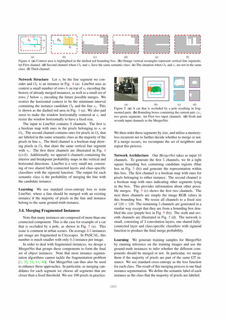
(a) (b) (c) (d) (e) (f)

Figure 4. (a) Context area is highlighted in the dashed red bounding box. (b) Orange vertical rectangles represent vertical line segments.

(c) First channel. (d) Second channel where Ok and si have the same semantic class. (e) The situation when Ok and si are not in the same

class. (f) Third channel.

Network Structure Let si be the line segment we con-

sider and Ok is an instance in Fig. 4 (a). LineNet uses as

context a small number of rows h on top of si encoding the

history of already merged instances, as well as a small set of

rows f below si encoding the future possible merges. We

restrict the horizontal context to be the minimum interval

containing the instance candidate Ok and the line si. This

is shown as the dashed red area in Fig. 4 (a). We also pad

zeros to make the window horizontally centered at si and

resize the window horizontally to have a fixed size.

The input to LineNet contains 9 channels. The first is

a boolean map with ones in the pixels belonging to si or

Ok. The second channel contains ones for pixels in Ok that

are labeled in the same semantic class as the majority of the

pixels in line si. The third channel is a boolean map show-

ing pixels in Ok that share the same vertical line segment

with si. The first three channels are illustrated in Fig. 4

(c)-(f). Additionally, we append 6 channels containing the

interior and breakpoint probability maps in the vertical and

horizontal directions. LineNet is a very small net, consist-

ing of two shared fully-connected layers and class-specific

classifiers with the sigmoid function. The output for each

semantic class is the probability of merging the line with

the candidate instance.

Learning We use standard cross-entropy loss to train

LineNet, where a line should be merged with an existing

instance if the majority of pixels in the line and instance

belong to the same ground-truth instance.

3.4. Merging Fragmented Instances

Note that many instances are composed of more than one

connected component. This is the case for example of a car

that is occluded by a pole, as shown in Fig. 5 (a). This

issue is common in urban scenes. On average 3.5 instances

per image are fragmented in Cityscapes. In PASCAL, this

number is much smaller with only 0.3 instance per image.

In order to deal with fragmented instances, we design a

MergerNet that groups these components to form the final

set of object instances. Note that most instance segmen-

tation algorithms cannot tackle the fragmentation problem

[3, 26, 18, 41, 40]. Our MergerNet can thus also be used

to enhance these approaches. In particular, as merging can-

didates for each segment we choose all segments that are

closer than a fixed threshold. We use 100 pixels in practice.

(a) (b) (c) (d)

Figure 5. (a) A car that is occluded by a pole resulting in frag-

mented parts. (b) Bounding boxes containing the current pair, i.e.,

two green segments. (c) First two input channels. (d) Sixth and

seventh input channels to the MergerNet.

We then order these segments by size, and utilize a memory-

less recurrent net to further decide whether to merge or not.

If a merge occurs, we recompute the set of neighbors and

repeat this process.

Network Architecture Our MergerNet takes as input 10

channels. To generate the first 5 channels, we fit a tight

square bounding box containing candidate regions (blue

box in Fig. 5 (b)) and generate the representation within

this box. The first channel is a boolean map with ones for

pixels belonging to either instance. The second channel is

a boolean map with ones indicating other segments lying

in the box. This provides information about other possi-

ble merges. Fig. 5 (c) shows the first two channels. The

next three channels are simply the image RGB values in

this bounding box. We resize all channels to a fixed size

of 128× 128. The remaining 5 channels are generated in a

similar way except that they are from a bounding box dou-

bled the size (purple box in Fig. 5 (b)). The sixth and sev-

enth channels are illustrated in Fig. 5 (d). The network is

small, consisting of 3 convolution layers, one shared fully-

connected layer and class-specific classifiers with sigmoid

function to produce the final merge probability.

Learning We generate training samples for MergerNet

by running inference on the training images and use the

ground-truth instances to infer whether the different com-

ponents should be merged or not. In particular, we merge

them if the majority of pixels are part of the same GT in-

stance. We use standard cross-entropy as the loss function

for each class. The result of this merging process is our final

instance segmentation. We define the semantic label of each

instance as the class that the majority of pixels are labeled.

3499

Method person rider car truck bus train mcycle bicycle

Uhrig et al. [36] 12.5 11.7 22.5 3.3 5.9 3.2 6.9 5.1

RecAttend [31] 9.2 3.1 27.5 8.0 12.1 7.9 4.8 3.3

Levinkov et al. [19] 6.5 9.3 23.0 6.7 10.9 10.3 6.8 4.6

InstanceCut [18] 10.0 8.0 23.7 14.0 19.5 15.2 9.3 4.7

SAIS [16] 14.6 12.9 35.7 16.0 23.2 19.0 10.3 7.8

DWT [3] 15.5 14.1 31.5 22.5 27.0 22.9 13.9 8.0

DIN [1] 16.5 16.7 25.7 20.6 30.0 23.4 17.1 10.1

Our SGN 21.8 20.1 39.4 24.8 33.2 30.8 17.7 12.4

Method AP AP 50% AP 100m AP 50m

Uhrig et al. [36] 8.9 21.1 15.3 16.7

RecAttend [31] 9.5 18.9 16.8 20.9

Levinkov et al. [19] 9.8 23.2 16.8 20.3

InstanceCut [18] 13.0 27.9 22.1 26.1

SAIS [16] 17.4 36.7 29.3 34.0

DWT [3] 19.4 35.3 31.4 36.8

DIN [1] 20.0 38.8 32.6 37.6

Our SGN 25.0 44.9 38.9 44.5

Table 1. AP results on Cityscapes test. The entries with the best performance are bold-faced.

Method person rider car truck bus train motorcycle bicycle AP AP 50%

DWT-non-ranking [3] 15.5 13.8 33.1 23.6 39.9 17.4 11.9 8.8 20.5 -

DWT-ranking [3] 15.5 13.8 33.1 27.1 45.2 14.5 11.9 8.8 21.2 -

SAIS [16] - - - - - - - - - 32.4

Our SGN 21.3 19.5 41.2 33.4 49.9 40.7 14.7 13.0 29.2 49.4

Table 2. AP results on Cityscapes val. The entries with the best performance are bold-faced.

4. Experimental Evaluation

We evaluate our method on the challenging dataset

Cityscapes [7] as well as PASCAL VOC 2012 [11]. We

focus our experiments on Cityscapes as it is much more

challenging. On average, it contains 17 object instances per

image vs 2.4 in PASCAL.

Dataset The Cityscapes dataset [7] contains imagery of

complex urban scenes with high pixel resolution of 1, 024×2, 048. There are 5, 000 images with high-quality anno-

tations that are split into subsets of 2, 975 train, 500 val

and 1, 525 test images, respectively. We use images in the

train subset with fine labels to train our networks. For the

instance segmentation task, there are 8 classes, including

different categories of people and vehicles. Motion blur,

occlusion, extreme scale variance and imbalanced class dis-

tribution make this dataset extremely challenging.

Metrics The metric used by Cityscapes is Average Preci-

sion (AP). It is computed at different thresholds from 0.5

to 0.95 with step-size of 0.05 followed by averaging. We

report AP at 0.5 IoU threshold and AP within a certain

distance. As pointed in [3, 1], AP favors detection-based

methods. Thus we also report the Mean Weighted Coverage

(MWCov) [31, 37], which is the average IoU of prediction

matched with ground-truth instances weighted by the size

of the ground-truth instances.

Implementation Details For our breakpoint predic-

tion network, we initialize conv1 to conv5 layers from

VGG16 [35] pre-trained on Imagenet [34]. We use random

initialization for other layers. The learning rates to train the

breakpoint prediction network, LineNet and the MergerNet

are set to 10−5, 10−2 and 10

−3, respectively. We use SGD

with momentum for training. Following the method of [5],

we use the “poly” policy to adjust the learning rate. We train

the breakpoint prediction network for 40k iterations, while

LineNet and MergerNet are trained using 20k iterations. To

alleviate the imbalance of class distribution for LineNet and

MergerNet, we sample training examples in mini-batches

by keeping equal numbers of positives and negatives. Fol-

lowing [3], we remove small instances and use semantic

scores from semantic segmentation to rank predictions for

{train, bus, car, truck}. For other classes, scores are set

to 1. By default, we use semantic segmentation prediction

from PSP [42] on Cityscapes and LRR [13] on PASCAL

VOC. We also conduct an ablation study of how the quality

of semantic segmentation influences our results.

Comparison to State-of-the-art As shown in Table 1,

our approach significantly outperforms other methods on all

classes. We achieve an improvement of 5% absolute and

25% in relative performance compared to state-of-the-art

reported on the Cityscapes website, captured at the moment

of our submission. We also report results on the validation

set in Table 2, where the improvement is even larger.

Influence of Semantic Segmentation We investigate the

influence of semantic segmentation in our instance predic-

tion approach. We compare the performance of our ap-

proach when using LRR [13], which is based on VGG-16,

with PSP [42], which is based on Resnet-101. As shown

in Table 3, we achieve reasonable results using LRR, how-

ever, much better results are obtained when exploiting PSP.

Results improve significantly in both cases when using the

MergerNet. Note that LineNet and MergerNet are not fine-

tuned for LRR prediction.

Influence of Size As shown in Fig. 7, as expected, small

instances are more difficult to detect than the larger ones.

Influence of LineNet Parameters The contextual infor-

mation passed to LineNet is controlled by the number of

history rows h, as well as the number of rows f encoding

the future information. As shown in Table 4, LineNet is not

3500

LRR [13] PSP [42] MergerNet AP AP 50% MWCov

X 20.0 37.8 64.3

X X 21.7 40.9 66.4

X 25.2 43.8 70.6

X X 29.2 49.4 74.1

Table 3. Cityscapes val with different semantic segm. methods.

Metric h1f1 h1f3 h1f5 h3f1 h3f3 h3f5 h5f1 h5f3 h5f5

AP 25.3 25.2 25.2 24.8 24.9 24.9 24.9 25.2 25.0

AP 50% 44.0 44.1 43.8 43.2 43.6 43.3 43.3 43.7 43.5

MWCov 71.4 71.3 71.6 70.9 71.5 71.3 71.1 71.6 71.4

Table 4. Cityscapes val results in terms of AP, AP 50%, MWCov.

sensitive to the context parameters while local information

is sufficient. In the following experiments, we select the

entry “h1f5” by considering both AP and MWCov.

Heuristic Methods vs LineNet We compare LineNet to

two heuristic baseline methods. The first takes the union

of vertical and horizontal breakpoints and class boundaries

from PSP. We thin them into one pixel width to get the in-

stance boundary map. In the foreground area defined via

the PSP semantic segmentation map, we set the instance

boundary as 0 and then take connected components as in-

ferred instances. Post-processing steps, such as removing

small objects and assigning scores, are exactly the same as

in our approach. We name this method “con-com”.

Our second baseline is called “heuristic”. Instead of us-

ing LineNet, we simply calculate a relationship between

two neighboring line segments (current line segment and

neighboring line segment in previous row) to make a deci-

sion. The value we compute includes the IoU value, ratio of

the overlaps with the other line segment and ratio of vertical

line segments connecting them in the overlapping area. If

each value and their summation are higher than the chosen

thresholds, we merge the two line segments. This strategy

simply makes decisions based on the current line segment

pair – no training is needed.

As shown in Table 6, on average, the heuristic strat-

egy outperforms the simple connected component method

in terms of all metrics. This clearly shows the benefit of

using line segments. LineNet outperforms both heuristic

methods, demonstrating the advantage of incorporating a

network to perform grouping. The connected component

method performs quite well on classes such as car and bus,

but performs worse on person and motorcycle. This sug-

gests that boundaries are more beneficial to instances with

compact shape than to those with complex silhouettes. Our

approach, however, works generally well on both, complex

and compact shapes, and further enables networks to correct

errors that exist in breakpoint maps.

Influence of MergerNet Parameters A parameter of the

MergerNet is the max distance between foreground regions

MethodAPr

APr

avg0.5 0.6 0.7 0.8 0.9

PFN [23] 58.7 51.3 42.5 31.2 15.7 39.9

Arnab et al. [2] 58.3 52.4 45.4 34.9 20.1 42.2

MPA 3-scale [26] 62.1 56.6 47.4 36.1 18.5 44.1

DIN [1] 61.7 55.5 48.6 39.5 25.1 46.1

Our SGN 61.4 55.9 49.9 42.1 26.9 47.2

Table 5. APr on PASCAL val.

in a candidate pair. To set the value, we first predict in-

stances with LineNet on the train subset and compute statis-

tics. We show recall of pairs that need to be merged vs

distance in Fig. 8(a) and the number of pairs with distance

smaller than a threshold vs distance in Fig. 8(b). We plot the

performance with respect to different maximum distances

used to merge in Fig. 8(c) and (d). Distance 0 means that

the MergerNet is not utilized. The MergerNet with different

parameters consistently improves performance. The results

show that the MergerNet with 150 pixels as the maximum

distance performs slightly worse than MergerNet with 50

and 100 pixels. We hypothesize that with larger distances,

more false positives confuse MergerNet during inference.

Visual Results We show qualitative results of all inter-

mediate steps in our approach on Cityscapes val in Fig. 6.

Our method produces high-quality breakpoints, instance in-

terior, line segments and final results, for objects of different

scales, classes and occlusion levels. The MergerNet works

quite well as shown in Fig. 6 as well as on the train object in

Fig. 9(b). Note that predictions with IoU higher than 0.5 are

assigned colors of their corresponding ground-truth labels.

Failure Modes Our method may fail if errors exist in the

semantic segmentation maps. As shown in Fig. 9(b), a small

part of the train is miss-classified by PSP. So the train is

broken into two parts. Our method may also miss extremely

small instances, such as some people in Fig. 9(e) and (f).

Further, when several complex instances are close to each

other, we may end up grouping them as shown in Fig. 9(g)

and (h). The MergerNet sometimes also aggregates differ-

ent instances such as the two light green cars in Fig. 9(a).

Results on PASCAL VOC We also conduct experiments

on PASCAL VOC 2012 [11], which contains 20 classes.

As is common practice, for training images, we addition-

ally use annotations from the SBD dataset [14], resulting in

10, 582 images with instance annotation. For the val subset,

we used 1, 449 images from VOC 2012 val set. There is no

overlap between training and validation images. Following

common practice, we compare with state-of-the-art on the

val subset since there is no held-out test set. Note that the

LRR model we use is pre-trained on MS COCO [25], which

is also used by DIN [1] for pre-training.

We use APr [15] as the evaluation metric, representing

the region AP at a specific IoU threshold. Following [25, 7],

3501

input image hori. breakpoint map vert. breakpoint map hori. line segments

vert. line segments our result without MergerNet our result with MergerNet ground-truth

input image hori. breakpoint map vert. breakpoint map hori. line segments

vert. line segments our result without MergerNet our result with MergerNet ground-truth

Figure 6. Qualitative results of all intermediate results and final prediction.

Method person rider car truck bus train motorcycle bicycle Average

con-com 16.6 / 70.8 9.1 / 57.2 40.0 / 89.6 29.8 / 84.5 46.6 / 88.8 21.1 / 68.5 7.4 / 48.9 6.1 / 49.1 22.1 / 69.7

heuristic 20.4 / 71.7 16.1 / 62.0 36.6 / 87.3 29.0 / 80.8 38.5 / 89.3 19.4 / 68.7 10.1 / 54.2 8.4 / 50.9 23.6 / 70.6

Linenet 20.2 / 71.7 17.8 / 62.9 38.5 / 88.2 32.0 / 83.9 46.4 / 88.6 23.3 / 69.5 14.1 / 59.4 9.4 / 48.4 25.2 / 71.6

Table 6. Results on Cityscapes val in terms of AP / MWCov.

0

0.2

0.4

0.6

0.8

1

1 100 10000 1000000

Figure 7. IoU as a function of ground-truth sizes.

we average APr at IoU threshold ranging from 0.5 to 0.9

with step-size 0.1 (instead of 0.1 to 0.9). We believe that

APr at higher IoU thresholds are more informative.

As shown in Table 5 our method outperforms DIN [1]

by 1.1 points in terms of APravg. We also achieve better

performance for IoU higher than 0.6. This result demon-

strates the quality of masks generated by our method. Our

method takes about 2.2s with LineNet “h1f5” and 1.6s with

LineNet “h1f1” per image using one Titan X graphics card

and an Intel Core i7 3.50GHZ CPU using a single thread on

PASCAL VOC. This includes the CPU time.

5. Conclusion

We proposed Sequential Grouping Networks (SGN) for

object instance segmentation. Our approach employs a

sequence of simple networks, each solving a more com-

plex grouping problem. Object breakpoints are composed

to create line segments, which are then grouped into con-

nected components. Finally, the connected components are

grouped into full objects. Our experiments showed that our

approach significantly outperforms existing approaches on

the challenging Cityscapes dataset and works well on PAS-

CAL VOC. In our future work, we plan to make our frame-

work end-to-end trainable.

6. Acknowledgments

This work is in part supported by NSERC, CFI, ORF, ERA,

CRC as well as Research Grants Council of the Hong Kong SAR

(project No. 413113). We also acknowledge GPU donations from

NVIDIA.

3502

0

0.2

0.4

0.6

0.8

1

0 50 100 150 200 250 300

Recall

Distance

Pair Recall versus Distance

0

20

40

60

80

100

120

0 50 100 150 200 250 300#P

air

per

Im

.

Distance

#Pair per Im. versus Distance

70

71

72

73

74

75

0 50 100 150

MW

Cov

Distance

MWCov versus Distance

(a) (b) (c) (d)

Figure 8. (a) Recall of merge pairs as a function of max distance. (b) Number of pairs with distance of foreground regions smaller than a

distance. (c) AP with respect to different maximum distances. (d) MWCov with respect to different maximum distances.

(a)

(b)

(c)

(d)

(e)

(f)

(g)

(h)

input image semantic segmentation [42] our results ground-truthFigure 9. Qualitative results of our method.

3503

References

[1] A. Arnab and P. H. Torr. Pixelwise instance segmentation

with a dynamically instantiated network. In CVPR, 2017. 1,

2, 5, 6, 7

[2] A. Arnab and P. H. S. Torr. Bottom-up instance segmentation

using deep higher-order crfs. CoRR, 2016. 2, 6

[3] M. Bai and R. Urtasun. Deep watershed transform for in-

stance segmentation. CoRR, 2016. 1, 2, 4, 5

[4] L. Castrejon, K. Kundu, R. Urtasun, and S. Fidler. Annotat-

ing object instances with a polygon-rnn. In CVPR, 2017. 1,

2

[5] L. Chen, G. Papandreou, I. Kokkinos, K. Murphy, and A. L.

Yuille. Deeplab: Semantic image segmentation with deep

convolutional nets, atrous convolution, and fully connected

crfs. CoRR, 2016. 3, 5

[6] L.-C. Chen, G. Papandreou, I. Kokkinos, K. Murphy, and

A. L. Yuille. Semantic image segmentation with deep con-

volutional nets and fully connected crfs. In ICLR, 2015. 1,

3

[7] M. Cordts, M. Omran, S. Ramos, T. Rehfeld, M. Enzweiler,

R. Benenson, U. Franke, S. Roth, and B. Schiele. The

cityscapes dataset for semantic urban scene understanding.

In CVPR, 2016. 1, 5, 6

[8] J. Dai, K. He, and J. Sun. Convolutional feature masking for

joint object and stuff segmentation. In CVPR, 2015. 1

[9] J. Dai, K. He, and J. Sun. Instance-aware semantic segmen-

tation via multi-task network cascades. CVPR, 2016. 1

[10] J. Dai, Y. Li, K. He, and J. Sun. R-FCN: object detection via

region-based fully convolutional networks. CoRR, 2016. 1

[11] M. Everingham, L. Van Gool, C. K. Williams, J. Winn, and

A. Zisserman. The pascal visual object classes (voc) chal-

lenge. IJCV, 2010. 5, 6

[12] C. Fu, W. Liu, A. Ranga, A. Tyagi, and A. C. Berg. DSSD :

Deconvolutional single shot detector. CoRR, 2017. 3

[13] G. Ghiasi and C. C. Fowlkes. Laplacian reconstruction and

refinement for semantic segmentation. CoRR, 2016. 5, 6

[14] B. Hariharan, P. Arbelaez, L. Bourdev, S. Maji, and J. Malik.

Semantic contours from inverse detectors. In ICCV, 2011. 6

[15] B. Hariharan, P. Arbelaez, R. Girshick, and J. Malik. Simul-

taneous detection and segmentation. In ECCV. 2014. 1, 6

[16] Z. Hayder, X. He, and M. Salzmann. Shape-aware instance

segmentation. CoRR, 2016. 1, 2, 5

[17] L. Jin, Z. Chen, and Z. Tu. Object detection free instance

segmentation with labeling transformations. CoRR, 2016. 2

[18] A. Kirillov, E. Levinkov, B. Andres, B. Savchynskyy, and

C. Rother. Instancecut: from edges to instances with multi-

cut. CoRR, 2016. 2, 4, 5

[19] E. Levinkov, S. Tang, E. Insafutdinov, and B. Andres. Joint

graph decomposition and node labeling by local search.

CoRR, 2016. 5

[20] K. Li, B. Hariharan, and J. Malik. Iterative instance segmen-

tation. CVPR, 2016. 2

[21] Y. Li, H. Qi, J. Dai, X. Ji, and Y. Wei. Fully convolutional

instance-aware semantic segmentation. CoRR, 2016. 2

[22] X. Liang, Y. Wei, X. Shen, Z. Jie, J. Feng, L. Lin, and

S. Yan. Reversible recursive instance-level object segmen-

tation. arXiv, 2015. 2

[23] X. Liang, Y. Wei, X. Shen, J. Yang, L. Lin, and S. Yan.

Proposal-free network for instance-level object segmenta-

tion. arXiv, 2015. 2, 6

[24] T. Lin, P. Dollar, R. B. Girshick, K. He, B. Hariharan, and

S. J. Belongie. Feature pyramid networks for object detec-

tion. CoRR, 2016. 3

[25] T.-Y. Lin, M. Maire, S. Belongie, J. Hays, P. Perona, D. Ra-

manan, P. Dollar, and C. L. Zitnick. Microsoft coco: Com-

mon objects in context. In ECCV. 2014. 6

[26] S. Liu, X. Qi, J. Shi, H. Zhang, and J. Jia. Multi-scale patch

aggregation (mpa) for simultaneous detection and segmenta-

tion. CVPR, 2016. 2, 4, 6

[27] J. Long, E. Shelhamer, and T. Darrell. Fully convolutional

networks for semantic segmentation. In CVPR, 2015. 1, 3

[28] A. Newell and J. Deng. Associative embedding: End-to-end

learning for joint detection and grouping. CoRR, 2016. 2

[29] P. H. O. Pinheiro, R. Collobert, and P. Dollar. Learning to

segment object candidates. In NIPS, 2015. 1

[30] P. H. O. Pinheiro, T. Lin, R. Collobert, and P. Dollar. Learn-

ing to refine object segments. In ECCV, 2016. 1, 3

[31] M. Ren and R. S. Zemel. End-to-end instance segmentation

and counting with recurrent attention. CoRR, 2016. 1, 2, 5

[32] S. Ren, K. He, R. Girshick, and J. Sun. Faster r-cnn: Towards

real-time object detection with region proposal networks. In

NIPS, 2015. 1

[33] B. Romera-Paredes and P. H. S. Torr. Recurrent instance

segmentation. CoRR, 2015. 1, 2

[34] O. Russakovsky, J. Deng, H. Su, J. Krause, S. Satheesh,

S. Ma, Z. Huang, A. Karpathy, A. Khosla, M. S. Bernstein,

A. C. Berg, and F. Li. Imagenet large scale visual recognition

challenge. International Journal of Computer Vision, 2015.

5

[35] K. Simonyan and A. Zisserman. Very deep convolutional

networks for large-scale image recognition. ICLR, 2014. 3,

5

[36] J. Uhrig, M. Cordts, U. Franke, and T. Brox. Pixel-level

encoding and depth layering for instance-level semantic la-

beling. CoRR, 2016. 2, 5

[37] S. Wang, M. Bai, G. Mattyus, H. Chu, W. Luo, B. Yang,

J. Liang, J. Cheverie, S. Fidler, and R. Urtasun. Torontocity:

Seeing the world with a million eyes. CoRR, 2016. 5

[38] S. Xie and Z. Tu. Holistically-nested edge detection. In

ICCV, 2015. 3

[39] F. Yu and V. Koltun. Multi-scale context aggregation by di-

lated convolutions. CoRR, 2015. 3

[40] Z. Zhang, S. Fidler, and R. Urtasun. Instance-level segmen-

tation for autonomous driving with deep densely connected

mrfs. In CVPR, 2016. 1, 2, 4

[41] Z. Zhang, A. G. Schwing, S. Fidler, and R. Urtasun. Monoc-

ular object instance segmentation and depth ordering with

cnns. CoRR, 2015. 1, 2, 4

[42] H. Zhao, J. Shi, X. Qi, X. Wang, and J. Jia. Pyramid scene

parsing network. CoRR, 2016. 5, 6, 8

3504