NBER WORKING PAPER SERIES

SEX RATIOS, ENTREPRENEURSHIP, AND ECONOMIC GROWTH IN THE PEOPLE’SREPUBLIC OF CHINA

Shang-Jin WeiXiaobo Zhang

Working Paper 16800http://www.nber.org/papers/w16800

NATIONAL BUREAU OF ECONOMIC RESEARCH1050 Massachusetts Avenue

Cambridge, MA 02138February 2011

This research is supported by U.S. National Science Foundation grant SES-1024574, which we gratefullyacknowledge. The authors would like to thank Patrick Bolton, Qingyuan Du, Lena Edlund, Amit Khandelwal,Hongbin Li, Rick Mishkin, Meng Xin, Nancy Qian and seminar/conference participants at the NBERconferences in Cambridge and Beijing, annual Chinese Economists Society meetings in Xiamen, ColumbiaUniversity, Cornell University, National University of Singapore, and Carleton University for helpfuldiscussions, and Kyle Gerry, Joy Glazener, and Jin Yang for assistance. All errors are the authors’responsibilities. The views expressed herein are those of the authors and do not necessarily reflectthe views of the National Bureau of Economic Research.

NBER working papers are circulated for discussion and comment purposes. They have not been peer-reviewed or been subject to the review by the NBER Board of Directors that accompanies officialNBER publications.

© 2011 by Shang-Jin Wei and Xiaobo Zhang. All rights reserved. Short sections of text, not to exceedtwo paragraphs, may be quoted without explicit permission provided that full credit, including © notice,is given to the source.

Sex Ratios, Entrepreneurship, and Economic Growth in the People’s Republic of ChinaShang-Jin Wei and Xiaobo ZhangNBER Working Paper No. 16800February 2011JEL No. E2,F3,F43,J1,J2,O1,O4

ABSTRACT

China experiences an increasingly severe relative surplus of men in the pre-marital age cohort. Theexisting literature on its consequences focuses mostly on negative aspects such as crime. In this paper,we provide evidence that the imbalance may also stimulate economic growth by inducing moreentrepreneurship and hard work. First, new domestic private firms – an important engine of growth– are more likely to emerge from regions with a higher sex ratio imbalance. Second, the likelihoodfor parents with a son to be entrepreneurs rises with the local sex ratio. Third, households with a sonin regions with a more skewed sex ratio demonstrate a greater willingness to accept relatively dangerousor unpleasant jobs and supply more work days. In contrast, the labor supply pattern by householdswith a daughter is unrelated to the sex ratio. Finally, regional GDP tends to grow faster in provinceswith a higher sex ratio. Since the sex ratio imbalance will become worse in the near future, this growtheffect is likely to persist.

Shang-Jin WeiGraduate School of BusinessColumbia UniversityUris Hall 6193022 BroadwayNew York, NY 10027-6902and NBERshangjin.wei@columbia.edu

Xiaobo ZhangInternational Food Policy Research Institute2033 K Street, NWWashington, DC 20006x.zhang@cgiar.org

1

1. Introduction

This paper explores the implications of sex ratio imbalance for entrepreneurial activities

and economic growth in China.

A sex ratio imbalance in the marriage age cohort – too many men relative to women – is

a common demographic feature in many Asian economies, including Korea, India, Vietnam,

Singapore, Taiwan, and Hong Kong. In many such economies, parents voluntarily limit the

number of children they wish to have. This, together with a strong preference for sons, and the

availability of inexpensive technology to screen the gender of a fetus (most commonly by

Ultrasound B) to abort the unwanted pregnancy, leads parents to engage in sex selective

abortions in favor of sons. But nowhere else has a more skewed sex ratio than China today,

where a strict family planning policy has restricted the number of children most families can

have to one or two and has greatly reinforced the incentive for sex selective abortions. In 1980,

when the strict family planning policy was first introduced in China, its sex ratio at birth was

1.07 boys per girl, which was basically in line with the natural rate observed in most countries.

The Chinese sex ratio deteriorated steadily to 1.12 boys per girl in 1990, 1.18 in 2000, and 1.22

in 2007 (Li, 2007; Zhu, Lu, and Hesketh, 2009). As a result, roughly one out of every nine young

men today has no realistic hope to get married, mathematically speaking. In some provinces, one

out of every six men cannot get married. This situation is projected to deteriorate in the next ten

years based on the population census data.

The existing literature has identified several negative consequences of a serious sex ratio

imbalance. First, the scale of involuntarily single men is frightening. For example, the number of

excess Chinese men under age 20 exceeded 32 million in 2005 (Zhu, Lu, and Hesketh, 2009).

This number is greater than the entire male population of Italy or Canada. Second, the imbalance

may cause crimes. Using data across Chinese provinces, Edlund, Li, Yi, and Zhang (2007)

estimate that every one basis point increase in the sex ratio (e.g., from 1.10 to 1.11 boys per girl)

raises violent and property crime rates by 3%, and the rise in the sex ratio imbalance may

account for up to one-seventh of the overall rise in crime in China. Den Boer and Hudson (2004)

boldly hypothesize that the sex ratio imbalance should generate security concerns for other

countries since the one with a high sex ratio “might actively desire to send its surplus young

males to give their lives in a national cause,” although they provide no rigorous data analysis to

back up their theory. Third, the imbalance may also trigger competitive savings among

2

households – men and households with sons forego current consumption to accumulate wealth in

order to improve a young man’s standing in the marriage market relative to other men. This

increase in the savings rate is inefficient since it does not alter the number of unmarried men in

the aggregate. Wei and Zhang (2009) estimate that about half the increase in the household

savings rate in China during 1990-2005 can be attributed to the rise in the sex ratio. By raising

the aggregate savings, the sex ratio imbalance contributes to China’s current account surplus,

which is a source of international frictions. Since some believe that China’s current account

surplus was a significant factor in the asset price bubbles during 2002-2007 (according to

Greenspan, 2009, and Rajan, 2010, among others), the sex ratio imbalance, by an extension of

that logic, is a contributing factor to the onset of the 2007-2009 global financial crisis.

In this paper, we study a possibly positive effect of the sex ratio imbalance on economic

growth. If the family wealth of a man relative to those of other men is a sorting variable for a

man’s relative standing in the marriage market, then a rise in the sex ratio can inspire men and

parents with a son to find ways to accumulate more wealth. Working harder or longer, and

becoming more entrepreneurial are ways to achieve this objective. As a result, the economy may

grow faster than it would have otherwise. As far as we know, this effect has never been

investigated before.

We conduct the empirical analysis using data from censuses of firms, censuses and

surveys of population, and household surveys. Several reasons make China a particularly good

candidate for this research topic. First, China presents one of the fastest increases in the sex ratio

in the world due to its draconian family planning policy. As a result, there is a better chance to

detect this growth effect if one exists. Second, a within-country study has advantages over cross-

country studies as the legal system and other institutions can be more plausibly held constant

across regions within a country than across countries. As a very large country, there are many

sub-national geographic units in China that allow us to have sufficient statistical power when

exploring regional variations. Moreover, due to government restrictions on household

registrations, internal mobility for marriage purpose is low (nearly 90% of marriages take place

between men and women from the same county; see Wei and Zhang, 2009). This makes each

marriage market highly localized. Third, while the Chinese economy is about half the size of the

United States on a PPP-adjusted basis, the contribution of Chinese growth to the incremental

world GDP has been the largest in the world since 2002 (IMF 2009). Therefore, understanding

3

the determinants of Chinese growth has intrinsic value for international macroeconomics due to

its direct global implications.

The empirical results not only support the hypothesis qualitatively, but also are

significant quantitatively. Based on the two most recent censuses of firms, we estimate that an

increase in the sex ratio by one standard deviation can account for about half of the extensive

margin of the private sector growth (i.e., the birth of new private firms) across regions.

To address concerns about possible biases due to measurement errors, endogeneity, and

missing regressors, we employ four different approaches that complement each other. Both an

instrumental variable approach and a placebo test suggest that there is a causal effect from a

higher sex ratio to more entrepreneurship. Two different household-level data provide additional

information. For example, from a random sample of a national population survey in 2005, we

document that parents with a son are more likely to be entrepreneurs in regions with a higher sex

ratio. In comparison, the likelihood for parents with a daughter to be entrepreneurs is

uncorrelated with the local sex ratio. From a separate survey of rural households in 2002, we

estimate that households with a son respond to a rise in the sex ratio by a combination of

working more days off farms (including as migrant workers) and becoming more willing to

accept unpleasant or relatively dangerous jobs. In contrast (but consistent with our hypothesis),

the labor supply pattern of daughter-households is not linked to the local sex ratio.

Finally, to capture the general equilibrium effect, we also directly check whether the

growth of per capita GDP across regions is linked to the local sex ratio imbalance and find that

the answer is affirmative. We estimate that about 20% of the growth rate of GDP per capita in

recent years can be attributed to a rise in the sex ratio. Since the sex ratio imbalance is projected

to become worse in the next decade, this effect may become relatively more important over time.

The rest of the paper is organized in the following way. In Section 2, we develop the

argument more fully and connect to related literatures. In Section 3, we provide statistical

evidence. Finally, in Section 4, we conclude and discuss possible future research.

2. The connection between the hypothesis and the existing literature

The hypothesis that a higher sex ratio can be an important driver for entrepreneurial

activities in China is related to four sets of literature: (a) status goods, (b) economics of family,

4

(c) entrepreneurship, and (d) causes and consequences of sex ratio imbalance. Each of them is

too vast to be referenced comprehensively here. Instead, we selectively discuss some of them,

with a view to highlight some insight most relevant for our empirical investigation.

Several theoretical papers have pointed out a connection between concerns for status

(one’s relative position in a society), the savings rate, and the economic growth rate (Cole,

Mailath and Postlewaite, 1992; Cornero and Jeanne, 1999; and Hopkins and Kornienko, 2009).

When wealth defines one’s status in the marriage market, a greater concern for status may lead to

an increase in the growth rate. In principle, concerns for status could also produce the opposite

effect on savings and growth. In particular, if status is enhanced by conspicuous consumption,

then a greater concern for status can translate into a reduction in savings (Frank, 1985 and 2005).

It is interesting to note that, while many papers on the topic of status use competition in the

marriage market to illustrate the idea, the sex ratio is always assumed to be balanced. In other

words, no explicit comparative statistics are derived in terms of a rise in sex ratio imbalance.1

Du and Wei (2011b) develop a model that explores the effect of a higher sex ratio on

entrepreneurial activities. As it is the only model that explicitly studies such a topic, we review it

with some details. The model features overlapping generations with two genders and a desire to

marry. Everyone lives for two periods, and can marry with a member of the opposite sex at the

beginning of the second period. There are two benefits associated with marriage. First, a husband

and a wife can pool their income and enjoy a partial public good feature of their joint

consumption. That is, the sum of their consumptions can be more than the sum of their incomes.

Second, a married person derives additional emotional utility (or “love”) from his/her spouse.

The amount of emotional utility that a person can bring to her/his future spouse is a random

variable in the first period, but its value is revealed and becomes public knowledge when she/he

enters the marriage market. Men and women are identical in their utility function and the form of

the budget constraint, except that by assumption only men can be entrepreneurs (a simplification

that is relaxed in an extension).

At the beginning of the second period, men and women voluntarily participate in the

marriage market. The matching between men and women is assumed to follow the Gale-

Shapely algorithm, which produces positive assortative matching in equilibrium. More precisely,

the best woman (defined by a combination of her wealth and the amount of emotional utility she

1 Edlund (1996) showed that a higher sex ratio imbalance may have a nonlinear impact on women’s status and dowry price.

5

can bring to her spouse) and the best man (also defined by a combination of wealth and

emotional utility) are matched; the second best woman and the second best man are matched;

and so on. If there are more men than women, the least attractive men are not married. By Gale

and Shapely (1962) and Roth and Sotomayer (1990), this equilibrium is both unique and stable.

In the first period, both men and women solve an optimization problem that takes into

account the effect of their choices on the outcome in the marriage market. A representative man

makes a sequential choice, first deciding whether to be an entrepreneur and then deciding on a

savings rate. Deciding to be an entrepreneur means to pay a fixed fee in order to get a random

draw on his productivity, which follows a binominal distribution. If his productivity is high, he

becomes a monopolistically competitive producer. If it is low, he becomes a worker. A

representative woman simply decides on a savings rate (as she is always a worker by a

simplifying assumption). Even with a balanced sex ratio, the Nash equilibrium would feature a

fraction of men becoming entrepreneurs. This is because entrepreneurship is a higher risk and a

higher return activity (relative to being a worker). Similar to a portfolio choice problem, there is

generally an interior solution in which a certain fraction of men choose the riskier activity.

Du and Wei (2011b) derive the following key proposition: As the sex ratio rises, as long

as it is beyond a (low) threshold, more men choose to become entrepreneurs. Here is the intuition.

By the structure of the model, successful entrepreneurs can always succeed in getting married,

but failed entrepreneurs do not. When the sex ratio exceeds a threshold, an increase in the sex

ratio raises the probability that a male worker will not get married, while it does not alter the

expected utility of being an entrepreneur (to a first-order approximation). If the utility from a

marriage is sufficiently large, more men would respond to a higher sex ratio by becoming

entrepreneurs.

The entrepreneurship model in Du and Wei (2011b) builds on the previous models in Du

and Wei (2010 and 2011a). While the effect of a higher sex ratio on the aggregate savings rate

and current account is the topic of Du and Wei (2010), one result from that model may be

relevant here. If resource allocation within a marriage depends on the husband and the wife’s

bargaining power, which in turn depends on the relative level of wealth that the two bring into

the marriage, then a representative woman could in principle raise her savings rate in response to

a higher sex ratio. This incentive faced by the representative woman – to protect the bargaining

power within a marriage – can offset an opposite incentive – to free ride on the higher expected

6

wealth from her future husband, and render the net effect of a higher sex ratio on a woman’s

savings rate ambiguous in general. We conjecture that a similar result could hold for

entrepreneurship: If women can also choose to be entrepreneurs, the net effect of a higher sex

ratio on the likelihood of women choosing to be entrepreneurs is ambiguous.

In a setup that features nontradable goods, Du and Wei (2011a) study channels through

which a higher sex ratio could reduce the value of the real exchange rate. One of the channels is

change in effective labor supply. In particular, as the sex ratio rises, under some conditions, men

choose to cut down leisure and supply more labor, with an aim to raise his wealth level and

improve his chance of success in the marriage market.

In terms of the empirical literature, Angrist (2002) examined variations in the sex ratio

across immigrant groups in the United States. He documented that a higher male/female sex ratio

has a large positive effect on the female marriage rate, and a large negative effect on female

labor market participation. Interestingly, he found that “higher sex ratios also appear to have

raised male earnings and the incomes of parents with young children.” These results are

consistent with what we report in this paper. It is important to note that Angrist (2002) did not

directly study the effects of sex ratio imbalance on entrepreneurial activities and economic

growth, which are the central focus of this paper.

There is an extensive literature in demography that documents the phenomenon of

unbalanced sex ratios in Asia (for example, Gu and Roy, 1995; Guilmoto, 2007; and Li, 2007).

Several papers have examined the determinants of sex ratio imbalance (including Das Gupta,

2005; Ebenstein, 2009; Edlund, 2009; Li and Zheng, 2009; and Bulte, Heerink and Zhang, 2011).

In an influential paper, Oster (2005) proposes that the prevalence of Hepatitis B is a significant

cause of the sex ratio imbalance in Asia. But this conclusion is later shown to be incorrect,

including by Lin and Luoh (2008) and Oster, Chen, Yu and Lin (2008). In a paper with a clever

instrumental variable approach, Qian (2008) shows that an improvement in the economic status

of women tends to reduce the sex ratio imbalance. Her instrument for the economic status of

women is the world price of tea, whose production is apparently particularly suitable for women

laborers. Wei and Zhang (2009) document that a higher sex ratio induces more savings. However,

the paper does not examine how labor supply and entrepreneurship respond to a change in the

sex ratio, which is the central focus of the current paper.

7

This discussion has clear implications for the empirical work in this paper. First, it is

interesting to find out if entrepreneurial activities are indeed linked to local sex ratios. Second,

given the hypothesized mechanisms, it is informative to check whether and how households with

a son and those with a daughter respond differently to a rise in the sex ratio. Third, given the

possibility that a higher sex ratio could also raise crime rates and have other consequences that

are potentially negative for economic growth, it is important to check the general equilibrium

effect – whether the economy-wide entrepreneurial activities and work effort increase on net, as

reflected in a higher overall growth rate, in response to a rise in the sex ratio.

Because Wei and Zhang (2009) have provided extensive evidence on the effects of a

higher sex ratio on savings behavior, we will not look at savings in this paper, and concentrate

instead on evidence related to entrepreneurship, work effort, and economic growth. In our view,

pursuing entrepreneurial activity (for higher income) and raising savings rate (out of a given

level of income) are two alternative ways to improve a household’s future wealth.

3. Statistical Evidence

We start by providing some basic facts about Chinese growth, which are summarized by

two 70% rules. We then use data from the two most recent censuses of manufacturing firms (in

1995 and 2004) to investigate whether local sex ratio imbalance is a predictor of the extent of

local entrepreneurial activities. To zoom in on possibly distinct responses by families with a son

versus those with a daughter, we turn to household-level evidence. Finally, to capture the general

equilibrium effect of a rise in the sex ratio, we conduct a panel growth regressions across

Chinese provinces over 1980-2005.

Background information: the two 70% rules about the Chinese growth

Since our first piece of evidence has to do with regional variations in entrepreneurial

activity, we work with the two most recent censuses of firms in 1995 and 2004, respectively, so

we can compute the growth in the number of firms by region. During this period, the country’s

industrial value added (at the current price) grew by 266%.

The growth of the private sector is a major part of the overall growth story. The private

sector is not just restricted to firms that were legally registered private firms. In fact, very few

8

firms were registered as private firms in the 1980s and 1990s. According to Huang (2009), many

private entrepreneurs at that time found it necessary to set up firms as nominally owned by local

governments (in the form of “township-and-village enterprises,” or “collectively owned firms”).

The goal was presumably to buy “protection” from the local government and to minimize the

risk of state expropriation. Such a practice was widespread and was called “private entrepreneurs

wearing a red hat.” Most entrepreneurs later engineered or attempted to engineer a change in the

firm ownership through which they would become a majority shareholder without injecting

much additional personal capital. Wu (2007) provides fascinating accounts of many

entrepreneurs both when they first “wore a red hat,” setting up a nominally collectively owned

firm, and when they tried to take off the hat, with uneven success rates. Because of the

recognition that most newly established “collectively owned firms” were private firms in

disguise, we adopt a broad definition of domestic private firms to include all such firms.

In Table 2, we report a simple exercise that decomposes the contributions to the growth

by firm ownership type (domestic private firms, majority state-owned firms, and foreign-

invested firms). Let X(total, t) be the industrial value added for the country as a whole in year t.

Define X(private, t), X(FDI, t), and X(SOE, t) to be the industrial value added in year t by the

domestic private sector, foreign invested firms, and state-owned firms, respectively. X(total, 04)

= X(private, 04) + X(FDI, 04) + X(SOE, 04). Let s(private, 95), s(FDI, 95), and s(SOE, 95) be

the share of the domestic private sector, foreign firms, and state-owned firms, respectively, in the

natural industrial output in 1995. We can decompose the overall growth rate into a weighted

average of the growth rates from the three types of firms:

(1) G(total) = X(total, 04)/X(total, 95) – 1

= g(private)*s(private, 95) + g(FDI) s(FDI, 95) + g(SOE) s(SOE, 95)

From this equation, we can compute the contribution of the domestic private sector to the

overall growth as: Private sector’s share of the contribution = g(private)s(private,95)/g(total) =

6.22*30.7%/2.66 = 71.9%. Similarly, foreign invested firms account for 30.8% of the overall

growth. The state sector accounts for -2.7% as many state-owned firms were either closed or

taken over by private firms. (Note that the decomposition of the real or nominal growth rates

gives the same result.)

9

We next decompose the private sector growth into the extensive margin (the growth in

the number of firms) and the intensive margin (the growth of average output per firm):

(2) Ln[X(private, 04)/X(private, 95)] = Ln[N(private, 04)/N(private, 95)] +

Ln{[X(private,04)/N(private, 04)]/ [X(private, 95)/N(private, 95)]}

The first term on the right hand side denotes the extensive margin, while the second term denotes

the intensive margin growth. In Table 3, we report the result of the decomposition. The

contribution of the extensive margin = the first term on RHS/LHS = 0.499/0.728 =68.5%.

To summarize, a little over 70% of the Chinese growth is attributable to the rise of the

private sector. In addition, almost 70% of the private sector growth is attributable to the birth and

the growth of new private firms2. Therefore, the birth and the growth of new private firms are a

significant part of the Chinese growth story.

Where are domestic private firms most likely to emerge?

We now examine whether there is any connection between the sex ratio and the extensive

margin of private sector growth. To reduce noise, we sort all counties into bins based on their sex

ratios for the age cohort of 5-19 in 1995. All counties in a bin have an identical sex ratio. In

Figure 1, we plot the average growth rate in the number of private firms across all counties in a

bin against the initial sex ratio imbalance for that bin. There is a strong positive relationship

between the growth of the count of private firms and the sex ratio. That is, regions with a more

skewed sex ratio are also places where new private firms are more likely to emerge.

Many factors could affect the birth and growth of new firms. The age structure of the

local population, the growth rate of the population, local income and education levels, local

industrial structure, and initial scale of the private sector could all matter. We are interested in

investigating whether the local sex ratio also plays a role. We do so by looking at variations in

the growth rate of the count of private firms and local sex ratios across 1790 counties,

conditional on other factors. The specification is as follows:

(3) Growth_in_firm-countk, 95-04, = β Sex_ratiok, 95, +Xk Γ +e k

2 Using a provincial level panel data, Li et. al. (2009) show entrepreneurship is a key engine of Chinese economic growth.

10

The result is reported in Column 1 of Table 4. The coefficient on initial sex ratio for the

age cohort 5-19 is 0.017 and statistically significant. To see if the effect of the local sex ratio

comes entirely from the local savings rate, we add log local bank savings balance per capita in

1995 as an additional control. The new regressor is not statistically significant. In any case, the

coefficient on the sex ratio is virtually unaffected. To see which sex ratio imbalance in terms of

age cohort matters the most, in Columns 3-5, we restrict the sex ratio to the age cohorts 5-9, 10-

14, and 15-19, respectively. All three seem to matter, but the cohort 10-14 seems to matter the

most. (While the coefficient on the sex ratio for the cohort 15-19 is not statistically significant, it

is mostly due to a greater standard error. The point estimate on the sex ratio in Columns 3 and 5

are virtually the same.) Interestingly, the coefficient on the sex ratio for each age cohort is

smaller than the one for the combined age cohort 5-19. Because most Chinese families have one

or two children, most families with children in the three age brackets do not overlap. As a result,

the effect of the sex ratio for the combined age cohort of 5-19 on the growth of private firms is

approximately the sum of the effects of the sex ratio for the three age cohorts.

As an alternative measure of the sex ratio, we use the average of the sex ratio for the age

cohort 5-19 in 1995 and the sex ratio for the age cohort of 4-18 in 2004 (inferred from the 1990

and the 2000 censuses, respectively). Due to the way that the sex ratios are reported in the two

censuses (at five-year intervals), we are not able to make an exact match in age cohort. In any

case, the regression results are reported in the last five columns of Table 4. In all regressions, the

coefficients on the sex ratio are positive and statistically significant. In other words, more

domestic private firms were established in regions with a higher sex ratio.

Possible problems with the OLS estimation and solutions

The OLS estimation may produce biased estimates. First, there could be errors in

measuring the sex ratio for the pre-marital age cohort. For example, with migration in and out of

a county (in spite of the policy restrictions), the sex ratio recorded in the population census may

not exactly correspond to the sex ratio in the local marriage market. The measurement errors tend

to produce a downward bias. Second, the sex ratio might be endogenous. In particular, the

positive association between the local sex ratio and the rate of growth of private firms may

reflect a reverse causality. For example, if private entrepreneurs have a stronger urge to have a

male heir to take over their business when they retire, then regions that happen to see a lot of

11

private firms may also exhibit a strong son preference and a high sex ratio imbalance. Third, the

sex ratio may be endogenous if it is correlated with some missing regressors. For example, in

spite of our best effort to control for determinants of the growth of private firms, there may be

other variables that are good predictors of future profitability in a region that are not captured by

our list of control variables. If these variables happen to be correlated with the local sex ratio, we

may find a positive association between the local sex ratio and the growth of local private firms

even when there is no direct economic association between the two.

To address these problems, we adopt four approaches that we hope would complement

and reinforce each other. First, we implement a two-stage least squared (2SLS) procedure in

which the local sex ratio is instrumented by variables that affect regional variations in the sex

ratio but are otherwise unlikely to affect directly the growth of local private firms. Second, we

use data from a population survey and check if the likelihood for parents with a son to become

entrepreneurs differs from parents with a daughter when the sex ratio rises. Third, we adopt a

placebo test on the growth of other profit-seeking firms. If the local sex ratio is simply a proxy

for missing regressors that help to forecast local growth potential, then the sex ratio should also

forecast the extensive margin growth of foreign-invested firms. Finally, we go to household-level

data where we can check possible interactions between local sex ratios and son-families in ways

that will also help us to rule out the endogeneity story. In particular, our theory suggests that son

families and daughter families may alter their work effort in different ways in response to a

common rise in the local sex ratio. We will discuss these approaches in turn.

Approach 1: Instrumental variable approach

A strategy to address both the measurement error problem and the endogeneity problem

is to employ an instrumental variable approach. A key determinant of the sex ratio imbalance is a

strict family planning policy introduced at the beginning of the 1980s3. We explore three

determinants of local sex ratios that are unlikely to be affected by the growth of local private

firms, and for which we can get data. First, while the goals of family planning are national, the

enforcement is local. Ebenstein (2009) proposes to use regional variations in the monetary

3 China’s family planning policy, commonly known as the “one-child policy,” has many nuances. Since 1979, the central government has stipulated that Han families in urban areas should normally have only child (with some exceptions). Ethnic Han families in rural areas can have a second child if the first one is a daughter (this is referred to as the “1.5 children policy” by Ebenstein, 2008). Ethnic minority (i.e., non-Han) groups are generally exempted from birth quotas. Non-Han groups account for a relatively significant share of local populations in Xinjiang, Yunnan, Ganshu, Guizhou, Inner Mongolia, and Tibet.

12

penalties for violating the birth quotas, originally collected by Scharping (2003), as instruments

for the local sex ratio. The idea is that, in regions with stiff penalties, parents may engage in

more sex-selective abortions, rather than paying a penalty and having more children. The

monetary penalty is often on the order of between one to five times the local average annual

household income. In addition, Ebenstein (2008) coded a dummy for the existence of extra fines

for violations at higher-order births. For example, an additional penalty may kick in on a family

for having the 3rd or 4th child in a one-child zone, or the 4th or 5th child in a two-child zone. Such

a non-linear financial penalty scheme was introduced by different local governments in different

years (if at all), generating variations across regions and over time. These two monetary penalty

variables constitute the first two candidates for our instrumental variables.4

The third instrumental variable explores the legal exemptions in the family planning

policy. While the policy imposes a strict birth quota on the Han ethnic group (the main ethnic

group in the country), the rest of the population (i.e., some 50 ethnic minority groups) do not

face or face much less stringent quotas. (The government allowed the exemption, possibly to

avoid criticism for using the family planning policy to marginalize the minority groups.) As a

result, the share of non-Han Chinese in the total population has risen from 6.7% in 1982 to 8.5%

in 2000 (Bulte, Heerink, and Zhang, 2011). Non-Han Chinese are not uniformly distributed

across space. In regions with relatively more ethnic minorities, marriages between Han and non-

Han peoples are not uncommon, reducing the competitive pressure for men in the marriage

market (Wei and Zhang, 2009). Therefore, the share of non-Han Chinese in the local population

offers another possible instrument.5

The first stage regressions are reported in Table 5. The dependent variable in the first

three regressions is the initial sex ratio for the age cohort 5-19, whereas that for the last three

regressions is the average sex ratio of the same age cohort over 1995 and 2004. The coefficients

on the share of the local population not subject to birth quotas are negative and statistically

significant in four regressions. This is consistent with the notion that sex selective abortions are

less prevalent when birth quotas apply to less people.

4 Edlund et al (2007) conduct some diagnostic checks and conclude that the level of financial penalties is uncorrelated with a region’s current economic status. We will perform and report a formal test on whether the proposed instruments and the error term in the second stage regressions are correlated. 5 In principle, variations in the cost of sex screening technology especially the use of an Ultrasound B machine (as documented by Li and Zheng, 2009), and the economic status of women (such as that documented in Qian 2008) could also be candidates for instrumental variables. Unfortunately, we do not have the relevant data. Note, however, for the validity of the instrumental variable regressions, we do not need a complete list of the determinants of the local sex ratio in the first stage.

13

The financial penalties for violating birth quotas generate a positive coefficient in all six

regressions (and significant in four of them). The dummy for the existence of extra penalties for

violations at higher-order births also produces a positive coefficient in all six regressions. These

results imply that a more severe penalty for violating legal birth quotas tends to induce parents to

more aggressively abort girls, resulting in a higher sex ratio imbalance. In other words, when the

penalties are light, many couples with daughters may opt to keep the daughter, pay the penalties,

and have another child, rather than abort the female fetus.

The adjusted R2’s are in the range between 0.09-0.21. The F statistics (for the null that all

slope parameters are jointly zeros) ranges from 22.8 to 37.5. The Kleibergen-Paap statistics (for

weak instruments) for five out of six regressions are greater than the Stock-Yogo 10% critical

value of 19.9. The Kleibergen-Paap statistic for the second regression is 18.1, which is greater

than the Stock-Yogo 15% critical value of 11.6.

The second stage regressions are reported in Table 6. The Durbin-Wu-Hausman test

easily rejects the null that the 2SLS and OLS estimates are the same in all six regressions,

implying that the sex ratio variable is likely to be either measured with errors or endogenous.

The Hansen’s J statistics do not reject the null that the instruments and the error term are

uncorrelated.6 The point estimates in Table 6 are generally much larger than their OLS

counterparts in Table 4. This suggests that the downward bias in Table 4 generated either by

missing regressors or by measurement errors is substantial.

We can compute the economic significance of the estimates. Using the most conservative

estimate in Column 6 of Table 6, an increase in the sex ratio by 3 basis points (e.g., from 1.08 to

1.11), which is equal to the increase in the average sex ratio from 1995 to 2004 (see Table 1),

generates an increase in the natural log number of private firms by 0.39 (=13x0.03). Since the

actual increase in log number of firms in this period is log 0.83 (see Row 3 of Table 1A), the rise

in the sex ratio can potentially explain 47% (=0.39/0.83) of the actual increase in the number of

private firms in China during this period. In other words, the economic impact of the rise in sex

ratio in promoting entrepreneurial activities in rural China is potentially very big.

6 In household-level regressions to be reported in Tables 11 and 12, we check if the ethnic minorities have a different labor supply pattern from Han Chinese, holding constant local sex ratio imbalance and other determinants of labor supply, and cannot reject the null that there is no difference.

14

We now perform similar regressions for the urban sample, and report the results in Table

7. The first two columns report OLS results, where the local sex ratio either at the beginning of

the period (1995) or averaged over 1995 and 2004 is positive and statistically significant.

In columns 3 and 4 of Table 7, we conduct 2SLS estimation. Again, the coefficient on the

sex ratio is positive and statistically significant in both cases. This is consistent with the notion

that a higher sex ratio imbalance has induced more people to engage in entrepreneurial activities.

It is noteworthy that the IV coefficients on the sex ratio variable for the urban sample in

Table 7 (0.08 and 0.06) are smaller than the corresponding coefficients for the rural sample in

Table 6 (between 0.13 and 0.20). Using the point estimate in the last column of Table 7 (0.06),

an increase in the sex ratio in the urban area by 3 basis points (e.g., from 1.08 to 1.11) would

generate an increase in the natural log number of private firms by 0.18 (=6*0.03), which is about

20% of the actual increase in the number of private firms during this period. While this number

is smaller than for the rural sample, it is still economically significant.

Approach 2: What types of families are most susceptible to stimulation from a higher sex ratio?

Our story is about how a rise in the sex ratio may encourage more parents with a son, but

not necessarily parents with a daughter, to take up entrepreneurial activities. Since the firm

census data do not have information on the number and gender composition of the children of the

firm owners, we now look at the China Population 1% Survey in 2005 which contains some

information.7 To maximize comparability, we focus on nuclear families with both parents alive

and below the age of 40, and with one or two children. We cap the age of the household head at

40 in order to minimize the probability that an adult child with unknown gender has moved away

and therefore is not counted in the household survey.

We define occupationkl = 1 if at least one parent in household k in location l is a business

owner or self-employed, and zero otherwise. We run the following Probit regression:

Prob (occupationkl = 1) = λ sex_ratiol + β sex_ratiol *dunmmy for sonk + Xkl Γ+ ekl

7 The population census is done once a decade with the latest two rounds in 2000 and 2010. In between the censuses, a stratified random household survey of 1% of the population was conducted in 2005. We were given access to a 20% random sample of the 2005 survey, which covers 325 cities and 343 rural prefectures.

15

where sex_ratiol is the sex ratio for the age cohort of 5-19 in location l, dummy for sonk takes the

value of one if family k’s first child is a son and zero otherwise, and Xkl is a vector of control

variables including household wealth (proxied by the value of the house8), household head’s age,

gender, years of education, and years of education squared, whether there is any household

member who has a severe health problem, and the number and the age of the children. λ, β and Γ

are parameters to be estimated. ekl is an iid normally distributed random variable.

The key parameter of interest is β: If a combination of having a male first child and living

in a region with a high sex ratio makes it more likely for parents to become entrepreneurs, we

would expect β > 0. The regression results for this specification for urban and rural nuclear

families, respectively, are reported in Columns 1 and 4 of Table 8. In both cases, coefficient β is

indeed positive and statistically significant.

The coefficient λ describes how families without a male first child respond to the local

sex ratio. It is statistically not different zero in both the rural and urban samples. This means that

having a male first child per se does not make parents more likely to be entrepreneurs. Instead, it

takes a combination of having a male child and living in a region with a skewed sex ratio for

parents to be more inclined to be entrepreneurs.

The above specification requires that the effects of all control variables such as the

household head’s age and gender on parental inclination to be entrepreneurs are identical

regardless of the sex composition of children and the number of children. This requirement may

not be realistic. One way to relax this (unnecessary) restriction is to run separate regressions for

different types of households (so that the coefficients on the control families are allowed to take

different values for different household types). Running separate regressions this way would

reduce possible bias in the estimates of β at the cost of a lower efficiency. Given the relatively

large sample size, we can afford to sacrifice some efficiency in exchange for an improved chance

to obtain unbiased estimates of the key parameters.

We focus on two specific sub-samples: nuclear families with a son versus nuclear

families with a daughter. A major advantage of these subsamples is that they can help rule out

the possibility that some unobserved family characteristics simultaneously determine the gender

8 This is the house value at the time of purchase. The population survey asks for the value at the time of purchase and the year of construction but not the year of purchase. If we pretend that the year of construction is the same as the year of purchase, and adjust the house value by the national housing price index, we obtain similar results for the rural sample, but the sign on housing wealth turns negative for the urban sample. In both samples, the patterns on the sex ratio remain unchanged.

16

of a child and the parental propensity to become entrepreneurs. As Ebenstein (2009) documented,

sex selections are mostly done on the second or higher-order births9. There are few sex selections

on the first-born children, especially in rural areas where the official policy allows for a second

child if the first child is a girl. Since most parents prefer having a daughter and a son to having

two sons, there is very little reason to select gender on the first child. In other words, the gender

of the first child is the choice of nature, not that of the parents. This allows us to focus on the

effect of the child’s gender on the parental propensity to engage in entrepreneurial activity.

We run separate Probit regressions for nuclear families with a son and nuclear families

with a daughter, respectively,

Prob (occupationkl = 1) = β sex_ratiol + Xkl Γ+ ekl

where the variables are similar to those explained earlier. The results for the rural sample are

reported in Columns 2 and 3 Table 8. For families with a son, the local sex ratio is a positive and

significant predictor for whether the parents are entrepreneurs. In comparison, for families with a

daughter, the local sex ratio is not significant. The results for the urban sample are reported in

Columns 5 and 6 of Table 8. Again, the local sex ratio is associated with a greater likelihood for

parents to be entrepreneurs for families with a son, but not for families with a daughter.

While the gender of the first child may be determined by nature, the number of children

in a family is still the choice of parents. To ascertain whether this is important for our conclusion,

we augment the above regression with an additional Heckman selection equation that models

parental choice to stop at one child. This becomes a system of two Probit regressions. For the

selection equation (which families are likely to stop at one child), we add the age of the first

child, a dummy for whether the first child has a disability, and whether the household head is a

minority to the list of regressors represented in the main regression. The additional regressors are

motivated by features of the national family planning policy. First, if a family decides to have a

second child (in regions where a second child is allowed), the family planning policy requires the

parents to wait for the first child to be at least five years old. Second, if the first child is disabled,

9 The ratio of boys and girls for first born children is close to being natural, whereas the ratio becomes progressively more skewed when one looks at second born children and third born children, respectively (Ebenstein, 2009).

17

then the family can have a second child (even in areas where normally only one child is allowed).

Third, minority families are often exempted from birth quotas.

We report these regressions in Appendix Table A. With the Heckman selection equation,

we still find that the local sex ratio has a positive and significant effect on the parental propensity

to be entrepreneurs for son families. For daughter families, the sex ratio is insignificantly

different from zero. The pattern holds for both the rural and the urban samples.

Approach 3: Placebo tests

We next turn to a placebo test. The basic idea is to examine the birth of new foreign

invested firms, and to check if they are related to the local sex ratio imbalance. If the positive

association between the local sex ratio and the growth in the number of domestic private firms is

purely an artificial outcome of missing regressors that predict relative profitability across regions

and happen to be correlated with the local sex ratio, we would expect to also find a similarly

positive association between the growth in the number of foreign firms and the local sex ratio.

On the other hand, if our theory is right that a higher sex ratio imbalance drives more risk-taking

by local Chinese for a given level of growth opportunity, then the local sex ratio won’t

necessarily affect how foreign-invested firms choose to locate their productions in China.

The placebo tests are reported in Table 9. In the first three regressions, the dependent

variable is the growth in the number of foreign-invested firms from 1995 to 2004. The right-

hand-side regressors are identical to those in Table 4. In none of the cases can we reject the null

that the coefficient on the sex ratio variable is zero. In other words, statistically speaking, the

location of new foreign-invested firms is uncorrelated with the local sex ratio imbalance. In

Columns 4-6 of Table 9, we perform 2SLS regressions with the same set of instruments for the

sex ratio as in Table 6. In all cases, the coefficient on the sex ratio is not statistically different

from zero. Taken together, the placebo tests make it unlikely that the local sex ratio is a proxy for

missing regressors that predict future profitability in a region. This bolsters our confidence in the

interpretation that a higher sex ratio imbalance stimulates more entrepreneurship.

Approach 4: Differential work effort at the household level

Not everyone can be an entrepreneur. However, if the desire to pursue wealth is strong

enough, virtually anyone can make more money by working harder or longer. We now turn to a

18

second household data that allows us to examine a household’s supply of labor and willingness

to accept a relatively dangerous job (in exchange for relatively good pay). The data comes from

Chinese Household Income Project (CHIP) of 2002, which covers 9,200 households in 122 rural

counties in 22 provinces.

To make the households as comparable as possible, we construct a sub-sample of

households with two living parents and a child.10 This sub-sample consists of 480 families with a

son and 262 families with a daughter in 122 rural counties. Since most unmarried young people

live with their parents, the survey does not contain many unmarried young man or woman as the

household head. Therefore, we are not able to analyze single-person households directly.

We focus on two key aspects of a household’s labor supply that are captured in the

survey. The first is a household’s willingness to accept a relatively dangerous (or unpleasant) job.

A dangerous/unpleasant job is defined as one in the mining or construction sector, or one with

exposure to extreme heat, extreme cold, or hazardous materials. While the survey does not

contain occupation-specific wage information, we may expect that, in equilibrium, the wage rate

is higher for a dangerous (or unpleasant) job than other jobs, holding constant skill requirement

and other determinants of the wage. In other words, people presumably accept a more dangerous

(or a less pleasant) job in exchange for higher pay.

The second variable that we look at is the total number of days in a year that members of

a household worked off the farm (mostly as a migrant worker). Off farm work usually pays

better, but one has to endure all the difficulties and inconvenience associated with working away

from the hometown. Given the policy restrictions on internal migration in China, most migrant

workers treat out-of-town jobs as temporary, do not expect to settle in the cities where they work,

and likely return to their hometowns eventually.

The summary statistics on these two variables across the rural counties are reported in

Table 10. The last panel (first row) indicates that, on average, 27.6% of all three-person

households in a county have at least one family member working in a relatively dangerous job.

The average fraction is only moderately higher for households with a son (27.7%) than

households with a daughter (27.4%). However, the standard deviation across the counties

(around 45%) is big. As for the total number of days members of a household worked off the

farm, the unconditional average is 35.6 days per household. The son families work significantly

10 We also place an age limit of 40 for household heads to exclude possibly uncounted adult children who have moved away.

19

more days off farm (41.4 days) than the daughter families (24.9 days). From the summary

statistics, we cannot rule out the possibility that the differences across the two types of

households simply reflect a greater ability for a man to work away from home than for a woman.

Our theory, however, implies a particular regional variation in the labor supply: son families are

more willing to take a relatively dangerous job or work more days if they are located in a region

with a more unbalanced sex ratio. Therefore, to test our theory, we have to explore interactions

between a household’s labor supply and the local sex ratio, while controlling for other

determinants of labor supply.

In Table 11, we start with three Probit regressions on household propensity to accept a

relatively dangerous job. They are for families with a son, families with a daughter, and a

combined sample of families with a child. All the regressions control for family income,

children’s ages, and characteristics of the head of the household (age, education, and ethnic

background). It also controls for health shocks to the family by a dummy denoting “poor health”

if the family has a disabled or severely ill member. In Column 1, we focus on households with a

son. The local sex ratio has a positive and significant coefficient, implying that a son-family is

more willing to take a relatively dangerous job if it lives in a region with a higher sex ratio

imbalance. An increase in the sex ratio by 4.3 basis points (which is equal to one standard

deviation across the rural counties in the sample as reported in Table 10B) is associated with an

increase in the probability for a son-family to accept a dangerous job by 4.1 percentage points

(e.g., an increase from 20% to 24.2%). Column 2 of Table 11 looks at households with a

daughter. The coefficient on the sex ratio is not statistically significant. In other words, the

willingness to accept a dangerous job for a daughter-family is unrelated to the local sex ratio.

In the third column of Table 11, we combine the two sets of households and add a

dummy for households with a son and an interaction term between the dummy and the local sex

ratio. The local sex ratio is insignificant while the dummy for son-families has a negative

coefficient. Most interestingly, the interaction term between the local sex ratio and the dummy

for son families is positive and statistically significant. Our interpretation is that it is not having a

son per se that motivates families to be more willing to accept a dangerous job. Rather, it takes a

combination of having a son and living in a region with a high sex ratio imbalance to induce

families to be more eager to accept a relatively dangerous job.

20

One may wonder if the intensity of the work effort response to a given rise in the sex

ratio depends on the household’s initial income. In particular, do poorer households exert

stronger effort? To see this, we classify all households into four brackets based on their income

and use four dummies (“the poorest income quartile,” “the second income quartile,” and so on)

to denote them. In the last three columns of 11, we interact the local sex ratio with each of the

income quartile dummies. As one can see, there is no real difference across income groups. In

particular, poor and rich households with a son all increase their willingness to accept a

dangerous or less pleasant job equally to a given rise in the sex ratio. Similarly, households with

a daughter in all income quarters are equally insensitive to the sex ratio in their willingness to

accept dangerous jobs.

Table 12 performs Tobit estimations on the total number of days in the year before the

survey that household members worked off farm. In the first column, we look at households with

a son. The coefficient on the local sex ratio is positive and statistically significant. An increase in

the sex ratio by 4.3 basis points is associated with an increase in the supply of off farm labor by

0.9 day/year (=20.8x0.043). Since the unconditional mean in the sample is 35.6 days per year per

household (Column 5, second row, of Table 10A), this represents a non-trivial although not a

huge effect. In the second column of Table 12, we look at households with a daughter. The

coefficient on the sex ratio is not statistically significant. This implies that the supply of off-farm

labor by daughter families is uncorrelated with the sex ratio. In the third column of Table 12, we

combine the two sets of households, and add a dummy for son families and an interaction term

between the dummy and the sex ratio. Similar to Table 11, only the interaction term is positive

and statistically significant. In other words, a combination of having a son and living in a region

with a high sex ratio motivates these households to be more willing to work away from home.

We again check if the supply of labor in response to a higher sex ratio varies by the

income level of households. This is done in the last three columns of Table 12. It turns out that

there is no statistical difference across income groups.

Over all, the patterns in Tables 11 and 12 are consistent with each other, and consistent

with our hypothesis. Of course, accepting a relatively dangerous job and working more days

away from home are not mutually exclusive. Taken together, the estimation results suggest that,

as the sex ratio imbalance increases, son families respond by increasing both the number of days

21

in off-farm work and the willingness to accept a relatively dangerous job, presumably in pursuit

of higher pay. There is no effect of a higher sex ratio on the work effort of daughter families.

General Equilibrium Effect: Sex ratios and per capita GDP growth

So far, we have discussed evidence on how a higher sex ratio stimulates the extensive

margin of economic growth in the form of the birth of new private firms, and have also presented

some evidence on how it increases the intensive margin of economic growth in the form of a

greater supply of work effort and a greater tolerance of hardship and hazardous work

environment. There can be other partial equilibrium effects of a higher sex ratio; some may be

negative (e.g., a higher crime rate) and some may be positive (e.g., more creativity). To capture

the general equilibrium effect, we now examine the overall relationship between sex ratios and

income growth by using panel data on provincial GDP per capita from 1980 to 2005. We

organize the data into five 5-year periods, 1980-85, 1985-90, 1990-95, 1995-2000, and 2000-05.

Let y(k, t) be the log GDP per capita for province k in period t. We run the following regression:

[y(k, t+5)-y(k, t)]/5 = β sr(k,t) + X(k,t)Γ + province fixed effects + period fixed effects+ e(k,t)

where the dependent variable is the average annual growth rate in a 5-year period, sr(k,t) is the

sex ratio for the age cohort 5-19 in province k and period t (inferred from the 2000 Population

Census), and X(k,t) is a vector of control variables which includes the beginning-of-period log

income, y(k,t), the share of working age population in local population, the ratio of local

investment to local GDP, the ratio of local foreign trade to local GDP, and birth rate. β is a scalar

parameter and Γ is a vector of parameters to be estimated, and e(k,t) is an error term that is

assumed to be independent and identically normally distributed. The choice of the control

variables is based on the set of robust predictors of growth from the empirical growth literature

(Barro and Sala-i-Martin, 1992; Li and Zhang, 2007). One key missing regressor is human

capital, of which we do not have a good measure that is both across provinces and over time. We

will implement a 2SLS estimation that aims to address this (and other) problems.

Some summary statistics for the panel are reported in Table 13. During 1980-2005, the

average annual growth rate of per capita GDP across the provinces was 8.8% with a standard

deviation of 2.7%. The average sex ratio in 1980 was 107 boys/100 girls (only slightly higher

22

than the normal ratio), but there were already variations across the provinces with the standard

deviation being 3.5 and the maximum ratio being 114 boys/100 girls. As indicated earlier, the

sex ratio deteriorates over time.

The panel growth regressions with both province fixed effects and period fixed effects

are reported in Table 14. In Columns 1-3, we use the initial sex ratio for the age cohort of 5-19

within a five-year interval. The first column includes the sex ratio, initial income, the ratio of

investment to local GDP, population birth rate, and both the province fixed effects and the period

fixed effects. The coefficient on the sex ratio is positive and significant: on average, income

growth is faster in regions/periods with a higher initial sex ratio. The coefficients on the first two

control variables are consistent with the standard growth regressions. In particular, poor regions

tend to grow faster; regions with heavier investment also tend to grow faster. The coefficient on

the birth rate is negative (consistent with the Malthusian idea) but statistically insignificant.

In Column 2, we expand the list of controls to include share of working age adults in the

local population and a measure of trade openness. Neither of the new regressors is significant.

The coefficient on the sex ratio remains positive and significant. In Column 3, we add the

savings rate as a control. Given the findings in Wei and Zhang (2009), we wish to find out if the

sex ratio has a positive on economic growth beyond raising the household savings rate. The

positive and significant coefficient on the savings variable implies that higher savings rate and

higher income growth tend to go together. However, holding constant the savings effect, the

coefficient on the sex ratio is still positive and significant. This implies that a higher savings rate

is not the exclusive conduit for a higher sex ratio to affect economic growth.

In Columns 4-6, we use the average sex ratio during a 5-year period (instead of the

beginning-of-period value) but otherwise replicate the previous three regressions. In all cases,

the coefficients on the sex ratio are positive and statistically significant. This is consistent with

the idea that a higher sex ratio is associated with a higher growth rate.

One might worry about endogeneity of the sex ratio, birth rate, and savings rate, and

possible correlation between the initial income and the error term in the dynamic panel

specification. In addition, measurement error for the sex ratio variable can also be present. To

deal with these concerns, we implement a generalized method of moments (GMM) estimation. In

addition to the standard instruments (i.e. lagged regressors) in a GMM setting, we utilize some

possibly exogenous instruments as discussed in Table 5.

23

The results are reported in Table 15. In the first two columns, we report GMM results

with no exogenous IVs. In the middle two columns, we add the two penalties for violating birth

quotas in the set of instruments. In the last two columns, we further expand the set of instruments

to include the share of local population not subject to birth quotas. For robustness, in each case,

we use both initial sex ratio and average sex ratio.

All six coefficients on the sex ratio variable are positive and statistically significant.

Strikingly, the point estimates are also stable across the three sets of IVs. To understand the

economic significance of the estimates, we take the point estimate in Column 2 (0.51) at the face

value. An increase in the sex ratio by 4 basis points (which is the level of increase from 2000 to

2005 according to Table 13), holding other variables constant, would raise the growth rate by

2.04 percentage points per annum (= 0.51x 0.04 x 100). This accounts for about 20% (=2.04/10.2)

of the actual mean increase in the annual income growth during this period. This means that the

effect of the sex ratio is economically significant. Note that both because the sex ratio for the

pre-marital age cohort is projected to be higher over the next decade, and because the “natural”

growth rate expected from the convergence force in the Solow model will decline, the relative

importance of the sex ratio effect on economic growth is likely to rise in the medium term.

4. Concluding Remarks

Robert M. Solow, the Nobel Prize winner for his pioneering work on the theory of

economic growth, once said, “Everything reminds Milton (Friedman) of the money supply.

Well, everything reminds me of sex, but I keep it out of the paper.”11 Well, Solow might have

missed something economically significant by not linking sex with economic growth. This paper

proposes that an unbalanced sex ratio may be one of the significant drivers for economic growth.

A strong sex ratio imbalance is present in China, Vietnam, Korea, India, Taiwan,

Singapore and several other economies due to a combination of a parental preference for sons,

easy availability of technology to screen the sex of a fetus, and a limit on the number of children

that a couple either desires to have or is allowed to have. As men face a diminishing prospect of

finding a wife, parents of a son or the son himself are more eager to do something to improve his

standing in the marriage market relative to other men in the same cohort. Since wealth is a

11 “The concise encyclopedia of economics: Robert Merton Solow (1924- ).” www.ecolib.org/library/Enc/bios/Solow.html.

24

significant determinant of one’s relative standing, parents with a son and men respond to a rise in

the sex ratio by engaging in more entrepreneurial activities, supplying more labor, and becoming

more willing to take unpleasant or dangerous jobs, all in pursuit of a higher expected pay.

We find strong supportive evidence across regions and households in China. Using data

from two censuses of industrial firms in 1995 and 2004, we find that the local sex ratio is a

significant predictor of which regions are more likely to have new domestic private firms

(beyond other determinants of the birth of new firms). The economic impact is also significant:

an increase in the sex ratio by one standard deviation can potentially explain 50% of the

difference in the rates of growth of new private firms across regions. Across households, we find

that a combination of having a son and living in a region with a skewed sex ratio raises the

likelihood for parents to be business owners or self-employed. We also find that families with a

son respond to a higher sex ratio by increasing both the number of days that they work off farm

(mostly as migrant workers) and their willingness to take a relatively dangerous job, presumably

in exchange for higher pay. Households with a daughter do not respond to a higher sex ratio in

the same way. These patterns are consistent with our story.

Before the sex ratio reaches 150 boys per 100 girls, parents would likely re-evaluate their

preference for sons. However, very few regions have shown signs of a reversal. This means that

if the sex ratio follows a mean-reverting process, the speed of reversion must be slow. In any

case, we know with a high degree of confidence that the sex ratio for the pre-marital age cohort

in China will be getting worse in the medium term, since the sex ratio at birth today is

significantly worse than the ratio for today’s 10-year-olds, which in turn is worse than the ratio

for today’s 20-year-olds. This means that the effect of the sex ratio imbalance on growth will

continue to be a force to reckon with in the foreseeable future. This will partially offset the

natural force of a declining growth rate that one may expect from the Solow growth model.

Accumulating more wealth is not the only way for men or households with a son to

compete in the marriage market. Parents may also invest more in the education of their sons, and

push them to work harder in school. There may also be a spillover from a boy’s education to a

girl’s education. Such mechanisms have not been empirically investigated. In addition, as noted

earlier, several other economies also have a strong sex ratio imbalance. Some of them are also

known to have a high rate of economic growth. We leave a rigorous investigation of these topics

to future research.

25

References:

Angrist, Joshua, 2002, “How Do Sex Ratios Affect Marriage and Labor Markets?

Evidence from America’s Second Generation,” Quarterly Journal of Economics, 117 (3): 997-1038.

Barro, Robert J. and Xavier Sala-i-Martin, 1992, “Convergence,” Journal of Political Economy, 100 (2): 223-251.

Bhaskar, V, 2011, “Parental Sex Selection and Gender Balance,” American Economic Journal: Microeconomics, 3(1): 214-44.

Blanchard, Olivier J. and Francesco Giavazzi, 2005, “Rebalancing Growth in China: A Three-Handed Approach.” MIT Department of Economics Working Paper No. 05-32.

Bulte, Erwin, Nico Heerink, and Xiaobo Zhang, 2011, “China’s One-Child Policy and ‘the Mystery of Missing Women: Ethnic Minorities and Male-Biased Sex Ratios,” Oxford Bulletin of Economics and Statistics, 73 (1): 21-39.

Cole, Harold L., George J. Mailath, and Andrew Postlewaite, 1992, “Social Norms, Savings Behavior, and Growth,” Journal of Political Economy, 100(6): 1092-1125.

Corneo, Giacomo and Olivier Jeanne, 1999, “Social Organization in an Endogenous Growth Model,” International Economic Review, 40(3): 711-25.

Den Boer, Andrea, and Valerie M. Hudson, 2004, “The Security Threat of Asia’s Sex Ratios,” SAIA Review 24(2): 27-43.

Du, Qingyuan, and Shang-Jin Wei, 2010, “A Sexually Unbalanced Model of Current Account Imbalances,” NBER working paper 16000.

Du, Qingyuan, and Shang-Jin Wei, 2011a, “Sex Ratios and Exchange Rates,” working paper, Columbia University.

Du, Qingyuan, and Shang-Jin Wei, 2011b, “Sex Ratios and Entrepreneurship,” working paper, Columbia University.

Gu, Baochang and Krishna Roy, 1995, “Sex Ratio at Birth in China, with Reference to Other Areas in East Asia: What We Know,” Asia-Pacific Population Journal, 10(3): 17-42.

Das Gupta, Monica, 2005, “Explaining Asia’s ‘Missing Women’: A New Look at the Data,” Population and Development Review 31(3): 529-535.

Ebenstein, Avraham, 2009, “Estimating a Dynamic Model of Sex Selection in China,” Harvard University. Available from pluto.huji.ac.il/~ebenstein/Ebenstein_Sex_Selection_March_09.pdf.

Edlund, Lena, 1996, “Dear Son – Expensive Daughter: Do Scarce Women Pay to Marry?” Essay Two in The Marriage Market: How Do You Compare. Dissertation, Stockholm School of Economics.

Edlund, Lena, and Chulhee Lee, 2009. "Son Preference, Sex Selection and Economic Development: Theory and Evidence from South Korea," Discussion Papers 0910-04, Columbia University, Department of Economics.

Edlund, Lena, Hongbin Li, Junjian Yi, and Junsen Zhang, 2007, “Sex Ratios and Crime: Evidence from China's One-Child Policy,” IZA DP no. 3214.

26

Frank, Robert H., 1985, “The Demand for Unobservable and Other Nonpositional Goods,” American Economic Review, 75 (1): 101-116.

Frank, Robert H., 2004. “Positional Externalities Cause Large and Preventable Welfare Losses,” American Economic Review, 95 (2): 137-141.

Gale, D., and L. S. Shapley, 1962, "College Admissions and the Stability of Marriage", American Mathematical Monthly, 69: 9-14.

Greenspan, Alan, 2009, “The Fed didn’t cause the housing bubble,” The Wall Street Journal, March 11.

Guilmoto, Christophe Z. 2007, “Sex-ratio imbalance in Asia: Trends, consequences and policy responses.” Available from: www.unfpa.org/gender/docs/studies/summaries/regional_analysis.pdf.

Hopkins, Ed, and Tatiana Kornienko, 2004, “Running to Keep in the Same Place: Consumer Choice as a Game of Status,” American Economic Review 94(4): 1085-1107.

Hopkins, Ed, and Tatiana Kornienko, 2009, “Which Inequality? The Inequality of Endowments versus the Inequality of Rewards,” University of Edinburgh working paper.

Huang, Yasheng, 2009, Capitalism with Chinese Characteristics, Cambridge University Press.

International Monetary Fund, 2009, World Economic Outlook, April. Washington DC: International Monetary Fund.

Li, Hongbin and Junsen Zhang, 2007, “Do High Birth Rates Hamper Economic Growth?” Review of Economics and Statistics 89: 110-117.

Li, Hongbin, Zheyu Yang, Xianguo Yao, Junsen Zhang, 2009, "Entrepreneurship and Growth: Evidence from China," Discussion Papers 00022, Chinese University of Hong Kong.

Li, Hongbin, and Hui Zheng, 2009, "Ultrasonography and Sex Ratios in China," Asian Economic Policy Review, 4(1): 121-137.

Li, Shuzhuo, 2007, “Imbalanced Sex Ratio at Birth and Comprehensive Interventions in China,” paper presented at the 4th Asia Pacific Conference on Reproductive and Sex Health and Rights, Hyderabad, India, October 29-31.

Lin, Ming-Jen and Ming-Ching Luoh, 2008, “Can Hepatitis B Mothers Account for the Number of Missing Women? Evidence from Three Million Newborns in Taiwan," American Economic Review, 98(5): 2259–73.

Mei Fong, 2009, “Its Cold Cash, Not Cold Feet, Motivating Runaway Brides in China,” Wall Street Journal, June 5.

Modigliani, Franco, 1970, “The Life Cycle Hypothesis of Saving and Intercountry Differences in the Saving Ratio,” Introduction, Growth and Trade, Essays in Honor of Sir Roy Harrod, W.A. Elits, M.F. Scott, and J.N. Wolfe, eds. Oxford University Press.

Modigliani, Franco, and Shi Larry Cao, 2004, “The Chinese Saving Puzzle and the Life Cycle Hypothesis,” Journal of Economic Literature, 42: 145-170.

Mu, Ren and Xiaobo Zhang, 2011,“Why Does the Great Chinese Famine Affect the Male and Female Survivors Differently? Mortality Selection versus Son Preference,” Economics and Human Biology, 9: 92–105.

National Bureau of Statistics, 1988, China Population Statistical Material Compilation 1949-1985. Beijing: China Finance and Economic Press.

Oster, Emily, 2005, “Hepatitis B and the case of the missing women,” Journal of Political Economy, 113(6): 1163-1216.

Oster, Emily, Gang Chen, Xinxen Yu, and Wenyao Lin, 2008, “Hepatitis B Does Not Explain Male-Biased Sex Ratios in China,” University of Chicago working paper.

27

Qian, Nancy, 2008, “Missing Women and the Price of Tea in China: The Effect of Sex-specific Earnings on Sex Imbalance,” Quarterly Journal of Economics, 123(3): 1251-1285.

Rajan, Raghuram G., 2010, Fault Lines: How Hidden Fractures Still Threaten the World Economy, Princeton University Press.

Roth, A. E., and Sotomayor, M. A. O., 1990, Two-sided Matching: A Study in Game-theoretic Modeling and Analysis, Cambridge University Press.

Scharping, Thomas, 2003, Birth Control in China 1949-2000, New York, NY: Routledge Curzon.

Wei, Shang-Jin, and Xiaobo Zhang, 2009, “The Competitive Saving Motive: Evidence from Rising Sex Ratios and Savings Rates in China,” NBER working paper 15093, June.

Wu, Xiaobo, 2007, Thirty Years of China Business, China CITIC Press, in Chinese. Zhu, Wei Xing, Li Lu, and Therese Hesketh, 2009, “China’s excess males, sex selective

abortion, and one child policy: analysis of data from 2005 national intercensus survey,” British Medical Journal, 2009 (338):b1211.

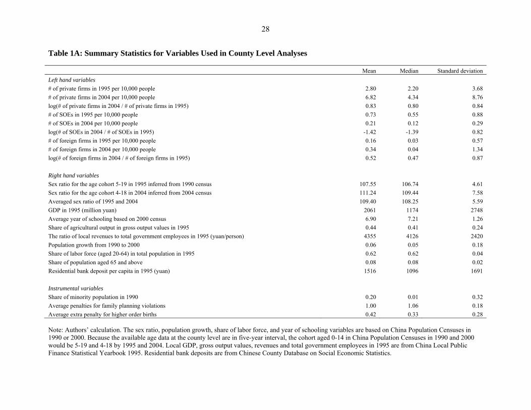
28

Table 1A: Summary Statistics for Variables Used in County Level Analyses Mean Median Standard deviation Left hand variables      

# of private firms in 1995 per 10,000 people 2.80 2.20 3.68 # of private firms in 2004 per 10,000 people 6.82 4.34 8.76 log(# of private firms in 2004 / # of private firms in 1995) 0.83 0.80 0.84 # of SOEs in 1995 per 10,000 people 0.73 0.55 0.88 # of SOEs in 2004 per 10,000 people 0.21 0.12 0.29 log(# of SOEs in 2004 / # of SOEs in 1995) -1.42 -1.39 0.82 # of foreign firms in 1995 per 10,000 people 0.16 0.03 0.57 # of foreign firms in 2004 per 10,000 people 0.34 0.04 1.34 log(# of foreign firms in 2004 / # of foreign firms in 1995) 0.52 0.47 0.87 Right hand variables      

Sex ratio for the age cohort 5-19 in 1995 inferred from 1990 census 107.55 106.74 4.61 Sex ratio for the age cohort 4-18 in 2004 inferred from 2004 census 111.24 109.44 7.58 Averaged sex ratio of 1995 and 2004 109.40 108.25 5.59 GDP in 1995 (million yuan) 2061 1174 2748 Average year of schooling based on 2000 census 6.90 7.21 1.26 Share of agricultural output in gross output values in 1995 0.44 0.41 0.24 The ratio of local revenues to total government employees in 1995 (yuan/person) 4355 4126 2420 Population growth from 1990 to 2000 0.06 0.05 0.18 Share of labor force (aged 20-64) in total population in 1995 0.62 0.62 0.04 Share of population aged 65 and above 0.08 0.08 0.02 Residential bank deposit per capita in 1995 (yuan) 1516 1096 1691        

Instrumental variables      

Share of minority population in 1990 0.20 0.01 0.32 Average penalties for family planning violations 1.00 1.06 0.18 Average extra penalty for higher order births 0.42 0.33 0.28 Note: Authors’ calculation. The sex ratio, population growth, share of labor force, and year of schooling variables are based on China Population Censuses in 1990 or 2000. Because the available age data at the county level are in five-year interval, the cohort aged 0-14 in China Population Censuses in 1990 and 2000 would be 5-19 and 4-18 by 1995 and 2004. Local GDP, gross output values, revenues and total government employees in 1995 are from China Local Public Finance Statistical Yearbook 1995. Residential bank deposits are from Chinese County Database on Social Economic Statistics.

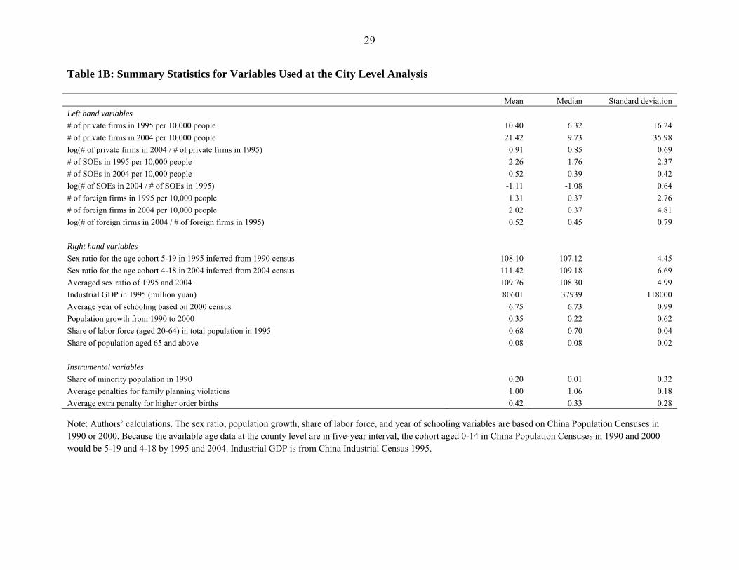
29

Table 1B: Summary Statistics for Variables Used at the City Level Analysis   Mean Median Standard deviation Left hand variables      

# of private firms in 1995 per 10,000 people 10.40 6.32 16.24 # of private firms in 2004 per 10,000 people 21.42 9.73 35.98 log(# of private firms in 2004 / # of private firms in 1995) 0.91 0.85 0.69 # of SOEs in 1995 per 10,000 people 2.26 1.76 2.37 # of SOEs in 2004 per 10,000 people 0.52 0.39 0.42 log(# of SOEs in 2004 / # of SOEs in 1995) -1.11 -1.08 0.64 # of foreign firms in 1995 per 10,000 people 1.31 0.37 2.76 # of foreign firms in 2004 per 10,000 people 2.02 0.37 4.81 log(# of foreign firms in 2004 / # of foreign firms in 1995) 0.52 0.45 0.79 Right hand variables      

Sex ratio for the age cohort 5-19 in 1995 inferred from 1990 census 108.10 107.12 4.45 Sex ratio for the age cohort 4-18 in 2004 inferred from 2004 census 111.42 109.18 6.69 Averaged sex ratio of 1995 and 2004 109.76 108.30 4.99 Industrial GDP in 1995 (million yuan) 80601 37939 118000 Average year of schooling based on 2000 census 6.75 6.73 0.99 Population growth from 1990 to 2000 0.35 0.22 0.62 Share of labor force (aged 20-64) in total population in 1995 0.68 0.70 0.04 Share of population aged 65 and above 0.08 0.08 0.02        

Instrumental variables      

Share of minority population in 1990 0.20 0.01 0.32 Average penalties for family planning violations 1.00 1.06 0.18 Average extra penalty for higher order births 0.42 0.33 0.28 Note: Authors’ calculations. The sex ratio, population growth, share of labor force, and year of schooling variables are based on China Population Censuses in 1990 or 2000. Because the available age data at the county level are in five-year interval, the cohort aged 0-14 in China Population Censuses in 1990 and 2000 would be 5-19 and 4-18 by 1995 and 2004. Industrial GDP is from China Industrial Census 1995.

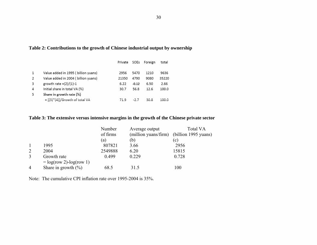
30

 

 Table 2: Contributions to the growth of Chinese industrial output by ownership  

  Table 3: The extensive versus intensive margins in the growth of the Chinese private sector Number Average output Total VA

of firms (million yuans/firm) (billion 1995 yuans) (a) (b) (c) 1 1995 807821 3.66 2956 2 2004 2549888 6.20 15815 3 Growth rate 0.499 0.229 0.728 = log(row 2)-log(row 1) 4 Share in growth (%) 68.5 31.5 100 Note: The cumulative CPI inflation rate over 1995-2004 is 35%.  

31

 Table 4: Sex Ratios and the Growth in the Number of Private Firms at the County Level from 1995 to 2004 Sex ratio for the age cohort in 1995 Sex ratio for the average age cohort between 1995 and 2004 5-19 5-19 5-9 10-14 15-19 5-19 5-19 5-9 10-14 15-19 Initial sex ratio 0.017** 0.016** 0.008** 0.012** 0.007 0.021** 0.020** 0.015** 0.019** 0.014** (0.00) (0.00) (0.00) (0.00) (0.01) (0.00) (0.00) (0.00) (0.00) (0.01) Log number of firms in 1995 -0.493** -0.497** -0.489** -0.493** -0.484** -0.518** -0.518** -0.530** -0.523** -0.491** (0.03) (0.03) (0.03) (0.03) (0.03) (0.03) (0.03) (0.03) (0.03) (0.03) Log GDP in 1995 0.267** 0.272** 0.264** 0.272** 0.273** 0.261** 0.267** 0.258** 0.261** 0.270** (0.04) (0.05) (0.04) (0.05) (0.05) (0.04) (0.05) (0.04) (0.04) (0.05) Average year of schooling based on 1990 census -0.070** -0.086** -0.072** -0.071** -0.075** -0.056* -0.078** -0.063** -0.056* -0.064** (0.03) (0.03) (0.03) (0.03) (0.03) (0.03) (0.03) (0.03) (0.03) (0.03) Share of agricultural output in gross output values in 1995 -0.911** -0.915** -0.929** -0.913** -0.909** -0.915** -0.909** -0.930** -0.917** -0.905** (0.12) (0.12) (0.12) (0.12) (0.12) (0.12) (0.12) (0.12) (0.12) (0.12) The ratio of local revenues to total government employees (log) in 1995 0.073* 0.064 0.075* 0.072* 0.072* 0.069* 0.056 0.073* 0.067* 0.070* (0.04) (0.04) (0.04) (0.04) (0.04) (0.04) (0.04) (0.04) (0.04) (0.04) Population growth from 1990 to 2000 0.428** 0.446** 0.430** 0.424** 0.413** 0.426** 0.431** 0.415** 0.427** 0.420** (0.10) (0.11) (0.10) (0.10) (0.10) (0.09) (0.11) (0.09) (0.09) (0.10) Share of labor force (aged 20-64) in total population in 1995 -0.024 -0.039 -0.169 0.025 -0.012 0.569 0.472 0.963* 0.801 0.054 (0.49) (0.51) (0.50) (0.50) (0.51) (0.50) (0.51) (0.50) (0.51) (0.50) Share of population aged 65 and above in total population in 1995 11.174** 11.210** 11.351** 11.193** 11.165** 11.868** 11.846** 12.092** 12.098** 11.345** (1.36) (1.37) (1.36) (1.36) (1.37) (1.36) (1.37) (1.35) (1.36) (1.37) Dummy for coastal provinces 0.248** 0.255** 0.245** 0.259** 0.261** 0.263** 0.261** 0.268** 0.267** 0.262** (0.04) (0.05) (0.04) (0.04) (0.04) (0.04) (0.05) (0.04) (0.04) (0.04) Log local household savings per capita in 1995 0.00 0.015 (0.04) (0.04) Adjusted R square 0.33 0.33 0.33 0.33 0.32 0.34 0.34 0.35 0.34 0.33 AIC 3753 3693 3754 3764 3772 3729 3671 3711 3724 3764 N 1790 1764 1790 1790 1790 1790 1764 1790 1790 1790 Notes: The growth in the number of private firms is measured by the increase in the log number of firms from 1995 to 2004. The definition of private firms includes township-and-village enterprises and other “collectively owned” firms. The sex ratio for the age cohort 5-19 in 1995 is inferred from the age cohort 0-14 in the 1990 population census; the sex ratio for the age cohort 4-18 in 2004 is inferred from the age cohort 0-14 in the 2000 population census. Local household savings is measured by residential bank deposits. Robust standard errors are in parentheses. * and ** denote statistically significant at the 10% and 5% levels, respectively.

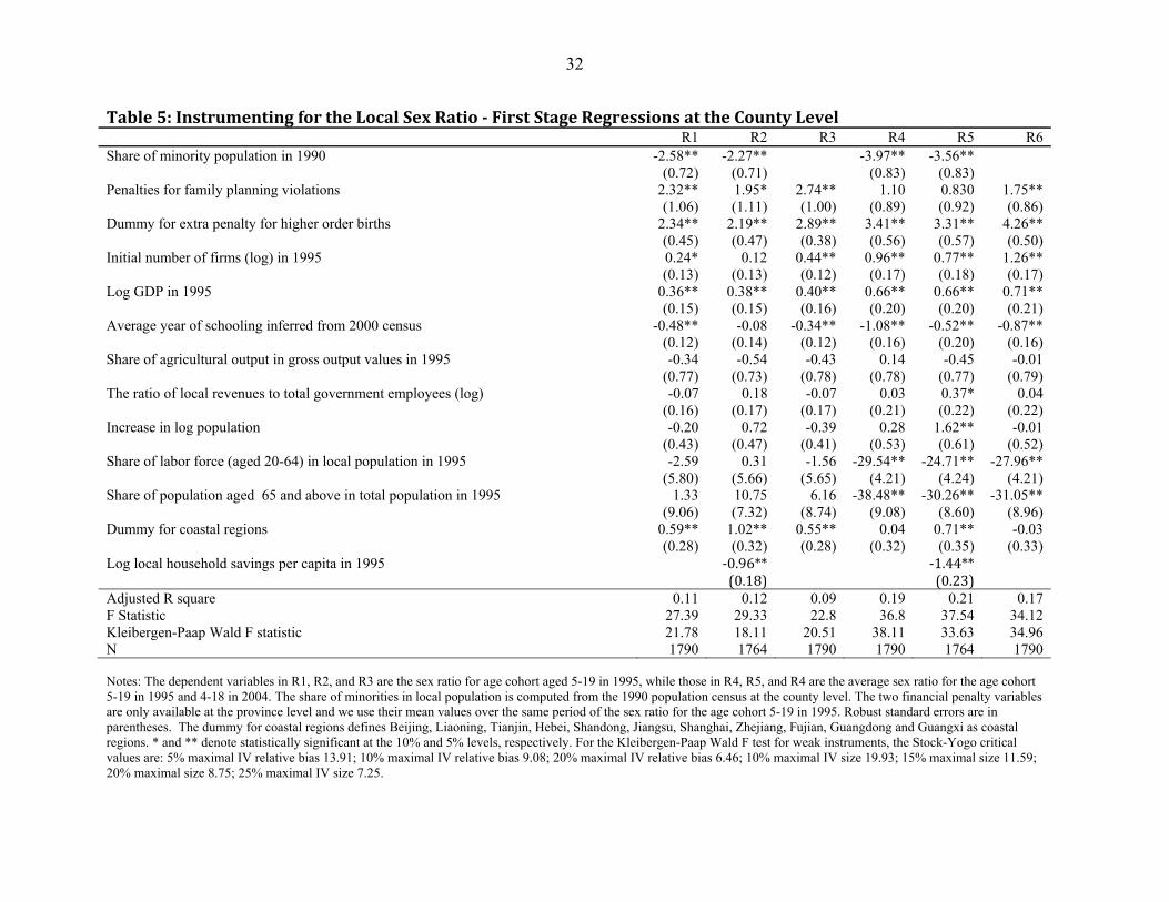
32

Table 5: Instrumenting for the Local Sex Ratio ­ First Stage Regressions at the County Level R1 R2 R3 R4 R5 R6 Share of minority population in 1990 -2.58** -2.27** -3.97** -3.56** (0.72) (0.71) (0.83) (0.83) Penalties for family planning violations 2.32** 1.95* 2.74** 1.10 0.830 1.75** (1.06) (1.11) (1.00) (0.89) (0.92) (0.86) Dummy for extra penalty for higher order births 2.34** 2.19** 2.89** 3.41** 3.31** 4.26** (0.45) (0.47) (0.38) (0.56) (0.57) (0.50) Initial number of firms (log) in 1995 0.24* 0.12 0.44** 0.96** 0.77** 1.26** (0.13) (0.13) (0.12) (0.17) (0.18) (0.17) Log GDP in 1995 0.36** 0.38** 0.40** 0.66** 0.66** 0.71** (0.15) (0.15) (0.16) (0.20) (0.20) (0.21) Average year of schooling inferred from 2000 census -0.48** -0.08 -0.34** -1.08** -0.52** -0.87** (0.12) (0.14) (0.12) (0.16) (0.20) (0.16) Share of agricultural output in gross output values in 1995 -0.34 -0.54 -0.43 0.14 -0.45 -0.01 (0.77) (0.73) (0.78) (0.78) (0.77) (0.79) The ratio of local revenues to total government employees (log) -0.07 0.18 -0.07 0.03 0.37* 0.04 (0.16) (0.17) (0.17) (0.21) (0.22) (0.22) Increase in log population -0.20 0.72 -0.39 0.28 1.62** -0.01 (0.43) (0.47) (0.41) (0.53) (0.61) (0.52) Share of labor force (aged 20-64) in local population in 1995 -2.59 0.31 -1.56 -29.54** -24.71** -27.96** (5.80) (5.66) (5.65) (4.21) (4.24) (4.21) Share of population aged 65 and above in total population in 1995 1.33 10.75 6.16 -38.48** -30.26** -31.05** (9.06) (7.32) (8.74) (9.08) (8.60) (8.96) Dummy for coastal regions 0.59** 1.02** 0.55** 0.04 0.71** -0.03 (0.28) (0.32) (0.28) (0.32) (0.35) (0.33) Log local household savings per capita in 1995   ‐0.96** ‐1.44**    (0.18) (0.23)   Adjusted R square 0.11 0.12 0.09 0.19 0.21 0.17 F Statistic 27.39 29.33 22.8 36.8 37.54 34.12 Kleibergen-Paap Wald F statistic 21.78 18.11 20.51 38.11 33.63 34.96 N 1790 1764 1790 1790 1764 1790 Notes: The dependent variables in R1, R2, and R3 are the sex ratio for age cohort aged 5-19 in 1995, while those in R4, R5, and R4 are the average sex ratio for the age cohort 5-19 in 1995 and 4-18 in 2004. The share of minorities in local population is computed from the 1990 population census at the county level. The two financial penalty variables are only available at the province level and we use their mean values over the same period of the sex ratio for the age cohort 5-19 in 1995. Robust standard errors are in parentheses. The dummy for coastal regions defines Beijing, Liaoning, Tianjin, Hebei, Shandong, Jiangsu, Shanghai, Zhejiang, Fujian, Guangdong and Guangxi as coastal regions. * and ** denote statistically significant at the 10% and 5% levels, respectively. For the Kleibergen-Paap Wald F test for weak instruments, the Stock-Yogo critical values are: 5% maximal IV relative bias 13.91; 10% maximal IV relative bias 9.08; 20% maximal IV relative bias 6.46; 10% maximal IV size 19.93; 15% maximal size 11.59; 20% maximal size 8.75; 25% maximal IV size 7.25.

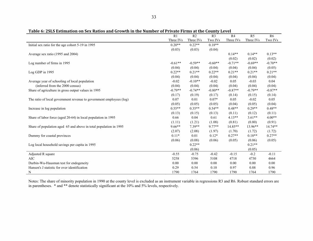
33

Table 6: 2SLS Estimation on Sex Ratios and Growth in the Number of Private Firms at the County Level 

R1

Three IVs R2

Three IVs R3

Two IVs R4

Three IVs R5

Three IVs R6

Two IVs Initial sex ratio for the age cohort 5-19 in 1995 0.20** 0.22** 0.18** (0.03) (0.03) (0.04) Average sex ratio (1995 and 2004) 0.14** 0.14** 0.13** (0.02) (0.02) (0.02) Log number of firms in 1995 -0.61** -0.59** -0.60** -0.71** -0.69** -0.70** (0.04) (0.04) (0.04) (0.04) (0.04) (0.05) Log GDP in 1995 0.22** 0.21** 0.22** 0.21** 0.21** 0.21** (0.04) (0.04) (0.04) (0.04) (0.04) (0.04) Average year of schooling of local population -0.02 -0.10** -0.02 0.05 -0.03 0.04 (inferred from the 2000 census) (0.04) (0.04) (0.04) (0.04) (0.04) (0.04) Share of agriculture in gross output values in 1995 -0.79** -0.74** -0.80** -0.87** -0.79** -0.87** (0.17) (0.19) (0.17) (0.14) (0.15) (0.14) The ratio of local government revenue to government employees (log) 0.07 0.01 0.07* 0.05 -0.02 0.05 (0.05) (0.05) (0.05) (0.04) (0.05) (0.04) Increase in log population 0.55** 0.35** 0.54** 0.48** 0.29** 0.48** (0.13) (0.15) (0.13) (0.11) (0.12) (0.11) Share of labor force (aged 20-64) in local population in 1995 0.66 0.04 0.61 4.13** 3.61** 4.00** (1.11) (1.21) (1.08) (0.81) (0.80) (0.91) Share of population aged 65 and above in total population in 1995 9.66** 7.39** 9.77** 14.85** 13.96** 14.74** (2.07) (2.08) (1.97) (1.70) (1.72) (1.72) Dummy for coastal provinces 0.11* 0.01 0.12* 0.27** 0.18** 0.27** (0.06) (0.08) (0.06) (0.05) (0.06) (0.05) Log local household savings per capita in 1995 0.22** 0.21** (0.06) (0.05) Adjusted R square -0.55 -0.75 -0.42 -0.15 -0.2 -0.11 AIC 5258 5396 5108 4718 4730 4664 Durbin-Wu-Hausman test for endogeneity 0.00 0.00 0.00 0.00 0.00 0.00 Hansen's J statistic for over identification 0.29 0.54 0.10 0.97 0.88 0.96 N 1790 1764 1790 1790 1764 1790 Notes: The share of minority population in 1990 at the county level is excluded as an instrument variable in regressions R3 and R6. Robust standard errors are in parentheses. * and ** denote statistically significant at the 10% and 5% levels, respectively.

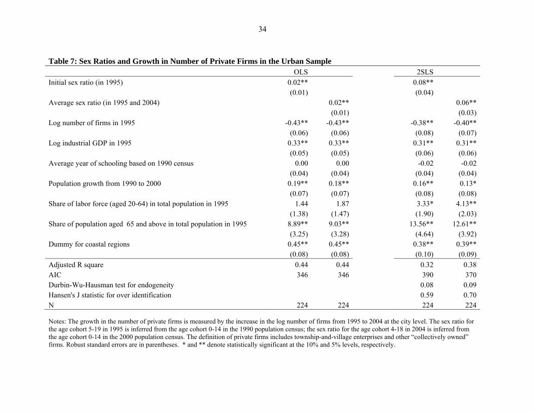
34

Table 7: Sex Ratios and Growth in Number of Private Firms in the Urban Sample OLS 2SLS Initial sex ratio (in 1995) 0.02** 0.08** (0.01) (0.04)Average sex ratio (in 1995 and 2004) 0.02** 0.06** (0.01) (0.03)Log number of firms in 1995 -0.43** -0.43** -0.38** -0.40** (0.06) (0.06) (0.08) (0.07)Log industrial GDP in 1995 0.33** 0.33** 0.31** 0.31** (0.05) (0.05) (0.06) (0.06)Average year of schooling based on 1990 census 0.00 0.00 -0.02 -0.02 (0.04) (0.04) (0.04) (0.04)Population growth from 1990 to 2000 0.19** 0.18** 0.16** 0.13* (0.07) (0.07) (0.08) (0.08)Share of labor force (aged 20-64) in total population in 1995 1.44 1.87 3.33* 4.13** (1.38) (1.47) (1.90) (2.03)Share of population aged 65 and above in total population in 1995 8.89** 9.03** 13.56** 12.61** (3.25) (3.28) (4.64) (3.92)Dummy for coastal regions 0.45** 0.45** 0.38** 0.39** (0.08) (0.08) (0.10) (0.09)Adjusted R square 0.44 0.44 0.32 0.38AIC 346 346 390 370Durbin-Wu-Hausman test for endogeneity 0.08 0.09Hansen's J statistic for over identification 0.59 0.70N 224 224 224 224 Notes: The growth in the number of private firms is measured by the increase in the log number of firms from 1995 to 2004 at the city level. The sex ratio for the age cohort 5-19 in 1995 is inferred from the age cohort 0-14 in the 1990 population census; the sex ratio for the age cohort 4-18 in 2004 is inferred from the age cohort 0-14 in the 2000 population census. The definition of private firms includes township-and-village enterprises and other “collectively owned” firms. Robust standard errors are in parentheses. * and ** denote statistically significant at the 10% and 5% levels, respectively.

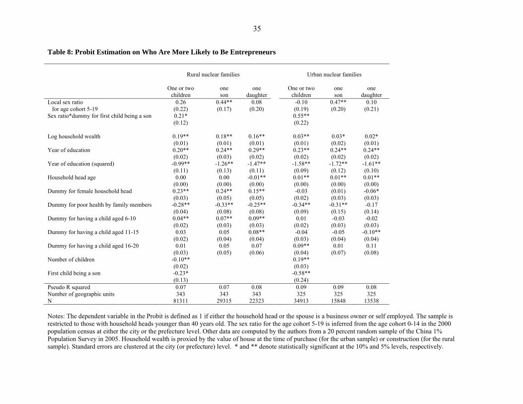
35

Table 8: Probit Estimation on Who Are More Likely to Be Entrepreneurs

Rural nuclear families

Urban nuclear families

One or two

children one son

one daughter

One or two children

one son

one daughter

Local sex ratio 0.26 0.44** 0.08 -0.10 0.47** 0.10 for age cohort 5-19 (0.22) (0.17) (0.20) (0.19) (0.20) (0.21) Sex ratio*dummy for first child being a son 0.21* 0.55**

(0.12)

(0.22)

Log household wealth 0.19** 0.18** 0.16** 0.03** 0.03* 0.02* (0.01) (0.01) (0.01) (0.01) (0.02) (0.01) Year of education 0.20** 0.24** 0.29** 0.23** 0.24** 0.24** (0.02) (0.03) (0.02) (0.02) (0.02) (0.02) Year of education (squared) -0.99** -1.26** -1.47** -1.58** -1.72** -1.61** (0.11) (0.13) (0.11) (0.09) (0.12) (0.10) Household head age 0.00 0.00 -0.01** 0.01** 0.01** 0.01** (0.00) (0.00) (0.00) (0.00) (0.00) (0.00) Dummy for female household head 0.23** 0.24** 0.15** -0.03 (0.01) -0.06* (0.03) (0.05) (0.05) (0.02) (0.03) (0.03) Dummy for poor health by family members -0.28** -0.33** -0.25** -0.34** -0.31** -0.17 (0.04) (0.08) (0.08) (0.09) (0.15) (0.14) Dummy for having a child aged 6-10 0.04** 0.07** 0.09** 0.01 -0.03 -0.02 (0.02) (0.03) (0.03) (0.02) (0.03) (0.03) Dummy for having a child aged 11-15 0.03 0.05 0.08** -0.04 -0.05 -0.10** (0.02) (0.04) (0.04) (0.03) (0.04) (0.04) Dummy for having a child aged 16-20 0.01 0.05 0.07 0.09** 0.01 0.11 (0.03) (0.05) (0.06) (0.04) (0.07) (0.08) Number of children -0.10** 0.19** (0.02) (0.03) First child being a son -0.23* -0.58** (0.13) (0.24) Pseudo R squared 0.07 0.07 0.08 0.09 0.09 0.08 Number of geographic units 343 343 343 325 325 325 N 81311 29315 22323 34913 15848 13538 Notes: The dependent variable in the Probit is defined as 1 if either the household head or the spouse is a business owner or self employed. The sample is restricted to those with household heads younger than 40 years old. The sex ratio for the age cohort 5-19 is inferred from the age cohort 0-14 in the 2000 population census at either the city or the prefecture level. Other data are computed by the authors from a 20 percent random sample of the China 1% Population Survey in 2005. Household wealth is proxied by the value of house at the time of purchase (for the urban sample) or construction (for the rural sample). Standard errors are clustered at the city (or prefecture) level. * and ** denote statistically significant at the 10% and 5% levels, respectively.

36

Table 9: Placebo Tests the Growth in the Number of Foreign-invested Firms at the County Level OLS 2SLS R1 R2 R3 R4 R5 R6 Sex ratio for the age cohort 5-19 in 1995 0.00 -0.01 (0.01) (0.03) Sex ratio for the cohort 5-19 averaged over 1995 and 2004 0.01 0.01 0.00 0.01 (0.00) (0.00) (0.02) (0.02) Log number of firms in 1995 -0.30** -0.30** -0.31** -0.30** -0.30** -0.31** (0.03) (0.03) (0.03) (0.03) (0.03) (0.03) Log GDP in 1995 0.13** 0.13** 0.13** 0.14** 0.13** 0.13** (0.05) (0.05) (0.05) (0.05) (0.05) (0.05) Average year of schooling based on 2000 census -0.04 -0.03 -0.08 -0.05 -0.04 -0.08 (0.05) (0.05) (0.05) (0.05) (0.05) (0.05) Share of agricultural output in gross output values in 1995 -0.76** -0.75** -0.72** -0.77** -0.75** -0.72** (0.16) (0.16) (0.16) (0.16) (0.16) (0.17) The ratio of local revenues to total government employees 0.30** 0.30** 0.29** 0.30** 0.30** 0.29** (0.06) (0.06) (0.06) (0.06) (0.06) (0.06) Increase in log population 0.29** 0.29** 0.25 0.29** 0.29** 0.25 (0.14) (0.14) (0.17) (0.14) (0.14) (0.17) Share of labor force (aged 20-64) in local population in 1995 0.80 1.05 0.85 0.72 0.89 0.87 (0.66) (0.69) (0.70) (0.71) (1.03) (1.02) Share of population aged 65 and above in total population in 1995 7.81** 8.08** 7.47** 7.68** 7.91** 7.49** (1.83) (1.86) (1.92) (1.87) (2.05) (2.04) Dummy for coastal regions 0.55** 0.55** 0.53** 0.57** 0.55** 0.53** (0.06) (0.06) (0.06) (0.07) (0.06) (0.06) Log local household savings per capita in 1995 0.07 0.08 (0.06) (0.07) Adjusted R square 0.21 0.21 0.21 0.21 0.21 0.21 AIC 2497 2495 2456 2501 2496 2456 Durbin-Wu-Hausman test for endogeneity 0.74 0.85 0.98 Hansen's J statistic for over identification 0.06 0.06 0.06 Kleibergen-Paap Wald F statistic 19.97 21.69 18.49 N 1071 1071 1053 1071 1071 1053 Notes: Foreign invested firms refer to both wholly foreign owned and Sino-foreign joint ventures. Robust standard errors are in parentheses. * and ** denote statistically significant at the 10% and 5% levels, respectively.

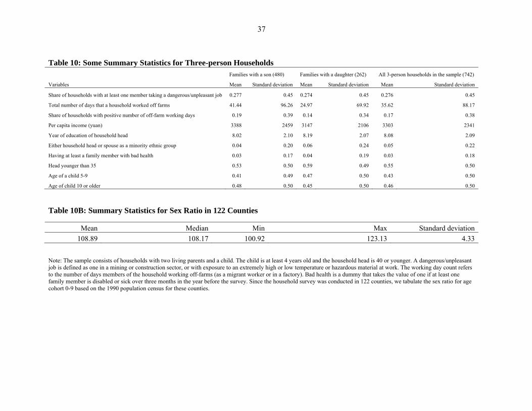
37

  Table 10: Some Summary Statistics for Three-person Households Families with a son (480) Families with a daughter (262) All 3-person households in the sample (742)

Variables Mean Standard deviation Mean Standard deviation Mean Standard deviation

Share of households with at least one member taking a dangerous/unpleasant job 0.277 0.45 0.274 0.45 0.276 0.45

Total number of days that a household worked off farms 41.44 96.26 24.97 69.92 35.62 88.17

Share of households with positive number of off-farm working days 0.19 0.39 0.14 0.34 0.17 0.38

Per capita income (yuan) 3388 2459 3147 2106 3303 2341

Year of education of household head 8.02 2.10 8.19 2.07 8.08 2.09

Either household head or spouse as a minority ethnic group 0.04 0.20 0.06 0.24 0.05 0.22

Having at least a family member with bad health 0.03 0.17 0.04 0.19 0.03 0.18

Head younger than 35 0.53 0.50 0.59 0.49 0.55 0.50

Age of a child 5-9 0.41 0.49 0.47 0.50 0.43 0.50

Age of child 10 or older 0.48 0.50 0.45 0.50 0.46 0.50

  Table 10B: Summary Statistics for Sex Ratio in 122 Counties

Mean Median Min Max Standard deviation108.89 108.17 100.92 123.13 4.33

Note: The sample consists of households with two living parents and a child. The child is at least 4 years old and the household head is 40 or younger. A dangerous/unpleasant job is defined as one in a mining or construction sector, or with exposure to an extremely high or low temperature or hazardous material at work. The working day count refers to the number of days members of the household working off-farms (as a migrant worker or in a factory). Bad health is a dummy that takes the value of one if at least one family member is disabled or sick over three months in the year before the survey. Since the household survey was conducted in 122 counties, we tabulate the sex ratio for age cohort 0-9 based on the 1990 population census for these counties.

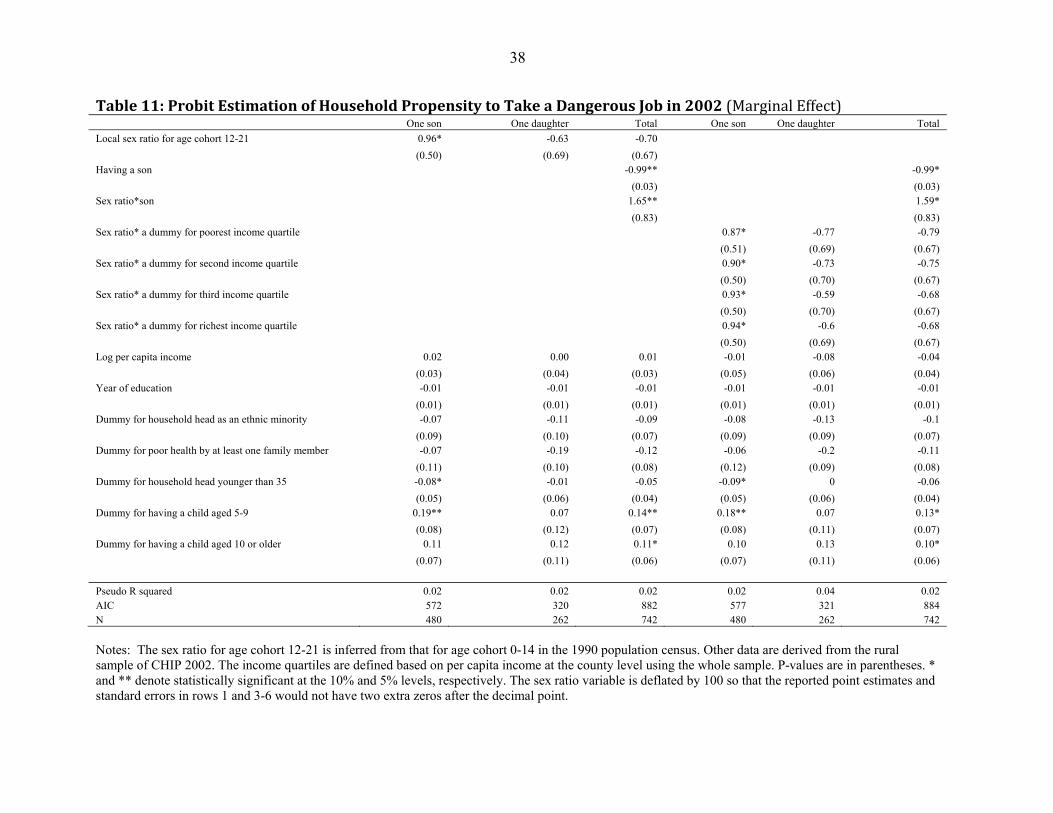
38

Table 11: Probit Estimation of Household Propensity to Take a Dangerous Job in 2002 (Marginal Effect)  One son One daughter Total One son One daughter Total Local sex ratio for age cohort 12-21 0.96* -0.63 -0.70 (0.50) (0.69) (0.67) Having a son -0.99** -0.99* (0.03) (0.03) Sex ratio*son 1.65** 1.59* (0.83) (0.83) Sex ratio* a dummy for poorest income quartile 0.87* -0.77 -0.79 (0.51) (0.69) (0.67) Sex ratio* a dummy for second income quartile 0.90* -0.73 -0.75 (0.50) (0.70) (0.67) Sex ratio* a dummy for third income quartile 0.93* -0.59 -0.68 (0.50) (0.70) (0.67) Sex ratio* a dummy for richest income quartile 0.94* -0.6 -0.68 (0.50) (0.69) (0.67) Log per capita income 0.02 0.00 0.01 -0.01 -0.08 -0.04 (0.03) (0.04) (0.03) (0.05) (0.06) (0.04) Year of education -0.01 -0.01 -0.01 -0.01 -0.01 -0.01 (0.01) (0.01) (0.01) (0.01) (0.01) (0.01) Dummy for household head as an ethnic minority -0.07 -0.11 -0.09 -0.08 -0.13 -0.1 (0.09) (0.10) (0.07) (0.09) (0.09) (0.07) Dummy for poor health by at least one family member -0.07 -0.19 -0.12 -0.06 -0.2 -0.11 (0.11) (0.10) (0.08) (0.12) (0.09) (0.08) Dummy for household head younger than 35 -0.08* -0.01 -0.05 -0.09* 0 -0.06 (0.05) (0.06) (0.04) (0.05) (0.06) (0.04) Dummy for having a child aged 5-9 0.19** 0.07 0.14** 0.18** 0.07 0.13* (0.08) (0.12) (0.07) (0.08) (0.11) (0.07) Dummy for having a child aged 10 or older 0.11 0.12 0.11* 0.10 0.13 0.10* (0.07) (0.11) (0.06) (0.07) (0.11) (0.06) Pseudo R squared 0.02 0.02 0.02 0.02 0.04 0.02 AIC 572 320 882 577 321 884 N 480 262 742 480 262 742 Notes: The sex ratio for age cohort 12-21 is inferred from that for age cohort 0-14 in the 1990 population census. Other data are derived from the rural sample of CHIP 2002. The income quartiles are defined based on per capita income at the county level using the whole sample. P-values are in parentheses. * and ** denote statistically significant at the 10% and 5% levels, respectively. The sex ratio variable is deflated by 100 so that the reported point estimates and standard errors in rows 1 and 3-6 would not have two extra zeros after the decimal point.

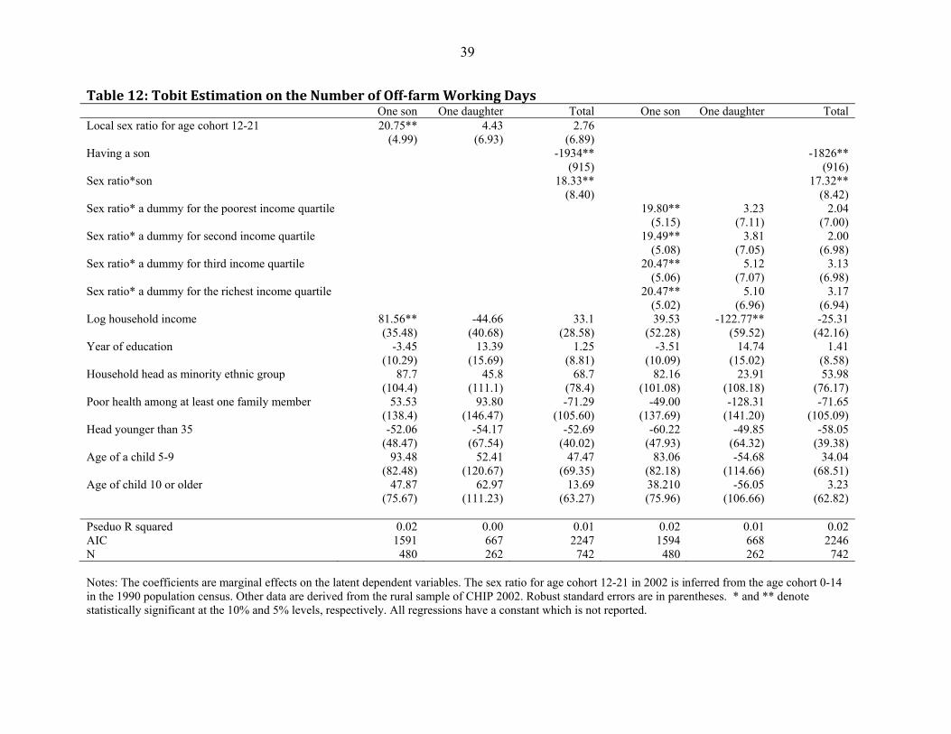
39

Table 12: Tobit Estimation on the Number of Off­farm Working Days One son One daughter Total One son One daughter Total Local sex ratio for age cohort 12-21 20.75** 4.43 2.76 (4.99) (6.93) (6.89) Having a son -1934** -1826** (915) (916) Sex ratio*son 18.33** 17.32** (8.40) (8.42) Sex ratio* a dummy for the poorest income quartile 19.80** 3.23 2.04 (5.15) (7.11) (7.00) Sex ratio* a dummy for second income quartile 19.49** 3.81 2.00 (5.08) (7.05) (6.98) Sex ratio* a dummy for third income quartile 20.47** 5.12 3.13 (5.06) (7.07) (6.98) Sex ratio* a dummy for the richest income quartile 20.47** 5.10 3.17 (5.02) (6.96) (6.94) Log household income 81.56** -44.66 33.1 39.53 -122.77** -25.31 (35.48) (40.68) (28.58) (52.28) (59.52) (42.16) Year of education -3.45 13.39 1.25 -3.51 14.74 1.41 (10.29) (15.69) (8.81) (10.09) (15.02) (8.58) Household head as minority ethnic group 87.7 45.8 68.7 82.16 23.91 53.98 (104.4) (111.1) (78.4) (101.08) (108.18) (76.17) Poor health among at least one family member 53.53 93.80 -71.29 -49.00 -128.31 -71.65 (138.4) (146.47) (105.60) (137.69) (141.20) (105.09) Head younger than 35 -52.06 -54.17 -52.69 -60.22 -49.85 -58.05 (48.47) (67.54) (40.02) (47.93) (64.32) (39.38) Age of a child 5-9 93.48 52.41 47.47 83.06 -54.68 34.04 (82.48) (120.67) (69.35) (82.18) (114.66) (68.51) Age of child 10 or older 47.87 62.97 13.69 38.210 -56.05 3.23 (75.67) (111.23) (63.27) (75.96) (106.66) (62.82) Pseduo R squared 0.02 0.00 0.01 0.02 0.01 0.02 AIC 1591 667 2247 1594 668 2246 N 480 262 742 480 262 742 Notes: The coefficients are marginal effects on the latent dependent variables. The sex ratio for age cohort 12-21 in 2002 is inferred from the age cohort 0-14 in the 1990 population census. Other data are derived from the rural sample of CHIP 2002. Robust standard errors are in parentheses. * and ** denote statistically significant at the 10% and 5% levels, respectively. All regressions have a constant which is not reported.

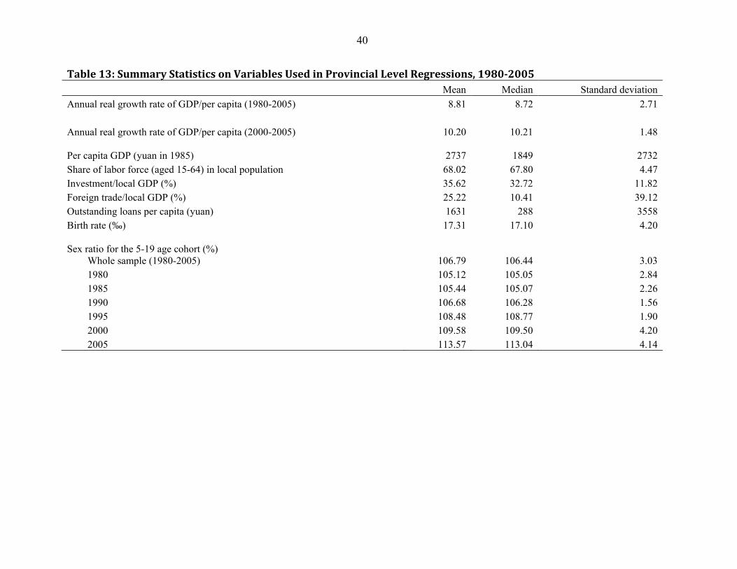
40

Table 13: Summary Statistics on Variables Used in Provincial Level Regressions, 1980­2005 Mean Median Standard deviationAnnual real growth rate of GDP/per capita (1980-2005) 8.81 8.72 2.71 Annual real growth rate of GDP/per capita (2000-2005) 10.20 10.21 1.48 Per capita GDP (yuan in 1985) 2737 1849 2732Share of labor force (aged 15-64) in local population 68.02 67.80 4.47Investment/local GDP (%) 35.62 32.72 11.82Foreign trade/local GDP (%) 25.22 10.41 39.12Outstanding loans per capita (yuan) 1631 288 3558Birth rate (‰) 17.31 17.10 4.20 Sex ratio for the 5-19 age cohort (%) Whole sample (1980-2005) 106.79 106.44 3.03

1980 105.12 105.05 2.841985 105.44 105.07 2.261990 106.68 106.28 1.561995 108.48 108.77 1.902000 109.58 109.50 4.202005 113.57 113.04 4.14

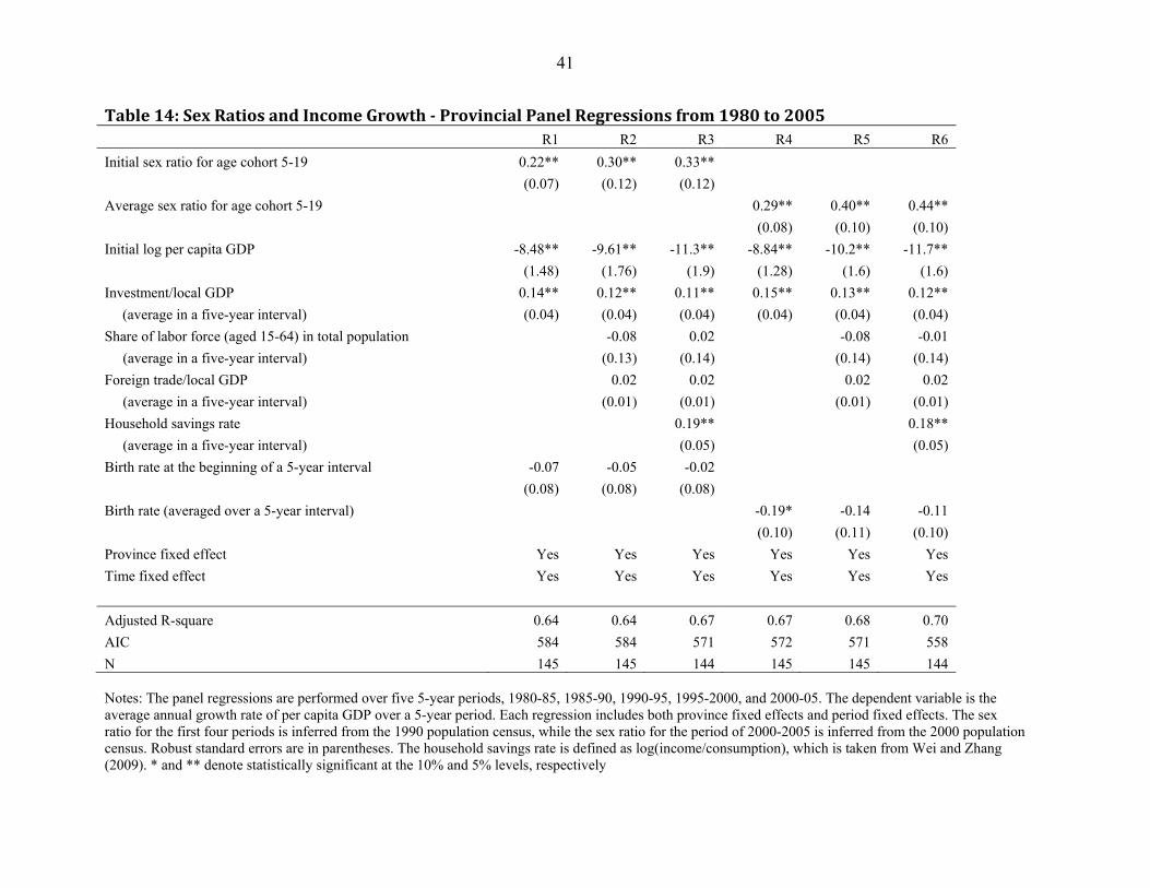
41

Table 14: Sex Ratios and Income Growth ­ Provincial Panel Regressions from 1980 to 2005 R1 R2 R3 R4 R5 R6 Initial sex ratio for age cohort 5-19 0.22** 0.30** 0.33** (0.07) (0.12) (0.12) Average sex ratio for age cohort 5-19 0.29** 0.40** 0.44** (0.08) (0.10) (0.10) Initial log per capita GDP -8.48** -9.61** -11.3** -8.84** -10.2** -11.7**   (1.48) (1.76) (1.9) (1.28) (1.6) (1.6) Investment/local GDP 0.14** 0.12** 0.11** 0.15** 0.13** 0.12**      (average in a five-year interval)  (0.04) (0.04) (0.04) (0.04) (0.04) (0.04) Share of labor force (aged 15-64) in total population -0.08 0.02 -0.08 -0.01 (average in a five-year interval) (0.13) (0.14) (0.14) (0.14) Foreign trade/local GDP 0.02 0.02 0.02 0.02 (average in a five-year interval) (0.01) (0.01) (0.01) (0.01) Household savings rate 0.19** 0.18** (average in a five-year interval) (0.05) (0.05) Birth rate at the beginning of a 5-year interval -0.07 -0.05 -0.02 (0.08) (0.08) (0.08) Birth rate (averaged over a 5-year interval) -0.19* -0.14 -0.11 (0.10) (0.11) (0.10) Province fixed effect Yes Yes Yes Yes Yes Yes Time fixed effect Yes Yes Yes Yes Yes Yes Adjusted R-square 0.64 0.64 0.67 0.67 0.68 0.70 AIC 584 584 571 572 571 558 N 145 145 144 145 145 144 Notes: The panel regressions are performed over five 5-year periods, 1980-85, 1985-90, 1990-95, 1995-2000, and 2000-05. The dependent variable is the average annual growth rate of per capita GDP over a 5-year period. Each regression includes both province fixed effects and period fixed effects. The sex ratio for the first four periods is inferred from the 1990 population census, while the sex ratio for the period of 2000-2005 is inferred from the 2000 population census. Robust standard errors are in parentheses. The household savings rate is defined as log(income/consumption), which is taken from Wei and Zhang (2009). * and ** denote statistically significant at the 10% and 5% levels, respectively

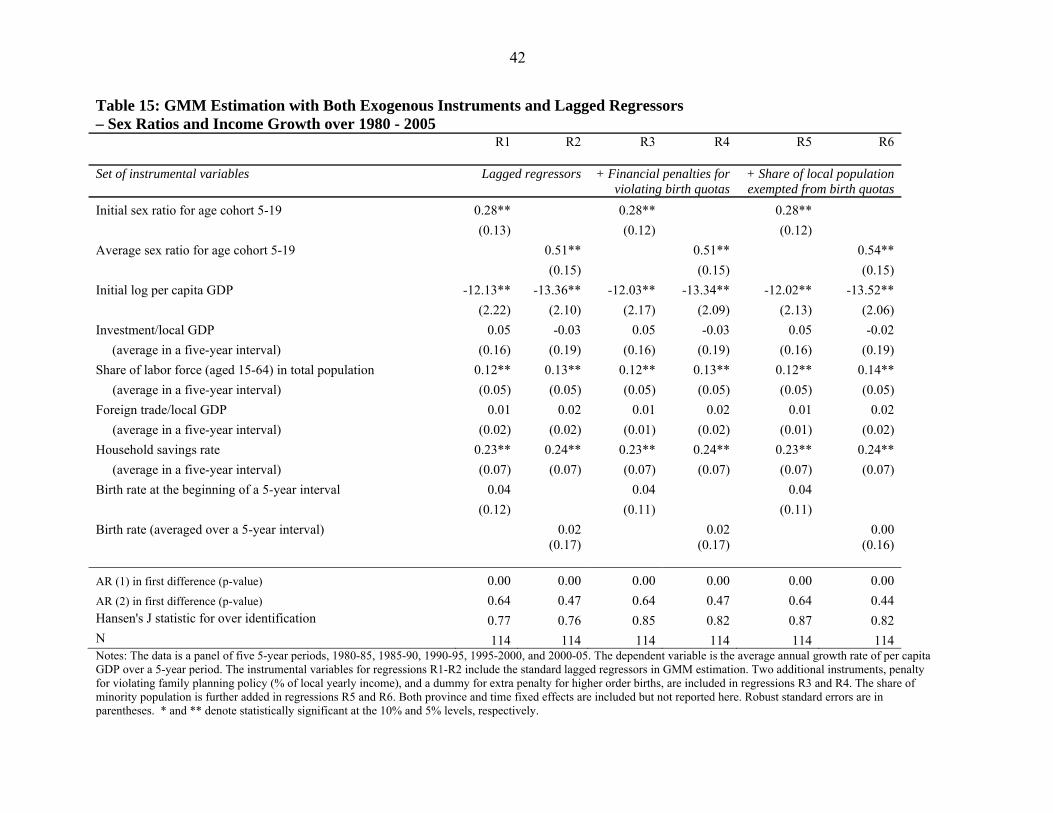
42

Table 15: GMM Estimation with Both Exogenous Instruments and Lagged Regressors – Sex Ratios and Income Growth over 1980 - 2005

R1

R2

R3

R4

R5

R6

Set of instrumental variables

Lagged regressors

+ Financial penalties for violating birth quotas

+ Share of local population exempted from birth quotas

Initial sex ratio for age cohort 5-19 0.28** 0.28** 0.28** (0.13) (0.12) (0.12) Average sex ratio for age cohort 5-19 0.51** 0.51** 0.54** (0.15) (0.15) (0.15) Initial log per capita GDP -12.13** -13.36** -12.03** -13.34** -12.02** -13.52**   (2.22) (2.10) (2.17) (2.09) (2.13) (2.06) Investment/local GDP 0.05 -0.03 0.05 -0.03 0.05 -0.02      (average in a five-year interval)  (0.16) (0.19) (0.16) (0.19) (0.16) (0.19) Share of labor force (aged 15-64) in total population 0.12** 0.13** 0.12** 0.13** 0.12** 0.14** (average in a five-year interval) (0.05) (0.05) (0.05) (0.05) (0.05) (0.05) Foreign trade/local GDP 0.01 0.02 0.01 0.02 0.01 0.02 (average in a five-year interval) (0.02) (0.02) (0.01) (0.02) (0.01) (0.02) Household savings rate 0.23** 0.24** 0.23** 0.24** 0.23** 0.24** (average in a five-year interval) (0.07) (0.07) (0.07) (0.07) (0.07) (0.07) Birth rate at the beginning of a 5-year interval 0.04 0.04 0.04 (0.12) (0.11) (0.11) Birth rate (averaged over a 5-year interval) 0.02 0.02 0.00

(0.17)

(0.17)

(0.16)

AR (1) in first difference (p-value) 0.00 0.00 0.00 0.00 0.00 0.00 AR (2) in first difference (p-value) 0.64 0.47 0.64 0.47 0.64 0.44 Hansen's J statistic for over identification 0.77 0.76 0.85 0.82 0.87 0.82 N 114 114 114 114 114 114 Notes: The data is a panel of five 5-year periods, 1980-85, 1985-90, 1990-95, 1995-2000, and 2000-05. The dependent variable is the average annual growth rate of per capita GDP over a 5-year period. The instrumental variables for regressions R1-R2 include the standard lagged regressors in GMM estimation. Two additional instruments, penalty for violating family planning policy (% of local yearly income), and a dummy for extra penalty for higher order births, are included in regressions R3 and R4. The share of minority population is further added in regressions R5 and R6. Both province and time fixed effects are included but not reported here. Robust standard errors are in parentheses. * and ** denote statistically significant at the 10% and 5% levels, respectively.

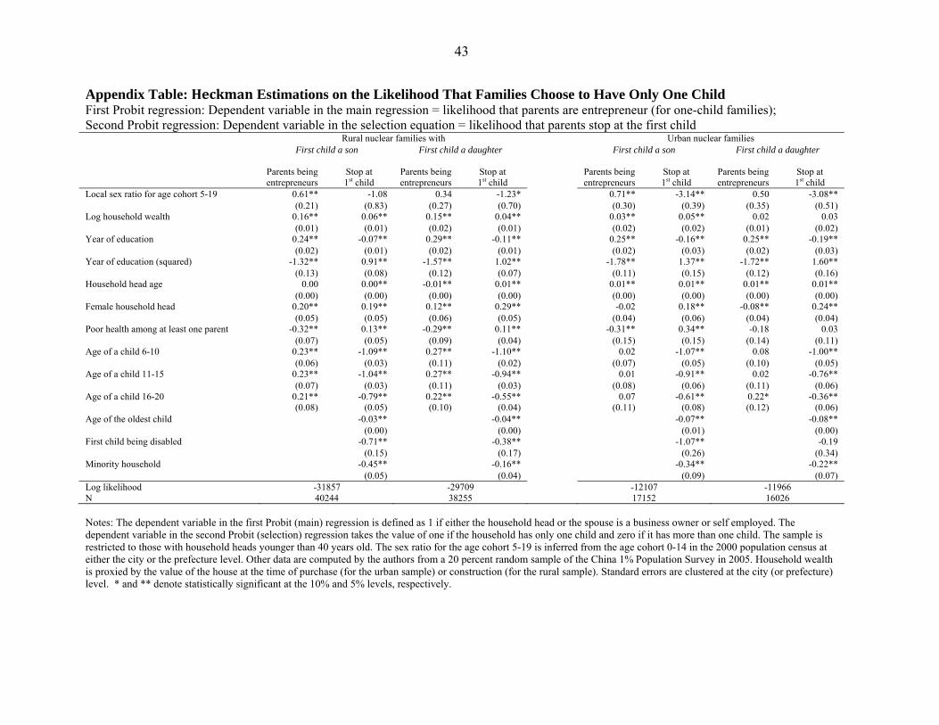
43

Appendix Table: Heckman Estimations on the Likelihood That Families Choose to Have Only One Child First Probit regression: Dependent variable in the main regression = likelihood that parents are entrepreneur (for one-child families); Second Probit regression: Dependent variable in the selection equation = likelihood that parents stop at the first child    Rural nuclear families with Urban nuclear families

 First child a son

First child a daughter   First child a son

First child a daughter

  Parents being entrepreneurs

Stop at 1st child

Parents being entrepreneurs

Stop at 1st child

Parents being entrepreneurs

Stop at 1st child

Parents being entrepreneurs

Stop at 1st child

Local sex ratio for age cohort 5-19 0.61** -1.08 0.34 -1.23* 0.71** -3.14** 0.50 -3.08**   (0.21) (0.83) (0.27) (0.70) (0.30) (0.39) (0.35) (0.51) Log household wealth 0.16** 0.06** 0.15** 0.04** 0.03** 0.05** 0.02 0.03   (0.01) (0.01) (0.02) (0.01) (0.02) (0.02) (0.01) (0.02) Year of education 0.24** -0.07** 0.29** -0.11** 0.25** -0.16** 0.25** -0.19**   (0.02) (0.01) (0.02) (0.01) (0.02) (0.03) (0.02) (0.03) Year of education (squared) -1.32** 0.91** -1.57** 1.02** -1.78** 1.37** -1.72** 1.60**   (0.13) (0.08) (0.12) (0.07) (0.11) (0.15) (0.12) (0.16) Household head age 0.00 0.00** -0.01** 0.01** 0.01** 0.01** 0.01** 0.01**   (0.00) (0.00) (0.00) (0.00) (0.00) (0.00) (0.00) (0.00) Female household head 0.20** 0.19** 0.12** 0.29** -0.02 0.18** -0.08** 0.24**   (0.05) (0.05) (0.06) (0.05) (0.04) (0.06) (0.04) (0.04) Poor health among at least one parent -0.32** 0.13** -0.29** 0.11** -0.31** 0.34** -0.18 0.03   (0.07) (0.05) (0.09) (0.04) (0.15) (0.15) (0.14) (0.11) Age of a child 6-10 0.23** -1.09** 0.27** -1.10** 0.02 -1.07** 0.08 -1.00**   (0.06) (0.03) (0.11) (0.02) (0.07) (0.05) (0.10) (0.05) Age of a child 11-15 0.23** -1.04** 0.27** -0.94** 0.01 -0.91** 0.02 -0.76**   (0.07) (0.03) (0.11) (0.03) (0.08) (0.06) (0.11) (0.06) Age of a child 16-20 0.21** -0.79** 0.22** -0.55** 0.07 -0.61** 0.22* -0.36** (0.08) (0.05) (0.10) (0.04) (0.11) (0.08) (0.12) (0.06) Age of the oldest child -0.03** -0.04** -0.07** -0.08**   (0.00) (0.00) (0.01) (0.00) First child being disabled -0.71** -0.38** -1.07** -0.19   (0.15) (0.17) (0.26) (0.34) Minority household -0.45** -0.16** -0.34** -0.22**   (0.05) (0.04) (0.09) (0.07) Log likelihood -31857 -29709 -12107 -11966 N 40244 38255 17152 16026 Notes: The dependent variable in the first Probit (main) regression is defined as 1 if either the household head or the spouse is a business owner or self employed. The dependent variable in the second Probit (selection) regression takes the value of one if the household has only one child and zero if it has more than one child. The sample is restricted to those with household heads younger than 40 years old. The sex ratio for the age cohort 5-19 is inferred from the age cohort 0-14 in the 2000 population census at either the city or the prefecture level. Other data are computed by the authors from a 20 percent random sample of the China 1% Population Survey in 2005. Household wealth is proxied by the value of the house at the time of purchase (for the urban sample) or construction (for the rural sample). Standard errors are clustered at the city (or prefecture) level. * and ** denote statistically significant at the 10% and 5% levels, respectively.

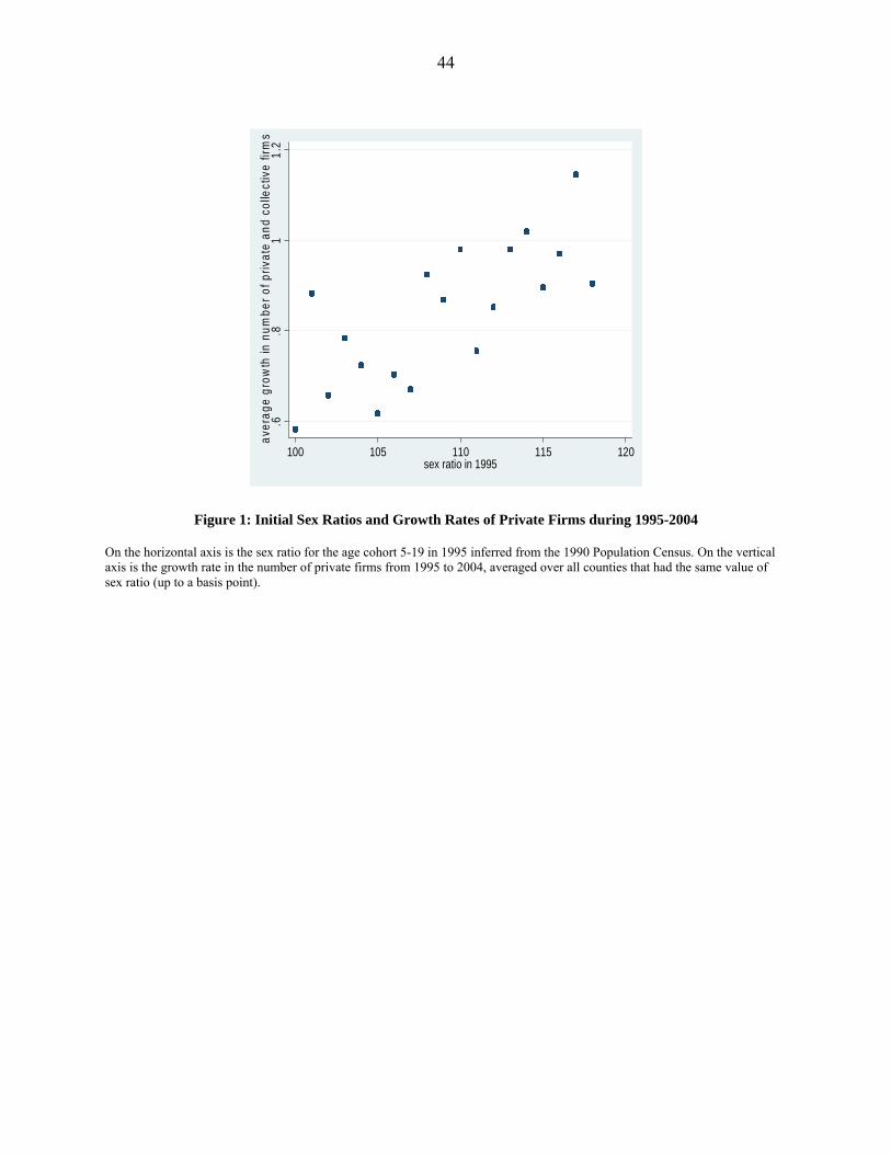
44

 

.6.8

11.

2av

erag

e gr

owth

in n

umbe

r of p

rivat

e an

d co

llect

ive

firm

s

100 105 110 115 120sex ratio in 1995

  

Figure 1: Initial Sex Ratios and Growth Rates of Private Firms during 1995-2004 On the horizontal axis is the sex ratio for the age cohort 5-19 in 1995 inferred from the 1990 Population Census. On the vertical axis is the growth rate in the number of private firms from 1995 to 2004, averaged over all counties that had the same value of sex ratio (up to a basis point).