Several Computational Aeroacoustics solutions for the

ducted diaphragm at low Mach number

Melanie Piellard∗

Delphi Thermal Systems

L-4940 Bascharage, Luxembourg

Christophe Bailly†

Laboratoire de Mecanique des Fluides et d’Acoustique

Ecole Centrale de Lyon & UMR CNRS 5509, 69134 Ecully, France

& Institut Universitaire de France

A hybrid method of aeroacoustic noise computation based on Lighthill’s Acoustic Anal-

ogy is applied to investigate the noise radiated by a low Mach number flow through a ducted

diaphragm. The simulation method is a two-step hybrid approach relying on Lighthill’s

acoustic analogy, assuming the decoupling of noise generation and propagation. The first

step consists of an incompressible Large Eddy Simulation of the turbulent flow field, during

which aerodynamic quantities are recorded. In the second step, a variational formulation

of Lighthill’s Acoustic Analogy using a finite element discretization is solved in the Fourier

space. The sensitive steps consisting in computing and transferring source term data from

the fluid mesh to the acoustic mesh are reviewed. Indeed, as fluid and acoustic meshes

have different constraints due to the different wavelengths to be resolved, interpolation is

required. The method is applied to a three-dimensional ducted diaphragm with low Mach

number flow. Although the configuration is symmetric, this study exhibits a very complex

three-dimensional flow behavior. Four different aerodynamic solutions are compared with

the Direct Noise Computation performed by Gloerfelt & Lafon. Good agreement is found

in terms of mean flow as well as on instantaneous behavior and turbulent intensities. Acous-

tic computations are performed with different mesh refinement and interpolation methods.

Comparison with literature data on similar cases shows the method relevancy.

I. Introduction

In the industrial context, the development of an efficient hybrid noise computation method has to bestbalance the computing time and the computational resources required to reach a relevant solution. Inthis work, four aerodynamic solutions obtained with different flow solvers are compared. The completeaeroacoustic process is explained: transfer of aerodynamic data from the CFD mesh to the acoustic mesh,source terms computation, application of filters to damp sources before they reach the acoustic domainboundaries, and resolution of the acoustic propagation problem. In particular, the interpolation of sourceterms onto the acoustic mesh is detailed. Indeed, depending on the interpolation method chosen, the acousticmesh in source regions may have to be refined to accurately represent source terms. This has a great impacton the computing time and resources necessary for the acoustic finite element simulation. After introducingthe simulation method, its practical implementation is explained, and the interpolation issue is discussed. Themethod is then applied to the case of a ducted diaphragm with a low Mach number flow, with comparisonsbetween different flow solutions, interpolation methods and acoustic processing. Finally, conclusions aredrawn.

∗PhD, melanie.piellard@delphi.com.†Professor, AIAA Senior Member, christophe.bailly@ec-lyon.fr.

1 of 14

American Institute of Aeronautics and Astronautics

16th AIAA/CEAS Aeroacoustics Conference AIAA 2010-3996

Copyright © 2010 by the author(s). Published by the American Institute of Aeronautics and Astronautics, Inc., with permission.

II. Simulation method

The simulation method is a two step hybrid approach relying on Lighthill’s acoustic analogy,1 assumingthe decoupling of noise generation and propagation. The first step consists of an incompressible Large EddySimulation of the turbulent flow field, during which aerodynamic quantities are transiently recorded. Inthe second step, a variational formulation of Lighthill’s Acoustic Analogy discretized by a finite elementdiscretization is solved in the Fourier space, leading to the radiated noise up to the free field thanks to theuse of infinite elements.2

II.A. Theory

The implementation of Lighthill’s acoustic analogy was firstly derived by Oberai et al,3 refer also to ActranUser’s Guide2 and Caro et al4 for instance. The starting point is Lighthill’s equation:

∂2

∂t2(ρ − ρ0) − c2

0

∂2

∂xi∂xi(ρ − ρ0) =

∂2Tij

∂xi∂xj(1)

withTij = ρuiuj + δij

(

(p − p0) − c20(ρ − ρ0)

)

− τij (2)

where ρ is the density and ρ0 its reference value in a medium at rest, c0 is the reference sound velocity, Tij isLighthill’s tensor, ui are the velocity components, p is the pressure and τij is the viscous stress tensor. In ourapplication, with a low Mach number, high Reynolds number flow, the reduced Lighthill’s tensor Tij = ρuiuj

is considered.The variational formulation of Lighthill’s analogy is then obtained after writing the strong variational

statement associated with equation (1), and after integrating by parts along spatial derivatives followingGreen’s theorem. This formulation is actually an equation on the acoustic density fluctuations ρa = ρ − ρ0,which reads:

∫

Ω

(

∂2ρa

∂t2δρ + c2

0

∂ρa

∂xi

∂δρ

∂xi

)

dx = −

∫

Ω

∂Tij

∂xj

∂δρ

∂xidx +

∫

∂Ω=Γ

∂Σij

∂xjni δρ dΓ(x) (3)

where δρ is a test function, Ω designates the computational domain, and Σij is defined as

Σij = ρuiuj + (p − p0)δij − τij . (4)

Two source terms can be distinguished: a volume and a surface contribution. However, when surfaces arefixed, the latest vanishes. Therefore, only the volume source term is considered in this study.

II.B. Practical application

The method consists in coupling a CFD code with a finite element acoustic software where the variationalformulation of Lighthill’s acoustic analogy is implemented. The main steps of a practical computation,provided that an unsteady solution of the flow field has already been obtained, are as follows:

• flow field analysis allows to determine in which flow region(s) acoustic source terms will be considered;an acoustic mesh is built on the whole region of interest for acoustics, with possibly finer elements insource terms regions;

• the time history of the source terms, or of aerodynamic quantities required to compute it, is stored onthe CFD mesh during the CFD computation within the CFD code;

• the source terms, usually computed on the CFD mesh for better accuracy, are interpolated on thecoarser acoustic mesh;

• the unsteady source terms are transformed from time to spectral domain;

• the acoustic computation is performed with Actran/LA,2 taking into account the spectral volumesource terms.

2 of 14

American Institute of Aeronautics and Astronautics

In these five steps, the third one, namely the interpolation from the CFD mesh to the acoustic mesh, is ofprimary importance. Indeed, all the interest of this hybrid aeroacoustic method lies in the decoupling of thenoise generation from its propagation. The decoupling makes it possible to adapt each computational stepwith respect to its efficiency. In particular, the requirements in terms of grid resolution are usually one orderof magnitude more severe in the CFD than in the acoustic computation. This is due to the difference in sizeof acoustic and turbulent wavelengths. Therefore, in order to keep a light and tractable acoustic mesh, anefficient interpolation of source terms from the CFD mesh to the acoustic mesh has to be defined. In thiswork, two types of interpolation are applied. A classical 4th order Lagrange polynomial interpolation on afine acoustic mesh will be compared to a conservative interpolation on a coarse acoustic mesh. Conservativeinterpolation is actually an integration of source terms on the acoustic finite elements. Moreover, it will beshown that the order of finite elements plays an important role when performing integration on a coarsemesh.

III. Case of a ducted diaphragm at low Mach number

III.A. Presentation

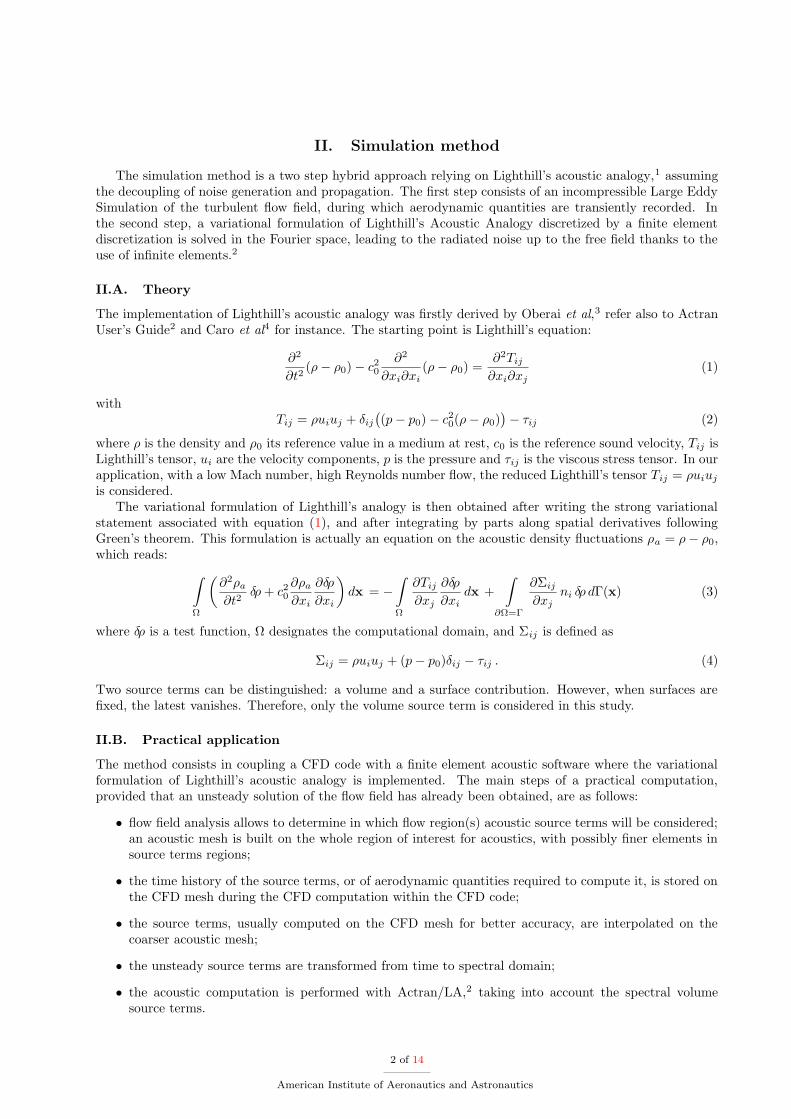
Figure 1. Diaphragm geometry. The x-axis indicates the streamwise flow direction; y- and z-axis respectively indicatethe transverse and spanwise directions.

The case of the ducted diaphragm at low Mach number has been described extensively in Piellard et

al.5,6 It consists of a duct of rectangular cross-section obstructed by a diaphragm of height h, see Figure 1.The aspect ratio defined as w/h, where w is the spanwise duct extension, is equal to 2.86, and the expansionratio defined as D/h, where D is the duct height, is 2.29. In this paper, we study the flow and acousticresults for a very low Mach number flow, with the mean velocity U0 = 6 m/s at the inlet, correspondingto Mach number M = U0/c0 = 0.018. The Reynolds number ReD based on the inlet velocity U0 and ductheight D, and the Reynolds number Reh computed at the diaphragm, based on the maximum mean velocityUb = 20 m/s and obstruction height h, are respectively ReD = 3.3 × 104 and Reh = 4.8 × 104.

This geometry is of particular interest since it represents an internal low velocity flow, for which fewcomputational aeroacoustic studies are available. The present work is based on reference results provided byVan Herpe et al7 who performed experiments in order to get the acoustic power radiated by the diaphragm,and by Gloerfelt & Lafon8 who performed a Direct Noise Computation.

III.B. Four different aerodynamic solutions

As already announced, four different flow solutions are compared in this study. A summary of each calcula-tion’s features is proposed here: mesh, discretization and computing code used.

III.B.1. Incompressible slice simulation: Fluent

The first simulation, later denoted slice incompressible simulation, is performed on a slice of the domainconsisting in 10% of the real width. A structured mesh of 843,000 cells is built, see Figure 2(a), wherethe finest cells in the area of the diaphragm and downstream of the diaphragm are of the order h/70. An

3 of 14

American Institute of Aeronautics and Astronautics

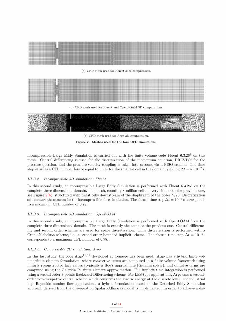
(a) CFD mesh used for Fluent slice computation.

(b) CFD mesh used for Fluent and OpenFOAM 3D computations.

(c) CFD mesh used for Argo 3D computation.

Figure 2. Meshes used for the four CFD simulations.

incompressible Large Eddy Simulation is carried out with the finite volume code Fluent 6.3.269 on thismesh. Central differencing is used for the discretization of the momentum equation, PRESTO! for thepressure question, and the pressure-velocity coupling is taken into account via a PISO scheme. The timestep satisfies a CFL number less or equal to unity for the smallest cell in the domain, yielding ∆t = 5 ·10−7 s.

III.B.2. Incompressible 3D simulation: Fluent

In this second study, an incompressible Large Eddy Simulation is performed with Fluent 6.3.269 on thecomplete three-dimensional domain. The mesh, counting 8 million cells, is very similar to the previous one,see Figure 2(b), structured with finest cells downstream of the diaphragm of the order h/70. Discretizationschemes are the same as for the incompressible slice simulation. The chosen time step ∆t = 10−5 s correspondsto a maximum CFL number of 0.78.

III.B.3. Incompressible 3D simulation: OpenFOAM

In this second study, an incompressible Large Eddy Simulation is performed with OpenFOAM10 on thecomplete three-dimensional domain. The mesh is exactly the same as the previous one. Central differenc-ing and second order schemes are used for space discretization. Time discretization is performed with aCrank-Nicholson scheme, i.e. a second order bounded implicit scheme. The chosen time step ∆t = 10−5 scorresponds to a maximum CFL number of 0.78.

III.B.4. Compressible 3D simulation: Argo

In this last study, the code Argo11,12 developed at Cenaero has been used. Argo has a hybrid finite vol-ume/finite element formulation, where convective terms are computed in a finite volume framework usinglinearly reconstructed face values (typically a Roe’s approximate Riemann solver), and diffusive terms arecomputed using the Galerkin P1 finite element approximation. Full implicit time integration is performedusing a second order 3-points Backward-Differencing scheme. For LES-type applications, Argo uses a second-order non-dissipative central scheme which conserves the kinetic energy at the discrete level. For industrialhigh-Reynolds number flow applications, a hybrid formulation based on the Detached Eddy Simulationapproach derived from the one-equation Spalart-Allmaras model is implemented. In order to achieve a dis-

4 of 14

American Institute of Aeronautics and Astronautics

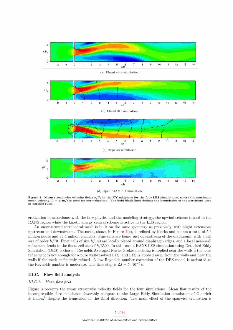
(a) Fluent slice simulation.

(b) Fluent 3D simulation.

(c) Argo 3D simulation.

(d) OpenFOAM 3D simulation.

Figure 3. Mean streamwise velocity fields u/Ub in the XY midplane for the four LES simulations, where the maximummean velocity Ub = 20 m/s is used for normalization. The bold black lines delimit the boundaries of the partitions usedin parallel runs.

cretization in accordance with the flow physics and the modeling strategy, the upwind scheme is used in theRANS region while the kinetic energy central scheme is active in the LES region.

An unstructured tetrahedral mesh is built on the same geometry as previously, with slight extensionsupstream and downstream. The mesh, shown in Figure 2(c), is refined by blocks and counts a total of 5.6million nodes and 33.4 million elements. Fine cells are found just downstream of the diaphragm, with a cellsize of order h/70. Finer cells of size h/140 are locally placed around diaphragm edges, and a local near-wallrefinement leads to the finest cell size of h/3500. In this case, a RANS-LES simulation using Detached EddySimulation (DES) is chosen: Reynolds Averaged Navier-Stokes modeling is applied near the walls if the localrefinement is not enough for a pure wall-resolved LES, and LES is applied away from the walls and near thewalls if the mesh sufficiently refined. A low Reynolds number correction of the DES model is activated asthe Reynolds number is moderate. The time step is ∆t = 5 · 10−5 s.

III.C. Flow field analysis

III.C.1. Mean flow field

Figure 3 presents the mean streamwise velocity fields for the four simulations. Mean flow results of theincompressible slice simulation favorably compare to the Large Eddy Simulation simulation of Gloerfelt& Lafon,8 despite the truncation in the third direction. The main effect of the spanwise truncation is

5 of 14

American Institute of Aeronautics and Astronautics

x/h

y/h

-2 -1 0 1 2 3 4 5 6 7 8 9 10 11 12 13 140

1

2

ArgoOpenFOAMFluent

U/Ub = 1

(a) U/Ub velocity profiles.

x/h

y/h

-2 -1 0 1 2 3 4 5 6 7 8 9 10 11 12 13 140

1

2

ArgoOpenFOAMFluent

V/Ub = 0.5

(b) V/Ub velocity profiles.

x/h

y/h

-2 -1 0 1 2 3 4 5 6 7 8 9 10 11 12 13 140

1

2

ArgoOpenFOAMFluent

W/Ub = 0.1

(c) W/Ub velocity profiles.

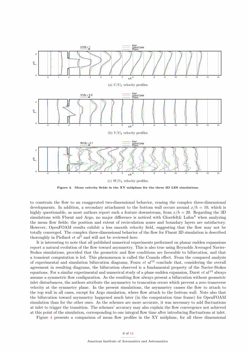
Figure 4. Mean velocity fields in the XY midplane for the three 3D LES simulations.

to constrain the flow to an exaggerated two-dimensional behavior, erasing the complex three-dimensionaldevelopments. In addition, a secondary attachment to the bottom wall occurs around x/h = 10, which ishighly questionable, as most authors report such a feature downstream, from x/h = 20. Regarding the 3Dsimulations with Fluent and Argo, no major difference is noticed with Gloerfelt& Lafon8 when analyzingthe mean flow fields; the position and extent of recirculation zones and boundary layers are satisfactory.However, OpenFOAM results exhibit a less smooth velocity field, suggesting that the flow may not betotally converged. The complex three-dimensional behavior of the flow for Fluent 3D simulation is describedthoroughly in Piellard et al5 and will not be reviewed here.

It is interesting to note that all published numerical experiments performed on planar sudden expansionsreport a natural evolution of the flow toward asymmetry. This is also true using Reynolds Averaged Navier-Stokes simulations, provided that the geometric and flow conditions are favorable to bifurcation, and thata transient computation is led. This phenomenon is called the Coanda effect. From the compared analysisof experimental and simulation bifurcation diagrams, Fearn et al 13 conclude that, considering the overallagreement in resulting diagrams, the bifurcation observed is a fundamental property of the Navier-Stokesequations. For a similar experimental and numerical study of a plane sudden expansion, Durst et al 14 alwaysassume a symmetric flow configuration. As the resulting flow always present a bifurcation without geometricinlet disturbances, the authors attribute the asymmetry to truncation errors which prevent a zero transversevelocity at the symmetry plane. In the present simulations, the asymmetry causes the flow to attach tothe top wall in all cases, except for Argo simulation, where flow attach to the bottom wall. Note also thatthe bifurcation toward asymmetry happened much later (in the computation time frame) for OpenFOAMsimulation than for the other ones. As the schemes are more accurate, it was necessary to add fluctuationsat inlet to trigger the transition. The schemes’ accuracy may also explain the flow convergence not achievedat this point of the simulation, corresponding to one integral flow time after introducing fluctuations at inlet.

Figure 4 presents a comparison of mean flow profiles in the XY midplane, for all three dimensional

6 of 14

American Institute of Aeronautics and Astronautics

x/h

y/h

-2 -1 0 1 2 3 4 5 6 7 8 9 10 11 12 13 140

1

2

ArgoOpenFOAMFluent

u/Ub = 0.2

(a) u′/Ub velocity profiles.

x/h

y/h

-2 -1 0 1 2 3 4 5 6 7 8 9 10 11 12 13 140

1

2

ArgoOpenFOAMFluent

v/Ub = 0.2

(b) v′/Ub velocity profiles.

x/h

y/h

-2 -1 0 1 2 3 4 5 6 7 8 9 10 11 12 13 140

1

2

ArgoOpenFOAMFluent

w/Ub = 0.2

(c) w′/Ub velocity profiles.

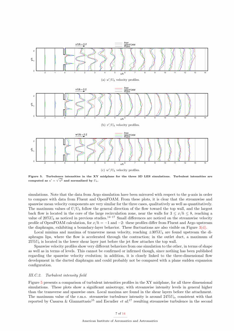
Figure 5. Turbulence intensities in the XY midplane for the three 3D LES simulations. Turbulent intensities are

computed as u′ =√

u2 and normalized by Ub.

simulations. Note that the data from Argo simulation have been mirrored with respect to the y-axis in orderto compare with data from Fluent and OpenFOAM. From these plots, it is clear that the streamwise andspanwise mean velocity components are very similar for the three cases, qualitatively as well as quantitatively.The maximum values of U/Ub follow the general direction of the flow toward the top wall, and the largestback flow is located in the core of the large recirculation zone, near the walls for 3 ≤ x/h ≤ 8, reaching avalue of 20%Ub as noticed in previous studies.14–17 Small differences are noticed on the streamwise velocityprofile of OpenFOAM calculation, for x/h = −1 and −2: these profiles differ from Fluent and Argo upstreamthe diaphragm, exhibiting a boundary-layer behavior. These fluctuations are also visible on Figure 3(d).

Local minima and maxima of transverse mean velocity, reaching ±30%Ub are found upstream the di-aphragm lips, where the flow is accelerated through the contraction; in the outlet duct, a maximum of25%Ub is located in the lower shear layer just before the jet flow attaches the top wall.

Spanwise velocity profiles show very different behaviors from one simulation to the other, in terms of shapeas well as in terms of levels. This cannot be confirmed or infirmed though, since nothing has been publishedregarding the spanwise velocity evolution; in addition, it is closely linked to the three-dimensional flowdevelopment in the ducted diaphragm and could probably not be compared with a plane sudden expansionconfiguration.

III.C.2. Turbulent intensity field

Figure 5 presents a comparison of turbulent intensities profiles in the XY midplane, for all three dimensionalsimulations. These plots show a significant anisotropy, with streamwise intensity levels in general higherthan the transverse and spanwise ones. Local maxima are found in the shear layers before the attachment.The maximum value of the r.m.s. streamwise turbulence intensity is around 24%Ub, consistent with thatreported by Casarsa & Giannattasio15 and Escudier et al;17 resulting streamwise turbulence in the second

7 of 14

American Institute of Aeronautics and Astronautics

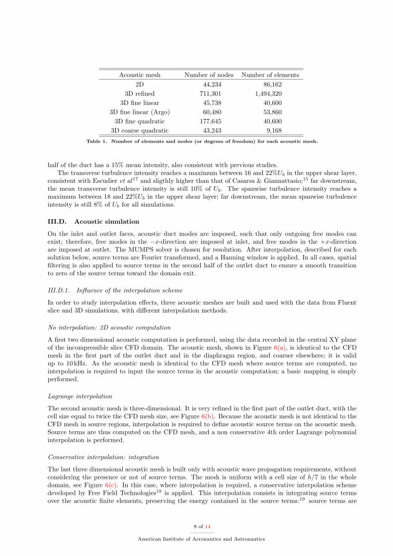
Acoustic mesh Number of nodes Number of elements

2D 44,234 86,162

3D refined 711,301 1,494,320

3D fine linear 45,738 40,600

3D fine linear (Argo) 60,480 53,860

3D fine quadratic 177,645 40,600

3D coarse quadratic 43,243 9,168

Table 1. Number of elements and nodes (or degrees of freedom) for each acoustic mesh.

half of the duct has a 15% mean intensity, also consistent with previous studies.The transverse turbulence intensity reaches a maximum between 16 and 22%Ub in the upper shear layer,

consistent with Escudier et al17 and sligthly higher than that of Casarsa & Giannattasio;15 far downstream,the mean transverse turbulence intensity is still 10% of Ub. The spanwise turbulence intensity reaches amaximum between 18 and 22%Ub in the upper shear layer; far downstream, the mean spanwise turbulenceintensity is still 8% of Ub for all simulations.

III.D. Acoustic simulation

On the inlet and outlet faces, acoustic duct modes are imposed, such that only outgoing free modes canexist; therefore, free modes in the −x-direction are imposed at inlet, and free modes in the +x-directionare imposed at outlet. The MUMPS solver is chosen for resolution. After interpolation, described for eachsolution below, source terms are Fourier transformed, and a Hanning window is applied. In all cases, spatialfiltering is also applied to source terms in the second half of the outlet duct to ensure a smooth transitionto zero of the source terms toward the domain exit.

III.D.1. Influence of the interpolation scheme

In order to study interpolation effects, three acoustic meshes are built and used with the data from Fluentslice and 3D simulations, with different interpolation methods.

No interpolation: 2D acoustic computation

A first two dimensional acoustic computation is performed, using the data recorded in the central XY planeof the incompressible slice CFD domain. The acoustic mesh, shown in Figure 6(a), is identical to the CFDmesh in the first part of the outlet duct and in the diaphragm region, and coarser elsewhere; it is validup to 10 kHz. As the acoustic mesh is identical to the CFD mesh where source terms are computed, nointerpolation is required to input the source terms in the acoustic computation; a basic mapping is simplyperformed.

Lagrange interpolation

The second acoustic mesh is three-dimensional. It is very refined in the first part of the outlet duct, with thecell size equal to twice the CFD mesh size, see Figure 6(b). Because the acoustic mesh is not identical to theCFD mesh in source regions, interpolation is required to define acoustic source terms on the acoustic mesh.Source terms are thus computed on the CFD mesh, and a non conservative 4th order Lagrange polynomialinterpolation is performed.

Conservative interpolation: integration

The last three dimensional acoustic mesh is built only with acoustic wave propagation requirements, withoutconsidering the presence or not of source terms. The mesh is uniform with a cell size of h/7 in the wholedomain, see Figure 6(c). In this case, where interpolation is required, a conservative interpolation schemedeveloped by Free Field Technologies18 is applied. This interpolation consists in integrating source termsover the acoustic finite elements, preserving the energy contained in the source terms:19 source terms are

8 of 14

American Institute of Aeronautics and Astronautics

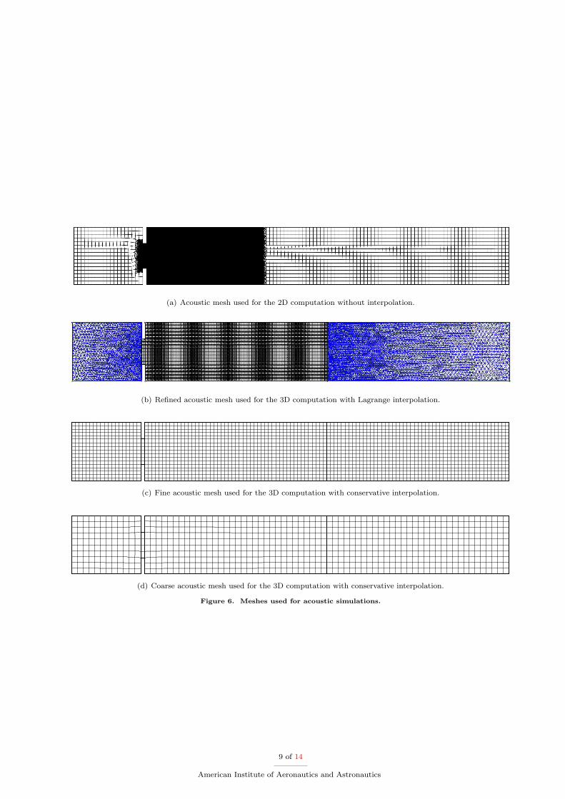
(a) Acoustic mesh used for the 2D computation without interpolation.

(b) Refined acoustic mesh used for the 3D computation with Lagrange interpolation.

X

Y

(c) Fine acoustic mesh used for the 3D computation with conservative interpolation.

X

Y

(d) Coarse acoustic mesh used for the 3D computation with conservative interpolation.

Figure 6. Meshes used for acoustic simulations.

9 of 14

American Institute of Aeronautics and Astronautics

0 500 1000 1500 20000

10

20

30

40

50

60

70

80

90

100

Frequency (Hz)

Lw (d

B/H

z)

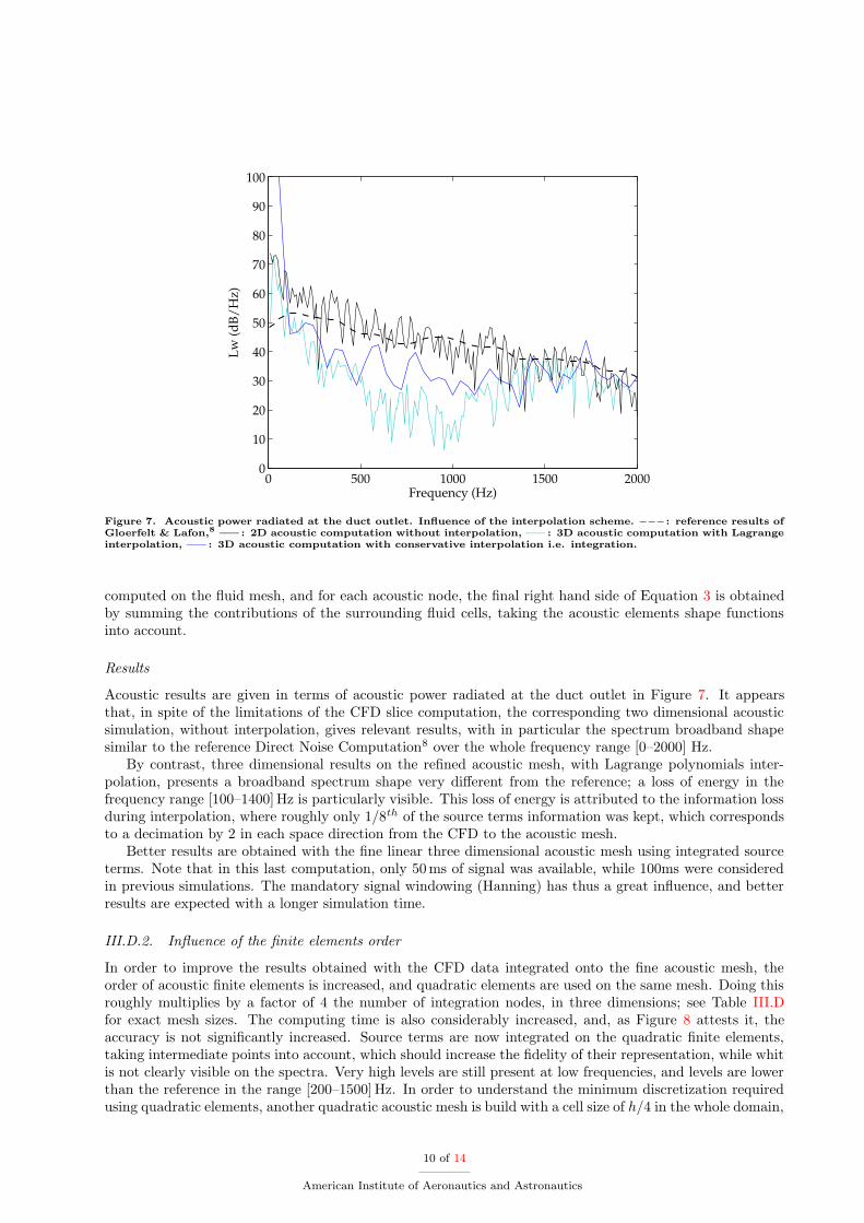
Figure 7. Acoustic power radiated at the duct outlet. Influence of the interpolation scheme. – – – : reference results ofGloerfelt & Lafon,8 —– : 2D acoustic computation without interpolation, —– : 3D acoustic computation with Lagrangeinterpolation, —– : 3D acoustic computation with conservative interpolation i.e. integration.

computed on the fluid mesh, and for each acoustic node, the final right hand side of Equation 3 is obtainedby summing the contributions of the surrounding fluid cells, taking the acoustic elements shape functionsinto account.

Results

Acoustic results are given in terms of acoustic power radiated at the duct outlet in Figure 7. It appearsthat, in spite of the limitations of the CFD slice computation, the corresponding two dimensional acousticsimulation, without interpolation, gives relevant results, with in particular the spectrum broadband shapesimilar to the reference Direct Noise Computation8 over the whole frequency range [0–2000] Hz.

By contrast, three dimensional results on the refined acoustic mesh, with Lagrange polynomials inter-polation, presents a broadband spectrum shape very different from the reference; a loss of energy in thefrequency range [100–1400] Hz is particularly visible. This loss of energy is attributed to the information lossduring interpolation, where roughly only 1/8th of the source terms information was kept, which correspondsto a decimation by 2 in each space direction from the CFD to the acoustic mesh.

Better results are obtained with the fine linear three dimensional acoustic mesh using integrated sourceterms. Note that in this last computation, only 50 ms of signal was available, while 100ms were consideredin previous simulations. The mandatory signal windowing (Hanning) has thus a great influence, and betterresults are expected with a longer simulation time.

III.D.2. Influence of the finite elements order

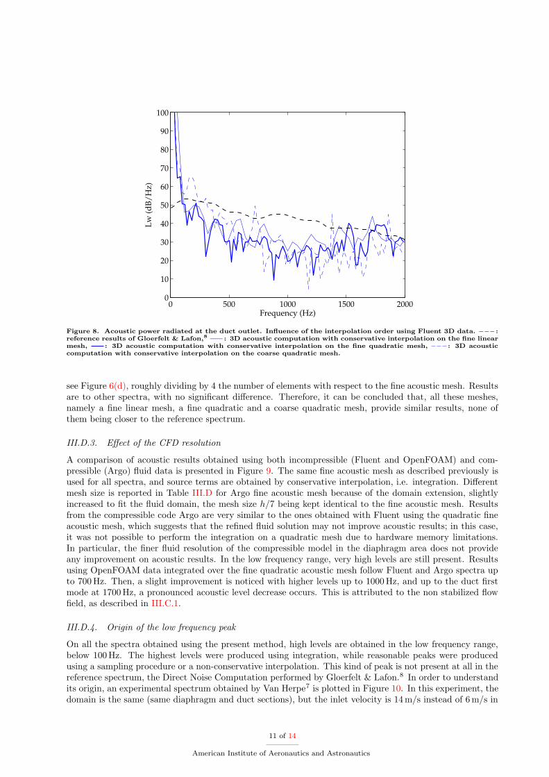
In order to improve the results obtained with the CFD data integrated onto the fine acoustic mesh, theorder of acoustic finite elements is increased, and quadratic elements are used on the same mesh. Doing thisroughly multiplies by a factor of 4 the number of integration nodes, in three dimensions; see Table III.Dfor exact mesh sizes. The computing time is also considerably increased, and, as Figure 8 attests it, theaccuracy is not significantly increased. Source terms are now integrated on the quadratic finite elements,taking intermediate points into account, which should increase the fidelity of their representation, while whitis not clearly visible on the spectra. Very high levels are still present at low frequencies, and levels are lowerthan the reference in the range [200–1500] Hz. In order to understand the minimum discretization requiredusing quadratic elements, another quadratic acoustic mesh is build with a cell size of h/4 in the whole domain,

10 of 14

American Institute of Aeronautics and Astronautics

0 500 1000 1500 20000

10

20

30

40

50

60

70

80

90

100

Frequency (Hz)

Lw (d

B/H

z)

Figure 8. Acoustic power radiated at the duct outlet. Influence of the interpolation order using Fluent 3D data. – – – :reference results of Gloerfelt & Lafon,8 —– : 3D acoustic computation with conservative interpolation on the fine linearmesh, : 3D acoustic computation with conservative interpolation on the fine quadratic mesh, – – – : 3D acousticcomputation with conservative interpolation on the coarse quadratic mesh.

see Figure 6(d), roughly dividing by 4 the number of elements with respect to the fine acoustic mesh. Resultsare to other spectra, with no significant difference. Therefore, it can be concluded that, all these meshes,namely a fine linear mesh, a fine quadratic and a coarse quadratic mesh, provide similar results, none ofthem being closer to the reference spectrum.

III.D.3. Effect of the CFD resolution

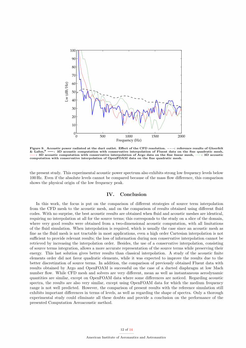
A comparison of acoustic results obtained using both incompressible (Fluent and OpenFOAM) and com-pressible (Argo) fluid data is presented in Figure 9. The same fine acoustic mesh as described previously isused for all spectra, and source terms are obtained by conservative interpolation, i.e. integration. Differentmesh size is reported in Table III.D for Argo fine acoustic mesh because of the domain extension, slightlyincreased to fit the fluid domain, the mesh size h/7 being kept identical to the fine acoustic mesh. Resultsfrom the compressible code Argo are very similar to the ones obtained with Fluent using the quadratic fineacoustic mesh, which suggests that the refined fluid solution may not improve acoustic results; in this case,it was not possible to perform the integration on a quadratic mesh due to hardware memory limitations.In particular, the finer fluid resolution of the compressible model in the diaphragm area does not provideany improvement on acoustic results. In the low frequency range, very high levels are still present. Resultsusing OpenFOAM data integrated over the fine quadratic acoustic mesh follow Fluent and Argo spectra upto 700 Hz. Then, a slight improvement is noticed with higher levels up to 1000 Hz, and up to the duct firstmode at 1700 Hz, a pronounced acoustic level decrease occurs. This is attributed to the non stabilized flowfield, as described in III.C.1.

III.D.4. Origin of the low frequency peak

On all the spectra obtained using the present method, high levels are obtained in the low frequency range,below 100 Hz. The highest levels were produced using integration, while reasonable peaks were producedusing a sampling procedure or a non-conservative interpolation. This kind of peak is not present at all in thereference spectrum, the Direct Noise Computation performed by Gloerfelt & Lafon.8 In order to understandits origin, an experimental spectrum obtained by Van Herpe7 is plotted in Figure 10. In this experiment, thedomain is the same (same diaphragm and duct sections), but the inlet velocity is 14 m/s instead of 6 m/s in

11 of 14

American Institute of Aeronautics and Astronautics

0 500 1000 1500 20000

10

20

30

40

50

60

70

80

90

100

Frequency (Hz)

Lw (d

B/H

z)

Figure 9. Acoustic power radiated at the duct outlet. Effect of the CFD resolution. – – –: reference results of Gloerfelt& Lafon,8 : 3D acoustic computation with conservative interpolation of Fluent data on the fine quadratic mesh,—– : 3D acoustic computation with conservative interpolation of Argo data on the fine linear mesh, —– : 3D acousticcomputation with conservative interpolation of OpenFOAM data on the fine quadratic mesh.

the present study. This experimental acoustic power spectrum also exhibits strong low frequency levels below100 Hz. Even if the absolute levels cannot be compared because of the mass flow difference, this comparisonshows the physical origin of the low frequency peak.

IV. Conclusion

In this work, the focus is put on the comparison of different strategies of source term interpolationfrom the CFD mesh to the acoustic mesh, and on the comparison of results obtained using different fluidcodes. With no surprise, the best acoustic results are obtained when fluid and acoustic meshes are identical,requiring no interpolation at all for the source terms; this corresponds to the study on a slice of the domain,where very good results were obtained from a two-dimensional acoustic computation, with all limitationsof the fluid simulation. When interpolation is required, which is usually the case since an acoustic mesh asfine as the fluid mesh is not tractable in most applications, even a high order Cartesian interpolation is notsufficient to provide relevant results; the loss of information during non conservative interpolation cannot beretrieved by increasing the interpolation order. Besides, the use of a conservative interpolation, consistingof source terms integration, allows a more accurate representation of the source terms while preserving theirenergy. This last solution gives better results than classical interpolation. A study of the acoustic finiteelements order did not favor quadratic elements, while it was expected to improve the results due to thebetter discretization of source terms. In addition, the comparison of previously obtained Fluent data withresults obtained by Argo and OpenFOAM is successful on the case of a ducted diaphragm at low Machnumber flow. While CFD mesh and solvers are very different, mean as well as instantaneous aerodynamicquantities are similar, except on OpenFOAM data where some differences are noticed. Regarding acousticspectra, the results are also very similar, except using OpenFOAM data for which the medium frequencyrange is not well predicted. However, the comparison of present results with the reference simulation stillexhibits important differences in terms of levels, as well as regarding the shape of spectra. Only a thoroughexperimental study could eliminate all these doubts and provide a conclusion on the performance of thepresented Computation Aeroacoustic method.

12 of 14

American Institute of Aeronautics and Astronautics

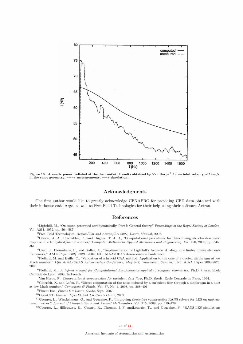
Figure 10. Acoustic power radiated at the duct outlet. Results obtained by Van Herpe7 for an inlet velocity of 14m/s,in the same geometry. – – – : measurements, —– : simulation.

Acknowledgments

The first author would like to greatly acknowledge CENAERO for providing CFD data obtained withtheir in-house code Argo, as well as Free Field Technologies for their help using their software Actran.

References

1Lighthill, M., “On sound generated aerodynamically. Part I: General theory,”Proceedings of the Royal Society of London,Vol. A211, 1952, pp. 564–587.

2Free Field Technologies, Actran/TM and Actran/LA 2007, User’s Manual , 2007.3Oberai, A. A., Roknaldin, F., and Hughes, T. J. R., “Computational procedures for determining structural-acoustic

response due to hydrodynamic sources,” Computer Methods in Applied Mechanics and Engineering, Vol. 190, 2000, pp. 345–361.

4Caro, S., Ploumhans, P., and Gallez, X., “Implementation of Lighthill’s Acoustic Analogy in a finite/infinite elementsframework,” AIAA Paper 2004–2891 , 2004, 10th AIAA/CEAS Aeroacoustics Conference.

5Piellard, M. and Bailly, C., “Validation of a hybrid CAA method. Application to the case of a ducted diaphragm at lowMach number,” 14th AIAA/CEAS Aeroacoustics Conference, May 5–7, Vancouver, Canada, , No. AIAA Paper 2008-2873,2008.

6Piellard, M., A hybrid method for Computational AeroAcoustics applied to confined geometries, Ph.D. thesis, EcoleCentrale de Lyon, 2008, In French.

7Van Herpe, F., Computational aeroacoustics for turbulent duct flow , Ph.D. thesis, Ecole Centrale de Paris, 1994.8Gloerfelt, X. and Lafon, P., “Direct computation of the noise induced by a turbulent flow through a diaphragm in a duct

at low Mach number,” Computers & Fluids, Vol. 37, No. 4, 2008, pp. 388–401.9Fluent Inc., Fluent 6.3 User’s Guide, Sept. 2007.

10OpenCFD Limited, OpenFOAM 1.6 User’s Guide, 2009.11Georges, L., Winckelmans, G., and Geuzaine, P., “Improving shock-free compressible RANS solvers for LES on unstruc-

tured meshes,” Journal of Computational and Applied Mathematics, Vol. 215, 2008, pp. 419–428.12Georges, L., Hillewaert, K., Capart, R., Thomas, J.-F. andLouagie, T., and Geuzaine, P., “RANS-LES simulations

13 of 14

American Institute of Aeronautics and Astronautics

around a complete landing geometry,”Proceedings of the 7th International ERCOFTAC Symposium on Engineering TurbulenceModelling and Measurements, 2008.

13Fearn, R. M., Mullin, T., and Cliffe, K. A., “Nonlinear flow phenomena in a symmetric sudden expansion,” Journal ofFluid Mechanics, Vol. 211, 1990, pp. 595–608.

14Durst, F., Pereira, J. C. F., and Tropea, C., “The plane symmetric sudden-expansion flow at low Reynolds numbers,”Journal of Fluid Mechanics, Vol. 248, 1993, pp. 567–581.

15Casarsa, L. and Giannattasio, P., “Three-dimensional features of the turbulent flow through a planar sudden expansion,”Physics of Fluids, Vol. 20, 2008.

16De Zilwa, S. R. N., Khezzar, L., and Whitelaw, J. H., “Flows through plane sudden-expansions,” International Journalfor Numerical Methods in Fluids, Vol. 32, 2000, pp. 313–329.

17Escudier, M. P., Oliveira, P. J., and Poole, R. J., “Turbulent flow through a plane sudden expansion of modest aspectratio,” Physics of Fluids, Vol. 14, No. 10, 2002, pp. 3641–3654.

18Free Field Technologies, Actran 2009 for Aeroacoustics, User’s Manual , 2009.19Caro, S., Detandt, Y., Manera, J., Toppinga, R., and Mendonca, F., “Validation of a new hybrid CAA strategy and

application to the noise generated by a flap in a simplified HVAC duct,” AIAA Paper 2009–3352 , 2009, 15th AIAA/CEASAeroacoustics Conference.

14 of 14

American Institute of Aeronautics and Astronautics