The direct-hybrid method for computational aeroacoustics on HPC

JARA-HPC Symposium 2016

The direct-hybrid method for computationalaeroacoustics on HPC systems

Michael Schlottke-Lakemper,H. Yu, S. Berger, A. Niemöller, O. CetinA. Lintermann, M. Meinke, W. Schröder

JARA-HPC SimLab Fluids & Solids Engineering andInstitute of AerodynamicsRWTH Aachen University

Aachen, Germany

JHPCS’16, 5th October 2016

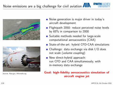
Noise emissions are a big challenge for civil aviation

Sources: Nasa.gov, Wikimedia.org

Noise generation is major driver in today’saircraft developmentFlightpath 2050: reduce perceived noise levelsby 65% in comparison to 2000Suitable methods needed for large-scalecomputational aeroacoustics (CAA)State-of-the-art: hybrid CFD-CAA simulationsChallenge: data exchange via disk I/O doesnot scale (volume coupling)New direct-hybrid approach:run CFD and CAA simultaneously, within-memory data exchange

Goal: high-fidelity aeroacoustics simulation ofaircraft engine jet

2|19 JHPCS’16, 5th October 2016

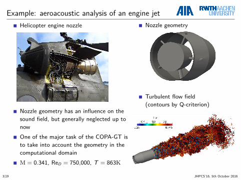
Example: aeroacoustic analysis of an engine jetHelicopter engine nozzle

Nozzle geometry has an influence on thesound field, but generally neglected up tonowOne of the major task of the COPA-GT isto take into account the geometry in thecomputational domainM = 0.341, ReD = 750,000, T = 863K

Nozzle geometry

Turbulent flow field(contours by Q-criterion)


Example: aeroacoustic analysis of an engine jet

10−2

10−1

100

10−6

10−4

10−2

100

St

PS

D(P

a2/S

t)

Model1 fine

Model2 fine

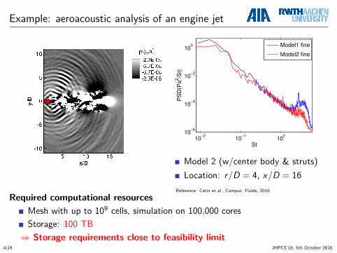
Model 2 (w/center body & struts)Location: r/D = 4, x/D = 16

Reference: Cetin et al., Comput. Fluids, 2016

Required computational resourcesMesh with up to 109 cells, simulation on 100,000 coresStorage: 100 TB⇒ Storage requirements close to feasibility limit


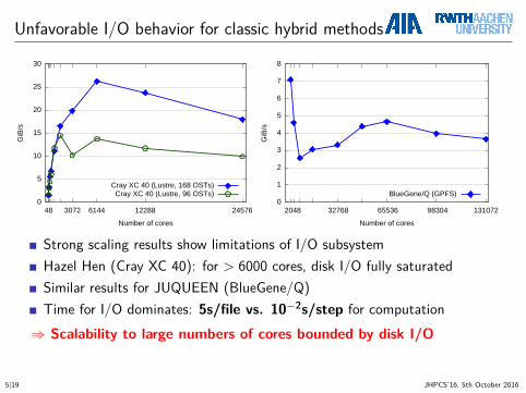
Unfavorable I/O behavior for classic hybrid methods

0

5

10

15

20

25

30

48 3072 6144 12288 24576

GiB

/s

Number of cores

Cray XC 40 (Lustre, 168 OSTs)Cray XC 40 (Lustre, 96 OSTs)

0

1

2

3

4

5

6

7

8

2048 32768 65536 98304 131072

GiB

/s

Number of cores

BlueGene/Q (GPFS)

Strong scaling results show limitations of I/O subsystemHazel Hen (Cray XC 40): for > 6000 cores, disk I/O fully saturatedSimilar results for JUQUEEN (BlueGene/Q)Time for I/O dominates: 5s/file vs. 10−2s/step for computation⇒ Scalability to large numbers of cores bounded by disk I/O


Introducing the direct-hybrid method

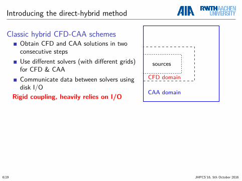
Classic hybrid CFD-CAA schemesObtain CFD and CAA solutions in twoconsecutive stepsUse different solvers (with different grids)for CFD & CAACommunicate data between solvers usingdisk I/O

Rigid coupling, heavily relies on I/O

sources

CFD domain

CAA domain


Introducing the direct-hybrid method

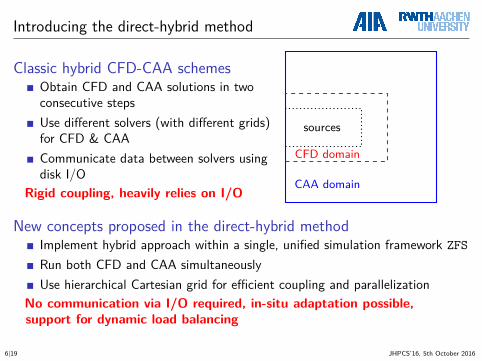
Classic hybrid CFD-CAA schemesObtain CFD and CAA solutions in twoconsecutive stepsUse different solvers (with different grids)for CFD & CAACommunicate data between solvers usingdisk I/O

Rigid coupling, heavily relies on I/O

sources

CFD domain

CAA domain

New concepts proposed in the direct-hybrid methodImplement hybrid approach within a single, unified simulation framework ZFS

Run both CFD and CAA simultaneouslyUse hierarchical Cartesian grid for efficient coupling and parallelization

No communication via I/O required, in-situ adaptation possible,support for dynamic load balancing


Overview

1 The direct-hybrid methodJoint hierarchical Cartesian meshDomain decompositionParallel coupling algorithm

2 Governing equations3 Numerical methods4 Results

Monopole in boundary layerCo-rotating vortex pair

5 Parallel performance6 Summary


Solvers operate on joint hierarchical Cartesian mesh

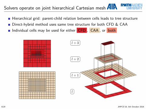
Hierarchical grid: parent-child relation between cells leads to tree structureDirect-hybrid method uses same tree structure for both CFD & CAAIndividual cells may be used for either CFD , CAA , or both

l + 3

l + 2

l + 1

l


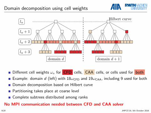
Domain decomposition using cell weights

domain d domain d + 1

Hilbert curvelα

lα + 1

lα + 2

lα + 3

Different cell weights ωx for CFD cells, CAA cells, or cells used for bothExample: domain d (left) with 18ωCFD and 19ωCAA, including 9 used for bothDomain decomposition based on Hilbert curvePartitioning takes place at coarse levelComplete subtrees distributed among ranks

No MPI communication needed between CFD and CAA solver9|19 JHPCS’16, 5th October 2016

Parallel coupling algorithmChallenges for an efficient coupling algorithm

Computational load composition (CFD/CAA cells) varies between domainsSolvers regularly need to exchange data internally(CAA solver may not start before CFD solution available)


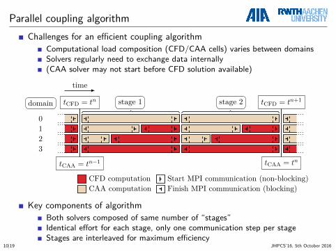
Parallel coupling algorithmChallenges for an efficient coupling algorithm

Computational load composition (CFD/CAA cells) varies between domainsSolvers regularly need to exchange data internally(CAA solver may not start before CFD solution available)

time

tCFD = tn stage 1 stage 2 tCFD = tn+1

tCAA = tn−1 tCAA = tn

CFD computationCAA computation

Start MPI communication (non-blocking)Finish MPI communication (blocking)

domain

0123

Key components of algorithmBoth solvers composed of same number of “stages”Identical effort for each stage, only one communication step per stageStages are interleaved for maximum efficiency


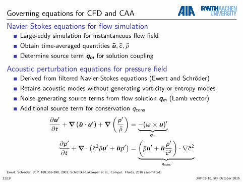
Governing equations for CFD and CAANavier-Stokes equations for flow simulation

Large-eddy simulation for instantaneous flow fieldObtain time-averaged quantities u, c, ρDetermine source term qm for solution coupling

Acoustic perturbation equations for pressure fieldDerived from filtered Navier-Stokes equations (Ewert and Schröder)Retains acoustic modes without generating vorticity or entropy modesNoise-generating source terms from flow solution qm (Lamb vector)Additional source term for conservation qcons

∂u′∂t + ∇ (u · u′) + ∇

(p′ρ

)= −(ω × u)′︸︷︷︸

qm

∂p′∂t + ∇ ·

(c2ρu′ + up′

)=(ρu′ + u p′

c2

)· ∇c2︸︷︷︸

qcons

Ewert, Schröder, JCP, 188:365-398, 2003; Schlottke-Lakemper et al., Comput. Fluids, 2016 (submitted)


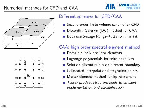
Numerical methods for CFD and CAA

uij

Different schemes for CFD/CAASecond-order finite-volume scheme for CFDDiscontin. Galerkin (DG) method for CAABoth use 5-stage Runge-Kutta for time int.

CAA: high order spectral element methodDomain subdivided into elementsLagrange polynomials for solution/fluxesSolution discontinuous on element boundaryCollocated interpolation/integration pointsMortar element method for hp-refinementTensor product structure leads to efficientimplementation and parallelization


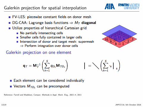
Galerkin projection for spatial interpolation

Reference: Farrell and Maddison, Comput. Methods in Appl. Mech. Eng., 200:1-4, 2011


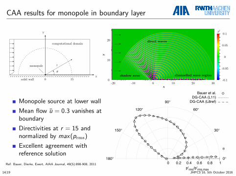
CAA results for monopole in boundary layer

0 15solid wall

rmonopole

computational domain

θ

x

y

Monopole source at lower wallMean flow u = 0.3 vanishes atboundaryDirectivities at r = 15 andnormalized by max(prms)Excellent agreement withreference solution

Ref: Bauer, Dierke, Ewert, AIAA Journal, 49(5):898-908, 2011

-20 -10 0 10 20 30x

0

10

20

y

-0.1

-0.05

0

0.05

0.1p′

shadow zone

direct waves

channelled wave region

0 0.2 0.4 0.6 0.8 10°

30°

60°

90°

120°

150°

180°

θ

p'rms/p'rms,max

Bauer et al.DG-CAA (L11)

DG-CAA (L8ref)


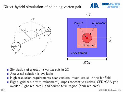
Direct-hybrid simulation of spinning vortex pair

x

y

Γ

Γθ, ω rc

rc

r0

r0

r

(x, y)

Simulation of a rotating vortex pair in 2DAnalytical solution is availableHigh resolution requirements near vortices, much less so in the far fieldRight: grid setup with refinement jumps (concentric circles), CFD/CAA gridoverlap (light red area), and source term region (dark red area)


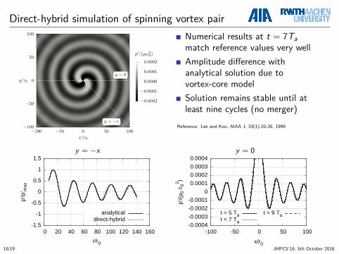
Direct-hybrid simulation of spinning vortex pair

−100 −50 0 50 100x/r0

−100

−50

0

50

100

y/r0

y = 0

y = −x

−0.0002

−0.0001

0.0000

0.0001

0.0002p′/(ρ0c2

0)

Numerical results at t = 7Tamatch reference values very wellAmplitude difference withanalytical solution due tovortex-core modelSolution remains stable until atleast nine cycles (no merger)

Reference: Lee and Koo, AIAA J, 33(1):20-26, 1999

y = −x

-1.5

-1

-0.5

0

0.5

1

1.5

0 20 40 60 80 100 120 140 160

p'/p

' max

r/r0

analyticaldirect-hybrid

y = 0

-0.0004-0.0003-0.0002-0.0001

0 0.0001 0.0002 0.0003 0.0004

-100 -50 0 50 100

p'/(ρ

0 c 0

2 )

x/r0

t = 5 Tat = 7 Ta

t = 9 Ta


Parallel performance: direct-hybrid vs. classic

0

4

8

12

16

20

24

0 500 1000 1500 2000 2500 3000

Spee

dup

Number of cores

ideal speedupdirect-hybrid

classic hybrid

0

0.2

0.4

0.6

0.8

1

1.2

1.4

192 384 768 1536 3072

Wal

l tim

e/st

ep [s

]

Number of cores

direct-hybridI/O (CAA)I/O (LES)

computation (CAA)computation (LES)

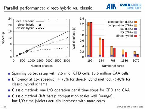
Spinning vortex setup with 7.5 mio. CFD cells, 13.6 million CAA cellsEfficiency at 16x speedup: ≈ 75% for direct-hybrid method, < 40% forclassic hybrid schemeClassic method: one I/O operation per 8 time steps for CFD and CAAClassic method (left bars): computation scales well (orange),but I/O time (violet) actually increases with more cores


Strong scaling of pure CFD/CAA simulations

FV-CFD

0

4

8

12

16

5472 20000 40000 60000 80000 91872

Spee

dup

Number of cores

Ideal speedupFV-CFD

DG-CAA

0 200 400 600 800

1000 1200 1400 1600 1800 2000

48 12288 24576 36864 49152 73728 93600

Spee

dup

Number of cores

Ideal speedup16.8 million cells with 64 DOFs/cell2.1 million cells with 512 DOFs/cell

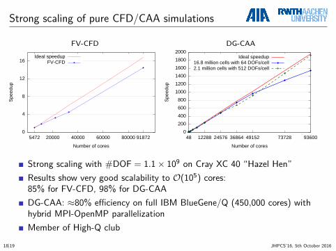
Strong scaling with #DOF = 1.1× 109 on Cray XC 40 “Hazel Hen”Results show very good scalability to O(105) cores:85% for FV-CFD, 98% for DG-CAADG-CAA: ≈80% efficiency on full IBM BlueGene/Q (450,000 cores) withhybrid MPI-OpenMP parallelizationMember of High-Q club


Conclusions

Classic hybrid schemes often do not scale to large numbers of coresA new direct-hybrid approach has been introduced

Unified framework for CFD and CAA simulationsBoth solvers run simultaneously on shared hierarchical Cartesian gridDomain decomposition and coupling algorithm modified for parallel efficiency

Solvers and overall method have been validatedCFD & CAA solvers scale well to large numbers of coresFurther research topics

Large-scale CAA analysis of 3D turbulent jetHybrid CFD-CAA with adaptive mesh refinement and dynamic load balancingCombustion problems with levelset method


Documents

The direct-hybrid method for computational aeroacoustics on HPC