1

Empirical Tests for Market Timing Theory of Capital Structure in Indonesia Stock Exchange

Ignatius Roni Setyawan (ignronis@gmail.com) 62-818-459479(Lecturer from Tarumanagara University (UNTAR), Jakarta, Indonesia)

Budi Frensidy (budi.frensidy@ui.ac.id) 62-816-986734 (Senior Lecturer from Universitas Indonesia (UI), Jakarta, Indonesia)

Paper submitted to the 20th Annual Conference on Pasific Basic Finance, Economis, Accounting and Management

8-9 September 2012, Rutgers University, USA

2

Abstract

This study aims to examine the validity of Market Timing Theory (MTT) from Baker and Wurgler (2002) in the Indonesian context. The essence of MTT is when the market price of a company’s stock is overvalued, the firms will take equity financing and debt financing for undervalued condition. MTT is actually the development of Pecking Order Theory (POT) and Static Trade-Off Theory (STT). The motivations of this study are to test the dispute level of pros and cons of empirical studies about MTT such as Alti (2003) and Wagner (2007) and to check the consistency result of empirical studies of MTT in Indonesia from Dahlan (2004), Kusumawati and Danny (2006), Susilawati (2008), and Saad (2010).

In order to realize the objective, this study will reuse the empirical OLS model from Baker and Wurgler (2002) with some adaptation for Indonesian context. The empirical OLS model from Baker and Wurgler (2002) has a specific uniqueness i.e. the negative relation between leverage and market to book ratio. That negative relationship is controlled by several factors such as earnings after taxes (EAT), total asset, and fixed asset. The other specific uniqueness is the empirical models of MTT are generally applied for IPO-firms.

The result of this study supports the hypothesis of MTT from Baker and Wurgler (2002) in Indonesia Stock Exchange (IDX) with the main finding i.e. market to book ratio has the negative impact to market leverage. While the relevant factor for supporting the hypothesis of MTT is EAT.

Key word : Market Timing Theory, IPO, Market To Book Ratio, Book Leverage, Market Leverage

JEL Classification : G3;G31;G32

3

Empirical Tests for Market Timing Theory of Capital Structure on the Indonesian Stock Exchange

1. INTRODUCTIONManagement does not know the optimal capital structure and neither do the investors.

The issue becomes complex when management must decide the determinant factors of optimal capital structure. The theory of capital structure such as the traditional pecking order theory (POT) and the Static Trade-Off Theory (STT) have not satisfied financial managers in determining the best capital structure policy. Instead they compete with each other in determining the best proxy determinant factors [see Frank and Goyale (2003) and Liu (2005)]. Both theories are quantitative theory-minded. STT has more emphasis on optimal leverage that makes the company safe from financial distress and POT emphasizes the priority in issuing capital. Whereas psychological factors in the capital structure decision according to the behavioralist view like Kant (2003) and Miglo (2010) are also interesting to consider. This is so because the study of Graham and Harvey (2001) has accommodated the psychological approach of capital structure through a survey of CFOs in the USA.

The emergence of Market Timing Theory (MTT) from Baker and Wurgler (2002) is expected to provide "answers"; but it will not be as easy as imagined. MTT proxy in general is the market to book ratio, i.e. in cases of IPO. Many academics as quoted by Huang and Ritter (2005) criticized this proxy because the market to book ratio is generally used a proxy of investment decisions, o find the undervalued or overvalued stocks. Baker and Wurgler (2002) claimed market timing is "the cumulative outcome of past attempts to time the equity market".1 Two assumptions are used namely: 1. Asymmetric information occurs and varies in the capital market such that the rational management is reluctant to make adjustments to the target leverage. 2. Management believes it can do the "timing" of the equity market. The claims of Baker and Wurgler (2002) was successfully derived in empirical models. However, MTT from Baker and Wurgler (2002) raises a lot of pros and cons academically. Pros and cons are not on the second assumption but rather on the first assumption which is the reluctance of of management to do the adjustment towards the target leverage. Based on a survey of Huang and Ritter (2005), scholars who support MTT include Welch (2004); Kayhan and Titman (2005), and Lemmon, et al. (2005). While the cons include the MTT Leary and Robert (2005), and Alti (2003) who was skeptical of the definition of market timing of Baker and Wurgler (2002) and Hovakimian (2005). Pros and Cons of the Market Timing Theory, according to the behavioralist such as Kant (2003) and Miglo (2010), derived from the condition of the company's internal and external factors (capital market situation). Those in support to MTT believe the capital market situation and conditions will affect the investors’ sentiments and the company's internal management in making funding decisions. If the opposite conditions occur, the cons of MTT will prevail [see Vasiliou and Daskalakis (2007)].2

1 Although Kant (2003) and Miglo (2010) said market timing was not a new idea. His view was reinforced by Graham and Harvey (2001) that there was an indication of behavioral management in the equity issuance. Hovakimian et al. (2001) said when the stock price rises, companies will make equity offerings. Then Tobing (2008) and Saad (2010) mentioned the problem of adverse selection in the issuance. [for details, see also Frank and Goyale (2003), p.7].

2 Dittmar and Thakor (2007) stated the problems the company faced when issuing equity-related problems were the indications of irrationality among investors and management. Investors and management used more intuition than rationality of the Bayesian theorem (Neoclassical Paradigm) in decision making. According to Vasilou and Daskalis (2007), the concept of market efficiency of Fama and perfect market of MM Theorem became threatened.

4

The leverage of companies publicly traded in the Indonesia Stock Exchange before the financial crisis has increased sharply and tended to fall after the financial crisis. A sharp increase before the crisis can be seen from the easiness to obtain credit and the management of conglomerate took advantage of this condition. But the bank loans were used for their own business group (related lending) which ignores the principle of prudential banking. That is why after the 1998-2002 monetary crisis many commercial banks were forced to "freeze operation" and be "taken-over" by the regulator, Indonesian Banking Restructuring Agency (IBRA). Many conglomerates as bank shareholders tried to restructure the debt and do business efficiency. The companies in the Indonesia Stock Exchange during the financial crisis did not prove easy to implement a targeted optimal capital structure. The POT, STT, and MTT are expected to provide potential solutions for the target leverage (Tobing, 2008). But setting the targeted leverage cannot be done merely on the basis of practical judgment but must also be based on the empirical studies.

On such basis, this study intends to test market timing of capital structure in Indonesia. There are two motivations. First, the debate reconciliation of theoretical study of MTT of Alti (2003) and Hogfeltd & Oborenko (2005) [the opponents of MTT] and the study of Kayhan and Titman (2005) and Wagner (2007) [the pros of MTT]. Second, the research about MTT in BEI (Bursa Efek Indonesia or Indonesia Stock Exchange) has been done only four times. They were conducted by Kusumawati and Danny (2006) which emphasized the effects of long-term persistence of capital structure with MTT method and OCS (optimal capital structure of STT) and Dahlan (2004) which focused on the existence of any indication about the capital structure policy in Indonesia that led to the MTT. In addition, there were also studies by Susilawati (2008) and Saad (2010).

The general objective of this study is to prove that MTT could be applicable in the Indonesia Stock Exchange. Meanwhile the specific objectives3 are: to analyze the influence of market to book ratio on leverage and analyze the influence of other variables (control variables) such as net property, plant and equipment; earnings after tax and total assets on leverage. The urgency of the general objective is to look for evidence of indications of MTT in the BEI, i.e. market value to book ratio will negatively affect leverage. The logic is, when the company experienced high growth (one of its proxies is the market to book ratio), then the company would tend to reduce the use of debt (one of his proxies is leverage). This is because at that time the cost of equity would be less than the cost of debt. This condition usually occurs when a company (which is experiencing the high growth) does an IPO.

While the urgency of the special objectives lies in the discovery of the control variables of MTT. These are the proxies used in the studies done by Baker and Wurgler (2002) and Huang and Ritter (2005) namely net property, plant, and equipment; earnings after tax, and total assets. The role of these variables in influencing the relationship between the market to book ratio and leverage is interesting to study; as the variable market to book ratio will not stand alone as variable. Dahlan (2004), Kusumawati & Danny (2006) and Saad (2010) identified the role of control variables as leverage determinants in addition to the market to book ratio, which proved to be a major determinant of leverage to indicate the validity of the MTT in IDX. Some of these control variables such as EBIT, size, net working capital, and the lagged-leverage have different levels of significance and it is another motive of this study.

3 Some understanding of the variables to proxy MTT will be explained in detail and will be discussed at the operational definitions of variables. Special variables used leverage of book value and market value, like those of Huang and Ritter (2005). The difference between market and book leverage is the market value component of total assets.

5

This study has several contributions. First, it is trying to redesign MTT in terms of assumptions, the core, the explanatory variables, and the research model. Speaking of assumptions, according to this study, there are three important assumptions. First, the targeted leverage is important but when it reaches the optimal leverage is much more important. This will entirely depend on the equity issuance. Another assumption is the company will experience a deficit financing, since it is not enough just to rely on internal financing. Finally a proxy other than the cost of capital such as the characteristics of firms and market conditions are also important [Huang and Ritter (2005) have shown]. MTT, according to the core of this study, says that the company should use the equity when the cost of equity capital is cheap and vice versa when the cost of debt using debt capital is also cheap. But regardless, that companies can use a combination of both when the cost of equity capital is approximately the cost of debt capital. This means the perfect optimality of capital structure can be created. Another thing is the funding decisions are also influenced by the current situation of the company's whether it is an IPO or an SEO. Theoretically, IPO and SEO will affect the company's capital structure. As explanatory variables, the ratio M/B, the intensity of fixed assets of Baker and Wurgler (2002) can all be applied as long as. The variable M/B has a negative impact on leverage. Study of Huang and Ritter (2005) succeeded in adding variables equity risk premium, profitability, firm size, level of sales and net working capital as well as macro variables such as taxes and GDP. The addition of variables extends the findings of Baker and Wurgler (2002). Research models still refer to OLS of Baker and Wurgler (2002), but it could also be a panel data regression as the study of Huang and Ritter (2005).

2. REVIEW OF THEORY2.1. The Development of Capital Structure Theory

As shown in Figure 1, this study introduces the emergence of market timing theory which started from the conventional MM theory of capital structure in the late 50's. Modigliani and Miller (MM) then issued two propositions. The first proposition associated with leverage, arbitrage4, and firm value. While the second was related to leverage, risk5, and cost of capital. Berk and De Marzo (2007) stated that both these propositions led to the assumption that the leverage did not affect firm value, although the main requirement is the perfect market where there are no transaction costs; risks of every business are the same; equitable access to information (symmetric); and rationality and homogeneity of expectations among investors.

After the revision of the MM theory, there were also alternative theories like the pecking order and static trade-off based on the assumption of imperfect markets such as the existence of asymmetric information and the emergence of the financial distress due to the use of debt. In Figure 1, this study suggests the pecking order and the static trade-off has a strong dominance in the 60's s to the 80's. Pecking order (POT) started from the Fortune 500 survey that generated a sequence of funding. That the cost of retained earnings is the least

4 This is based on the allegations that due to the fact that the interest rate for individuals is treated the same as the interest rate for institutions, then the individual investor has extensive access in the capital markets to trade shares of the levered and unlevered firms through homemade leverage. In equilibrium conditions, there will be arbitrage ooportunities when there is a difference between the levered firm value and the unlevered. So high and low debts will be indifferent for the firms.

5 Risk factor is the difference arising from capital cost of levered and unlevered firms multiplied by the amount of debt. The larger the debt the higher the cost of equity capital. It is due to the fact that the tax-shield effect of the debt will be offset by the increase in equity costs. That situation would make the amount of debt is irrelevant to the firm value.

6

expensive capital, in the view of the respondents, is relevant, because the management does not need high cost for the access of capital.

Whereas the static trade-off (STT) began with the rise of financial experts discussing financial distress as the negative implications of the use of debt. According to STT, debt should be used optimally until the level it will reduce the value of the company. What is interesting is that the best proportion still varies for different industrial sectors; giving rise to "optimal leverage puzzle". In the decade of the 80's and 90's a lot of advanced research in capital structure referred to the STT and POT. Miglo studies (2010) noted two study groups who were pros and cons of the POT. The supporting group to POT were Myers (1984), Baskin (1989), Allen (1993) and Adedeji (1998), whereas those against were Shyam-Sunders and Myers (1999) and Frank and Goyale (2003). Manurung (2004) stated that the different arguments of two groups, pros and cons, were due to differences between the OLS and GLS models which always competed to be the best estimation model and the need for the industrial sector as a determinant of leverage. GLS will be effective when there is a large sample studies (involving the industrial sectors) or cross-country studies such as Mahajan and Tartaroglu’s (2007).

{Figure 1 here}

Since both STT and MTT theories still exist, so this study has the scenario that both the POT and STT inspired the emergence of MTT.6 How can MTT appear? Baker and Wurgler (2002) has stated that the capital structure decisions related to the company's efforts to do the timing of the capital market.

POT and STT proved to be incapable in maximizing the value of the firm and MTT that has a character of "persistence" is expected to be a means of goal achievement financially. The keyword “persistent” becomes MTT superiority in implementation. In the following section, after a detailed discussion of the POT and the STT, the study will discuss it separately. But, as Alti (2003) questioned the nature of such persistence of MTT; this study suspects there are many research gaps that can lead to subsequent studies. Gap research is mainly concerned about the reliability of MTT from Baker and Wurgler (2002) as contemporary theories of capital structure and about the potential problems of MTT because it is dependent on the sample of IPO firms.

2.2. Static Trade-off and Pecking Order TheoriesTable 1 of this study explains the STT and POT using four pillars namely

assumptions, core, variables and research models. Selection of these four pillars is done to more easily discuss a theory by looking at the methodological elements. It can be shown in Table 1 the real differences between STT and POT. POT emphasizes on the hierarchy of funding, while STT underlines heavily the optimality of funding. Although there are striking differences, both focus on the cost of capital (COC). POT focuses on the cheap source of funding, while the STT sticks to the minimum of COC as the main target of capital structure decisions.

{Table 1 here}

6 This study argued that MTT is a "slice" of the POT and the STT. This can be evidenced by MTT recognition that the company should set a target leverage, and provides a strong argument when going to use a source of either debt or equity funds.

7

Some of the explanatory variables in this study were taken from the study of Pangeran (2004). The main model is a logistic regression with an option for financing equity and debt financing options. In line with the study of Pangeran (2004), POT significant explanatory variables are profitability, stock prices, and capital market conditions, all with the positive direction. There are no STT explanatory variables that are significant, that Pangeran (2004) claims POT is more relevant in Indonesia compared to STT. Allegations of this study are related to the period 1991-1996 when the data are a little bullish. Interestingly, Pangeran (2004) adopted the explanatory variables of STT and POT that Bayless and Diltz (1994) used (see underlined italic print in Table 1). That being the case means there is a linkage between STT and POT. Deviation of the target leverage can occur because of the size of the stock offerings and the stock price. The higher the size of the stock offering, the lower the target leverage will be.

2.3. Market Timing Theory (MTT)Similar to the study of Kusumawati and Danny (2006), this study could eventually

define the operation of MTT easily. This is important because Baker and Wurgler (2002) have made little justification of the MTT. Moreover, the groups of researchers who are pros and cons of MTT are just too busy with the persistence problems of MTT in econometrics terms. From Dahlan’s study (2004) and Kusumawati and Danny’s study (2006), MTT showed more important implications of the choice of debt or equity at various time points compared with the search for the optimal leverage ratio. Saad (2010) mentioned two points in time namely during investor sentiment conditions and financial constraints. Our study does not use financial constraint factor on the grounds that the sample is not exposed to the effects of the global financial crisis. Even if it is done, it will be biased because the context of MTT is good reaction from investors.

So, the MTT approach is related to the activity of stock issuance at the IPO or SEO (seasoned equity offering). Baker and Wurgler (2002), Huang and Ritter (2005), and Saad (2010) give four 4 arguments about the effectiveness of MTT (Market Timing Theory) as follows:

1. Companies tend to sell its stake in lieu of debt when market value is high relative to book value and market value of the past is high, and tend to buy back shares when the market value is low.

2. Through the analysis of earning prospects and the expected realization of stock prices around the release of stocks, companies tend to sell its stake at the time investors have high optimism and enthusiasm.

3. If the company experiences financial constraints, then debt funding will be prioritized. The bond contract will discipline the managers.

4. MTT should be done when the company has high growth (growth in the Product Life Cycle) because it would invite a lot of market sentiment.

All the above indicate the importance of overvaluation of a company stock, when it will sell its stake in the market. This is the issue of the MTT version raised by Baker and Wurgler (2002). If the release of shares is more prospective, then market to book ratio (of equity) should have a negative effect on leverage.7 Study of Baker and Wurgler (2002) reinforced the findings of the study by Fama and French (2002) concerning the negative

7 Because this argument is very important for the existence of MTT, the study will spend section 3.4 for the pros and cons of academic research about MTT. Besides, there is also criticism of this study to the definition of persistence used by Kusumawati and Danny (2006) which is too heavy in econometrics.

8

relationship. They even gave recommendations on how the company manages its optimum leverage associated with the market to book ratio (M/B).

Finally this study intends discuss the reciprocal relationship between the M/B ratio with the leverage. Leverage and equity are fundamentally opposite. It can be seen in the right side of a balance sheet. When the debt rises and consequently increase the leverage, the equity portion will fall. What makes the debt proportion rise is the reduction of internal funding or the addition of debt financing.

2.4. Academic Research on Pros and Cons against Market Timing TheoryPros and cons of the MTT range about the persistence of capital structure, whether it

could be long term or not. The results of Baker and Wurgler (2002) successfully demonstrated the persistent effect of equity issuance. If the persistence is still there then the company does not need to rush to do the adjustment of leverage. Huang and Ritter (2005) revealed two groups, one for the pros and the other in the cons of MTT. Among other groups of pros are Welsch (2004), Kayhan and Titman (2005), and Lemmon et al. (2005). They claim that based on the sample of firms that had IPOs, the effect of persistence was still so strong even up to 10-20 years. But with nearly the same samples, Leary and Robert (2005), Alti (2003), and Hovakimian (2005) found the persistence of the effects disappeared in just few years after the IPO. Their study was suspected to have problems with the analysis methods; framework of panel data and a new variable as the trigger factor. Leary and Robert (2005) using GLS which is certainly more robust than OLS from Baker and Wurgler (2002).

Meanwhile, Alti (2003) already incorporated elements of hot and cold IPO markets during the panel data framework, although using the same model (OLS). Last Hovakimian (2005) has included new variables such as size, tangibility and profitability in addition to the M/B and ratios of PPE/Assets and EBITDA/Asset in the study of Baker and Wurgler (2002). With the problems in the persistence definition in the field of econometrics, the study agrees with Huang and Ritter (2005) that an appropriate analysis model is needed. It seems the panel data regression can be an alternative to explain the phenomenon of persistence. Huang and Ritter (2005) has demonstrated the persistence of the effect, although quite weak.

3. RESEARCH METHODOLOGY3.1. Research Procedures

First, researchers will collect data in the Indonesia Stock Exchange of listed companies with active status. Second, researchers will collect data variables to be tested for each company. Third, researchers will conduct OLS regression to test H1 until H4.

3.2. Data Sources and SampleType of data to be retrieved by this study is the companies that went public in 2008

until 2009. Company data is obtained from two sites such as www.idx.co.id and www.finance.yahoo.com and the Indonesian Capital Market Directory (ICMD) 2009 and 2010 and cross-check to the database of OSIRIS from PDBI Indonesian University (UI).

3.3. Sampling TechniquesThe number of companies that went public in the year 2008 up to 2009 is as many as

52 companies including financial institutions. By using a purposive technique, 28 companies are then picked up. Of this number, 14 companies did the IPO in 2008 and 14 companies IPO in 2009. Purposive sampling criteria are:

1. The company is not in the financial sector that is highly-regulated.

9

2. The company was not exposed to the status of delisting during the period 2008-2009, it means the company was not experiencing negative earnings or negative equity due to the global financial crisis of 2008. Thus the sample selected is companies that went public with a high success rate or not affected by the crisis.

3. The company has a complete financial statement information primarily leverage ratio, the number of shares outstanding, and stock prices as of 31 December.8

3.4. Operational Definitions and Relations between VariablesThere are two types of variables, independent variable and dependent variable.

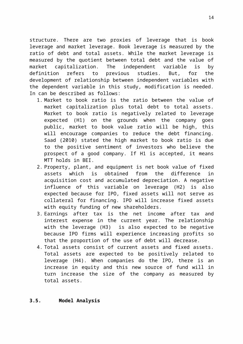
Dependent variable is the level of debt leverage of the company that affects a company's capital structure. There are two proxies of leverage that is book leverage and market leverage. Book leverage is measured by the ratio of debt and total assets. While the market leverage is measured by the quotient between total debt and the value of market capitalization. The independent variable is by definition refers to previous studies. But, for the development of relationship between independent variables with the dependent variable in this study, modification is needed. In can be described as follows:

1. Market to book ratio is the ratio between the value of market capitalization plus total debt to total assets. Market to book ratio is negatively related to leverage expected (H1) on the grounds when the company goes public, market to book value ratio will be high, this will encourage companies to reduce the debt financing. Saad (2010) stated the high market to book ratio is due to the positive sentiment of investors who believe the prospect of a good company. If H1 is accepted, it means MTT holds in BEI.

2. Property, plant, and equipment is net book value of fixed assets which is obtained from the difference in acquisition cost and accumulated depreciation. A negative influence of this variable on leverage (H2) is also expected because for IPO, fixed assets will not serve as collateral for financing. IPO will increase fixed assets with equity funding of new shareholders.

3. Earnings after tax is the net income after tax and interest expense in the current year. The relationship with the leverage (H3) is also expected to be negative because IPO firms will experience increasing profits so that the proportion of the use of debt will decrease.

4. Total assets consist of current assets and fixed assets. Total assets are expected to be positively related to leverage (H4). When companies do the IPO, there is an increase in equity and this new source of fund will in turn increase the size of the company as measured by total assets.

3.5. Model AnalysisThe benchmarked study of this research is Dahlan’s model (2004) which still refers to

the model of Baker and Wurgler (2002). The reason of this benchmarking is the model of Baker and Wurgler (2002) is cited by many research groups such as Susilawati (2008) and Saad (2010). Besides that, the OLS model of Baker and Wurgler (2002) is simpler and more suitable for short-term data like two years or less. The analysis model appears as follows:

ΔBL t = β0 + β1(M/B)t-1 + β2 PPE t-1 + β3 EAT t-1 + β4 TA t-1+ (1)8 Non-financial firms are excluded from the sample. It is based on the consideration that the company's stock

price data is too extreme for the calculation of market to book ratio.

10

ΔML t = β0 + β1(M/B)t-1 + β2 PPE t-1 + β3 EAT t-1 + β4 TA t-1+ (2)

Where:

ΔBL = Book value leverage is expressed as the difference 9

ΔML = Market value of Leverage which is also expressed as the difference

M/B = Market to book ratio

PPE = Net property, plant, and equipment

EAT = Earnings after tax

TA = Total assets

Based on models 1 and 2, in order for H1 until H4 to be accepted, the value of each coefficient β1<0; β2<0; β3<0 and β4>0. Statistically, each coefficient must also have a value of t-count that is significant at minimum level (p-value) 10%. To be used as a predictive model for capital structure decisions in the future, then the models 1 and 2 also have to pass the test of classic assumptions.

4. ANALYSIS RESULT4.1 Descriptive Statistics

Based on Table 2, almost all of the important variables in the model have unique characteristics. ΔBL and ΔML have different characteristics. Market value leverage is generally higher than book value leverage. This is in harmony with the explanation of Kusumawati and Danny (2006) on two factors namely the factors of the deduction from total equity and factors that add market capitalization. Causes of negative values in the book and market leverage are the decreased levels of debt in the sample which implies the acceptance of the MTT hypothesis. Most of the funding is from equity financing that Saad (2010) referred MTT as the Equity Market Timing (EMT).

{Table 2 here}

Independent variables such as M/B, PPE, EAT and the TA have the characteristics of the data namely the standard deviation is larger larger than the mean. This is due to the extreme data of the sample. Extreme data potentially affect the results of the hypothesis testing, but the impact will be small if the number of samples above 30 as a condition to condition i.i.d (independent and identically distributed). To further test the validity of the data prior to analysis, it is necessary to check the correlation between independent variables in Table 3.

{Table 3 here}

9 In the preliminary testing of this study, the result using the absolute values is not satisfying. Then this study decided to use the difference of such values. Setting the difference ΔBL and ΔML as the dependent variables, we express all free variables in model (1) and (2) using the lag (t-1).

11

Based on these tables, it is seen that the variable delta market leverage has a negative close relationship with the market to book ratio. It is significant at the level of 1% as an early indication of the enforceability of MTT. Variables EATt, PPEt-1 also have a negative relationship with the market leverage, although not significantly. This indicates the initial support of the H2 and H3, which means equity financing according to MTT applies when the earnings growth is negative and companies do not need to invest in fixed assets. But these findings are not supported by the fact that the total assets negatively correlated with the market leverage difference, although it is not the case for the book leverage difference.

4.2. Result of Hypothesis TestingIf we see Table 4, the apparent acceptance of H1-H4 will tend to be oriented towards

the market leverage. In models 1 and 2 the coefficient of market to book is even positive. It is rejecting the MTT hypothesis, although variables fixed assets and total assets instead provide results that support H2 and H4. Meanwhile, models 3 and 4 accepted H1-H4. These results support Dahlan's study (2004); Kusumawati and Danny (2006) and Susilawati (2008) and of course Baker and Wurgler (2002). So, for the fourth time MTT proved valid in IDX. But you need to know that the market to book ratio (t-1) would be more fit with market leverage as compared to book leverage. This is the reason the main components of the calculation of market leverage is the market value of total assets. Saad (2010) stated the terms of enforceability from EMT (Equity Market Timing) are a factor of market sentiment to be inherent in the market value of total assets. That means investors in capital markets are more able to control the optimal market leverage than optimal book leverage. When the price of the stock is overpriced (overvalued) then the market value of total assets increased sharply which makes investors reluctant to buy shares of the company. If the project needs funding urgently, then the debt-financing alternatives will be the best choice or the internal equity if the company has retained earnings. This alternative is not consistent with MTT. So the determination of overvaluation and undervaluation will show the validity of EMT.

{Table 4 here}

In econometrics, model 3 clearly says "not feasible" because of the multicollinearity between TA(t-1) and PPE (t-1) with VIF limits more than 10. So this study tested again by dropping the model 4 the PPE(t-1) and TA(t-1). The result is same i.e. H1 and H3 are still acceptable and multicollinearity has disappeared. Actually, to overcome the multicollinearity, the proxy total assets in model 3 can be replaced with the sale. Bu doing so, only models 3 and 4 that can be used as a basis to prove MTT, i.e. when market leverage is used as a proxy for capital structure.

4.3. Result of Hypothesis TestingThere are two models of the Kusumawati and Danny’s study (2006) and Dahlan's

study (2004). Kusumawati and Danny (2006) managed to observe MTT in Indonesia with a data sample of 400 observations from 1991 to 2001 for non-financial companies. The resuts are presented in the form as follows (a black mark for the significant variables):

BL = 0.0197 (M/B)t-1 – 0.0473 (EFWA M/B) t-1 + 0.0048 (PPE/A)t-1 – 0.1274(EBITDA/A)t-1

+ 0.0631 ln (A) t-1 – 0.0019 (S/A) t-1 - 0.4537 (NWCA) t-1 + 0.0698 DUM k

ML= 0.0306 (M/B)t-1 – 0.2946(EFWAM/B)t-1 + 0.108(PPE/A)t-1 – 0.0836 (EBITDA/A)t-1 + 0.0844 ln (A) t-1 – 0.0061 (S/A) t-1 - 0.2291 (NWCA) t-1 + 0.0265 DUM k

12

With this model, Kusumawati and Danny (2006) succeeded in proving the persistence of the effect of MTT even if it is only for short-term (1991-1995) and (1997-2001). While studies of Dahlan (2004) successfully introduced the effects of MTT in the Stock Exchange for non-financial firms (1990-2000). Bleak as Kusumawati and Danny (2006), Dahlan (2004) also used dummy variables of crisis and GLS models. The only important difference is Dahlan (2004) emphasized the variable market leverage not in the magnitude (level) but the difference. The results of the study equation Dahlan (2004) appears as follows (black mark for the significant variables):

ΔLEVt = - 0.533(M/B)t-1–0.098 PPE t-1 – 0.418 EBITt-1 + 9.503 SIZEt-1 – 0.294 ΔLEVt-1

ΔLEVt = -0.51(M/B)t-1–0.11 PPE t-1–0.418 EBITt-1 + 10.414 SIZEt-1–0.283 ΔLEVt-1 – 1.192 DCris t-1

Based on these two studies both Dahlan (2004) and Kusumawati and Danny (2006), then the MTT seems applicable to BEI. But there are challenges that arise in the subsequent research to find the effect of the crisis dummy independent variable in the MTT test. Because crisis dummy is not proven as a determinant of leverage in Dahlan (2004) and Kusumawati and Danny (2006), it is necessary to use an alternative model for robustness check. The importance of this model is to test the effect of persistence of MTT as Baker and Wurgler did (2002) using samples of IPO companies. Alti (2003) highlighted that the companies that went public would be exposed to the phenomenon of long-term market underperformance. That is a decrease in performance (stock price) because more investors are making a sale of shares. As a result, the company cannot conduct an EMT again. The model for this robustness check of GLS model is adopted in model 3.

4.4. Results of the Data Model for Random Effect Model 3 Robustness CheckBased on the simulation model with the GLS random effects in Table 5, all the

independent variables including the M/B(t-1) prove to be significant to MTT. That way the results of MTT testing hypotheses with GLS are better than OLS testing in Table 4. This indicates that testing MTT in Indonesia is more relevant by GLS, due to the variety of the data of leverage, market to book ratio, EAT, PPE, and total assets. The differences between samples of IPO companies cannot well be captured by the OLS. Then some further research in MTT post Baker and Wurgler (2002) recommended the GLS model of fixed effects, random effects, GMM (General Methods of Moment), and also SUR (Seemingly Unrelated Regression). GLS models are capable of lowering the level of autocorrelation which was still frequently encountered in the OLS model, making a low adjusted-R2 as shown in Table 4. With the GLS random effects model in Table 5, all the components of MTT have worked well that H1 to H4 can be accepted. When the individual effects were tested, 78.57% of samples met the conditions for MTT. This finding is one of the GLS superiorities that is capable of sorting out individual samples which are aligned with MTT from those that are not. So, the test results of this study are still valid because it matches the MTT more than 50% that MTT decreases market leverage. This is the condition when market leverage is associated with a market to book ratio; that the market leverage should be low in order to meet the conditions of MTT or EMT.

{Table 5 here}

5. CLOSING NOTES

13

5.1. ConclusionBased on these studies, it appears that using the OLS-model, the MTT hypothesis was

well accepted. This gives wide space for other investigators who want to try the different sample periods and industries. This study also considered the familiarity of panel data regression. The model of this study will be better with a long sample period. Concerning the acceptance of the MTT hypothesis, this study observed the IPO firms used as the sample. There is one unique character of the companies going public in 2008-2009 that the stock prices declined right after the IPO. The phenomenon that occurs is the new investors will take profit; with the assumption that debt levels will rise. Stock price is one component of market to book ratio, so the relationship between market to book and leverage will clearly be negative. This characteristic was exacerbated by the fact that the market to book ratio was also influenced by the EAT which had a negative relationship with leverage. Therefore, the medium-term post-IPO underperformance prevailed. The bottom line profits would tend to decline, even though in the first year after the IPO they tended to rise. The cause of the decline in earnings was management would pay the interest or fund specific projects. It can also be found in the case of pre-emptive rights.

Thus, the general purpose of this research to prove the validity of the MTT Baker and Wurgler (2002) was achieved for the case of IPOs (2008-2009) in the Indonesia Stock Exchange. The results of this study support the findings of Dahlan (2004), Kusumawati and Danny (2006), Susilawati (2008), and Saad (2010). When the analysis for special purposes was done, all determinants of market leverage namely market to book, PPE, EAT, and TA have a significant effect either being tested with OLS or GLS with high R2 values (above 70%). This validates the MTT model of Baker and Wurgler (2002), that all four independent variables as determinants of market leverage can be used in a variety of sample conditions as long as the company is doing an IPO. If the company does not do an IPO, it is necessary to add a relevant determinant variable such as financial constraints as measured by the Kaplan-Zingales Index [see study Saad (2010)]. In the conditions of financial constraint, the market sentiment will be negative, so it is better to delay EMT until the company turns into a positive sentiment.

5.2. Implication5.2.1. Theoretical Implications

One of the biggest problems in testing the MTT is the dependence on the sample of firms that conducted IPO. The investors’ view that IPO is the cheapest source of financing is challenging to be investigated. It is due to the fact that an IPO is usually done during the growth phase of the PLC. This would support the view of EMT. The amount of funds and the stock price in the IPO are set by the underwriter and management. The validity of EMT occurs when a company undergoes IPO process successfully (e.g. Krakatau Steel on November 10, 2010) and the long-term post-IPO performance of companies is also good. If such conditions are met then the assumption of the persistence of the MTT will remain in effect so that Alti’s worries (2003) regarding the inability of long-term test of MTT can be neutralized even though there are many other studies indicating the failure of MTT.

If the company conducts a second stock issue or bond issuance, will EMT or MTT be still relevant? This could be explained that the EMT is dependent on the negative relationship between market leverage and market to book ratio. In the context of debt, then the only way to to do that is to make a positive relationship between market leverage and market to book ratio. It is just a slightly modified MTT concept that the company will add leverage when market to book ratio is still low. The addition of this leverage will not change the context of

14

EMT where optimal market leverage is still relevant. In this case, the management of the company is still following the static trade-off theory. In the context of second share issue, EMT will still be oriented towards a negative relationship between market leverage and market to book ratio, although the power is not as strong as the IPO case. This scenario is when the market to book ratio is no longer at a minimum, the company cannot lower market leverage or increase the equity ratio because it will penetrate the optimum level that will cause the second issue to be less successful. From this argument, the dependence on IPO shares in the context of EMT can be overcome by switching to bonds or a second issue of stocks as long as the optimal leverage at any time can be maintained by management.

5.2.2. Managerial ImplicationsWhen it is learned that the EMT or the MTT can be done not just before the IPO

shares, then the main task of management is to make the process of adjustment at any time towards the optimal market leverage. This adjustment process is very important because it determines the level of market to book ratio that would still have the negative relationship with market leverage. One application of the theory of post-MTT can be used for dynamic capital structure that actually has the initial idea to seek the optimum level of debt arising from the tax reduction benefits and potential costs of bankruptcy by looking at various parameters such as the condition of the company free cash flow, ownership structure, and policy strategies for long-term investment. Dynamic adjustment process in capital structure will certainly strengthen the essence of EMT because it will provide information to management about when they should manage the level of a negative relationship between market leverage and market to book ratio, especially after IPO. If this is an important prerequisite for an IPO, a company can use the essence of this theory that the optimum level of leverage is derived from the initial idea of static trade-off theory (STT).

5.3. LimitationsThere are five limitations of this study. First, our study did not use data of a long

period such as MTT studies in the USA with the period of over 20 years. This is because the study was to focus the uniqueness of the data in 2008-2009. Second, due to the short period, this study could not use panel data regression model (GLS). For “parsimony” reason, this study used the OLS method. Third, the study did not use the data of the financial sector because of its unique behavior as the most highly-regulated industry.

Fourth, the company in the sample should not be exposed to the effects of the global financial crisis. In other words, the company should have no export sales division or have a payable on the imported raw material components. Fifth, several independent variables of leverage to prove the MTT hypothesis were derived from the previous studies by Baker and Wurgler (2002), Dahlan (2004), Danny and Kusumawati (2006), Susilawati (2008) namely market to book ratio and financial ratios. The financial constraint variable of Saad (2010) has not been discussed because it would bias the analysis of IPO company sample.

5.4. SuggestionsThere are two suggestions. They are first, the sample period should be extended to test

the effects of the persistence of the MTT. This is so intensively "attacked" by Alti (2003).

15

Persistency effect is one of the characteristics that has emerged from the MTT. The problem with it is that this effect can only be maintained in the short term, while the capital structure decisions (MTT) is a long-term decision. The use of GMM in Kusumawati and Danny (2006) may be a solution with one note that the data is at least on a quarterly basis. Second, the testing can be extended into several industrial sectors and groups of dummy interaction effects of the global financial crisis in the USA in every industrial sector. The importance of seeing the effects of this crisis is to analyze the truth of the market sentiment from global investors in addressing the effectiveness of the MTT of a company. They should see not only the financial information to estimate the market value to book ratio but also the non-financial information such as the CGPI (Corporate Governance Perception Index) and CSRI (Corporate Social Responsibility Index).

REFERENCESAdedeji, A. (1998), Does the Pecking Order Hypothesis Explain the Dividend Payout Ratios

of Firms in the UK? Journal of Business Finance & Accounting Vol. 25 No.9-10 pp. 1127-1155.

Allen, D.E. (1993), The Pecking Order Hypothesis: Australian Evidence, Applied Financial Economics, Vol. 3 No.2, pp. 101-112.

Alti, A. (2003), How Persistent Is the Impact of Market Timing on Capital Structure, Working Paper from University of Texas Austin, pp. 1-35.

Baker, M. and R. Wurgler (2002), Market Timing and Capital Structure, Journal of Finance 57, pp. 1-32.

Baskin, J. (1989), An Empirical Investigation of the Pecking Order Hypothesis, Financial Management, Vol. 18 No.1, pp. 26-35.

Bayless, M.E. and J.D. Diltz (1994), Securities Offerings and Capital Structure Theory, Journal of Business Finance & Accounting Vol. 21 No.1 pp. 77-91.

Berk, J. and P. De Marzo (2007), Corporate Finance, Pearson International Edition, Chapter 14 dan 15.

Chirinko, R. and A. Singha (2000), Testing Static Trade off Against Pecking Order Models of Capital Structure: A Critical Comment, Journal of Financial Economics Vol. 58, pp. 417 – 425.

Dahlan, I.O. (2004), Market Timing dan Struktur Modal: Studi pada Perusahaan Non Keuangan Tercatat di BEI, Tesis S2 PSIM UI.

Donaldson, G. (1961), Corporate Debt Capacity, Division of Research, Graduate School of Business, Harvard University, Chapter 1.

Elliot, W.B., J.K. Kant and R.S. Warr (2004), Further Evidence on the Financing Deficit: The Impact of Market Timing, Working Paper from Oklahoma State University, pp. 1-32.

Fama, E. F., and K. R. French (2002), Testing Tradeoff and Pecking Order Predictions About Dividends and Debt. Review of Financial Studies Vol. 15, pp. 1-33.

Frank, M.Z. and V.K. Goyale (2003), Capital Structure Decisions, Working Paper from www.ssrn.com,pp. 1-56.

Graham, J.R. and C.R. Harvey (2001), The Theory and Practice of Corporate Finance: Evidence from the Field, Journal of Financial Economics 60,pp. 187-243.

Hogfeldt, P. and A. Oborenko (2005), Does Market Timing or Enhanced Pecking Order Determine Capital Structure? Working Paper from Stockholm School of Economics, pp. 1-48.

Hovakimian, A. (2005), Are Observed Capital Structure Determined by Equity Market Timing? Working Paper from Baruch College, pp. 1-45.

16

Huang, R. and J.R. Ritter (2005), Testing the Market Timing of Capital Structure. Working Paper from University of Florida, pp. 1-44.

Kant, J.K. (2003), Valuation Errors at the Time of Security Issuance dan the Market Timing Theory of Capital Structure, Doctoral Dissertation from Oklahoma State University, pp. 1-123.

Kayhan, A. and S. Titman (2005), Firms’ Histories and Their Capital Structure. NBER Working Paper, pp. 1- 51.

Kusumawati, D. dan F. Danny (2006), Persistensi Struktur Modal Pada Perusahaan Publik Non Keuangan yang Tercatat di BEI: Pendekatan Market Timing dan Teori Struktur Modal Optimal, Jurnal Ekonomi STEI 15 (32), hal. 1-24.

Leary, M.T. and M.R. Robert (2005), Do Firms Rebalance Their Capital Structure?, Journal of Finance, Vol. 60 No. 6, pp. 2575-2619.

Lemmon, M.L., M.R. Robert and J.F. Zender (2005), Back to the Beginning: Persistence and the Cross-Section of Corporate Capital Structure, Working paper from University of Colorado, pp. 1-40.

Liu. L.X. (2005), Do Firms Have Target Leverage Ratios? Evidence from Historical Market to Book and Past Returns, Working Paper from Hongkong University of Science dan Technology, pp. 1-48.

Mahajan, A. and S. Tartaroglu (2007), Equity Market Timing and Capital Structure: International Evidence, Working Paper from Texas A dan M University, pp. 1-32.

Manurung, A.H. (2004), Teori Struktur Modal: Sebuah Survei, Manajemen dan Usahawan Indonesia Vol. 33. No.4, hal.20-25.

Miglo, A. (2010), The Pecking Order, Trade-Off, Signaling and Market Timing Theories of Capital Structure: A Review, Working Paper from University of Bridgeport, pp. 1-26.

Myers, S. C. (1984) The Capital Structure Puzzle. Journal of Finance, 39, 575-592.Pangeran, P. (2004), Pemilihan Antara Penawaran Sekuritas Ekuitas dan Utang: Suatu

Pengujian Empiris terhadap Pecking Order Theory dan Balance Theory, Manajemen dan Usahawan Indonesia Vol.33. No.4, hal. 27-36.

Saad, M.D.P (2010), Pengaruh Sentimen Investor dan Kendala Keuangan Terhadap Equity Market Timing, Disertasi PPIM FE-UI, bab I.

Shyam-Sunder, L., and S. Myers (1999), Testing Static Tradeoff Against Pecking Order Models of Capital Structure. Journal of Financial Economics, 51, 219-244.

Susilawati, C.E. (2008), Implikasi Market Timing Pada Struktur Modal Perusahaan, Makalah Bahan Presentasi 3rd The Doctoral Journey of Management at Crowne Plaza Hotel Jakarta, hal. 1-15.

Tobing, L.R. (2008), Studi Mengenai Perbedaan Struktur Modal Perusahaan Multinasional Dengan Perusahaan Domestik yang Go-Public di Pasar Modal Indonesia: Perspektif Teori Keagenan dan Teori Kontijensi Dalam Mengoptimalkan Struktur Modal Perusahaan, Disertasi Program S3 Ilmu Ekonomi UNDIP, hal. 1-26.

Vasiliou, D. and N. Daskalakis (2007), Behavioral Capital Structure: Is the Neoclassical Paradigm Threatened? Evidence from the Field, Working Paper from Hellenic Open University, pp. 1-31.

Wagner, H.F. (2007), Public Equity Issues and the Scope of Market Timing, Working Paper from London Business School, pp. 1-59.

Welsch, I. (2004), Capital Structure and Stock Return, Journal of Political Economy Vol. 112, pp. 106-131.

Capital Structure Theory

17

Figure 1. Map of Capital Structure Theories Result Analysis from Literature (2010)

Table 1. Comparative between POT and STTDimension POT STT

Market Timing Theory

Pecking Order Theory

Static Trade-Off Theory

Modigliani-Miller Theorem

Gap Theory

1. MTT = POT & STT ?2. MTT = IPO sample?

18

Assumption Preference of internal funding for fear of asymmetric information

Strict dividend policy to "sticky" is usually a low dividend payout ratio

Target leverage Internal and external funding for the

maximization of corporate value

Core Funding by looking at the sequence of the Cost of Capital

Cost of Capital (COC) is cheap generally more dominated by internal financing,

Funding to find the optimal leverage ratio

The use of excessive debt will pose a risk of bankruptcy due to financial distress condition

Explanatory Variable

Profitability & stock price Stock Offering Size

Business Risk Deviation from target leverage

Research Model Baskin (1989) Bayless and Diltz (1994) Allen (1993)

Stiglitz (1969) Bayless and Diltz (1994) Frank and Goyale (2003)

Source: Result Study (2010) from Manurung (2004) and Pangeran (2004)

Table 2. Descriptive Statistics [56 (28X2) observes IPO 2008-2009]

19

Variable Mean Std.Dev Min Max

Δ Book Leverage (BL) -0.0178231 0.1501992 -0.5699379 0.4485325Δ Market Leverage (ML) -0.8324106 2.880701 -16.23754 4.833801Market to Book (M/B) t-1 2.183696 3.0960674 .02289079 17.69324

PPE t-1 0.0982001 0.1580649 0.000103 0.723647EAT t-1 0.0026806 0.013 -0.033934 0.041606

Total Asset (TA) t-1 0.2131082 0.2201024 0.020481 1.021668Source: Result Study (2010) with STATA 9.0

Table 3. Correlation among Independent Variables

Δ BL Δ ML M/B PPE t-1 EAT t-1 TA t-1

Δ BL Pearson Correlation 1 -.192 .101 .144 .312(*) .233

Sig. (2-tailed) . .156 .460 .291 .019 .084N 56 56 56 56 56 56

Δ ML Pearson Correlation -.192 1 -.852(**) -.228 -.243 -.152

Sig. (2-tailed) .156 . .000 .091 .071 .262N 56 56 56 56 56 56

M/B Pearson Correlation .101 -.852(**) 1 .206 .147 .141

Sig. (2-tailed) .460 .000 . .128 .280 .301N 56 56 56 56 56 56

PPE t-1 Pearson Correlation .144 -.228 .206 1 .360(**) .953(**)

Sig. (2-tailed) .291 .091 .128 . .006 .000N 56 56 56 56 56 56

EAT t-1 Pearson Correlation .312(*) -.243 .147 .360(**) 1 .464(**)

Sig. (2-tailed) .019 .071 .280 .006 . .000N 56 56 56 56 56 56

TA t-1 Pearson Correlation .233 -.152 .141 .953(**) .464(**) 1

Sig. (2-tailed) .084 .262 .301 .000 .000 .N 56 56 56 56 56 56

* Correlation is significant at the 0.05 level (2-tailed). ** Correlation is significant at the 0.01 level (2-tailed).

Table 4. Result of Hypothesis Testing [Modification from Dahlan (2004)]

Independent Model 1 Model 2 Model 3 Model 4

20

Variables (dependent variables:

Δ Book Leverage t )

(dependent variables:

Δ Book Leverage t )

(dependent variables: Δ Market

Leverage t )

(dependent variables: Δ Market

Leverage t )Market to Book (t-1)

0.0055903(0.85)1.12

0.0028761(0.45)1.02

-0.7463752(-10.92)***

1.12

-0.7771906(-11.76)***

1.02PPE (t-1) -0.7493058

(-1.7)*12.92

--7.802858(-1.71)*12.92

-

EAT (t-1) 1.782002(1)

1.44

3.398325(2.23)**

1.02

-40.31233(-2.18)**

1.44

-26.98061(-1.72)*

1.02Total Asset (t-1) 0.6115446

(1.86)*14.01

-5.904876(1.74)*14.01

-

Intercept -0.0915507(-2.32)**

-0.0332131(-1.39)

0.4133692(1.01)

0.9370608(3.8)***

F-Hitung 2.31* 2.78* 39.07*** 75.12***Adj-R2 0.0868 0.0609 0.7346 0.7294D-W 2.36 2.188 1.805 1.866

Source: Result Study (2010) with STATA 9.0

Table 5. Result of Hypothesis Testing using Random Effect

Dependent Variable: Δ ML

21

Method: GLS (Variance Components)Date: 01to03to11 Time: 02:08Sample: 1 2Included observations: 2Number of cross-sections used: 28Total panel (balanced) observations: 56

Variable Coefficient Std. Error t-Statistic Prob. C 0.388169 0.442444 0.877331 0.3844

M/B t-1? -0.795363 0.069572 -11.43219 0.0000PPE t-1? -9.757771 4.704509 -2.074132 0.0431EAT t-1? -41.12151 19.12292 -2.150378 0.0363TA t-1? 7.468921 3.557510 2.099480 0.0407

Random Effects

Hypothesis TestingH1 [M/B t-1] ok (MTT)H2[ PPE t-1] okH3[EAT t-1] okH4[ TA t-1] ok

AD [Δ ML] okAK [Δ ML] not okAL [Δ ML] not okeAN [Δ ML] not okeAR [Δ ML] okAS [Δ ML] okBE [Δ ML] okDA [Δ ML] okDH [Δ ML] okDY [Δ ML] okFO [Δ ML] okGO [Δ ML] not okIN [Δ ML] not okIO [Δ ML] okJA [Δ ML] okKA [Δ ML] okKI [Δ ML] okKR [Δ ML] okLA [Δ ML] okLP [Δ ML] not okME [Δ ML] not okPL [Δ ML] okRI [Δ ML] okSU [Δ ML] okSY [Δ ML] not okTP [Δ ML] okTU [Δ ML] okWA [Δ ML] ok

22

_AD--C -0.386628

_AK--C 0.121852_AL--C 0.149593_AN--C 1.788932_AR--C -0.017650_AS--C -0.463395_BE--C -0.007910_DA--C -0.091657_DH--C -0.513837_DY--C -0.002466

_FO--C -0.297117_GO--C 0.023260_IN--C 0.120700_IO--C -0.285217_JA--C -0.106931_KA--C -0.147442_KI--C -0.107705_KR--C -0.111906_LA--C -0.109086_LP--C 1.061136_ME--C 0.294825_PL--C -0.076533_RI--C -0.304147_SU--C -0.102310_SY--C 0.546990_TP--C -0.458469_TU--C -0.188501_WA--C -0.328380

Individual's evidentiary effect in MTT if the coefficient is negative intercept of each company, which means a decrease rather than increase ML. MTT proved valid as many as 22 companies from a total of 28 or approximately 78.57%.

23

GLS Transformed Regression

R-squared 0.815696 Mean dependent var -0.826750

Adjusted R-squared 0.801241 S.D. dependent var 2.882119S.E. of regression 1.284917 Sum squared resid 84.20157Durbin-Watson stat 1.927935

Unweighted Statistics including Random

Effects

R-squared 0.853762 Mean dependent var -0.826750Adjusted R-squared 0.842292 S.D. dependent var 2.882119S.E. of regression 1.144560 Sum squared resid 66.81090Durbin-Watson stat 2.429771

Model Validation:

a. Highly R2

b. Tolerant D-W (2).