Evaluation of Conducting Capital Structure Arbitrage …centerforpbbefr.rutgers.edu/2012PBFEAM/papers/020...Evaluation of Conducting Capital Structure Arbitrage Using the Multi-Period

Evaluation of Conducting Capital Structure Arbitrage Using the

Multi-Period Extended Geske-Johnson Model

By

Hann-Shing Ju, Ren-Raw Chen, Shih-Kuo Yeh and Tung-Hsiao Yang

Hann-Shing Ju is currently a doctoral student in the Department of Finance, National

Chung Hsing University.

Phone: 886-4-22852898.

Fax: 886-4-22856015.

Email: d9821001@ mail.nchu.edu.tw

Ren-Raw Chen is Professor of Finance, Graduate School of Business Administration,

Fordham University.

Phone: 212-636-6471

Fax: 212- 586-0575

Email: [email protected].

Shih-Kuo Yeh is Professor of Finance, National Chung Hsing University.

Phone: 886-4-22852898.

Fax: 886-4-22856015.

Email: [email protected]

Tung-Hsiao Yang is Associate Professor of Finance, National Chung Hsing

University.

Phone: 886-4- 22855571.

Fax: 886-4-22856015.

Email: [email protected]

Evaluation of Conducting Capital Structure Arbitrage Using the

Multi-Period Extended Geske-Johnson Model

Hann-Shing Ju*, Ren-Raw Chen, Shih-Kuo Yeh and Tung-Hsiao Yang

This Version: Feb. 20, 2012

*Corresponding author: Hann-Shing Ju, Doctoral student, Department of Finance, National Chung

Hsing University, Taiwan, Phone: 886-4-22852898, Fax: 886-4-22856015, Email: d9821001@

@mail.nchu.edu.tw. Ren-Raw Chen, Professor of Finance, Graduate School of Business Administration,

Fordham University. Shih-Kuo Yeh, Professor of Finance, National Chung Hsing University, Taiwan.

Tung-Hsiao Yang, Associate Professor of Finance, National Chung Hsing University, Taiwan.

ABSTRACT

This study uses a multi-period structural model developed by Chen and Yeh (2006),

which extends the Geske-Johnson (1987) compound option model to evaluate the

performance of capital structure arbitrage under a multi-period debt structure.

Previous studies exploring capital structure arbitrage have typically employed

single-period structural models, which have very limited empirical scopes. In this

paper, we predict the default situations of a firm using the multi-period

Geske-Johnson model that assumes endogenous default barriers. The Geske-Johnson

model is the only model that accounts for the entire debt structure and imputes the

default barrier to the asset value of the firm. This study also establishes trading

strategies and analyzes the arbitrage performance of 369 North American obligators

from 2004 to 2008. Comparing the performance of capital structure arbitrage between

the Geske-Johnson and CreditGrades models, we find that the extended

Geske-Johnson model is more suitable than the CreditGrades model for exploiting the

mispricing between equity prices and credit default swap spreads.

1

I. Introduction

A trader can theoretically purchase equities and short risky bonds or vice versa to

profit from relative mispricing of these two instruments. This is known as capital

structure arbitrage (or debt-equity trading), and has been the dominant trading activity

in hedge funds specializing in credit security markets. Practitioners believe in existing

cross-market inefficiencies and try to profit from these opportunities. Researchers are

also interested in this issue because the existence of arbitrage profit supports both

cross-market inefficiencies and the usefulness of quantitative credit risk models.

Chatiras and Mukherjee (2004) proposed various ways of conducting capital

structure arbitrage. For example, arbitraging price discrepancy between the

convertible and other forms of company debt is a common form of capital structure

arbitrage (see Calamos (2003)). Another form is to use the pricing discrepancy

between a company’s high yield debt and call options on its stock.

Many arbitragers, however, replace risky bonds with credit default swap

(hereafter CDS) contracts to implement capital structure arbitrage, because CDS

contracts possess more detailed data and have more liquidity than risky bonds. In

addition, many researchers have shown the significant relationship between CDS

spreads and risky bonds spreads.1 This paper uses a structural model to forecast CDS

spreads and conduct different trading strategies based on their forecasted values

relative to the realized counterparts. A significant correlation should theoretically exist

between CDS spreads and equity prices. Thus, institutional investors such as hedge

funds, banks, and insurance companies might apply their trading strategies across

credit and equity markets when the valuation models observe mispricing signals

1 See, for example, Duffie (1999), Lonfstaff et al. (2003) Hull, Predescu, and White (2004),

Houweling and Vorst (2005) and Blanco, Brennan, and Marsh (2005).

2

between a company's CDS spread and equity.

Arbitrage performance, however, can be substantially attributed to model

specification. The nature of capital structure arbitrage is to measure and take

advantage of the difference between model and market spreads. Valuation of CDS

contracts depends on default probability, estimated differently by a variety of

underlying models, which plays an important part in arbitrage performance. Most

models can predict a theoretical spread that significantly correlates with market

spread, but different assumptions regarding the default criteria affect the calculation

of CDS spreads and substantially affect arbitrage performance.

When conducting capital structure arbitrage, arbitragers must employ an

appropriate structural credit risk model to identify arbitrage opportunities. The

structural credit risk models can be traced back to Black and Scholes (1973) and

Merton (1974). The Black-Scholes-Merton option formula can exploit the analogy

between company equity and a call option that underlies the total asset value of the

company with an exercise price equal to the face value of outstanding debt. Chen and

Yeh (2006) indicated that if company value falls below the debt level, equity holders

do not benefit before all debt holders are paid off and the company defaults on the

debt at maturity.

The Merton structural model of valuing equity as a call option is a single-period

model. This model is well developed in relating credit risk to capital structure of a

firm. However, it is only a single period model, which means that a company can

default only at the maturity time of the debt when the debt payment is made. The

bankruptcy triggering mechanism is simple because the model ignores the possibility

of early default. As a result, the model cannot deal with multiple debt structure, which

is considered more realistic.

3

Two approaches extend the Merton structural model: barrier structural models

and compound option models. Barrier structural models assume an exogenous default

barrier, and default is defined as the asset value crossing such a barrier. Black and

Cox (1976) pioneered the definition of default as the first passage time of firm’s value

to a default barrier. However, the compound option models developed by Geske

(1977), and Geske and Johnson (1984) allow a company to have a series of debts.

They employ the compound option pricing technique to characterize default at

different times. The main point is that defaults are a series of contingent events; later

defaults are contingent upon prior no-defaults. Most importantly, the Geske and

Johnson model is the only structural model that endogenously specifies both default

and recovery, while the other structural models assume exogenous barrier and

recovery. Literature investigating whether arbitrage opportunities do exist is scant, even

though debt-equity trading has become popular. Duarte, Longstaff, and Yu (2005)

examined fixed income arbitrage strategies and briefly depicted capital structure

arbitrage. Yu (2006) subsequently focused on capital structure arbitrage and was the

first to conduct a detailed analysis of trading strategies by implementing the

CreditGrades model. Bajlum and Larsen (2008) argued that the opportunities of

capital structure arbitrage could vary with model choice and indicated that model

misspecification should have a significant effect on the gap between the market and

model spreads. Visockis (2011) calculates CDS premiums using two structural

models, namely, the Merton model and the CreditGrades model. The results of the

Merton model show that average monthly capital structure arbitrage returns are

negative. On the other hand, the results of the CreditGrades model show that the

capital structure arbitrage strategy produces significant positive average returns in the

4

investigated period.

Hence, instead of using exogenous default barriers as the CreditGrades model

does, the current research uses a series of endogenous default barriers to calculate

default probabilities across different periods and predicts a theoretical CDS spread

more accurately. This paper adopts the extended Geske-Johnson model by Chen and

Yeh (2006) and uses the similar trading rule developed by Yu (2006) to evaluate

capital structure arbitrage using simulations. Among the related literature, this study is

the first to analyze capital structure arbitrage by implementing the multi-period

structural model with endogenous default barriers.

The CreditGrades model became popular in the credit derivatives market, was

jointly developed by CreditMetrics, JP Morgan, Goldman Sachs, and Deutsche Bank,

and subsequently copy written. Sepp (2006) suggested that this approach supplements

the Merton model (1974) by providing a link to the equity market, particularly to

equity options. The CreditGrades model assumes that firm value follows a pure

diffusion with a stochastic default barrier, introduced to make the model consistent

with high short-term CDS spreads.

Some investment banks have proposed using the CreditGrades model to measure

firm's credit risk. Currie and Morris (2002) and Yu (2006) argued that the

CreditGrades model is the preferred framework among professional arbitrageurs by

testing the historical data. Yu (2006) used the CreditGrades model to implement a

strategy for capital structure arbitrage. The barrier model defines default as the first

time asset value to cross the default barrier. However, the barrier over which the

default is defined is exogenous and arbitrary. This could cause negative equity value,

and an arbitrarily specified barrier could cause incorrect survival probability. Chen

and Yeh (2006) have depicted internal inconsistency of an arbitrarily specified barrier.

5

Yu’s study reveals that the capital structure arbitrageur could suffer substantial losses

at an alarming frequency. The current study suspects that this finding could relate to

model error because the result is based on the CreditGrades model, which assumes an

exogenous barrier and a single period. Hence, its empirical scope is at least limited to

both characteristics.

This paper conducts a capital structure arbitrage using the multi-period

Geske-Johnson model to implement trading analysis. As indicated in Chen and Yeh

(2006), the multi-period Geske-Johnson model is the only model that accounts for the

entire debt structure and imputes the default barrier to the asset value of the firm.

Chen and Yeh (2006) also provided a binomial lattice for implementing the

multi-period Geske-Johnson model instead of conducting expensive high-dimension

normal integrals. This work extends the binominal model using numerical

optimization techniques to assess firm asset value for matching market equity. This

shows that the multi-period Geske-Johnson model can applicably evaluate the credit

default swap spread by n-period risky debts and affect the cumulative profits of

arbitrage when using simulated trading on 369 obligators during 2004 to 2008. To our

knowledge, this is the first paper to apply the multi-period Geske-Johnson model in

predicting the CDS spread and evaluating capital structure arbitrage.

The remainder of the paper is outlined as follows. Section 2 briefly presents the

extended Geske-Johnson model and the CreditGrades model. Section 3 outlines the

trading strategy. Section 4 describes the data. Section 5 conducts an empirical

comparison between the extended Geske-Johnson model and the CreditGrades model.

Section 6 illustrates some case studies. Section 7 presents the general results of the

strategy, and Section 8 concludes all findings.

6

2. Credit Risk Models

The gap between the market and model CDS spread might vary with model

choice because of the substantial difference in model assumptions and methodologies.

The arbitrage signal of relative mispricing is delivered by different models that link

equity and credit derivative markets. However, the arbitrage signal remains stable if

the model can precisely describe CDS spread behavior. This section briefly describes

the CreditGrades model and the extended Geske-Johnson model for pricing CDS

spread as follows. Further details on the two pricing models can be found in Finger

(2002) and Chen and Yeh (2006).

2.1 CreditGrades Model

The CreditGrades model was jointly developed by RiskMetrics, JP Morgan,

Goldman Sachs, and the Deutsche Bank. The model derives from the Merton structure

model for assessing credit risk, including survival probability and credit spread. The

model solves default points with an exogenous default barrier and calculates the CDS

spread with uncertain recovery. Currie and Morris (2002) and Yu (2006) noted that the

CreditGrades model has been used for many years by participants of various credit

derivative markets and has become an industry practice benchmark across numerous

traders.

In the CreditGrades model, the firm asset V is assumed as

t t tdV V dW (1)

whereis the asset volatility and Wt is a standard Brownian motion. The default

barrier is given by

2 / 2ZLD LDe (2)

7

where L is the random recovery rate given default, D is the company’s debt per share,

L

is the mean L,is the standard deviation of ln (L), and Z is a standard normal random

variable. From the perspective of default boundary conditions, the simplest expressions

for asset value and asset volatility are given by:

V S LD (3)

and

s

S

S LD

(4)

where S is equity value, and s is equity volatility. The condition that the firm default

does not occur is

2 2/ 2 / 2

0

Z t WV e LDe (5)

where V0 is initial asset value. The approach solution for survival probability is

expressed as

ln ln

( )2 2

t t

t t

A d A dq t d

A A

(6)

where 2

2 2

0

tA t

V ed

LD

.

is the cumulative normal distribution function. This model can calculate a CDS

spread by linking the survival probability under constant interest rate, given by

1 (0) ( ( ) ( ))

(0, ) (1 )(0) ( ) ( ( ) ( ))

r

rT rT

q e G T Gc T r R

q q T e e G T G

(7)

8

where 2 2/ , and

1/ 2 1/ 2log( ) log( )( ) ( ) ( )z zd d

q T d z T d z TT T

with 21/ 4 2 /z r .

The CreditGrades model is easy to implement in practice and to align with the credit

derivatives market with historical volatility and debt. However, one disadvantage of

the CreditGrades model is its exogenous default barrier, which could cause negative

equity value, and incorrect survival probability. This model is based on the single

period Merton (1974) framework. Consequently, it cannot deal with multi-period debt

structures information, which could be very important in understanding the credit risk

of a firm.

2.2 Extended Geske-Johnson Model

The Geske-Johnson model, initially developed by Geske (1977) and then

corrected by Geske and Johnson (1984), extends the Black-Scholes-Merton model in

the most straightforward manner, in which internal strikes are solved to guarantee

positive equity value. The original Geske-Johnson model has some drawbacks, and is

thus not widely used. The main problems in this model can be attributed to three

reasons: (i) lack of stochastic interest rates, (ii) lack of an efficient implementation

algorithm, and (iii) lack of intuition provided by reduced form and barrier structural

models.

Chen and Yeh (2006) extended the Geske-Johnson model to n periods and

incorporated random interest rates.2 This is necessary because corporate bonds are

2 The formulas provided by Geske (1977) are incorrect and corrected by Geske and Johnson (1984). However, Geske and Johnson only presented formulas for n = 2. Here, we generalize their formulas to an arbitrary n.

9

sensitive to both credit and interest rate risks.3 The current study derives quasi-closed

form solutions similar to those in Geske (1977) and Geske and Johnson (1984) by

providing a simple algorithm for implementing the model. By recognizing only two

state variables (asset price and short interest rate), this article replaces the expensive

high-dimension normal integrals by a fast bi-variate lattice. Lastly, a discrete binomial

framework shows that the Geske-Johnson model carries the same intuition of reduced

form models. Chen and Yeh (2006) extended the Geske-Johnson model to an n period

risky debt. The value of Tn-maturity zero coupon debt can be written as:

1 1 1 11

1 1 1 1 1 1

(0, ) (0, ) [ ( , , ) ( , , )]

(0)[ ( , , ) ( , , )]

n

GJ n i i i n in i n ini

n n n n n n nn

D T P T X k k k k

A k k k k

(8)

where

1 2 1 1 2 2 1 2

1 2

( , , , ) , , , ( , , , )

, ,

i k k ik i k k i ik i

i

k k k N h k h k h k r T r T r T

dr T dr T dr T

for n≥k≥i where is the joint density function of various interest rate levels observed

at different times under the forward measure. Note that kij is a function of r and

j ijh k , for i < j, is defined as

2

2 2 2

0

(0) 1ln (0, )

(0, ) 2( )

(0, )

(0, ) ( , ) 2 ( , )i

i

i ii i

i

T

i A p i Ar A p i

AT

P T Xh X

T

T u T u T du

where A is the diffusion term of asset, p is the diffusion term of interest rate, and

Ar is the correlation between the asset value and the interest rate. The value of the

3 High grade bonds contain more interest rate risk than credit risk.

10

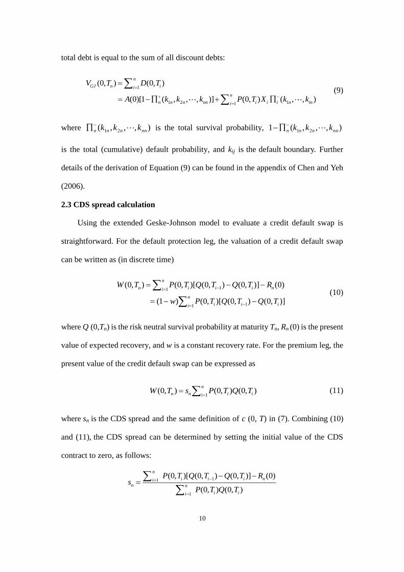
total debt is equal to the sum of all discount debts:

1

1 2 11

(0, ) (0, )

(0)[1 ( , , , )] (0, ) ( , , )

n

GJ n ii

n

n n n nn i i i n ini

V T D T

A k k k P T X k k

(9)

where ),,,( 21 nnnnn kkk is the total survival probability, ),,,(1 21 nnnnn kkk

is the total (cumulative) default probability, and kij is the default boundary. Further

details of the derivation of Equation (9) can be found in the appendix of Chen and Yeh

(2006).

2.3 CDS spread calculation

Using the extended Geske-Johnson model to evaluate a credit default swap is

straightforward. For the default protection leg, the valuation of a credit default swap

can be written as (in discrete time)

11

11

(0, ) (0, )[ (0, ) (0, )] (0)

(1 ) (0, )[ (0, ) (0, )]

n

n i i i ni

n

i i ii

W T P T Q T Q T R

w P T Q T Q T

(10)

where Q (0,Tn) is the risk neutral survival probability at maturity Tn, Rn (0) is the present

value of expected recovery, and w is a constant recovery rate. For the premium leg, the

present value of the credit default swap can be expressed as

1

(0, ) (0, ) (0, )n

n n i iiW T s P T Q T

(11)

where sn is the CDS spread and the same definition of c (0, T) in (7). Combining (10)

and (11), the CDS spread can be determined by setting the initial value of the CDS

contract to zero, as follows:

11

1

(0, )[ (0, ) (0, )] (0)

(0, ) (0, )

n

i i i nin n

i ii

P T Q T Q T Rs

P T Q T

11

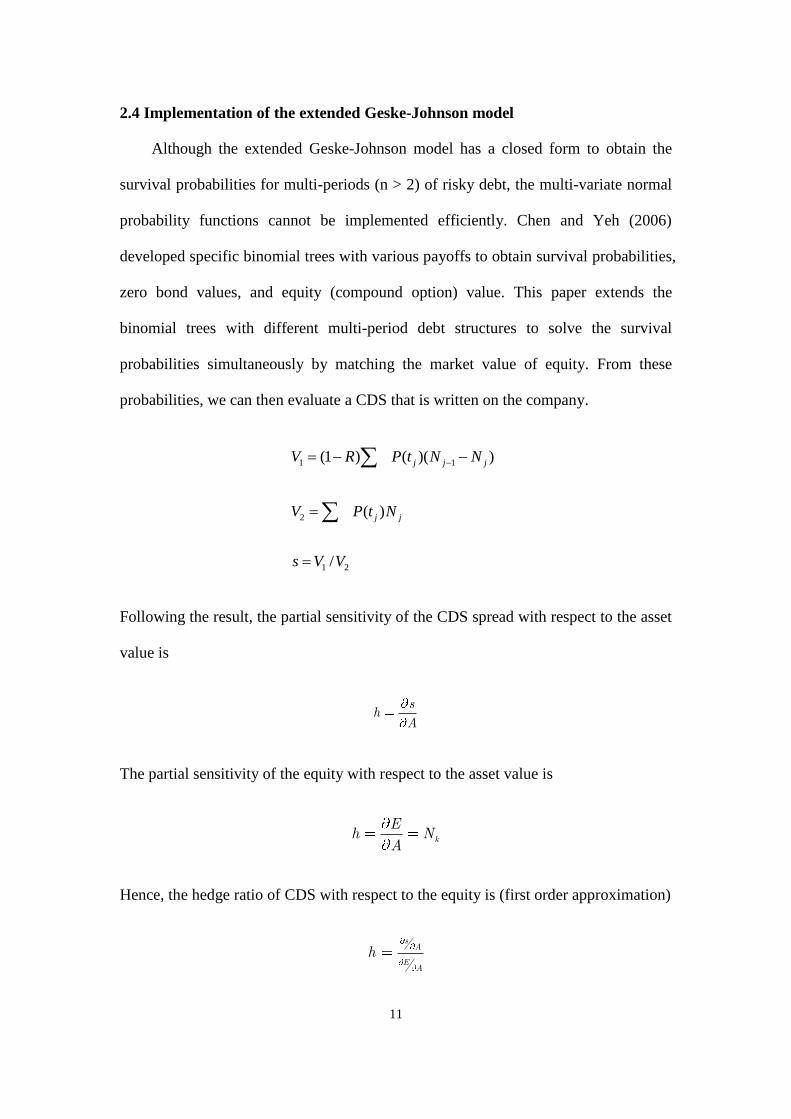
2.4 Implementation of the extended Geske-Johnson model

Although the extended Geske-Johnson model has a closed form to obtain the

survival probabilities for multi-periods (n > 2) of risky debt, the multi-variate normal

probability functions cannot be implemented efficiently. Chen and Yeh (2006)

developed specific binomial trees with various payoffs to obtain survival probabilities,

zero bond values, and equity (compound option) value. This paper extends the

binomial trees with different multi-period debt structures to solve the survival

probabilities simultaneously by matching the market value of equity. From these

probabilities, we can then evaluate a CDS that is written on the company.

1 1

2

1 2

(1 ) ( )( )

( )

/

j j j

j j

V R P t N N

V P t N

s V V

Following the result, the partial sensitivity of the CDS spread with respect to the asset

value is

sh

A

The partial sensitivity of the equity with respect to the asset value is

k

Eh N

A

Hence, the hedge ratio of CDS with respect to the equity is (first order approximation)

sA

EA

h

12

The extended Geske-Johnson model is calibrated each period to the CDS spread

and stock price and hedge ratio are computed. We then compute weekly performance

for some capital structure arbitrage strategies. The main differences between the

CreditGrades model and the extended Geske-Johnson model in capital structure

arbitrage are the theoretical CDS spreads evaluation and the hedge ratios calculation.

Consequently, different models differ in arbitrage strategies and obtain different

arbitrage performances.

3 Trading strategy

A credit default swap (CDS) is a bilateral contract between the buyer and seller

for protection. Defaults are referred to as credit events covered by CDS contracts. The

credit default swap spread is the annual premium amount that the protection buyer

must pay annually or quarterly to the protection seller until the contract ends. If the

reference obligator (company for credit protection) defaults, the protection seller pays

par value of the bond to the protection buyer. CDSs are used to either hedge credit

risk or speculate on changes in CDS spreads for profit.

From the CDS pricing model implementation, the arbitrageur sees an opportunity

by the trading model based on the mispricing between market CDS spread and

theoretical CDS spread. The arbitrageur should either buy CDS and equity or sell both

when mispricing occurs due to the changes in capital structure or volatility. An

arbitrage opportunity exists for co-movements of CDS spreads and stock prices, and the

arbitrageur should obtain a profit from converging spreads or a loss from maintaining

co-movements of CDS spreads and stock prices. Arbitrageurs may see an opportunity

when the credit market is gripped by fear or when the equity market is slow to react if

their views are correct. Hence, many investors develop attractive arbitrage strategies

13

that they keep from other arbitrageurs.

To compare our results with those in Yu (2006), our trading rule follows Yu

(2006) in using the same trigger of arbitrage trading when the gap between actual and

theoretical CDS spreads increases. By defining the trading trigger, the current

market CDS spread ct, and the model CDS spread ˆtc , we initiate a trade if the

following mispricing conditions are satisfied:

ˆ ˆ>(1+ ) or >(1+ )t t t tc c c c (12)

When is satisfied, indicating that the actual market CDS spread is

underpriced, the arbitrageur longs a CDS a notional amount of $1 and buys –shares

of stock as a hedge, whereis a hedge ratio in the trading rule, and vice versa; a

CDS with a notional amount of $1 and –shares of stock is simultaneously shorted if

the condition is satisfied. The condition means that the actual market

CDS spread is overpriced. For hedging CDS contracts, we define the delta hedge in

Equation (13) similarly to Yu (2006):

( , )

( , )= t

t Tt T

E

,

(13)

where ( , )t T

is the value of the CDS contract, Et is the equity price at t, and T is the

maturity date. The delta hedge ratio can be numerically measured by the rate of

change in the CDS contract value relative to the change in equity price. The hedge

ratio determines the number of shares of equity needed to buy or sell for a delta

neutral portfolio. As indicated by Yu (2006), the empirical results are insensitive to the

rebalance of equity position. Therefore, our trading rule adopts a static hedge without

rebalancing between the holding periods. We hold the hedging ratiofixed

ˆ >(1+ )t tc c

ˆ>(1+ )t tc c

14

throughout the holding period. If the spreads converge during the trading period, we

close all the positions.

The purpose of the CDS market is to transfer and hedge credit risk of some

obligators. Trading CDS contracts is quite complicated and requires a sufficiently

huge amount of capital reserve. To simplify the trading process, we assume that the

amount of profit generated has nothing to do with how much capital reserve is

employed. In our trading rule, no trades have to be liquidated early because of capital

limitation. During the holding period or when mispricing convergence occurs, the

value of the equity position is straightforward, and the value of the CDS position is

calculated by varying the CDS spread between c(t, T) and c(0, T).

The profit (or loss) realized from closing trade with equity and CDS is equal to

profit CDS P (14)

where CDS and P correspond to the change in CDS spreads and stock prices

during the holding period or when mispricing convergence occurs. We follow the

suggestion of Yu (2006) to adopt 5% transaction cost for trading CDS and 0%

transaction cost on equities. We assume a $1 notional amount in the CDS without

initial capital limitation for each trade. Because CDS pricing discrepancies are

frequent and persistent, we can compute profit or loss realized by liquidating the CDS

position. Therefore, it is relatively easy to discriminate between the CreditGrades and

the extended Geske-Johnson model to choose a more suitable CDS pricing model for

capital structure arbitrage. Absolute trading return is calculated by each closing trade

and the aggregate profit or loss is generated from the total number of trades.

4. Data

This study collected CDS spreads, equity prices, and debt information of public

15

firms in North America. Data on daily CDS spreads were collected from the category

of Bond Indices and CDS in the DataStream database. We used only five-year CDS

contracts for empirical examination because of liquidity concerns. Firms with a daily

CDS spread and available equity data were included in the sample. However, we

excluded financial firms and their subsidiaries from the sample ensure a consistent

analysis. Debt data were collected from Compustat. Relevant data items included

current liability, total debt, and debt due in the first to fifth years. Debt due

information in the first to fifth year was not entirely available across every firm in the

database. Therefore, we excluded firms with incomplete debt due accounting

information in the first to fifth years. Eventually, we used 369 North American

industrial companies from 2004 to 2008 in the sample.

A multi-period debt structure plays a unique role in the extended Geske-Johnson

model, which assumes that earlier matured debts are more senior than later debts.

Chen and Yeh (2006) assumed that default occurs if the firm fails to meet its cash

obligations at any given time. The cash obligations are exogenously given and can be

regarded as a series of zero coupon bonds issued by the firm. A multi-period debt

structure can be viewed as discrete time barriers, and interpreted as cash obligations at

any point in time. A firm defaults because of its inability to meet short-term cash

obligations rather than meeting total liability.

To construct a complete multi-period debt structure for each firm, this study

measured the first cash obligation by current liability, the second to fifth cash

obligations by debt due in the second to fifth coming year, and the last cash obligation

by total liability subtracted from the sum of the first to fifth cash obligations. We

adopted a six-period debt structure for the entire debt due structure. Table 1 presents

the definition of a six-period debt structure and its item descriptions and mnemonics

16

appearing in the Compustat database. Equity market value is defined as common

shares outstanding at year-end, multiplied by the year-end closing share price. The

risk-free rate is defined as five-year U.S. constant maturity Treasury (CMT) yields

available in the DataStream database.

[Insert Table 1 Here]

5. Model Comparison

This section employs the two models calibrated to total liability and different

debt structures to identify the better model to conduct capital structure arbitrage. In

the CreditGrades model, the input parameters include equity price, equity volatility,

debt-per-share, recovery rate, standard deviation of the default barrier, and risk-free

interest rate. The CreditGrades model is a structural model with an exogenous default

barrier; therefore, the default barrier can be total liability instead of debt per share

(total liability/common shares outstanding). Finger (2002) suggested estimating the

bond-specific recovery rate and the standard deviation of the global recovery rate by

numerically optimizing the pricing model with market CDS spreads. Following

Finger (2002), we assume the bond-specific recovery rate to equal 0.5 and the

standard deviation of the global recovery rate to equal 0.5.

In contrast, calculating CDS spread with a recovery implication in the extended

Geske-Johnson model requires n-period debt setting and firm asset value and asset

volatility. Firm asset value and asset volatility, however, are difficult to measure using

accounting information. This study implements a set of simultaneous equations that

can be solved for asset value and asset volatility by matching equity market value and

its term structure of equity volatility. We adopt a volatility curve in the model to

facilitate the calibration of different CDS spreads. In the original Geske-Johnson

17

model, equity volatility is flat as in the assumption of Black and Scholes (1973).

Unfortunately, under this condition, the calibration of the second bond becomes

impossible. Hence, we extend the model to include a volatility curve, that is,

2 2 2 2(0, ) (0,1) (1,2) ( 1, )v T v v v T T . This flexibility allows us to calibrate the

model to additional market CDS spreads. To examine the spread discrepancy between

two CDS pricing models, we simply maintain a constant risk-free interest rate in a

multi-period setting, although the extended Geske-Johnson model can be

implemented with a term structure interest rate. Table 2 presents the parameter

definitions required for the two pricing models. The parameters shown in the two

models look relatively similar.


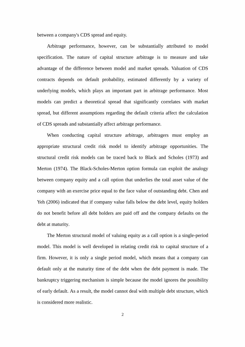
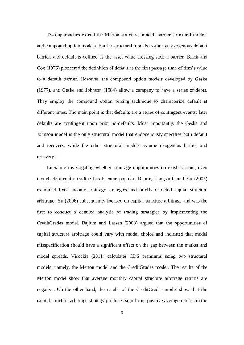
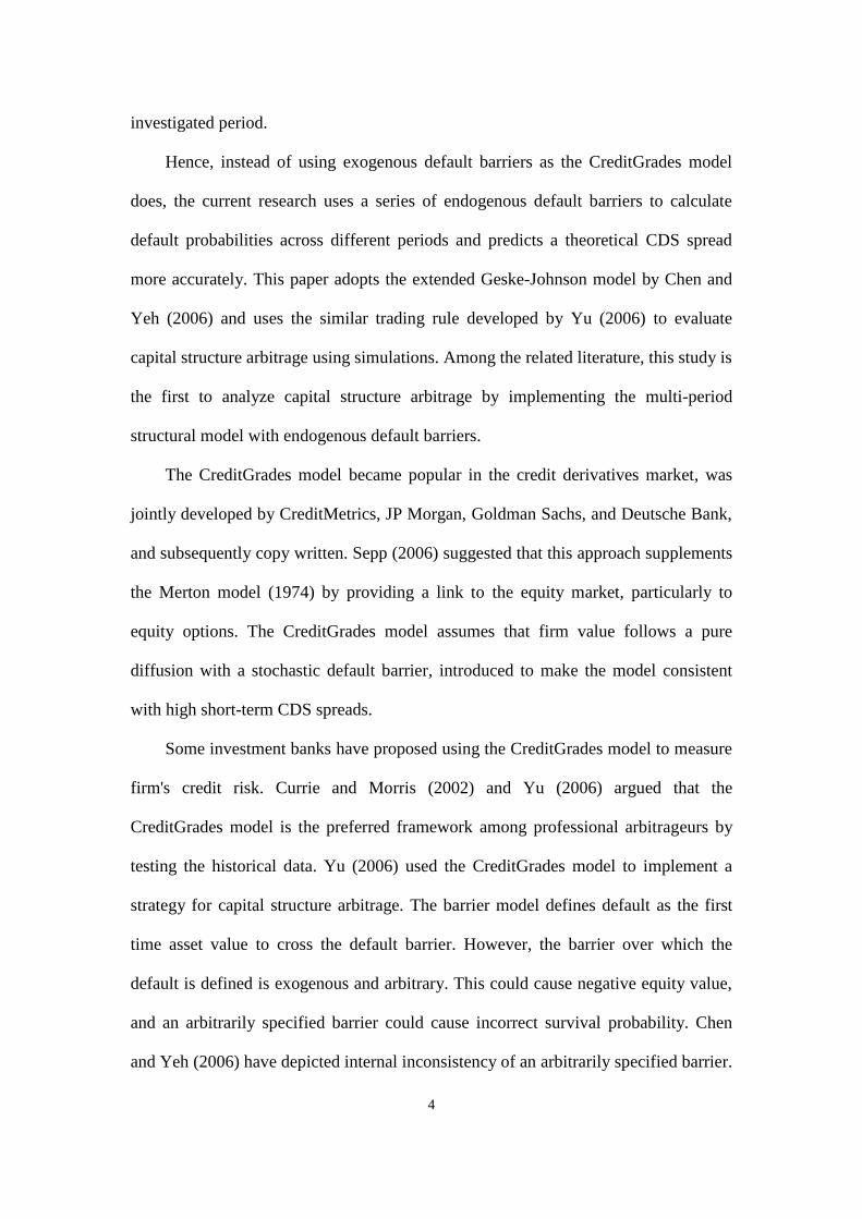
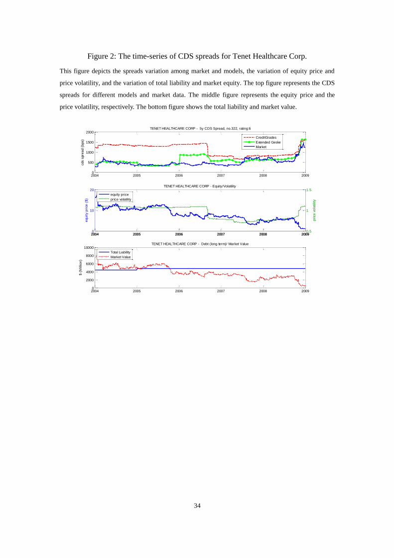
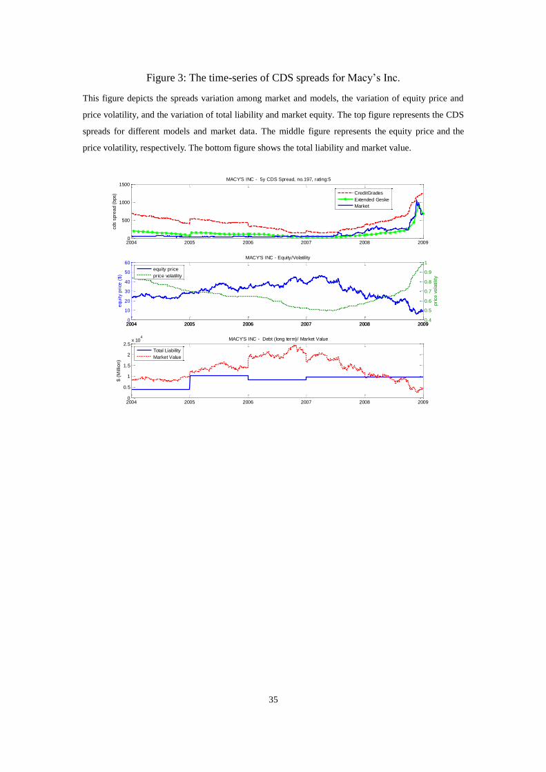
Figures 1 to 3 illustrate the time series of CDS spreads in both models for three

obligators. Each figure depicts the CDS spread discrepancy between market spreads

and those predicted by different models, the trend for equity price and price volatility,

and the trend of total liability and market value. Model spreads appear substantially

less volatile in both models. In normal cases, most of the model spreads calculated in

the two pricing models are roughly in line with market spreads. However, the model

spreads calculated by the extended Geske-Johnson model are considerably closer to

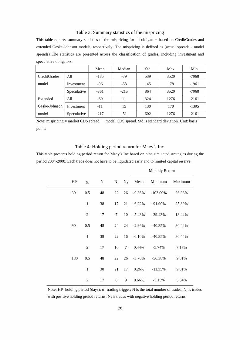
market spreads than the CreditGrades model. Table 3 shows the summary statistics of

mispricing (realized CDS spreads minus forecasted CDS spreads) across the

CreditGrades model and the extended Geske-Johnson model. The extended

Geske-Johnson model performs much better than the CreditGrades model in statistical

comparisons across different categories of all companies, including investment grade

18

and speculative grade obligators. The statistics show that mispricing in investment

grade obligators becomes less dispersed in both models, implying that mispricing

arbitrage returns for investment grade obligators should be better than for speculative

grade obligators.


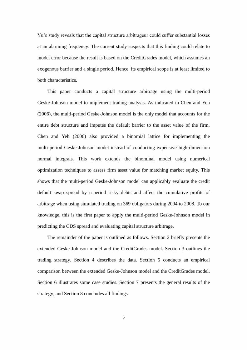
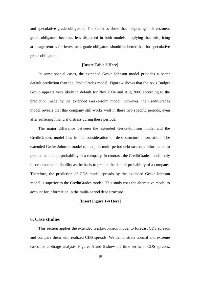
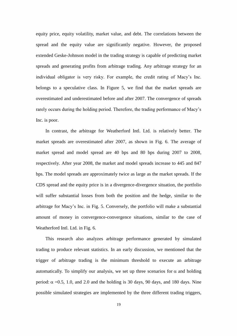
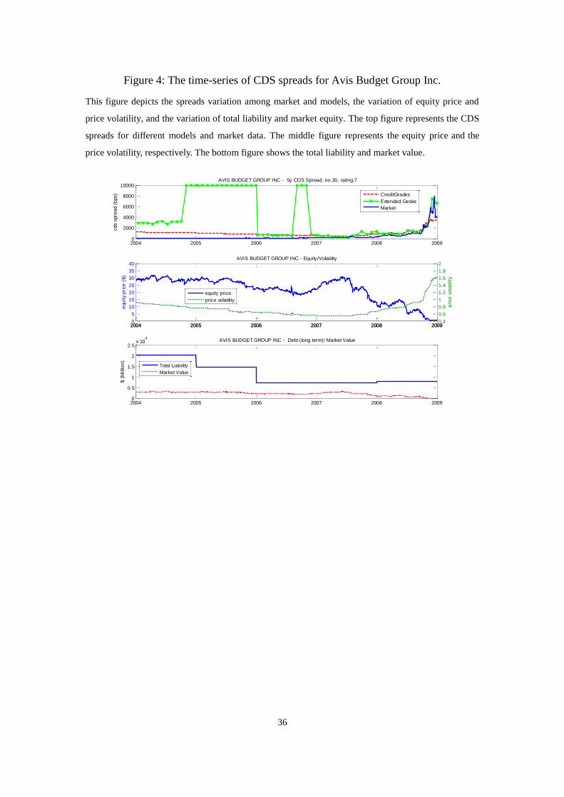
In some special cases, the extended Geske-Johnson model provides a better

default prediction than the CreditGrades model. Figure 4 shows that the Avis Budget

Group appears very likely to default for Nov 2004 and Aug 2006 according to the

prediction made by the extended Geske-John model. However, the CreditGrades

model reveals that this company still works well in these two specific periods, even

after suffering financial distress during these periods.

The major difference between the extended Geske-Johnson model and the

CreditGrades model lies in the consideration of debt structure information. The

extended Geske-Johnson model can exploit multi-period debt structure information to

predict the default probability of a company. In contrast, the CreditGrades model only

incorporates total liability as the basis to predict the default probability of a company.

Therefore, the prediction of CDS model spreads by the extended Geske-Johnson

model is superior to the CreditGrades model. This study uses the alternative model to

account for information in the multi-period debt structure.

[Insert Figure 1-4 Here]

6. Case studies

This section applies the extended Geske-Johnson model to forecast CDS spreads

and compare them with realized CDS spreads. We demonstrate normal and extreme

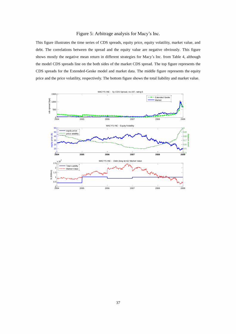
cases for arbitrage analysis. Figures 5 and 6 show the time series of CDS spreads,

19

equity price, equity volatility, market value, and debt. The correlations between the

spread and the equity value are significantly negative. However, the proposed

extended Geske-Johnson model in the trading strategy is capable of predicting market

spreads and generating profits from arbitrage trading. Any arbitrage strategy for an

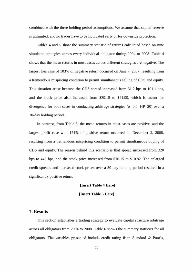
individual obligator is very risky. For example, the credit rating of Macy’s Inc.

belongs to a speculative class. In Figure 5, we find that the market spreads are

overestimated and underestimated before and after 2007. The convergence of spreads

rarely occurs during the holding period. Therefore, the trading performance of Macy’s

Inc. is poor.

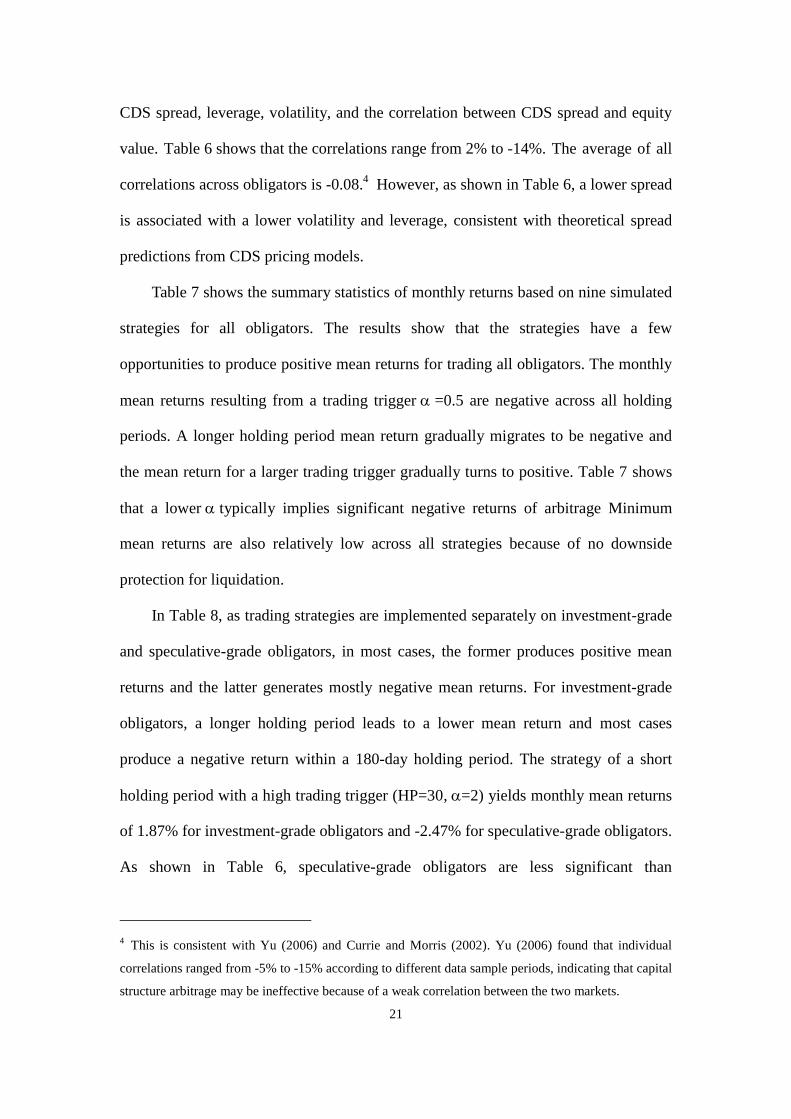
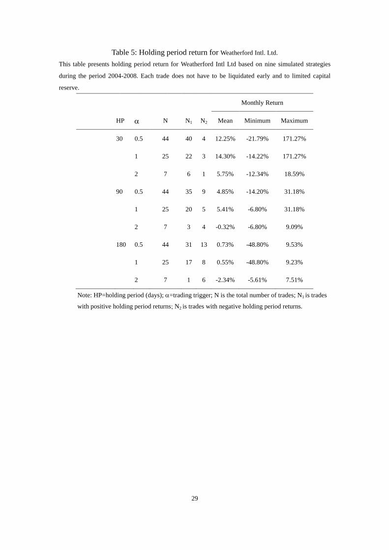
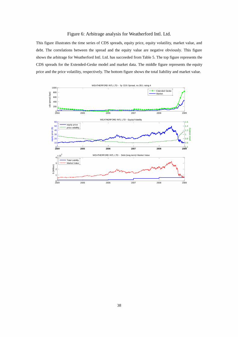
In contrast, the arbitrage for Weatherford Intl. Ltd. is relatively better. The

market spreads are overestimated after 2007, as shown in Fig. 6. The average of

market spread and model spread are 40 bps and 80 bps during 2007 to 2008,

respectively. After year 2008, the market and model spreads increase to 445 and 847

bps. The model spreads are approximately twice as large as the market spreads. If the

CDS spread and the equity price is in a divergence-divergence situation, the portfolio

will suffer substantial losses from both the position and the hedge, similar to the

arbitrage for Macy’s Inc. in Fig. 5. Conversely, the portfolio will make a substantial

amount of money in convergence-convergence situations, similar to the case of

Weatherford Intl. Ltd. in Fig. 6.

This research also analyzes arbitrage performance generated by simulated

trading to produce relevant statistics. In an early discussion, we mentioned that the

trigger of arbitrage trading is the minimum threshold to execute an arbitrage

automatically. To simplify our analysis, we set up three scenarios forand holding

period:=0.5, 1.0, and 2.0 and the holding is 30 days, 90 days, and 180 days. Nine

possible simulated strategies are implemented by the three different trading triggers,

20

combined with the three holding period assumptions. We assume that capital reserve

is unlimited, and no trades have to be liquidated early or for downside protection.

Tables 4 and 5 show the summary statistic of returns calculated based on nine

simulated strategies across every individual obligator during 2004 to 2008. Table 4

shows that the mean returns in most cases across different strategies are negative. The

largest loss case of 103% of negative return occurred on June 7, 2007, resulting from

a tremendous mispricing condition to permit simultaneous selling of CDS and equity.

This situation arose because the CDS spread increased from 51.2 bps to 101.1 bps,

and the stock price also increased from $39.15 to $41.99, which is meant for

divergence for both cases in conducting arbitrage strategies (=0.5, HP=30) over a

30-day holding period.

In contrast, from Table 5, the mean returns in most cases are positive, and the

largest profit case with 171% of positive return occurred on December 2, 2008,

resulting from a tremendous mispricing condition to permit simultaneous buying of

CDS and equity. The reason behind this scenario is that spread increased from 320

bps to 445 bps, and the stock price increased from $10.15 to $10.82. The enlarged

credit spreads and increased stock prices over a 30-day holding period resulted in a

significantly positive return.



7. Results

This section establishes a trading strategy to evaluate capital structure arbitrage

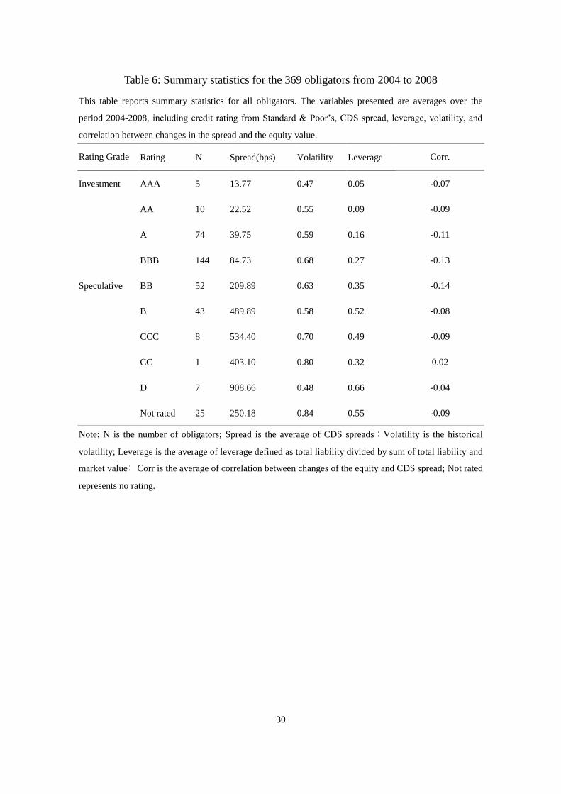
across all obligators from 2004 to 2008. Table 6 shows the summary statistics for all

obligators. The variables presented include credit rating from Standard & Poor’s,

21

CDS spread, leverage, volatility, and the correlation between CDS spread and equity

value. Table 6 shows that the correlations range from 2% to -14%. The average of all

correlations across obligators is -0.08.4 However, as shown in Table 6, a lower spread

is associated with a lower volatility and leverage, consistent with theoretical spread

predictions from CDS pricing models.

Table 7 shows the summary statistics of monthly returns based on nine simulated

strategies for all obligators. The results show that the strategies have a few

opportunities to produce positive mean returns for trading all obligators. The monthly

mean returns resulting from a trading trigger=0.5 are negative across all holding

periods. A longer holding period mean return gradually migrates to be negative and

the mean return for a larger trading trigger gradually turns to positive. Table 7 shows

that a lowertypically implies significant negative returns of arbitrage Minimum

mean returns are also relatively low across all strategies because of no downside

protection for liquidation.

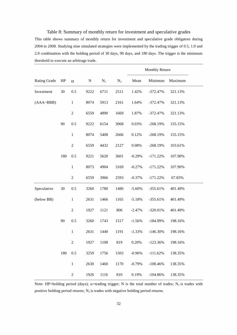
In Table 8, as trading strategies are implemented separately on investment-grade

and speculative-grade obligators, in most cases, the former produces positive mean

returns and the latter generates mostly negative mean returns. For investment-grade

obligators, a longer holding period leads to a lower mean return and most cases

produce a negative return within a 180-day holding period. The strategy of a short

holding period with a high trading trigger (HP=30,=2) yields monthly mean returns

of 1.87% for investment-grade obligators and -2.47% for speculative-grade obligators.

As shown in Table 6, speculative-grade obligators are less significant than

4 This is consistent with Yu (2006) and Currie and Morris (2002). Yu (2006) found that individual

correlations ranged from -5% to -15% according to different data sample periods, indicating that capital

structure arbitrage may be ineffective because of a weak correlation between the two markets.

22

investment-grade obligators in the correlation between equity and credit derivatives

markets. Therefore, low mean returns of arbitrage are predictable in the case of

speculative-grade obligators, where the effect is similar to the case of

investment-grade, despite the negative mean returns.

Arbitrage returns resulting from the extended Geske-Johnson model with

different trading strategies is similar to the results in Yu (2006). Capital structure

arbitrage between equity and credit derivatives markets is highly complex. Trading

with a larger trading trigger and a shorter holding period based on investment-grade

obligators is a seemingly profitable arbitrage. On the contrary, arbitrage with long

holding periods may suffer huge loss because the correlation between the equity

market and the credit derivatives market is insignificant and results in tremendous

mispricing.




8. Conclusion

This paper uses the extended Geske-Johnson model combined with different

trading strategies to evaluate capital structure arbitrage. The comparison between the

extended Geske-Johnson model and the CreditGrades model shows that both models

are similar in CDS spread calculation and are consistent with the market CDS spread.

However, the extended Geske-Johnson model with a multi-period debt structure can

predict default much earlier than the CreditGrades model in extreme cases, because

the extended Geske-Johnson model can exploit multi-period debt structure

information to predict the default probability of a company. In contrast, the

23

CreditGrades model only considers total liability as the reference to predict the default

probability of a company. Both models have different methodologies to deal with

corporate debt structures, and therefore different prediction power regarding the

default risk of a firm.

Debt structure is a key factor in driving a firm to default. This study is the first to

incorporate multi-period debt structures using the extended Geske-Johnson model to

predict CDS spread and evaluate capital structure arbitrage. Although the statistics

regarding arbitrage show an insignificant profit generated, there might still be room

for improvement if enhanced calibration methods can used to predict CDS spread or

default probability. The availability of more precise multi-period debt structure

information would allow the extended Geske-Johnson model to conduct arbitrage

strategies that are more appropriate, to become a more suitable tool to implement

capital structure arbitrage than the CreditGrades model.

24

References

Bajlum, C., and P.T. Larsen, 2008, “Capital structure arbitrage: model choice and

volatility calibration,” Working paper.

Berndt, A., R. Douglas, D. Duffie, M.Ferguson, and D. Schranz, 2004, “Measuring

default risk premia from default swap rates and EDFs,” Working paper,

Stanford University.

Black F., and M. Scholes, 1973, “The pricing of options and corporate liabilities,” The

Journal of Political Economy 81, 637-654.

Calamos, N., 2003, Convertible arbitrage: insights and techniques for successful

hedging, Wiley Finance.

Chatiras, M. and B. Mukherjee, 2004, “Capital Structure Arbitrage: An Empirical

Investigation Using Stocks and High Yield Bonds,” Working paper, University

of Massachusetts.

Chen, R.R., and S.K. Yeh, 2006, “Pricing credit default swaps with the extended

Geske-Johnson Model,” Working paper.

Currie, A., and J. Morris, 2002, “And now for capital structure arbitrage,” Euromoney

(December), 38-43.

Duarte, J., F. A. Longstaf, and F. Yu, 2005, “Risk and return in fixed income arbitrage:

Nickels in front of a steamroller?” Working paper, University of California.

Eom, Y., J. Helwege, and J. Huang, 2004, “Structural models of corporate bond

pricing: An empirical analysis,” Review of Financial Studies 17(2), 499-544.

Ericsson, J., J. Reneby, and H. Wang, 2005, “Can structural models price default risk?

Evidence from bond and credit derivative markets,” Working paper, McGill

University.

Geske R., 1977, “The valuation of corporate liabilities as compound options,” Journal

25

of Financial and Quantitative Analysis 5, 541-552.

Geske, R., and H. Johnson, 1984, “The valuation of corporate liabilities as compound

options: A correction,” Journal of Financial and Quantitative Analysis 19(2),

231-232.

Hogan, S., R. Jarrow, M. Teo, and M. Warachka, 2004, “Testing market efficiency

using statistical arbitrage with applications to momentum and value strategies,”

Journal of Financial Economics 73, 525-565.

Houweling, P., and T. Vorst, 2005, “Pricing default swap: empirical evidence,”

Journal of International Money and Finance 24, 1200-1225.

Jones, E., S. Mason, and E. Rosenfeld, 1984, “Contingent claims analysis of corporate

capital structures: An empirical investigation,” Journal of Finance 39,

611-627.

Leland, H. E., 1994, “Corporate debt value, bond covenants, and optimal capital

structure,” The Journal of Finance 49(4), 1213-1252.

Leland, H. E., and K. B. Toft, 1996, “Optimal capital structure, endogenous

bankruptcy, and the term structure of credit spreads,” The Journal of Finance

51(3), 987-1019.

Longstaff, F. A., S. Mithal, and E. Neis, 2005, “Corporate yield spreads: Default risk

or liquidity? new evidence from the credit default swap market,” The Journal

of Finance 60(5), 2213-2253.

Merton, R.C., 1974, “On the pricing of corporate debt: The risk structure of interest

rates,” Journal of Finance 29, 449-470, 1974.

Sepp, A., 2004, “Analytical Pricing of Double-Barrier Options under a Double

Exponential Jump Diffusion Process: Applications of Laplace Transform,”

International Journal of Theoretical and Applied Finance, 7(2), 151-175.

26

Visockis, R., 2011, “Capital Structure Arbitrage”, working paper.

Yu, F., 2006, “How Profitable Is Capital Structure Arbitrage?,” Financial Analysts

Journal 2006, Vol. 62, No.5, pp. 47-62.

27

Table 1: Definition of debt structure

This table presents the definition of six-period debt structure relative to the item description and

mnemonic of Compustat. All related debts are annual data, and the six-period debt structure can be

viewed as cash obligation at different year.

Item Description Mnemonic Item Number

Extended Geske model

Debt structure

Debt in Current Liabilities - Total DLC A34 1st period

Debt Due in 2nd Year DD2 A91 2nd period

Debt Due in 3rd Year DD3 A92 3rd period

Debt Due in 4th Year DD4 A93 4th period

Debt Due in 5th Year DD5 A94 5th period

Total Liabilities LT A181

Total Liabilities subtract the sum

of DLC,DD2, DD3,DD4 and DD5 6th period

Table 2: Input parameters of two pricing models

This table presents input parameters of two pricing models. The CreditGrades model uses total liability

and zero drift of asset value to derive the CDS spread from historical equity volatility. The extended

Gesek-Johnson model capture spread employs debt structure as cash obligations by a call option to

matching market firm’s equity in the multi-period behavior.

Model

Input Parameters

CreditGrades

(default barrier)

Extended

Geske-Johnson

( multi-period analysis)

Debt Total liability Debt structure

Equity Equity price Equity price

Equity Volatility rolling 1000-day

historical volatility

rolling 1000-day

historical volatility

Asset S+LD defined as model Matching equity by

model

Risk-free rate 5-year U.S. Treasury

yields

5-year U.S. Treasury

yields

Recovery rate 0.5 0.5

Standard deviation

of the default

barrier

0.3 none

28

Table 3: Summary statistics of the mispricing

This table reports summary statistics of the mispricing for all obligators based on CreditGrades and

extended Geske-Johnson models, respectively. The mispricing is defined as (actual spreads - model

spreads) The statistics are presented across the classification of grades, including investment and

speculative obligators.

Mean Median Std Max Min

CreditGrades

model

All -185 -79 539 3520 -7068

Investment -96 -53 145 178 -1961

Speculative -361 -215 864 3520 -7068

Extended

Geske-Johnson

model

All -60 11 324 1276 -2161

Investment -11 15 130 170 -1395

Speculative -217 -51 602 1276 -2161

Note: mispricing = market CDS spread – model CDS spread. Std is standard deviation. Unit: basis

points

Table 4: Holding period return for Macy’s Inc.

This table presents holding period return for Macy’s Inc based on nine simulated strategies during the

period 2004-2008. Each trade does not have to be liquidated early and to limited capital reserve.

Monthly Return

HP N N1 N2 Mean Minimum Maximum

30 0.5 48 22 26 -9.36% -103.00% 26.38%

1 38 17 21 -6.22% -91.90% 25.89%

2 17 7 10 -5.43% -39.43% 13.44%

90 0.5 48 24 24 -2.96% -40.35% 30.44%

1 38 22 16 -0.10% -40.35% 30.44%

2 17 10 7 0.44% -5.74% 7.17%

180 0.5 48 22 26 -3.70% -56.38% 9.81%

1 38 21 17 0.26% -11.35% 9.81%

2 17 8 9 0.66% -3.15% 5.34%

Note: HP=holding period (days); =trading trigger; N is the total number of trades; N1 is trades

with positive holding period returns; N2 is trades with negative holding period returns.

29

Table 5: Holding period return for Weatherford Intl. Ltd.

This table presents holding period return for Weatherford Intl Ltd based on nine simulated strategies

during the period 2004-2008. Each trade does not have to be liquidated early and to limited capital

reserve.

Monthly Return

HP N N1 N2 Mean Minimum Maximum

30 0.5 44 40 4 12.25% -21.79% 171.27%

1 25 22 3 14.30% -14.22% 171.27%

2 7 6 1 5.75% -12.34% 18.59%

90 0.5 44 35 9 4.85% -14.20% 31.18%

1 25 20 5 5.41% -6.80% 31.18%

2 7 3 4 -0.32% -6.80% 9.09%

180 0.5 44 31 13 0.73% -48.80% 9.53%

1 25 17 8 0.55% -48.80% 9.23%

2 7 1 6 -2.34% -5.61% 7.51%

Note: HP=holding period (days); =trading trigger; N is the total number of trades; N1 is trades

with positive holding period returns; N2 is trades with negative holding period returns.

30

Table 6: Summary statistics for the 369 obligators from 2004 to 2008

This table reports summary statistics for all obligators. The variables presented are averages over the

period 2004-2008, including credit rating from Standard & Poor’s, CDS spread, leverage, volatility, and

correlation between changes in the spread and the equity value.

Rating Grade Rating N Spread(bps) Volatility Leverage Corr.

-0.07

-0.09

-0.11

-0.13

-0.14

-0.08

-0.09

0.02

-0.04

-0.09

Investment AAA 5 13.77 0.47 0.05

AA 10 22.52 0.55 0.09

A 74 39.75 0.59 0.16

BBB 144 84.73 0.68 0.27

Speculative BB 52 209.89 0.63 0.35

B 43 489.89 0.58 0.52

CCC 8 534.40 0.70 0.49

CC 1 403.10 0.80 0.32

D 7 908.66 0.48 0.66

Not rated 25 250.18 0.84 0.55

Note: N is the number of obligators; Spread is the average of CDS spreads；Volatility is the historical

volatility; Leverage is the average of leverage defined as total liability divided by sum of total liability and

market value； Corr is the average of correlation between changes of the equity and CDS spread; Not rated

represents no rating.

31

Table 7: Summary of monthly return for statistic arbitrage

This table shows the summary statistic of monthly returns based on nine simulated

strategies for all obligators during 2004 to 2008. Studying nine simulated strategies were

implemented by the trading trigger of 0.5, 1.0 and 2.0 combination with the holding

period of 30 days, 90 days, and 180 days. The trigger is the minimum threshold to

execute an arbitrage trade.

Monthly Return

obligators HP N N1 N2 Mean Minimum Maximum

30 0.5 12442 8457 3985 -0.42% -372.47% 401.49%

1 10669 7349 3320 -0.04% -372.47% 401.49%

2 8457 5988 2469 0.87% -372.47% 401.49%

90 0.5 12442 7868 4574 -0.38% -268.19% 198.16%

1 10669 6823 3846 -0.21% -268.19% 198.16%

2 8457 5522 2935 0.13% -268.19% 198.16%

180 0.5 12440 7352 5088 -0.46% -171.22% 138.35%

1 10667 6344 4323 -0.38% -171.22% 138.35%

2 8456 5069 3387 -0.23% -171.22% 138.35%

Note: HP=holding period (days); =trading trigger; N is the total number of trades; N1 is

trades with positive holding period returns; N2 is trades with negative holding period

returns.

32

Table 8: Summary of monthly return for investment and speculative grades

This table shows summary of monthly return for investment and speculative grade obligators during

2004 to 2008. Studying nine simulated strategies were implemented by the trading trigger of 0.5, 1.0 and

2.0 combination with the holding period of 30 days, 90 days, and 180 days. The trigger is the minimum

threshold to execute an arbitrage trade.

Monthly Return

Rating Grade HP N N1 N2 Mean Minimum Maximum

Investment

(AAA~BBB)

30 0.5 9222 6711 2511 1.42% -372.47% 321.13%

1 8074 5913 2161 1.64% -372.47% 321.13%

2 6559 4890 1669 1.87% -372.47% 321.13%

90 0.5 9222 6154 3068 0.03% -268.19% 155.15%

1 8074 5408 2666 0.12% -268.19% 155.15%

2 6559 4432 2127 0.08% -268.19% 103.61%

180 0.5 9221 5620 3601 -0.29% -171.22% 107.90%

1 8073 4904 3169 -0.27% -171.22% 107.90%

2 6559 3966 2593 -0.37% -171.22% 67.83%

Speculative

(below BB)

30 0.5 3260 1780 1480 -5.60% -355.61% 401.49%

1 2631 1466 1165 -5.18% -355.61% 401.49%

2 1927 1121 806 -2.47% -320.01% 401.49%

90 0.5 3260 1743 1517 -1.56% -184.99% 198.16%

1 2631 1440 1191 -1.33% -146.30% 198.16%

2 1927 1108 819 0.20% -123.36% 198.16%

180 0.5 3259 1756 1503 -0.96% -111.62% 138.35%

1 2630 1460 1170 -0.79% -108.46% 138.35%

2 1926 1116 810 0.19% -104.86% 138.35%

Note: HP=holding period (days); =trading trigger; N is the total number of trades; N1 is trades with

positive holding period returns; N2 is trades with negative holding period returns.

33

Figure 1: The time-series of CDS spreads for Alcona Inc.

This figure depicts the spreads variation among market and models, the variation of equity price and

price volatility, and the variation of total liability and market equity. The top figure represents the CDS

spreads for different models and market data. The middle figure represents the equity price and the

price volatility, respectively. The bottom figure shows the total liability and market value.

2004 2005 2006 2007 2008 20090

500

1000

1500ALCOA INC - 5y CDS Spread, no.8, rating:4

cds s

pre

ad (

bps)

CreditGrades

Extended Geske

Market

2004 2005 2006 2007 2008 20090

10

20

30

40

50

60

equ

ity p

rice

($

)

ALCOA INC - Equity/Volatility

2004 2005 2006 2007 2008 20090.4

0.5

0.6

0.7

0.8

0.9

1

pri

ce

vo

latility

equity price

price volatility

2004 2005 2006 2007 2008 20090

1

2

3

4

5x 10

4ALCOA INC - Debt (long term)/ Market Value

$ (

Millio

n)

Total Liability

Market Value

34

Figure 2: The time-series of CDS spreads for Tenet Healthcare Corp.





2004 2005 2006 2007 2008 20090

500

1000

1500

2000TENET HEALTHCARE CORP - 5y CDS Spread, no.322, rating:6

cds s

pre

ad (

bps)

CreditGrades

Extended Geske

Market

2004 2005 2006 2007 2008 20090

10

20

equ

ity p

rice

($

)

TENET HEALTHCARE CORP - Equity/Volatility

2004 2005 2006 2007 2008 20090.5

1

1.5

pri

ce

vo

latility

equity price

price volatility

2004 2005 2006 2007 2008 20090

2000

4000

6000

8000

10000TENET HEALTHCARE CORP - Debt (long term)/ Market Value

$ (

Millio

n)

Total Liability

Market Value

35

Figure 3: The time-series of CDS spreads for Macy’s Inc.





2004 2005 2006 2007 2008 20090

500

1000

1500MACY'S INC - 5y CDS Spread, no.197, rating:5

cds s

pre

ad (

bps)

CreditGrades

Extended Geske

Market

2004 2005 2006 2007 2008 20090

10

20

30

40

50

60

equ

ity p

rice

($

)

MACY'S INC - Equity/Volatility

2004 2005 2006 2007 2008 20090.4

0.5

0.6

0.7

0.8

0.9

1

pri

ce

vo

latility

equity price

price volatility

2004 2005 2006 2007 2008 20090

0.5

1

1.5

2

2.5x 10

4MACY'S INC - Debt (long term)/ Market Value

$ (

Millio

n)

Total Liability

Market Value

36

Figure 4: The time-series of CDS spreads for Avis Budget Group Inc.





2004 2005 2006 2007 2008 20090

2000

4000

6000

8000

10000AVIS BUDGET GROUP INC - 5y CDS Spread, no.30, rating:7

cds s

pre

ad (

bps)

CreditGrades

Extended Geske

Market

2004 2005 2006 2007 2008 20090

5

10

15

20

25

30

35

40

equ

ity p

rice

($

)

AVIS BUDGET GROUP INC - Equity/Volatility

2004 2005 2006 2007 2008 20090.4

0.6

0.8

1

1.2

1.4

1.6

1.8

2

pri

ce

vo

latility

equity price

price volatility

2004 2005 2006 2007 2008 20090

0.5

1

1.5

2

2.5x 10

4AVIS BUDGET GROUP INC - Debt (long term)/ Market Value

$ (

Millio

n)

Total Liability

Market Value

37

Figure 5: Arbitrage analysis for Macy’s Inc.

This figure illustrates the time series of CDS spreads, equity price, equity volatility, market value, and

debt. The correlations between the spread and the equity value are negative obviously. This figure

shows mostly the negative mean return in different strategies for Macy’s Inc. from Table 4, although

the model CDS spreads line on the both sides of the market CDS spread. The top figure represents the

CDS spreads for the Extended-Geske model and market data. The middle figure represents the equity

price and the price volatility, respectively. The bottom figure shows the total liability and market value.

2004 2005 2006 2007 2008 20090

500

1000

1500MACY'S INC - 5y CDS Spread, no.197, rating:5

cds s

pre

ad (

bps)

Extended Geske

Market

2004 2005 2006 2007 2008 20090

10

20

30

40

50

60

equ

ity p

rice

($

)

MACY'S INC - Equity/Volatility

2004 2005 2006 2007 2008 20090.4

0.5

0.6

0.7

0.8

0.9

1

pri

ce

vo

latility

equity price

price volatility

2004 2005 2006 2007 2008 20090

0.5

1

1.5

2

2.5x 10

4MACY'S INC - Debt (long term)/ Market Value

$ (

Millio

n)

Total Liability

Market Value

38

Figure 6: Arbitrage analysis for Weatherford Intl. Ltd.

This figure illustrates the time series of CDS spreads, equity price, equity volatility, market value, and

debt. The correlations between the spread and the equity value are negative obviously. This figure

shows the arbitrage for Weatherford Intl. Ltd. has succeeded from Table 5. The top figure represents the

CDS spreads for the Extended-Geske model and market data. The middle figure represents the equity

price and the price volatility, respectively. The bottom figure shows the total liability and market value.

2004 2005 2006 2007 2008 20090

200

400

600

800

1000WEATHERFORD INTL LTD - 5y CDS Spread, no.353, rating:4

cds s

pre

ad (

bps)

Extended Geske

Market

2004 2005 2006 2007 2008 20090

10

20

30

40

50

60

equ

ity p

rice

($

)

WEATHERFORD INTL LTD - Equity/Volatility

2004 2005 2006 2007 2008 20090.4

0.6

0.8

1

1.2

1.4

1.6

pri

ce

vo

latility

equity price

price volatility

2004 2005 2006 2007 2008 20090

1

2

3

4x 10

4WEATHERFORD INTL LTD - Debt (long term)/ Market Value

$ (

Millio

n)

Total Liability

Market Value

Documents

Evaluation of Conducting Capital Structure Arbitrage …centerforpbbefr.rutgers.edu/2012PBFEAM/papers/020...Evaluation of Conducting Capital Structure Arbitrage Using the Multi-Period