Setting Up a Bayesian Analysis, WinbugsCoding Tricks, and CODA

Carrie Groth (Caroline)PUBH 7440: Spring 2015

March 26, 2015

1

Preview

General AnnouncementsPicking groups for the final projectSetting up a Bayesian Analysis

Problem 19 Set-upWinbugs Coding Tricks

Zeros TrickOnes Trick (Used for Problem 20)Other Tricks?

CODA

2

Picking Groups for the Final Project

Groups of 2-3 people

3

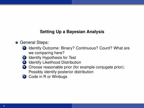
Setting Up a Bayesian Analysis

General Steps:1 Identify Outcome: Binary? Continuous? Count? What are

we comparing here?2 Identify Hypothesis for Test3 Identify Likelihood Distribution4 Choose reasonable prior (for example conjugate prior);

Possibly identify posterior distribution5 Code in R or Winbugs

4

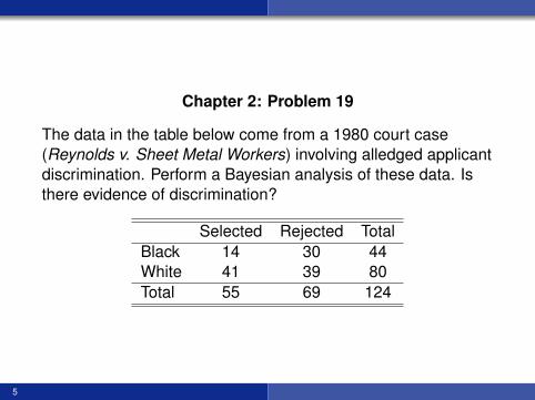
Chapter 2: Problem 19

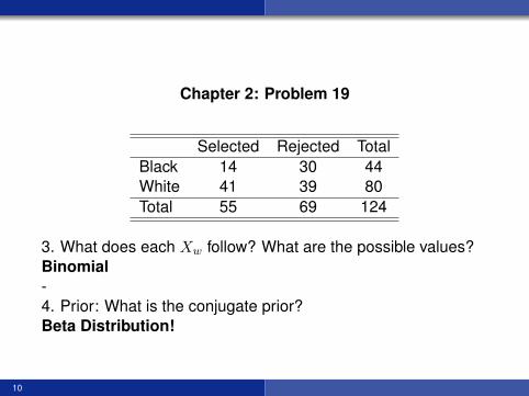
The data in the table below come from a 1980 court case(Reynolds v. Sheet Metal Workers) involving alledged applicantdiscrimination. Perform a Bayesian analysis of these data. Isthere evidence of discrimination?

Selected Rejected TotalBlack 14 30 44White 41 39 80Total 55 69 124

5

Chapter 2: Problem 19

Selected Rejected TotalBlack 14 30 44White 41 39 80Total 55 69 124

1. Primary Outcome (Consider 124 to be fixed)?What is 14/44? What are we comparing that too?

6

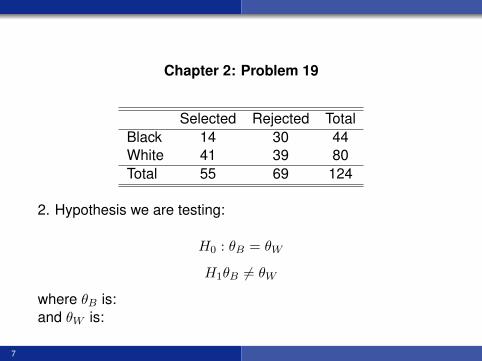
Chapter 2: Problem 19

Selected Rejected TotalBlack 14 30 44White 41 39 80Total 55 69 124

2. Hypothesis we are testing:

H0 : θB = θW

H1θB 6= θW

where θB is:and θW is:

7

Chapter 2: Problem 19

Selected Rejected TotalBlack 14 30 44White 41 39 80Total 55 69 124

3. What does each Xw follow? What are the possible values?

8

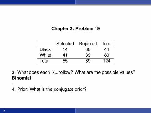
Chapter 2: Problem 19

Selected Rejected TotalBlack 14 30 44White 41 39 80Total 55 69 124

3. What does each Xw follow? What are the possible values?Binomial-4. Prior: What is the conjugate prior?

9

Chapter 2: Problem 19

Selected Rejected TotalBlack 14 30 44White 41 39 80Total 55 69 124

3. What does each Xw follow? What are the possible values?Binomial-4. Prior: What is the conjugate prior?Beta Distribution!

10

Chapter 2: Problem 19

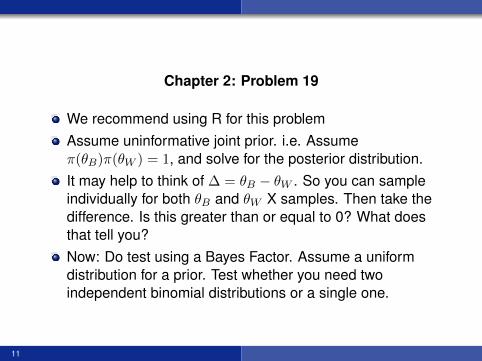
We recommend using R for this problemAssume uninformative joint prior. i.e. Assumeπ(θB)π(θW ) = 1, and solve for the posterior distribution.It may help to think of ∆ = θB − θW . So you can sampleindividually for both θB and θW X samples. Then take thedifference. Is this greater than or equal to 0? What doesthat tell you?Now: Do test using a Bayes Factor. Assume a uniformdistribution for a prior. Test whether you need twoindependent binomial distributions or a single one.

11

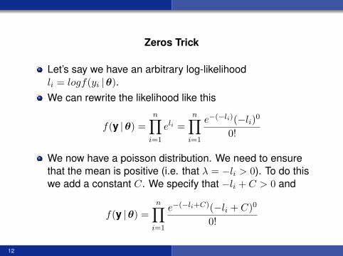
Zeros Trick

Let’s say we have an arbitrary log-likelihoodli = logf(yi |θ).We can rewrite the likelihood like this

f(y |θ) =

n∏i=1

eli =

n∏i=1

e−(−li)(−li)0

0!

We now have a poisson distribution. We need to ensurethat the mean is positive (i.e. that λ = −li > 0). To do thiswe add a constant C. We specify that −li + C > 0 and

f(y |θ) =

n∏i=1

e−(−li+C)(−li + C)0

0!

12

Zeros Trick in Winbugs

C<-10000for(i in 1:n){zeros[i]<-0zeros[i]~dpois(zeros.mean[i])zeros.mean[i]<- -l[i]+ Cl[i]<- #Log Likelihood function...}

13

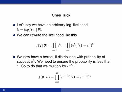
Ones Trick

Let’s say we have an arbitrary log-likelihoodli = logf(yi |θ).We can rewrite the likelihood like this

f(y |θ) =

n∏i=1

eli =

n∏i=1

(eli)1(1− eli)0

We now have a bernoulli distribution with probability ofsuccess eli . We need to ensure the probability is less than1. So to do that we multiply by e−C :

f(y |θ) =

n∏i=1

(eli−C)1(1− eli−C)0

14

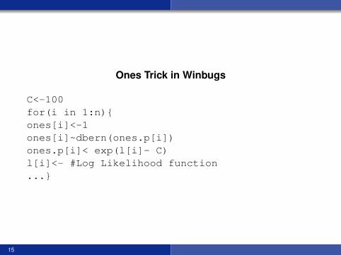
Ones Trick in Winbugs

C<-100for(i in 1:n){ones[i]<-1ones[i]~dbern(ones.p[i])ones.p[i]< exp(l[i]- C)l[i]<- #Log Likelihood function...}

15

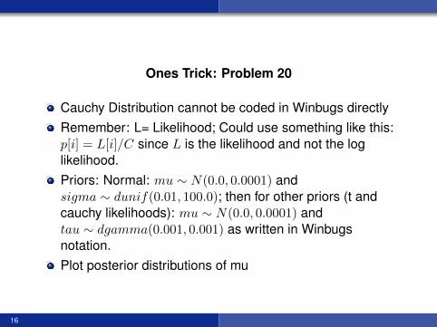
Ones Trick: Problem 20

Cauchy Distribution cannot be coded in Winbugs directlyRemember: L= Likelihood; Could use something like this:p[i] = L[i]/C since L is the likelihood and not the loglikelihood.Priors: Normal: mu ∼ N(0.0, 0.0001) andsigma ∼ dunif(0.01, 100.0); then for other priors (t andcauchy likelihoods): mu ∼ N(0.0, 0.0001) andtau ∼ dgamma(0.001, 0.001) as written in Winbugsnotation.Plot posterior distributions of mu

16

CODA

A very important R package used in Bayesian analysisExample:2.16: Stack Loss

17

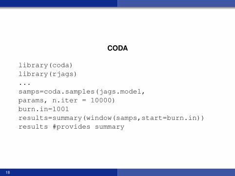
CODA

library(coda)library(rjags)...samps=coda.samples(jags.model,params, n.iter = 10000)burn.in=1001results=summary(window(samps,start=burn.in))results #provides summary

18

Gelman Rubin Diagnostic

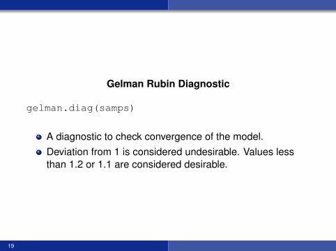
gelman.diag(samps)

A diagnostic to check convergence of the model.Deviation from 1 is considered undesirable. Values lessthan 1.2 or 1.1 are considered desirable.

19

Trace Plots

traceplot(samps[,#])

A plot that allows one to assess mixing of the chainsMixing: When chains intertwineA graphical assessment of convergence

20

Effective Sample Size

effectiveSize(samps[,#])

Deals with the autocorrelationNumber of independent samples (after taking into accountautocorrelation)

21

Autocorrelation Plots

autocorr.plot(samps[,1])

Plots the autocorrelation vs. the lagAutocorrelation, as defined by Wikapedia, is the “similaritybetween observations as a function of the time lagbetween them"

22

References

Bayesian Methods for Data Analysis, Third Edition byBradley P. Carlin and Thomas A. Louis Chapter 2http://www.biostat.umn.edu/ dipankar/pubh7440/codes/0-1-Trick.pdfhttp://cran.r-project.org/web/packages/coda/coda.pdf

23