Bayesian Inference Using WBDev: A Tutorial for Social ...winbugs-development.mrc-bsu.cam.ac.uk/files/wbdev_tutorial.pdfBayesian Inference Using WBDev: A Tutorial for Social Scientists

Bayesian Inference Using WBDev:A Tutorial for Social Scientists

Ruud Wetzels1, Michael D. Lee2, and Eric–Jan Wagenmakers1

1 University of Amsterdam2University of California, Irvine

Correspondence concerning this article should be addressed to:Ruud Wetzels

University of Amsterdam, Department of PsychologyRoetersstraat 15

1018 WB Amsterdam, The NetherlandsPh: (+31) 20–525–8871Fax: (+31) 20–639–0279

E–mail may be sent to [email protected].

Abstract

Over the last decade, the popularity of Bayesian data analysis in the em-pirical sciences has greatly increased. This is partly due to the availabilityof WinBUGS—a free and flexible statistical software package that comeswith an array of predefined functions and distributions—allowing users tobuild complex models with ease. For many applications in the psycholog-ical sciences, however, it is highly desirable to be able to define one’s owndistributions and functions. This functionality is available through the Win-BUGS Development Interface (WBDev). This tutorial illustrates the use ofWBDev by means of concrete examples, featuring the Expectancy–Valencemodel for risky behavior in decision–making, and the shifted Wald distribu-tion of response times in speeded choice.

Keywords: WinBUGS, WBDev, BlackBox, Bayesian Modeling

Introduction

Psychologists who seek quantitative models for their data face formidable challenges.Not only are data often noisy and scarce, but they may also have a hierarchical structure,they may be partly missing, they may have been obtained under an ill–defined samplingplan, and they may be contaminated by a process that is not of interest. In addition,

A WBDEV TUTORIAL 2

the models under consideration may have multiple restrictions on the parameter space,especially when there is useful prior information about the subject matter at hand.

In order to address these kinds of real–world challenges, the psychological scienceshave started to use Bayesian models for the analysis of their data (e.g., Lee, 2008; Rouder& Lu, 2005; Hoijtink, Klugkist, & Boelen, 2008). In Bayesian models, existing knowledge isquantified by prior probability distributions and updated upon consideration of new data toyield posterior probability distributions. Modern approaches to Bayesian inference includeMarkov chain Monte Carlo sampling techniques (MCMC; e.g., Gamerman & Lopes, 2006;Gilks, Richardson, & Spiegelhalter, 1996) and these allow researchers to construct proba-bilistic models that respect the complexities in the data, allowing almost any probabilisticmodel to be evaluated against data.

One of the most influential software packages for MCMC–based Bayesian inference isknown as WinBUGS (BUGS stands for Bayesian inference Using Gibbs Sampling; Cowles,2004; Sheu & O’Curry, 1998; Lunn, Thomas, Best, & Spiegelhalter, 2000; Ntzoufras, 2009).WinBUGS comes equipped with an array of predefined functions (e.g., sqrt for square rootand sin for sine) and distributions (e.g., the Binomial and the Normal) that allow users tocombine these elementary building blocks into complex probabilistic models almost at will.

For some psychological modeling applications, however, it is highly desirable to defineone’s own functions and distributions. In particular, user–defined functions and distribu-tions greatly facilitate the use of psychological process model such as the Attention Learn-ing Covering map (ALCOVE; Kruschke, 1992), the Generalized Context Model for categorylearning (GCM; Nosofsky, 1986), the Expectancy–Valence model for decision–making (Buse-meyer & Stout, 2002), the SIMPLE model of memory (Brown, Neath, & Chater, 2007), orthe Ratcliff diffusion model of response times (Ratcliff, 1978).

The ability to implement these user–defined functions and distributions can beachieved through the use of the WinBUGS Development Interface (WBDev; Lunn, 2003),an add–on program that allows the user to hand–code functions and distributions in Com-ponent Pascal (e.g., http://en.wikipedia.org/wiki/Component_Pascal). The use ofWBDev brings several advantages. For instance, complicated WBDev components leadto faster computation than their counterparts programmed in straight WinBUGS code.Moreover, some models will only work properly when implemented in WBDev. Anotheradvantage of WBDev is that it compartmentalizes the code, resulting in scripts that areeasier to understand, communicate, adjust, and debug. A final advantage of WBDev isthat it allows the user to program functions and distributions that are simply not availablein WinBUGS, but may be central components of psychological models (Donkin, Averell,Brown, & Heathcote, in press; Vandekerckhove, Tuerlinckx, & Lee, 2009).

This tutorial aims to stimulate psychologists to use WBDev by providing four thor-oughly documented examples; for both functions and distributions, we provide a simple anda more complex example. All examples are relevant to psychological research.1 Our tuto-rial assumes no programming experience and is intended to be accessible to psychologicalscientists.

1There already exists a concise tutorial on how to write a function and how to write a distribution. The

tutorials are written by David Lunn and Chris Jackson and they come with software for writing code in

WBDev. However, these examples require advanced programming skills and they are not directly relevant

for psychologists.

A WBDEV TUTORIAL 3

We start by discussing the WBDev implementation of a simple function that involvesthe addition of variables. We then turn to the implementation of a complicated function thatinvolves the Expectancy–Valence model (Busemeyer & Stout, 2002; Wetzels, Vandekerck-hove, Tuerlinckx, & Wagenmakers, in press). Next, we discuss the WBDev implementationof a simple distribution, first focusing on the Binomial distribution, and then turning to theimplementation of a more complicated distribution that involves the shifted Wald distribu-tion (Heathcote, 2004; Schwarz, 2001). For all of these examples, we explain the crucialparts of the WBDev scripts and the WinBUGS code. The thoroughly commented code isavailable online at www.ruudwetzels.com and in the appendix. For each example, our ex-planation of the WBDev code is followed by application to data and the graphical analysisof the output.

Installing WBDev (Blackbox)

Before we can begin hard–coding our own functions and distributions we need todownload and install three programs; WinBUGS, WBDev and BlackBox.2 To make sureall programs function properly, they have to be installed in the order given below.

1. Install WinBUGS

WinBUGS is the core program that we will use. Download the latestversion from http://www.mrc-bsu.cam.ac.uk/bugs/winbugs/contents.shtml (Win-BUGS14.exe). Install the program in the default directory ./Program Files/WinBUGS14.Make sure to register the software by obtaining the registration key and following theinstructions—WinBUGS will not work without it.

2. Install WinBUGS Development Interface (WBDev)

Download WBDev from http://www.winbugsdevelopment.org.uk/ (WBDev.exe).Unzip the executable in your WinBUGS directory ./Program Files/WinBUGS14. Thenstart WinBUGS, open the“wbdev01 09 04.txt” file and follow the instructions at the topof the file. During the process, WBDev will create its own directory /WinBUGS14/WBDev.

3. Install BlackBox Component Builder

BlackBox is a development environment for programs written in Component Pascaland this includes WinBUGS. Blackbox can be downloaded from http://www.oberon.ch/

blackbox.html. At the time of writing, the latest version is 1.5. Install Blackbox inthe default directory: ./Program Files/BlackBox Component Builder 1.5. Go to theWinBUGS directory and select all files (press “Ctrl–A”) and copy them (press “Ctrl+C”).Next, open the BlackBox directory and paste the copied files in there (press “Ctrl+V”).Select “ Yes to all” if asked about replacing files. Once this is done, you will be able toopen BlackBox and run WinBUGS from inside Blackbox. This completes installation ofthe software, and we can start to write our own functions and distributions.

2At the time of writing, all programs are available without charge.

A WBDEV TUTORIAL 4

Functions

The mathematical concept of a function expresses a dependence between variables.The basic idea is that some variables are given (the input) and with them, other variablesare calculated (the output). Sometimes, complex models require many arithmetic opera-tions to be performed on the data. Because such calculations can become computationallydemanding using straight WinBUGS code, it can be convenient to use WBDev and imple-ment these calculations as a function. The first part of this section will explain a problemwithout using WBDev. We then show how to use WBDev to program a simple and a morecomplex function.

Example 1: A Rate Problem

A binary process has two possible outcomes. It might be that something eitherhappens or does not happen, or that something either succeeds or fails, or takes one valuerather than the other. An inference that often is important for these sorts of processesconcerns the underlying rate at which the process takes one value rather than the other.Inferences about the rate can be made by observing how many times the process takes eachvalue over a number of trials.

Suppose that someone plays a simple card game and can either win or lose. Weare interested in the probability that the player wins a game. To study this problem, weformalize it by assuming the player plays n games and wins k of them. These are known, orobserved, data. The unknown variable of interest is the probability θ that the player winsany one specific game. Assuming the games are statistically independent (i.e., that whathappened on one game does not influence the others, so that the probability of winning isthe same for all of the games), the number of wins k follows a Binomial distribution, whichis written as

k ∼ Binomial(

θ, n)

(1)

and can be read “the success count k out of a total of n trials is Binomially distributedwith success rate θ”. In this example, we will assume a success count of 9 (k = 9) and atrial total of 10 (n = 10).

A rate problem: the model file. A so–called model file is used to implement the modelinto WinBUGS. The model file for inferring θ from an observed n and k looks like this:

model

{

# prior on the rate parameter theta

theta ~ dunif(0,1)

# observed wins k out of total games n

k ~ dbin(theta,n)

}

The twiddles symbol (∼) means “is distributed as”. Because we use a Uniform distri-bution between 0 and 1 as a prior on the rate parameter θ, we write theta ∼ dunif(0,1).

A WBDEV TUTORIAL 5

This indicates that, a priori, each value of θ is equally likely. Furthermore, k is Binomiallydistributed with parameters θ and n (i.e., k ∼ dbin(theta,n)). Note that dunif anddbin are two of the predefined distributions in WinBUGS. The hash symbol (#) is used forcomments. The lines starting with this symbol are not executed by WinBUGS.

Copy the text into an empty file and save it as “model rateproblemfunction.txt” inthe directory from where you want to work. From this point, there are various ways inwhich to proceed. One way is to work from within WinBUGS; another way is to controlWinBUGS calling it from a more general purpose program. Here, we use R (a statistical pro-gramming language)3 to call WinBUGS, but widely–used alternative research programmingenvironments such as MATLAB are also available (Lee & Wagenmakers, in preparation).

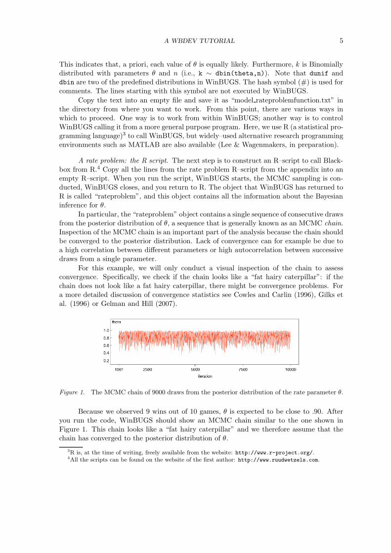
A rate problem: the R script. The next step is to construct an R–script to call Black-box from R.4 Copy all the lines from the rate problem R–script from the appendix into anempty R–script. When you run the script, WinBUGS starts, the MCMC sampling is con-ducted, WinBUGS closes, and you return to R. The object that WinBUGS has returned toR is called “rateproblem”, and this object contains all the information about the Bayesianinference for θ.

In particular, the “rateproblem” object contains a single sequence of consecutive drawsfrom the posterior distribution of θ, a sequence that is generally known as an MCMC chain.Inspection of the MCMC chain is an important part of the analysis because the chain shouldbe converged to the posterior distribution. Lack of convergence can for example be due toa high correlation between different parameters or high autocorrelation between successivedraws from a single parameter.

For this example, we will only conduct a visual inspection of the chain to assessconvergence. Specifically, we check if the chain looks like a “fat hairy caterpillar”: if thechain does not look like a fat hairy caterpillar, there might be convergence problems. Fora more detailed discussion of convergence statistics see Cowles and Carlin (1996), Gilks etal. (1996) or Gelman and Hill (2007).

Figure 1. The MCMC chain of 9000 draws from the posterior distribution of the rate parameter θ.

Because we observed 9 wins out of 10 games, θ is expected to be close to .90. Afteryou run the code, WinBUGS should show an MCMC chain similar to the one shown inFigure 1. This chain looks like a “fat hairy caterpillar” and we therefore assume that thechain has converged to the posterior distribution of θ.

3R is, at the time of writing, freely available from the website: http://www.r-project.org/.4All the scripts can be found on the website of the first author: http://www.ruudwetzels.com.

A WBDEV TUTORIAL 6

Figure 2. The posterior distribution of the rate parameter θ after observing 9 wins out of 10 games.The dashed gray line indicates the mode of the posterior distribution at θ = .90. The 95% confidenceinterval extends from .59 to .98.

We use the samples from Figure 1 to estimate the posterior distribution of θ. Toarrive at the posterior distribution, the samples are not plotted as a time series but as adistribution. In order to estimate the posterior distribution of θ, we applied the standarddensity estimator in R. Figure 2 shows that the mode of the distribution is very close to .90,just as we expected. The posterior distribution is relatively spread out over the parameterspace, the 95% confidence interval extends from .59 to .98. This indicates the uncertaintyabout the value of θ. Had we observed 900 wins out of a total of 1000 games the posteriorof θ would be much more concentrated around the mode of .90, as our knowledge about thetrue value of θ would have greatly increased.

Example 2: ObservedPlus

In this section we examine the rate problem again, but now we change the variables.Specifically, we design a function that adds 1 to the number of observed wins, and 10 tothe number of total games. So, when we use k = 9 and n = 10 as before, we end up with

knew = kold + 1 = 9 + 1 = 10 (2)

and

nnew = nold + 10 = 10 + 10 = 20. (3)

Hence, when we use our new function, the mode of the posterior distribution should nolonger be .90 but .50 (10/20 = .50). To obtain these results, we are going to build afunction called “ObservedPlus”, using the template “VectorTemplate.odc”. This templateis located in the folder “...\BlackBoxComponentBuilder1.5\WBdev\Mod”.

ObservedPlus: the WBDev script. The online script file shows text in three colors.The parts that are colored black should not be changed. The parts in red are comments andthese are not executed by Blackbox. The parts in blue are the most relevant parts of thecode, because these are the parts that can be changed to create the desired function. The

A WBDEV TUTORIAL 7

templates for writing the functions and distributions in this tutorial come together with theWBDev software and were written by David Lunn and Chris Jackson.5

We now give a detailed explanation of the ObservedPlus WBDev function. Thenumbers (*X*) correspond to the numbers in the ObservedPlus WBDev script. For thissimple example, we show some crucial parts of the WBDev scripts below. In the otherexamples throughout the article, we only describe the crucial parts of the code.

(*1*) MODULE WBDevObservedPlus;

The name of the module is typed here. We have named our module ObservedPlus.The name of the module (so the part after MODULE WBDev...) has to start with acapital letter.

(*2*) args := "ss";

Here you must define specific arguments about the input of the function. Youcan choose between scalars (s) and vectors (v). A scalar means that the input isa single number. When you want to use a variable that consists of more numbers(for example a time series) you need a vector. This line has to correspond withthe constants defined at (*3*). In our example, we use two scalars, the number ofsuccesses k and the total number of observations n.

(*3*) in = 0; ik = 1;

Because of what has been defined at (*2*), WBDev already knows that thereshould be two variables here. We name them in and ik, with in at the first spot(with number 0) and ik at the second spot (with number 1). WBDev always startscounting at 0 and not at 1.

Note that we did not name our variables n and k, but in and ik. This is because itis more insightful to use n and k later on, and it is not possible to give two or morevariables the same name. Finally, note that the positions of the constants correspondto the positions of the input of the variables into the function in the model file. Wewill return to this issue later.

(*4*) n, k: INTEGER;

The variables that are used in the calculations need to be defined. Both vari-ables are defined as integers, because the Binomial distribution only allows integersas input: counts of successes and the total games that are played can only be positiveintegers.

(*5*) n := SHORT(ENTIER(func.arguments[in][0].Value()));

k := SHORT(ENTIER(func.arguments[ik][0].Value()));

5The homepage of David Lunn is http://www.mrc-bsu.cam.ac.uk/BSUsite/AboutUs/People/davidl.

xml, the homepage of Chris Jackson is http://www.mrc-bsu.cam.ac.uk/BSUsite/AboutUs/People/chris/

chris_Research.shtml.

A WBDEV TUTORIAL 8

This code takes the input values (in and ik) and gives them a name. We de-fined two variables in (*4*), and we are now going to use them. What the scriptsays here is: take the input values in and ik and store them in the integer variablesn and k. Because the input variables are not automatically assumed to be integers,we have to transform them and make sure the program recognizes them as integers.So, in other words, the first line says that n is the same as the first input variable ofthe function (see Figure 3), and the second line says that k is the same as the secondinput variable of the function.

Figure 3. A detailed explanation of part (*5*) of “ObservedPlus.odc”.

(*6*) n:=n+10;

k:=k+1;

values[0] := n;

values[1] := k;

This is the part of the script where we do the actual calculations. At the endof this part, we fill the output array values with the new n and k.

(*7*) END WBDevObservedPlus.

The last thing that needs to be done is to make sure that the name of themodule at the end is the same as the name at the top of the file. The last line has toend with a period. Hence, the last line of the script is ENDWBDevObservedPlus..

Now you need to compile the function by pressing “Ctrl–k”. Syntax errors causeWBDev to return an error message. Name this file “ObservedPlus.odc” and save it in thedirectory “...\BlackBoxComponentBuilder1.5\WBdev\Mod”.

We are not entirely ready to use the function yet. WBDev needs to know thatthere exists a function called ObservedPlus; WBDev also needs to know what the inputlooks like (i.e., how many inputs are there, what order are they presented, and are theyscalars and vectors?), and what the output is. To accomplish this, open the file “func-tions.odc” in the directory “...\BlackBoxComponentBuilder1.5\WBdev\Rsrc”. Add the

A WBDEV TUTORIAL 9

line: v<-"ObservedPlus"(s,s) "WBDevObservedPlus.Install" and then save the file.The next time that WBDev is started, it knows that there is a function named Observed-Plus which has two scalars as input, and a vector as output. The function is now ready tobe used in a model file.

ObservedPlus: the model file. In order to use the newly scripted function Observed-Plus we use a model file that is similar to the model file used in the earlier rate problemexample.

model

{

# Uniform prior on the rate parameter

theta ~ dunif(0,1)

# use the function to get the new n and the new k

data[1:2] <- ObservedPlus(n,k)

# define the new n and new k as variables

newn <- data[1]

newk <- data[2]

# the new observed data

newk ~ dbin(theta,newn)

}

We assume a Uniform prior on θ (i.e., theta ∼ dunif(0,1)). The function Ob-servedPlus takes as input the total number of games n and the number of wins k. Fromthem, the new n and new k can be calculated (i.e., data[1:2] <- ObservedPlus(n,k)).Note that functions require the use of the assignment operator (<-) instead of the twiddlessymbol (∼). Remember that in the WBDev function the location of in was 0 and thelocation of ik was 1. Because that order was used, the input has to have n first and then k.

Next, newn is the first number in the vector data and newk is the second (i.e., newn <-

data[1], newk <- data[2]). Remember that when scripting in WBDev, the first elementhas index 0, but in the model file the first element has index 1. Finally, we use our newvariables to do inference on the rate parameter θ (i.e., newk ∼ dbin(theta,newn)).

Copy the text from the model file into an empty text file and name this file“model observedplus.txt”. Copy this file to the location of the model file that was usedin the rate problem example.

ObservedPlus: the R script. To run this model from R, we can use the script of theoriginal rate problem. The only thing that needs to be changed is the name of the model file.This should now be “model observedplus.txt”. Change this name and run the R–script.

After you run the code, WinBUGS should show an MCMC chain similar to the oneshown in Figure 4. The chain looks like a fat hairy caterpillar, so for now we assume it hasconverged to the posterior distribution of θ.

Figure 5 shows the posterior distribution of θ. The mode of the distribution is .50,because knew = 10 and nnew = 20. Again, because the total number of games played is fairly

A WBDEV TUTORIAL 10

Figure 4. The MCMC chain of 9000 draws from the posterior distribution of θ, after using thefunction ObservedPlus.

Figure 5. The posterior distribution of the rate parameter θ, after using the function ObservedPlus.The dashed gray line indicates the mode of the posterior distribution at θ = .50. The 95% confidenceinterval extends from .30 to .70.

small, the posterior distribution of θ is relatively spread out (the 95% confidence intervalranges from .30 to .70), reflecting our uncertainty about the true value of θ.

Example 3: The Expectancy–Valence Model

In the example described above, we could have used plain WinBUGS code instead ofwriting a script in Blackbox. But sometimes it can be very useful to write a Blackbox scriptinstead of plain WinBUGS code, especially if the model under consideration is relativelycomplex. Implementing such a model into WBDev can speed up the computation time forinference substantially. The present example, featuring the Exptectancy–Valence model tounderstand risk–seeking behavior in decision making, provides a concrete demonstration ofthis general point.

Suppose a psychologist wants to study decision making of clinical populations undercontrolled conditions. A task that is often used for this purpose is the “Iowa gamblingtask”, developed by Bechara and Damasio (IGT; Bechara, Damasio, Damasio, & Anderson,1994; Bechara, Damasio, Tranel, & Damasio, 1997).

In the IGT, participants have to discover, through trial and error, the differencebetween risky and safe decisions. In the computerized version of the IGT, the participant

A WBDEV TUTORIAL 11

starts with $2000 in play money. The computer screen shows players four decks of cards(A, B, C, and D), and then they have to select a card from one of the decks. Each card isassociated with either a reward or a loss. The default payoff scheme is presented in Table 1.

Bad Decks Good Decks

A B C D

reward per trial 100 100 50 50number of losses per 10 cards 5 1 5 1loss per 10 cards 1250 1250 250 250net profit per 10 cards −250 −250 250 250

Table 1: Rewards and Losses in the IGT. Cards from decks A and B yield higher rewards than cardsfrom decks C and D, but they also yield higher losses. The net profit is highest for cards from decksC and D.

At the start of the IGT, participants are told that they should maximize net profit.During the task, they are presented with a running tally of the net profit, and the taskfinishes after 250 card selections.

The Expectancy–Valence (EV) model proposes that choice behavior in the IGT comesabout through the interaction of three latent psychological processes. Each of these pro-cesses is vital to producing successful performance, typified by an increase in preference forthe good decks over the bad decks with increasing experience. First, the model assumesthat the participant, after selecting a card from deck k, k ∈ {1, 2, 3, 4} on trial t, calculatesthe resulting net profit or valence. This valence vk is a combination of the experiencedreward W (t) and the experienced loss L(t):

vk(t) = (1 − w)W (t) + wL(t). (4)

Thus, the first parameter of the Expectancy Valence model is w, the attention weight forlosses relative to rewards, w ∈ [0, 1].

On the basis of the sequence of valences vk experienced in the past, the participantforms an expectation Evk of the valence for deck k. In order to learn, new valences needto update the expected valence Evk. If the experienced valence vk is higher or lower thanexpected, Evk needs to be adjusted upward or downward, respectively. This intuition iscaptured by the equation

Evk(t + 1) = Evk(t) + a(vk(t) − Evk(t)), (5)

in which the updating rate a ∈ [0, 1] determines the impact of recently experienced valences.The EV model also uses a reinforcement learning method called softmax selection or

Boltzmann exploration (Kaelbling, Littman, & Moore, 1996; Luce, 1959) to account for thefact that participants initially explore the decks, and only after a certain number of trialsdecide to always prefer the deck with the highest expected valence.

Pr[Sk(t + 1)] =exp (θ(t)Evk)

∑

4

j=1exp (θ(t)Evj)

. (6)

A WBDEV TUTORIAL 12

In this equation, 1/θ(t) is the “temperature” at trial t and Pr(Sk) is the probability ofselecting a card from deck k. In the EV model, the temperature is assumed to vary withthe number of observations according to

θ(t) = (t/10)c, (7)

where c is the response consistency or sensitivity parameter. In fits to data, this parameteris usually constrained to the interval [−5, 5]. When c is positive, response consistency θincreases (i.e., the temperature 1/θ decreases) with the number of observations. This meansthat choices will be more and more guided by the expected valences. When c is negative,choices will become more and more random as the number of card selections increases.

In sum, the EV model decomposes choice behavior in the Iowa gambling task in threecomponents or parameters:

1. An attention weight parameter w that quantifies the weighting of losses versus rewards.

2. An updating rate parameter a that quantifies the memory for rewards and losses.

3. A response consistency parameter c that quantifies the level of exploration.

The EV model: the WBDev script. To implement the EV model as a function inWBDev it is useful to first describe what data is observed and passed on to WinBUGS.In this example, we examine the data of one participant who has completed a 250–trialIGT. Hence, the observed data are an index of which deck was chosen at each trial, and thesequence of wins and losses that the participant incurred.

To construct the WBDev script we use the template called “VectorTemplate.odc”again. As in the last example, only the blue parts in the text can be altered.

(*1*) The name of the module is typed here. We want to name our module EV. The nameof the module (so the part after MODULE WBDev...) has to start with a capitalletter.

(*2*) This line has to correspond with the constants at (*3*). In the EV example, weuse 3 scalars for the 3 parameters and 3 vectors for the wins, losses and index at eachtrial.

(*3*) The input of the function needs to defined here. We begin with the data vectors(the order is arbitrary, but needs to correspond to the one used in the model file) andwe name these constants iwins, ilosses and iindex. After that, the function has asinput the parameters of the EV–model, iw, ia and ic.

(*4*) In this section we define all the variables that we need to use in our calculations.

(*5*) Here we take our input EV parameters and assign them to the variables that wedefined in part (*4*).

(*6*) This is the part of the script where we do the actual calculations. At the end of thispart, we fill the output variable called “values”, with the output of our EV–function,the probability of choice for a deck.

A WBDEV TUTORIAL 13

(*7*) The last thing that needs to be done is to make sure that the name of the module atthe end is the same as the name at the top of the file. The last line has to end witha period.

Now you need to compile the function by pressing “Ctrl–k”. Syntax errors causeWBDev to return an error message. Name this file “EV.odc” and save it in the directory“...\BlackBoxComponentBuilder1.5\WBdev\Mod”.

We need to add this function to the function file (like in the ObservedPlus example)so that WinBUGS knows that the EV function exists, the next time it is started. Open thefile“functions.odc” in the directory “...\ BlackBox Component Builder 1.5\ WBdev\ Rsrc”.Add the line: v <- "EV"(v,v,v,s,s,s) "WBDevEV.Install" and then save the file. Thenext time that WBDev is started, it knows that there is a function named EV which hasthree vectors and three scalars as input, and a vector as output. The function is now readyto be used in a model file.

The EV–model: the model file. In order to use the EV–model we need to implementthe graphical model in WinBUGS. The following model file is used in this example:

model

{

# EV parameters are assigned prior distributions

w ~ dunif(0,1)

a ~ dunif(0,1)

c ~ dunif(-5,5)

# data from the EV function

evprobs[1:1000] <- EV(wi[],lo[],ind[],w,a,c)

# only use the information from the chosen deck

# see explanation below

for (i in 1:250)

{

p.EV[i,1] <- evprobs[deckA[i]]

p.EV[i,2] <- evprobs[deckB[i]]

p.EV[i,3] <- evprobs[deckC[i]]

p.EV[i,4] <- evprobs[deckD[i]]

ind[i] ~ dcat(p.EV[i,])

}

}

The parameters of the model, w, a, c are assigned Uniform prior distributions. w anda are bounded between 0 and 1 and c is bounded between -5 and 5 (i.e., w ∼ dunif(0,1), a

∼ dunif(0,1), c ∼ dunif(-5,5)). The wins and the losses from the 250–trials are storedin the vectors wi and lo. The indices from the decks that were chosen are stored in the vectorind. Together with the EV parameters they are input for the EV function that calculatesthe probability per choice (i.e., evprobs[1:1000] <- EV(wi[],lo[],ind[],w,a,c)).

Note that this function calculates 1000 probabilities for a 250–trial dataset. This isbecause the probability for each deck is calculated, not only for the chosen deck but for all

A WBDEV TUTORIAL 14

decks. So at each trial, four probabilities are calculated and for 250 trials this totals 1000probabilities. However, we are only interested in the probability of the chosen deck.

To handle this problem, we make four vectors, deckA, deckB, deckC and deckD whichare rows of length 250. Each vector contains a sequence of numbers where the number atposition t is calculated by adding four to the number at position t− 1 (xt = xt−1 + 4). Thevector deckA starts with number 1, deckB starts with number 2, deckC starts with number3 and deckD starts with number 4. Using these vectors, we can disentangle the probabilitiesfor each deck at each trial, evprobs[deckA[i]] corresponds to the probabilities of choosingdeck 1 at each trial i, evprobs[deckB[i]] to the probabilities of choosing deck 2 at eachtrial i, evprobs[deckC[i]] to the probabilities of choosing deck 3 at each trial i andevprobs[deckD[i]] to the probabilities of choosing deck 4 at each trial.

Finally, we state that the choice for a deck at trial i (the observed data vector ind) isCategorically distributed (i.e., ind[i] ∼ dcat(p.EV[i,])). The Categorical distributionis the probability distribution for the choice of a card deck. This distribution is a general-ization of the Bernoulli distribution for a categorical random variable. (i.e., the choice forone of the four decks at each trial of the IGT). Copy the text from the model into an emptyfile and save it as “model ev.txt” in the directory from where you want to work.

The EV model: the R script.

To run this model and to supply WinBUGS with the data, we use the R–script givenin the appendix. Copy the script from the appendix and change the working directory tothe directory where the model file is located. This script contains fictitious data from aperson who completed a 250–trial IGT.6 After you run the code, WinBUGS should showthree MCMC chains similar to the ones shown in Figure 6.

Figure 6. Three MCMC chains of 9000 draws each for the three EV parameters, the attentionweight parameter w, the updating rate parameter a and response consistency parameter c.

6The data can be downloaded from www.ruudwetzels.com.

A WBDEV TUTORIAL 15

For all the EV–parameters, the chains look like fat hairy caterpillars and hence appearto have converged to the posterior distribution. Because the EV–parameters are slightlyharder to estimate than the rate parameters from the earlier examples —due to the com-plexity of the EV–model— we have to make sure that we are sampling from the correctposterior distribution of w, a and c.

Besides visual inspection of the MCMC chain, we now compute the often used measureof convergence, the R̂ (Rhat) statistic (Gelman, Carlin, Stern, & Rubin, 2004, pp. 295–297).Rhat allows the user to compare the within– to between–chain variance from the sampledvalues, and then provides an easy–to–interpret measure of whether independent chains haveconverged to sample from the same distribution. After convergence, Rhat should be veryclose to 1 (at least smaller than 1.1). Note that Rhat can never be lower than 1.

To check for convergence, we run three chains, with all three having a different startingposition, and then calculate Rhat. In this example, we observe that for each EV–parameter,the chains have converged properly (Rhat ≈ 1). Note that it is important that the chainsfor all parameters have converged.

Figure 7. The posterior distributions of the three EV parameters, w, a and c. The dashed graylines indicate the modes of the posterior distributions at w = .43, a = .25 and c = 0.58. The 95%confidence intervals for w, a and c extend from .38 to .57, from .17 to .36 and from 0.31 to 0.74,respectively.

After having assured ourselves that the chains have converged we can plot the resultingposterior distributions. Figure 7 shows that the posterior mode of the attention weightparameter w is .43, the posterior mode of the update parameter a is .25 and the posteriormode of the consistency parameter c is 0.58.

On an average computer, it takes about 85 seconds to generate these chains. Had wehave used plain WinBUGS instead of WBDev code to compute these chains, the calculationtime would have taken approximately 15 minutes. Hence, implementing the function intoWBDev speeds up the analysis by a factor 10. However, the speed up is not the onlyadvantage of implementing functions into WBDev. Sometimes, complex models will onlywork properly when implemented in WBDev. Another advantage of WBDev is that itcompartmentalizes the code, resulting in scripts that are easier to understand, communicate,adjust, and debug.

A WBDEV TUTORIAL 16

Distributions

Statistical distributions are invaluable in psychological research. For example, inthe simple rate problem discussed earlier, we use the Binomial distribution to model ourdata. WinBUGS comes equipped with an array of predefined distributions, but it doesnot include all distributions that are potentially useful for psychological modeling. UsingWBDev, researchers can augment WinBUGS to include these desired distributions.

In the next section we will explain how to write a new distribution, starting with theBinomial distribution as a simple introduction, and then considering the more complicatedshifted Wald distribution.

Example 4: Binomial distribution

Obviously, the Binomial distribution is already hard–coded in WinBUGS. But, be-cause it is a very well–known and relatively simple distribution, it serves as a useful firstexample.

To program a distribution in WBDev, we can use the distribution templatethat is already in the Blackbox directory. This file is located in the folder:“...\BlackBoxComponentBuilder1.5\WBdev\Mod”. In order to program the distribu-tion, we first need to write out the log likelihood function:

log (Pr(K = k)) = log (f(k;n, θ))

= log

((

n

k

)

θk(1 − θ)n−k

)

= log

((

n

k

)

+ log(θk) + log(1 − θ)n−k

)

= log(n!) − log(k!) − log(n − k)! + k log(θ) + (n − k) log(1 − θ).

(8)

Binomial distribution: the WBDev script. Please see the appendix for the WBDevcode of the Binomial distribution.

(*1*) The name of the module is typed here. We want to name our module BinomialTest.The name of the module (so the part after MODULE WBDev...) has to start with acapital letter.

(*2*) The parameters of the input of the Binomial distribution, theta and n.

(*3*) Here global variables can be declared. With global is meant that it is loaded onlyonce, while the value of the variable may be needed many times. This part of thetemplate does not need to be changed for this example.

(*4*) We have to declare what type of arguments are the input of the distribution. In thiscase these are two scalars (i.e. two single numbers), theta and n.

(*5*) This describes whether the distribution is discrete or continuous. When the dis-tribution is discrete, isDiscrete should be set to TRUE. When the distribution iscontinuous, it should be set to FALSE. For the Binomial distribution isDiscrete is setto TRUE.

A WBDEV TUTORIAL 17

The other thing that is defined in this part of the script is if the cumulative distributionis to be provided. If so, canIntegrate should be set to TRUE. If this is set to true, analgorithm should be provided at (*11*). We set canIntegrate to FALSE because wedid not implement the cumulative distribution.

(*6*) This part of the code should define the natural bounds of the distribution. In ourcase, we take 0 as a lower bound and n as an upper bound, because k can never belarger than n.

(*7*) As the name implies, this part is the part where the full log likelihood of the dis-tribution is defined. This is an implementation of the log likelihood as defined inEquation 8.

(*8*) Sometimes WinBUGS can ignore the normalizing constants. When that is the case,WinBUGS calls LogPropLikelihood(.). In our example, we refer back to the full loglikelihood function.

(*9*) Occasionally, WinBUGS can make use of the LogPrior(.) procedure, which is pro-portional to the real log–prior function. In other words, this procedure omits theadditive constants on the log scale. In our example, we just refer back to the full loglikelihood function.

(*10*) This is the part where the cumulative distribution is defined when in part (*7*)canIntegrate is set to TRUE. Because we set this to FALSE, we do not define anythingin this section.

(*11*) The DrawSample(.) procedure returns a pseudo–random number from the newdistribution. We do not use this function, because we do not need to draw valuesfrom the new distribution. You would have to do this when you have missing values.

(*12*) The last thing that needs to be done is to make sure that the name of the moduleat the end is the same as the name at the top of the file. The last line has to end witha period.

Now you need to compile the function by pressing “Ctrl–k”. Syntax errors cause WBDevto return an error message. Save this file as “BinomialTest.odc” and copy this file into theappropriate blackbox directory, “...\BlackBoxComponentBuilder1.5\WBdev\Mod”.

Open the distribution file “distributions.odc” in the directory “...\ BlackBoxComponent Builder 1.5\ WBdev\ Rsrc”. Add the line s ∼ "BinomialTest"(s,s)

"WBDevBinomialTest.Install" and then save it. The next time you start Blackbox, theprogram will know that there exists a distribution called BinomialTest, and that the inputsare two scalars (single numbers).

Binomial distribution: the model file. To use the scripted Binomial distribution, wewrite a model file that is very similar to the model file used in the rate problem example.We only need to change the name of the distribution from dbin to BinomialTest.

A WBDEV TUTORIAL 18

model

{

# prior on rate parameter theta

theta~dunif(0,1)

# observed wins k out of total games n

k~BinomialTest(theta,n)

}

This example is essentially the same statistical problem as the first example, therate problem. Ten games are played (i.e., n = 10) and nine games are won (i.e., k = 9).We assume a Uniform prior on θ (i.e., theta ∼ dunif(0,1)). The observed wins k aredistributed as our newly made BinomialTest with rate parameter theta and total gamesn (i.e., k∼BinomialTest(theta,n)). With theta and k defined, this completes the modelfor BinomialTest. Save this file as “model rateproblemdistribution.txt” and copy it to yourworking directory.

Binomial distribution: the R script. The last thing that we need to do is to start Rand copy the code from the appropriate R–script from the appendix into R. Change theworking directory to the directory where your modelfile is located. After you run the code,the results should be similar to those shown in Figure 1 and Figure 2.

The shifted Wald distribution

Many psychological models use response times (RTs) to infer latent psychologicalproperties and processes (Luce, 1986). One common distribution used to model RTs isthe inverse Gaussian or Wald distribution (Wald, 1947). This distribution represents thedensity of the first passage times of a Wiener diffusion process toward a single absorbingboundary, as shown in Figure 8, using three parameters.

The parameter v reflects the drift rate of the diffusion process. The parameter areflects the separation between the starting point of the diffusion process and the absorbingbarrier. The third parameter, Ter, is a positive–valued parameter that shifts the entiredistribution. The probability density function for this shifted Wald distribution is given by:

f(t|v, a, Ter) =a

√

2π(t − Ter)3exp

{

−[a − v(t − Ter)]

2

2(t − Ter)

}

, (9)

which is unimodel and positively skewed. Because of these qualitative properties, it is agood candidate for fitting empirical RT distributions. As an illustration, Figure 9 showschanges in the shape of the shifted Wald distribution as a result of changes in the shiftedWald parameters v, a, and Ter.

The shifted Wald parameters have a clear psychological interpretation (e.g., Heath-cote, 2004; Luce, 1986; Schwarz, 2001, 2002). Participants are assumed to accumulate noisyinformation until a predefined threshold amount is reached and a response is initiated. Driftrate v quantifies task difficulty or subject ability, response criterion a quantifies response

A WBDEV TUTORIAL 19

Figure 8. A diffusion process with one boundary. The shifted Wald parameter a reflects theseparation between the starting point of the diffusion process and the absorbing barrier, v reflectsthe drift rate of the diffusion process and Ter is a positive–valued parameter that shifts the entiredistribution.

Figure 9. Changes in the shape of the shifted Wald distribution as a result of changes in theparameters v, a and Ter. Each panel shows the shifted Wald distribution with different combinationsof parameters.

caution, and the shift parameter Ter quantifies the time needed for non–decision processes(Matzke & Wagenmakers, in press). Experimental paradigms in psychology for which itis likely that there is only a single absorbing boundary include saccadic eye movementtasks with few errors (Carpenter & Williams, 1995), go/no–go tasks (Gomez, Ratcliff, &Perea, 2007) or simple reaction time tasks (Luce, 1986, pp. 51–57). Here we show how toimplement the shifted Wald distribution in WBDev.

Shifted Wald distribution: the WBDev script. Please see the appendix for the WBDevcode. Open Blackbox, and save the content of this part of the appendix to a new file. Namethis file “ShiftedWald.odc”.

(*1*) The name of the module is typed here. We want to name our module ShiftedWald.The name of the module (so the part after MODULE WBDev...) has to start with acapital letter.

A WBDEV TUTORIAL 20

(*2*) The parameters of the distribution, which, in this case are the drift rate v, responsecaution a and shift Ter.

(*3*) Here global variables can be declared. A global variable is loaded only once, but thevalue of the variable is usually needed many times.

(*4*) We have to declare what type of arguments are the input of the distribution. In thiscase these are the three scalar parameters of the shifted Wald distribution.

(*5*) This part of the code describes whether samples from the distribution are discreteor continuous. When the distribution is discrete, isDiscrete should be set to TRUE.When the distribution is continuous, it should be set to FALSE. For the shifted–Walddistribution isDiscrete is FALSE.

The other this part of the script defines is whether the cumulative distribution is tobe provided. If so, canIntegrate should be set to TRUE. If this is set to true, analgorithm should be provided at (*11*). We set canIntegrate to FALSE because wedid not implement the cumulative distribution.

(*6*) This part of the code should define the natural bounds of the distribution. In ourcase, we take Ter as a lower bound and INF (meaning +∞) as an upper bound.

(*7*) As the name implies, this part is the part where the full log likelihood of the distri-bution is defined.

(*8*) Sometimes WinBUGS can ignore the normalizing constants. When that is the case,WinBUGS calls LogPropLikelihood(.). In our example, we refer back to the full loglikelihood function.

(*9*) Occasionally, WinBUGS can make use of the LogPrior(.) procedure, which is pro-portional to the real log–prior function. In other words, this procedure omits theadditive constants on the log scale. In our example, we just refer back to the full loglikelihood function.

(*10*) Here the cumulative distribution can be defined in case canIntegrate at (*7*) hadbeen set to TRUE. Because we have set canIntegrate to FALSE, we do not defineanything in this section.

(*11*) The DrawSample(.) procedure returns a pseudo–random number from the newdistribution. We do not use this function, because we do not need to draw valuesfrom the new distribution. You would have to do this when you have missing values.

(*12*) The last thing that needs to be done is to make sure that the name of the moduleat the end is the same as the name at the top of the file. The last line has to end witha period.

Now you need to compile the function by pressing “Ctrl–k”. Syntax errors cause WBDevto return an error message. Save this file as “ShiftedWald.odc” and copy this file into theappropriate blackbox directory, “...\BlackBoxComponentBuilder1.5\WBdev\Mod”.

A WBDEV TUTORIAL 21

Open the distribution file “distributions.odc” in the directory “...\ BlackBoxComponent Builder 1.5\ WBdev\ Rsrc”. Add the line s ∼ "ShiftedWald"(s,s,s)

"WBDevShiftedWald.Install" and then save it. The next time you start Blackbox, theprogram will know that there exists a distribution called ShiftedWald, and that the inputsare three scalars (single numbers).

The shifted Wald distribution: the model file. Once we implemented the WBDevfunction in blackbox, we can use the function ShiftedWald in the model. The model file isas follows:

model

{

# prior distributions for shifted Wald parameters

# drift rate

v ~ dunif(0,10)

# boundary separation

a ~ dunif(0,10)

# Non-decision time

Ter ~ dunif(0,1)

# data are shifted Wald distributed

for (i in 1:nrt)

{

rt[i] ~ ShiftedWald(v,a,Ter)

}

}

The priors for v and a, are Uniform distributions that range from 0 to 10 (i.e., v

∼ dunif(0,10), i.e., a ∼ dunif(0,10)). The prior for Ter is a Uniform distributionthat ranges from 0 to 1 (i.e., Ter ∼ dunif(0,1). With the priors in place, we can use ourShiftedWald function to estimate the posterior distributions for the three model parametersv, a and Ter (i.e., rt[i] ∼ ShiftedWald(v,a,Ter)). Save the lines as a text file and nameit “model shiftedwaldind.txt”.

Shifted Wald distribution: the R script. Now, copy the R–script into an R–file andrun it. Change the directory of the location of the model file and the location of your copyof Blackbox to the appropriate directories. The R–script loads a real dataset from a lexicaldecision task (Wagenmakers, Ratcliff, Gomez, & McKoon, 2008). Nineteen participantshad to quickly decide whether a visually presented letter string was a word (e.g., table) or anonword (e.g., drapa). We will fit the response times of correct “word” responses of the firstparticipant to the shifted Wald distribution. The response time data can be downloadedfrom www.ruudwetzels.com. After you run the code, WinBUGS should show an MCMCchain similar to the one shown in Figure 10.

The chains do not look like fat hairy caterpillars. They seem to have a lot of freedomto move around the parameter space, so we cannot be certain that the chains have converged

A WBDEV TUTORIAL 22

Figure 10. The MCMC chains of of the marginal posteriors of all three individual Wald parameters,v, a and Ter.

properly. To assess convergence more formally, we ran three chains using different startingpoints for each chain. Next, we calculated Rhat to check whether the chains have convergedto the same stationary distribution. For each parameter, Rhat is smaller than 1.1, so wecan tentatively assume that the chains have converged.

Figure 11. The posterior distribution of the three Wald parameters v, a and Ter. The dashed graylines indicate the modes of the posterior distributions at v = 5.57, a = 1.09 and Ter = .33. The 95%confidence intervals for v, a and Ter extend from 4.12 to 8.00, from 0.80 to 3.52 and from .09 to .36,respectively.

Figure 11 shows the posterior distribution of the three shifted Wald parameters, v, aand Ter. One thing that stands out is that the posterior distributions of the shifted Waldparameters are very spread out across the parameter space. The 95% confidence intervalsfor v, a and Ter extend from 4.12 to 8.00, from 0.80 to 3.52 and from .09 to .36, respectively.It seems that data from only one participant are not enough to yield very accurate estimatesof the shifted Wald parameters. In the following section we show how our estimates willimprove when we use a hierarchical model and analyze all participants simultaneously.

A WBDEV TUTORIAL 23

Shifted Wald distribution: a hierarchical extension. In an experimental setting, theproblem of few data per participant can be addressed by hierarchical modeling (Farrell &Ludwig, 2008; Gelman & Hill, 2007; Rouder, Sun, Speckman, Lu, & Zhou, 2003; Shiffrin,Lee, Wagenmakers, & Kim, 2008). In our shifted Wald example, each subject is assumed togenerate their data according to the shifted Wald distribution, but with different parametervalues. We extend the individual analysis and assume that the parameters for each subjectare chosen from a Normal distribution. This means that all individual participants areassumed to have their shifted Wald parameters drawn from the same group distribution,allowing all the data provided by all the partipants to be used for inferring parametervalues, without making the unrealistic assumption that participants are identical copies ofeach other.

The model file that implements the hierarchical shifted Wald analysis is shown below:

model

{

# prior distributions for group means:

v.g ~ dunif(0,10)

a.g ~ dunif(0,10)

Ter.g ~ dunif(0,1)

# prior distributions for group standard deviations:

sd.v.g ~ dunif(0,5)

sd.a.g ~ dunif(0,5)

sd.Ter.g ~ dunif(0,1)

# transformation from group standard deviations to group

# precisions (i.e., 1/var, which is what WinBUGS expects

# as input to the dnorm distribution):

lambda.v.g <- pow(sd.v.g,-2)

lambda.a.g <- pow(sd.a.g,-2)

lambda.Ter.g <- pow(sd.Ter.g,-2)

# data come From a shifted Wald distribution

for (i in 1:ns) #subject loop

{

# individual parameters drawn from group level

# normals censored to be positive using the

# I(0,) command:

v.i[i] ~ dnorm(v.g,lambda.v.g)I(0,)

a.i[i] ~ dnorm(a.g,lambda.a.g)I(0,)

Ter.i[i] ~ dnorm(Ter.g,lambda.Ter.g)I(0,)

# for each participant,

# data are shifted Wald distributed

for (j in 1:nrt[i])

{

rt[i,j] ~ ShiftedWald(v.i[i],a.i[i],Ter.i[i])

}

}

}

A WBDEV TUTORIAL 24

The hierarchical analysis of the reaction time data proceeds as follows. Theprior for the group means is a Uniform distribution, ranging from 0 to 10 (i.e., v.g

∼ dunif(0,10), a.g ∼ dunif(0,10)) or from 0 to 1 (i.e., Ter.g ∼ dunif(0,1)).The standard deviations are drawn from a Uniform distribution ranging from 0to 5 (i.e., sd.v.g ∼ dunif(0,5), sd.a.g ∼ dunif(0,5)) or from 0 to 1 (i.e.,sd.Ter.g ∼ dunif(0,5)). Next, the standard deviations have to be transformedto precisions (i.e., lambda.v.g <- pow(sd.v.g,-2), lambda.a.g <- pow(sd.a.g,-2),

lambda.Ter.g <- pow(sd.Ter.g,-2)). Then, the individual parameters v.i, a.i andTer.i are drawn from Normal distributions with corresponding group means andgroup precisions (i.e., v.i[i]∼dnorm(v.g,lambda.v.g)I(0,), a.i[i] ∼ dnorm(a.g,

lambda.a.g)I(0,), Ter.i[i] ∼ dnorm(Ter.g, lambda.Ter.g)I(0,)). For each in-dividual, the data are distributed according to a shifted Wald distribution withtheir own individual parameters. Save the model file as a text file and name it:“model shiftedwaldhier.txt”.

When we run this model using the R–script for the hierarchical analysis, we first focuson the group mean parameters v.g, a.g and Ter.g. Figure 12 shows the MCMC chains fromthe three shifted Wald parameters. To check for convergence, we ran three chains, with allthree having a different starting position, and then calculate Rhat. The chains appear tohave converged, an impression that is supported by Rhat values close to 1 (Rhat for Ter.g,a.g and v.g is approximately 1.).

Figure 12. Three chains, consisting of 9000 MCMC draws each, from the posterior distributions ofthe three “group–level” shifted Wald parameters, v.g, a.g and Ter.g.

Figure 13 shows the posterior distributions of the shifted Wald group–mean parame-ters. The distributions indicate that there is relatively little uncertainty about the parametervalues. The posterior distributions of the group–mean parameters are concentrated aroundtheir modes v.g = 4.27, a.g = 0.97 and Ter.g = 0.36. The 95% confidence intervals for v.g,a.g and Ter.g extend from 3.80 to 4.70, from 0.85 to 1.10 and from .34 to .38, respectively.

It is informative to consider the influence of the hierarchical extension on the indi-

A WBDEV TUTORIAL 25

Figure 13. The posterior distribution of the three “group–level” shifted Wald parameters v.g, a.gand Ter.g. The dashed gray lines indicate the modes of the posterior distributions at v.g = 4.27,a.g = .97 and Ter.g = .36. The 95% confidence intervals for v.g, a.g and Ter.g extend from 3.80 to4.70, from 0.85 to 1.10 and from .34 to .38, respectively.

vidual estimates for the shifted Wald parameters. Specifically, we can examine the MCMCchains for the same subject that we analyzed in the individual shifted Wald analysis, butnow in the hierarchical setting.

Figure 14. The MCMC chains of of the marginal posteriors of all three individual Wald parameters,v, a and Ter, analyzed using a hierarchical model.

After you run the R–script for the hierarchical analysis of the shifted Wald example,WinBUGS should show three MCMC chains similar to the ones shown in Figure 14. Thechains are better behaved than the chains from the individual analysis (Figure 10). Thehierarchical extension leads to a practical improvement, through faster convergence for thecomputational MCMC estimation process. However, the hierarchical extension also leads toa theoretical improvement because compared to the individual analysis, the chains appearmuch less diffuse. This shows that the hierarchical model leads to a better understandingof the model parameters.

A WBDEV TUTORIAL 26

Figure 15. The posterior distribution of the three individual shifted Wald parameters v.i, a.i andTer.i from the hierarchical analysis (solid lines) and the individual analysis (dotted lines). Thedashed gray lines indicate the modes of the posterior distributions from the hierarchical analysisat v.i[1] = 4.57, a.i[1] = 0.96 and Ter.i[1] = .34. The 95% confidence intervals in the hierarchicalmodel for v.i[1], a.i[1] and Ter.i[1] extend from 3.86 to 5.49, from 0.75 to 1.24 and from .31 to.37,respectively.

To underscore this point, Figure 15 shows the posterior distributions of the individualshifted Wald parameters, for both the hierarchical analysis and the individual analysis. Itis clear that the posterior distributions of the shifted Wald parameters are less spread outin the hierarchical analysis than in the individual analysis. Also, the parameter estimatesfrom the hierarchical analysis are slightly different than those from the individual analysis.More precisely, they seem to have moved towards their common group mean. This effect iscalled shrinkage, and is a standard and important property of hierarchical models (Gelmanet al., 2004).

In sum, the WBDev implementation of the shifted Wald distribution enables re-searchers to infer shifted Wald parameters from reaction time data. Not only does Win-BUGS allow straightforward analyses on individual data, it also makes it easy to add hi-erarchical structure to the model. This can greatly improve the quality of the posteriorestimates, and is often a very sensible and informative way of analyzing data.

Discussion

In this paper we have shown how the WinBUGS Development Interface (WBDev)can be used to help psychological scientists model their sparse, noisy, but richly structureddata. We have shown how a relatively complex function such as the Expectancy–Valencemodel can be incorporated in a fully Bayesian analysis of data. Furthermore, we haveshown how to implement statistical distributions, such as the shifted Wald distribution,that have specific application in psychological modeling, but are not part of a standard setof statistical distributions.

The WBDev program is set up for Bayesian modeling, and is equipped with mod-ern sampling techniques such as Markov chain Monte Carlo. These sampling techniquesallow researchers to construct quantitative Bayesian models that are non–linear, highlystructured, and potentially very complicated. The advantages of using WBDev togetherwith WinBUGS are substantial. WinBUGS code can sometimes lead to slow computationand complex models might not work at all. In addition, scripting some components of themodel in WBDev can speed up the computation time considerably. Furthermore, compart-

A WBDEV TUTORIAL 27

mentalizing the scripts can make the model easier to understand and debug. Moreover,WinBUGS facilitates statistical communication between researchers who are interested inthe same model. The most basic advantage, however, is that WBDev allows the user toprogram functions and distributions that are simply unavailable in WinBUGS.

Once a core psychological model is implemented in WBDev, it is straightforwardto take into account variability across participants or items, using a hierarchical, multi–level extension (i.e., models with random effect for subjects or items). This approachallows a researcher to model individual differences as smooth variations in parameters ofa certain cognitive model, and allows for different groups of subjects to use fundamentallydifferent cognitive models as well. That way, we can capture a broad range of between–group differences and also the within–group difference at the same time, all within onestatistical procedure. This eliminates the problem of different groups within one subjectspool, it is a way to handle contaminants in the data and it gives more insight in the data.For these reasons, we think the fully Bayesian analysis of highly structured models is likelyto be a driving force behind future theoretical and empirical progress in the psychologicalsciences.

References

Bechara, A., Damasio, A. R., Damasio, H., & Anderson, S. (1994). Insensitivity to future conse-quences following damage to human prefrontal cortex. Cognition, 50, 7–15.

Bechara, A., Damasio, H., Tranel, D., & Damasio, A. R. (1997). Deciding advantageously beforeknowing the advantageous strategy. Science, 275, 1293–1295.

Brown, G., Neath, I., & Chater, N.(2007). A temporal ratio model of memory. Psychological Review,114, 539–576.

Busemeyer, J. R., & Stout, J. C. (2002). A contribution of cognitive decision models to clinical as-sessment: Decomposing performance on the Bechara gambling task. Psychological Assessment,14, 253–262.

Carpenter, R. H. S., & Williams, M. L. L.(1995). Neural computation of log likelihood in control ofsaccadic eye movements. Nature, 377, 59–62.

Cowles, M. K.(2004). Review of WinBUGS 1.4. The American Statistician, 58, 330–336.

Cowles, M. K., & Carlin, B. P. (1996). Markov chain Monte Carlo convergence diagnostics: Acomparative review. Journal of the American Statistical Association, 883–904.

Donkin, C., Averell, L., Brown, S., & Heathcote, A.(in press). Getting more from accuracy and re-sponse time data: Methods for fitting the linear ballistic accumulator model. Behavior ResearchMethods.

Farrell, S., & Ludwig, C. (2008). Bayesian and maximum likelihood estimation of hierarchicalresponse time models. Psychonomic Bulletin & Review, 15, 1209–1217.

Gamerman, D., & Lopes, H. F. (2006). Markov chain Monte Carlo: Stochastic simulation forBayesian inference. Boca Raton, FL: Chapman & Hall/CRC.

Gelman, A., Carlin, J. B., Stern, H. S., & Rubin, D. B. (2004). Bayesian data analysis (2nd ed.).Boca Raton (FL): Chapman & Hall/CRC.

Gelman, A., & Hill, J. (2007). Data analysis using regression and multilevel/hierarchical models.Cambridge: Cambridge University Press.

A WBDEV TUTORIAL 28

Gilks, W. R., Richardson, S., & Spiegelhalter, D. J. (Eds.). (1996). Markov chain Monte Carlo inpractice. Boca Raton (FL): Chapman & Hall/CRC.

Gomez, P., Ratcliff, R., & Perea, M.(2007). A model of the go/no–go task. Journal of ExperimentalPsychology: General, 136, 389–413.

Heathcote, A. (2004). Fitting Wald and ex–Wald distributions to response time data: An exampleusing functions for the S–PLUS package. Behavior Research Methods, Instruments, & Com-puters, 36, 678–694.

Hoijtink, H., Klugkist, I., & Boelen, P. (2008). Bayesian evaluation of informative hypotheses thatare of practical value for social scientists. New York: Springer.

Kaelbling, L. P., Littman, M. L., & Moore, A. W.(1996). Reinforcement learning: A survey. Journalof Artificial Intelligence Research, 4, 237–285.

Kruschke, J. K. (1992). ALCOVE: An exemplar–based connectionist model of category learning.Psychological Review, 99, 22–44.

Lee, M. D. (2008). Three case studies in the Bayesian analysis of cognitive models. PsychonomicBulletin & Review, 15, 1–15.

Lee, M. D., & Wagenmakers, E.-J. (in preparation). A course in Bayesian graphical modeling forcognitive science.

Luce, R. D.(1959). Individual choice behavior. New York: Wiley.

Luce, R. D.(1986). Response times. New York: Oxford University Press.

Lunn, D.(2003). WinBUGS Development Interface (WBDev). ISBA Bulletin, 10, 10–11.

Lunn, D., Thomas, A., Best, N., & Spiegelhalter, D. (2000). WinBUGS – a Bayesian modellingframework: Concepts, structure, and extensibility. Statistics and Computing, 10, 325–337.

Matzke, D., & Wagenmakers, E.-J. (in press). Psychological interpretation of ex–Gaussian andshifted Wald parameters: A diffusion model analysis. Psychonomic Bulletin & Review.

Nosofsky, R.(1986). Attention, similarity, and the identification–categorization relationship. Journalof Experimental Psychology: General, 115, 39–57.

Ntzoufras, I. (2009). Bayesian modeling using winbugs. Hoboken (NJ): Wiley-Blackwell.

Ratcliff, R.(1978). A theory of memory retrieval. Psychological Review, 85, 59–108.

Rouder, J. N., & Lu, J.(2005). An introduction to Bayesian hierarchical models with an applicationin the theory of signal detection. Psychonomic Bulletin & Review, 12, 573–604.

Rouder, J. N., Sun, D., Speckman, P., Lu, J., & Zhou, D.(2003). A hierarchical Bayesian statisticalframework for response time distributions. Psychometrika, 68, 589–606.

Schwarz, W. (2001). The ex–Wald distribution as a descriptive model of response times. BehaviorResearch Methods, Instruments, & Computers, 33, 457–469.

Schwarz, W. (2002). On the convolution of Inverse Gaussian and exponential random variables.Communications in Statistics, Theory and Methods, 31, 2113–2121.

Sheu, C.-F., & O’Curry, S. L.(1998). Simulation–based Bayesian inference using BUGS. BehavioralResearch Methods, Instruments, & Computers, 30, 232–237.

Shiffrin, R. M., Lee, M. D., Wagenmakers, E.-J., & Kim, W. J.(2008). A survey of model evaluationapproaches with a focus on hierarchical Bayesian methods. Cognitive Science, 32, 1248–1284.

A WBDEV TUTORIAL 29

Vandekerckhove, J., Tuerlinckx, F., & Lee, M. D.(2009). Hierarchical diffusion models for two–choiceresponse time. Accepted pending revisions.

Wagenmakers, E.-J., Ratcliff, R., Gomez, P., & McKoon, G. (2008). A diffusion model account ofcriterion shifts in the lexical decision task. Journal of Memory and Language, 58, 140–159.

Wald, A.(1947). Sequential analysis. Wiley New York.

Wetzels, R., Vandekerckhove, J., Tuerlinckx, F., & Wagenmakers, E.-J. (in press). Bayesian pa-rameter estimation in the Expectancy Valence model of the Iowa gambling task. Journal ofMathematical Psychology.

A WBDEV TUTORIAL 30

Appendix ARateProblem

RateProblem, the R script

#######################################################

###

### R script for the analysis of a rate problem using

### the WinBUGS predefined distribution. The data are

### assumed to be Binomially distributed.

###

### This code is run by (1) Opening this script in R

### (2) selecting all lines (Ctrl-A)

### (3) pressing (Ctrl-R)

###

#######################################################

### Load the R2WinBUGS library

library(R2WinBUGS)

### Direct R to the appropriate directory, where all

### the rateproblem files are located.

setwd("C:/WBDevTutorial/example1")

### Define the observed successes k and the total trials n

k=9

n=10

### Make a list containing the data to be used by WinBUGS

data=list("k","n")

### Initialize the parameters (in this case, we draw a

### random number from 0 to 1).

inits=function()

{

list(theta=runif(1,0,1))

}

### Make a vector with the parameters that are supposed

### to be returned to R by WinBUGS.

parameters=c("theta")

### Some parameters of the analysis itself

nburnin = 1000 # how many burnin iterations

niter = 10000 # how many total iterations

nchains = 1 # how many chains

# what is the location of blackbox

# note that this directory is different

# from the working directory!

bugsdir = "C:/Program Files/BlackBox Component Builder 1.5"

# what is the name of the modelfile

modelfile="model_rateproblemfunction.txt"

### Call WinBUGS from R with the bugs command.

rateproblem = bugs(data,

A WBDEV TUTORIAL 31

inits,

parameters,

model.file=modelfile,

n.chains=nchains,

n.iter=niter,

n.burnin=nburnin,

n.thin=1,

DIC=T,

bugs.directory=bugsdir,

codaPkg=F,

debug=T,

clearWD=T)

# Now when you close WinBUGS you have an object called "rateproblem" in R.

# This object contains all the information you require.

Appendix BObservedPlus

ObservedPlus, the R–script

#######################################################

###


### the WinBUGS predefined distribution. The data are

### assumed to be Binomially distributed.

###




###

#######################################################


library(R2WinBUGS)


### the observedplus files are located.



k=9

n=10


data=list("k","n")


### random number from U(0,1)).

inits=function()

{


}



A WBDEV TUTORIAL 32










# what is the name of the modelfile

modelfile="model_observedplus.txt"


observedplus = bugs(data,

inits,

parameters,


n.chains=nchains,

n.iter=niter,

n.burnin=nburnin,

n.thin=1,

DIC=T,


codaPkg=F,

debug=T,

clearWD=T)

# Now when you close WinBUGS you have an object called "observedplus" in R.


ObservedPlus, the WBDev script

(*1*) MODULE WBDevObservedPlus;

IMPORT

WBDevVector,

Math;

TYPE

Function = POINTER TO RECORD (WBDevVector.Node) END;

Factory = POINTER TO RECORD (WBDevVector.Factory)END;

VAR

fact-: WBDevVector.Factory;

PROCEDURE (func: Function) DeclareArgTypes

(OUT args: ARRAY OF CHAR);

BEGIN

(*2*) args := "ss";

END DeclareArgTypes;

PROCEDURE (func: Function) Evaluate

(OUT values: ARRAY OF REAL);

CONST

(*3*) in = 0; ik = 1;

VAR

(*4*) n,

k: INTEGER;

A WBDEV TUTORIAL 33

BEGIN

(*5*) n := SHORT(ENTIER(func.arguments[in][0].Value()));

k := SHORT(ENTIER(func.arguments[ik][0].Value()));

(*6*) n:=n+10;

k:=k+1;

values[0] := n;

values[1] := k;

END Evaluate;

PROCEDURE (f: Factory) New (option: INTEGER): Function;

VAR

func: Function;

BEGIN

NEW(func); func.Initialize; RETURN func;

END New;

PROCEDURE Install*;

BEGIN

WBDevVector.Install(fact);

END Install;

PROCEDURE Init;

VAR

f: Factory;

BEGIN

NEW(f); fact := f;

END Init;

BEGIN

Init;

(*7*) END WBDevObservedPlus.

Appendix CExpectancy–Valence Model

Expectancy–Valence model, the R–script

#######################################################

###

### R script for the analysis of a Expectancy Valence data

### using WinBUGS (making use of the WBDev function EV).

###




###

#######################################################


library(R2WinBUGS)


### the expectancy valence files are located.

A WBDEV TUTORIAL 34


### Load the data of a participant that has completed a

### 250-trial Iowa Gambling Task containing:

### the choice (ind) at each trial: deck 1, 2, 3 or 4

### the wins (wi) and losses (lo) at each trial

### 4 vectors for indexing in the model file:

### (deckA,deckB,deckC,deckD).

### The data file (evdata.RData) can be downloaded from

### www.ruudwetzels.com. This file should also be

### in the working directory.

load("evdata.RData")


data=list("wi","lo","ind","deckA","deckB","deckC","deckD")

### Initialize the parameters

inits=function()

{

list(w=runif(1,0.2,0.8),a=runif(1,0.2,0.8),c=runif(1,-1,1))

}



parameters=c("w","a","c")






# note that this directory is written down different



modelfile="model_ev.txt"


ev = bugs(data,

inits,

parameters,


n.chains=nchains,

n.iter=niter,

n.burnin=nburnin,

n.thin=1,

DIC=T,


codaPkg=F,

debug=T,

clearWD=T)

# Now when you close WinBUGS you have an object called "ev" in R.


A WBDEV TUTORIAL 35

Expectancy–Valence model, the WBDev script

(*1*) MODULE WBDevEV;

IMPORT

WBDevVector,

Math;

TYPE

Function = POINTER TO RECORD (WBDevVector.Node) END;

Factory = POINTER TO RECORD (WBDevVector.Factory) END;

VAR

fact-: WBDevVector.Factory;

PROCEDURE (func: Function) DeclareArgTypes

(OUT args: ARRAY OF CHAR);

BEGIN

(*2*) args := "vvvsss";


PROCEDURE (func: Function) Evaluate

(OUT values: ARRAY OF REAL);

CONST

(*3*) iwins=0; ilosses=1; iindex=2; iw=3; ia=4; ic=5;

VAR

(*4*) Ev,

s

: ARRAY 4 OF REAL;

wi,

lo

: ARRAY 250 OF REAL;

ind

: ARRAY 250 OF INTEGER;

pEV: ARRAY 250,4 OF REAL;

theta,

w,

a,

c,

v

: REAL;

trial,

i

: INTEGER;

BEGIN

(*5*) w:= func.arguments[iw][0].Value();

a:= func.arguments[ia][0].Value();

c:= func.arguments[ic][0].Value();

FOR i:= 0 TO 249 DO;

A WBDEV TUTORIAL 36

wi[i]:= func.arguments[iwins][i].Value();

lo[i]:= func.arguments[ilosses][i].Value();

ind[i]:= SHORT(ENTIER(func.arguments[iindex][i].Value()));

END;

FOR i:=0 TO 3 DO;

pEV[0,i]:=0.25;

Ev[i]:=0;

END;

(*6*) FOR trial := 0 TO 248 DO;

theta:=0;

theta:= Math.Power( ( (trial+1)/10 ),(c) );

v:= (1-w) * wi[trial]+w*lo[trial];

IF trial = 0 THEN;

Ev[ ind[trial]-1 ] := a* v;

ELSE;

Ev[ ind[trial]-1 ] := (1-a) * Ev[ ind[trial]-1 ] + a*v;

END;

FOR i:=0 TO 3 DO;

s[i]:= Math.Exp(Ev[i]*theta) + 0.000000000000000000000000001;

IF s[i] = INF THEN;

s[i] := 1000000000000000000;

END;

END;

FOR i:=0 TO 3 DO;

pEV[trial+1,i]:= (s[i]/ (s[0]+s[1]+s[2]+s[3]));

END;

END;

FOR trial:= 0 TO 249 DO;

FOR i:= 0 TO 3 DO;

values[trial*4+i] := pEV[trial,i];

END;

END;

END Evaluate;

PROCEDURE (f: Factory) New (option: INTEGER): Function;

VAR

func: Function;

BEGIN

NEW(func); func.Initialize; RETURN func;

END New;

PROCEDURE Install*;

BEGIN

WBDevVector.Install(fact);

END Install;

PROCEDURE Init;

VAR

f: Factory;

A WBDEV TUTORIAL 37

BEGIN

NEW(f); fact := f;

END Init;

BEGIN

Init;

(*7*) END WBDevEV.

Appendix DBinomialTest

BinomialTest, the R–script

#######################################################

###


### WinBUGS. The data are assumed to be Binomially

### distributed (using the BinomialTest distribution).

###




###

#######################################################


library(R2WinBUGS)


### the observedplus files are located.



k=9

n=10


data=list("k","n")


### random number from 0 to 1).

inits=function()

{


}










A WBDEV TUTORIAL 38



modelfile="model_rateproblemdistribution.txt"


binomialtest = bugs(data,

inits,

parameters,


n.chains=nchains,

n.iter=niter,

n.burnin=nburnin,

n.thin=1,

DIC=T,


codaPkg=F,

debug=T,

clearWD=T)

# Now when you close WinBUGS you have an object called "binomialtest" in R.


BinomialTest, the WBDev script

(*1*) MODULE WBDevBinomialTest;

IMPORT

WBDevUnivariate,

WBDevRandnum, WBDevSpecfunc,

Math;

(*2*) CONST

itheta = 0; in = 1;

TYPE

StdNode = POINTER TO RECORD (WBDevUnivariate.StdNode) END;

Left = POINTER TO RECORD (WBDevUnivariate.Left) END;

Right = POINTER TO RECORD (WBDevUnivariate.Right) END;

Interval = POINTER TO RECORD (WBDevUnivariate.Interval) END;

Factory = POINTER TO RECORD (WBDevUnivariate.Factory) END;

VAR

(*3*) log2Pi: REAL;

fact-: WBDevUnivariate.Factory;

(*4*) PROCEDURE DeclareArgTypes (OUT args: ARRAY OF CHAR);

BEGIN

args := "ss";


(*5*) PROCEDURE DeclareProperties (OUT isDiscrete, canIntegrate: BOOLEAN);

BEGIN

isDiscrete := TRUE;

canIntegrate := FALSE;

END DeclareProperties;

(*6*) PROCEDURE NaturalBounds

A WBDEV TUTORIAL 39

(node: WBDevUnivariate.Node; OUT lower, upper:REAL);

VAR

n:INTEGER;

BEGIN

n:= SHORT(ENTIER(node.arguments[in][0].Value()));

lower := 0;

upper := n;

END NaturalBounds;

(*7*) PROCEDURE LogFullLikelihood

(node: WBDevUnivariate.Node; OUT value: REAL);

VAR

n,

k,

i: INTEGER;

logterm1,

logterm2,

logterm3,

logtermtotal,

theta: REAL;

BEGIN

k:=SHORT(ENTIER(node.value));

n:= SHORT(ENTIER(node.arguments[in][0].Value()));

theta:=node.arguments[itheta][0].Value();

logterm1:=0;

logterm2:=0;

logterm3:=0;

FOR i:= 1 TO n DO;

logterm1:= Math.Ln(i)+logterm1;

END;

FOR i:= 1 TO (n-k) DO;


END;

FOR i:= 1 TO (k) DO;


END;

logtermtotal:=logterm1-logterm2-logterm3;

value:= k*Math.Ln(theta)+(n-k)*Math.Ln(1-theta)+logtermtotal;

END LogFullLikelihood;

(*8*) PROCEDURE LogPropLikelihood (node: WBDevUnivariate.Node; OUT value: REAL);

VAR

BEGIN

LogFullLikelihood(node, value);

END LogPropLikelihood;

(*9*) PROCEDURE LogPrior (node: WBDevUnivariate.Node; OUT value: REAL);

A WBDEV TUTORIAL 40

VAR

BEGIN


END LogPrior;

(*10*) PROCEDURE Cumulative

(node: WBDevUnivariate.Node; x: REAL; OUT value: REAL);

VAR

BEGIN

END Cumulative;

(*11*) PROCEDURE DrawSample

(node: WBDevUnivariate.Node; censoring: INTEGER; OUT sample: REAL);

VAR

BEGIN

END DrawSample;

PROCEDURE (f: Factory) New (option: INTEGER): WBDevUnivariate.Node;

VAR

node: WBDevUnivariate.Node;

stdNode: StdNode; left: Left; right: Right; interval: Interval;

BEGIN

CASE option OF

|WBDevUnivariate.noCensoring:

NEW(stdNode);

node := stdNode;

|WBDevUnivariate.leftCensored:

NEW(left);

node := left;

|WBDevUnivariate.rightCensored:

NEW(right);

node := right;

|WBDevUnivariate.intervalCensored:

NEW(interval);

node := interval;

END;

node.SetCumulative(Cumulative);

node.SetDeclareArgTypes(DeclareArgTypes);

node.SetDeclareProperties(DeclareProperties);

node.SetDrawSample(DrawSample);

node.SetLogFullLikelihood(LogFullLikelihood);

node.SetLogPropLikelihood(LogPropLikelihood);

node.SetLogPrior(LogPrior);

node.SetNaturalBounds(NaturalBounds);

node.Initialize;

RETURN node;

END New;

PROCEDURE Install*;

BEGIN

WBDevUnivariate.Install(fact);

END Install;

PROCEDURE Init;

VAR

A WBDEV TUTORIAL 41

f: Factory;

BEGIN

log2Pi := Math.Ln(2 * Math.Pi());

NEW(f); fact := f;

END Init;

BEGIN

Init;

(*12*) END WBDevBinomialTest.

Appendix EShifted Wald Distribution

Shifted Wald Distribution, the R–script for individual analysis

#######################################################

###

### R script for the analysis of individual reaction

### time data. The data are assumed to be shifted Wald

### distributed.

###




###

#######################################################


library(R2WinBUGS)


### the shifted wald files are located.


### The data file containing the response time

### data (rtdata.RData) can be downloaded from

### www.ruudwetzels.com. This file should also be

### in the working directory.

load("rtdata.Rdata")

### the data from the first participant (rt)

### total data points (nrt)

rt=rtdata[1,]

nrt=nrt[1]


data = list("rt", "nrt")


inits =function()

{

list(v=runif(1,3,6),a=runif(1,3,6),Ter=runif(1,0.3,0.6))

}


A WBDEV TUTORIAL 42


parameters = c("v", "a", "Ter")









modelfile="model_shiftedwaldind.txt"


swald.ind = bugs(data,

inits,

parameters,


n.chains=nchains,

n.iter=niter,

n.burnin=nburnin,

n.thin=1,

DIC=T,


codaPkg=F,

debug=T,

clearWD=T)

# Now when you close WinBUGS you have an object called "swald.ind" in R.


Shifted Wald Distribution, the R–script for hierarchical analysis

#######################################################

###

### R script for the hierarchical analysis of reaction

### time data, using WinBUGS. The data are assumed to

### be shifted Wald distributed.

###




###

#######################################################


library(R2WinBUGS)


### the shifted wald files are located.


### Load the reaction time data

### this data can be downloaded from www.ruudwetzels.com

### This file should also be in the working directory.

A WBDEV TUTORIAL 43

load("rtdata.Rdata")

### Load the data from all participants (rt)

### the total data points for each individual (nrt)

### the total amount of participants (ns)

rt=rtdata

ns=length(nrt)


data = list("rt", "nrt", "ns")


inits =function()

{

list(v.g=runif(1,3,6),a.g=runif(1,3,6),Ter.g=runif(1,0.3,0.6))

}



parameters = c("v.g", "a.g", "Ter.g","v.i","a.i","Ter.i")









modelfile="model_shiftedwaldhier.txt"


swald.hier = bugs(data,

inits,

parameters,


n.chains=nchains,

n.iter=niter,

n.burnin=nburnin,

n.thin=1,

DIC=T,


codaPkg=F,

debug=T,

clearWD=T)

# Now when you close WinBUGS you have an object called "swald.hier" in R.


Shifted Wald Distribution, the WBDev script

(*1*) MODULE WBDevShiftedWald;

IMPORT

WBDevUnivariate,

WBDevRandnum, WBDevSpecfunc,

Math;

A WBDEV TUTORIAL 44

CONST

(*2*) drift = 0; bound = 1; shift = 2;

TYPE

StdNode = POINTER TO RECORD (WBDevUnivariate.StdNode) END;

Left = POINTER TO RECORD (WBDevUnivariate.Left) END;

Right = POINTER TO RECORD (WBDevUnivariate.Right) END;

Interval = POINTER TO RECORD (WBDevUnivariate.Interval) END;

Factory = POINTER TO RECORD (WBDevUnivariate.Factory) END;

VAR

(*3*) log2Pi: REAL;

fact-: WBDevUnivariate.Factory;

PROCEDURE DeclareArgTypes (OUT args: ARRAY OF CHAR);

BEGIN

(*4*) args := "sss";


PROCEDURE DeclareProperties (OUT isDiscrete, canIntegrate: BOOLEAN);

BEGIN

(*5*) isDiscrete := FALSE;

canIntegrate := FALSE;

END DeclareProperties;

PROCEDURE NaturalBounds (node: WBDevUnivariate.Node; OUT lower, upper:REAL);

VAR

Ter: REAL;

(*6*) BEGIN

Ter:= node.arguments[shift][0].Value();

lower := Ter;

upper := INF;

END NaturalBounds;

(*7*) PROCEDURE LogFullLikelihood (node: WBDevUnivariate.Node; OUT value: REAL);

VAR

v, a, Ter, t, x: REAL;

BEGIN

t:=node.value;

v:=node.arguments[drift][0].Value();

a:=node.arguments[bound][0].Value();

Ter:=node.arguments[shift][0].Value();

x := t-Ter;

value:= -0.5*log2Pi + Math.Ln(a) - 1.5*Math.Ln(x) - ((a-v*x)*(a-v*x))/(2*x);

END LogFullLikelihood;

(*8*) PROCEDURE LogPropLikelihood (node: WBDevUnivariate.Node; OUT value: REAL);

VAR

BEGIN


END LogPropLikelihood;

A WBDEV TUTORIAL 45

(*9*) PROCEDURE LogPrior (node: WBDevUnivariate.Node; OUT value: REAL);

VAR

BEGIN


END LogPrior;

(*10*) PROCEDURE Cumulative

(node: WBDevUnivariate.Node; x: REAL; OUT value: REAL);

VAR

BEGIN

END Cumulative;

(*11*) PROCEDURE DrawSample

(node: WBDevUnivariate.Node; censoring: INTEGER; OUT sample: REAL);

VAR

BEGIN

END DrawSample;

PROCEDURE (f: Factory) New (option: INTEGER): WBDevUnivariate.Node;

VAR

node: WBDevUnivariate.Node;

stdNode: StdNode; left: Left; right: Right; interval: Interval;

BEGIN

CASE option OF

|WBDevUnivariate.noCensoring:

NEW(stdNode);

node := stdNode;

|WBDevUnivariate.leftCensored:

NEW(left);

node := left;

|WBDevUnivariate.rightCensored:

NEW(right);

node := right;

|WBDevUnivariate.intervalCensored:

NEW(interval);

node := interval;

END;

node.SetCumulative(Cumulative);

node.SetDeclareArgTypes(DeclareArgTypes);

node.SetDeclareProperties(DeclareProperties);

node.SetDrawSample(DrawSample);

node.SetLogFullLikelihood(LogFullLikelihood);

node.SetLogPropLikelihood(LogPropLikelihood);

node.SetLogPrior(LogPrior);

node.SetNaturalBounds(NaturalBounds);

node.Initialize;

RETURN node;

END New;

PROCEDURE Install*;

BEGIN

WBDevUnivariate.Install(fact);

A WBDEV TUTORIAL 46

END Install;

PROCEDURE Init;

VAR

f: Factory;

BEGIN

log2Pi := Math.Ln(2 * Math.Pi());

NEW(f); fact := f;

END Init;

BEGIN

Init;

(*12*) END WBDevShiftedWald.

Documents

Bayesian Inference Using WBDev: A Tutorial for Social ...winbugs-development.mrc-bsu.cam.ac.uk/files/wbdev_tutorial.pdfBayesian Inference Using WBDev: A Tutorial for Social Scientists