Embed Size (px)
Citation preview

Journal of ASTM International, Vol. 6, No. 9Paper ID JAI102052
Available online at www.astm.org
Patrick Roppel,1 Mark Lawton,2 and William C. Brown3
Setting Realistic Design Indoor Conditions for ResidentialBuildings by Vapor Pressure Difference
ABSTRACT: Indoor relative humidity �RH� is commonly used to characterize the indoor environment forheat-air-moisture �HAM� simulations, chamber studies, analysis of monitoring data, or test hut studies ofbuildings without recognition that indoor RH and condensation potential depend on concurrent outdoortemperature and RH. This can lead to the use of unrealistic boundary conditions for HAM simulations andtest programs, which may result in misleading conclusions. In buildings operating without mechanicaldehumidification, the indoor air moisture level �vapor pressure� is directly related to the outdoor vaporpressure, moisture sources in the space, and the level of ventilation. Mathematics suggests that one canexpect buildings with similar operation, occupancy, and construction, but affected by different weatherconditions, to have a similar difference between indoor and outdoor vapor pressures. This paper providesa foundation for selecting appropriate and realistic boundary conditions for the design of residential build-ings that are based on vapor pressure difference with the aim to eliminate any significant bias for aparticular climate. The paper will present the following: �1� Discussion of current standards that providesome guidance to selecting appropriate indoor moisture levels based on vapor pressure difference; �2�Moisture balance equations will be used to show the impact of ventilation and moisture generation rates onthe vapor pressure difference; �3� Monitoring data for six multi-unit residential buildings in two Canadianclimates �Toronto and Vancouver� showing the relationship between the outdoor temperatures and vaporpressure difference; �4� Analysis of seasonal indoor moisture conditions and their impact on HAM modelingbased on assumed indoor RH and conditions derived by a constant vapor pressure difference; and �5�Exploration of the concept that vapor pressure difference and indoor RH are limited by moisture removal onwindows.
KEYWORDS: residential buildings, building envelope, indoor environment, tools, field monitoring andmeasurements
Introduction
An essential consideration when evaluating the hygrothermal performance of building envelope assembliesis how to characterize the indoor environment. Conclusions based on heat-air-moisture �HAM� simula-tions, chamber studies, analysis of monitoring data, and test hut studies are largely dependent on the,simulated or actual, indoor environment.
An appropriate representation of the indoor environment of a building for a particular use and ex-pected operation should reflect conditions that have realistic probabilities to be expected in service. Rela-tive humidity �RH� is sometimes mistakenly used to compare different indoor environments withoutrecognition that indoor RH and condensation potential depend on concurrent outdoor temperature and RH.This can lead to the use of unrealistic boundary conditions for HAM simulations and test programs, whichmay result in misleading conclusions.
In buildings operating without mechanical dehumidification, such as most residential buildings whenair-conditioning is not operating, the indoor air moisture level �vapor pressure� is directly related to theoutdoor vapor pressure, moisture sources in the space, and the moisture removed by ventilation.
Mathematical models to calculate indoor vapor pressure are well documented in the literature �1–9�.They can vary in complexity depending on secondary effects, such as absorption of hygroscopic materials,but all embody a moisture balance between the outdoor and indoor air. The fundamental form of all themoisture balance models is that indoor vapor pressure is equal to the outdoor vapor pressure plus indoor
Manuscript received July 31, 2008; accepted for publication June 30, 2009; published online August 2009.1 P. Eng., Building Science Engineer, Morrison Hershfield Limited, 3585 Graveley St., Suite 610, Vancouver, BC V5K 5J5,Canada, e-mail: [email protected] P. Eng., Technical Director, Morrison Hershfield Limited, Vancouver, BC V5K 5J5, Canada.3
P. Eng., Retired Senior Building Science Specialist, Morrison Hershfield Limited, Ottawa, ON K1H 1E1, Canada.Copyright © 2009 by ASTM International, 100 Barr Harbor Drive, PO Box C700, West Conshohocken, PA 19428-2959.

2 JOURNAL OF ASTM INTERNATIONAL
moisture generation minus moisture removed by ventilation. The mathematics suggests that buildings withsimilar moisture sources and ventilation should have a similar difference between the indoor and outdoorvapor pressures ��VP� regardless of outdoor temperature. Often the indoor vapor pressure is convertedinto a resultant indoor RH using design temperatures. See Appendix A for additional information on themathematics of the moisture balance between the indoor and outdoor air.
In practice, the indoor vapor pressure may vary by climatic factors other than temperature and outdoorvapor pressures. The range in outdoor vapor pressure could affect the amount of moisture gained orremoved by hygroscopic building materials, and differences in wind pressures could change ventilationrates. For example, the outdoor air for a cold climate typically has low vapor pressures and less ability tohold moisture than the typical range of outdoor vapor pressures in a mixed marine climate during Winter.Consequently the range in Winter indoor RH is quite different, which could theoretically affect the averagevapor pressure difference for individual climates by varying magnitudes. Attempts to capture secondaryeffects, such as moisture buffering, are incorporated in some models; however, these effects are much lesssignificant and predictable than temperature driven effects �3,8,9�.
Indoor air moisture conditions in cold weather can also be limited by another factor: The condensationresistance of windows. Typically, windows are the thermally weakest components of the building envelopeand present the coldest interior surface temperature. Window performance moderates the dew point of theindoor air in an absolute sense by removing moisture from the indoor air via condensation and in apractical sense because it is not rational to assume that the dew point of the indoor air is significantlyabove what can be supported, without excessive condensation, by windows that are generally available inbuildings. This suggests that one upper design limit for �VP can be determined from the condensationresistance of good thermally efficient windows.
The objective of this paper is to build a stronger foundation for selecting appropriate and realisticboundary conditions for the design of residential buildings that are based on vapor pressure difference. Theaim is to eliminate any significant bias for a particular climate and focus on residential buildings in mixedmarine to cold climates that normally require several months of heating.
Realistic Design Indoor Air Moisture Levels
Published values of the difference between the indoor and outdoor vapor pressures for monitored buildingsare not widely available. There are recent studies in Europe focused on compiling �VP statistical data�10–12�, but in a macro sense the data is still sparse and more work is required to develop limits that arebased on monitored data over complete years that can be applied, with confidence, to a wide range of:
• Occupancy �moisture generation, window use, and occupant comfort�;• Construction �hygric buffering capacity, and air tightness�;• Operation �ventilation, humidification/dehumidification, and heating�; and• Climates.The European Indoor Climate Class Model sets limits for interior moisture levels using �VP statistical
data from early European studies, with limits defined by a single parameter called the occupant type �ISOStandard 13788-01� �13�. The occupant type represents the combined effect of occupant moisture genera-tion, ventilation, and adsorption/desorption of hygroscopic materials.
Indoor moisture design limits are more often than not based on established RH limits either due tounfamiliarity with available �VP limits or confidence in the limits for specific applications. RH limits aretypically not established on a definite basis from measured values for individual climates but are looselybased on recommendations for health, occupant comfort, and historical measured values for a range ofclimates �14–16�. The difficulty is that indoor humidity and the temperature of surfaces in the buildingenvelope depend on concurrent outdoor temperature. Without acknowledging this, computer simulationsand testing can be carried out under unrealistic and inconsistent conditions.
Figure 1 illustrates how an assumed design condition of indoor air at 35 % RH and 21°C translates tovapor pressure difference between indoor and outdoor air for ten climates across Canada. This conditionrepresents a historical design condition for the majority of Canada based on occupant comfort and mea-sured values. However, an indoor RH of 35 % represents a design �high� indoor moisture load during theheating season for a cold climate �for example, Ottawa� but is a very low moisture load for a mixed marineclimate �for example, Vancouver�.
Two outdoor conditions are presented in Fig. 1: The 2.5 % January design temperature and the

ROPPEL ET AL. ON SETTING REALISTIC DESIGN INDOOR CONDITIONS 3
FIG. 1—Vapor pressure difference ��VP� versus design degree days for Winter outdoor temperatures forCanadian climates.
FIG. 2—Psychrometric diagrams showing heating and moisture addition process of outdoor air to indoor
air and the resulting range of indoor RH for a mixed marine and cold climate.
4 JOURNAL OF ASTM INTERNATIONAL
calculated average outdoor air temperature for the Winter months �January, February, March, November,and December�. Average values were calculated from two successive climatic years, which have thehighest heating degrees days �HDD18°C� selected from 20 years of Environment Canada climatic data�1985–2005�. A calculated average outdoor RH from the same time period was used for calculation of theoutdoor vapor pressure.
For Ottawa �cold humid,4 HDD18°C=4600�, at the 2.5 % January design temperature �−25°C� the�VP is about 830 Pa. At the mean outdoor air temperature for the heating season �−7.1°C�, the �VP isabout 630 Pa. If the same indoor conditions are applied to Vancouver �mixed marine, HDD18°C=2925�,then the corresponding vapor pressure difference for the 2.5 % January design temperature �−7°C� and theaverage January temperature �3.6°C� are 600 and 200 Pa, respectively. A �VP of 600–850 Pa representsa moderate to high moisture load compared to 200 Pa, which represents a very low moisture load for aresidential building.
It is worth noting that for very cold continental climates �HDD18°C�5000 in Fig. 1�, the outdoorvapor pressure in Winter is so low that the presumption of an RH based design condition makes less of adifference than for milder coastal climates.
This comparison reveals the difficultly of establishing consistent design conditions for indoor moisturebased only on RH. A single limit can unrealistically represent varying moisture loads over the course of aheating season, and the variance can be significant depending on the climate.
Questions that arise from this comparison are: What is the right design limit for individual climates?and How do we set design or evaluation criteria without being biased to any particular climate? A start toanswering these questions is to plot the process of heating and adding moisture to outdoor air on apsychrometric diagram and figuring out the resultant indoor moisture levels. Psychrometric diagrams forVancouver and Ottawa are shown in Fig. 2.
Figure 2 illustrates the resultant indoor vapor pressure �and RH� for outdoor air at the 2.5 % Januarytemperature, average January temperature, and average Winter temperature, which is then heated to theindoor operating temperature �18–24°C�. Moisture is added by occupants and their activities ��VP of250–1000� to reach the resultant indoor RH. Figure 2 shows how a constant �VP results in little differencebetween the resultant indoor RH for a cold climate, such as Ottawa, for 2.5 % design, average January, andaverage Winter outdoor temperature. Comparatively for a mixed marine climate, such as Vancouver, thereis a much greater range in the resultant indoor RH for a smaller range in outdoor temperature. Table 1summarizes the resultant RH for a �VP equal to 810 Pa for an example mixed marine, cold humid, andvery cold climate. At this �VP level the resultant indoor RH is close to a historical RH limit for cold andvery cold climates for both the 2.5 % design and average January outdoor temperature and at the upper
4
TABLE 1—Resultant RH (%) at 21°C for a �VP equal to 810 Pa.
Mixed MarineClimate,
Vancouver
Cold HumidClimate,Ottawa
Very ColdClimate,
Fort McMurray
2.5 % design January outdoor temperature 44 34 33
Average January outdoor temperature 49 36 34
Average Winter outdoor temperature 60 42 37
TABLE 2—�VP limits embodied in the European Indoor Climate Class Model.
Class Occupancy �VP �Pa�
1–very low Storage area 0
2–low Office, shops 270
3–medium Dwellings with low occupancy 540
4–highDwellings with high occupancy, sport halls,kitchens, canteens, and buildings heated withun-flued gas heaters
810
5–very highSpecial buildings, e.g., laundry, brewery, andswimming pool 1080
Climate classification as identified in 2006 IECC �17�, ANSI/ASHRAE 169-06 �18�, and ANSI/ASHRAE/IESNA 90.1-07 �19�.

ROPPEL ET AL. ON SETTING REALISTIC DESIGN INDOOR CONDITIONS 5
limit of 60 % RH in Vancouver for average Winter outdoor temperatures. Clearly a single �VP cannotrepresent both the historical upper limit of 35 % RH for a cold climate and the upper limit of 60 % RH formild �mixed marine� climate without bias to a particular climate because this will require using Januarytemperatures for the cold climate and only average Winter temperatures for the mild climate.
If 35 % RH is the upper limit for a cold climate during average Winter conditions, then the �VP isapproximately 630 Pa. At a �VP equal to 630 Pa, the resultant indoor RH is 52.5 % RH for a mixedmarine climate and 30 % RH for a very cold climate at the average Winter temperature. The precedingdiscussion should make it apparent why RH limits cannot be used in isolation and should be used inconjunction with �VP values, but the discussion has not yet provided definitive answers to what �VPvalues can be realistically expected in buildings and what �VP limits should be used for design. Table 2summarizes the �VP limits embodied in the European Indoor Climate Class Model during Winter time�ISO Standard 13788-01� �13�, which can provide a point of reference for determining �VP limits forclimates outside of Europe.
Note that the European Indoor Class Model is based on the mean monthly outdoor air temperature, butClass 4 with �VP equal to 810 Pa compares well with the cold climate assumptions of established RHlimits of 35 % at 21°C for the 2.5 % design and average January outdoor temperatures. Conversely, Class3 with �VP equal to 540 Pa compares more favorably to the same cold climate assumption for indoorconditions for average Winter outdoor temperatures. Though it is not stated directly in ISO Standard13788-01 �13�, most residential buildings are considered to be Class 3 �12�.
The direct relationship between the vapor pressure difference, ventilation rate �mechanical plus infil-tration�, and moisture generation in a building was previously mentioned in the Introduction. Figure 3shows the relationship between �VP, moisture generation, and ventilation using a simple moisture balanceequation of the indoor and outdoor air �see Appendix A for additional information�. The horizontal linesrepresent criteria for the European Indoor Climate Class Model of 540, 810, and 1080 Pa difference in theindoor and outdoor vapor pressures that have already been discussed.
ASHRAE Standard 62.2-04 �16� recommends a minimum ventilation rate of 14 L/s �30 CFM� and 21L/s �45 CFM� for the heating season for one and two bedroom dwellings, respectively, for a floor area lessthan 140 m2 �1500 ft2�. Table 3 shows the amount of daily moisture generation that would produce the
TABLE 3—Daily moisture generation (L/day) that results in defined vapor pressure differences assuming ASHRAE recommendedventilation rates.
Number of Bedrooms Ventilation Rates �VP=540 Pa �VP=810 Pa �VP=1080 Pa1 14 L/s �30 CFM� 4.8 7.3 9.7
2 21 L/s �45 CFM� 7.3 10.9 14.6
FIG. 3—Relationship between ventilation and moisture generation with regard to vapor pressuredifference.

6 JOURNAL OF ASTM INTERNATIONAL
�VP limits identified in the European Indoor Climate Class Model assuming the minimum ventilationrates recommended by ASHRAE Standard 62.2-04.
A rate of 7.5 L/day has been shown to represent a high moisture production rate for a four persondwelling unit by summing peak moisture generation rates �20�. Note that ASHRAE Standard 62.2-04recommends ventilation rates of 15 CFM/person and assumes two people for one bedroom and threepeople for two bedroom dwellings. Table 4 summarizes moisture generation rates calculated using indi-vidual moisture sources using published data and using the same assumptions as ASHRAE Standard62.2-04 for occupancy �8,11,12,21,22�. The moisture generation rates in Table 4 can be considered highmoisture generation daily values for weekly mean conditions in a residential building.
There may be other peak loads such as washing and drying of laundry in buildings that will add asignificant amount of moisture to the building during short periods of time. We consider these activities notfrequent enough to add to the weekly and monthly mean moisture generation rates, and excluding theseloads allows comparison to �VP limits embodied in the European Indoor Climate Class Model, which arebased on monthly outdoor values. There are published moisture generation rates based on whole buildingmeasurements and BSR/ASHRAE Standard 160P-06 that are higher than the total moisture generationvalues in Table 3; however, whole building measurements values typically do not distinguish between peakand average values �6,11,12,23�.
Comparison of published moisture generation rates appears to agree well with the limits in the Euro-pean Indoor Climate Class Model of 540 Pa for dwellings with low occupancy and moderate moisturegeneration and 810 Pa for buildings with high humidity for standard minimum North American ventilationrates.
Indoor Moisture Limits Compared to Window Performance
Buildings operating at a high �VP require not only special design considerations for the building envelope�e.g., air tightness, vapor resistance, moisture tolerant materials, etc.� but also good window condensation
TABLE 4—Moisture generation rates calculated from published data.
Source One Bedroom Apartment Two Bedroom Apartment
People 1.25 L /day�2 people=2.5 L /day �0.23 lb/h� 1.25 L /day�3 people=3.75 L /day �0.34 lb/h�
Bath/shower 0.6 L/day �0.055 lb/h� 0.8 L/day �0.073 lb/h�
Cooking �three meals� 0.9 L/day �0.083 lb/h� 0.9 L/day �0.083 lb/h�
Dish washing 0.5 L/day �0.046 lb/h� 0.5 L/day �0.046 lb/h�
Plants 0.2 L/day �0.019 lb/h� 0.2 L/day �0.019 lb/h�
Washing �floors� 0.3 L/day �0.028 lb/h� 0.3 L/day �0.028 lb/h�
Total 5.0 L/day (0.46 lb/h) 6.5 L/day (0.59 lb/h)
FIG. 4—Comparison of window I-value and vapor pressure difference (interior air at 21°C).

ROPPEL ET AL. ON SETTING REALISTIC DESIGN INDOOR CONDITIONS 7
FIG. 5—Comparison of monitoring data to BRE model and European Indoor Climate Class Model (Class
2) for a cold humid climate (Toronto, HDD18°C�3650).FIG. 6—Comparison of monitoring data to BRE Model and European Indoor Climate Class Model (Class
3) for a mixed marine climate (Vancouver, Building 3, HDD18°C�2925).FIG. 7—Comparison of monitoring data to European Indoor Climate Class Model (Class 3) with different
deflection points for a mixed marine climate (Vancouver, Building 3, HDD18°C�2925).
8 JOURNAL OF ASTM INTERNATIONAL
FIG. 8—European Indoor Climate Class Model with adjusted heating season.
FIG. 9—Moisture content of bottom wood plate of example wall assembly for Ottawa.
FIG. 10—Moisture content of bottom wood plate of example wall assembly for a �VP equal to 650 Pa for
a range of Canadian climates.
ROPPEL ET AL. ON SETTING REALISTIC DESIGN INDOOR CONDITIONS 9
resistance �surface temperatures� in cold climates. The likely surface temperature of windows has to beconsidered when determining appropriate design conditions for the indoor environment.
To prevent excessive condensation on windows, it is necessary to balance moisture source control,ventilation, and condensation resistance performance of the windows. Note that vapor pressure differenceis defined by the first two parameters.
A designer should be able to count on the minimum ventilation rates referenced in standards andbuilding codes �for example, ASHRAE Standard 62.2-04� to be sufficient enough to control indoor mois-ture levels without condensation occurring on good windows that are readily available and commonly usedin practice. Continuing with this logic, an indication of realistic maximum difference between the indoorand outdoor vapor pressures is the maximum value that good windows that are commonly available andused in practice can sustain without excessive condensation occurring during Winter design conditions.
Moisture removed from the air by condensation will also, in theory, moderate the indoor vaporpressure by dehumidifying the indoor air. However, condensation that forms on windows during peakconditions is available to evaporate back to the indoor space during non-condensing conditions. The neteffect is that the windows will moderate the indoor moisture levels, or conditions will be such to over-whelm the ability of the windows to moderate the indoor dew point, in which case it is safe to assume thatexcessive condensation is a problem. If excessive window condensation is a problem, then usually thesolution is to remove more moisture from the indoor air �i.e., strategies to increase ventilation effectivenessor dehumidification�.
Figure 4 shows the maximum vapor pressure difference that can be maintained without condensationoccurring on the windows for typical indoor RH limits. A range of window I-values5 and relevant outdoortemperatures for Ottawa and Vancouver is presented as examples. The vertical lines indicate the 2.5 %January design temperature, average January, and average Winter outdoor temperatures for Ottawa andVancouver. The horizontal lines show the dew point temperature for the interior air at 35, 50, and 60 % RHat 21°C. An outdoor RH of 85 % was used in the calculation of the �VP, which is a bias to the mildmarine climate but makes little difference for a cold climate as can be seen in Fig. 2.
At �VP=800 Pa, the dew point temperature of the interior air is below the surface temperature of awindow with an I-value=0.65 �typical for good double glazing available in Ottawa� for outdoor tempera-tures down to approximately −25°C, the 2.5 % January design temperature for Ottawa. For a �VP=1000 Pa in Ottawa, a window with an I-value of 0.65 will result in continuous condensation below anoutdoor temperature of −10°C. Comparatively, a window with an I-value of 0.55 will not result incondensation at a �VP=800 Pa in Vancouver during the 2.5 % January design temperature. However, itis very common in Vancouver to have aluminum windows with an I-value closer to 0.45 for multi-unit
5
FIG. 11—RH (%) at the interior surface of the exterior sheathing of a monitored building for calculatedand measured indoor moisture conditions.
A definition of temperature index is found in Appendix A.

10 JOURNAL OF ASTM INTERNATIONAL
residential buildings, where a maximum of �VP=600 Pa appears to be a more appropriate design con-dition.
The concept of limiting the design conditions to what the windows can support without excessivecondensation by ensuring that sufficient ventilation is provided and realistic indoor conditions using vaporpressure difference is further discussed in the following section using monitoring data as examples.
Comparison to Monitoring Data
Monitoring data from one building in Toronto �two suites� and five buildings in Vancouver �including threebuildings with multiple suites� was analyzed with regard to the difference between the indoor and outdoorvapor pressures. All these buildings are multi-unit residential buildings, which are expected to haveslightly different indoor conditions than a detached house due to differences in occupant density, moisturegeneration, ventilation, and air leakage characteristics. Note that a significant moisture source in detachedbuildings can be the soil adjacent conditioned basements �24,25�, which are not a moisture source for themonitored suites.
A description of the monitored buildings, a summary of the monitoring data, and analysis can be foundin Appendix B, and Figs. 13–34
Analysis of the monitored data for these buildings shows a distinct pattern with regard to the vaporpressure difference that is expected to exist for any type of residential building without humidity control incold and mixed marine climates. The monitoring data shows that the vapor pressure difference is greatestin the heating season coinciding with the coldest outdoor temperature and varies directly with the monthlymean outdoor temperature as seen in the monitoring data �Appendix B, Figs. 13, 16, 19, 23, 27, and 31�.Generally, the average indoor to outdoor vapor pressure difference will be positive during the heatingseason, depending on the indoor moisture generation and ventilation rates, and decrease to near zeroduring Summer.
The data was analyzed to explore the relationship between the indoor and outdoor air with relation totemperature, RH, vapor pressure, and how the vapor pressure difference relates to the design limitsdiscussed in the previous section.
The average �VP during the heating season was below 500 Pa for all the monitored buildings, exceptthe running monthly mean vapor pressure difference was measured up to 750 Pa for one of the monitoredbuildings during 1 month. A �VP of 750 Pa is close to the �VP for Class 4 buildings �high humidity� forthe European Indoor Climate Class Model. This value also compares favorably to the �VP calculated froma recognized high limit in indoor RH for cold climates �35 % RH at 21°C� during average Winterconditions as seen in Fig. 1.
The monthly mean indoor RH in all the Vancouver buildings was below 50 % during the heatingseason, except for Building 3. Excessive condensation on the windows �I-value of approximately 0.45� andhigh moisture generation �high number of occupants and drying clothes in suites� were observed in themonitored suites in Building 3, and ventilation was generally not provided as per code as demonstrated byCO2 and exhaust fan capacity measurements �26,27�.
The peak �VP for short time periods was greater than 1000 Pa for three of the buildings in Vancouver,but 90 % of the measured �VP is below 850 Pa for all the buildings. If Building 3 is removed from thesample, then 90 % of the measured �VP is below 750 Pa for the rest of the buildings. The highest monthlyaverage and peak �VP were measured in Buildings 1, 3, and 5a during periods where the indoor tem-perature was greater than 20°C and the indoor RH was greater than 60 %.
Despite apparent high moisture production and poor ventilation in Building 3, the average monthly�VP during the heating season was higher in Building 1 for some periods. One may speculate that part ofthe difference is due to the amount of moisture removed by the windows. Building 1 has vinyl windowswith high indoor operating temperatures, making condensation forming on the windows less likely thancompared to Building 3, with aluminum framed windows with low operating temperatures.
The impact of lower operating temperatures on actual �VP can be calculated by comparing expectedsurface temperatures of windows to the dew point temperature of the interior air as presented in Fig. 4. Forexample, a window with an I-value of 0.45 will intersect the 650 Pa curve at an outdoor temperature of−6°C for indoor air at 21°C. For indoor air at 18°C this same intersection occurs at 550 Pa. This revealshow condensation on windows may occur more frequently and consequently remove more moisture from
the indoor air, at lower indoor temperatures than compared to the typical design temperature of 21°C for
ROPPEL ET AL. ON SETTING REALISTIC DESIGN INDOOR CONDITIONS 11
elevated vapor pressure difference. In theory, the vapor pressure difference may be limited by the windowsmore for lower operating indoor temperatures than for the typical design temperature of 21°C.
Impact of Vapor Pressure Difference on Heat-Air-Moisture Simulations
A constant vapor pressure difference during the heating season is appropriate as an input for design andresearch using HAM simulations and testing since there are many factors affecting the operation condi-tions of a building. However, modeling indoor moisture levels using a constant vapor pressure does notaccount for the varying vapor pressure with outdoor temperature that we have seen in the monitoring data.A model such as the British Research Establishment �BRE� model �3,4� is able to follow the same patternof varying vapor pressure difference with the outdoor temperature and vapor pressure as seen in themonitoring data �8�. However adjusted parameters are required for each climate to select appropriateequilibrium indoor vapor pressures for both the heating and non-heating seasons.6 This implies thatcalibration to accepted vapor pressure difference limits is required to utilize the BRE model in a standardframework or requires significant judgment.
A comparison of monitoring data to both the BRE model and the European Indoor Climate ClassModel �Class 2� is presented in Fig. 5 for a monitored building in Toronto �cold humid climate,HDD18°C=3650�. Note that the European Indoor Climate Class Model specifies a constant �VP of 270Pa for a climate Class 2 at mean outdoor temperatures below 0°C and a linear relationship to the meanmonthly outdoor temperature between 0 and 20°C. Figure 5 shows how the BRE model is able to trendthe daily and weekly measured �VP using separate parameters for the heating and non-heating seasons.This is in contrast to the European Indoor Climate Class Model that only has the potential to trend monthly�VP data. Figure 6 is a similar comparison of the BRE and European Climate Class Model to a monitoredbuilding in Vancouver �Building 3�.
Comparison of the calculated �VP by the European Indoor Climate Class Model between the mixedmarine and cold humid climates reveals how during the heating season the calculated �VP can havedifferent trends depending on the climate and coldest monthly mean outdoor temperature. The deflectionpoints stated in the European Indoor Climate Class model are 0 and 20°C. A constant �VP at themaximum �VP climate class limit is estimated for a cold climate for most of the heating season by theEuropean Indoor Climate Class Model. In contrast, the climate class maximum �VP limit may never bereached for a marine climate during a mild Winter or for only a brief period during a cold Winter; bydefinition a marine climate has a mean outdoor temperature greater than −3°C during the coldest month�ANSI/ASHRAE 169-06� and typically has temperatures above 0°C during Winter. Similarly a marineclimate will not likely reach the lower �VP limit of zero because of the expected cool Summers with meanmonthly temperatures below 20°C �ANSI/ASHRAE 169-06 �18� defines a marine climate as having amonthly mean less than 22°C for the warmest month�.
Recent comparisons between the deflection points stated in the European Indoor Climate Class Modeland field measurements in Finland �11� reveal that other deflection points can better match different typesof climates, building operation, and occupancy. For example, deflection points at 5 and 15°C are reportedto better match the studied buildings in Finland. From a practical perspective, the deflection points em-bodied in the European Indoor Climate Class Model appear highly subjective to the selected �VP limitsand climate of the underlying statistical data. Figure 7 demonstrates this point by showing how the IndoorClimate Class 3 ��VP=540 Pa, deflection points at 0 and 20°C� can trend closely to monthly meanmeasured data for a mixed marine climate �Vancouver, Building 3� during the Winter of 2003 of themeasured data but does not trend as well in the Summer or in the Winter of 2002. A �VP=540 withdeflection points at 5 and 15°C better matches the trend in the measured monthly mean �VP for themonitoring period, as well as other combinations of �VP limits and deflection points. For example, a�VP=700 with deflection points at 0 and 15°C produces almost identical results. The practical implica-tion is that there are many combinations of �VP limits and deflection points that will yield similar curvesif the monthly mean outdoor temperature does not drop below the lower temperature deflection point.
The sensitivity of vapor pressure difference to HAM modeling was explored using a time varianttwo-dimensional model �DELPHIN�. A wood stud wall assembly with rigid polystyrene insulating sheath-ing and fiberglass batt cavity insulation was selected for the analysis. Air leakage was modeled by laminar
6
See Appendix A for additional discussion.
12 JOURNAL OF ASTM INTERNATIONAL
flow through the batt insulation and gaps at the top and bottom plates. The modeled air leakage rate ischaracterized by 0.1 L / �s ·m2� at 75 Pa and exterior conditions utilized Environment Canada climaticdata. A complete summary of the simulations and additional parameters can be found in the Proceedingsof the Thermal Performance of the Exterior Envelopes of Whole Buildings Tenth International Conference�28�. Additional information can also be found in Appendix A.
The �VP limits and deflection points embodied in the European Indoor Climate Class Model appearsto suggest that the �VP is constant at the maximum limit during the heating season because the windowsare closed and people are regularly indoors creating moisture. For this analysis, the indoor conditions weremodeled using a model similar to the European Indoor Climate Class Model, except we chose to extendthe heating season to 10°C and we completed simulations at increments of 100 Pa. These modificationswere made because the �VP limits and deflection points in the European Indoor Climate Class Model arebased on measured data of Western European buildings. Limits and deflection points could be different inother countries and climates due to differences in climate, building operation, and occupancy. For example,average window use and ventilation in the measured countries can represent significantly different opera-tion than typically realized in other countries and climates. A comparison between the European IndoorClimate Class Model and our adjusted model is shown in Fig. 8.
The performance of the modeled wall assembly is highly sensitive to �VP at increments of 100 Pa.Using Ottawa as an example �cold humid, HDD18°C 4600�, a �VP between 650 and 850 Pa correspondsto indoor humidity in the range of 25–45 % RH during the heating season. In this range, increments of 100Pa in �VP result in as little as a 4 % change in indoor RH but have a significant impact on the moisturecontent of the wood in the stud cavity adjacent to the exterior sheathing. Figure 9 shows the modeledmoisture content of the bottom wood plate for Ottawa using the example wall assembly. This example wallassembly and model is highly sensitive to the indoor conditions because air leakage transports moisturedirectly to the interior surface of the exterior sheathing where it can condense on any surface below thedew point temperature.
Simulations were completed for ten climates across Canada using the difference between the indoorand outdoor vapor pressures to characterize the indoor moisture levels. These simulations showed that fora given �VP limit and wall assembly, that similar hygrothermal performance is produced. There weresome slight differences in absolute moisture content depending on climate that appear to be related to theoutdoor temperature conditions �temperature compared to vapor pressure gradient across the assembly�.However, the difference in the moisture content is less sensitive between different climates for a set �VPthan for a set climate to a range of �VP. Figure 10 shows the moisture content of the bottom wood plateof the example wall assembly for a �VP equal to 650 Pa for four distinct Canadian climates �Vancouver:HDD18°C=2925; Ottawa: HDD18°C=4600; Edmonton: HDD18°C 5400; Fort McMurray: HDD18°C6550�.
The wall assembly for Building 3 of the Vancouver monitored buildings was simulated using aone-dimesional hygrothermal model �WUFI� for the calculated indoor conditions illustrated in Fig. 6. Thecalculated RH at the interior surface of the exterior sheathing is illustrated in Fig. 11.
Comparison of Figs. 6 and 11 shows that a modified European Indoor Climate Class Model is capableof yielding similar results as simulations as real measured indoor conditions and similar results as the BREmodel with optimized parameters. This comparison reveals that though the European Indoor Climate ClassModel does not trend the weekly and daily �VP as well as the BRE model, the European Indoor ClimateClass Model will produce similar simulation results as the BRE model if both yield similar monthlyaverages during the heating season. This exercise indicates that realistic design conditions for transientHAM simulations could be selected from the monthly average �VP �i.e., average January conditions�.
Discussion
Characterizing the indoor environment using the difference between the indoor and outdoor vapor pressureneeds to be better integrated into the practice of evaluating the hygrothermal performance of the buildingenvelope. North American standards need to provide more reference to expected vapor pressure differencefor specific ventilation rates that are calibrated to the actual building operation. That is, care should beexercised when combining calculated moisture production rates based on field measurements with venti-lation rates measured in isolation since field measurement of moisture production is dependent on venti-
lation. Reference �VP values should not only embody established RH limits but also expected window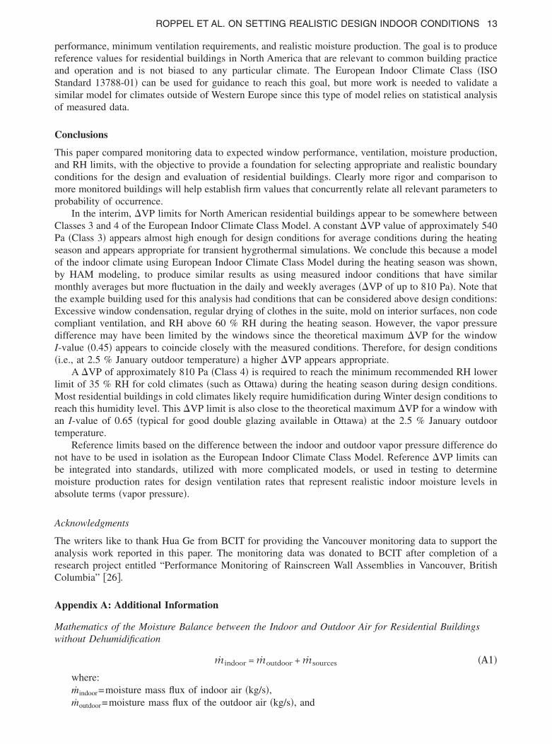
ROPPEL ET AL. ON SETTING REALISTIC DESIGN INDOOR CONDITIONS 13
performance, minimum ventilation requirements, and realistic moisture production. The goal is to producereference values for residential buildings in North America that are relevant to common building practiceand operation and is not biased to any particular climate. The European Indoor Climate Class �ISOStandard 13788-01� can be used for guidance to reach this goal, but more work is needed to validate asimilar model for climates outside of Western Europe since this type of model relies on statistical analysisof measured data.
Conclusions
This paper compared monitoring data to expected window performance, ventilation, moisture production,and RH limits, with the objective to provide a foundation for selecting appropriate and realistic boundaryconditions for the design and evaluation of residential buildings. Clearly more rigor and comparison tomore monitored buildings will help establish firm values that concurrently relate all relevant parameters toprobability of occurrence.
In the interim, �VP limits for North American residential buildings appear to be somewhere betweenClasses 3 and 4 of the European Indoor Climate Class Model. A constant �VP value of approximately 540Pa �Class 3� appears almost high enough for design conditions for average conditions during the heatingseason and appears appropriate for transient hygrothermal simulations. We conclude this because a modelof the indoor climate using European Indoor Climate Class Model during the heating season was shown,by HAM modeling, to produce similar results as using measured indoor conditions that have similarmonthly averages but more fluctuation in the daily and weekly averages ��VP of up to 810 Pa�. Note thatthe example building used for this analysis had conditions that can be considered above design conditions:Excessive window condensation, regular drying of clothes in the suite, mold on interior surfaces, non codecompliant ventilation, and RH above 60 % RH during the heating season. However, the vapor pressuredifference may have been limited by the windows since the theoretical maximum �VP for the windowI-value �0.45� appears to coincide closely with the measured conditions. Therefore, for design conditions�i.e., at 2.5 % January outdoor temperature� a higher �VP appears appropriate.
A �VP of approximately 810 Pa �Class 4� is required to reach the minimum recommended RH lowerlimit of 35 % RH for cold climates �such as Ottawa� during the heating season during design conditions.Most residential buildings in cold climates likely require humidification during Winter design conditions toreach this humidity level. This �VP limit is also close to the theoretical maximum �VP for a window withan I-value of 0.65 �typical for good double glazing available in Ottawa� at the 2.5 % January outdoortemperature.
Reference limits based on the difference between the indoor and outdoor vapor pressure difference donot have to be used in isolation as the European Indoor Climate Class Model. Reference �VP limits canbe integrated into standards, utilized with more complicated models, or used in testing to determinemoisture production rates for design ventilation rates that represent realistic indoor moisture levels inabsolute terms �vapor pressure�.
Acknowledgments
The writers like to thank Hua Ge from BCIT for providing the Vancouver monitoring data to support theanalysis work reported in this paper. The monitoring data was donated to BCIT after completion of aresearch project entitled “Performance Monitoring of Rainscreen Wall Assemblies in Vancouver, BritishColumbia” �26�.
Appendix A: Additional Information
Mathematics of the Moisture Balance between the Indoor and Outdoor Air for Residential Buildingswithout Dehumidification
mindoor = moutdoor + msources �A1�
where:mindoor=moisture mass flux of indoor air �kg/s�,˙
moutdoor=moisture mass flux of the outdoor air �kg/s�, and
14 JOURNAL OF ASTM INTERNATIONAL
msource= indoor moisture production �kg/s�.Separate moisture flux into the moisture content of air and ventilation
windoorQventilation = woutdoorQventilation + msources �A2�
where:windoor= indoor moisture content of air �kg /m3�,woutdoor=outdoor moisture content of air �kg /m3�, andQventilation=ventilation rate �m3 /s�.Use ideal gas law to convert units, PwV=wRwT,
�Po − Pi� � Qventilation
RwT= msources �A3�
where:w=mass of water vapor �g�,T=absolute temperature �K�,V=volume �m3�, andRw=0.4615 J /g·K.Rearrange terms
�VP = RwTmsources
Qventilation�A4�
Temperature Index
I =Tsurface − Toutside
Tinside − Toutside� 100 �A5�
where:I=temperature index ���,Tsurface=coldest temperature of the inside surface of a window,Toutside=outdoor temperature, andTinside= indoor temperature.
BRE Model and Adjusted Parameters
The BRE Admittance Model, presented using consistent nomenclature, is as follows �3,4,8�:
dWi
dt=
Qsource
�v− I�Wi − Wo� − ��Wi − �Wsat� �A6�
where:Wi=indoor air moisture content, kg/kg �lb/lb�,Wo=outdoor air moisture content, kg/kg �lb/lb�,Wsat=saturation moisture content of indoor air, kg/kg �lb/lb�,Qsource=moisture generation rate, kg/h �lb/h�,I=air exchange rate �ACH�,�=density of air, 1.22 kg /m3 �0.075 lb / ft3�,v=volume of space, m3 �ft3�, and� ,�=moisture admittance factors �h−1�.For steady-state conditions this formulae reduces to the following �5�:
Pi =I
I + �Po +
QsourcePtotal
0.622�v�I + ��+
�Psat
I + ��A7�
where:Pi=indoor air vapor pressure, Pa �in. Hg�,Po=outdoor air vapor pressure, Pa �in. Hg�,
Psat=saturation vapor pressure of indoor air, Pa �in. Hg�, and
ROPPEL ET AL. ON SETTING REALISTIC DESIGN INDOOR CONDITIONS 15
Ptotal= total atmosphere pressure, Pa �in. Hg�.Note that this steady-state equation equals the 160P approach equation when � and � are set to zero.
Moisture Storage of Indoor Hygroscopic Materials—Research on the moisture storage of indoorhygroscopic materials shows that the fluctuations in indoor humidity are greatly reduced by the buildingenvelope and indoor furnishings. Estimates of up to 1/3 of the water vapor generated in a room can beabsorbed by its surfaces �1�. Accordingly the exchange of moisture from the building envelope and indoorfurnishings with the indoor air becomes increasingly significant as the ventilation rate becomes low, i.e.,0.5 ACH or less �3�.
Jones �4� states that the BRE Admittance Model assumes that the whole mass of the materials isinvolved in the moisture exchanges, so there is an inherently large moisture storage capacity compared tothe amount of moisture that is exchanged with the indoor air. Jones assumes that the whole buildingmaterials come into equilibrium in weeks to months and only the surface layer several millimetres deepresponds to daily cycles. Consequently the BRE Admittance Model assumes that the moisture content ofthe indoor materials reaches an equilibrium with the indoor air over a time period where the indoorconditions remain fairly constant �ventilation and moisture generation rates�. A significant change in theequilibrium moisture content of the surface of the building materials and furnishings may occur fordifferent seasons and therefore may require different admittance factors. However, the increased ventila-tion due to occupants opening their windows during Summer and shoulder seasons for a mild marineclimate such as Vancouver is likely to have more significance. Jones �4� predicts that six pairs of admit-
TABLE 5—Summary of parameters utilized in the BRE Model for Figs. 5 and 6.
Toronto �Fig. 5� Vancouver–Building 3 �Fig. 6�
Temperature set point 15°C 11°CHeating season RHavg=22 % RHavg=57 %
�=0.6 �=0.6�=0.6�RHavg=0.132 �=0.6�RHavg=0.342
Non-heating season RHavg=39 % RHavg=38 %�=0.6 �=0.6
�=0.6�RHavg=0.234 �=0.6�RHavg=0.228
Wood Top Plate (38 mm x 89 mm)
Gypsum Board (13 mm)
Vapour Barrier
Fibreglass Insulation (89 mm)
Rigid Insulation (25 mm)
Vinyl Siding
Air Leakage
Wood Bottom Plate (38 mm x 89 mm)
2
FIG. 12—Model of wall assembly with 38�89 mm �2�4� studs.
16 JOURNAL OF ASTM INTERNATIONAL
tance factors may be sufficient to model vapor conditions for categories of high, medium, and lowmoisture admittance under Summer and Winter conditions and proposes typical values for admittancefactors for wood-lined rooms of �=0.6 and �=0.4 �3�.
The admittance terms in the BRE Admittance Model should be considered empirical to sufficientlycapture dampening effects when applied to real buildings, and it is important to look at both the dampeningterms together when selecting the admittance parameters. The first term � ·Wi �see Eq A6� calculates therate at which indoor humidity is absorbed into the building materials and furnishings and is balanced bythe second term � ·Wsat that is essentially the rate at which moisture desorbs from the surface of thebuilding materials and furnishings. If the term � ·Wi is greater than � ·Wsat, then the BRE AdmittanceModel calculates absorption of moisture into the building materials, and if the term � ·Wi is less than� ·Wsat, then the model calculates desorption of moisture from the materials to the indoor air.
The term � ·Wsat is an approximation derived from a more theoretical form of the BRE AdmittanceModel and is based on the moisture content at the surface of materials where the surface temperature isassumed to equal the temperature of the indoor air �3�. For this approximation the parameter � is equiva-lent to � ·RHs, where RHs is the RH at the surface of the building materials and furnishings. Jones �3�found that the RH at the surface of the building materials during the course of experiments ranged from 50to 70 %. Jones showed through experiments that the vapor pressure changed significantly with temperaturebut the surface RH changed by less than 10 % over a period of 1 day. An approximation for the depen-dency of the vapor pressure on temperature is incorporated into the � ·Wsat term.
The practical implication of the BRE Admittance Model is that the selection of � or � alone has onlya small impact on the calculated indoor vapor pressure and the relative difference between the � and � �orRHs� has a large impact. Since the admittance terms are dependent on the indoor vapor pressure, which isdependent on the outdoor vapor pressure, the calculated net hourly moisture mass flux from absorption/desorption is relatively independent of the selection of the admittance parameters. The effect is that achange in � relative to � will shift the calculated hourly indoor vapor pressure curve similar to a changein the assumed moisture generation rate. The same effect occurs for a change in the assumed indoor airtemperature. Essentially changes in the parameter � relative to � or the assumed air temperature changesthe assumed equilibrium air moisture content that balances whether absorption or desorption will occur.
Adjusted Parameters—The heating and non-heating � and � were selected separately to produce thecalculated �VP using the BRE Model in Figs. 5 and 6. We adjusted the parameters between the heating ornon-heating parameters based on the daily outdoor temperature. The heating parameters are used in theBRE model when temperature is below the set point and the non-heating parameters are used when thedaily temperature is above the set point. The set point was selected on a single value that visually best fitthe data. We kept � constant at 0.6 and selected � based on the mean measured indoor humidity for theappropriate season using the summarized data �Appendix B�. Table 5 summarizes our selected parameters.
This approach will slightly overestimate the �VP for a period during the shoulder seasons. Wespeculate that a robust empirical version of the BRE Model could be developed for use in a standardframework by creating a function for � dependent on the outdoor temperature and �VP limit. In ouropinion this will require analysis of many monitored buildings, over several years, to determine the bestshape of the function and best deflection points �daily, weekly, or monthly mean temperatures�. A studythat records window use, as well as the indoor and outdoor conditions, will be helpful in this pursuit.
Model Wall Assembly for Figs. 9 and 10
The wall assembly used in the simulations is based on wall assemblies that had been used previously foranalysis of condensation from air leakage �28–30�. It is a cross-section of a wood stud wall with extrudedpolystyrene insulating sheathing, fiberglass insulation in the stud cavity, and a 60 ng / �Pa·s ·m2� �1 perm�vapor barrier and painted gypsum wallboard on the interior surface. Wood stud top and bottom plates areincluded in the 2-D wall assembly as illustrated in Fig. 12.

ROPPEL ET AL. ON SETTING REALISTIC DESIGN INDOOR CONDITIONS 17
Appendix B: Monitoring Data and Analysis
TABLE 6�a�—Description of monitored Buildings 1, 2, and 3a.
Building
1 2 3aSuite location Suite 206 �south� Suite 401 �southeast� Suite 311 �east�Location Vancouver Vancouver Vancouver
TypeFour storey multi-unitresidential
Four storey multi-unitresidential
Six storey multi-unitresidential
Year Built 2000Built 1987, rehabilitated wallsand roof in 2000
Built 1990, rehabilitatedwalls in 2001
Glazing 2000 vinyl double glazed windows2001 aluminum double glazedthermally broken windows
2001 aluminum doubleglazed thermallybroken windows
Wall type2�6 wood frame with batt,rainscreen stucco
2�6 wood frame with batt,rainscreen stucco
Concrete frame withsteel stud infill and batt,exterior semi-rigidmineralfibre, stucco
Air barrier 6 mil poly new SBPO housewrap+existing poly SBS sheathing membraneInterior vaporcontrol
6 mil poly 4 mil poly Latex paint
Number ofbedrooms
2 1 2
Floor area �m2� 80 64 63Occupants 3 occupants 1 occupant 3 occupants
Exhaust and airleakage characteristics
NLA50=9.9 in.2 /100 ft2 @50 Pa exterior walls+roof, 81 %through envelope
44 CFM exhaust fancapacity on timer�approximately 6 h/day�,NLA50=3.6 in2 /100 ft2
@ 50 Pa, 33 % throughenvelope
TABLE 6�b�—Description of monitored Buildings 3a and 4.
Building
3b 4a 4b
Suite location Suite 611 �east� Suite 303 �south� Suite 309 �north�
Location Vancouver Vancouver Vancouver
TypeSix storey multi-unitresidential
Four storey multi-unitresidential
Four storey multi-unitresidential
YearBuilt 1990,rehabilitated walls in 2001
Built 2001 Built 2001
Glazing2001 aluminum doubleglazed thermallybroken windows
2001 aluminum double glazedthermally broken windows
2001 aluminumdouble glazedthermally broken windows
Wall typeconcrete frame with steelstud infill and batt, exteriorsemi-rigid mineral fibre, stucco
2�4 wood framewith batt,cement board and stucco
2�4 wood framewith batt,cement board and stucco
Air barrier SBS sheathing membrane 6 mil poly 6 mil poly
Interior vapor control Latex paint 6 mil poly 6 mil poly
Number of bedrooms 2 Bachelor suite Bachelor suite
Floor area �m2� 63 24 24
Occupants 2 occupants home regularly 1 occupant 1 occupant
Exhaust and airleakage characteristics
50 CFM exhaust fan,occupant control,not used �noise�, NLA50=6.0 in2 /100 ft2 @50 Pa, 36 % through envelope
NLA50=31.3 in2 /100 ft2
@ 50 Pa, 35 % throughenvelope

SL
T
Y
G
W
AINFOEl
A
9p
1p
18 JOURNAL OF ASTM INTERNATIONAL
TABLE 6�c�—Description of monitored Buildings 5 and 6.
Building
5a 5b 6a, 6buite location Suite 504 �south� Suite 3005 �south� Suite 205, Suite 304ocation Vancouver Vancouver Toronto
ype 30 storey multi-unit residential 30 storey multi-unit residential15 storey multi-unitresidential
ear Built 2002 Built 2002 Rehabilitated 1997
lazing 2002 aluminum double glazed windows2002 aluminum double glazed,window-wall
all typeConcrete frame with steel stud infill, stuccowall with 50 mm exterior EXPS insulation
Window wall glazingEIFS installed overmasonry
ir barrier SBS sheathing membrane N/A EIFS membranenterior vapor control Latex paint N/Aumber of bedrooms 2 2loor area �m2� 50 50ccupants Two occupants Two occupantsxhaust and air
eakage characteristics
TABLE 7�a�—Summary of monitoring data, indoor temperature �°C�.
Building/Suite Identifier
1 2 3a 3b 4a 4a 5a 5b 6a 6bverages January 23.7 18.1 16.2 17.2 23.5 22.7 23.8 20.4 23.4 22.1
February 24.0 18.9 16.6 18.8 24.0 24.4 24.1 20.2 22.4March 23.9 19.6 17.2 18.9 24.6 24.2 24.0 21.8 22.9April 24.1 21.7 14.5 14.9 23.8 24.8 22.3 24.6May 24.8 23.4 14.3 13.5 24.8 23.7 24.6 23.5 24.9June 25.6 25.3 16.7 14.4 25.9 26.1 25.2 24.5 25.7 25.0July 26.5 27.2 17.2 15.4 27.9 27.3 25.2 24.5 27.5 26.2August 26.5 26.1 15.9 16.2 27.7 26.3 24.8 24.2 27.7 25.9September 25.7 26.0 16.0 15.2 26.4 25.0 9.4 9.0 25.5 23.4October 24.4 21.3 14.8 13.8 24.7 24.4 23.2 20.5 25.5 23.4November 24.2 18.4 21.0 21.1 22.7 23.8 11.8 9.9 23.7 24.2December 23.6 18.2 18.1 18.9 22.5 23.3 11.8 10.4 23.5 23.3Jan. 1–Mar. 31 23.9 18.9 16.7 18.3 24.0 23.8 24.0 20.8 22.9April 1–Oct. 31 25.4 24.4 15.6 14.8 25.2 22.5 21.2 25.9Nov. 1–Dec. 31 23.9 18.3 19.6 20.0 22.6 23.5 11.8 10.1 23.6 23.8
0thercentiles January 25.6 20.4 17.5 18.9 25.2 25.2 25.2 22.1 24.1 23.7
February 25.8 21.5 17.5 20.2 25.3 26.1 25.4 22.1 23.9March 25.7 22.5 18.9 20.2 26.8 26.6 25.8 24.0 24.9April 26.3 24.9 20.6 20.6 25.7 26.5 25.2 25.8May 26.7 26.3 22.9 22.1 26.4 26.0 26.0 26.0 26.3June 28.0 29.4 26.9 24.1 29.1 28.3 26.7 27.6 29.3 27.7July 29.5 31.9 28.3 25.6 31.1 29.1 26.6 27.3 28.8 28.1August 29.4 29.4 27.5 26.0 30.7 27.9 27.1 27.9 28.4 27.0September 28.7 29.3 26.0 26.0 28.8 26.7 24.2 24.4 26.6 25.4October 27.0 24.4 26.7 25.0 28.0 26.7 24.4 24.4 26.6 27.7November 25.9 21.1 25.6 24.7 24.8 26.2 24.0 20.6 25.5 25.2December 24.9 21.3 21.0 20.9 24.4 25.9 24.4 21.9 24.8 25.2
0thercentiles January 22.1 16.0 14.5 15.2 22.1 16.0 22.2 18.7 21.8 20.6
February 22.5 17.0 15.2 17.5 22.5 22.5 22.6 18.6 20.4March 22.1 17.3 15.6 17.5 22.6 22.1 21.6 18.9 20.7April 22.1 18.7 22.1 23.1 19.0 22.9May 23.2 20.6 23.2 21.0 23.2 20.0 23.4June 23.6 21.3 23.4 23.6 23.9 21.1 21.7 22.0July 23.9 23.2 24.5 25.4 23.9 21.7 26.4 24.4August 24.0 22.8 24.7 24.8 23.2 21.1 23.6 22.1September 23.5 22.8 24.3 23.3 22.0 20.9October 22.5 18.4 21.3 22.1 22.8 21.4November 22.9 15.8 17.1 18.3 20.6 21.0 22.9 17.5December 22.5 15.9 15.6 17.0 20.6 20.6 22.4 20.9

A
9
1
ROPPEL ET AL. ON SETTING REALISTIC DESIGN INDOOR CONDITIONS 19
TABLE 7�b�—Summary of monitoring data, indoor RH (%).
Building/Suite Identifier
1 2 3a 3b 4a 4a 5a 5b 6a 6b
verages January 42.7 45.1 62.3 62.4 30.3 33.1 36.5 31.6 21.4 20.1
February 38.8 42.1 57.7 57.0 26.4 29.8 35.6 34.4 19.6
March 39.1 42.4 56.8 53.7 27.0 29.7 34.4 33.0 23.2
April 37.0 39.3 41.1 39.7 32.9 34.8 34.7 22.0
May 37.6 38.0 37.2 36.7 35.1 35.3 43.1 40.7 37.6
June 38.5 38.2 33.3 35.4 36.3 37.1 44.9 43.4 43.5 47.0
July 40.8 40.1 27.8 30.1 37.9 40.8 48.7 47.4 43.3 46.2
August 42.7 44.8 26.2 28.5 39.2 44.3 49.8 48.5 45.9 51.6
September 44.5 41.8 31.4 29.1 41.3 43.5 19.9 18.9 43.1 48.3
October 41.5 49.4 32.4 30.7 41.1 43.0 30.5 29.9 43.1 48.3
November 41.0 39.8 52.2 52.7 31.7 32.7 17.3 15.6 24.8 23.2
December 41.5 42.6 57.1 58.5 31.3 31.8 19.0 15.3 22.0 23.1
Jan. 1–Mar. 31 40.2 43.2 58.9 57.7 27.9 30.9 35.5 33.0 21.4
April 1–Oct. 31 40.4 41.7 32.8 32.9 39.6 38.8 37.6 39.8
Nov. 1–Dec. 31 41.3 41.2 54.6 55.6 31.5 32.2 18.1 15.5 23.4 23.2
0th percentiles January 48.3 52.1 70.3 68.3 37.6 41.6 43.3 40.8 29.7 31.8
February 45.4 47.1 67.0 62.2 29.5 33.9 42.9 42.7 25.2
March 45.8 48.7 70.0 58.9 33.3 35.5 41.5 41.5 35.8
April 45.2 47.9 63.4 58.2 39.6 43.9 47.8 29.3
May 45.8 48.0 58.5 57.7 42.5 41.2 51.0 53.3 46.7
June 45.8 47.3 50.1 56.4 42.4 42.2 53.3 55.1 53.1 59.9
July 48.3 47.5 46.7 51.0 45.1 45.6 55.7 57.2 53.4 60.5
August 52.6 56.4 47.4 47.9 45.7 49.1 57.4 57.1 57.8 66.0
September 52.3 48.6 53.4 50.8 48.4 47.8 54.7 52.5 56.6 61.6
October 48.1 60.6 56.9 56.1 48.6 47.5 48.7 44.6 51.5 58.2
November 49.4 47.2 63.3 64.4 40.8 38.7 39.9 37.5 29.6 30.7
December 46.9 47.8 66.0 65.0 35.8 37.1 42.4 34.8 29.3 29.0
0th percentiles January 37.5 34.5 53.1 55.6 21.7 22.0 28.4 19.3 15.1 11.6
February 31.9 35.6 47.4 51.5 22.5 24.4 28.7 26.4 14.8
March 32.2 36.1 43.8 47.9 21.5 23.0 27.6 24.8 13.7
April 27.5 30.2 27.0 27.2 24.7 15.2
May 30.2 30.5 28.9 29.9 34.7 30.0 26.5
June 30.4 30.3 30.2 32.3 37.0 32.0 26.5 26.6
July 33.5 32.9 31.5 35.5 42.2 39.0 33.2 33.5
August 33.6 34.8 32.8 39.5 42.2 40.4 35.8 38.7
September 36.3 34.2 33.6 38.7 33.9 32.7
October 33.8 39.4 30.9 36.6 21.3 16.1
November 32.8 32.7 41.3 42.8 22.2 25.6 15.9 16.2
December 36.3 36.6 48.5 51.2 25.8 27.1 17.3 13.4

A
9
1
20 JOURNAL OF ASTM INTERNATIONAL
TABLE 7�c�—Summary of monitoring data, indoor vapor pressure (Pa).
Building/Suite Identifier
1 2 3a 3b 4a 4a 5a 5b 6a 6b
verages January 1251.8 944.6 1151.4 1222.7 881.8 911.9 1085.0 762.9 611.8 545.1
February 1155.1 921.3 1090.2 1240.6 786.3 914.2 1078.3 813.4 535.7
March 1154.6 966.9 1121.4 1171.3 831.2 902.6 1036.7 852.6 665.1
April 1104.4 1013.3 1139.7 1144.6 970.0 1093.3 924.0 679.9
May 1172.3 1087.5 1197.4 1092.6 1102.1 1048.1 1335.5 1160.7 1197.0
June 1252.9 1218.2 1054.0 907.0 1214.8 1253.7 1443.1 1322.6 1484.8 1535.1
July 1404.0 1443.4 963.3 857.6 1428.5 1484.6 1559.8 1446.7 1599.3 1575.5
August 1469.0 1496.0 892.7 871.3 1454.0 1515.3 1563.3 1461.9 1706.8 1734.4
September 1461.9 1394.0 931.4 864.1 1420.9 1381.2 1457.6 1300.6 1421.3 1405.1
October 1271.0 1264.9 878.1 812.9 1291.1 1317.0 899.9 745.7 1421.3 1405.1
November 1229.9 840.7 1295.0 1306.8 868.2 970.7 972.9 695.9 728.9 702.6
December 1211.8 895.5 1197.5 1282.2 852.1 914.9 1103.7 745.4 646.8 663.9
Jan. 1–Mar. 31 1187.2 944.3 1121.0 1211.6 833.1 909.5 1066.6 809.6 604.2
April 1–Oct. 31 1305.1 1273.9 1008.1 935.7 1281.4 1336.1 1194.6 1358.6
Nov. 1–Dec. 31 1220.8 868.1 1246.2 1294.5 860.1 942.8 1038.3 720.7 687.8 683.3
0th percentiles January 1398.3 1117.1 1329.2 1373.6 1130.5 1156.5 1349.4 990.8 887.6 907.6
February 1319.8 1052.1 1229.9 1368.5 895.0 1062.4 1348.0 998.1 711.6
March 1328.7 1118.6 1438.3 1313.0 984.1 1106.6 1328.1 1025.1 1130.8
April 1308.6 1215.8 1299.9 1282.1 1178.1 1417.7 1163.9 884.1
May 1399.2 1272.8 1505.4 1301.3 1381.8 1304.9 1596.8 1356.2 1525.3
June 1439.0 1424.1 1569.7 1320.0 1411.9 1455.1 1742.6 1632.1 1981.6 2055.1
July 1611.4 1681.5 1638.5 1533.3 1692.3 1738.4 1753.6 1649.5 2015.3 2136.8
August 1687.9 1702.2 1621.9 1495.2 1677.4 1728.8 1823.3 1721.4 2193.0 2218.5
September 1685.8 1591.8 1553.9 1528.4 1677.1 1563.9 1680.5 1448.7 1888.9 1878.0
October 1489.1 1573.3 1520.2 1441.3 1656.2 1528.8 1633.0 1448.2 1741.3 1802.7
November 1462.8 993.8 1538.0 1463.7 1098.3 1235.5 1243.2 927.7 913.4 865.1
December 1355.4 1046.6 1534.6 1519.9 975.3 1144.1 1350.2 897.9 879.5 764.9
0th percentiles January 1116.0 684.9 938.3 1060.2 616.3 627.9 767.4 457.3 411.9 284.0
February 975.1 811.2 927.5 1097.6 672.2 745.7 809.5 653.9 382.8
March 996.6 831.6 832.3 999.5 683.9 637.4 788.9 676.6 361.8
April 871.4 841.8 950.1 997.3 795.1 834.7 708.0 473.6
May 967.5 891.5 911.3 909.0 905.9 778.8 1060.5 960.0 788.6
June 1077.9 1025.2 997.6 1054.1 1172.8 1043.0 729.1 702.0
July 1188.0 1191.5 1151.3 1227.1 1370.4 1230.8 1171.8 1097.5
August 1253.3 1313.8 1254.2 1319.7 1303.2 1210.2 1272.6 1197.7
September 1229.0 1239.2 1174.6 1189.5 1246.1 1082.9 1032.6 876.9
October 1074.7 862.1 958.2 1115.2 556.7 405.0 612.6 553.1
November 1029.1 654.7 995.7 1147.8 624.2 716.2 684.2 444.7 483.1 403.6
December 1078.5 748.9 905.0 1060.0 725.1 716.4 852.7 584.3 486.2 344.9

A
9p
1p
ROPPEL ET AL. ON SETTING REALISTIC DESIGN INDOOR CONDITIONS 21
TABLE 7�d�—Summary of monitoring data, vapor pressure difference (�VP, Pa).
Building/Suite Identifier
1 2 3a 3b 4a 4a 5a 5b 6a 6b
verages January 456.5 128.1 331.2 402.6 98.4 151.7 298.2 �24.0 166.1 83.1
February 408.2 147.6 316.4 466.8 �13.7 164.9 303.2 38.3 86.1
March 368.6 108.1 338.8 388.7 �26.2 124.1 180.9 �3.2 74.7
April 199.9 81.4 195.1 198.9 82.3 152.6 �16.7 51.1
May 107.9 �43.0 119.2 40.4 �90.7 �33.5 205.4 30.6 �81.0
June �25.3 �111.1 86.3 �60.6 �78.0 �50.1 108.1 �12.4 �102.1 �67.8
July �78.1 �111.5 30.3 �116.0 �74.0 �21.6 4.4 �108.7 �66.3 �90.1
August �49.0 �58.1 39.4 �86.4 �44.1 17.8 4.9 �96.5 �56.0 �28.3
September 14.9 �8.8 26.3 4.1 62.6 22.9 102.1 �90.6 28.7 16.0
October 108.0 36.0 140.2 135.6 79.6 84.7 175.7 12.2 28.7 16.0
November 362.0 65.4 300.5 308.4 24.1 178.2 264.2 �12.7 88.5 62.2
December 463.3 76.6 280.2 336.7 74.7 151.5 359.0 0.7 54.7 71.2
Jan. 1–Mar. 31 411.1 127.9 328.8 419.4 19.5 146.9 260.7 3.7 109.0
April 1–Oct. 31 39.8 �30.7 91.0 16.6 14.6 107.6 �40.3 �28.1
Nov. 1–Dec. 31 412.6 71.0 290.4 322.5 49.4 164.8 311.6 �6.0 71.6 66.7
0thercentiles January 720.4 319.8 519.1 617.0 296.5 373.8 683.5 111.4 315.5 206.4
February 611.0 285.4 513.2 626.6 121.3 396.1 666.6 316.1 235.2
March 588.8 272.4 582.5 571.7 119.9 320.9 500.2 183.9 237.1
April 470.2 295.1 408.0 452.6 288.8 518.3 252.1 233.4
May 329.9 116.6 395.0 317.6 118.7 221.2 615.2 387.5 149.2
June 203.8 41.6 285.0 104.1 143.6 168.3 492.9 348.1 89.3 97.7
July 112.7 56.2 193.7 58.7 228.3 236.1 322.6 176.9 217.8 76.0
August 143.6 72.4 202.8 91.5 145.9 230.8 276.1 144.7 221.5 130.0
September 204.8 0.0 182.1 164.4 320.7 204.8 343.1 100.9 259.2 170.5
October 357.5 179.2 462.1 473.0 334.8 303.1 394.9 102.4 245.4 157.6
November 587.9 240.0 859.4 759.0 204.1 395.9 581.5 78.0 256.6 151.5
December 658.8 251.9 725.6 702.9 223.4 404.4 654.0 83.4 352.9 179.6
0thercentiles January 235.4 �51.3 151.7 210.0 �49.8 �74.6 �42.9 �193.0 13.2 �47.2
February 206.9 11.5 118.4 303.7 �123.5 �15.7 �11.5 �140.0 �32.4
March 169.6 �47.5 121.9 213.6 �157.0 �67.0 �103.0 �173.3 �94.4
April �100.5 �113.1 0.0 0.0 �146.5 �147.8 �245.8 �103.0
May �127.0 �186.4 �12.1 �168.5 �262.9 �265.0 �130.2 �222.4 �309.4
June �290.5 �315.7 �60.7 �296.8 �332.2 �305.1 �219.4 �307.2 �291.0 �251.7
July �285.2 �277.6 �91.7 �451.1 �330.7 �275.5 �283.5 �384.7 �287.8 �250.3
August �249.5 �196.5 �64.7 �401.1 �239.6 �196.1 �287.2 �384.4 �262.4 �173.5
September �184.2 �65.4 �107.3 �152.9 �171.7 �158.9 �94.7 �326.9 �182.7 �157.3
October �123.9 �34.5 �6.6 �7.1 �153.5 �125.6 �78.7 �122.7 �155.4 �146.4
November 149.5 0.0 0.0 0.0 �131.8 �30.9 �2.7 �102.4 �78.6 �85.7
December 276.4 0.0 0.0 0.0 �80.6 �42.6 67.8 �72.8 �33.0 �58.7

22 JOURNAL OF ASTM INTERNATIONAL
7�e�
—Su
mm
ary
ofm
onit
orin
gda
ta,
indo
orde
wpo
int
tem
pera
ture
�°C
�.
Bui
ldin
g/Su
iteId
entifi
er
3a3b
4a4a
5a5b
6a6b
98.
99.
94.
85.
37.
82.
4�
0.6
�2.
77
8.2
10.1
3.4
5.6
7.9
3.8
�2.
34
8.4
9.3
4.2
5.2
7.3
4.5
0.1
18.
88.
96.
48.
05.
61.
01
9.2
7.9
10.3
7.4
11.1
9.1
9.2
812
.09.
79.
710
.212
.311
.012
.112
.54
12.8
10.6
12.3
12.8
13.6
12.4
13.8
13.4
912
.710
.911
.813
.113
.612
.514
.814
.89
11.9
11.4
12.1
11.7
12.4
10.6
11.9
111
.110
.810
.411
.04.
41.
111
.93
10.7
10.9
4.7
6.3
6.3
1.4
2.2
1.7
39.
410
.54.
65.
58.
22.
60.
10.
40
8.5
9.8
4.1
5.3
7.7
3.6
�0.
93
11.2
10.0
10.4
10.8
8.9
10.7
810
.010
.74.
65.
97.
22.
01.
21.
0
611
.211
.78.
89.
111
.46.
95.
35.
67
10.1
11.7
5.4
7.9
11.4
7.0
2.1
612
.411
.06.
88.
511
.27.
48.
89
10.9
10.7
9.4
12.2
9.2
5.2
613
.110
.913
.310
.914
.011
.513
.33
14.0
11.4
12.2
12.6
15.4
14.3
17.4
17.9
814
.713
.715
.415
.315
.514
.517
.618
.60
14.7
13.4
13.9
15.2
16.1
15.2
19.0
19.2
013
.913
.714
.813
.714
.812
.116
.68
13.5
12.8
14.6
13.3
13.8
11.7
15.3
913
.412
.78.
410
.110
.25.
95.
74.
97
13.4
13.3
6.6
9.0
11.5
5.4
5.1
3.1
66.
17.
90.
10.
43.
1�
4.0
�5.
4�
10.4
05.
98.
41.
32.
83.
90.
9�
6.4
34.
37.
01.
50.
63.
61.
4�
7.2
56.
37.
03.
74.
42.
0�
3.5
35.
65.
67.
33.
47.
96.
43.
64
10.1
7.9
6.5
7.8
9.3
7.6
2.4
1.9
610
.67.
88.
510
.011
.710
.19.
38.
40
10.6
8.5
9.8
11.1
10.9
9.8
10.6
9.7
29.
79.
19.
49.
610
.18.
07.
58
8.2
8.4
6.4
8.6
�3.
3�
7.7
0.0
96.
99.
00.
32.
21.
6�
4.4
�3.
3�
5.7
85.
57.
92.
42.
24.
7�
0.7
�3.
2�
7.8
TAB
LE
Dew
Poin
t�°
C�
12
Ave
rage
sJa
nuar
y10
.35.
Febr
uary
9.0
5.M
arch
9.0
6.A
pril
8.3
7.M
ay9.
28.
June
10.2
9.Ju
ly12
.012
.A
ugus
t12
.612
.Se
ptem
ber
12.6
11.
Oct
ober
10.4
10.
Nov
embe
r9.
94.
Dec
embe
r9.
85.
Jan.
1–M
ar.
319.
46.
Apr
il1–
Oct
.31
10.8
10.
Nov
.1–
Dec
.31
9.9
4.
90th
perc
entil
esJa
nuar
y12
.08.
Febr
uary
11.1
7.M
arch
11.2
8.A
pril
11.0
9.M
ay12
.010
.Ju
ne12
.412
.Ju
ly14
.214
.A
ugus
t14
.915
.Se
ptem
ber
14.8
14.
Oct
ober
12.9
13.
Nov
embe
r12
.76.
Dec
embe
r11
.57.
10th
perc
entil
esJa
nuar
y8.
61.
Febr
uary
6.6
4.M
arch
6.9
4.A
pril
5.0
4.M
ay6.
55.
June
8.1
7.Ju
ly9.
59.
Aug
ust
10.3
11.
Sept
embe
r10
.010
.O
ctob
er8.
14.
Nov
embe
r7.
40.
Dec
embe
r8.
12.

ROPPEL ET AL. ON SETTING REALISTIC DESIGN INDOOR CONDITIONS 23
FIG. 13—Vancouver, Building 1: Vapor pressure difference (�VP, Pa).
FIG. 14—Vancouver, Building 1: Indoor vapor pressure (Pa) and RH (%).
FIG. 15—Vancouver, Building 1: Indoor and outdoor temperatures �°C�.

24 JOURNAL OF ASTM INTERNATIONAL
FIG. 16—Vancouver, Building 2: Vapor pressure difference (�VP, Pa).
FIG. 17—Vancouver, Building 2: Indoor vapor pressure (Pa) and RH (%).
FIG. 18—Vancouver, Building 2: Indoor and outdoor temperatures �°C�.

ROPPEL ET AL. ON SETTING REALISTIC DESIGN INDOOR CONDITIONS 25
FIG. 19—Vancouver, Building 3: Vapor pressure difference (�VP, Pa).
FIG. 20—Vancouver, Building 3: Indoor vapor pressure (Pa).
FIG. 21—Vancouver, Building 3: Indoor RH (%).

26 JOURNAL OF ASTM INTERNATIONAL
FIG. 22—Vancouver, Building 3: Indoor and outdoor temperatures �°C�.
FIG. 23—Vancouver, Building 4: Vapor pressure difference (�VP, Pa).
FIG. 24—Vancouver, Building 4: Indoor vapor pressure (Pa).

ROPPEL ET AL. ON SETTING REALISTIC DESIGN INDOOR CONDITIONS 27
FIG. 25—Vancouver, Building 4: Indoor RH (%).
FIG. 26—Vancouver, Building 4: Indoor and outdoor temperatures �°C�.
FIG. 27—Vancouver, Building 5: Vapor pressure difference (�VP, Pa).

28 JOURNAL OF ASTM INTERNATIONAL
FIG. 28—Vancouver, Building 5: Indoor vapor pressure (Pa).
FIG. 29—Vancouver, Building 5: Indoor RH (%).
FIG. 30—Vancouver, Building 5: Indoor and outdoor temperatures �°C�.

ROPPEL ET AL. ON SETTING REALISTIC DESIGN INDOOR CONDITIONS 29
FIG. 31—Toronto, Building 6: Vapor pressure difference (�VP, Pa).
FIG. 32—Toronto, Building 6: Indoor vapor pressure (Pa).
FIG. 33—Toronto, Building 6: Indoor RH (%).

30 JOURNAL OF ASTM INTERNATIONAL
References
�1� Kusuda, T., “Indoor Humidity Calculation,” ASHRAE Trans., Vol. 89, No. 2, 1983, pp. 728–738.�2� International Energy Agency, “Condensation and Energy: Source Book,” Report Annex 14, Vol. 1,
KU Leuven, Belgium, 1991, http://www.ecbcs.org/annexes/annex14.htm. �Last accessed date July29, 2009�.
�3� Jones, R., “Modelling Water Vapour Conditions in Buildings,” Build. Services Eng. Res. Technol.,Vol. 14, No. 3, 1993, pp. 99–106, Building Research Establishment, Watford, UK.
�4� Jones, R., “Indoor Humidity Calculation Procedure,” Build. Services Eng. Res. Technol., Vol. 16, No.3, 1995, pp. 119–126, Building Research Establishment, Watford, UK.
�5� Djebbar, R., van Reenen, D., and Kumaran, M. K., “Indoor and Outdoor Weather Analysis Tool forHygrothermal Modelling”, 8th Conference of Building Science and Technology, Toronto, Ontario,IRC-National Research Council Canada, Ottawa, ON, 2001, pp. 139–157.
�6� TenWolde, A. and Walker, I. S., “Interior Moisture Design Loads for Residences,” Proceedings of theSeventh International Conference on the Performance of Whole Buildings, Clearwater, FL, 2001,ASHRAE, Atlanta, GA.
�7� BSR/ASHRAE Standard 160P-06, 2006, “Design Criteria for Moisture Control in Buildings,” Ameri-can Society of Heating, Refrigeration and Air-Conditioning Engineers, Inc., Atlanta, GA.
�8� Roppel, P., Brown, W. C., and Lawton, M., “Modeling of Uncontrolled Indoor Humidity for HAMSimulations of Residential Buildings,” Proceedings of the Tenth International Conference on thePerformance of Whole Buildings, Clearwater, FL, 2007, ASHRAE, Atlanta, GA, http://www.morrisonhershfield.com/newsroom/TechnicalPapers/Pages/default.aspx. �Last accessed dateJuly 29, 2009�.
�9� Cornick, S. and Kumaran, M. K., “A Comparison of Empirical Indoor Relative Humidity withMeasured Data,” Journal of Building Physics, Vol. 31, No. 3, January 2008, pp. 243–268, �NRCC-49235�, http://www.nrc-cnrc.gc.ca/obj/irc/doc/pubs/nrcc49235/nrcc49235.pdf. �Last accessed dateJuly 29, 2009�.
�10� Sanders, C., “Heat, Air and Moisture Transfer in Insulated Envelope Parts, Task 2: EnvironmentalConditions,” Report Annex 24, Vol. 2, KU Leuven, Belgium, 1996, http://www.ecbcs.org/annexes/annex24.htm. �Last accessed date July 29, 2009�.
�11� Kalamees, T. and Vinha, J., “Indoor Humidity Loads and Moisture Production in LightweightTimber-Frame Detached Houses,” Journal of Building Physics, Vol. 29, No. 3, January 2006, http://jen.sagepub.com/cgi/content/refs/29/3/219. �Last accessed date July 29, 2009�.
�12� Kumaran, M. K., Sanders, C. H., Tariku, F., Cornick, S., Hens, H., Blocken, B., Carmeliet, J., de
FIG. 34—Toronto, Building 6: Indoor and outdoor temperatures �°C�.
Paepe, M., and Janssens, A., “Boundary Conditions and Whole Building HAM Analysis,” Annex 41

ROPPEL ET AL. ON SETTING REALISTIC DESIGN INDOOR CONDITIONS 31
Whole Building Heat, Air, Moisture Response, Vol. 2, KU Leuven, Belgium, 2008, ISBN 978-90-334-7059-2.
�13� ISO Standard 13788-01, 2001, “Hygrothermal Performance of Building Components and BuildingElements—Internal Surface Temperature to Avoid Critical Surface Humidity and InterstitialCondensation—Calculation Methods,” International Organization for Standardization, Geneva, Swit-zerland.
�14� Hutcheon, N. B., “Humidity in Canadian Buildings,” Canadian Building Digest, National ResearchCouncil Canada, Ottawa, ON, 1960 �revised 1968�, http://www.nrc-cnrc.gc.ca/eng/ibp/irc/cbd/building-digest-1.html. �Last accessed date July 29, 2009�.
�15� Health Canada, “Exposure Guidelines for Residential Indoor Air Quality. A Report of the Federal-Provincial Advisory Committee on Environmental and Occupational Health,” Environmental HealthDirectorate, Health Protection Branch, Ottawa, ON, 1987 �revised 1989�, http://www.hc-sc.gc.ca/ewh-semt/pubs/air/exposure-exposition/index-eng.php. �Last accessed date July 29, 2009�.
�16� ASHRAE Standard 62.2-04, 2004, “Ventilation and Acceptable Indoor Air Quality in Low-RiseResidential Buildings,” American Society of Heating, Refrigeration and Air-Conditioning Engineers,Inc., Atlanta, GA.
�17� International Code Council, 2006, “2006 IECC: 2006 International Energy Conversation Code,” FallsChurch, Virginia.
�18� ANSI/ASHRAE 169-06, 2006, “Weather Data for Building Design Standards,” American Society ofHeating, Refrigeration and Air-Conditioning Engineers, Inc., Atlanta, GA.
�19� ANSI/ASHRAE/IESNA 90.1-07, 2007, “Energy Standard for Buildings except Low-Rise ResidentialBuildings,” American Society of Heating, Refrigeration and Air-Conditioning Engineers, Inc., At-lanta, GA.
�20� Chown, G. A., “Committee Paper on Application of NBC Part 9 Building Envelope DiffusionRequirements Depending on Indoor Relative Humidity,” National Research Council Canada, Ottawa,ON, 2003.
�21� CMHC, “Condensation in the Home: Where, Why, and What to Do About It,” Canada Mortgage andHousing Corporation, Ottawa, ON, 1982.
�22� Handegord, G. O., “Moisture Sources in Houses,” Building Science Insight, National Research Coun-cil Canada, Ottawa, ON, 1983.
�23� Lawton, M. D., Dales, R. E., and White, J., “The Influence of House Characteristics in a CanadianCommunity on Microbiological Contamination,” Indoor Air, Munksgaard, Copenhagen, Denmark,1998.
�24� Carll, C., TenWolde, A., and Munson, R., “Moisture Performance of a Contemporary Wood-FrameHouse Operated at Design Humidity Levels,” Proceedings of the Tenth International Conference onthe Performance of Whole Buildings, Clearwater, FL, 2007, ASHRAE, Atlanta, GA.
�25� TenWolde, A. and Pilon, C. L., “The Effect of Indoor Humidity on Water Vapor Release in Houses,”Proceedings of the Tenth International Conference on the Performance of Whole Buildings, Clear-water, FL, 2007, ASHRAE, Atlanta, GA.
�26� Finch, G., Straube, J., and Hubbs, B., “Building Envelope Performance Monitoring and Modeling ofWest Coast Rainscreen Enclosures,” Proceedings of the Third Annual International Building PhysicsConference, Montreal, QC, 2006, The Alberta Building Envelope Council �South�, Calgary, Alberta.
�27� Roppel, P., Lawton, M., and Hubbs, B., “Balancing the Control of Heat, Air, Moisture, and Compet-ing Interests,” Proceedings of the 11th Canadian Building Science and Technology Conference,Banff, AB, 2007, The Alberta Building Envelope Council �South�, Calgary, Alberta, http://www.morrisonhershfield.com/newsroom/TechnicalPapers/Pages/default.aspx. �Last accessed dateJuly 29, 2009�.
�28� Brown, C. M., Roppel, P., and Lawton, M., “Developing a Design Protocol for Low Air and VapourPermeance Insulating Sheathing in Cold Climates,” Proceedings of the Tenth International Confer-ence on the Performance of Whole Buildings, Clearwater, FL, 2007, ASHRAE, Atlanta, GA, http://www.morrisonhershfield.com/newsroom/TechnicalPapers/Pages/default.aspx. �Last accessed date
July 29, 2009�.
32 JOURNAL OF ASTM INTERNATIONAL
�29� Ojanen, T. and Kumaran, M. K., “Air Exfiltration and Moisture Accumulation in Residential WallCavities,” Proceedings of the Fifth International Conference on the Thermal Performance of ExteriorEnvelopes of Whole Buildings, Clearwater, FL, 1992, ASHRAE, Atlanta, GA, pp. 491–500.
�30� Ojanen, T. and Kumaran, M. K., “Effect of Exfiltration on the Hygrothermal Behavior of a Residen-tial Wall Assembly,” Journal of Thermal Insulation and Building Envelopes, Vol. 19, 1996,pp. 215–227.


![Indoor Relative Humidity in Residential Buildings – A Necessary Boundary …¼nzel - Indoor Relative... · 2014. 5. 20. · Maintenance and Monument Preservation (WTA) 6-2 [13]](https://img.pdfslide.us/doc/110x75/613e59aa59df642846167959/indoor-relative-humidity-in-residential-buildings-a-a-necessary-boundary-nzel.jpg)