Noname manuscript No.(will be inserted by the editor)

Setpoint Regulation forStochastically Interacting Robots

Nils Napp · Samuel Burden · Eric Klavins

the date of receipt and acceptance should be inserted later

Abstract We present an integral feedback controller

that regulates the average copy number of an assembly

in a system of stochastically interacting robots. Themathematical model for these robots is a tunable reac-

tion network, which makes this approach applicable to

a large class of other systems, including ones that ex-

hibit stochastic self-assembly at various length scales.We prove that this controller works for a range of set-

points and how to compute this range both analytically

and experimentally. Finally, we demonstrate these ideason a physical testbed.

1 Introduction

Self-assembly of complex systems and structures promisesmany new applications, such as easily combining differ-

ent micro-fabrication technologies [1] or building arbi-

trary, complex nano-structures [2]. While many naturalsystems are reliably self-assembled at vastly different

length and time scales, engineered self-assembled sys-

tems remain comparatively simple. The difficulties ofengineering complex self-assembling systems are associ-

ated with large configuration spaces, our lack of under-

Nils Napp · Eric Klavins

Electrical EngineeringUniversity of WashingtonSeattle WA 98195

Tel.: +1 206 685 8678

Fax.: +1 206 543 3842

E-mail: nnapp@uw.edu

E-mail: klavins@uw.edu

Samuel BurdenElectrical EngineeringUniversity of California at BerkeleyBerkeley CA 94720E-mail: sburden@eecs.berkeley.edu

standing the relationship between local and global dy-

namics, and the stochastic or uncertain nature of their

dynamic models.

In the context of engineering such systems, the in-terplay between uncertainty and sensitivity of global to

local behavior can often lead to a profound lack of mod-

ularity as small unintended local interactions can dras-tically alter the behavior from what is expected by com-

position. In this paper we partially address this problem

by designing a feedback controller that can regulate the

expected value of the number of an arbitrary compo-nent type. This approach could be used for composition

in the sense that other subsystems can rely on the pres-

ence of these regulated quantities.

We are guided by the application of stochastic self-

assembly, in which self-assembling particles interact ran-

domly. Such systems abound in engineered settings,

such as in DNA self-assembly [2], micro and meso-scaleself-assembly [1,3–5], and robotic self-assembly [6,7]. It

is also the prevailing model for self-assembly in biolog-

ical systems.

Self-assembly can be either passive or active. Design-ing systems that passively self-assemble is a problem of

engineering a favorable free energy landscape in con-

figuration space. Passively self-assembling systems of-ten lack flexibility since a specific energy landscape can

be difficult to adapt to new tasks. In addition, there

are physical limitations to how much the energy land-

scape can be manipulated. The yield of a desired outputstructure is a function of both the shape and depth of

energy wells. As a result of the physical limits on ma-

nipulating the energy landscape, passive self-assemblygenerally leads to low yields.

In active self-assembly, energy can be locally in-

jected into the system. In particular, we focus on the

situation where some particles have the ability to selec-

2

Natural Dynamics

Disassembly Reaction

Recharge Reaction

P1

P2

GGGGGGGGGGGA

D GGGGGGGGGGG

P12

P12A

GGGGGGGGGGGA

P1

P2

A′

A′

GGGGGGGGGGGAA

Fig. 1 Schematic representation of robot interactions. The pas-sive robots P1 and P2 can form heterodimers, which can disas-semble spontaneously. The active robot A can expend energy toundo bonds. When the arms of an active robot are retracted, it is

charged and can actively disassemble a dimer. If the arms of anactive robot are extended (denoted A′) then the it is not charged,but may become charged via the recharge reaction, the rate of

which can be controlled.

tively undo bonds that are formed by passive dynam-ics. The input of available energy is global, but how it

is used to undo bonds is decided locally by the self-

assembling particles, similar to the availability of nu-trients that power bio-chemical processes. Active self-

assembly can overcome the lack of flexibility of passively

self-assembling system by making aspects of the systemre-programmable while leaving other areas in the en-

ergy landscape untouched. As a result, the changes in

the global dynamics remain tractable.

The particular model for active self-assembly we

investigate is that of a tunable reaction network. Wepresent a system of simple stochastically interacting

robots that are well modeled as a tunable reaction net-

work and demonstrate a feedback setpoint regulationscheme. Fig. 1 shows a pictorial representation of the

tunable reaction network investigated in this paper.

There are three robot types and several instances of

each (see Fig. 2(a)). The passive robots P1 and P2

are able to bind and form heterodimer complexes P12,

which in turn can spontaneously disassemble. The ac-

tive robots A can dock with heterodimers and disassem-ble them. The disassembly reaction leaves active robots

in an uncharged state, denoted by A′. The last reac-

tion in Fig. 1 recharges uncharged robots at a rate thatis controlled externally. It corresponds to the rate at

which energy is delivered to the system globally. The

control problem for this system is to regulate the num-

ber of heterodimers P12 in the system by adjusting the

recharge rate. (This problem is re-stated formally in

Sec. 6.) While the tunable reaction network shown in

Fig. 1 is comparatively simple, tunable reaction net-

works in general can describe much more complicated

systems.

For example, many biological systems can be viewed

as tunable reaction networks. Inside cells, enzymes areexpressed to control the rates of various metabolic re-

actions. Similar to the problem solved here, one of the

many functions of the biochemical processes inside cellsis maintaining equilibria of chemical species. Regulat-

ing the concentration of chemical species is a particular

aspect of homeostasis, which can be viewed as a controlproblem [8].

For the artificial systems depicted in Fig. 1 we pro-

pose, analyze, and implement a feedback controller. Therobots serve as a physical instantiation of a tunable re-

action network. Using such a simple system also allows

us examine some of the model assumptions in some de-tail. However, the theorem and proof in Sec. 5 do not

rely on any special structure of the example network, so

that the results are applicable to many other systems,including ones with more species and intermediate as-

sembly steps.

In the context of engineering self-assembling sys-

tems, the proposed feedback controller can be used to

provide stable operating conditions for other self-ass-

embling processes, much like homeostasis in biologicalsystems. For example, in a hypothetical system with a

vat of self-assembling miniature robots, we might care

that the relative concentration of robot feet and robotlegs is fixed in order to maximize the yield of function-

ing robots. In general, we envision the self-assembling

systems of the future as having metabolisms of theirown that regulate the various species of partially as-

sembled objects in the system to maximize the yield of

the desired final assembly.

2 Experimental Robotic Chemistry

The robots described here fall in the broad class of

modular robots as there are many identical copies ofeach robot type comprising the overall system. For an

overview of this vast area of research see, for exam-

ple [9]. Specifically, the robots in this paper are stochas-tic modular robots as in [6,7,10,11], however, they are

much simpler both mechanically and electronically. Also,

while many robotic platforms consist of a homogeneousgroup of robots, the robotic testbed described here is a

heterogeneous mixture of three different robot types,

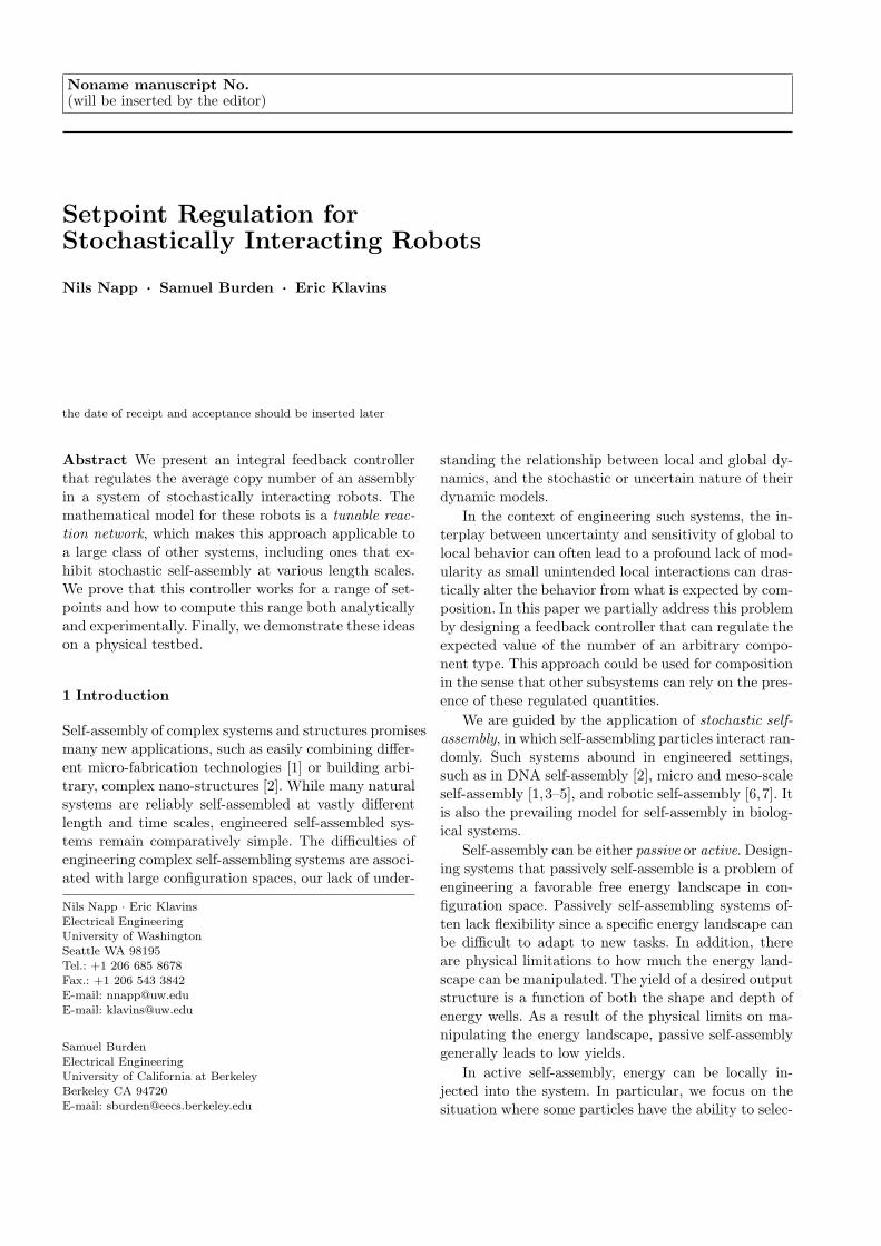
Fig. 2(b)(c). The assembly of the two passive robot

types P1 and P2 is driven by complementary shape andembedded magnets. The magnetic force creates an en-

ergy well that tends to pull P1 and P2 robots together

to form a heterodimer. The third, active robot type

3

can expend energy to disassemble a heterodimer into

its constituents.The energy for this disassembly is supplied to the

active robots via solar panels. Each active robot stores

energy from its solar panel in a capacitor, if the chargein the capacitor reaches a threshold and an active robot

A is bound to a heterodimer a motor activates and dis-

assembles it. Disassembling heterodimers depletes theon-board energy storage of active robots requiring more

energy from the solar cells to disassemble additional

heterodimers. Adjusting the amount of incident light

changes the recharge rate of active robots and thus in-directly affects the rate at which heterodimers are dis-

assembled.

Although this indirect approach may seem unneces-sarily complicated, it possesses a key design feature that

we believe justifies the added complexity: the struc-

tural, energy delivery, and computational functions re-side on separate components of the overall system. We

think of P1 and P2 as the structural components we

want to control, the active robots as agents of energy

delivery, and the controller implemented on a computeras the computational component. This division of labor

is analogous to many biological systems where differ-

ent cellular functions are largely separated into differenttypes of molecules. We believe that such a separation

of functionality in self-organization is essential to engi-

neering large scale complex systems. Distributing thefunctionality in this way can yield much simpler indi-

vidual components on average. For example, supplying

energy externally allows micro-robots to be simpler in

construction [12]. In this example, the passive robotscontain no electronic components whatsoever, and the

active robots only contain a simple circuit made from

discrete electrical components, a motor, and a solarpanel.

2.1 Physical Characteristics of Testbed

The body of each robot is machined from polyurethaneprototyping foam and painted black to aid the vision

system. This material is easy to machine, light, and

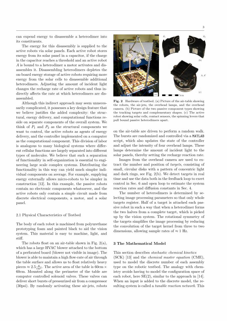
stiff.The robots float on an air-table shown in Fig. 2(a),

which has a large HVAC blower attached to the bottom

of a perforated board (blower not visible in image). Theblower is able to maintain a high flow-rate of air through

the table surface and allows us to float relatively heavy

pieces ≈ 2.5 g

cm2 . The active area of the table is 60cm×

60cm. Mounted along the perimeter of the table arecomputer controlled solenoid valves. These valves can

deliver short bursts of pressurized air from a compressor

(30psi). By randomly activating these air-jets, robots

60cm

60cm

P1 P2

A, A′

(a)

(b)

(c)

5cm

Fig. 2 Hardware of testbed. (a) Picture of the air-table showingthe robots, the air-jets, the overhead lamps, and the overheadcamera. (b) Picture of the two passive component types showingthe tracking targets and complementary shapes. (c) The active

robot showing solar cells, contact sensors, the spinning levers thatpull bound passive heterodimers apart.

on the air-table are driven to perform a random walk.The bursts are randomized and controlled via a MATLAB

script, which also updates the state of the controller

and adjust the intensity of four overhead lamps. Theselamps determine the amount of incident light to the

solar panels, thereby setting the recharge reaction rate.

Images from the overhead camera are used to ex-

tract the number and position of targets, consisting ofsmall, circular disks with a pattern of concentric light

and dark rings, see Fig. 2(b). We detect targets in real

time and use the data both in the feedback loop to exertcontrol in Sec. 6 and open loop to estimate the system

reaction rates and diffusion constants in Sec. 4.

The number of heterodimers is determined by se-lecting image processing parameters so that only whole

targets register. Half of a target is attached each pas-

sive robot in such a way that when a heterodimer forms

the two halves from a complete target, which is pickedup by the vision system. The rotational symmetry of

the targets simplifies the image processing by reducing

the convolution of the target kernel from three to twodimensions, allowing sample rates of ≈ 1 Hz.

3 The Mathematical Model

This section describes stochastic chemical kinetics

(SCK) [13] and the chemical master equation (CME),

used to model the discrete number of each assembly

type on the robotic testbed. The analogy with chem-

istry avoids having to model the configuration space ofeach robot, here SE(2), similar to the approach in [14].

When an input is added to the discrete model, the re-

sulting system is called a tunable reaction network. This

4

section also describes a stochastic hybrid system (SHS)

model that extends SCK to include a continuous statevariable needed to model the internal state of the con-

troller of the closed loop system.

3.1 Stochastic Chemical Kinetics

The idea is to create a stochastic model that reflects

our understanding of how chemical reactions occur at

a microscopic level, as opposed to mass action kinetics,which is a deterministic model of the evolution of chem-

ical concentrations. When the number of molecules in-

volved in a set of chemical reactions grows, the approxi-

mations of mass action kinetics become very good. Thelarge number of molecules averages stochastic effects

away [15, Ch. 5.8]. However, when only a few molecules

are involved, the stochastic nature of chemical reactionsdominates the dynamics and requires explicit modeling.

Let S denote the set of chemical species. The copy

number of each species is the number of instances ofthat particular species and is denoted by a capital N

with the appropriate symbol as a subscript. The state q

of the system is described by a vector of copy numbers

and the set of all possible states is denoted by Q. Eventsthat affect the state q are called reactions, which are

indexed by a set L. If the state of the system is q ∈ Q

before a reaction l ∈ L and q′ ∈ Q after the reaction,then we have

q′ = q + al,

where al is a vector that is specific to the reaction l. The

chemical species that correspond to negative entries in

al are called reactants and those that correspond topositive entries are called products. The multiplicity of

a reaction l ∈ L from a given state q ∈ Q, denoted

M(al,q), specifies the number of different ways the re-actants of al can be chosen from state q. In addition to

the al vector, each reaction has associated with it a rate

constant kl, that depends on the underlying stochasticbehavior of the interacting species.

In the robotic testbed the set of chemical species

(robot types) is

S = {A,P12, A′, P1, P2}.

The symbolA stands for an active robot that is charged,A′ is an uncharged active robot. The symbol P1 and P2

are the two different types of passive robots and P12 is

a heterodimer of passive robots, see Fig. 1 and 2. Thestate of the robotic testbed is given by the vector of

copy numbers

q = (NA, NP12, NA′ , NP1

, NP2)T ,

where, for example, the copy number of species A is

denoted by NA.

This paper considers the set of reactions in Fig. 1.

For example, the reaction

P1 + P2

k1

GGGGGGGB P12

where two different passive robots form a dimer has the

associated a vector

a1 = (0, 1, 0,−1,−1)T .

Both P1 and P2 are reactants and P12 is a product. Themultiplicity for this reaction is given by

M(a1, (NA, NP12, NA′ , NP1

, NP2)T ) = NP1

NP2,

since there are NP1choices for the P1 robot and NP2

choices for the P2 robot. Determining the rate constants

for the system of robots is the topic of Sec. 4.2.

Stochastic Chemical Kinetics (SCK) defines a dis-

crete state, continuous time Markov process with state

space Q and the following transitions rates. The tran-sition rate between q and q′ is given by

klM(al,q), (1)

when q′ = q+al and al is applicable in q (i.e. q′ is non-

negative). Given that the process is in state q at time

t, the probability of transitioning to state q′ within thenext dt seconds is

klM(al,q)dt.

This property suffices to define the conditional transi-

tion probabilities of the stochastic process and together

with an initial distribution over the states defines theMarkov process that comprises the SCK model. This

model is applicable to a set of interacting molecules if

the system is well mixed [15,16]. In practice this as-sumption is difficult to verify. However, in our system

of robots we can explicitly check the assumptions, since

we can observe the position of all involved particles. A

description of the procedures used to verify the well-mixed assumption is given in Sec. 4.1.

Conveniently, discrete state Markov Processes can

be expressed via linear algebra in the following way. Fixan enumeration of Q and let pi denote the probability

of being in the ith state q ∈ Q. The enumeration is

arbitrary but assumed fixed for the remainder of thispaper. The dynamics of the probability vector p are

governed by the infinitesimal generator A defined as

follows: All entries of A are zero except

– If i 6= j and qi + al = qj : Aij = klM(al,qi)

– If i = j: Aii = −∑

m Aim.

By construction the rows of A sum to zero and alloff-diagonal entries are non-negative. Probability mass

functions over Q are expressed as row vectors and real

valued functions y : Q → R as column vectors. The

5

dynamics of an arbitrary probability mass function p

is governed by

p = pA, (2)

the Chemical Master Equation (CME).

The convention of distinguishing between row vec-tors as probabilities and column vectors as functions

highlights that functions and probabilities naturally op-

erate on each other via the inner product. A probabilitydistribution applied to a function produces an expected

value. The inner product (denoted py) is the expected

value of a function y : Q → R with probability massfunction p. When p is understood one we write Ey in-

stead.

The CME can be used to compute the change inexpected value of an arbitrary function y : Q → R,

since

dEy

dt=dpy

dt=dp

dty = pAy = EAy. (3)

This equation gives ordinary differential equations (ODEs)for the expected value of scaler functions on the state

space. In particular, they can be used to compute the

statistical moments of random variables on Q. This fact

and its extension to SHSs is used in Sec. 5 to prove sta-bility of the proposed control scheme.

3.2 Tunable Reaction Networks

Since we are interested in controlling a chemical system

we now turn our attention to inputs. The previous sec-tion described the ingredients of a reaction network: A

list of involved species, a set of reactions, and rate con-

stants. The first two parameters are not well suited asinputs since they require adding previously unmodeled

elements to the structure of the network.

This paper treats inputs as adjustments to rate con-stants. There are several mechanisms that one might

think of as affecting this change. For example, in bio-

logical system a change in rate could reflect the abun-dance of an enzyme that facilitates a reaction, a change

in abundance of an inhibitor of a reaction, or some envi-

ronmental parameter such as salinity or pH that has an

effect on the efficiency of a reaction. In the case of therobotic example presented here, the rate change corre-

sponds to changing intensities of the overhead lamps.

Whatever the mechanism, this type of input has

some important features requiring consideration when

used as an input for control. First, rate constants cannot

be negative. This situation would correspond to back-ward reactions whose rates are depended only on the

products but are independent of the reactants resulting

in a non-causal reaction mechanism. Secondly, each of

the aforementioned rate adjustment mechanisms typi-

cally saturates. For example, in the case an inhibitorbased rate adjustment the reaction rate will never be

higher than the uninhibited reaction. In the case of

overhead lamps, they burn out when supplied with toomuch power.

Since the limits of saturation can be rescaled and

absorbed into the rate constant we consider rate adjust-ments that modify some reaction so that (1) is instead

given by

kluM(al,q), (4)

where u ∈ [0, 1]. The resulting CME now has input u

p = pA(u), (5)

where u is in the unit interval an modifies some off-diagonal terms of A linearly with the corresponding

change in diagonal entries to conserve the zero row-sum

property of A.

3.3 Stochastic Hybrid System

Adding a continuous random variable whose dynamics

depend on the discrete state q of a Markov process

results in an SHS. This section is a brief descriptionof the notation and some specific mathematical tools

available for SHSs, for more information see [17–19].

3.3.1 Defining a Stochastic Hybrid System

The key features of a Stochastic Hybrid System (SHS)is that the dynamics of the system are stochastic and

that the state are hybrid, meaning the state space of the

system has the form Q×X where Q is some discrete set

and X ⊆ R is continuous. The set of possible discretestates Q is typically finite or countably infinite. We use

z ∈ Z = Q×X as shorthand for the pair (q, x). Let Q,

X , and Z denote the stochastic processes on the variouscomponents of the state space. Note that each element

of Q is a vector of copy numbers so we use a bold face

q to denote the elements of Q.In each discrete state, the dynamics of X are gov-

erned by a differential equation that can depend on

both the continuous and discrete state,

x = f(q, x) f : Q×X → TX. (6)

The dynamics of the discrete state Q are governed by aset of transitions, indexed by a finite set L. Each tran-

sition l ∈ L has associated with it an intensity function

λl(q, x) λl : Q×X → [0,∞), (7)

and a reset map

(q, x) = φl(q−, x−) φl : Q×X → Q×X. (8)

6

q q′klM(al,q)

knuM(an,q′)x = f(q, x) x = f(q′, x)

Fig. 3 Two discrete states from a larger tunable reaction net-

work. The grey arrows represent transitions to other states, whichare not shown. The reaction n ∈ L has in input u ∈ [0, 1], other-wise the rates follow the dynamics from SCK. The state variablesare related by q + al = q′ and an = −al.

The intensity function is the instantaneous rate of thetransition l occurring, so that

P (l occurs in (t, t+ dt)|Q = q,X = x) = λl(q, x)dt.

The reset map φl determines where the process jumps

after a transition is triggered at (q−, x−) at time t. Theminus in the superscript denotes the left hand limit of

q and x at time t. We think of this limit as the state of

the process immediately before the jump.

To model closed loop tunable reaction networks let

the discrete states of the SHS be the set Q from the

SCK description. The continuous part is used to model

the controller state in Sec. 5. The resets maps and in-tensities of the SHS correspond to reactions and their

associated rates. For a given reaction without input and

index l ∈ L the reset is given by

φl(q, x) = (q + al, x) (9)

and the intensity is given by

λl(q, x) = klM(al,q) (10)

whenever al is applicable to q. Similarly, for a reaction

with input and index n ∈ L the reset map is also givenby

φn(q, x) = (q + an, x) (11)

while the intensity is

λn(q, x) = knuM(an,q) (12)

whenever an is applicable to q. In both cases the in-

tensities are zero whenever a reaction is not applicableto a given state. The diagram in Fig. 3 represents the

discrete states of such an SHS. The dynamics of the

continuous state are only specified up to the function fand that the continuous state does not change during

discrete transitions.

Note that our treatment differs from [18] which also

uses SHS to model SCK. Here the discrete states areused to denote the copy numbers of chemical species as

opposed to explicitly embedding them into the contin-

uous state.

3.3.2 The Extended Generator

This section describes the extended generator L asso-

ciated with an SHS. This operator is analogous to theinfinitesimal generator of a discrete state Markov pro-

cess described in Sec. 3.1. However, in the hybrid case

the generator is a partial differential equation instead

of a matrix. It allows the derivation of ODEs govern-ing the dynamics of the statistical moments of scaler

function on the state variables of an SHS.

Operator L in (13) is the extended generator for anSHS defined by (6)-(8). Let ψ : Q × X → R be a real

valued test function on the states of an SHS and define

Lψ(z) ≡

∂ψ(z)

∂xf(z) +

∑

l∈L

(ψ(φl(z)) − ψ(z))λl(z). (13)

The operator L relates the time derivative of the ex-

pected value of a test function ψ to Lψ via

d Eψ

dt= E Lψ (14)

[17]. Note the similarity to the infinitesimal generatorin Sec. 3.1. When the test function ψ only depends on

the discrete state

ψ(q, x) = ψ(q),

it can be written in vector form y. In this case the oper-

ator L plays the same role as A in (3). This simplifica-tion when functions only depend on the discrete state

is key in the stability proof of the feedback controller

in Sec. 5.1.

The infinitesimal and extended generator for Markov

processes are related, and in the discrete setting they

are the same. However, in the continuous case, such asthe continuous part of an SHS, the extended generator

is defined for a larger class of test functions [19, Ch.1.4].

4 The Testbed Reaction Network

The reaction network description for our robotic testbed

consists of four distinct reactions: two describe the spon-taneous association and dissociation of passive robots

P1 and P2, one describes the disassembly of P12 by ac-

tive robots, and the last reaction describes rechargingof active robots. Denote the rate constant for associ-

ation and dissociation by the natural dynamics by k1

and k−1, for the disassembly reaction by k2, and for the

tunable recharge reaction by k3. The rate constant forthe tunable recharge reaction corresponds to the max-

imal physically possible rate, in this case highest oper-

ating intensity of the overhead lamps. These reactions

7

are summarized in (15)-(17).

P1 + P2

k1

GGGGGGGBF GGGGGGG

k−1

P12 (15)

P12 +Ak2

GGGGGGGB P1 + P2 +A′ (16)

A′uk3

GGGGGGGB A. (17)

The discrete state space Q is finite and obeys the

conservation equations

C1 ≡ NP1+NP12

= NP2+NP12

, (18)

C2 ≡ NA +NA′ , (19)

where C1 and C2 are constants. The first relation (18)holds when the system has the same number of both

types of passive robots (C1 of each, which we ensure

in our experiments), while (19) asserts that there are

C2 active robots that can either be in a charged or dis-charged state. As a consequence of (18) and (19), NP1

,

NP2, and A′ can be expressed in terms of NA, NP12

,

and the constants C1 and C2. Instead of five differentspecies we can keep track of only two. For the remainder

of this paper we will assume that

q =

(NA

NP12

)∈ N

2

and note that the copy number for the missing speciescan be reconstructed from this reduced state.

4.1 Checking the Well-Mixed Condition

There are several equivalent definitions of what it means

for a system to be well-mixed. Basically, all definitionsare sufficient conditions for guaranteeing that a process

is Markov and that each possible combination of reac-

tants for a particular reaction al is equally likely to beinvolved in the next reaction. While being well-mixed

in this sense is a strong assumption, it allows for the

characterization of a reaction by a single parameter,

the rate constant kl. For the remainder of this sectionwe use the definition of well-mixedness from [16]. For

alternative conditions see [15, Ch. 7.2]. The two condi-

tions that must be checked are that: (a) the reactantsare uniformly distributed throughout the environment

and (b) that the reactants diffuse through the reaction

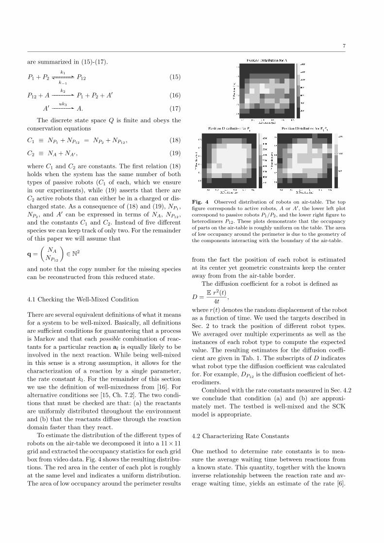
domain faster than they react.To estimate the distribution of the different types of

robots on the air-table we decomposed it into a 11× 11

grid and extracted the occupancy statistics for each grid

box from video data. Fig. 4 shows the resulting distribu-tions. The red area in the center of each plot is roughly

at the same level and indicates a uniform distribution.

The area of low occupancy around the perimeter results

Fig. 4 Observed distribution of robots on air-table. The topfigure corresponds to active robots, A or A′, the lower left plotcorrespond to passive robots P1/P2, and the lower right figure toheterodimers P12. These plots demonstrate that the occupancyof parts on the air-table is roughly uniform on the table. The area

of low occupancy around the perimeter is due to the geometry ofthe components interacting with the boundary of the air-table.

from the fact the position of each robot is estimated

at its center yet geometric constraints keep the center

away from from the air-table border.The diffusion coefficient for a robot is defined as

D =E r2(t)

4t,

where r(t) denotes the random displacement of the robot

as a function of time. We used the targets described in

Sec. 2 to track the position of different robot types.We averaged over multiple experiments as well as the

instances of each robot type to compute the expected

value. The resulting estimates for the diffusion coeffi-

cient are given in Tab. 1. The subscripts of D indicateswhat robot type the diffusion coefficient was calculated

for. For example, DP12is the diffusion coefficient of het-

erodimers.Combined with the rate constants measured in Sec. 4.2

we conclude that condition (a) and (b) are approxi-

mately met. The testbed is well-mixed and the SCKmodel is appropriate.

4.2 Characterizing Rate Constants

One method to determine rate constants is to mea-

sure the average waiting time between reactions froma known state. This quantity, together with the known

inverse relationship between the reaction rate and av-

erage waiting time, yields an estimate of the rate [6].

8

Although useful in simulation, one drawback of this

method is that one needs to repeatedly re-initialize thesystem to gather statistical data, which is tedious and

time consuming. An exception is k3, which was mea-

sured in this way. The reason is that the recharge reac-tion represents a change in internal state, which is easy

to re-initialize.

For the other rate constants we take a different ap-proach. We average multiple longer trajectories all start-

ing from the same initial condition. However, the sys-

tem is allowed to continue evolving for a set amount of

time, possibly undergoing many reactions. This has theadvantage that each re-initialization gives much more

information than a single waiting time. We then fit this

empirical average to solutions of the CME (2).

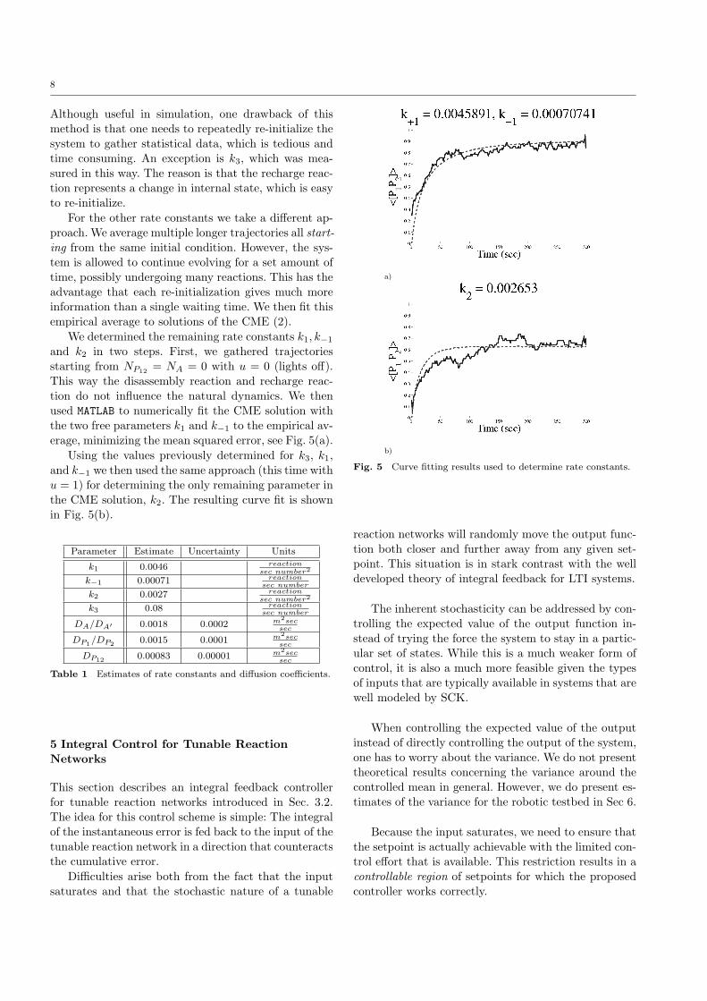
We determined the remaining rate constants k1, k−1

and k2 in two steps. First, we gathered trajectories

starting from NP12= NA = 0 with u = 0 (lights off).

This way the disassembly reaction and recharge reac-

tion do not influence the natural dynamics. We then

used MATLAB to numerically fit the CME solution with

the two free parameters k1 and k−1 to the empirical av-erage, minimizing the mean squared error, see Fig. 5(a).

Using the values previously determined for k3, k1,

and k−1 we then used the same approach (this time withu = 1) for determining the only remaining parameter in

the CME solution, k2. The resulting curve fit is shown

in Fig. 5(b).

Parameter Estimate Uncertainty Units

k1 0.0046 reaction

sec number2

k−1 0.00071 reaction

sec number

k2 0.0027 reaction

sec number2

k3 0.08 reaction

sec number

DA/DA′ 0.0018 0.0002 m2sec

sec

DP1/DP2

0.0015 0.0001 m2sec

sec

DP120.00083 0.00001 m

2sec

sec

Table 1 Estimates of rate constants and diffusion coefficients.

5 Integral Control for Tunable Reaction

Networks

This section describes an integral feedback controllerfor tunable reaction networks introduced in Sec. 3.2.

The idea for this control scheme is simple: The integral

of the instantaneous error is fed back to the input of the

tunable reaction network in a direction that counteractsthe cumulative error.

Difficulties arise both from the fact that the input

saturates and that the stochastic nature of a tunable

a)

b)

Fig. 5 Curve fitting results used to determine rate constants.

reaction networks will randomly move the output func-

tion both closer and further away from any given set-

point. This situation is in stark contrast with the welldeveloped theory of integral feedback for LTI systems.

The inherent stochasticity can be addressed by con-

trolling the expected value of the output function in-

stead of trying the force the system to stay in a partic-ular set of states. While this is a much weaker form of

control, it is also a much more feasible given the types

of inputs that are typically available in systems that arewell modeled by SCK.

When controlling the expected value of the output

instead of directly controlling the output of the system,

one has to worry about the variance. We do not presenttheoretical results concerning the variance around the

controlled mean in general. However, we do present es-

timates of the variance for the robotic testbed in Sec 6.

Because the input saturates, we need to ensure that

the setpoint is actually achievable with the limited con-trol effort that is available. This restriction results in a

controllable region of setpoints for which the proposed

controller works correctly.

9

+

−

1

sSCKy∗ y(q)

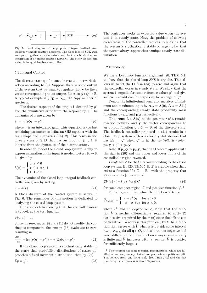
Fig. 6 Block diagram of the proposed integral feedback con-troller for tunable reaction networks. The block labeled SCK withan input, together with the saturation block is a block diagram

description of a tunable reaction network. The other blocks forma simple integral feedback controller.

5.1 Integral Control

The discrete state q of a tunable reaction network de-

velops according to (5). Suppose there is some outputof the system that we want to regulate. Let y be the a

vector corresponding to an output function y : Q→ R.

A typical example is y(q) = NSi, the copy number of

species Si.The desired setpoint of the output is denoted by y∗

and the cumulative error from the setpoint by x. The

dynamics of x are given by

x = γ(y(q) − y∗), (20)

where γ is an integrator gain. This equation is the last

remaining parameter to define an SHS together with the

reset maps and intensities (9)-(12). This constructiongives a class of SHS that has an input u ∈ [0, 1] it

inherits from the dynamics of the discrete states.

In order to model the closed loop system, a way toexpress saturation of the input is needed. Let h : R → R

be given by

h(x) =

0, x ≤ 0

x, 0 < x ≤ 11, 1 < x.

The dynamics of the closed loop integral feedback con-

troller are given by setting

u = h(x). (21)

A block diagram of the control system is shown in

Fig. 6. The remainder of this section is dedicated to

analyzing the closed loop system.Our approach to showing that this controller works

is to look at the test function

ψ(q, x) = x.

Since the reset maps (9) and (11) do not modify the con-tinuous component, the sum in (13) evaluates to zero,

resulting in

dEx

dt= Eγ(y(q) − y∗)) = γ(Ey(q) − y∗). (22)

If the closed loop system is stochastically stable, in

the sense that probability distributions of states ap-

proaches a fixed invariant distribution, then by (22)

Ey = y∗. (23)

The controller works in expected value when the sys-

tem is in steady state. Now, the problem of showingcorrectness of the controller reduces to showing that

the system is stochastically stable or ergodic, i.e. that

the system always approaches a unique steady state dis-tribution.

5.2 Ergodicity

We use a Lyapunov function argument [20, THM 5.1]

to show that the closed loop SHS is ergodic. This al-

lows us to set the LHS in (34) to zero and argue thatthe controller works in steady state. We show that the

system is ergodic for some reference values y∗ and give

sufficient conditions for ergodicity for a range of y∗.Denote the infinitesimal generator matrices of mini-

mum and maximum input by Am = A(0), AM = A(1)

and the corresponding steady state probability mass

functions by pm and pM respectively.Theorem: Let A(u) be the generator of a tunable

reaction network and y the vector corresponding to

an output function y : Q → R of the discrete state.The feedback controller proposed in (21) results in a

closed loop system with a stationary distribution that

has Ey = y∗ when y∗ is in the controllable region,pMy < y∗ < pmy.

Note: If pMy > pmy, then the theorem applies with

the sign in (20) and the upper and lower limits of the

controllable region reversed.Proof: Let Z be the SHS corresponding to the closed

loop system. By [20, THM 5.1], Z is ergodic when there

exists a function V : Z → R+ with the property that

V (z) → ∞ as |z| → ∞ and

LV (z) ≤ −f(z) ∀z /∈ C (24)

for some compact region C and positive function f . 1

For our system, we define the function V to be

V (q, x) =

{x+ c+(q) for x > 0

−x+ c−(q) for x < 0,

where c+ and c− depend on q. Note that the func-

tion V is neither differentiable (required to apply L)nor positive (required by theorem) since the offsets can

be negative. To address this problem, let V be a func-

tion that agrees with V when x is outside some interval[vmin, vmax] for all q ∈ Q, and is both non-negative and

twice differentiable. This function always exists since Q

is finite and V increases with |x| so that V is positivefor sufficiently large |x|.

1 The theorem has some technical preconditions, which are ful-filled in our case, namely that all compact sets are petite see [20].This follows from [21, THM 4.1], [19, THM 27.6] and the factthat every Feller process is also a T-process.

10

+

−

y(q) = NP12Error

Signal

1s

Cum

ulative

Error

Sat

ura

ted

Error

Light

Inte

nsity

y∗

air-table(discrete)

Fig. 7 Block diagram of the proposed control system. Only theair-table state and output signal are discrete, all other signals arecontinuous.

Let the compact region required by the theorem be

C = Q×[min(vmin, 0),max(vmax, 1)]. Since we are onlyinterested in V outside C, we look at the cases when the

feedback input is saturated at either u = 0 or u = 1.

This situation simplifies the analysis, since the tran-sition intensities λ(q, x) are independent of x in the

saturated regions. We now argue that for some range

of setpoints y∗ we can find c+ and c− to make V aLyapunov function in the sense of (24).

Choosing f = ǫ and considering saturation at u = 1first, we rewrite the conditions of (24) in vector from,

y − y∗1 + AMc+ ≤ −ǫ1. (25)

Let ǫ be an arbitrary vector with strictly positive en-

tries, then (25) can be rewritten as

y − y∗1 + AMc+ = −ǫ. (26)

We want to determine when this equation has a solution

for c+. Note that

AMc+ = −ǫ+ y∗1 − y

has a solution only if (−ǫ + y∗1 − y) is in the column

space of AM , which we write (−ǫ+y∗1−y) ∈ ColAM .

Equivalently

(ColAM )⊥ ⊥ (−ǫ+ y∗1 − y) (27)

(NulATM ) ⊥ (−ǫ+ y∗1 − y) (28)

(pM )T ⊥ (−ǫ+ y∗1 − y) (29)

0 = pM (−ǫ+ y∗1 − y) (30)

0 = −pM ǫ+ y∗ − pMy, (31)

where Nul denotes the right null space and a superscript⊥ the orthogonal complement. Because ǫ has arbitrary,

strictly positive entries and entries and pM has non-

negative entries by definition a solution for c+ exists

when

pMy < y∗.

Similarly, for saturation with u = 0 we get

pmy > y∗.

Thus the system is ergodic if

pMy < y∗ < pmy. (32)

NP −1

NA−1

= (NP12−y*)

k2

.x

NP NA

k−1NP

k1NPC12−( )

k3 NAC2−( )h

NP

NA−1

= (NP −y*).x

NP +1

NA−1

= (NP −y*).x

12

12

12

12

12

12

12

12

x( )

NP −1

NA

= (NP12−y*

.x

NP

NA

= (NP −y*).x

NP +1

NA

= (NP −y*).x

12 12

12

12

12

NP −1

NA+1

= (NP12−y*

.x

NP

NA+1

= (NP −y*).x

NP +1

NA+1

= (NP −y*).x

12 12

12

12

12

)

)γ γγ

γ γ

γ γγ

γ

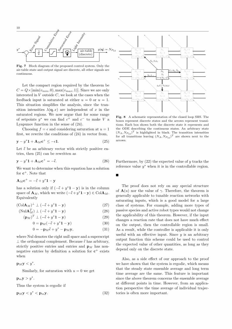
Fig. 8 A schematic representation of the closed loop SHS. Theboxes represent discrete states and the arrows represent transi-

tions. Each box shows both the discrete state it represents andthe ODE describing the continuous states. An arbitrary state(NA, NP12

)T is highlighted in black. The transition intensities

for all transitions leaving (NA, NP12)T are shown next to the

arrows.

Furthermore, by (22) the expected value of y tracks the

reference value y∗ when it is in the controllable region.

The proof does not rely on any special structureof A(u) nor the value of γ. Therefore, the theorem is

generally applicable to tunable reaction networks with

saturating inputs, which is a good model for a largeclass of systems. For example, adding more types of

passive species and active robot types would not change

the applicability of this theorem. However, if the input

changes a reaction rate that does not have much effecton the output, then the controllable region is small.

As a result, while the controller is applicable it is only

useful with an effective input. Since y is an arbitraryoutput function this scheme could be used to control

the expected value of other quantities, as long as they

depend only on the discrete state.

Also, as a side effect of our approach to the proofwe have shown that the system is ergodic, which means

that the steady state ensemble average and long term

time average are the same. This feature is important

since the above theorem concerns the ensemble averageat different points in time. However, from an applica-

tion perspective the time average of individual trajec-

tories is often more important.

11

6 Integral Control Applied to the Robotic

Testbed

This section combines the mathematical model of therobotic testbed developed in Sec. 4 with the results from

the previous section to solve the control problem stated

in Sec. 1.With the mathematical model for the testbedin place we can state the problem more formally. Con-

trol the system such that ENP12= y∗ by adjusting the

intensity of the overhead lamps.

To apply the theorem from from Sec. 5 let the out-

put function y : Q→ R be given by

y(q) = NP12.

The resulting feedback controller is shown in Fig. 7. The

closed loop SHS is characterized by the state transition

diagram shown in Fig. 8 and the extended generator ofthe closed loop SHS

L ψ(NP12, NA, x) (33)

=∂ψ(NP12

, NA, x)

∂xγ(NP12

− y∗)

+ (ψ(NP12+ 1, NA, x) − ψ(NP12

, NA, x))k1(C1 −NP12)2

+ (ψ(NP12− 1, NA, x) − ψ(NP12

, NA, x))k−1NP12

+ (ψ(NP12− 1, NA − 1, x) − ψ(NP12

, NA, x))k2NP12NA

+ (ψ(NP12, NA + 1, x) − ψ(NP12

, NA, x))x(C2 −NA).

As argued in Sec. 5 (22)-(23) setting ψ = x gives

d Ex

dt= E γ(NP12

− y∗), (34)

resulting in correct behavior when the process is er-

godic.

6.1 Experimental Results

We implemented the proposed controller on the robotic

testbed described in Sec. 2. The generator matrix A(u)is defined by (15)-(17) with the parameters found in

Sec. 4. In the following experiments the number of P1

and P2 pairs is C1 = 10 and the number of active robotsis C2 = 4.

To show the controller’s the tracking capability we

tracked two periods of a square wave. The low and highsetpoints were 0.7 and 0.8 (corresponding to 7 and 8

P12). Both of the setpoints are inside the empirically de-

termined controllable region for this system, 0.60-0.86.

To determine the upper and lower limits of the con-

trollable region, the system was operated in open loop

with both u = 0 and u = 1 and allowed to equilibrate.After reaching equilibrium the expected value of the

output function NP12was estimated, which by (32) are

the upper and lower limits of the controllable region.

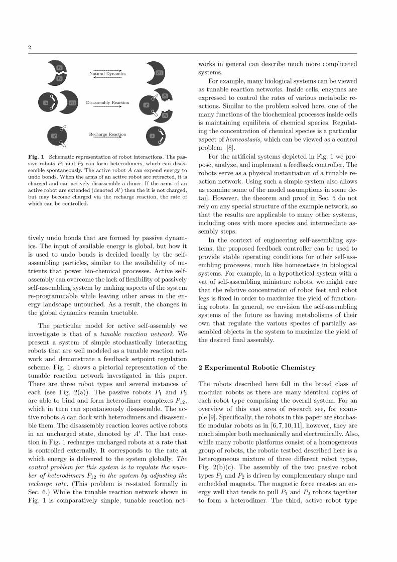
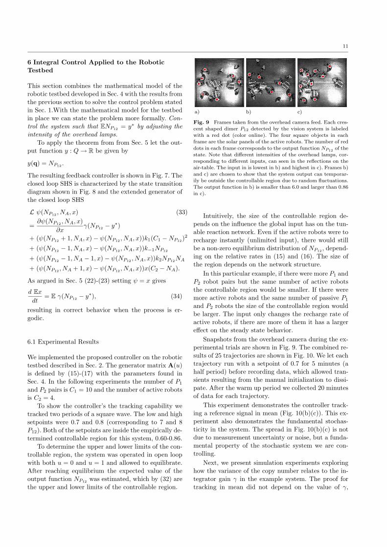
a) b) c)

Fig. 9 Frames taken from the overhead camera feed. Each cres-

cent shaped dimer P12 detected by the vision system is labeledwith a red dot (color online). The four square objects in eachframe are the solar panels of the active robots. The number of reddots in each frame corresponds to the output function NP12

of the

state. Note that different intensities of the overhead lamps, cor-responding to different inputs, can seen in the reflections on theair-table. The input in is lowest in b) and highest in c). Frames b)

and c) are chosen to show that the system output can temporar-ily be outside the controllable region due to random fluctuations.The output function in b) is smaller than 6.0 and larger than 0.86in c).

Intuitively, the size of the controllable region de-

pends on the influence the global input has on the tun-able reaction network. Even if the active robots were to

recharge instantly (unlimited input), there would still

be a non-zero equilibrium distribution of NP12, depend-

ing on the relative rates in (15) and (16). The size of

the region depends on the network structure.

In this particular example, if there were more P1 andP2 robot pairs but the same number of active robots

the controllable region would be smaller. If there were

more active robots and the same number of passive P1

and P2 robots the size of the controllable region wouldbe larger. The input only changes the recharge rate of

active robots, if there are more of them it has a larger

effect on the steady state behavior.

Snapshots from the overhead camera during the ex-

perimental trials are shown in Fig. 9. The combined re-

sults of 25 trajectories are shown in Fig. 10. We let eachtrajectory run with a setpoint of 0.7 for 5 minutes (a

half period) before recording data, which allowed tran-

sients resulting from the manual initialization to dissi-pate. After the warm up period we collected 20 minutes

of data for each trajectory.

This experiment demonstrates the controller track-ing a reference signal in mean (Fig. 10(b)(c)). This ex-

periment also demonstrates the fundamental stochas-

ticity in the system. The spread in Fig. 10(b)(c) is not

due to measurement uncertainty or noise, but a funda-mental property of the stochastic system we are con-

trolling.

Next, we present simulation experiments exploringhow the variance of the copy number relates to the in-

tegrator gain γ in the example system. The proof for

tracking in mean did not depend on the value of γ,

12

b) c)

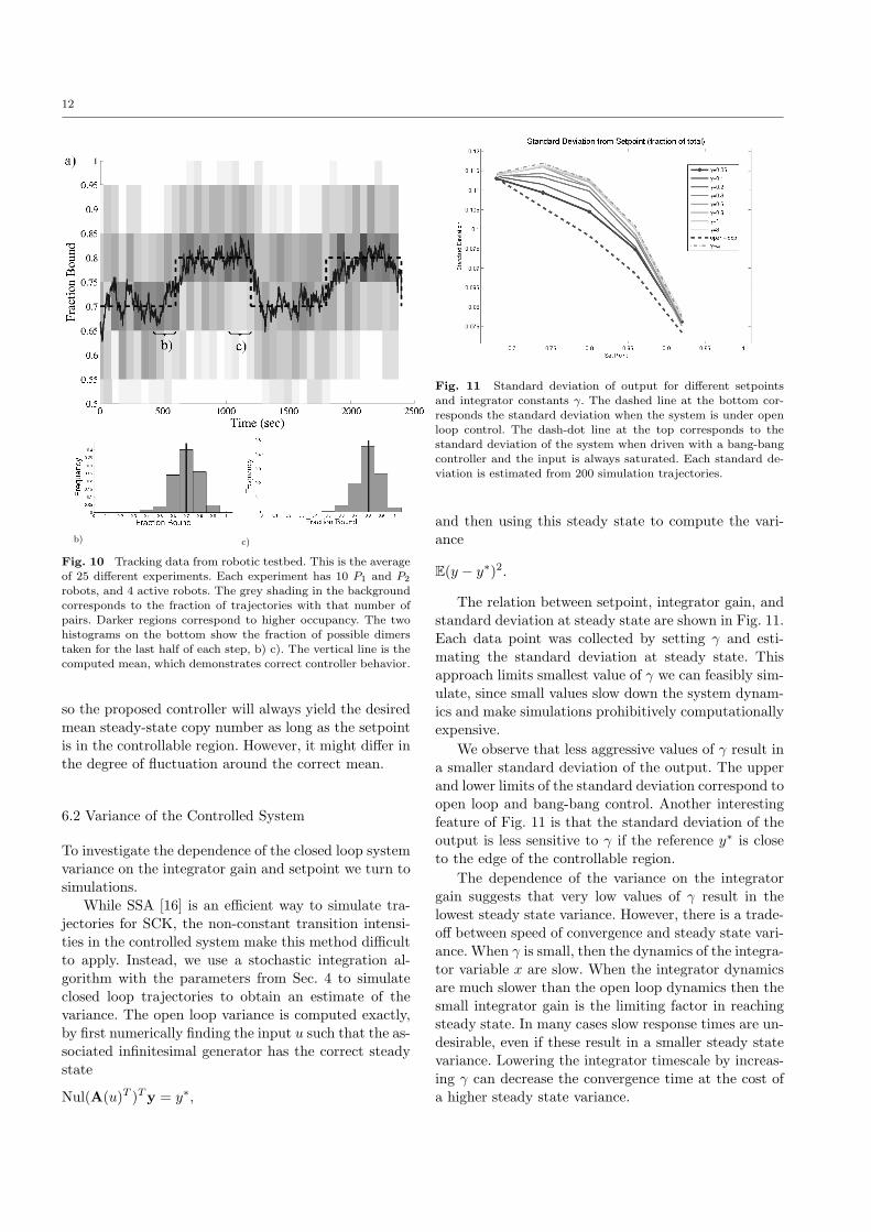
Fig. 10 Tracking data from robotic testbed. This is the average

of 25 different experiments. Each experiment has 10 P1 and P2

robots, and 4 active robots. The grey shading in the backgroundcorresponds to the fraction of trajectories with that number ofpairs. Darker regions correspond to higher occupancy. The two

histograms on the bottom show the fraction of possible dimerstaken for the last half of each step, b) c). The vertical line is thecomputed mean, which demonstrates correct controller behavior.

so the proposed controller will always yield the desiredmean steady-state copy number as long as the setpoint

is in the controllable region. However, it might differ in

the degree of fluctuation around the correct mean.

6.2 Variance of the Controlled System

To investigate the dependence of the closed loop system

variance on the integrator gain and setpoint we turn tosimulations.

While SSA [16] is an efficient way to simulate tra-jectories for SCK, the non-constant transition intensi-

ties in the controlled system make this method difficult

to apply. Instead, we use a stochastic integration al-gorithm with the parameters from Sec. 4 to simulate

closed loop trajectories to obtain an estimate of the

variance. The open loop variance is computed exactly,by first numerically finding the input u such that the as-

sociated infinitesimal generator has the correct steady

state

Nul(A(u)T )T y = y∗,

Fig. 11 Standard deviation of output for different setpointsand integrator constants γ. The dashed line at the bottom cor-

responds the standard deviation when the system is under openloop control. The dash-dot line at the top corresponds to thestandard deviation of the system when driven with a bang-bangcontroller and the input is always saturated. Each standard de-

viation is estimated from 200 simulation trajectories.

and then using this steady state to compute the vari-

ance

E(y − y∗)2.

The relation between setpoint, integrator gain, andstandard deviation at steady state are shown in Fig. 11.

Each data point was collected by setting γ and esti-

mating the standard deviation at steady state. This

approach limits smallest value of γ we can feasibly sim-ulate, since small values slow down the system dynam-

ics and make simulations prohibitively computationally

expensive.

We observe that less aggressive values of γ result in

a smaller standard deviation of the output. The upper

and lower limits of the standard deviation correspond toopen loop and bang-bang control. Another interesting

feature of Fig. 11 is that the standard deviation of the

output is less sensitive to γ if the reference y∗ is close

to the edge of the controllable region.

The dependence of the variance on the integrator

gain suggests that very low values of γ result in the

lowest steady state variance. However, there is a trade-off between speed of convergence and steady state vari-

ance. When γ is small, then the dynamics of the integra-

tor variable x are slow. When the integrator dynamicsare much slower than the open loop dynamics then the

small integrator gain is the limiting factor in reaching

steady state. In many cases slow response times are un-

desirable, even if these result in a smaller steady statevariance. Lowering the integrator timescale by increas-

ing γ can decrease the convergence time at the cost of

a higher steady state variance.

13

Note, that the controllable region in the simulated

system is shifted up from the physical system. This islikely due to the charging behavior of the active robots,

which is modeled as exponential in the simulation, but

actually has a different distribution. Each disassemblytakes roughly the same amount of energy. However, re-

gardless of the exact location of the controllable region,

we expect the qualitative behavior of the variance tobe similar, especially since the network structure is the

same. What is important about the controllable region

is that setpoints inside it can be reached.

7 Conclusions and Future Work

We proposed an integral feedback controller for control-ling the average copy number of an arbitrary species in

a system modeled as a tunable reaction network. We

prove that the controller tracks a reference in mean anddemonstrate the approach on an robotic experimental

platform. We also present some preliminary simulation

results regarding the variance of the copy number as

a function of the integrator gain and setpoint. We arecurrently working on analytical results describing the

steady state variance of the control scheme.

Finally, we would like to emphasize the generality of

our approach. This control scheme works for any tun-able reaction network and requires no tweaking of the

integrator gain γ as long as the reference is in the con-

trollable region, which is easy to measure experimen-

tally. Also, the tunable reaction network model is quitegeneral since the variable rate input can model a wide

variety of physical mechanisms. While we presented an

example system with relatively large components, webelieve that the presented or similar approaches will

be especially useful in the context of many microscopic

components.

In the future we would like to find ways to decentral-ize the controller by using local estimates of the global

output. In particular, we want to implement this con-

trol scheme with other chemical reactions. For example,

the continuous state could correspond to a high copynumber species where the mass action kinetics approxi-

mation works well. Such an implementation would open

the door to using the proposed control scheme in manyother settings, such as biological systems.

Acknowledgements

We would like to thank Sheldon Rucker, Michael Mc-

Court, and Yi-Wei Li for their dedication and hard work

in designing and building the robots. We would also like

to thank Alexandre Mesquita and Joao Hespanha for

their helpful discussions about proving ergodicity.

References

1. E. Saeedi, S. Kim, H. Ho, and B. A. Parviz, “Self-assembledsingle-digit micro-display on plastic,” in MEMS/MOEMSComponents and Their Applications V. Special Focus Top-ics: Transducers at the Micro-Nano Interface, vol. 6885,

pp. 688509–1 – 688509–12, SPIE, 2008.

2. P. W. K. Rothemund, “Folding dna to create nanoscaleshapes and patterns,” Nature, vol. 440, pp. 297–302, Mar.

2006.

3. M. Boncheva, D. A. Bruzewicz, and G. M. Whitesides,

“Millimeter-scale self-assembly and its applications,” PureAppl. Chem, vol. 75, pp. 621–630, 2003.

4. H. Onoe, K. Matsumoto, and I. Shimoyama, “Three-

dimensional micro-self-assembly using hydrophobic interac-tion controlled by self-assembled monolayers,” Microelec-tromechanical Systems, Journal of, vol. 13, pp. 603–611,

Aug. 2004.

5. Massimo, Mastrangeli, S. Abbasi, agdas Varel, C. van Hoof,C. Celis, and K. F. Bhringer, “Self-assembly from milli tonanoscales: Methods and applications,” IOP Journal of Mi-cromechanics and Microengineering, vol. 19, no. 8, p. 37pp,2009.

6. S. Burden, N. Napp, and E. Klavins, “The statistical dy-namics of programmed robotic self-assembly,” in ConferenceProceedings ICRA 06, pp. 1469–76, 2006.

7. P. J. White, K. Kopanski, and H. Lipson, “Stochastic self-reconfigurable cellular robotics,” IEEE International Con-ference on Robotics and Automation (ICRA04), pp. 2888–

2893, 2004.

8. H. El-Samad, J. P. Goff, and M. Khammash, “Calciumhomeostasis and parturient hypocalcemia: An integral feed-

back perspective,” Journal of Theoretical Biology, vol. 214,pp. 17–29, Jan. 2002.

9. M. Yim, W. Shen, B. Salemi, D. Rus, M. Moll, H. Lipson,

E. Klavins, and G. Chirikjian, “Modular self-reconfigurablerobot systems,” IEEE Robotics Automation Magazine,vol. 14, pp. 43 –52, march 2007.

10. P. White, V. Zykov, J. Bongard, and H. Lipson, “Three di-mensional stochastic reconfiguration of modular robots,” inProceedings of Robotics Science and Systems, (Cambridge

MA), June 2005.

11. N. Ayanian, P. White, A. Halasz, M. Yim, and V. Kumar,“Stochastic control for self-assembly of XBots,” in ASME

Mechanisms and Robotics Conference, (New York), August2008.

12. B. Donald, C. Levey, I. Paprotny, and D. Rus, “Simultane-ous control of multiple mems microrobots,” in The EighthInternational Workshop on the Algorithmic Foundations ofRobotics (WAFR), December 2008.

13. D. A. McQuarrie, “Stochastic approach to chemical kinet-ics,” Journal of Applied Probability, vol. 4, pp. 413–478, Dec1967.

14. K. Hosokawa, I. Shimoyama, and H. Miura., “Dynamics ofself assembling systems: Analogy with chemical kinetics,” Ar-

tificial Life, vol. 1, no. 4, pp. 413–427, 1994.

15. N. V. Kampen, Stochastic Processes in Physics and Chem-istry. Elsevier, 3rd ed., 2007.

16. D. T. Gillespie, “Exact stochastic simulation of coupledchemical reactions,” Journal of Physical Chemistry, vol. 81,no. 25, pp. 2340–2361, 1977.

14

17. J. P. Hespanha, “Modeling and analysis of stochastic hybridsystems,” IEE Proc — Control Theory & Applications, Spe-cial Issue on Hybrid Systems, vol. 153, no. 5, pp. 520–535,

2007.18. J. P. Hespanha and J. Abhyudai, “Stochastic models for

chemically reacting systems using polynomial hybrid sys-

tems,” International Journal of Robust and Nonlinar Con-trol, vol. 15, no. 15, pp. 669 – 689, 2005.

19. M. Davis, Markov Processes and Optimization. Chapman &Hall, 1993.

20. S. P. Meyn and R. L. Tweedie, “Stability of Markovianprocesses III: Foster-lyapunov criteria for continuous-timeprocesses,” Advances in Applied Probability, vol. 25, no. 3,pp. 518–548, 1993.

21. S. P. Meyn and R. L. Tweedie, “Stability of Markovian pro-cesses II: Continuous-time processes and sampled chains,”Advances in Applied Probability, vol. 25, no. 3, pp. 487–517,

1993.