PHYSICAL REVIEW E 94, 052218 (2016)

Statistics of the stochastically forced Lorenz attractor by the Fokker-Planckequation and cumulant expansions

Altan Allawala* and J. B. Marston†

Department of Physics, Box 1843, Brown University, Providence, Rhode Island 02912-1893, USA(Received 7 April 2016; revised manuscript received 18 October 2016; published 23 November 2016)

We investigate the Fokker-Planck description of the equal-time statistics of the three-dimensional Lorenzattractor with additive white noise. The invariant measure is found by computing the zero (or null) mode ofthe linear Fokker-Planck operator as a problem of sparse linear algebra. Two variants are studied: a self-adjointconstruction of the linear operator and the replacement of diffusion with hyperdiffusion. We also access thelow-order statistics of the system by a perturbative expansion in equal-time cumulants. A comparison is madeto statistics obtained by the standard approach of accumulation via direct numerical simulation. Theoretical andcomputational aspects of the Fokker-Planck and cumulant expansion methods are discussed.

DOI: 10.1103/PhysRevE.94.052218

I. INTRODUCTION

Chaotic dynamical systems often have a well-definedstatistical steady state. Traditionally statistics are estimated bytheir accumulation through direct numerical simulation (DNS)starting from an ensemble of initial conditions. If the basinof attraction is ergodic, ensemble averaging can be replacedby time averaging over a single long trajectory. Rare butlarge deviations may occur, however, necessitating extremelylong integration times. An alternative and more efficientapproach solves for the statistics directly. Depending on thequestion to be answered, such direct statistical simulation(DSS) can focus on various statistical quantities such as theprobability distribution function (PDF) or invariant measure,the low-order equal-time moments, autocorrelations in time,or large deviations.

This paper presents two different types of DSS. The first,the Fokker-Planck equation (FPE), describes the flow ofprobability density in phase space, respecting the conservationof total probability. Consider a trajectory governed by thedifferential equation

d �xdt

= �V (�x) + �η(t), (1)

where �η(t) is additive stochastic forcing. The FPE for thissystem is

∂P (�x,t)

∂t= −LFPEP (�x,t), (2)

where we will call LFPE the (linear) FPE operator. Theplacement of the negative sign in front of the operatorLFPE in Eq. (2) is for convenience: The operator LFPE isthen semipositive definite and the steady-state statistics aredetermined by the ground state. In the special case where �η isGaussian additive white noise with no mean and covariancegiven by

〈ηi(t)ηj (t ′)〉 = 2�ij δ(t − t ′), (3)

*allawala@brown.edu†marston@brown.edu

with angular brackets indicating a short time average, only afinite number of terms appear in the FPE operator [1]:

LFPEP = �∇ · ( �V P ) − �∇2P. (4)

Additive stochastic forcing smears out the PDF P throughdiffusion in phase space. A canonical example is the one-dimensional Ornstein-Uhlenbeck process with trajectoriesgoverned by

x = −ax + η(t). (5)

The corresponding FPE is

∂P (x,t)

∂t= ∂

∂x[axP (x,t)] + �

∂2P (x,t)

∂x2, (6)

which has a steady-state solution that is readily found to beGaussian:

P (x) =√

a

2π�e−ax2/2�. (7)

As we will see, stochastic forcing also needs to be introducedto regulate strange attractors at small scales. As the fractalstructure of a strange attractor cannot be resolved on a lattice,it is necessary to smooth the structure at the lattice length scale.We use additive stochastic forcing for this purpose.

Direct solution of the FPE is most commonly carried out forone-dimensional systems. Extension to higher dimensions isconceptually straightforward, but numerically challenging [2].The objective of the present paper is to apply the FPE to a three-dimensional chaotic system. Numerical solutions have beendeveloped based on finite elements [3,4], finite differences [5],and path integrals [6]. Here we depart from these traditionalmethods by instead directly solving for the zero or null modeof a finite-difference discretized FPE operator, thus obviatingthe time-consuming and costly steps of computing the transientprobability distributions. We illustrate this method by applyingit to the Lorenz system [7] with additive stochastic forcing.Although a phenomenological FPE has been applied for aquantum system without the addition of stochastic forcing [8],we follow previous work [9–13] and add small additive whitenoise to wash out fractal structure below the lattice scale.

Since numerical solution of the FPE in larger numbers ofdimensions is stymied by the “curse of dimensionality,” it is

2470-0045/2016/94(5)/052218(9) 052218-1 ©2016 American Physical Society

ALTAN ALLAWALA AND J. B. MARSTON PHYSICAL REVIEW E 94, 052218 (2016)

important to develop alternative forms of DSS. Accordingly,we also explore a second type of DSS, an expansion inequal-time cumulants that can be applied to high-dimensionaldynamical systems. A cumulant expansion was employed forthe Orszag-McLaughlin attractor in Ref. [14]. For the Lorenzattractor we show that low-order statistics are well reproducedat third-order truncation.

The paper is organized as follows. Section II briefly de-scribes the Lorenz system with additive stochastic forcing andits numerical integration. Two different sets of parameters areconsidered, both of which yield chaotic behavior. Section IIIdescribes the FPE and the numerical method that we use tofind the invariant measure. Equal-time statistics so obtainedare compared to those found through accumulation by DNS.We study the scaling of the spectral gap of the linear FPEoperator as the stochastic forcing is varied. Two extensionsto the method are also considered: a self-adjoint constructionof the linear operator and the replacement of diffusion withhyperdiffusion. Section IV presents the cumulant expansiontechnique and its evaluation by comparison to DNS. Asummary is presented in Sec. V.

II. LORENZ ATTRACTOR WITH ADDITIVESTOCHASTIC FORCING

The Lorenz attractor is a three-dimensional chaotic systemthat was originally derived by applying a severe Galerkin ap-proximation to the equations of motion (EOMs) for Rayleigh-Benard convection with stress-free boundary conditions [7].We study an extension with additive stochastic forcing [9–13]that obeys Eq. (3). Such additive white noise can model fast orunresolved physical processes that are not explicitly described,

x = σ (y − x) + η1(t),

y = x(ρ − z) − y + η2(t),

z = xy − βz + η3(t). (8)

In this context x is proportional to convective intensity,y to the difference in temperature between ascending anddescending currents, and z to the vertical temperature profile’sdeviation from linearity. The parameters β, ρ, and σ area geometric factor, the Rayleigh number, and the Prandtlnumber, respectively. We also choose the covariance of theGaussian white noise to be diagonal and isotropic: �ij = �δij .

We study the strange attractor at two different sets ofparameters. The conventional (classic) parameters are β =1.0, ρ = 26.5, and σ = 3.0. We also examine the case withthe geometric factor changed to β = 0.16. This modificationenhances layering in the PDF. Since the geometric factor isrelated to the size of the attractor, a reduction in β shrinks theattractor, which in turn allows for a reduction in the stochasticforcing while keeping the structure sufficiently smooth atthe lattice length scale. The attractors have two prominentwings (see Fig. 1). Transitions between the two wings arecharacterized by a long time scale, whereas orbits within eachwing occur on a fast time scale of order τ ≈ 1.

Direct numerical simulation

The EOMs (8) are integrated forward in time with thefourth-order accurate Runge-Kutta algorithm with fixed time

step δt = 0.01. Stochastic forcing, drawn from a normal dis-tribution, is updated at intervals of �t = 0.1 and interpolatedat intermediate times δt . Note that there is a good separationof time scales with τ � �t � δt following the reasoning ofRef. [15].

Statistics are accumulated up to a final time T = 2 × 107.The PDF is estimated from the histogram that results frombinning the trajectory into cubic boxes. The PDF is projectedonto a plane by integrating over the direction perpendicular tothe plane, for instance,

P (x,y) =∫ ∞

−∞P (x,y,z)dz. (9)

Figures 1, 3, and 5 show that even small stochastic forcingsmoothes out the fine structure of the strange attractor [16]; inparticular, the ringlike steps in the PDF disappear.

III. FOKKER-PLANCK EQUATION

The FPE is an attractive alternative to the accumulationof statistics by DNS. The linear FPE operator for the Lorenzsystem

LFPEP = �∇ · {[σ (y − x),x(ρ − z)

− y,xy − βz]P ]} − �∇2P (10)

is positive-definite in the sense that the real part of theeigenvalues are non-negative [if that were not the case, Eq. (2)would diverge]. The equal-time PDF of the FPE is the zero ornull mode of LFPE. By discretizing the operator on a lattice,the problem of finding the zero mode is converted to a problemof sparse linear algebra.

A. Numerical solution

A standard center-difference scheme is used to discretizethe derivatives that appear in Eq. (10):

f ′i ≈ fi+1 − fi−1

2�x,

f ′′i ≈ fi+1 − 2fi + fi−1

�x2. (11)

The PDF of the unforced Lorenz attractor has compactsupport, but once stochastic forcing is included the PDF isnonzero but exponentially small throughout phase space. Inthe numerical calculation, the probability density P is takento vanish outside of the domain. The zero mode of LFPE isfound with the use of a preconditioned Jacobi-Davidson QR(JDQR) algorithm [17,18] that computes the partial Schurdecomposition of a matrix with error tolerance set to 10−5.We have checked that our results do not change appreciablyfor tighter tolerances. Although the JDQR algorithm is wellsuited for sparse matrices, requiring only the action of amatrix multiplying a vector, we were unable to find a suitablesparse preconditioner. A sparse preconditioner would enablea substantial increase in resolution. The Jacobi correctionequation is preconditioned following Sec. 3.2 of Ref. [18]and solved using the generalized minimal residual methodusing MATLAB. The highest resolution we have been able toreach is 1603 with 500 GB of memory. This large number ofgrid points for which the Fokker-Planck equation has been

052218-2

STATISTICS OF THE STOCHASTICALLY FORCED . . . PHYSICAL REVIEW E 94, 052218 (2016)

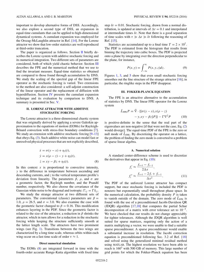
FIG. 1. (a) PDF of the unforced Lorenz system (binned on a 6373 grid) accumulated by DNS. Classic Lorenz parameters are used (seeSec. II). (b) Same as (a), but with added stochastic forcing (� = 0.2) (4783 grid). Note that the fine rings visible in the unforced system arewashed out by the noise. (c) PDF of the stochastically forced attractor (� = 0.2) as obtained from the zero mode of LFPE on a 1603 grid andfor x ∈ [−12.5,12.5], y ∈ [−24,24], and z ∈ [1,45]. The JDQR algorithm is employed. Rows (1), (2), and (3) correspond to the x-y, x-z, andy-z projections of the PDF, respectively. Good agreement between (b) DNS and (c) FPE is evident. Red lines correspond to the cross sectionsshown in Fig. 2.

(a) (b)

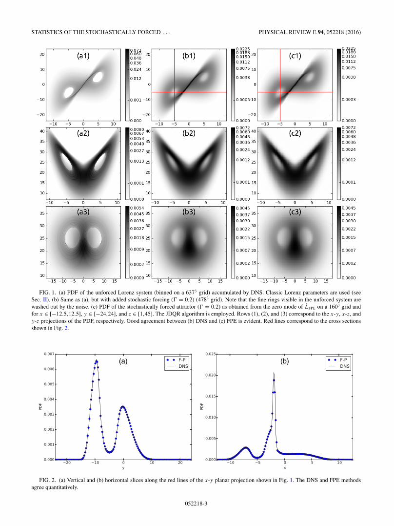
FIG. 2. (a) Vertical and (b) horizontal slices along the red lines of the x-y planar projection shown in Fig. 1. The DNS and FPE methodsagree quantitatively.

052218-3

ALTAN ALLAWALA AND J. B. MARSTON PHYSICAL REVIEW E 94, 052218 (2016)

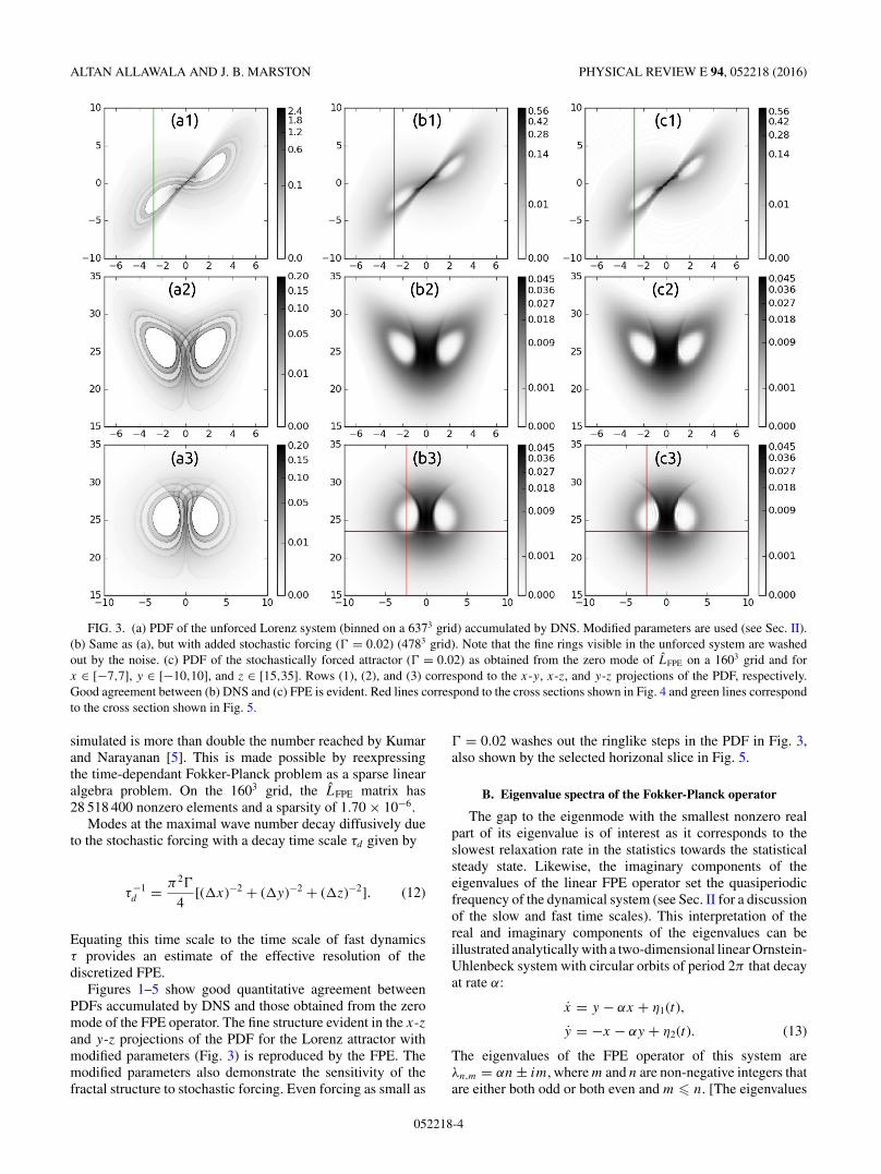
FIG. 3. (a) PDF of the unforced Lorenz system (binned on a 6373 grid) accumulated by DNS. Modified parameters are used (see Sec. II).(b) Same as (a), but with added stochastic forcing (� = 0.02) (4783 grid). Note that the fine rings visible in the unforced system are washedout by the noise. (c) PDF of the stochastically forced attractor (� = 0.02) as obtained from the zero mode of LFPE on a 1603 grid and forx ∈ [−7,7], y ∈ [−10,10], and z ∈ [15,35]. Rows (1), (2), and (3) correspond to the x-y, x-z, and y-z projections of the PDF, respectively.Good agreement between (b) DNS and (c) FPE is evident. Red lines correspond to the cross sections shown in Fig. 4 and green lines correspondto the cross section shown in Fig. 5.

simulated is more than double the number reached by Kumarand Narayanan [5]. This is made possible by reexpressingthe time-dependant Fokker-Planck problem as a sparse linearalgebra problem. On the 1603 grid, the LFPE matrix has28 518 400 nonzero elements and a sparsity of 1.70 × 10−6.

Modes at the maximal wave number decay diffusively dueto the stochastic forcing with a decay time scale τd given by

τ−1d = π2�

4[(�x)−2 + (�y)−2 + (�z)−2]. (12)

Equating this time scale to the time scale of fast dynamicsτ provides an estimate of the effective resolution of thediscretized FPE.

Figures 1–5 show good quantitative agreement betweenPDFs accumulated by DNS and those obtained from the zeromode of the FPE operator. The fine structure evident in the x-zand y-z projections of the PDF for the Lorenz attractor withmodified parameters (Fig. 3) is reproduced by the FPE. Themodified parameters also demonstrate the sensitivity of thefractal structure to stochastic forcing. Even forcing as small as

� = 0.02 washes out the ringlike steps in the PDF in Fig. 3,also shown by the selected horizonal slice in Fig. 5.

B. Eigenvalue spectra of the Fokker-Planck operator

The gap to the eigenmode with the smallest nonzero realpart of its eigenvalue is of interest as it corresponds to theslowest relaxation rate in the statistics towards the statisticalsteady state. Likewise, the imaginary components of theeigenvalues of the linear FPE operator set the quasiperiodicfrequency of the dynamical system (see Sec. II for a discussionof the slow and fast time scales). This interpretation of thereal and imaginary components of the eigenvalues can beillustrated analytically with a two-dimensional linear Ornstein-Uhlenbeck system with circular orbits of period 2π that decayat rate α:

x = y − αx + η1(t),

y = −x − αy + η2(t). (13)

The eigenvalues of the FPE operator of this system areλn,m = αn ± im, where m and n are non-negative integers thatare either both odd or both even and m � n. [The eigenvalues

052218-4

STATISTICS OF THE STOCHASTICALLY FORCED . . . PHYSICAL REVIEW E 94, 052218 (2016)

(a) (b)

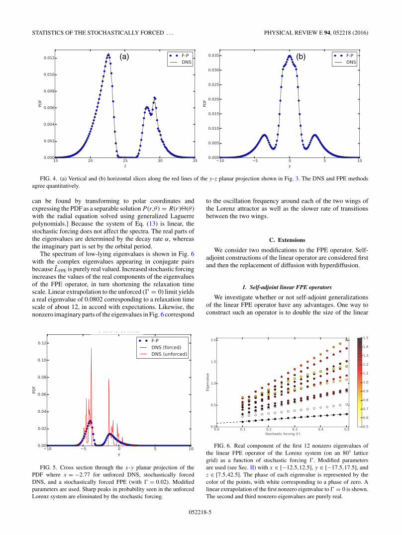
FIG. 4. (a) Vertical and (b) horizontal slices along the red lines of the y-z planar projection shown in Fig. 3. The DNS and FPE methodsagree quantitatively.

can be found by transforming to polar coordinates andexpressing the PDF as a separable solution P (r,θ ) = R(r)�(θ )with the radial equation solved using generalized Laguerrepolynomials.] Because the system of Eq. (13) is linear, thestochastic forcing does not affect the spectra. The real parts ofthe eigenvalues are determined by the decay rate α, whereasthe imaginary part is set by the orbital period.

The spectrum of low-lying eigenvalues is shown in Fig. 6with the complex eigenvalues appearing in conjugate pairsbecause LFPE is purely real valued. Increased stochastic forcingincreases the values of the real components of the eigenvaluesof the FPE operator, in turn shortening the relaxation timescale. Linear extrapolation to the unforced (� = 0) limit yieldsa real eigenvalue of 0.0802 corresponding to a relaxation timescale of about 12, in accord with expectations. Likewise, thenonzero imaginary parts of the eigenvalues in Fig. 6 correspond

FIG. 5. Cross section through the x-y planar projection of thePDF where x = −2.77 for unforced DNS, stochastically forcedDNS, and a stochastically forced FPE (with � = 0.02). Modifiedparameters are used. Sharp peaks in probability seen in the unforcedLorenz system are eliminated by the stochastic forcing.

to the oscillation frequency around each of the two wings ofthe Lorenz attractor as well as the slower rate of transitionsbetween the two wings.

C. Extensions

We consider two modifications to the FPE operator. Self-adjoint constructions of the linear operator are considered firstand then the replacement of diffusion with hyperdiffusion.

1. Self-adjoint linear FPE operators

We investigate whether or not self-adjoint generalizationsof the linear FPE operator have any advantages. One way toconstruct such an operator is to double the size of the linear

FIG. 6. Real component of the first 12 nonzero eigenvalues ofthe linear FPE operator of the Lorenz system (on an 803 latticegrid) as a function of stochastic forcing �. Modified parametersare used (see Sec. II) with x ∈ [−12.5,12.5], y ∈ [−17.5,17.5], andz ∈ [7.5,42.5]. The phase of each eigenvalue is represented by thecolor of the points, with white corresponding to a phase of zero. Alinear extrapolation of the first nonzero eigenvalue to � = 0 is shown.The second and third nonzero eigenvalues are purely real.

052218-5

ALTAN ALLAWALA AND J. B. MARSTON PHYSICAL REVIEW E 94, 052218 (2016)

space by introducing the operator

H2 =(

0 LFPE

L†FPE 0

)(14)

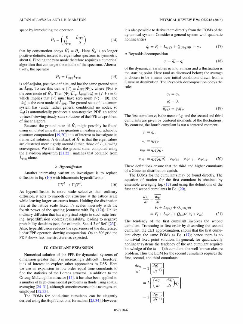
that by construction obeys H†2 = H2. Here H2 is no longer

positive-definite; instead its eigenvalue spectrum is symmetricabout 0. Finding the zero mode therefore requires a numericalalgorithm that can target the middle of the spectrum. Alterna-tively, the operator

H1 ≡ L†FPELFPE (15)

is self-adjoint, positive-definite, and has the same ground stateas LFPE. To see this define |V 〉 ≡ LFPE|�0〉, where |�0〉 isthe zero mode of H1. Then 〈�0|L†

FPELFPE|�0〉 = 〈V |V 〉 = 0,which implies that |V 〉 must have zero norm |V 〉 = |0〉, and|�0〉 is the zero mode of LFPE. The ground state of a quantumsystem has (under rather general conditions) no nodes, so�0(�x) automatically produces a non-negative PDF, an addedvirtue of viewing steady-state solutions of the FPE as a problemof linear algebra.

Because the ground state of H1 might possibly be foundusing simulated annealing or quantum annealing and adiabaticquantum computation [19,20], it is of interest to investigate itsnumerical solution. A drawback of H1 is that the eigenvaluesare clustered more tightly around 0 than those of L, slowingconvergence. We find that the ground state, computed usingthe Davidson algorithm [21,22], matches that obtained fromLFPE alone.

2. Hyperdiffusion

Another interesting variant to investigate is to replacediffusion in Eq. (10) with biharmonic hyperdiffusion:

−�∇2 → �2∇4. (16)

As hyperdiffusion is more scale selective than ordinarydiffusion, it acts to smooth out structure at the lattice scalewhile leaving larger structures intact. Holding the dissipationrate at the lattice scale fixed, �2 scales inversely with thefourth power of the spacing [contrast with Eq. (12)]. Unlikeordinary diffusion that has a physical origin in stochastic forc-ing, hyperdiffusion violates realizability, leading to negativeprobability densities (see, for example, Sec. 4.3 of Ref. [23]).Also, hyperdiffusion reduces the sparseness of the discretizedlinear FPE operator, slowing computation. On an 803 grid thePDF shows less fine structure, as expected.

IV. CUMULANT EXPANSION

Numerical solution of the FPE for dynamical systems ofdimension greater than 3 is increasingly difficult. Therefore,it is of interest to explore other approaches to DSS. Herewe use an expansion in low-order equal-time cumulants tofind the statistics of the Lorenz attractor. In addition to theOrszag-McLaughlin attractor [14], it has also been applied toa number of high-dimensional problems in fluids using spatialaveraging [24–31], although sometimes ensemble averages areemployed [32,33].

The EOMs for equal-time cumulants can be elegantlyderived using the Hopf functional formalism [25,34]. However,

it is also possible to derive them directly from the EOMs of thedynamical system. Consider a general system with quadraticnonlinearities

qi = Fi + Lijqj + Qijkqjqk + ηi. (17)

A Reynolds decomposition

qi = qi + q ′i (18)

of the dynamical variables qi into a mean and a fluctuation isthe starting point. Here (and as discussed below) the averageis chosen to be a mean over initial conditions drawn from aGaussian distribution. The Reynolds decomposition obeys therules

qi = qi,

q ′i = 0,

qiqj = qiqj . (19)

The first cumulant ci is the mean of qi and the second and thirdcumulants are given by centered moments of the fluctuations.By contrast, the fourth cumulant is not a centered moment:

ci ≡ qi,

cij ≡ q ′iq

′j ,

cijk ≡ q ′iq

′j q

′k,

cijk� ≡ q ′iq

′j q

′kq

′� − cij ck� − cikcj� − ci�cjk. (20)

These definitions ensure that the third and higher cumulantsof a Gaussian distribution vanish.

The EOMs for the cumulants may be found directly. Theequation of motion for the first cumulant is obtained byensemble averaging Eq. (17) and using the definitions of thefirst and second cumulants in Eq. (20),

dci

dt= dqi

dt

= Fi + Lijqj + Qijkqjqk

= Fi + Lij cj + Qijk(cj ck + cjk). (21)

The tendency of the first cumulant involves the secondcumulant. Truncating at first order by discarding the secondcumulant, the CE1 approximation, shows that the first cumu-lant obeys the same EOMs as Eq. (17); hence there is nonontrivial fixed point solution. In general, for quadraticallynonlinear systems the tendency of the nth cumulant requiresknowledge of the (n + 1)th cumulant, the well-known closureproblem. Thus the EOM for the second cumulants requires thefirst, second, and third cumulants:

dcij

dt= 2

{dq ′

i

dtq ′

j

}

= 2

{(dqi

dt− dqi

dt

)q ′

j

}

= 2

{dqi

dtq ′

j

}

052218-6

STATISTICS OF THE STOCHASTICALLY FORCED . . . PHYSICAL REVIEW E 94, 052218 (2016)

= 2{Likqkq′j + Qik�qkq�q

′j } + 2�ij

= {2Likckj + Qik�(4ckc�j + 2ck�j )} + 2�ij . (22)

The covariance matrix �ij of the stochastic forcing appearsin the last two lines as (implicitly) a short-time averaginghas been carried out in addition to ensemble averaging. Thesymmetrization operation {· · · } over all permutations of thefree indices has been introduced for conciseness. In the case ofa two-index variable such as the second cumulant it is definedas {cij } = 1

2 (cij + cji) and similarly for higher cumulants.Because each higher cumulant carries an additional di-

mension with it, closure should be performed as soon aspossible. Closing the EOMs at second order by discardingthe contribution of the third cumulant cijk (CE2) is sometimespossible [24] and yields a realizable approximation (becausethe PDF is Gaussian that is non-negative everywhere). TheCE2 EOMs can then be integrated forward in time byspecifying as an initial condition nonzero first and secondcumulants, corresponding to a normally distributed initialensemble. However, the Lorenz attractor is so nonlinear thatthe CE2 EOMs, integrated forward in time, do not reach afixed point that would characterize a statistical steady state.Therefore, we proceed to next order, CE3, by setting thefourth cumulant to zero, cijkl = 0. The fourth centered momentmay then be expressed in terms of the second and thirdcumulants

q ′mq ′

nq′j q

′k = cmncjk + cmj cnk + cmkcjn + cmnjk

cmncjk + cmj cnk + cmkcjn (CE3) (23)

and the EOM for the third cumulant now closes:

dcijk

dt= 3

{dq ′

i

dtq ′

j q′k

}

= 3

{(dqi

dt− dqi

dt

)q ′

j q′k

}

= 3

{dqi

dtq ′

j q′k − dci

dtq ′

j q′k

}

= 3{Limcmjk + Qimn(2cmcnjk − cmncjk + q ′mq ′

nq′j q

′k)}

= {3Limcmjk + 6Qimn(cmcnjk + cmj cnk)} − cijk

τd

.

(24)

In the final line of Eq. (24) a phenomenological eddy dampingtime scale τd has been introduced to model the neglect ofthe fourth cumulant [30,35]. CE2 is recovered in the limitτd → 0 as the third cumulant is suppressed in this limit.As τd is increased, contributions from the interactions oftwo fluctuations that produce another fluctuation begin to befelt. These nonlinear fluctuation + fluctuation → fluctuationinteractions are dropped at order CE2, which retains only thefluctuation + fluctuation → mean and fluctuation + mean →fluctuation interactions [30]. This can be seen by examiningEqs. (21) and (22) and observing that the second cumulantonly interacts through Qijk with the first cumulant, andnot with itself. Upon increasing τd further, eventually re-alizability is lost as the second cumulant develops negative

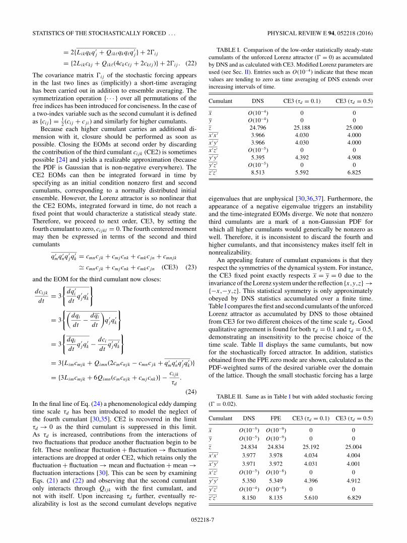
TABLE I. Comparison of the low-order statistically steady-statecumulants of the unforced Lorenz attractor (� = 0) as accumulatedby DNS and as calculated with CE3. Modified Lorenz parameters areused (see Sec. II). Entries such as O(10−4) indicate that these meanvalues are tending to zero as time averaging of DNS extends overincreasing intervals of time.

Cumulant DNS CE3 (τd = 0.1) CE3 (τd = 0.5)

x O(10−4) 0 0y O(10−4) 0 0z 24.796 25.188 25.000x ′x ′ 3.966 4.030 4.000x ′y ′ 3.966 4.030 4.000x ′z′ O(10−5) 0 0y ′y ′ 5.395 4.392 4.908y ′z′ O(10−5) 0 0z′z′ 8.513 5.592 6.825

eigenvalues that are unphysical [30,36,37]. Furthermore, theappearance of a negative eigenvalue triggers an instabilityand the time-integrated EOMs diverge. We note that nonzerothird cumulants are a mark of a non-Gaussian PDF forwhich all higher cumulants would generically be nonzero aswell. Therefore, it is inconsistent to discard the fourth andhigher cumulants, and that inconsistency makes itself felt innonrealizability.

An appealing feature of cumulant expansions is that theyrespect the symmetries of the dynamical system. For instance,the CE3 fixed point exactly respects x = y = 0 due to theinvariance of the Lorenz system under the reflection {x,y,z} →{−x,−y,z}. This statistical symmetry is only approximatelyobeyed by DNS statistics accumulated over a finite time.Table I compares the first and second cumulants of the unforcedLorenz attractor as accumulated by DNS to those obtainedfrom CE3 for two different choices of the time scale τd . Goodqualitative agreement is found for both τd = 0.1 and τd = 0.5,demonstrating an insensitivity to the precise choice of thetime scale. Table II displays the same cumulants, but nowfor the stochastically forced attractor. In addition, statisticsobtained from the FPE zero mode are shown, calculated as thePDF-weighted sums of the desired variable over the domainof the lattice. Though the small stochastic forcing has a large

TABLE II. Same as in Table I but with added stochastic forcing(� = 0.02).

Cumulant DNS FPE CE3 (τd = 0.1) CE3 (τd = 0.5)

x O(10−5) O(10−9) 0 0y O(10−5) O(10−9) 0 0z 24.834 24.834 25.192 25.004

x ′x ′ 3.977 3.978 4.034 4.004

x ′y ′ 3.971 3.972 4.031 4.001

x ′z′ O(10−5) O(10−8) 0 0

y ′y ′ 5.350 5.349 4.396 4.912

y ′z′ O(10−4) O(10−8) 0 0

z′z′ 8.150 8.135 5.610 6.829

052218-7

ALTAN ALLAWALA AND J. B. MARSTON PHYSICAL REVIEW E 94, 052218 (2016)

effect on the fine structure of the PDF, it only changes thecovariances slightly.

V. CONCLUSION

Direct statistical simulation is an attractive alternative tothe accumulation of statistics by direct numerical simula-tion. Transforming the problem of finding the equal-timestatistics of dynamical systems into a problem of sparselinear algebra offers an accurate and elegant alternative totraditional approaches. It would be interesting to employ asparse preconditioner for the large nonsymmetric FPE operatorstudied here, as this should permit even higher resolutions tobe reached, possibly revealing the fine ringlike steps in theLorenz attractor PDF. Galerkin discretizations of the linearoperator may also be interesting to explore.

We also showed that an expansion in equal-time cumulantsclosed at third order is able to reproduce the low-orderstatistics of the attractor, despite its highly nonlinear nature.The cumulant expansion technique is especially good forhigher-dimensional systems due to its speed. Deterministicchaos and stochastic noise are seen to have similar effectson the low-order statistics [11,38] with both contributing tothe variance. By contrast, Fig. 5 shows that the deterministicdynamics of the strange attractor produces high-order statisticsthat stochastic forcing erases.

ACKNOWLEDGMENTS

We are grateful to P. Zucker and D. Venturi for usefuldiscussions. This research was supported in part by NSF GrantsNo. DMR-1306806 and No. CCF-1048701.

[1] R. F. Pawula, Approximation of the linear Boltzmann equationby the Fokker-Planck equation, Phys. Rev. 162, 186 (1967).

[2] L. Pichler, A. Masud, and L. A. Bergman, ComputationalMethods in Stochastic Dynamics (Springer, Berlin, 2013),pp. 69–85.

[3] L. A. Bergman and B. F. Spencer, Jr., Nonlinear StochasticMechanics (Springer, Berlin, 1992), pp. 49–60.

[4] U. von Wagner and W. V. Wedig, On the calculation of stationarysolutions of multi-dimensional Fokker-Planck equations byorthogonal functions, Nonlinear Dyn. 21, 289 (2000).

[5] P. Kumar and S. Narayanan, Solution of Fokker-Planck equationby finite element and finite difference methods for nonlinearsystems, Sadhana 31, 445 (2006).

[6] A. Naess and B. K. Hegstad, Response statistics of van der Poloscillators excited by white noise, Nonlinear Dyn. 5, 287 (1994).

[7] E. N. Lorenz, Deterministic nonperiodic flow, J. Atmos. Sci. 20,130 (1963).

[8] I. Tikhonenkov, A. Vardi, J. R. Anglin, and D. Cohen, MinimalFokker-Planck Theory for the Thermalization of MesoscopicSubsystems, Phys. Rev. Lett. 110, 050401 (2013).

[9] J. Thuburn, Climate sensitivities via a Fokker-Planck adjointapproach, Q. J. R. Meteor. Soc. 131, 73 (2005).

[10] J. Gradisek, S. Siegert, R. Friedrich, and I. Grabec, Analysisof time series from stochastic processes, Phys. Rev. E 62, 3146(2000).

[11] S. Agarwal and J. S. Wettlaufer, Maximal stochastic transportin the Lorenz equations, Phys. Lett. A 380, 142 (2016).

[12] J. M. Heninger, D. Lippolis, and P. Cvitanovic, Neighborhoodsof periodic orbits and the stationary distribution of a noisychaotic system, Phys. Rev. E 92, 062922 (2015).

[13] P. Kumar, S. Narayanan, S. Adhikari, and M. I. Friswell, Fokker-Planck equation analysis of randomly excited nonlinear energyharvester, J. Sound Vib. 333, 2040 (2014).

[14] O. Ma and J. B. Marston, Exact equal time statistics of Orszag-McLaughlin dynamics investigated using the Hopf characteristicfunctional approach, J. Stat. Mech. (2005) P10007.

[15] D. K. Lilly, Numerical simulation of two-dimensional turbu-lence, Phys. Fluids 12, II-240 (1969).

[16] J. Heninger, D. Lippolis, and P. Cvitanovic, Perturbation theoryfor the Fokker-Planck operator in chaos, arXiv:1602.03044.

[17] G. L. G. Sleijpen and H. A. Van der Vorst, A Jacobi-Davidsoniteration method for linear eigenvalue problems, SIAM Rev. 42,267 (2000).

[18] D. R. Fokkema, G. L. G. Sleijpen, and H. A. Van der Vorst,Jacobi-Davidson Style QR and QZ algorithms for the reductionof matrix pencils, SIAM J. Sci. Comput. 20, 94 (1998).

[19] A. B. Finnila, M. A. Gomez, C. Sebenik, C. Stenson, andJ. D. Doll, Quantum annealing: A new method for minimizingmultidimensional functions, Chem. Phys. Lett. 219, 343 (1994).

[20] G. E. Santoro and E. Tosatti, Optimization using quantummechanics: quantum annealing through adiabatic evolution,J. Phys. A 39, R393 (2006).

[21] E. R. Davidson, The iterative calculation of a few of thelowest eigenvalues and corresponding eigenvectors of largereal-symmetric matrices, J. Comput. Phys. 17, 87 (1975).

[22] E. R. Davidson and W. J. Thompson, Monster matrices: Theireigenvalues and eigenvectors, Comput. Phys. 7, 519 (1993).

[23] H. Risken, The Fokker-Planck Equation: Methods of Solutionand Applications (Springer, Berlin, 1984).

[24] J. B. Marston, E. Conover, and T. Schneider, Statistics of anunstable barotropic jet from a cumulant expansion, J. Atmos.Sci. 65, 1955 (2008).

[25] S. M. Tobias, K. Dagon, and J. B. Marston, Astrophysical fluiddynamics via direct statistical simulation, Astrophys. J. 727, 127(2011).

[26] S. M. Tobias and J. B. Marston, Direct Statistical Simulation ofOut-of-Equilibrium Jets, Phys. Rev. Lett. 110, 104502 (2013).

[27] J. B. Parker and J. A. Krommes, Zonal flow as pattern formation,Phys. Plasmas 20, 100703 (2013).

[28] J. B. Parker and J. A. Krommes, Generation of zonal flowsthrough symmetry breaking of statistical homogeneity, New J.Phys. 16, 035006 (2014).

[29] J. Squire and A. Bhattacharjee, Statistical Simulation of theMagnetorotational Dynamo, Phys. Rev. Lett. 114, 085002(2015).

[30] J. B. Marston, W. Qi, and S. M. Tobias, Direct statisticalsimulation of a jet, arXiv:1412.0381.

[31] F. A. Chaalal, T. Schneider, B. Meyer, and J. B. Marston,Cumulant expansions for atmospheric flows, New J. Phys. 18,025019 (2016).

052218-8

STATISTICS OF THE STOCHASTICALLY FORCED . . . PHYSICAL REVIEW E 94, 052218 (2016)

[32] N. A. Bakas and P. J. Ioannou, Emergence of Large ScaleStructure in Barotropic β-plane turbulence, Phys. Rev. Lett. 110,224501 (2013).

[33] N. A. Bakas, N. C. Constantinou, and P. J. Ioannou, S3T stabilityof the homogeneous state of barotropic beta-plane turbulence,J. Atmos. Sci. 72, 1689 (2015).

[34] U. Frisch, Turbulence: The Legacy of A. N. Kolmogorov(Cambridge University Press, Cambridge, 1995).

[35] S. A. Orszag, Lectures on the statistical theory of turbulence,in Fluid Dynamics, edited by R. Balian and J.-L. Peube,

Proceedings of the Les Houches Summer School of TheoreticalPhysics (Gordon and Breach, London, 1977). pp. 235–374.

[36] R. H. Kraichnan, Realizability inequalities and closedmoment equations, Ann. NY Acad. Sci. 357, 37(1980).

[37] P. Hanggi and P. Talkner, A remark on truncationschemes of cumulant hierarchies, J. Stat. Phys. 22, 65(1980).

[38] E. Knobloch, On the statistical dynamics of the Lorenz model,J. Stat. Phys. 20, 695 (1979).

052218-9