1

Set Predicates in SQL: Enabling Set-LevelComparisons for Dynamically Formed Groups

Chengkai Li, Member, IEEE, Bin He, Ning Yan, Muhammad Assad Safiullah

Abstract —In data warehousing and OLAP applications, scalar-level predicates in SQL become increasingly inadequate to supporta class of operations that require set-level comparison semantics, i.e., comparing a group of tuples with multiple values. Currently,complex SQL queries composed by scalar-level operations are often formed to obtain even very simple set-level semantics. Suchqueries are not only difficult to write but also challenging for a database engine to optimize, thus can result in costly evaluation. Thispaper proposes to augment SQL with set predicate, to bring out otherwise obscured set-level semantics. We studied two approachesto processing set predicates– an aggregate function-based approach and a bitmap index-based approach. Moreover, we designeda histogram-based probabilistic method of set predicate selectivity estimation, for optimizing queries with multiple predicates. Theexperiments verified its accuracy and effectiveness in optimizing queries.

Index Terms —Set Predicates, Grouping, Data Warehousing, OLAP, Querying Processing and Optimization

✦

1 INTRODUCTION

With data warehousing and OLAP applications becomingmore sophisticated, there is a high demand of querying datawith the semantics ofset-level comparisons. For instance, acompany may search its resume database for job candidateswith a set of mandatory skills. Here the skills of each candi-date, as a set of values, are compared against the mandatoryskills. Such sets are often dynamically formed. For example,suppose a tableResume Skills (id, skill) connects skills tojob candidates. A GROUP BY clause dynamically groups thetuples in it byid, with the values on attributeskill in each groupforming a set. The problem is that the current GROUP BYclause can only do scalar value comparison by an accompany-ing HAVING clause. For instance, aggregate functions SUM/COUNT/ AVG/ MAX produce a single numeric value whichis compared to a literal or another single aggregate value.

Observing the demand for complex and dynamic set-levelcomparisons in databases, we propose a concept ofset predi-cate. Below are several example queries with set predicates.

Example 1: To find those candidates with skills “Java” and“Web services”, our query can be as follows. After grouping,a dynamic set of values on attributeskill is formed foreach uniqueid, and groups whose corresponding SET(skill)contains both “Java” and “Web services” are returned.

SELECT id FROM Resume_Skills GROUP BY idHAVING SET(skill) CONTAIN {’Java’,’Web services’}

• C. Li and N. Yan are with the Department of Computer Science andEngineering, The University of Texas at Arlington, Arlington, TX 76019.E-mail: cli@uta.edu, ning.yan@mavs.uta.edu

• B. He is with IBM Almaden Research Center, San Jose, CA 95120.E-mail:binhe@us.ibm.com

• M. A. Safiullah is with Microsoft, Seattle, WA. E-mail:assad.safiullah@live.com. The work was done while the author wasa student at UT-Arlington.

Example 2: In business decision making, an executive maywant to find the departments whose monthly average ratingsfor customer service in 2009 have always been poor (assumingratings are from 1 to 5). Suppose the table schema isRat-ings(department, avg rating, month, year). The followingquery uses CONTAINED BY for the set-level condition.

SELECT department FROM Ratings WHERE year=2009GROUP BY departmentHAVING SET(avg_rating) CONTAINED BY {1,2}

Example 3: Set predicates can be defined across multipleattributes. Consider an online advertisement example. Supposethe table schema isSite Statistics(website, advertiser, C-TR). A marketing strategist uses the following query to findWebsites that publish ads for ING with more than 1% and lessthan 2% click-through rate (CTR) and do not publish ads forHSBC yet:

SELECT website FROM Site_StatisticsGROUP BY website HAVING

SET(advertiser,CTR) CONTAIN {(’ING’,[0.01,0.02])}AND NOT (SET(advertiser) CONTAIN {’HSBC’})

In this example, the first set predicate involves two attributesand the second set predicate uses the negation of CONTAIN.Note that we use[0.01,0.02] to represent a range-basedcondition 0.01≤CTR≤0.02.

The semantics of set-level comparisons in many cases canbe expressed using current SQL syntax without the proposedextension. However, resulting queries would be more complexthan necessary. One consequence is that complex queriesare difficult for users to formulate. More importantly, suchcomplex queries are difficult for DBMS to optimize, leadingto unnecessarily costly evaluation. The resulting query planscould involve multiple subqueries with grouping and set op-erations. On the contrary, the proposed concise syntax of setpredicates enables direct expression of set-level comparisonsin SQL, which not only makes query formulation simple butalso facilitates efficient support of such queries. We developedtwo approaches to process set predicates:

2

Aggregate function-based approach: This approach process-es set predicates in a way similar to processing conventionalaggregate functions. Given a query with set predicates, insteadof decomposing the query into multiple subqueries, this ap-proach only needs one pass of table scan.

Bitmap index-based approach: This approach processes setpredicates by using bitmap indices on individual attributes. Itis efficient because it can focus on only the tuples from thosegroups that satisfy query conditions and only the bitmaps forrelevant columns. State-of-the-art bitmap compression meth-ods [33], [2], [16] and encoding strategies [5], [34], [23] havemade it affordable to build bitmap index on many attributes.This index structure is also applicable on many differenttypes of attributes. The bitmap index-based approach processesgeneral queries (with joins, selections, multi-attributegroup-ing and multiple set predicates) by utilizing single-attributeindices. Hence it does not require pre-computed index for joinresults or combination of attributes.

We further developed an optimization strategy to handlequeries with multiple set predicates connected by logic op-erations (AND, OR, NOT). A useful optimization rule isto prune unnecessary set predicates during query evaluation.Given a query withn conjunctive set predicates, the predicatescan be sequentially evaluated. If no group qualifies aftermpredicates are processed, we can terminate query evaluationwithout processing the remaining predicates. The number of“necessary” predicates before we can stop,m, depends onthe evaluation order of predicates. We designed a method toselect a good order of predicate evaluation, i.e, an order thatresults in smallm, thus cheap evaluation cost. Our idea is toevaluate conjunctive (disjunctive) predicates in the ascending(descending) order of their selectivities, where the selectivityof a predicate is its number of qualified groups. We designeda probabilistic approach to estimating set predicate selectivityby database histograms.

In summary, this paper makes the following contributions:

• We proposed to extend SQL with set predicates for animportant class of analytical queries, which otherwise wouldbe difficult to write and optimize (Section 3).• We designed two query evaluation approaches for setpredicates, including an aggregate function-based approach(Section 5) and a bitmap index-based approach (Section 6).• We developed a histogram-based probabilistic method toestimate the selectivity of a set predicate, for optimizingqueries with multiple predicates (Section 8).• We conducted extensive experiments to evaluate proposedapproaches over both real and synthetic data (Section 9).

2 RELATED WORK

Set-valued attributes provide a concise and natural way tomodel complex data concepts such as sets [24], [29]. ManyDBMSs nowadays support the definition of attributes involvinga set of values, e.g.,nested tablein Oracle andSETdata typein MySQL. For example, the “skill” attribute in Example 1 canbe defined as a set data type. Set operations can be nativelysupported on such attributes. Query processing on set-valuedattributes and set containment joins have been extensively

studied [14], [27], [18], [19]. Although set-valued attributestogether with set containment joins can support set-levelcomparisons, set predicates have several critical advantages:

(1) Unlike set-valued attributes, which bring hassles inredesigning database storage for the special set data type,set predicates require no change in data representation andstorage, and thus can be incorporated into standard RDBMS.

(2) In real-world applications, groups and correspondingsets are often dynamically formed according to query needs.For instance, in Example 2, the monthly ratings of eachdepartment form a set. In a different query, sets may beformed by ratings of individual employees. With set predi-cates, users can dynamically form set-level comparisons withno limitation caused by database schema. On the contrary,set-valued attributes cannot support dynamic set formationbecause they are pre-defined at schema definition phase andset-level comparisons can only be issued on such attributes.

(3) Set predicates allow cross-attribute set-level comparison.For instance, sets are defined overadvertiser and CTRtogether in Example 3. On the contrary, a set-valued attributecan only be defined on a single attribute in many imple-mentations, thus cannot capture cross-attribute associations.Implementations such as nested table in Oracle allow setsover multiple attributes but do not easily support set-levelcomparisons on such attributes.

Set predicate is also related to universal quantification andrelational division [12], which are powerful for analyzingmany-to-many relationships. An example universal quantifica-tion query is to find the students that have taken all computerscience courses required to graduate. It is a special type ofsetpredicates with CONTAIN operator over all the values of anattribute in a table, e.g.,Courses. By contrast, the proposedset predicates allow sets to be dynamically formed throughGROUP BY and support CONTAINED BY and EQUAL, inaddition to CONTAIN.

The SEQUEL 2 language (an extension of the originalSEQUEL) for SYSTEM R proposed a special SET function,for comparing a set of attribute values with the result ofa subquery [4]. The proposed comparison operators includeCONTAINS, =, and their negations. Furthermore, these oper-ators can be used in comparing the results of two subqueries.The proposal was brief, by several example queries. The SETfunction is only on one attribute and does not allow range-based values or bag semantics. No suggestion for implementa-tion techniques was made. The SET function and CONTAINSoperator were later dropped from the SQL language, possiblybecause of the difficulty in implementing it efficiently [11].

In [8], [9], [7], [10] the concept ofgrouping variableandassociated setwas introduced as an SQL extension to allowcomparisons of multiple aggregates over the same groupingcondition. That line of work only considered regular aggre-gates such as SUM and COUNT. Combining the concepts ofset predicate and grouping variable can allow simpler syntaxfor complex queries. We provide more detailed discussions ofthis in the supplemental materials to this paper.

This paper focuses on relational data model and architecture.Some data analytics systems today are built on top of massiveparallel computing architecture. The query languages for such

3

semester student course grade

Fall09 Mary CS101 4

Fall09 Mary CS102 2

Fall09 Tom CS102 4

Spring10 Tom CS103 3

Fall09 John CS101 4

Fall09 John CS102 4

Spring10 John CS103 3

Table: SC

Fig. 1. A classic student and course example.

systems (e.g., Pig Latin [21], Dremel [20], Jaql [1]) deal withcomplex data models such as set-valued attributes, maps, andnested data. Due to the fundamental architectural difference,supporting set predicates in such systems, although a veryinteresting future topic, is beyond the scope of this paper.

3 SET PREDICATES

We extend SQL syntax to support set predicates. Since a setpredicate compares a group of tuples to a set of values, it fitswell into GROUP BY and HAVING clauses. Specifically in aHAVING clause there is a Boolean expression over multipleregular aggregate predicates and set predicates, connected bylogic operators ANDs, ORs, and NOTs. The syntax of a setpredicate is:

SET(v1, ..., vm)CONTAIN | CONTAINED BY | EQUAL{(v11 , ..., v1m), ..., (vn1 , ..., vnm)},

wherevji ∈ Dom(vi), i.e., eachvji is a literal value (integer,floating point number, etc.) in the domain of attributevi.Succinctly we denote a set predicate by (v1, ..., vm) op {(v11,..., v1m), ..., (vn1 , ..., vnm)}, where op can be⊇, ⊆, and =,corresponding to set operator CONTAIN, CONTAINED BY,and EQUAL, respectively.

The syntax can be extended to allow set-level comparisonwith not only literal values, but also another dynamicallyformed group or the result of a subquery. We focus on literalvalues in the following sections and discuss such extensioninthe supplemental materials.

We further use relational algebra to concisely representqueries with set predicates. Given a relationR, grouping andaggregation are represented by the following operator:

γG,AC(R)

where G is a set of grouping attributes,A is a set ofaggregates (e.g., COUNT(*)), andC is a Boolean expres-sion over set predicates and conditions on aggregates (e.g.,AVG(grade)>3). The aggregates inA andC may overlap.

We now provide example queries over the classic student-course table (Figure 1). We use full SQL for the first query aswe did in Section 1. For remaining queries, we will show eitheronly set predicates or succinct relational algebra expressions.

The following Q1: γstudent course ⊇{‘CS101’,‘CS102’}(SC) i-dentifies the students who took both CS101 and CS102.1 Theresults are Mary and John. The keyword CONTAIN represents

1. To be rigorous, it should be (course) ⊇ {(‘CS101’), (‘CS102’)}, basedon the aforementioned syntax.

a superset relationship,i.e., the set variable SET(course) is asuperset of{‘CS101’, ‘CS102’}.

Q1: SELECT student FROM SC GROUP BY studentHAVING SET(course) CONTAIN {’CS101’, ’CS102’}

A query can include WHERE clause and regular aggregatefunctions in HAVING. In Q2: γstudent,COUNT (∗) course ⊇

{‘CS101’, ‘CS102’}∧

AVG(grade) > 3.5 (σsemester= ′Fall09′ (SC)), welook for those students that had average grade higher than 3.5in FALL09 and took both CS101 and CS102 in that semester.It also returns the number of courses they took in that semester.

We use CONTAINED BY for the reverse of CONTAIN,i.e., the subset relationship. Query Q3:γstudent grade⊆{4,3}(SC)

selects all the students whose grades are never below 3. Theresults are Tom and John.

To select the students that have only taken CS101 and C-S102, we use EQUAL to represent the equal relationship in settheory. The query is Q4:γstudent course ={‘CS101’,‘CS102’}(SC).Its result contains only Mary.

In above queries we assumed set predicates follow setsemantics. Therefore John’s grades,{4,4,3}, are subsumedby {4,3}. The syntax also allows bag semantics for setpredicates, whereγstudent course ⊇{‘CS101’,‘CS101’,‘CS102’}(SC)

finds students who took CS101 twice and CS102 once, andγstudent grade ⊆{4,4,3}(SC) selects students who have obtainedgrade 4 in at most 2 courses and grade 3 in at most 1 courseand have no other grades in record.

Note that the set/bag semantics of set predicates are orthog-onal to the set/bag semantics of regular SQL constructs. If setsemantics is applied for a set predicate, only distinct valueson the set predicate attribute from the tuples in a group areused in determining if the group satisfies the set predicate.However, if (the default) bag semantics is applied for regularSQL operations, all the tuples in the group are included incalculating aggregates. For example,γstudent,AV G(grade) grade

⊇{4,4,3}(SC) calculates GPA for students with at least two 4sand one 3, and all their grades are included in GPA calculation.

For simplicity of presentation, in the following sections wefocus on the simplest query–γg,⊕a v op {v1, ...,vn}(R), i.e., aquery with one grouping attribute (g), one aggregate for output(⊕a), and one set predicate defined by a set operatorop (⊇,⊆, or =) over a single attribute (v). Moreover set semanticsis assumed for set predicates. In Section 7 we discuss thesyntax of expressing more general queries and the methods ofprocessing general queries.

4 DRAWBACKS OF SET-LEVEL COMPARISONSBY REGULAR SQLWithout the proposed set predicate, we fall back to currentSQL syntax in expressing set-level comparisons. Complexqueries containing scalar-level operations are often formed toobtain even very simple set-level semantics. Such complexqueries are difficult for users to formulate. A more severeconsequence is that set-level semantics becomes obscure.Hence a DBMS may choose unnecessarily costly evaluationplans for such queries.

The semantics of set predicates can often be expressed bystandard SQL queries. In fact, there can be multiple ways in

4

SELECT R.g, sum(a)FROM R,

Seq Scan

39.063 ms

368.190 ms

FROM R,( SELECT gFROM REXCEPT( SELECT g FROM RWHERE v <> 1 AND v <> 2 AND v <> 3)

) AS TMPWHERE R.g = TMP.g

Seq Scan

R

WHERE R.g = TMP.gGROUP BY R.g

Hash Join

Hash Aggregate

402.067 ms

402.468 ms

Seq Scan

Except

Project &

Sort on g

Append

Seq Scan

R

39.063 ms

161.989 ms

328.102 ms

368.190 ms 14.791 ms

Filter38.950 ms

Seq Scan

Seq Scan

R38.950 ms

Filter

v<> 1 && v<>2 && v<>3

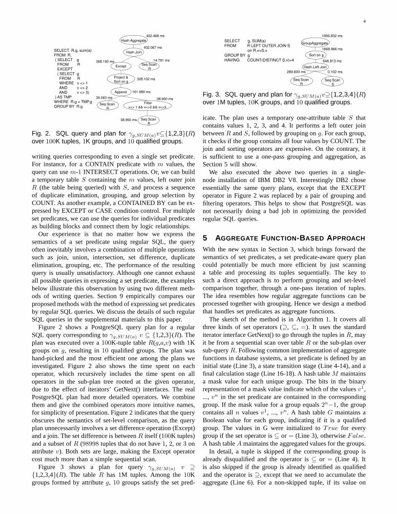
Fig. 2. SQL query and plan for γg,SUM(a)v⊆{1,2,3}(R)over 100K tuples, 1K groups, and 10 qualified groups.

writing queries corresponding to even a single set predicate.For instance, for a CONTAIN predicate withm values, thequery can usem-1 INTERSECT operations. Or, we can builda temporary tableS containing them values, left outer joinR (the table being queried) withS, and process a sequenceof duplicate elimination, grouping, and group selection byCOUNT. As another example, a CONTAINED BY can be ex-pressed by EXCEPT or CASE condition control. For multipleset predicates, we can use the queries for individual predicatesas building blocks and connect them by logic relationships.

Our experience is that no matter how we express thesemantics of a set predicate using regular SQL, the queryoften inevitably involves a combination of multiple operationssuch as join, union, intersection, set difference, duplicateelimination, grouping, etc. The performance of the resultingquery is usually unsatisfactory. Although one cannot exhaustall possible queries in expressing a set predicate, the examplesbelow illustrate this observation by using two different meth-ods of writing queries. Section 9 empirically compares ourproposed methods with the method of expressing set predicatesby regular SQL queries. We discuss the details of such regularSQL queries in the supplemental materials to this paper.

Figure 2 shows a PostgreSQL query plan for a regularSQL query corresponding toγg,SUM(a) v ⊆ {1,2,3}(R). Theplan was executed over a100K-tuple tableR(g,a,v) with 1Kgroups ong, resulting in10 qualified groups. The plan washand-picked and the most efficient one among the plans weinvestigated. Figure 2 also shows the time spent on eachoperator, which recursively includes the time spent on alloperators in the sub-plan tree rooted at the given operator,due to the effect of iterators’ GetNext() interfaces. The realPostgreSQL plan had more detailed operators. We combinethem and give the combined operators more intuitive names,for simplicity of presentation. Figure 2 indicates that thequeryobscures the semantics of set-level comparison, as the queryplan unnecessarily involves a set difference operation (Except)and a join. The set difference is betweenR itself (100K tuples)and a subset ofR (98998 tuples that do not have1, 2, or 3 onattributev). Both sets are large, making the Except operatorcost much more than a simple sequential scan.

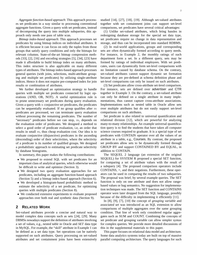
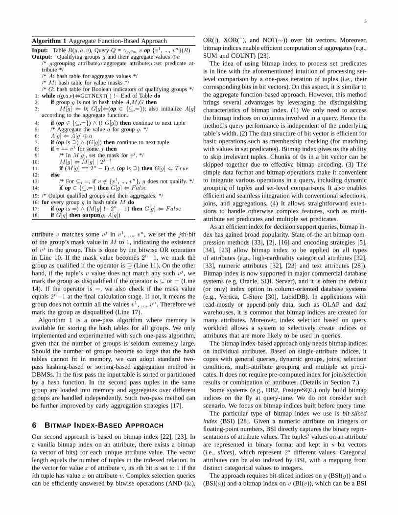
Figure 3 shows a plan for queryγg,SUM(a) v ⊇{1,2,3,4}(R). The tableR has 1M tuples. Among the10Kgroups formed by attributeg, 10 groups satisfy the set pred-

SELECT g, SUM(a)FROM R LEFT OUTER JOIN S

on R.v=S.vGROUP BY gHAVING COUNT(DISTINCT S.v)=4HAVING COUNT(DISTINCT S.v)=4

289.600 ms

FROM R LEFT OUTER JOIN S

HAVING COUNT(DISTINCT S.v)=4

Sort on g

GroupAggregate

646.813 ms

1669.966 ms

1956.832 ms

HAVING COUNT(DISTINCT S.v)=4

Seq Scan

RSeq Scan

S

Hash Left Join

0.102 ms289.600 ms

646.813 ms

Fig. 3. SQL query and plan for γg,SUM(a)v⊇{1,2,3,4}(R)over 1M tuples, 10K groups, and 10 qualified groups.

icate. The plan uses a temporary one-attribute tableS thatcontains values 1, 2, 3, and 4. It performs a left outer joinbetweenR andS, followed by grouping ong. For each group,it checks if the group contains all four values by COUNT. Thejoin and sorting operators are expensive. On the contrary, itis sufficient to use a one-pass grouping and aggregation, asSection 5 will show.

We also executed the above two queries in a single-node installation of IBM DB2 V8. Interestingly DB2 choseessentially the same query plans, except that the EXCEPToperator in Figure 2 was replaced by a pair of grouping andfiltering operators. This helps to show that PostgreSQL wasnot necessarily doing a bad job in optimizing the providedregular SQL queries.

5 AGGREGATE FUNCTION-BASED APPROACH

With the new syntax in Section 3, which brings forward thesemantics of set predicates, a set predicate-aware query plancould potentially be much more efficient by just scanninga table and processing its tuples sequentially. The key tosuch a direct approach is to perform grouping and set-levelcomparison together, through a one-pass iteration of tuples.The idea resembles how regular aggregate functions can beprocessed together with grouping. Hence we design a methodthat handles set predicates as aggregate functions.

The sketch of the method is in Algorithm 1. It covers allthree kinds of set operators (⊇, ⊆, =). It uses the standarditerator interface GetNext() to go through the tuples inR, mayit be from a sequential scan over tableR or the sub-plan oversub-queryR. Following common implementation of aggregatefunctions in database systems, a set predicate is defined by aninitial state (Line 3), a state transition stage (Line 4-14), and afinal calculation stage (Line 16-18). A hash tableM maintainsa mask value for each unique group. The bits in the binaryrepresentation of a mask value indicate which of the valuesv1,..., vn in the set predicate are contained in the correspondinggroup. If the mask value for a group equals2n−1, the groupcontains alln valuesv1, ..., vn. A hash tableG maintains aBoolean value for each group, indicating if it is a qualifiedgroup. The values in G were initialized toTrue for everygroup if the set operator is⊆ or = (Line 3), otherwiseFalse.A hash tableA maintains the aggregated values for the groups.

In detail, a tuple is skipped if the corresponding group isalready disqualified and the operator is⊆ or = (Line 4). Itis also skipped if the group is already identified as qualifiedand the operator is⊇, except that we need to accumulate theaggregate (Line 6). For a non-skipped tuple, if its value on

5

Algorithm 1 Aggregate Function-Based Approach

Input: TableR(g, a, v), QueryQ = γg,⊕a v op {v1, ..., vn}(R)Output: Qualifying groupsg and their aggregate values⊕a

/* g:grouping attribute;a:aggregate attribute;v:set predicate at-tribute *//* A: hash table for aggregate values *//* M : hash table for value masks *//* G: hash table for Boolean indicators of qualifying groups */

1: while r(g,a,v)⇐GETNEXT( ) != End of Tabledo2: if groupg is not in hash tableA,M ,G then3: M [g] ⇐ 0; G[g]⇐(op ∈ {⊆,=}); also initialize A[g]

according to the aggregate function.4: if (op ∈ {⊆,=}) ∧ (! G[g]) then continue to next tuple5: /* Aggregate the valuea for groupg. */6: A[g] ⇐ A[g]⊕ a7: if (op is ⊇) ∧ (G[g]) then continue to next tuple8: if v == vj for somej then9: /* In M [g], set the mask forvj . */

10: M [g] ⇐ M [g] | 2j−1

11: if (M [g] == 2n − 1) ∧ (op is ⊇) then G[g] ⇐ True12: else13: /* For ⊆, =, if v /∈ {v1, ..., vn}, g does not qualify. */14: if op ∈ {⊆,=} then G[g] ⇐ False

15: /* Output qualified groups and their aggregates. */16: for every groupg in hash tableM do17: if (op is =) ∧ (M [g] != 2n − 1) then G[g] ⇐ False18: if G[g] then output(g, A[g])

attributev matches somevj in v1, ..., vn, we set thejth-bitof the group’s mask value inM to 1, indicating the existenceof vj in the group. This is done by the bitwise OR operationin Line 10. If the mask value becomes2n−1, we mark thegroup as qualified if the operator is⊇ (Line 11). On the otherhand, if the tuple’sv value does not match any suchvj , wemark the group as disqualified if the operator is⊆ or = (Line14). If the operator is=, we also check if the mask valueequals2n−1 at the final calculation stage. If not, it means thegroup does not contain all the valuesv1, ..., vn. Therefore wemark the group as disqualified (Line 17).

Algorithm 1 is a one-pass algorithm where memory isavailable for storing the hash tables for all groups. We onlyimplemented and experimented with such one-pass algorithm,given that the number of groups is seldom extremely large.Should the number of groups become so large that the hashtables cannot fit in memory, we can adopt standard two-pass hashing-based or sorting-based aggregation method inDBMSs. In the first pass the input table is sorted or partitionedby a hash function. In the second pass tuples in the samegroup are loaded into memory and aggregates over differentgroups are handled independently. Such two-pass method canbe further improved by early aggregation strategies [17].

6 B ITMAP INDEX-BASED APPROACH

Our second approach is based on bitmap index [22], [23]. Ina vanilla bitmap index on an attribute, there exists a bitmap(a vector of bits) for each unique attribute value. The vectorlength equals the number of tuples in the indexed relation. Inthe vector for valuex of attributev, its ith bit is set to1 if theith tuple has valuex on attributev. Complex selection queriescan be efficiently answered by bitwise operations (AND (&),

OR(|), XOR( ), and NOT(∼)) over bit vectors. Moreover,bitmap indices enable efficient computation of aggregates (e.g.,SUM and COUNT) [23].

The idea of using bitmap index to process set predicatesis in line with the aforementioned intuition of processing set-level comparison by a one-pass iteration of tuples (i.e., theircorresponding bits in bit vectors). On this aspect, it is similar tothe aggregate function-based approach. However, this methodbrings several advantages by leveraging the distinguishingcharacteristics of bitmap index. (1) We only need to accessthe bitmap indices on columns involved in a query. Hence themethod’s query performance is independent of the underlyingtable’s width. (2) The data structure of bit vector is efficient forbasic operations such as membership checking (for matchingwith values in set predicates). Bitmap index gives us the abilityto skip irrelevant tuples. Chunks of 0s in a bit vector can beskipped together due to effective bitmap encoding. (3) Thesimple data format and bitmap operations make it convenientto integrate various operations in a query, including dynamicgrouping of tuples and set-level comparisons. It also enablesefficient and seamless integration with conventional selections,joins, and aggregations. (4) It allows straightforward exten-sions to handle otherwise complex features, such as multi-attribute set predicates and multiple set predicates.

As an efficient index for decision support queries, bitmap in-dex has gained broad popularity. State-of-the-art bitmap com-pression methods [33], [2], [16] and encoding strategies [5],[34], [23] allow bitmap index to be applied on all typesof attributes (e.g., high-cardinality categorical attributes [32],[33], numeric attributes [32], [23] and text attributes [28]).Bitmap index is now supported in major commercial databasesystems (e.g, Oracle, SQL Server), and it is often the default(or only) index option in column-oriented database systems(e.g., Vertica, C-Store [30], LucidDB). In applications withread-mostly or append-only data, such as OLAP and datawarehouses, it is common that bitmap indices are created formany attributes. Moreover, index selection based on queryworkload allows a system to selectively create indices onattributes that are more likely to be used in queries.

The bitmap index-based approach only needs bitmap indiceson individual attributes. Based on single-attribute indices, itcopes with general queries, dynamic groups, joins, selectionconditions, multi-attribute grouping and multiple set predi-cates. It does not require pre-computed index for join/selectionresults or combination of attributes. (Details in Section 7.)

Some systems (e.g., DB2, PostgreSQL) only build bitmapindices on the fly at query-time. We do not consider suchscenario. We focus on bitmap indices built before query time.

The particular type of bitmap index we use isbit-slicedindex (BSI) [28]. Given a numeric attribute on integers orfloating-point numbers, BSI directly captures the binary repre-sentations of attribute values. The tuples’ values on an attributeare represented in binary format and kept ins bit vectors(i.e., slices), which represent2s different values. Categorialattributes can be also indexed by BSI, with a mapping fromdistinct categorical values to integers.

The approach requires bit-sliced indices ong (BSI(g)) anda(BSI(a)) and a bitmap index onv (BI(v)), which can be a BSI

6

Algorithm 2 Bitmap Index-Based ApproachInput: TableR(g, a, v) with t tuples;

QueryQ = γg,⊕a v op {v1, ..., vn}(R);bit-sliced index BSI(g), BSI(a), and bitmap index BI(v).

Output: Qualified groupsg and their aggregate values⊕a/* gID: array of sizet, storing the group ID of each tuple *//* A: hash table for aggregate values *//* M : hash table for value masks *//* G: hash table for Boolean indicators of qualified groups *//* Step 1. get the vector for eachvj in the predicate */

1: for eachvj do2: vecvj ⇐ QUERYBI (BI(v), vj )

/* Step 2. get the group ID for each tuple */3: Initialize gID to all zero4: for each bit sliceBi in BSI(g), i from 0 to s-1 do5: for each set bitbk in bit vectorBi do6: gID[k] ⇐ gID[k] + 2i

7: for eachk from 0 to t-1 do8: if groupgID[k] is not in hash tableA,M ,G then9: M [gID[k]]⇐0; G[gID[k]] ⇐ False; also initialize

A[gID[k]] according to the aggregate function./* Step 3. find qualified groups */

10: if op ∈ {⊇, =} then11: for each bit vectorvecvj do12: for each set bitbk in vecvj do13: M [gID[k]] ⇐ M [gID[k]] | 2j−1

14: for each groupg in hash tableM do15: G[g] ⇐ (M [g] == 2n − 1)16: if op ∈ {⊆, =} then17: for each set bitbk in ∼(vecv1 | ... | vecvn ) do18: G[gID[k]] ⇐ False

/* Step 4. aggregate the values ofa for qualified groups */19: for eachk from 0 to t-1 do20: if G[gID[k]] then21: agg ⇐ 022: for each sliceBi in BSI(a) do23: if bk is set in bit vectorBi then agg ⇐ agg + 2i

24: A[gID[k]] ⇐ A[gID[k]]⊕ agg

25: for every groupg in hash tableM do26: if G[g] then output (g, A[g])

or other type of bitmap index. Note that the algorithm belowwill also work if we have other types of bitmap indices onganda, with modifications that we omit. The advantage of BSIis that it indexes high-cardinality attributes with small numberof bit vectors, thus improves query performance if groupingor aggregation is on such high-cardinality attributes.

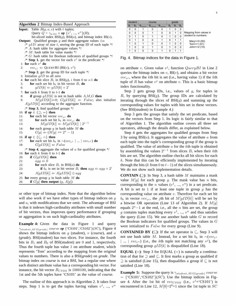
Example 4: Given the data in Figure 1 and queryγstudent,AV G(grade) course op {‘CS101’,‘CS102’}(SC), Figure 4shows the bitmap indices ong (student), v (course), and a(grade). BSI(student) has two slices. For instance, the fourthbits in B1 andB0 of BSI(student) are 0 and 1, respectively.Thus the fourth tuple has value1 on attributestudent, whichrepresents ‘Tom’ according to the mapping from the originalvalues to numbers. There is also a BSI(grade) on grade. Thebitmap index oncourseis not a BSI, but a regular one whereeach distinct attribute value has a corresponding bit vector. Forinstance, the bit vectorBCS101 is 1000100, indicating that the1st and the5th tuples have ‘CS101’ as the value ofcourse.

The outline of this approach is in Algorithm 2. It takes foursteps. Step 1 is to get the tuples having valuesv1, ..., vn

Mapping from values in student to numbers:

Mary=>0 (00)Tom=>1 (01)John=>2 (10)

student course grade

B1 B0 BCS101 BCS102 BCS103 B2 B1 B0

0 0 1 0 0 1 0 0

0 0 0 1 0 0 1 0

0 1 0 1 0 1 0 0

0 1 0 0 1 0 1 1

1 0 1 0 0 1 0 0

1 0 0 1 0 1 0 0

1 0 0 0 1 0 1 1

Fig. 4. Bitmap indices for the data in Figure 1.

on attributev. Given valuevj , functionQueryBI in Line 2queries the bitmap index onv, BI(v), and obtains a bit vectorvecvj , where thekth bit is set (i.e., having value1) if the kthtuple ofR has valuevj on attributev. This is a basic bitmapindex functionality.

Step 2 gets group IDs, i.e., values ofg, for tuples inR, by querying BSI(g). The group IDs are calculated byiterating through the slices of BSI(g) and summing up thecorresponding values for tuples with bits set in these vectors.(See BSI(student) in Example 4.)

Step 3 gets the groups that satisfy the set predicate, basedon the vectors from Step 1. Its logic is fairly similar to thatof Algorithm 1. The algorithm outline covers all three setoperators, although the details differ, as explained below.

Step 4 gets the aggregates for qualified groups from Step3 by using BSI(a). It aggregates the value of attributea fromeach tuple into the tuple’s corresponding group if the groupisqualified. The value of attributea for thekth tuple is obtainedby assembling the values2i−1 from slicesBi when theirkthbits are set. The algorithm outline checks all bit slices foreachk. Note that this can be efficiently implemented by iteratingthrough the bits (k from 0 to t−1) of the slices simultaneously.We do not show such implementation details.

CONTAIN (⊇): In Step 3, a hash tableM maintains a maskvalue M [g] for each groupg. The mask value hasn bits,corresponding to then values (v1, ..., vn) in a set predicate.A bit is set to 1 if at least one tuple in groupg has thecorresponding value on attributev. Therefore for each set bitbk in vector vecvj , the jth bit of M [gID[k]] will be set bya bitwise OR operation (Line 13 of Algorithm 2). IfM [g]equals2n−1 at the end, i.e., all then bits are set, the groupg contains tuples matching everyv1, ..., vn and thus satisfiesthe query (Line 15). We use another hash tableG to recordthe Boolean indicators for qualified groups. The values inGwere initialized toFalse for every group (Line 9).

CONTAINED BY (⊆): If the set operator is⊆, Step 3 willnot use hash tableM . Instead, for a set bitbk in ∼(vecv1

| ... | vecvn ) (i.e., thekth tuple not matching anyvj), thecorresponding groupgID[k] is disqualified (Line 18).

EQUAL (=): Step 3 for EQUAL (=) is naturally a combina-tion of that for⊇ and⊆. It first marks a group as qualified if⊇ is satisfied (Line 15), then disqualifies a group if⊆ is notsatisfied (Line 18).

Example 5: Suppose the query isγstudent,AV G(grade) course= {‘CS101’,‘CS102’}(SC). Use the bitmap indices in Fig-ure 4. After the 1st bit ofvecCS101 (i.e., v1=‘CS101’) isencountered in Line 12,M [0]=20=1 since the 1st tuple inSC

7

belongs to group0 (Mary). After the 2nd bit ofvecCS102

(the 1st set bit) is encountered,M [0]=1|21=3. ThereforeG[0]becomesTrue. Similarly G[2] (for John) becomesTrueafter the 6th bit ofvecCS102 is encountered. However, since∼(vecCS101 | vecCS102) is 0001001, G[2] becomesFalseafter the last bit of0001001 is encountered in Line 17 (i.e.,John has an extra course ‘CS103’).

7 GENERAL SET PREDICATE QUERIES

Our discussion so far has focused on simple queries thathave one grouping attribute, one aggregate for output, andone single-attribute set predicate, under set semantics ofsetpredicates. As introduced in Section 3, more general query isdenoted byγG,AC(R), whereG is a set of grouping attributes(appear in GROUP BY clause),A is a set of regular aggregatesfor output (appear in SELECT), andC is a Boolean expres-sion over set predicates and conditions on regular aggregates(appear in HAVING). In this section we discuss how to extendour algorithms for general queries.

(A) Multi-Attribute Grouping: Given a query with multiplegrouping attributes,γg1,...gl,A C(R), we can treat the groupingattributes as a single combined attributeg. That is, the con-catenation of the bit slices of BSI(g1), ..., BSI(gl) becomesthe bit slices of BSI(g). For example, given Figure 4, ifthe grouping condition isGROUP BY student,grade, theBSI of the conceptual combined attributeg has 5 slices,which areB1(student), B0(student), B2(grade), B1(grade),andB0(grade). Thus the binary value of the combined groupg of the first tuple is00100.

(B) Multi-Attribute Set Predicate: The query syntaxalso allows comparing sets defined on multiple attributes,e.g., SET(course, grade) CONTAIN {(’CS101’,4),

(’CS102’,2)} finds all the students who received grade 4in CS101 and 2 in CS102. In general, for a query with aset predicate defined on multiple attributes,γG,A (v1, ..., vm)op {(v11, ..., v1m), ..., (vn1 , ..., vnm)}(R), we replace Step 1 ofAlgorithm 2 as follows. We first obtain vectorsvec

vj1

, ...,vec

vjm

by querying BI(v1), ..., BI(vm). Then their intersection(bitwise AND), vecvj = vec

vj1

& ... & vecvjm

, gives us the

tuples that match the multi-attribute value (vj1, ..., vjm).

(C) Multi-Predicate Set Operation: A query with mul-tiple set predicates can be supported by using Booleanoperators, i.e., AND, OR, and NOT. For instance, to i-dentify all the students whose grades are never below3, except those who took both CS101 and CS102, wecan use querySET(grade) CONTAINED BY {4,3} AND

NOT (SET(course) CONTAIN {’CS101’, ’CS102’}).With regard to the aggregation function-based method in

Algorithm 1, during a one-pass scan of tuples, multiple setpredicates are processed by simply repeating the same stepsfor each predicate. With regard to the bitmap index-basedmethod, we defer the discussion of optimizing the evaluationof multiple set predicates to Section 8.

(D) Regular Aggregate Expression: A general queryγG,AC(R) may have multiple regular aggregate expressions in

A (e.g., SUM(a) in Figure 2) andC (e.g., AVG(grade)>3.5in Q2). In the aggregation function-based method, all theseaggregates are accumulated at Line 6 of Algorithm 1.2 Inthe bitmap index-based method, they are handled by repeatingLine 21-24 of Algorithm 2 for multiple aggregates. We removea group from query result if a condition on a regular aggregate(e.g., AVG(grade)>3.5) is not satisfied.

(E) Set Predicates under Bag Semantics: In Algorithm 1and 2, in addition to hash tableM , we maintain an extrahash table that stores arrays of integers. For each group, thecorresponding array records how many times eachv value hasbeen encountered in the group. For CONTAIN/CONTAINEDBY/EQUAL, the count of each value should be no less than/nomore than/equal to the corresponding count in a set predicate,otherwise the group does not satisfy the predicate.

(F) Integration and Interaction with Conventional SQLOperations: In a general queryγG,AC(R), relationR couldbe the result of other operations such as selections and joins.Logical bit vector operations allow us to integrate the bitmapindex-based method for set predicates with bitmap index-based solutions for selection conditions [5], [34], [23] andjoin queries [22]. This approach only requires bitmap indiceson underlying tables instead of join and/or selection result.

With regard toselectionconditions, suppose our query hasa set of conjunctive/disjunctive selection conditionsc1,. . . ,ck,where eachci can be either a point conditionai=bi or arange conditionli≤ai≤ui. We first obtain a vectorvecR thatrepresents the result of the selection conditions. If a tuple doesnot belong to relationR, we set its corresponding bit invecRto 0. After querying bitmap indices to obtain the vectorsvecvj

for the values in a set predicate (Step 1-2 of Algorithm 2), thevectors are intersected withvecR before they are further usedin later stages of the algorithm.

There is much previous work (e.g., [5], [34], [23]) onanswering selection queries using bitmap index, i.e., gettingvecR. The essence is to compute one vectorvecci for eachcondition ci such that vecci contains the bits for tuplessatisfyingci. After bitwise AND/OR operations on the vectorsof all conditions, the resulting vector isvecR. The bit vectorvecci is computed using bitmap operations over the bitmapindex on attributeai in conditionci.

With regard tojoin conditionsin a query, our technique canbe easily extended, by using bitmap join index [22]. Considertwo tablesS andT . Attribute j1 is a key ofT and j2 is thecorresponding foreign key inS. Due to foreign key constraint,there exists one and only one tuple inT joining with eachand every tuples ∈ S. Hence for a join conditionT.j1=S.j2,virtually all join results are inS, with some attributes stored inS and other attributes inT . Therefore, for each attributea inthe schema ofT exceptj1 (sinceT.j1=S.j2 and we alreadyhavej2 in S), we can construct a bitmap index ona for thetuples inS, even thougha is not an attribute ofS. In general,we can follow this way to construct bitmap indices for tuplesin a tableS, on all relevant attributes in other tables referenced

2. Note that Line 6 of Algorithm 1 only shows the state transition of ⊕.The initialization and final calculation steps are omitted.

8

through foreign keys inS. Thus selection conditions involvingthese attributes can be viewed as being applied onS only. Ajoin query can then be processed like a single table query.

8 OPTIMIZING QUERIES WITH MULTIPLE SETPREDICATES : SELECTIVITY ESTIMATION BYHISTOGRAM

Given a query with multiple set predicates, the straightforwardapproach is to evaluate individual predicates independentlyand follow the logic operations between predicates (AND,OR, NOT) to perform intersection, union, and differenceoperations over qualified groups. However, this approach canbe an overkill. In this Section we present strategies to pruneunnecessary set predicates.

If multiple predicates are defined on the same set ofattributes, we can eliminate the evaluation of redundant orcontradicting predicates based on set-containment or mutual-exclusion between the predicates’ value sets. One exampleis queryγg,⊕a v⊇{1}(R) AND v⊇{1, 2}(R). The value setof the first predicate is a subset of the second value set.Evaluating the first predicate is unnecessary because its qual-ified groups always subsume the second predicate’s qualifiedgroups. Similarly the second predicate can be pruned if thequery uses OR instead of AND. Another example isγg,⊕a

v⊆{1}(R) AND v⊇{2, 3}(R). The two value sets are disjoint.Without evaluating either predicate, we can report emptyresult. We do not elaborate on such logical optimization sincequery minimization and equivalence [6] is a well-known topic.

The above logical optimization is applied without evaluatingthe predicates because it is based on algebraic equivalencesthat are data-independent. A more general optimization isto prune unnecessary set predicates during query evaluation.The idea is as follows. Suppose a query has conjunctive setpredicatesp1, ..., pn. We evaluate the predicates sequentially,obtain the qualified groups for each predicate, and thus obtainthe groups that satisfy all the evaluated predicates so far.If nosatisfying group is left afterp1, ..., pm (m<n) are processed,we terminate query evaluation, without processing remainingpredicates. Similarly, if the predicates are disjunctive,we stopthe evaluation if all the groups satisfy at least one ofp1, ..., pm.In general smallerm leads to cheaper evaluation cost. (Weassume equal predicate cost for simplicity. Optimization bypredicate-specific cost estimation warrants further study.)

The number of “necessary” predicates before we can stop,m, depends on predicate evaluation order. For instance, sup-pose a query has three conjunctive predicatesp1, p2, p3, whichare satisfied by 10%, 50%, and 90% of all groups, respectively.Consider two different orders of predicate evaluation,p1p2p3andp3p2p1. The former order may have a much larger chancethan the latter order to terminate after 2 predicates, i.e.,reaching zero qualified groups afterp1 andp2 are evaluated.Hence different predicate evaluation orders can potentiallyresult in much different costs. Givenn predicates, by randomlyselecting an order out ofn! possible orders, the chance ofhitting an efficient one is slim. Our goal is to select a goodorder, i.e, an order that results in a smallm.

Such good order hinges on the “selectivities” of predicates.Suppose a query has predicatesp1,...,pm, which are in eitherconjunctive form (connected by AND) or disjunctive form(OR). Each predicate can have a preceding NOT.3 Our opti-mization rule is to evaluate conjunctive (disjunctive) predicatesin ascending (descending) order of selectivities, where theselectivity of a predicate is its number of qualified groups.Hence the key challenge in optimizing multi-predicate queriesis to estimate predicate selectivity.

To optimize an SQL query with multiple selection pred-icates that have different selectivities and costs, the idea ofpredicate migration[13] is to evaluate the most selective andcheapest predicates first. The intuition of our method is similar.However, we focus on set predicates, instead of the tuple-wiseselection predicates studied in [13]. Consequently the conceptof “selectivity” in our setting stands for the number of qualifiedgroups, instead of the typical definition based on the numberof satisfying tuples.

Our method to estimating set predicate selectivity is aprobabilistic approach that exploits histograms in databases. Ahistogram on an attribute partitions the attribute values fromall tuples into disjoint sets calledbuckets. Different histogramsvary by partitioning schemes. Some schemes partition byvalues. In anequi-width histogram the range of values ineach bucket has equal length. In anequi-depthor equi-heighthistogram each bucket has the same number of tuples. Someother schemes partition by value frequencies. One example isv-optimalhistogram [25].

The histogram on attributex, h(x), consists of a numberof bucketsb1(x), ..., bs(x). For each bucketbi(x), the his-togram provides its number of distinct valueswi(x) and itsdepth di(x), i.e., the number of tuples in the bucket. Thefrequency of each value is typically approximated bydi(x)

wi(x),

based on theuniform distribution assumption[15]. If thehistogram partitions by frequency (e.g., v-optimal histogram),each bucket directly recordswi(x) and all distinct values init. If the histogram partitions by sortable values (e.g., equi-width or equi-depth histogram), the number of distinct valueswi(x) is estimated as the width of bucketbi(x), based onthe continuous value assumption[15]. That is,wi(x)=ui(x)-li(x), where [li(x),ui(x)] is the value range of the bucket.When the attribute domain is an uncountably infinite set (e.g.,real numbers),wi(x) can only mean the range size of bucketbi(x), instead of the number of distinct values inbi(x).

Given a query with multiple set predicates, we assume his-tograms are available on the grouping attributes, the set pred-icate attributes, and attributes involved in selection conditions(WHERE clause). Moreover, we also assume all attributesare independent of each other. For simplicity of discussion,from now on we assume single-attribute grouping and single-attribute set predicate and focus on selectivity estimationof groups. Selectivity estimation for tuples (i.e., selectionconditions) can be incorporated by multiplying bucket sizesbelow by such selectivity. Multi-dimensional histograms,suchas MHIST [26], can extend the techniques developed in

3. Therefore our technique does not extend to queries that have both ANDand OR in connecting the multiple set predicates.

9

this section to multi-attribute grouping and multi-attribute setpredicate, as well as correlated attributes.

Suppose the grouping attribute isg. The selectivity of anindividual set predicatep = v op {v1, ...vn}, i.e., the numberof groups satisfyingp, is estimated by the following formula:

sel(p) =

#g∑

j=1

P (gj) (1)

where#g is the number of distinct groups, which is estimatedby #g=

∑

i wi(g). P (gj) is the probability of groupgj satis-fying p, assuming the groups are independent of each other.

The histogram onv partitions the tuples in a group intodisjoint subgroups. We useRj to denote the tuples that belongto groupgj , i.e.,Rj={r|r∈R, r.g=gj}. We useRij to denotethe tuples in groupgj whose values onv fall into bucketbi(v),i.e.,Rij={r|r∈Rj , r.v ∈ bi(v)}. Similarly the histogramh(v)divides the valuesV ={v1, ..., vn} in predicatep into disjointsubsets{V1, ..., Vs}, whereVi={v′|v′∈bi(v), v′∈V }.

A group gj satisfies a set predicate on values{v1, ..., vn}if and only if eachRij satisfies the same set predicate onVi.Thus we estimateP (gj), the probability that groupgj satisfiesthe predicate, by the following formula:

P (gj) =

s∏

i=1

Pop(bi(v), Vi, Rij) (2)

Pop(bi(v), Vi, Rij) is the probability thatRij satisfies thesame predicate onVi, based on information in bucketbi(v). Specifically,P⊇(bi(v), Vi, Rij), P⊆(bi(v), Vi, Rij), andP=(bi(v), Vi, Rij) are the probabilities thatRij subsumesVi,Rij is contained byVi, andRij equalsVi, respectively, by setsemantics.Pop(bi(v), Vi, Rij) is estimated based on the number of

distinct values inbi(v), i.e.,wi(v), according to the aforemen-tioned continuous value assumption, the number of values inVi, and the number of tuples inRij , i.e.,

Pop(bi(v), Vi, Rij) = Pop(wi(v), |Vi|, |Rij |) (3)

For the above formula,wi(v) is stored in bucketbi(v) itselfand |Vi| is straightforward fromV and bi(v). Based on theattribute independence assumption betweeng andv, the sizeof Rij can be estimated by the following formula, wheredk(g) and wk(g) are the depth and width of bucketbk(g)that contains valuegj :

|Rij | = di(v)×|Rj |

|R|= di(v) ×

dk(g)/wk(g)

|R|(4)

We do not need to literally calculateP (gj) for every groupin formula (1). If two groupsgj1 and gj2 are in the samebucket of g, Rij1 and Rij2 will be of equal size, and thusP (gj1)=P (gj2).

We now describe how to estimatePop(N,M, T ) (i.e.,wi(v)=N , |Vi| = M , |Rij |=T ), for each operator. ApparentlyPop(N,M, 0)=0. Moreover,M≤N , by the fashionV waspartitioned into{V1, ..., Vs}. Note that the estimation is onlyfor set semantics of set predicates.

CONTAIN (op is ⊇):

WhenM>T , i.e., the number of values inVi is larger thanthe number of tuples inRij , P (N,M, T )=0.

WhenM=1, i.e., there is only one value inVi, since thereareN distinct values in bucketbi(v), each tuple in groupgjhas probability1

Nto have that value on attributev. With totally

T tuples in groupgj , the probability that at least one tuple hasthat value is:

P⊇(N, 1, T ) = 1− (1−1

N)T (5)

When M>1, i.e., there are at least two values inVi, ingroupgj the first tuple’s value on attributev has a probabilityof M

Nto be one of the values inVi. If it indeed belongs toVi,

the problem becomes deriving the probability ofT−1 tuplescontainingM−1 values. Otherwise, with probability1−M

N,

the problem becomes deriving the probability ofT−1 tuplescontainingM values. Hence:

P⊇(N,M, T ) =M

NP⊇(N,M − 1, T − 1)

+(1−M

N)P⊇(N,M, T − 1) (6)

By solving the above recursive formula, we get:

P⊇(N,M, T ) =1

NT

M∑

r=0

(−1)r(

Mr

)

(N − r)T (7)

CONTAINED BY (op is ⊆):WhenT = 1, straightforwardlyP (N,M, 1) = M

N.

WhenT > 1, every tuple inRij must have one of the valuesin Vi on attributev, for the group to satisfy the predicate.Each tuple has the probability ofM

Nto have one such value

on attributev. Therefore we can derive the following formula:

P⊆(N,M, T ) = (M

N)T (8)

EQUAL (op is =):StraightforwardlyP (N, 1, T ) = 1

NT andP (N,M, T )=0 ifM>T . For 1<M≤T , we can drive the following equation:

P=(N,M, T ) =M

N[P=(N,M, T − 1)

+P=(N,M − 1, T − 1)] (9)

That is, for the group to satisfy the predicate, if the firsttuple in Rij has one of the values inVi on attributev (withprobability of M

N), the remainingT−1 tuples should contain

either theM or the remainingM−1 values. Solving thisequation, we get:

P=(N,M, T ) =1

NT

M∑

r=0

(−1)r(

Mr

)

(M − r)T (10)

9 EXPERIMENTS

9.1 Overview and Implementation Details

We conducted experiments on both query processing algo-rithms (Section 9.2 (A)-(C)) and query optimization techniques(Section 9.2 (D)). We compared the performance of threemethods in evaluating set-level comparisons– the aggregatefunction-based method, the bitmap index-based method, andthe method of using regular SQL queries. They are compared

10

1

10

100

1000

10000

100000

0 1 2 3 4 5 6 7 8 9 10 11 12 13 14 15 16 17 18 19 20 21 22 23 24 25 26 27 28 29 30 31 32 33 34 35 36 37 38 39 40 41 42 43 44 45 46 47 48 49 50 51 52 53 54 55 56 57 58 59 60

Exe

cu

tio

n T

ime

(m

secs

.)

Data Table (0-60)

Rewrt Agg Bitmap

1

10

100

1000

10000

100000

0 1 2 3 4 5 6 7 8 9 10 11 12 13 14 15 16 17 18 19 20 21 22 23 24 25 26 27 28 29 30 31 32 33 34 35 36 37 38 39 40 41 42 43 44 45 46 47 48 49 50 51 52 53 54 55 56 57 58 59 60

Exe

cu

tio

n T

ime

(m

secs

.)

Data Table (0-60)

Rewrt Agg Bitmap

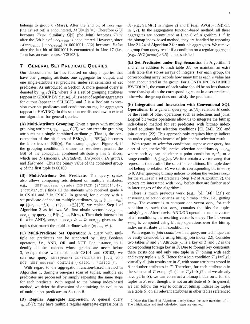
Fig. 5. Overall comparison of the methods, O=⊆, C=10. (Execution time is in logarithmic scale.)

on three different datasets– (1) Our own synthetic data (Sec-tion 9.2 (A)), for studying the effect of various parametersin the performance of these methods, including the numberof tuples, the number of groups, the number of values in aset predicate, the number of qualified groups, and so on; (2)TPC-H benchmark database (Section 9.2 (B)), for studyingthe performance of these methods on general queries with joinconditions and on benchmark data capturing the characteristicsof decision support applications; (3) WorldCup98 dataset (Sec-tion 9.2 (C)), for evaluating the performance of the methodson real and big data.

The aggregate function-based method, denoted asAgg,is implemented in C++. The bitmap index-based method,denoted asBitmap, is also implemented in C++ and leveragesFastBit 4 for bit-sliced index implementation. The compres-sion scheme of FastBit, Word-Aligned Hybrid (WAH) code,makes the compressed bitmap indices efficient even for high-cardinality attributes [33].

The method of using regular SQL to express set-levelcomparisons is denoted asRewrt. We used PostgreSQL 8.3.7to store data and execute regular SQL queries. In the sup-plemental materials to this paper, we describe how to rewritequeries with set predicate into regular SQL. It is not a com-plete enumeration of all possible query rewritings becauseinpractice there will be infinite possible rewritings. We madeourbest effort to express each query by an appropriate regular SQLquery and obtain an efficient query plan for the query. This wasdone by manually investigating alternative queries and plansand turning on/off various physical query operators. Belowwe report the numbers obtained by these hand-picked plans.Nevertheless, the queries we often used for CONTAINED BYare in the form of the rewriting in Figure 2. For a CONTAINpredicate withm values, we often used a query that intersectsthe results ofm selection queries on the individual values. Thisrewriting approach can be found in the supplemental materialsto this paper.

Note thatRewrt uses a full-fledged database engine Post-greSQL, while bothAgg and Bitmap are implemented ex-ternally. AlthoughRewrt would incur extra overhead fromquery optimizer, tuple formatting, etc., we believe this com-parison is still insightful. Our results show thatRewrt isoften one or more orders of magnitude less efficient. It isunlikely that all the slowness comes from extra overheads.Moreover the query plans resulting from regular SQL queriesdiscussed in Section 4 ultimately perform one-pass groupingand aggregation upon the results of (multiple) other upstreamoperations. Therefore the performance ofAgg, which is alsoimplemented externally, serves as a yardstick in comparison

4. https://sdm.lbl.gov/fastbit.

parameter meaning values

O set operators ⊇, ⊆, =C number of values in set

predicate1, 2, . . . , 10, 20,. . . , 100

T number of tuples 10K,100K, 1MG number of groups 10,100,. . . ,TS number of qualified groups 1,10,. . . ,G

TABLE 1Configuration parameters of synthetic data experiments.

with the performance ofBitmap. Hence the results verifythat using regular SQL queries obscures the semantics of set-level comparisons and leads to costly plans. The results couldencourage vendors to incorporate the proposed approaches intoa database engine.

9.2 Results

The experiments were performed on a Dell PowerEdge 2900III server with Linux kernel 2.6.27, dual quad-core Xeon2.0GHz processors, 2x4MB cache, 8GB RAM, and three146GB 10K-RPM SCSI hard drivers in RAID5. The reportedresults are the averages of 10 runs. All performance data wereobtained with cold buffer.

(A) Comparison over synthetic data:

Queries: We evaluated the three methods under various com-binations of parameters, which are summarized in Table 1.Ocan be one of the 3 set operators (⊇,⊆,=). C is the number ofvalues in a predicate, varying from 1 to 10, then 10 to 100. Thevalues always start from 1 and increase by 1, i.e., the valuesare{1, . . . , C}. Altogether we have 3×19 (O,C) pairs. Eachpair corresponds to a unique query with a single set predicate.For instance,(⊇, 2) corresponds toQ=γg,SUM(a)v⊇{1, 2}(R).Note that we assume SUM is the aggregate function since itsevaluation is not our focus and Algorithm 1 and 2 process allaggregate functions in the same way.

Data: For each of the 3×19 single-predicate queries, wegenerated 61 data tables, each corresponding to a differentcombination of (T,G, S) values in Table 1. Given query(O,C) and data statistics(T,G, S), we correspondingly gen-erated a table that satisfies the statistics for the query. The tablehas schemaR(a, v, g), for queryγg,SUM(a)v O {1, ..., C}(R).

Each column is a 4-byte integer. The values of columnaare randomly generated. The values in columng are generatedby following a uniform distribution, to make sure there areGgroups, i.e., there are aboutT /G tuples in each group. Werandomly chooseS out of the G groups to be qualifyinggroups. For the tuples in each qualifying group, we generatetheir values on columnv in a way such that the groupsatisfies the set predicate. Thev values for theG-S disqualified

11

groups are similarly generated, by making sure the groupscannot satisfy the set predicate. For example, if the queryis γg,SUM(a)v⊇{1, 2}(R), for a qualified group, we randomlyselect 2 tuples and set theirv values to 1 and 2, respectively.The v values for remaining tuples in the group are generatedrandomly. Given a group to be disqualified, we randomlydecide if 1, 2, or both should be missing from the group,and generate the values randomly from a pool of numbersexcluding the missing values.

Results: We measured wall-clock execution time ofRewrt,Agg, and Bitmap over the aforementioned 61 data tables foreach of the 3×19 queries. The comparison of these methodsunder different queries are fairly similar. Hence we only showthe results for one query for data table 0-60 in Figure 5:γg,SUM(a)v ⊆ {1, . . . , 10}(R). For instance, data table 54 inFigure 5 represents results of the three methods withT=1 mil-lion, G=100K, S=100K, under queryO=⊆, C=10. Note thatthe purpose of the figure is not to compare the performanceon different data tables. (Such detailed comparison is providedin Figure?? in the supplemental materials to this paper.) It israther to show the performance gap between several algorithmsthat is consistently observed in all data tables under variousqueries.

Figure 5 shows thatBitmap is often several times moreefficient than Agg and is usually one order of magnitudefaster thanRewrt. The low efficiency ofRewrt is due to theawkwardness of expressing set-level comparisons by regularSQL and the difficulty in optimizing such queries. The per-formance advantage ofAgg over Rewrtshows that the simplequery algorithm could improve efficiency significantly. Theshown advantage ofBitmap over Agg is due to fast bit-wiseoperations and skipping enabled by bitmap index, comparedto the verbatim comparisons used byAgg.

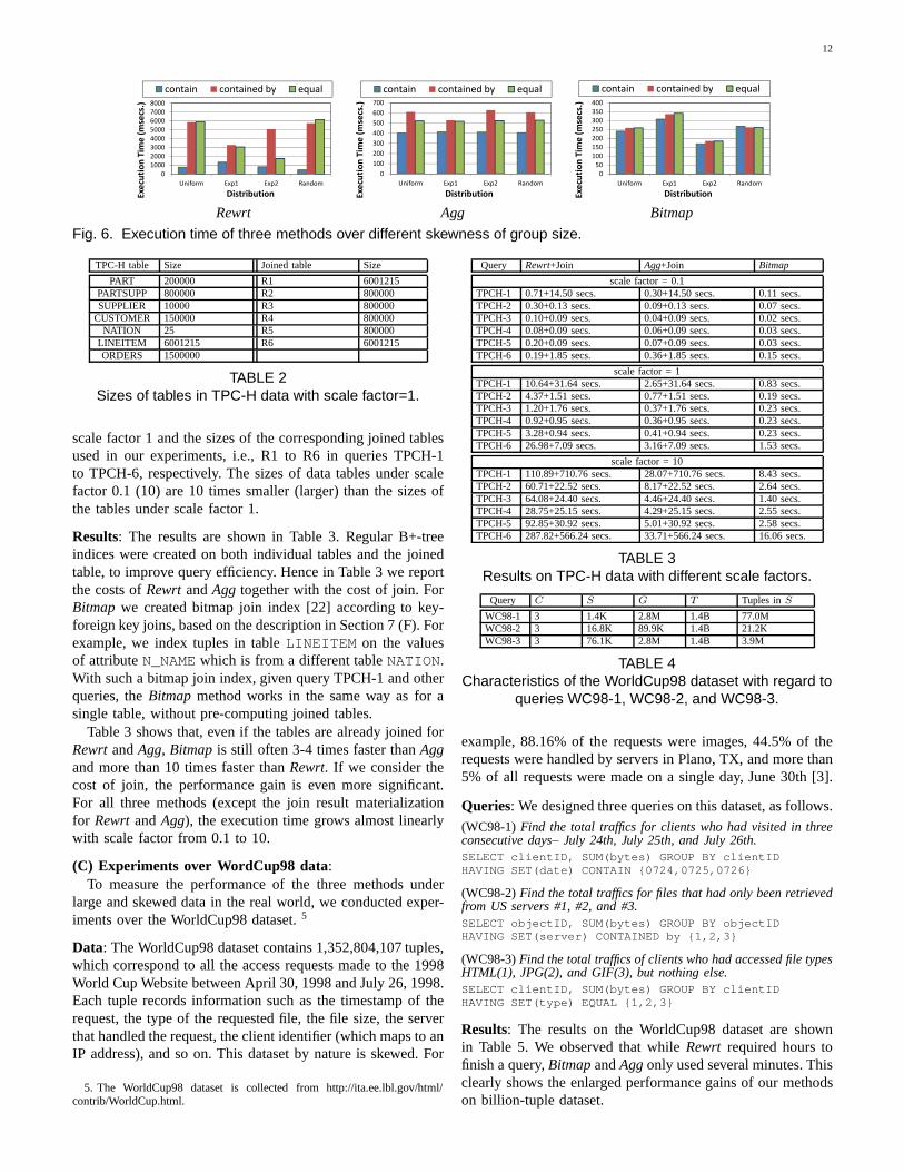
Impact of the Skewness of Group Sizes: Since the groupingattribute values in the synthetic data were generated by uni-form distributions, the groups in a table have about the samesize (i.e., number of tuples). To further study the impact ofskewness of group sizes on the several methods’ performance,we generated more data tables. Given a combination of fixedvalues on the four configuration parametersC, T , G, andS,we generated 4 different data tables, by varying group sizedistribution– (1)Uniform, where the grouping attribute valuesfollow a uniform distribution, thus the sizes of different groupstend to be equal. Note that this is the same as the data usedin Figure 5. (2)Random, where the group size is a randomvariable in a given range. (3)Exp1andExp2, where the sizesof groups follow an exponential distribution(1/2)n, in whichn is the variable for group size. A small constant is used whena group size generated by the distribution is smaller than 1.Exp1andExp2are two opposite cases, in which the sizes ofqualified groups are all large and small, respectively.

Figure 6 shows the results of this experiment underC=4,T=1M , G=1K, andS=10, for which theUniform data tablecorresponds to data table 40 in Figure 5. We can make thefollowing observations. (1) The skewness of group size hadlarge impact on the performance ofRwrt, especially for CON-TAINED BY and EQUAL operations. Consider CONTAINED

BY. The execution time ofRwrt decreased when qualifiedgroups are large (Exp1). Based on the way the skewed datawas generated, the larger the qualified groups are, the moretuples matching the values in set predicates. Therefore theoutput cardinality of the Filter operation in Figure 2 wassubstantially reduced underExp1. In contrast, when qualifiedgroups are small (Exp2), the Filter operation produced largeoutput, which increased the cost of the query method in thiscase. For EQUAL operation, the performance can also beanalyzed similarly based on the query plan generated, whichis omitted here. (2) The skewness of group size did not havemuch effect on the performance ofAgg. This is becauseAggalways sequentially scans the whole table, regardless of the setoperation and the skewness of group size. (3) The skewnessof group size had some impact on the performance ofBitmap,although not as much as onRewrt. Consider CONTAINoperation. Step 3 and Step 4 (and thus the wholeBitmapmethod) in Algorithm 2 are more expensive when there aremore tuples matching the values in set predicates (Exp1). Itbecomes the opposite case when qualified groups are small(Exp2). For all the methods, the performance onRandomis notmuch different from that onUniform, because the numbers oftuples matching the values in set predicates only differ slightlyin the two data tables.

(B) Experiments over TPC-H data:Two of the advantages ofBitmap mentioned in Section 6

could not be demonstrated by the above experiment. First,it only needs to process necessary columns, whileAgg andRewrt have to scan the full table before irrelevant columnscan be projected out. The tables used in the experiments forFigure 5 have schemaR(a, v, g) which does not include othercolumns. We can expect the costs ofRewrtandAggto increaseby table width, whileBitmap will stay unaffected. Second,Bitmapenables seamless integration with selections and joins,while the above experiment is on a single table.

Queries: We thus designed six queries (TPCH-1 below,TPCH-2 to TPCH-6 in the supplemental materials to this pa-per) on the TPC-H benchmark database [31] and compared theperformance of the three methods. In these queries, groupingand set predicates are defined over the join result of multipletables. Note that the joins are key-foreign key joins. ForRewrtandAgg, we first joined the tables to generate a single joinedtable, and then executed the algorithms over that joined table.

(TPCH-1)Get the total sales of each brand that has business in bothUSA and Canada.CREATE VIEW R1 ASSELECT P_BRAND, L_QUANTITY, N_NAMEFROM LINEITEM, ORDERS, CUSTOMER, PART, NATIONWHERE L_ORDERKEY=O_ORDERKEY

AND O_CUSTKEY=C_CUSTKEYAND C_NATIONKEY=N_NATIONKEYAND L_PARTKEY=P_PARTKEY;

SELECT P_BRAND, SUM(L_QUANTITY) FROM R1GROUP BY P_BRANDHAVING SET(N_NAME) CONTAIN {’United States’,’Canada’}

Data: The data tables were generated by the TPC-H datagenerator, with scale factors 0.1, 1, and 10, respectively.Table 2 shows the sizes of the original TPC-H tables under

12

3000

4000

5000

6000

7000

8000

Exe

cuti

on

Tim

e (

mse

cs.)

contain contained by equal

0

1000

2000

3000

Uniform Exp1 Exp2 Random

Exe

cuti

on

Tim

e (

mse

cs.)

Distribution

200

300

400

500

600

700

Exe

cuti

on

Tim

e (

mse

cs.)

contain contained by equal

0

100

200

Uniform Exp1 Exp2 Random

Exe

cuti

on

Tim

e (

mse

cs.)

Distribution

150

200

250

300

350

400

Exe

cuti

on

Tim

e (

mse

cs.)

contain contained by equal

0

50

100

150

Uniform Exp1 Exp2 Random

Exe

cuti

on

Tim

e (

mse

cs.)

Distribution

Rewrt Agg Bitmap

Fig. 6. Execution time of three methods over different skewness of group size.

TPC-H table Size Joined table Size

PART 200000 R1 6001215PARTSUPP 800000 R2 800000SUPPLIER 10000 R3 800000

CUSTOMER 150000 R4 800000NATION 25 R5 800000

LINEITEM 6001215 R6 6001215ORDERS 1500000

TABLE 2Sizes of tables in TPC-H data with scale factor=1.

scale factor 1 and the sizes of the corresponding joined tablesused in our experiments, i.e., R1 to R6 in queries TPCH-1to TPCH-6, respectively. The sizes of data tables under scalefactor 0.1 (10) are 10 times smaller (larger) than the sizes ofthe tables under scale factor 1.

Results: The results are shown in Table 3. Regular B+-treeindices were created on both individual tables and the joinedtable, to improve query efficiency. Hence in Table 3 we reportthe costs ofRewrtandAgg together with the cost of join. ForBitmap we created bitmap join index [22] according to key-foreign key joins, based on the description in Section 7 (F).Forexample, we index tuples in tableLINEITEM on the valuesof attributeN_NAME which is from a different tableNATION.With such a bitmap join index, given query TPCH-1 and otherqueries, theBitmap method works in the same way as for asingle table, without pre-computing joined tables.

Table 3 shows that, even if the tables are already joined forRewrtandAgg, Bitmap is still often 3-4 times faster thanAggand more than 10 times faster thanRewrt. If we consider thecost of join, the performance gain is even more significant.For all three methods (except the join result materializationfor RewrtandAgg), the execution time grows almost linearlywith scale factor from 0.1 to 10.

(C) Experiments over WordCup98 data:To measure the performance of the three methods under

large and skewed data in the real world, we conducted exper-iments over the WorldCup98 dataset.5

Data: The WorldCup98 dataset contains 1,352,804,107 tuples,which correspond to all the access requests made to the 1998World Cup Website between April 30, 1998 and July 26, 1998.Each tuple records information such as the timestamp of therequest, the type of the requested file, the file size, the serverthat handled the request, the client identifier (which maps to anIP address), and so on. This dataset by nature is skewed. For

5. The WorldCup98 dataset is collected from http://ita.ee.lbl.gov/html/contrib/WorldCup.html.

Query Rewrt+Join Agg+Join Bitmap

scale factor = 0.1TPCH-1 0.71+14.50 secs. 0.30+14.50 secs. 0.11 secs.TPCH-2 0.30+0.13 secs. 0.09+0.13 secs. 0.07 secs.TPCH-3 0.10+0.09 secs. 0.04+0.09 secs. 0.02 secs.TPCH-4 0.08+0.09 secs. 0.06+0.09 secs. 0.03 secs.TPCH-5 0.20+0.09 secs. 0.07+0.09 secs. 0.03 secs.TPCH-6 0.19+1.85 secs. 0.36+1.85 secs. 0.15 secs.

scale factor = 1TPCH-1 10.64+31.64 secs. 2.65+31.64 secs. 0.83 secs.TPCH-2 4.37+1.51 secs. 0.77+1.51 secs. 0.19 secs.TPCH-3 1.20+1.76 secs. 0.37+1.76 secs. 0.23 secs.TPCH-4 0.92+0.95 secs. 0.36+0.95 secs. 0.23 secs.TPCH-5 3.28+0.94 secs. 0.41+0.94 secs. 0.23 secs.TPCH-6 26.98+7.09 secs. 3.16+7.09 secs. 1.53 secs.

scale factor = 10TPCH-1 110.89+710.76 secs. 28.07+710.76 secs. 8.43 secs.TPCH-2 60.71+22.52 secs. 8.17+22.52 secs. 2.64 secs.TPCH-3 64.08+24.40 secs. 4.46+24.40 secs. 1.40 secs.TPCH-4 28.75+25.15 secs. 4.29+25.15 secs. 2.55 secs.TPCH-5 92.85+30.92 secs. 5.01+30.92 secs. 2.58 secs.TPCH-6 287.82+566.24 secs. 33.71+566.24 secs. 16.06 secs.

TABLE 3Results on TPC-H data with different scale factors.

Query C S G T Tuples inS

WC98-1 3 1.4K 2.8M 1.4B 77.0MWC98-2 3 16.8K 89.9K 1.4B 21.2KWC98-3 3 76.1K 2.8M 1.4B 3.9M

TABLE 4Characteristics of the WorldCup98 dataset with regard to

queries WC98-1, WC98-2, and WC98-3.

example, 88.16% of the requests were images, 44.5% of therequests were handled by servers in Plano, TX, and more than5% of all requests were made on a single day, June 30th [3].

Queries: We designed three queries on this dataset, as follows.(WC98-1)Find the total traffics for clients who had visited in threeconsecutive days– July 24th, July 25th, and July 26th.SELECT clientID, SUM(bytes) GROUP BY clientIDHAVING SET(date) CONTAIN {0724,0725,0726}

(WC98-2)Find the total traffics for files that had only been retrievedfrom US servers #1, #2, and #3.SELECT objectID, SUM(bytes) GROUP BY objectIDHAVING SET(server) CONTAINED by {1,2,3}

(WC98-3)Find the total traffics of clients who had accessed file typesHTML(1), JPG(2), and GIF(3), but nothing else.SELECT clientID, SUM(bytes) GROUP BY clientIDHAVING SET(type) EQUAL {1,2,3}

Results: The results on the WorldCup98 dataset are shownin Table 5. We observed that whileRewrt required hours tofinish a query,BitmapandAggonly used several minutes. Thisclearly shows the enlarged performance gains of our methodson billion-tuple dataset.

13

Query Rewrt Agg Bitmap

WC98-1 16061 secs. 569 secs. 427 secs.WC98-2 20692 secs. 698 secs. 380 secs.WC98-3 15571 secs. 689 secs. 468 secs.

TABLE 5Results on the WorldCup98 dataset.

200

250

300

350

400

450

500

Exe

cuti

on

Tim

e (

mse

cs.)

WC98-1 WC98-2 WC98-3

0

50

100

150

200

25% 50% 75% 100%Exe

cuti

on

Tim

e (

mse

cs.)

T

200

300

400

500

600

Exe

cuti

on

Tim

e (

mse

cs.)

WC98-1 WC98-2 WC98-3

0

100

200

25% 50% 75% 100%Exe

cuti

on

Tim

e (

mse

cs.)

C

Fig. 7. Execution time of Bitmap on the WorldCup98dataset under different data sizes and query complexities.

We further investigated howBitmapperforms under differ-ent table sizes and query complexities. We varied number oftuples (T ) by using 20%, 50%, 75%, and 100% of the originaldataset. We varied number of values in set predicate (C) byusing 20%, 50%, 75%, and 100% of the distinct attributevalues in the original dataset as the values in set predicate. Theresults are shown in Figure 7. The execution time ofBitmapgrew linearly by the data size and grew very slowly by thequery complexity.

Below we explain the results in Table 5. For better under-standing of the results, we list in Table 4 the characteristics ofthe dataset with regard to the three queries. In addition to thefour variables–number of values in set predicate (C), numberof qualified groups (S), number of groups (G), and number oftuples (T )–Table 4 also shows the number of tuples in qualifiedgroups (Tuples inS). Note that the focus of the analysis is tounderstand the individual results. It is not to say which query ismore efficient than others. The three queries are different in setoperations (i.e. CONTAIN, CONTAINED BY, and EQUAL),set predicate attributes, and grouping attributes. Hence it is lessmeaningful to compare the three queries against each other,as the performance of a query can be highly dependent on theparametersC, S, G, Tand skewness of data.

ForRewrt, the performance difference between WC98-1 andWC98-3 was small. WC98-2 was considerably less efficient.From Figure 2, we can see that the query plan needs to performa set difference operation between the original table and theset of tuples that do not match any set predicate values. Inquery WC98-2, many tuples did not match the set predicatevalues. That made the set difference operation expensive.For Agg, query WC98-1 took less time than the other twoqueries. This can be explained by our observation thatAgg issensitive to data sizeT and less sensitive to other parametersand under the same data size CONTAIN operation is moreefficient than CONTAINED BY and EQUAL with regard toAgg (cf. Figure 6 and supplemental materials). ForBitmap,query WC98-2 had the best performance since it had muchfewer groups and tuples in qualified groups, in comparisonwith WC98-1 and WC98-3 (cf. Table 4). This is also consistentwith the observation in Section 9.2 (A).

estimated selectivity real selectivityp11 99.88% 95.71%

MPQ1 p12 62.88% 80.32%p13 25.75% 15.79%p21 99.99% 95.56%

MPQ2 p22 69.54% 83.81%p23 13.16% 9.61%p31 99.95% 90.09%

MPQ3 p32 73.51% 35.61%p33 13.87% 20.13%

TABLE 6Comparison of estimated and real selectivity.

MPQ1 (i=1) MPQ2 (i=2) MPQ3 (i=3)plan1: pi1pi2pi3 0.69 0.79 0.68plan2: pi1pi3pi2 0.69 0.79 0.68plan3: pi2pi1pi3 0.69 0.79 0.68plan4: pi2pi3pi1 0.31 0.33 0.16plan5: pi3pi1pi2 0.69 0.79 0.68plan6: pi3pi2pi1 0.32 0.33 0.16

TABLE 7Execution time of different plans (in seconds).

(D) Selectivity estimation and predicate ordering:We also conducted experiments to verify the accuracy andeffectiveness of the selectivity estimation method in Section 8.Here we use the results of three queries (MPQ1, MPQ2,MPQ3), each on a different synthetic data table, to demon-strate. The values of grouping attributeg and set predicate at-tributev are independently generated, each following a normaldistribution. Each MPQi has three conjunctive set predicates,pi1, pi2, andpi3. The predicates are manually chosen so thatthey have different selectivities, shown in the real selectivitycolumn of Table 6. Predicatepi3 is most selective, with 10%to 20% qualified groups;pi1 is least selective, with around90% qualified groups;pi2 has a selectivity in between.

To estimate set predicate selectivity, we employed twohistograms overg and v, respectively. The data tables haveabout 40−60 distinct values inv and 10000 distinct valuesin g. We built 10 and 100 equi-width buckets, onv and g,respectively. Table 6 shows that the estimated selectivities aresufficiently accurate to capture the order of different predicatesby selectivity.

Table 7 shows that our method is effective in choosingefficient query plans. As discussed in Section 8, based onestimated selectivity, our optimization method chooses a planthat evaluates conjunctive predicates in the ascending order ofselectivity. The execution terminates early when the evaluatedpredicates result in empty qualified groups. Given each queryMPQi, there are 6 possible orders in evaluating three predi-cates, shown as plan1−plan6 in Table 7. Since the order ofestimated selectivity ispi3 < pi2 < pi1, our method choosesplan6 over other plans, based on the speculation that it has abetter chance to stop the evaluation earlier. Plan6 evaluatespi3first, followed bypi2, and finallypi1 if necessary.

In all three queries, the chosen plan6 terminated afterpi3 and pi2, because no group satisfies both predicates. Bycontrast, other plans (except plan4) evaluated all predicates.Therefore their execution time is 3 to 4 times of that of plan6.Note that plan6 saves the cost by about 60%, by just avoidingpi1 out of 3 predicates. This is due to different evaluation costsof predicates. The least selective predicate,pi1, naturally is

14

also the most expensive one. This indicates that, selectivityand cardinality will be the basis of cost-model in a cost-basedquery optimizer for set predicates, consistent with the commonpractice in DBMSs. We also note that plan4 is equally efficientas plan6 for these queries, because they both terminate afterpi2 andpi3 and no plan can stop after only one predicate.

10 CONCLUSION

We propose to extend SQL by set predicates to support set-level comparisons. Such predicates, combined with grouping,allow selection of dynamically formed groups by comparisonbetween a group and a set of values. We presented twoevaluation methods to process set predicates. Comprehensiveexperiments on synthetic and TPC-H data show the effective-ness of both the aggregate function-based approach and thebitmap index-based approach. For optimizing multi-predicatequeries, we designed a histogram-based probabilistic methodto estimate the selectivity of set predicates. The estimationgoverns the evaluation order of multiple predicates, producingefficient query plans.

ACKNOWLEDGMENT

This material is based upon work partially supported byNSF Grant IIS-1018865, CCF-1117369, and 2011, 2012 HPLabs Innovation Research Award. Any opinions, findings, andconclusions or recommendations expressed in this publicationare those of the author(s) and do not necessarily reflect theviews of the funding agencies. The authors would also like tothank the anonymous reviewers for their valuable commentsand suggestions to improve the quality of the paper.

REFERENCES

[1] Jaql: Query language for javascript object notation (json).http://code.google.com/p/jaql/.

[2] G. Antoshenkov. Byte-aligned bitmap compression. InProceedings ofthe Conference on Data Compression, 1995.

[3] M. Arlitt and T. Jin. A workload characterization study of the 1998world cup web site.IEEE Network, 14(3):30 –37, 2000.

[4] D. Chamberlin, M. Astrahan, K. Eswaran, P. Griffiths, R. Lorie, J. Mehl,P. Reisner, and B. Wade. Sequel 2: A unified approach to data definition,manipulation, and control.IBM Journal of R & D, 20(6):560 –575, 1976.

[5] C. Y. Chan and Y. E. Ioannidis. An efficient bitmap encoding schemefor selection queries. InSIGMOD, 1999.

[6] A. K. Chandra and P. M. Merlin. Optimal implementation ofconjunctivequeries in relational data bases. InSTOC, 1977.

[7] D. Chatziantoniou. Using grouping variables to expresscomplexdecision support queries.Data Knowl. Eng., 61(1):114–136, 2007.

[8] D. Chatziantoniou and K. A. Ross. Querying multiple features of groupsin relational databases. InVLDB, pages 295–306, 1996.

[9] D. Chatziantoniou and K. A. Ross. Groupwise processing of relationalqueries. InVLDB, pages 476–485, 1997.

[10] D. Chatziantoniou and E. Tzortzakakis. Asset queries:a declarativealternative to mapreduce.SIGMOD Rec., 38(2):35–41, Oct. 2009.

[11] R. Elmasri and S. Navathe. Fundamentals of Database Systems.Addison-Wesley, 2011.

[12] G. Graefe and R. L. Cole. Fast algorithms for universal quantificationin large databases.ACM TODS, 20(2), 1995.

[13] J. M. Hellerstein and M. Stonebraker. Predicate migration: optimizingqueries with expensive predicates. InSIGMOD, pages 267–276, 1993.

[14] S. Helmer and G. Moerkotte. Evaluation of main memory join algo-rithms for joins with set comparison join predicates. InVLDB, 1996.

[15] Y. Ioannidis. The history of histograms (abridged). InVLDB, 2003.[16] T. Johnson. Performance measurements of compressed bitmap indices.

In VLDB, pages 278–289, 1999.

[17] P.-A. Larso. Grouping and duplicate elimination: Benefits of earlyaggregation. Technical report, 1997.

[18] N. Mamoulis. Efficient processing of joins on set-valued attributes. InSIGMOD, pages 157–168, 2003.

[19] S. Melnik and H. Garcia-Molina. Adaptive algorithms for set contain-ment joins.ACM Trans. Database Syst., 28(1):56–99, 2003.

[20] S. Melnik, A. Gubarev, J. J. Long, G. Romer, S. Shivakumar, M. Tolton,and T. Vassilakis. Dremel: interactive analysis of web-scale datasets.Commun. ACM, 54:114–123, June 2011.

[21] C. Olston, B. Reed, U. Srivastava, R. Kumar, and A. Tomkins. Piglatin: a not-so-foreign language for data processing. InSIGMOD, pages1099–1110, 2008.

[22] P. E. O’Neil and G. Graefe. Multi-table joins through bitmapped joinindices. SIGMOD Record, 24(3):8–11, 1995.

[23] P. E. O’Neil and D. Quass. Improved query performance with variantindexes. InSIGMOD, pages 38–49, 1997.

[24] G. Ozsoyoglu, Z. M.Ozsoyoglu, and V. Matos. Extending relationalalgebra and relational calculus with set-valued attributes and aggregatefunctions. ACM TODS, 12(4), 1987.

[25] V. Poosala, P. J. Haas, Y. E. Ioannidis, and E. J. Shekita. Improvedhistograms for selectivity estimation of range predicates. SIGMOD Rec.,25(2):294–305, 1996.

[26] V. Poosala and Y. E. Ioannidis. Selectivity estimationwithout theattribute value independence assumption. InVLDB, 1997.

[27] K. Ramasamy, J. Patel, R. Kaushik, and J. Naughton. Set containmentjoins: The good, the bad and the ugly. InVLDB, 2000.

[28] D. Rinfret, P. O’Neil, and E. O’Neil. Bit-sliced index arithmetic. InSIGMOD, pages 47–57, 2001.

[29] M. Roth, H. Korth, and A. Silberschatz. Extended algebra and calculusfor nested relational databases.TODS, 1988.

[30] M. Stonebraker, D. Abadi, A. Batkin, X. Chen, M. Cherniack, M. Fer-reira, E. Lau, A. Lin, S. Madden, E. O’Neil, P. O’Neil, A. Rasin, N. Tran,and S. Zdonik. C-store: A column oriented dbms. InVLDB, 2005.

[31] Transaction Processing Performance Council. TPC benchmark H (deci-sion support) standard specification. 2009.

[32] K. Wu, E. Otoo, and A. Shoshani. On the performance of bitmap indicesfor high cardinality attributes. InVLDB, 2004.

[33] K. Wu, E. J. Otoo, and A. Shoshani. Optimizing bitmap indices withefficient compression.ACM TODS, 31(1), 2006.

[34] M.-C. Wu and A. P. Buchmann. Encoded bitmap indexing fordatawarehouses. InICDE, pages 220–230, 1998.

Chengkai Li is an Assistant Professor in the Department of ComputerScience and Engineering at the University of Texas at Arlington. Hisresearch interests are in the areas of databases, Web data manage-ment, data mining, and information retrieval. In particular, he workson computational journalism, database exploration, database testing,entity search and query, and ranking and skyline queries. He receivedhis Ph.D. degree in Computer Science from the University of Illinoisat Urbana-Champaign in 2007, and an M.E. and a B.S. degree inComputer Science from Nanjing University, China, in 2000 and 1997,respectively.

Bin He is a Research Staff Member and Master Inventor at IBMAlmaden Research. He got his Ph.D. in the Department of ComputerScience at the University of Illinois at Urbana-Champaign in 2006. Healso received the M.S. degree in Computer Science from the Universityof Illinois at Urbana-Champaign in 2002, and M.S. and B.S. degreesin Mathematics from Peking University, China in 2000 and 1998 respec-tively. He has strong expertise in business intelligence, cloud computing,databases, data warehousing, data mining, and data integration.

Ning Yan received his B.E. degree in software engineering and M.S.degree in computer science from Southeast University in China. He iscurrently a Ph.D. candidate in the Department of Computer Scienceand Engineering at the University of Texas at Arlington. His researchinterests include faceted search, entity retrieval, and database system.

Muhammad Assad Safiullah received his M.S. degree in ComputerScience from the University of Texas at Arlington in 2008 and his B.S.degree in Computer Science from the National University of Computerand Emerging Sciences, Islamabad, Pakistan in 2005. His M.S. thesisfocused on efficient processing of set-predicate queries using bitmapindexes. He is currently a software engineer at Microsoft Corporation.

1

Supplemental Materials to “Set Predicates in SQL:Enabling Set-Level Comparisons for Dynamically FormedGroups”

A DETAILS OF THE QUERY REWRITING AP-PROACH

We can formally prove by relational algebra that a query withset predicates can be translated into standard SQL queries.There could be multiple ways in rewriting a query. We willnot enumerate all of them.

First, it is easy to showγG,AC(R) = γG,A(R ⊲⊳ γGC(R)).

γGC(R) selects the qualified groups. Joining the qualifiedgroups withR on grouping attributes and then computingaggregates will generate the correct query results.

Now we consider the rewriting ofγGC(R). Given twopredicates, i.e.,C = C1 AND|OR C2, we rewrite for eachset predicate separately and then put them together, by usingINTERSECT for AND and UNION for OR.γGC1 AND C2 (R) = γGC1 (R) ∩ γGC2 (R)γGC1 OR C2 (R) = γGC1 (R) ∪ γGC2 (R)Given a predicate with a preceding NOT, i.e.,C = NOT C′,

we rewrite by using set difference operation.γG NOT C′ (R) = πG(R) − γG C′ (R)If C contains multiple predicatesC1 ... Cm connected by

Boolean operators (AND, OR, NOT), we rewrite by keepapplying the above algebraic rules.

Now we focus on how to rewrite a single set predicate. ACONTAIN predicateC ⊇ {c1, ..., cn} can be rewritten by:γGC ⊇ {c1, ..., cn}(R) = πGσC=c1(R) ∩ ... ∩ πGσC=cn (R)A CONTAINED BY predicateC ⊆ {c1, ..., cn} can be

rewritten by:γGC ⊆ {c1, ..., cn}(R) = πG(R) - πGσC6=c1∧...∧C6=cn(R)An EQUAL predicateC = {c1, ..., cn}, which is a combi-

nation of CONTAIN and CONTAINED BY, is rewritten by:γGC = {c1, ..., cn}(R) =(πGσC=c1 (R) ∩ ... ∩ πGσC=cn (R)) - πGσC6=c1∧...∧C6=cn(R)Below are some examples to show how to apply the above

algebraic rules in query rewriting.

Rewriting CONTAIN : Consider the query Q1 in Section 3,which has a CONTAIN predicate. It can be rewritten usingINTERSECT, as shown in the following Q1’. In general, aCONTAIN predicate withm constant values can be rewrittenusingm-1 INTERSECT operations. Note that INTERSECT,UNION, and EXCEPT in SQL operate by set semanticsinstead of bag semantics, unless they are followed by ALL.

Q1’: SELECT student FROM SC WHERE course = ’CS101’INTERSECTSELECT student FROM SC WHERE course = ’CS102’

If the SELECT clause in the query contains aggregatevalues, the rewritten query needs to be joined with the originaltable on the grouping attributes. For instance, suppose theSELECT clause in Q1 isSELECT student,COUNT(*),i.e., we want to identify the qualifying students and the numberof courses that they have taken, the rewritten query will be:

SELECT student, COUNT(*)

FROM SC,(SELECT student FROM SC WHERE course = ’CS101’INTERSECTSELECT student FROM SC WHERE course = ’CS102’

) as TMPWHERE SC.student = TMP.studentGROUP BY student

Alternatively a subquery instead of join can be used toobtain the aggregate values:

SELECT student, COUNT(*)FROM SCWHERE student IN

(SELECT student FROM SC WHERE course = ’CS101’INTERSECTSELECT student FROM SC WHERE course = ’CS102’

) as TMPGROUP BY student

Rewriting CONTAINED BY : The CONTAINED BY pred-icate can be rewritten by using EXCEPT. For instance, therewritten query for Q3 in Section 3 is:

Q3’: SELECT student FROM SCEXCEPTSELECT student FROM SCWHERE grade <> 4 AND grade <> 3

Rewriting EQUAL : The rewriting of EQUAL predicatesnaturally combines that of CONTAIN and CONTAINED BY,since two setsS1 = S2 if and only if S1 ⊆ S2 andS1 ⊇ S2.For instance, Q4 in Section 3 can be rewritten as:

Q4’:(SELECT student FROM SC WHERE course = ’CS101’INTERSECTSELECT student FROM SC WHERE course = ’CS102’)

EXCEPT(SELECT student FROM SCWHERE course <> ’CS101’ AND course <> ’CS102’)

Rewriting General Queries: To rewrite more complex querieswith multiple predicates, we use the rewriting of individualpredicates as the building blocks and connect them togetherby their logical relationships. For instance, given the followingquery:

SELECT student,AVG(grade) FROM SC GROUP BY studentHAVING MAX(grade) = 4OR SET(course) CONTAIN {’CS101’, ’CS102’}OR SET(course) CONTAIN {’CS101’, ’CS103’}

The rewritten query is:

SELECT student, AVG(grade)FROM SC,

((SELECT student FROM SC GROUP BY studentHAVING MAX(grade) = 4)

UNION (SELECT student FROM SC WHERE course=’CS101’INTERSECTSELECT student FROM SC WHERE course=’CS102’)

UNION (SELECT student FROM SC WHERE course=’CS101’INTERSECTSELECT student FROM SC WHERE course=’CS103’)

) as TMPWHERE SC.student = TMP.studentGROUP BY student

Moreover, as mentioned in Section 3, the grouping and setpredicates can be defined over a relationR that is the resultof a subquery. Even though our examples only use a singletable, the general applicability is straightforward.

2

B GENERAL SET PREDICATE QUERIES (SEC-TION 7 CONT’D)(G) Range-Based Set Predicate: Set predicates on data typessuch as numeric attributes and dates can use range-basedvalues (e.g., Example 3 in Section 1), in two different ways.

(1) The operand is a set and a value in this set canbe a range. For example, predicateSET(size) CONTAIN

{[1,10],[25,30)} requires a group to have at least twosize

values such that the first one is within range [1,10] and the sec-ond one is within range [25,30). A group such as{3,4,15,27}would qualify because 3 (4 too) satisfies the first range and 27satisfies the second range. Similarly{3,15} does not satisfySET(size) CONTAINED BY {[1,10], [25,30)} because15 is not in either [1,10] or [25,30).

With regard to the bitmap index-based method, we modifyLine 1 and 2 of Algorithm 2. TheQueryBI function returnsa bit vector for each range, which is naturally supported byboth bit-sliced index and regular bitmap indices [28], [32]. Forextending the aggregate function-based method, we replacev==vj by v ∈ rangej in Line 8 of Algorithm 1.

(2) The whole operand itself is a range. For example,predicateSET(size) CONTAINED BY [1,10] requires thevalues ofsize in a qualified group to be subsumed by{1, 2,. . . , 10}. Another example isSET(size) CONTAIN [1,10]

which requires a group to subsume{1, 2, . . . , 10}. Note thatsuch a CONTAIN predicate is not meaningful on attribute offloating point numbers.

With regard to the bitmap index-based method, we replaceLine 1 and 2 of Algorithm 2 by aQueryBI function toobtain a bit vector for the range. For extending the aggregatefunction-based method, we replacev == vj by v ∈ range inLine 8 of Algorithm 1.

(H) Set-Level Comparisons with Subquery Results,between Multiple Groups, and with Partial Satisfaction:The syntax in Section 3 can be extended to allowcomparison with not only literal values, but also theresult of a subquery. An example query isSELECT student

FROM SC GROUP BY student HAVING SET (course)

CONTAINED BY (SELECT course_id FROM Courses

WHERE dept=’CS’). (Finding those students that have onlytaken CS courses.) The impact of such extension on theproposed evaluation approaches is minimal– The subquery isevaluated first by conventional methods and the original setpredicate operand is replaced by the subquery’s result values.

Furthermore, the subquery can be correlated. For example,the following query returns those courses that have morediverse students in 2011 than in 2010. Note that, although thesyntax can allow correlated subqueries, our proposed methodsare not suitable for such extension. In order to find qualifyinggroups, our algorithms produce bitmap vectors for set predi-cate operand (returned values from correlated subquery in thiscase), which in turn depend on correlated qualifying groups.

SELECT SC.course FROM SC, Students AS SWHERE SC.student=S.name AND SC.year=2011GROUP BY SC.courseHAVING SET(S.nationality) CONTAIN

( SELECT S.nationalityFROM SC AS SC1, Students AS S

WHERE SC1.course=SC.course ANDSC1.student=S.name ANDSC1.year=2010 )

In [8], [9], [7], [10] the concept ofgrouping variablewasintroduced as an SQL extension to allow comparisons ofmultiple aggregates over the same grouping condition. Thatline of work only considered regular aggregates such as SUMand COUNT. Combining the concepts of set predicate andgrouping variable– set predicates for set-level comparisonsand grouping variable for group-wise comparisons– can allowsimpler syntax for complex queries. For example, the abovestudent diversity query can be simplified as follows. Thesimpler query syntax can potentially ease the job of queryoptimization in producing more efficient query evaluationplans. For instance, the aggregate function-based approach inSection 5 can be adapted to maintain the multiple aggregatesduring one-pass iteration over tuples.

SELECT SC.course FROM SC, Students AS SWHERE SC.student=S.nameGROUP BY SC.course : X, YSUCHTHAT X.year=2010 AND Y.year=2011 ANDSET(X.nationality) CONTAIN SET(Y.nationality)

The syntax can also be extended to allow partialsatisfaction of set predicates. For example, set pred-icate SET(skill) CONTAIN 3 OF {’Java’, ’Python’,

’C++’, ’MySQL’, ’Web services’} finds the job can-didates that have at least 3 of the 5 skills, andpredicateSET(course) CONTAINED BY 2 of {’CS101’,

’CS102’, ’CS103’, ’CS104’} identifies the students thathave taken no more than 2 of the 4 courses and nothing else.Incorporating partial satisfaction into Algorithm 2 (and simi-larly Algorithm 1) is quite straightforward. For CONTAIN, itwould need to check ifk of the n bits in M [g] are set (Line15). For CONTAINED BY, it needs to maintain bothM andG and disqualifies a groupg when either some unwanted valueis encountered (i.e., current Line 17) or more thank of thenbits in M [g] are set.

C DETAILED ANALYSIS OF SYNTHETIC DATARESULTS

To better understand the performance difference between thethree methods, we looked at detailed breakdown of theirexecution time. Based on the results of 3×19 queries and61 tables for each query mentioned in Section 9.2(A), weinvestigated how execution time scales under various groupsof configuration parametersC, T , G, andS. In each group, wevaried one parameter value and fixed the remaining three. Wecompared all three methods for all three different operators(O={⊇,⊆,=}). In general, the trend of curve remains fairlysimilar when we use different values for three fixed parametersand vary the values of the fourth parameter. Hence we onlyplotted the result for four representative configuration groups.

Detailed Analysis of Bitmap: Figure 8 is for Bitmap un-der four configuration groups. For each group, the upperand lower figures show the execution time and its detailedbreakdown. Each vertical bar represents the execution timefor one particular query (O,C) and the stacked components

3

60

80

100

120

140

Exe

cuti

on

Tim

e (

mse

cs.)

contain contained by equal

20

40

60

1 3 5 7 9 20 40 60 80 100

Exe

cuti

on

Tim

e (

mse

cs.)

C

150

200

250

300

350

400

Exe

cuti

on

Tim

e (

mse

cs.)

contain contained by equal

0

50

100

150

1 10 100 1000

Exe

cuti

on

Tim

e (

mse

cs.)

S

150

200

250

300

350

Exe

cuti

on

Tim

e (

mse

cs.)

contain contained by equal

0

50

100

10 100 1000 10000 100000

Exe

cuti

on

Tim

e (

mse

cs.)

G

10

100

1000

Exe

cuti

on

Tim

e (

mse

cs.)

contain contained by equal

1

10

10000 100000 1000000

Exe

cuti

on

Tim

e (

mse

cs.)

T

0%

20%

40%

60%

80%

100%

Bre

ak

do

wn

of

Exe

cu

tio

n T

ime

Step 1 Step 2 Step 3 Step 4

0%

20%

40%

60%

80%

100%

⊇ ⊆ = ⊇ ⊆ = ⊇ ⊆ =

1 10 100

Bre

ak

do

wn

of

Exe

cu

tio

n T

ime

C

Step 1 Step 2 Step 3 Step 4

0%

20%

40%

60%

80%

100%

Bre

ak

do

wn

of

Exe

cu

tio

n T

ime

Step 1 Step 2 Step 3 Step 4

0%

20%

40%

60%

80%

100%

⊇ ⊆ = ⊇ ⊆ = ⊇ ⊆ = ⊇ ⊆ =

1 10 100 1000

Bre

ak

do

wn

of

Exe

cu

tio

n T

ime

S

Step 1 Step 2 Step 3 Step 4

0%

20%

40%

60%

80%

100%

Bre

ak

do

wn

of

Exe

cu

tio

n T

ime

Step 1 Step 2 Step 3 Step 4

0%

20%

40%

60%

80%

100%

⊇ ⊆ = ⊇ ⊆ = ⊇ ⊆ =

10 1000 100000

Bre

ak

do

wn

of

Exe

cu

tio

n T

ime

G

Step 1 Step 2 Step 3 Step 4

0%

20%

40%

60%

80%

100%

Bre

ak

do

wn

of

Exe

cu

tio

n T

ime

Step 1 Step 2 Step 3 Step 4

0%

20%

40%

60%

80%

100%

⊇ ⊆ = ⊇ ⊆ = ⊇ ⊆ =

10000 100000 1000000

Bre

ak

do

wn

of

Exe

cu

tio

n T

ime

T

Step 1 Step 2 Step 3 Step 4

(a) T=100K, G=1K, S=10, varyingC. (b) T=1M , G=1K, C=4, varyingS. (c) T=1M , S=10, C=4, varyingG. (d) G=100, S=10, C=4, varyingT .

Fig. 8. Execution time of Bitmap and its breakdown.

in the bar represent percentages of the costs of all individualsteps.Bitmaphas four major steps, as shown in Algorithm 2.The figures show that no single component dominates. Thebreakdown varies as configuration parameters change. Hencewe shall analyze it in detail while we investigate the effectofparameters below.

Figure 8(a) shows that the execution time ofBitmapincreas-es linearly withC (number of values in set predicate). Thiscan be explained by the detailed breakdown in Figure 8(a).The costs of Step 1 and Step 3 increase asC increases, thusget higher and higher percentages in the breakdown. This isbecause the method needs to obtain the corresponding vectorfor each value and find qualified groups by considering allvalues. On the other hand, the costs of Step 2 and 4 havelittle to do with C, thus get decreasing percentages.

Figure 8(b) shows the execution time ofBitmap increasesslowly with S (number of qualified groups). With more andmore qualified groups, the costs of Step 1-3 increase onlymoderately sinceC and G do not change, while Step 4becomes dominating because it has to calculate aggregates formore and more qualified groups.

As Figure 8(c) shows, the cost ofBitmapdoes not changesignificantly withG (number of groups). However, the curvesdo show that the method is least efficient when there are verymany or very few groups. WhenG increases, withS (numberof qualified groups) unchanged, less tuples match the valuesin predicate, resulting in cheaper cost of bit vector operationsin Step 1. The number of tuples per group decreases, thus thecost of Step 4 decreases. These two factors lower the overallcost, although the cost of Step 2 increases due to more vectorsin BSI(g). WhenG reaches a large value such as100, 000, thecost of Step 2 dominates, making overall cost higher again.

Figure 8(d) shows thatBitmapscales linearly withT (num-ber of tuples). WhenT increases, Step 1 gets less dominatingand Step 4 becomes more significant.

Detailed Analysis ofRewrt and Agg: We divided theBitmapalgorithm into four steps in Algorithm 2. Similarly, bothRewrtandAggalgorithms could also be divided into several steps fordetailed study. InRewrt, the PostgreSQL plans can be roughly

divided into three major steps: Step 1– scan the table (severaltimes); Step 2– find qualifying groups that satisfy the queryconditions; Step 3– calculate the required aggregates for eachqualifying group. ForAgg, we divide the cost into table scanand the rest.

Figure 10(a) shows that the execution time ofRewrt, similarto that ofBitmap, increases linearly withC (number of valuesin a set predicate). The breakdown also changes byC. Forexample, the Step 3 (calculate aggregates) for CONTAIN (⊇)gets smaller and smaller percentage. We can understand thisby analyzing the plan for the rewritten query ofγg,SUM(a)

v ⊇ {1,2,3}(R), shown in Figure 9. It performs multipleindex scans in Step 1 and intersects the scan results inStep 2. Therefore these two steps become more costly asCincreases. The last step, calculating aggregates, does thesameamount of work, since the aggregating is independent ofC.Figure 10(a) also shows large performance difference betweendifferent operators whenC increases. GivenT=100K, G=1K,andS=10, the number of tuples withR.v being 1, 2, ..., orC is small, in order to have only10 out of 1, 000 groupssatisfying the query condition. Therefore for CONTAIN, theset intersect operator in Figure 9 involves small cost. Howeverfor CONTAINED BY, the Filter operator in Figure 2 producesmuch more result tuples, making the set difference (Except)operator more costly.

Figure 11(a) shows that the execution time ofAgg, differentfrom that of Rewrt and Bitmap, is not affected byC. AsAlgorithm 1 shows, the only cost component related toC isthe checking of a tuple’sv value against the givenC valuesin a predicate (line 8 and 11 of Algorithm 1), which is muchcheaper than other components.

Figure 11(b) shows that the execution time ofAgg increaseswith S (number of qualified groups) under some operators anddecreases under others, and the changes are only slight in bothcases. Figure 10(b) shows that the behavior ofRewrtis similarto that of Agg with regard toS in that the execution timeincreases under some operators and decreases under others.The variations are small for some operators and larger forothers. For example, the cost of CONTAINED BY decreases

4

300

400

500

600

700

800

900

Exe

cuti

on

Tim

e (

mse

cs.)

contain contained by equal

0

100

200

300

400

500

600

700

800

900

1 3 5 7 9 20 40 60 80 100Exe

cuti

on

Tim

e (

mse

cs.)

C

contain contained by equal

3000

4000

5000

6000

7000

8000

Exe

cuti

on

Tim

e (

mse

cs.)

contain contained by equal

0

1000

2000

3000

4000

5000

6000

7000

8000

1 10 100 1000Exe

cuti

on

Tim

e (

mse

cs.)

S

contain contained by equal

2000

3000

4000

5000

6000

7000

8000

Exe

cuti

on

Tim

e (

mse

cs.)

contain contained by equal

0

1000

2000

3000

4000

5000

6000

7000

8000

10 100 1000 10000 100000

Exe

cuti

on

Tim

e (

mse

cs.)

G

contain contained by equal

100

1000

10000

Exe

cuti

on

Tim

e (

mse

cs.)

contain contained by equal

1

10

100

1000

10000

10000 100000 1000000

Exe

cuti

on

Tim

e (

mse

cs.)

T

contain contained by equal

20%

40%

60%

80%

100%

Bre

ak

do

wn

of

Exe

cu

tio

n T

ime

scan find_group agg

0%

20%

40%

60%

80%

100%

⊇ ⊆ = ⊇ ⊆ = ⊇ ⊆ =

1 10 100

Bre

ak

do

wn

of

Exe

cu

tio

n T

ime

C

scan find_group agg

0%

20%

40%

60%

80%

100%

Bre

ak

do

wn

of

Exe

cu

tio

n T

ime

scan find_group agg

0%

20%

40%

60%

80%

100%

⊇ ⊆ = ⊇ ⊆ = ⊇ ⊆ = ⊇ ⊆ =

1 10 100 1000B

rea

kd

ow

n o

f

Exe

cu

tio

n T

ime

S

scan find_group agg

0%

20%

40%

60%

80%

100%

Bre

ak

do

wn

of

Exe

cu

tio

n T

ime

scan find_group agg

0%

20%

40%

60%

80%

100%

⊇ ⊆ = ⊇ ⊆ = ⊇ ⊆ =

10 1000 100000

Bre

ak

do

wn

of

Exe

cu

tio

n T

ime

G

scan find_group agg

0%

20%

40%

60%

80%

100%

Bre

ak

do

wn

of

Exe

cu

tio

n T

ime

scan find_group agg

0%

20%

40%

60%

80%

100%

⊇ ⊆ = ⊇ ⊆ = ⊇ ⊆ =

10000 100000 1000000

Bre

ak

do

wn

of

Exe

cu

tio

n T

ime

T

scan find_group agg

(a) T=100K, G=1K, S=10, varyingC. (b) T=1M , G=1K, C=4, varyingS. (c) T=1M , S=10, C=4, varyingG. (d) G=100, S=10, C=4, varyingT .

Fig. 10. Execution time of Rewrt and its breakdown.

40

60

80

100

Exe

cuti

on

Tim

e (

mse

cs.)

contain contained by equal

0

20

40

60

80

100

1 3 5 7 9 20 40 60 80 100Exe

cuti

on

Tim

e (

mse

cs.)

C

contain contained by equal

200

300

400

500

600

700

Exe

cuti

on

Tim

e (

mse

cs.)

contain contained by equal

0

100

200

300

400

500

600

700

1 10 100 1000

Exe

cuti

on

Tim

e (

mse

cs.)

S

contain contained by equal

400

600

800

1000

1200

Exe

cuti

on

Tim

e (

mse

cs.)

contain contained by equal

0

200

400

600

800

1000

1200

10 100 1000 10000 100000

Exe

cuti

on

Tim

e (

mse

cs.)

G

contain contained by equal

10

100

1000

Exe

cuti

on

Tim

e (

mse

cs.)

contain contained by equal

1

10

100

1000

10000 100000 1000000

Exe

cuti

on

Tim

e (

mse

cs.)

T

contain contained by equal

0%

20%

40%

60%

80%

100%

Bre

ak

do

wn

of

Exe

cu

tio

n T

ime

scan the rest

0%

20%

40%

60%

80%

100%

⊇ ⊆ = ⊇ ⊆ = ⊇ ⊆ =

1 10 100

Bre

ak

do

wn

of

Exe

cu

tio

n T

ime

C

scan the rest

0%

20%

40%

60%

80%

100%

Bre

ak

do

wn

of

Exe

cu

tio

n T

ime

scan the rest

0%

20%

40%

60%

80%

100%

⊇ ⊆ = ⊇ ⊆ = ⊇ ⊆ = ⊇ ⊆ =

1 10 100 1000

Bre

ak

do

wn

of

Exe

cu

tio

n T

ime

S

scan the rest

0%

20%

40%

60%

80%

100%

Bre

ak

do

wn

of

Exe

cu

tio

n T

ime

scan the rest

0%

20%

40%

60%

80%

100%

⊇ ⊆ = ⊇ ⊆ = ⊇ ⊆ =

1 10 100

Bre

ak

do

wn

of

Exe

cu

tio

n T

ime

G

scan the rest

0%

20%

40%

60%

80%

100%

Bre

ak

do

wn

of

Exe

cu

tio

n T

ime

scan the rest

0%

20%

40%

60%

80%

100%

⊇ ⊆ = ⊇ ⊆ = ⊇ ⊆ =

1 10 100

Bre

ak

do

wn

of

Exe

cu

tio

n T

ime

T

scan the rest

(a) T=100K, G=1K, S=10, varyingC. (b) T=1M , G=1K, C=4, varyingS. (c) T=1M , S=10, C=4, varyingG. (d) G=100, S=10, C=4, varyingT .

Fig. 11. Execution time of Agg and its breakdown.

3.730 ms

SELECT sum(a)FROM R,( ( SELECT DISTINCT g

FROM R

Intersect

Project &

2.643 ms

FROM R WHERE v = 1 )

INTERSECT( SELECT DISTINCT g FROM R WHERE v = 2 )

INTERSECT( SELECT DISTINCT g FROM R WHERE v = 3 )

) AS TMP

Index Scan

R.v=1

Project &

Sort on g

Append

1.450 ms

) AS TMPWHERE R.g = TMP.gGROUP BY R.g

Intersect

Hash Join

Seq Scan

R

Hash Aggregate

3.730 ms 27.842 ms

50.582 ms

51.100 ms

Intersect

Project &

Intersect

Project &

Sort on g

Append

Index Scan

R.v=3

R

0.988 ms

3.651 ms

3.721 ms

Project &

Sort on g

Append

Index Scan

R.v=21.107 ms

2.567 ms

2.633 ms

Fig. 9. Rewrt Query Plan for CONTAIN, 100K tuples, 1Kgroups, 10 qualified groups.

by S. Use Figure 2 to explain again. When more groups satisfythe query condition, the output cardinality of operator Filterbecomes smaller, resulting in smaller cost of set difference(Except) operation.

Figure 10(c) shows that, asG (number of groups) in the dataincreases, the execution time ofRewrt increases substantiallyfor CONTAINED BY and EQUAL, but does not change muchfor CONTAIN. Use CONTAINED BY as an example. When

G increases, with the number of qualified groups unchanged,the number of tuples matching the constants becomes smaller,resulting in more result tuples from the Filter operator inFigure 2, making the set difference (Except) operator morecostly. Figure 11(c) shows that the execution time ofAggincreases slowly withG, for the reason similar to why theexecution time is not affected much byC.

Figure 10(d) and Figure 11(d) show that, unsurprisingly,Rewrt and Agg scale linearly withT (number of tuples),similar to Rewrt.

D OTHER QUERIES USED IN TPC-H EXPERI-MENTS

Due to the space limit, we only showed one of the six TPC-Hqueries in the paper. The other five queries together with theirquery semantics are given below.

(TPCH-2)Get the available quantity for each part that is onlyavailable from suppliers in member nations of G8:CREATE VIEW R2 ASSELECT P_PARTKEY, PS_AVAILQTY, N_NAMEFROM PARTSUPP, SUPPLIER, PART, NATIONWHERE PS_PARTKEY=P_PARTKEY

AND PS_SUPPKEY=S_SUPPKEYAND S_NATIONKEY=N_NATIONKEY;

SELECT PS_PARTKEY, SUM(PS_AVAILQTY)

5

FROM R2GROUP BY PS_PARTKEYHAVING SET(N_NAME) CONTAINED BY {’France, Germany’,

’Japan’, ’United Kingdom’, ’United States’,’Canada’, ’Russia’, ’Italy’}

(TPCH-3)Get the available quantity of parts for each supplierwhich provides parts of brand #13 and brand #42 :CREATE VIEW R3 ASSELECT PS_SUPPKEY, PS_AVAILQTY, P_BRANDFROM PARTSUPP, PARTWHERE PS_PARTKEY=P_PARTKEY;

SELECT PS_SUPPKEY, SUM(PS_AVAILQTY)FROM R3GROUP BY PS_SUPPKEYHAVING SET (P_BRAND) CONTAIN {’Brand#13’, ’Brand#42’}

(TPCH-4)Get the available quantity of parts for each supplierwhich provides parts of size 30, 31, and 32:CREATE VIEW R4 ASSELECT PS_SUPPKEY, PS_AVAILQTY, P_SIZEFROM PARTSUPP, PARTWHERE PS_PARTKEY=P_PARTKEY;

SELECT PS_SUPPKEY, SUM(PS_AVAILQTY)FROM R4GROUP BY PS_SUPPKEYHAVING SET (P_SIZE) CONTAIN {’30’,’31’,’32’}

(TPCH-5)Get the available quantity of parts for each supplierwhich only provides parts manufactured by MFGR#1-#5:CREATE VIEW R5 ASSELECT PS_SUPPKEY, PS_AVAILQTY, P_MFGRFROM PARTSUPP, PARTWHERE PS_PARTKEY=P_PARTKEY;

SELECT PS_SUPPKEY, SUM(PS_AVAILQTY)FROM R5GROUP BY PS_SUPPKEYHAVING SET (P_MFGR) CONTAINED BY {’MFGR#1’,’MFGR#2’,

’MFGR#3’,’MFGR#4’,’MFGR#5’}

(TPCH-6)Get the total price of orders for each lineitem thathas orders with exactly 5 different priorities, from low tourgent:CREATE VIEW R6SELECT L_LINENUMBER, O_TOTALPRICE, O_ORDERPRIORITYFROM LINEITEM, ORDERSWHERE L_ORDERKEY=O_ORDERKEY;

SELECT L_LINENUMBER, SUM(O_TOTALPRICE)FROM R6GROUP BY L_LINENUMBERHAVING SET (O_ORDERPRIORITY) EQUAL {’1-URGENT’,

’2-HIGH’,’3-MEDIUM’,’4-NOT SPECIFIED’,’5-LOW’}