Embed Size (px)
Citation preview

June 2018
WORKSHOP SECTION 3 MANUAL:
USING PTMAPP-DESKTOP OUTPUT DATA TO BUILD PRODUCTS
AN INNOVATIVE SOLUTION BY:

1
TABLE OF CONTENTS 1 PURPOSE ................................................................................................................................................................ 3
2 HOW TO BUILD STANDARD PTMAPP-DESKTOP PRODUCTS ..................................................................... 5
2.1 COMPLETE SOURCE ASSESSMENT ...................................................................................................................... 5 2.2 EVALUATE PRACTICE FEASIBILITY ...................................................................................................................... 14 2.3 ESTIMATE WATER QUALITY BENEFITS ................................................................................................................ 18 2.4 TARGET PREFERRED PRACTICE LOCATIONS ...................................................................................................... 25 2.5 DEVELOP TARGETED IMPLMENTATION PLAN ...................................................................................................... 37 2.6 ESTIMATE BENEFITS OF TARGETED IMPLMENTATON PLAN .................................................................................. 38 2.7 ASSESS FEASIBILITY OF MEASURABLE GOALS .................................................................................................... 44
3 CONCLUSIONS ..................................................................................................................................................... 44

3
1 PURPOSE
The Prioritize, Target, Measure Application for Desktop (PTMApp-Desktop) is a software solution that consists of an ArcGIS toolbar to assist practitioners with executing their strategies. The output products from PTMApp-Desktop can be used in a number of business workflows (Figure 1). The business workflows are tasks that soil and water conservation district (SWCD) and watershed district (WD) staff might undertake as part of daily work to prioritize and target the locations of projects and practices that provide measurable water quality benefits. These workflows, or a subset of the workflows, might be completed as part of implementation strategy development for an annual work plan, development of Watershed Restoration and Protection Strategies (WRAPS), accelerated implementation grants (AIG) through BWSR, or federal 319 grants.
This workshop manual provides instructions for how to complete these business workflows using outputs from PTMApp-Desktop, beginning with the Complete Source Assessment step in Figure 2 and working through steps to:
Evaluate practice feasibility Estimate individual practice water quality benefits Target preferred practice locations Develop a Targeted Implementation Plan Estimate benefits of a Targeted Implementation Plan
The purpose of the workshop manual is to provide users with a “how to” guide for using PTMApp-Desktop outputs. Data has been developed for this workshop for a small subwatershed in Becker and Otter Tail counties. Therefore, text, figures, and other guidance materials are specific to this subwatershed but could easily be applied to other watersheds. This guide is intended to enable local government unit (LGU) staff the capability to use PTMApp-Desktop data to perform a number of planning and implementation activities, such as designing local targeted implementation strategies (without the need of a consultant) that are prioritized, targeted, and result in measurable water quality improvements. A detailed description of specific PTMApp-Desktop products and the steps used to create them can be found on the PTMApp-Desktop Theory & Documentation page. This manual neglects any description on how the data was generated and simply describes how to use the PTMApp-Desktop outputs to create products. For information on how PTMApp-Desktop data is created, the previous workshop sections (1 and 2) should be referenced.
There are numerous methods for assembling the PTMApp-Desktop outputs into products useful for watershed planning. This manual is not intended to provide a comprehensive description of all possible products that can be built with PTMApp-Desktop outputs, but rather provide some functional examples that will enable LGU staff to complete the workflows described herein and give them enough familiarity with the PTMApp-Desktop outputs to empower them to further utilize the data and information as a resource in project and practice planning, management, and implementation. While the examples are specific to this example plan area, the steps described in this manual are applicable to PTMApp-Desktop outputs in any study area.
****Note**** this manual assumes the user has at least introductory experience using ArcGIS. Users should be familiar with adding data to a map project, joining data tables, formatting map symbology, querying data based on attributes, and spatial selection. It also assumes that the user is familiar with preparing input data for PTMApp-Desktop and processing data through the toolbar.

4
Figure 1. PTMApp Business Workflow

5
2 HOW TO BUILD STANDARD PTMAPP-DESKTOP PRODUCTS
2.1 COMPLETE SOURCE ASSESSMENT This section walks through an example of how to develop a map that could be used to assess sources of sediment, total nitrogen (TN), or total phosphorus (TP) to downstream priority resources (Figure 2). An example map is shown below from the Pomme de Terre River Watershed in western MN. This section covers our workshop example subwatershed in the Crow Wing River Watershed, to determine sediment yields to the outlet of the subwatershed.
Figure 2. Example of a Source Assessment: Pomme de Terre River Watershed source assessment for sediment yield delivered to individual catchment outlets. Similar products can be developed for total nitrogen and total phosphorus.

6
2.1.1 HOW TO: DEVELOP SOURCE ASSESSMENT PRODUCTS
1. Add the following data to your table of contents in ArcGIS:
Data needed Location Description
catchments processing.gdb Individual hydrologic catchment boundaries that average 40 acres in area.
table_p_res_catchment_route processing.gdb Routing calculation table for priority resource catchments. Provides Sediment, TP, and, TN
loads routed to priority resource points. p_res_pts processing.gdb Point locations of priority resources and/or plan
regions, with water quality goals in attributes. These were determined by user prior to running
PTMApp-Desktop.
a. Attribute values used in this section:
Data Source Attribute Description catchments catch_ID Unique whole number ID for catchments
table_p_res_catchment_route p_res_catch_ID Unique whole number ID for priority resource locations
pr_sed_mass_tons_acre Sediment yield in tons per acre delivered from catchment outlet to priority resource catchment outlet
p_res_pts OBJECTID The OBJECT ID from the p_res_pts point layer is used to create the p_res_catch_ID
2. Identify the priority resource point (p_res_pts) where you’d like information about source loading:
DESCRIPTION – This can be accomplished using the identify button ( ). The p_res_pts OBJECTID attribute is used to create the p_res_catch_ID in all PTMApp-Desktop output data. For this example, let’s use the outlet of our subwatershed (p_res_catch_ID = 3).
STEPS – a. Select the identify function
HOW TO:

7
Click on the p_res_pts of interest and note the OBJECTID. In our case, OBJECTID = 3.
3. Select records for this Resource Point: DESCRIPTION – Open the table_p_res_catchment_route attribute table and select by attribute, where “p_res_catch_ID = 3”
STEPS – a. Right click on table_p_res_catchment_route and open the attribute table

8
b. Use the Select by Attributes feature to select ‘p_res_catch_ID = 3’:
By clicking ‘Apply’ you will select only those records that report loading from the catchment outlet to resource point 3, our workshop subwatershed outlet. You should see 125 records selected (which matches your total number of catchments since all catchments drain to this point).

9
4. Export source loads: DESCRIPTION - In table_p_res_catchment_route, export the selected data to a new table within a file geodatabase and add it to your table of contents. It is important to ensure that the selected records are output to a file geodatabase. Some of the names in table_p_res_catchment_route are longer than 8 characters and may need to be truncated if the table is exported to a location outside of a file geodatabase.
STEPS – a. Select export from the Table Options dropdown box and, in the Export Data dialog box,
choose Export: Selected Records.

10
5. Join your data: DESCRIPTION - Join the table created in Step 4 to catchment using the catch_ID as the join field for both data sources.
STEPS - a. Add table ‘p_res_catch_route_pres3’ to ArcMap b. Right click on catchment and select Joins and Relates > Join

11
c. Make sure catch_ID is selected for both the catchment feature class join field (#1 in Join Data dialog box) and your exported table’s join field (#3). Choose our exported table for #2. Click OK.
12
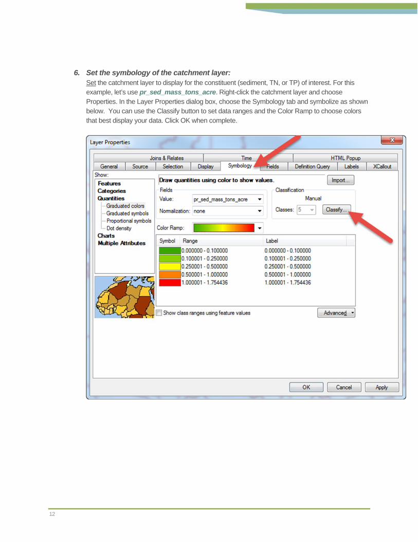
6. Set the symbology of the catchment layer: Set the catchment layer to display for the constituent (sediment, TN, or TP) of interest. For this example, let’s use pr_sed_mass_tons_acre. Right-click the catchment layer and choose Properties. In the Layer Properties dialog box, choose the Symbology tab and symbolize as shown below. You can use the Classify button to set data ranges and the Color Ramp to choose colors that best display your data. Click OK when complete.

13
Your data should now be displayed for use in source assessments, such as is shown below.

14
2.2 EVALUATE PRACTICE FEASIBILITY This section walks through an example of how to develop a map that could be used to evaluate the feasibility of placing practices on the landscape (Figure 3). This section covers an example of field-scale locations where PTMApp-Desktop outputs indicate practices are feasible in our workshop subwatershed.
Figure 3. Example of Practice Feasibility: Potential opportunities for BMPs and CPs found using PTMApp-Desktop within the Pomme de Terre River Watershed. BMPs and CPs are shown as either (A) structural or (B) non-structural practices.
A
B
15
2.2.1 HOW TO: EVALUATE PRACTICE FEASIBILITY
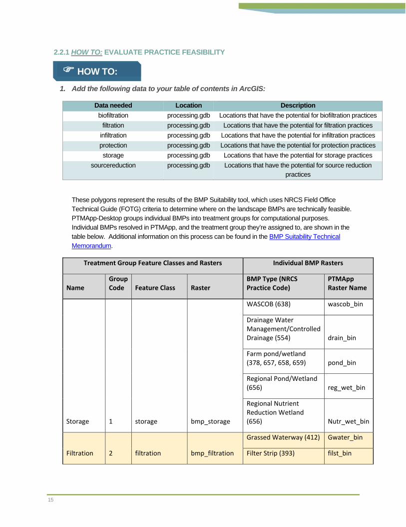
1. Add the following data to your table of contents in ArcGIS:
Data needed Location Description
biofiltration processing.gdb Locations that have the potential for biofiltration practices
filtration processing.gdb Locations that have the potential for filtration practices
infiltration processing.gdb Locations that have the potential for infiltration practices
protection processing.gdb Locations that have the potential for protection practices
storage processing.gdb Locations that have the potential for storage practices
sourcereduction processing.gdb Locations that have the potential for source reduction practices
These polygons represent the results of the BMP Suitability tool, which uses NRCS Field Office Technical Guide (FOTG) criteria to determine where on the landscape BMPs are technically feasible. PTMApp-Desktop groups individual BMPs into treatment groups for computational purposes. Individual BMPs resolved in PTMApp, and the treatment group they’re assigned to, are shown in the table below. Additional information on this process can be found in the BMP Suitability Technical Memorandum.
Treatment Group Feature Classes and Rasters Individual BMP Rasters
Name Group Code Feature Class Raster
BMP Type (NRCS Practice Code)
PTMApp Raster Name
Storage 1 storage bmp_storage
WASCOB (638) wascob_bin
Drainage Water Management/Controlled Drainage (554) drain_bin
Farm pond/wetland (378, 657, 658, 659) pond_bin
Regional Pond/Wetland (656) reg_wet_bin
Regional Nutrient Reduction Wetland (656) Nutr_wet_bin
Filtration 2 filtration bmp_filtration
Grassed Waterway (412) Gwater_bin
Filter Strip (393) filst_bin
HOW TO:

16
Treatment Group Feature Classes and Rasters Individual BMP Rasters
Name Group Code Feature Class Raster
BMP Type (NRCS Practice Code)
PTMApp Raster Name
Biofiltration 3 biofiltration bmp_biofilt
Denitrifying Bioreactor (605) Denit_bin
Saturated Buffer (604) SatBuff_bin
Infiltration 4 infiltration bmp_infiltration
Multi‐stage Ditch (N/A) ditch2s_bin
Infiltration Trench or Small Basin (N/A) InfTrench_bin
Protection 5 protection bmp_prot
Grade Stabilization (410) protect_bin
Grassed Waterway (412) Gwater_bin
Critical Planting Areas (342) crit_plant_bin
Shoreline Restoration/Protection (580) shore_bin
Source Reduction 6 sourcereduction bmp_sred
Cover Crops (340) CovCrop_bin
Perennial Crops (327) peren_bin
Nutrient Management of Groundwater for Nitrate (590) NO3_bin

17
2. Set the symbology: Set the symbology of the practice treatment groups to highlight areas on the map(s) where practices have the potential to be placed on the landscape. An example of which is shown below. Your data should now be set up to display locations where PTMApp-Desktop predicts BMPs are feasible.

18
2.3 ESTIMATE WATER QUALITY BENEFITS This section walks through an example of how to develop a map that displays the estimated water quality benefits of implementing practices in the workshop subwatershed. This section covers an example of the treatment cost for reducing sediment ($/mass/year) to the outlet of the workshop subwatershed. An example map displaying similar results from the Pomme de Terre River Watershed is shown below (Figure 4).
Figure 4. Example of water quality benefits estimation: The treatment cost (tons/dollar/year) of reducing sediment delivered to Planning Region outlets using Storage practices. Similar products can be developed for total nitrogen and total phosphorus.

19
2.3.1 HOW TO: ESTIMATE WATER QUALITY BENEFITS
1. Add the following data to your table of contents in ArcGIS:
Data needed Location Description
catchments processing.gdb Individual hydrologic catchment boundaries that average 40 acres in area
table_ca_bmp_costeff processing.gdb Table with BMP cost-effectiveness data for catchments, routed to priority resource locations
p_res_pts processing.gdb Point locations of priority resources and/or plan regions, with water quality goals in attributes. These were determined by user prior to running PTMApp-Desktop.
a. Attribute values used in this section:
Data Source Attribute Description catchments catch_ID Unique whole number ID for catchments
table_ca_bmp_costeff p_res_catch_ID Unique whole number ID for priority resource locations
grp_code BMP treatment group code (1-6)
CI_SQ_02 BMP cost index for sediment reduction (BMP cost [$]/ ton reduced) from 2-year, 24-hour event at a given priority resource point based upon median (Q2) effectiveness.
p_res_pts OBJECTID The OBJECT ID from the p_res_pts point layer is used to create the p_res_catch_ID
2. Identify the priority resource point (p_res_pts) where you’d like information about water quality benefits:
DESCRIPTION – This can be accomplished using the identify button ( ). The p_res_pts OBJECTID attribute is used to create the p_res_catch_ID in all PTMApp-Desktop output data. For this example, let’s use the workshop subwatershed outlet, OBJECITID: 3 (also p_res_catch_ID = 3). This is consistent with the Source Load Assessment step.
HOW TO:

20
STEPS – a. Select the Identify function and then click on the p_res_pts of interest and note the
OBJECTID. In our case we’re looking at the project outlet, OBJECTID = 3.
3. Open the table_ca_bmp_costeff attribute table and select by attribute: DESCRIPTION – Select records with “p_res_catch_ID = 3”. Note, each catchment can be associated with multiple treatment groups. You may also want to select data based on the treatment group that you’d like displayed. To do this, add an “AND” to your query statement and select your desired treatment group based on the “grp_code” attribute. The table below shows the description of the treatment groups associated with the different “grp_code” integer values. For this example, let’s include “grp_code= 6”.
grp_code Treatment Group
1 Storage
2 Filtration
3 Biofiltration
4 Infiltration
5 Protection
6 Source Reduction
21
STEPS –
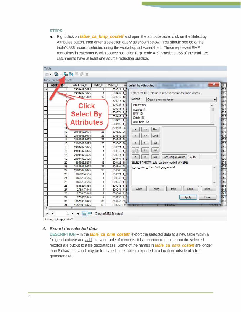
a. Right click on table_ca_bmp_costeff and open the attribute table, click on the Select by
Attributes button, then enter a selection query as shown below. You should see 66 of the table’s 838 records selected using the workshop subwatershed. These represent BMP reductions in catchments with source reduction (grp_code = 6) practices. 66 of the total 125 catchments have at least one source reduction practice.
4. Export the selected data:
DESCRIPTION – In the table_ca_bmp_costeff, export the selected data to a new table within a file geodatabase and add it to your table of contents. It is important to ensure that the selected records are output to a file geodatabase. Some of the names in table_ca_bmp_costeff are longer than 8 characters and may be truncated if the table is exported to a location outside of a file geodatabase.

22
STEPS – Select Export from the table options dropdown menu and, in the Export Data dialog box, save the Selected records to a file geodatabase.

23
5. Join the tables: DESCRIPTION – Join the table created in Step 4 to the catchment layer using the catch_ID as the join field for both data sources
STEPS – a. Right click on catchment and select Joins and Relates > Join b. Make sure catch_ID is selected for both the feature class and table join fields (#’s 1 and 3 in
Join Data dialog box) and that the exported table from the previous step is your join table (#2).

24
6. Set the symbology of the catchments layer: DESCRIPTION – Set the catchment layer to display for the constituent (sediment, TN, or TP) of interest. For this example, let’s use CI_SQ_02. Right-click the catchment layer and choose Properties. In the Layer Properties dialog box, choose the Symbology tab and symbolize as shown below. You can use the Classify button to set data ranges and the Color Ramp to choose colors that best display your data. You can also manually adjust how data are shown in your ArcMap Table of Contents under the ‘Label’ tab shown below. Click OK when complete.
This will display the cost index ($ spent/ton of sediment reduced) for treating sediment delivered to the priority resource and treatment group you selected. In our case, for Source Reduction practices (grp_code = 6) upstream of our project outlet (p_res_catch_id = 3). It is important to note that the default dollar values in this table are based on those run in the Cost Analysis module. By default, PTMApp-Desktop uses EQIP payments schedules for BMP costs, which represents the cost for installation only. As these values may not reflect the true cost of implementing a practice or project in your area, you may want to consider displaying your information on a high to low scale, rather than exact dollars. The scale to the right shows raw values, but you could (for example) label these as “Very Low”, “Low”, “Moderate”, “High”, and “Very High”. Your data should now be displayed for use in estimating water quality benefits.

25
2.4 TARGET PREFERRED PRACTICE LOCATIONS This section covers an example of how to use PTMApp-Desktop data to develop a list of targeted practices to use in implementation planning. The example below (Figure 5) is from the Pomme de Terre River Watershed and shows preferred practices for treating sediment and nutrients in the Middle Pomme de Terre River Watershed Planning Region. After completing this step, you should be able to develop your own implementation scenarios and process them through PTMApp-Desktop Treatment Trains analysis.
Figure 5. Example of conservation practice targeting: preferred locations for structural conservation practices in the Middle Pomme de Terre River Watershed Planning Region.

26
2.4.1 HOW TO: TARGET PREFERRED PRACTICE LOCATIONS
The following criteria were used for selecting practices for Targeting Preferred Practice Locations:
Only look at structural practices biofiltration, infiltration, protection, and storage. Cost-effectiveness to reduce sediment < $10,000/ton AND Cost-effectiveness to reduce TP <=
$10,000/lb as measured at the subwatershed outlet (p_res_catch_ID = 3). Sediment reductions from 2-year, 24-hour event > 1 ton AND TP reductions from 2-year, 24-
hour event > 1 lb as measured at the subwatershed outlet (p_res_catch_ID = 3).
1. To extract BMPs based on these criteria, add the following data to your table of contents in ArcGIS:
Data needed Location Description
biofiltration processing.gdb Locations that have the potential for biofiltration practices
filtration processing.gdb Locations that have the potential for filtration practices
infiltration processing.gdb Locations that have the potential for infiltration practices
protection processing.gdb Locations that have the potential for protection practices
sourcereduction processing.gdb Locations that have the potential for source reduction practices
storage processing.gdb Locations that have the potential for storage practices
table_ba_bmp_all processing.gdb Table containing benefits analysis for each BMP
table_ba_load_red processing.gdb Table containing BMP load reductions at priority resource locations.
a. Attribute values used in this section:
Data Source Attribute Description table_ba_bmp_all unq_BMP_ID Unique ID assigned to each BMP.
Concatenation of BMP_ID, Catch_ID, and grp_code.
table_ba_load_red p_res_catch_ID Unique whole number ID for priority resource locations
grp_code BMP treatment group code (1-6)
unq_BMP_ID Unique ID assigned to each BMP. Concatenation of BMP_ID, Catch_ID, and grp_code.
HOW TO:

27
Data Source Attribute Description R_SQ2_02 BMP sediment reduction (tons) from 2-year, 24-
hour event at a given priority resource point based upon median (Q2) effectiveness
R_PQ2_02 BMP total phosphorus reduction (tons) from 2-year, 24-hour event at a given priority resource point based upon median (Q2) effectiveness
p_res_pts OBJECTID The OBJECT ID from the p_res_pts point layer is used to create the p_res_catch_ID
2. Run the “Merge” operation on all BMP layers: DESCRIPTION – This will join the spatial distribution of all the potential practices. Be sure to save the output to a file geodatabase. Similar to early steps, saving outside of a file geodatabase could cause attribute names to be truncated.
STEPS – a. Select Data Management > General > Merge function from Arc Toolbox. Add the BMP
treatment groups using the Input Datasets dropdown and save the data to a file geodatabase. (saved as … WorkshopMaterials\Build_Products\S4_S5_Targeted_BMPs\ S4_S5_Targeted_BMPs.gdb\allbmps)
3. Attribute BMP costs: DESCRIPTION – BMP costs, calculated after running the Cost Analysis module, have been added as a field in table_ba_bmp_all. Join ‘allbmps’ with this table so we can use it to attribute our BMP shapefile to include BMP costs.
28
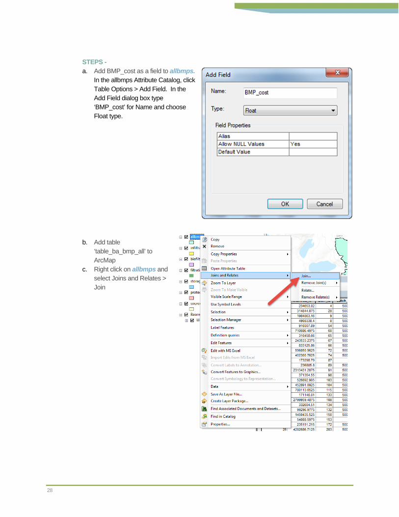
STEPS - a. Add BMP_cost as a field to allbmps.
In the allbmps Attribute Catalog, click Table Options > Add Field. In the Add Field dialog box type ‘BMP_cost’ for Name and choose Float type.
b. Add table
‘table_ba_bmp_all’ to ArcMap
c. Right click on allbmps and select Joins and Relates > Join
29
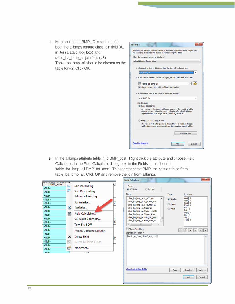
d. Make sure unq_BMP_ID is selected for
both the allbmps feature class join field (#1 in Join Data dialog box) and table_ba_bmp_all join field (#3). Table_ba_bmp_all should be chosen as the table for #2. Click OK.
e. In the allbmps attribute table, find BMP_cost. Right click the attribute and choose Field
Calculator. In the Field Calculator dialog box, in the Fields input, choose ‘table_ba_bmp_all.BMP_tot_cost’. This represent the BMP_tot_cost attribute from table_ba_bmp_all. Click OK and remove the join from allbmps.
30
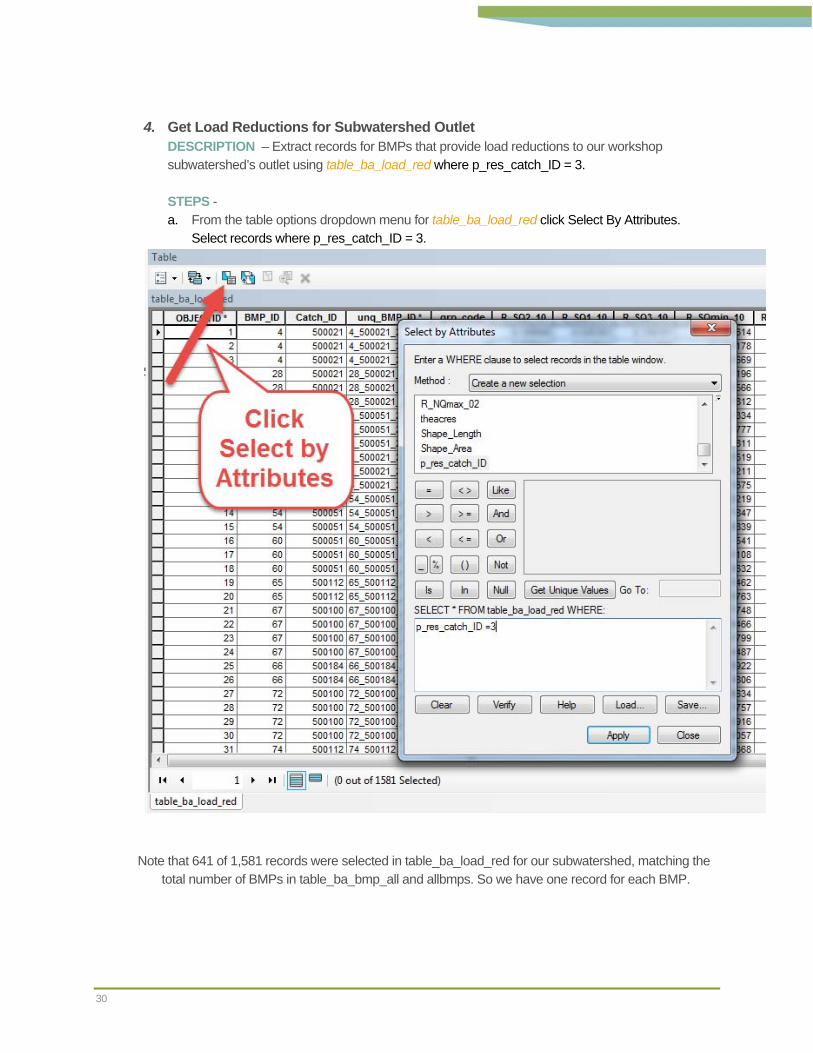
4. Get Load Reductions for Subwatershed Outlet DESCRIPTION – Extract records for BMPs that provide load reductions to our workshop subwatershed’s outlet using table_ba_load_red where p_res_catch_ID = 3. STEPS - a. From the table options dropdown menu for table_ba_load_red click Select By Attributes.
Select records where p_res_catch_ID = 3.
Note that 641 of 1,581 records were selected in table_ba_load_red for our subwatershed, matching the total number of BMPs in table_ba_bmp_all and allbmps. So we have one record for each BMP.
31
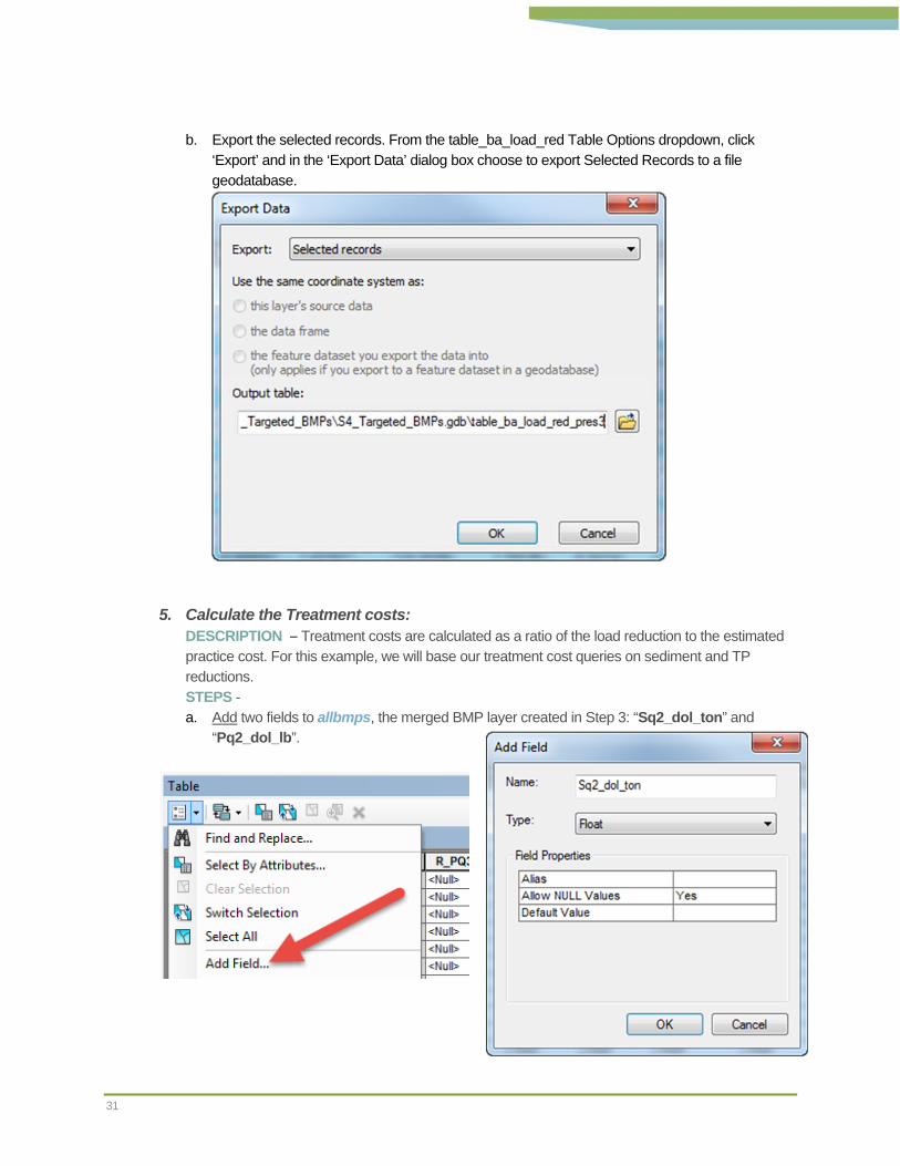
b. Export the selected records. From the table_ba_load_red Table Options dropdown, click ‘Export’ and in the ‘Export Data’ dialog box choose to export Selected Records to a file geodatabase.
5. Calculate the Treatment costs: DESCRIPTION – Treatment costs are calculated as a ratio of the load reduction to the estimated practice cost. For this example, we will base our treatment cost queries on sediment and TP reductions. STEPS - a. Add two fields to allbmps, the merged BMP layer created in Step 3: “Sq2_dol_ton” and
“Pq2_dol_lb”.

32
b. Join the table created in the previous step (table_ba_load_red_pres3) to the merged BMP file, allbmps, using the unq_bmp_ID.

33
c. Use the field calculator to set Sq2_dol_ton = “BMP_cost / R_SQ2_02” and Pq2_dol_lb = “BMP_cost / R_PQ2_02”. Note that since allbmps is joined to our exported table, the attribute fields will include their shapefile names (as shown below).
Note: We’ve used the median reductions in sediment and TP based on a 2-year, 24-hour discharge event.

34
6. Select Preferred Practices:
DESCRIPTION – Use the select by attributes feature to select the records which fit our selection criteria. You can choose any of a number of criteria, including total reductions or cost-effectiveness to reduce sediment, TP, and TN as well as BMP treatment group, footprint (square-feet), drainage area (acres), or cost among others. For this example, we’ll use the following: Only look at structural practices biofiltration, infiltration, protection, and storage treatment
groups. Cost-effectiveness to reduce sediment <= $10,000/ton AND Cost-effectiveness to reduce TP
<= $10,000/lb as measured at the subwatershed outlet (p_res_catch_ID = 3). Sediment reductions from 2-year, 24-hour event > 1 ton AND TP reductions from 2-year, 24-
hour event > 1 lb as measured at the subwatershed outlet (p_res_catch_ID = 3).
STEPS – a. Your query statement should be: “allbmps.grp_code <> 2 AND allbmps.grp_code <> 6
AND allbmps.Sq2_dol_ton <=10000 AND allbmps.Pq2_dol_lb <=10000 AND table_ba_load_red_pres3.R_SQ2_02 >1 AND table_ba_load_red_pres3.R_PQ2_02 >1”

35
b. Export the selected features to a file geodatabase. Right-click allbmps and navigate to Data > Export Data
c. Be sure to save the output to a file geodatabase. Similar to early steps, saving outside of a file geodatabase could cause attribute names to be truncated.
d. For the workshop materials, 60 BMPs met the criteria set in the previous step and were included in the exported shapefile.

36
7. Run Treatment Trains: DESCRIPTION – Your layer, exported in Step 6, should be ready to input into the Treatment Trains tool. For simplicity, a smaller subset of the targeted BMPs was included with the workshop materials titled ‘BMPs_For_TT’. This includes seven BMPs that might be considered as part of a grant application and/or your first round on implementation in the subwatershed. These were the better performing BMPs within each treatment group. Use this feature class to run treatment trains as shown below. For additional information on treatment trains, see Workshop Section 2. Note: Apply Lakes should be checked if Lake Routing was run for your analysis.

37
2.5 DEVELOP TARGETED IMPLMENTATION PLAN This section describes examples of the types of secondary data, not generated by PTMApp-Desktop, which could be used to finalize the list of practices considered for a Targeted Implementation Plan.
Previous steps described in this manual have relied exclusively on the data output from PTMApp-Desktop. However, a multitude of additional data and information can be used to help target practice locations for consideration in your implementation plan. For example, local knowledge could be used to exclude areas that lack landowners who are willing to implement additional conservation practices. The results of other analyzes, such as Zonation, could also be used to target practices in locations that provide multiple benefits in addition to water quality improvements.
PTMApp-Desktop users are encouraged to integrate and document the use of these external data sources, where applicable, when developing Targeted Implementation Plans.

38
2.6 ESTIMATE BENEFITS OF TARGETED IMPLMENTATON PLAN This section walks through an example of how to develop a map that displays the water quality benefits (i.e. load reductions) associated with a Targeted Implementation Plan. This section shows how to use PTMApp-Desktop data to build the summary table and figures, such as in Figure 6, which shows an example implementation table with the “best” structural practices to begin implementation in the Middle Pomme de Terre River Watershed Planning Region.
Figure 6. Example of a Targeted Implementation Plan: A table of the 10 “best” structural practices in the Middle Pomme de Terre River Watershed Planning Region.

39
2.6.1 HOW TO: BENEFITS OF TARGETED IMPLMENTATON PLAN
1. Export Results to Excel: DESCRIPTION – After treatment trains has finished running, add the tables below to your ArcMap table of contents. Then export the data to a .csv file. For this example, let’s focus exclusively on the “table_treat_train_p_res” table.
Data needed Location Description
table_treat_train_catch processing.gdb Table with results of treatment train analysis. Loads are relative to catchment outlet.
table_treat_train_p_res processing.gdb Table with results of treatment train analysis. Loads are relative to priority resource catchment outlets (i.e. the resource points).
p_res_catchment processing.gdb Priority resource hydrologic catchment boundaries and/or plan regions.
a. Attribute values used in this section:
Data Source Attribute Description table_treat_train_p_res p_res_catch_ID Unique whole number ID for priority resource locations
Lred_R_SQ2_02 BMP sediment reduction (tons) at a given priority resource point from a 2-year, 24-hour event based upon median effectiveness of BMPs in user-defined shapefile.
Lred_R_PQ2_02 BMP total phosphorus reduction (lbs) at a given priority resource point from a 2-year, 24-hour event based upon median effectiveness of BMPs in user-defined shapefile.
Lred_R_NQ2_02 BMP total nitrogen reduction (lbs) at a given priority resource point from a 2-year, 24-hour event based upon median effectiveness of BMPs in user-defined shapefile.
p_res_catch_ID Unique whole number ID for priority resource catchment
p_res_catchment p_res_catch_ID Unique whole number ID for priority resource catchment
HOW TO:
40
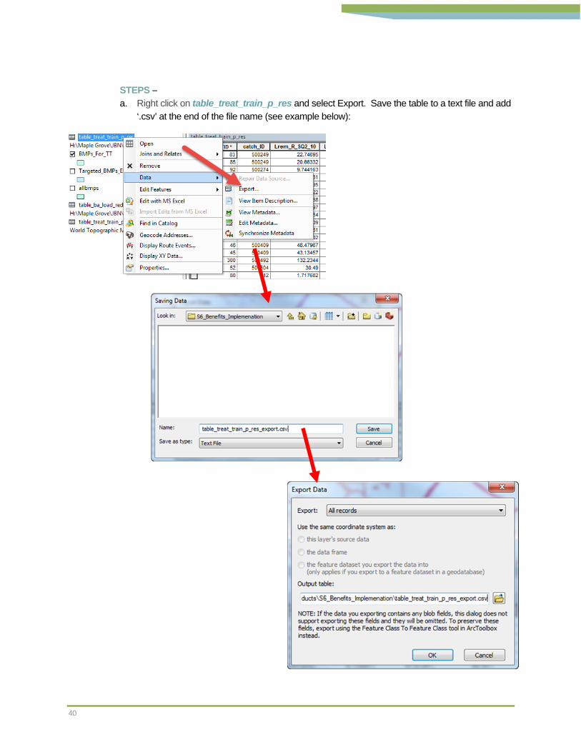
STEPS – a. Right click on table_treat_train_p_res and select Export. Save the table to a text file and add
‘.csv’ at the end of the file name (see example below):
41
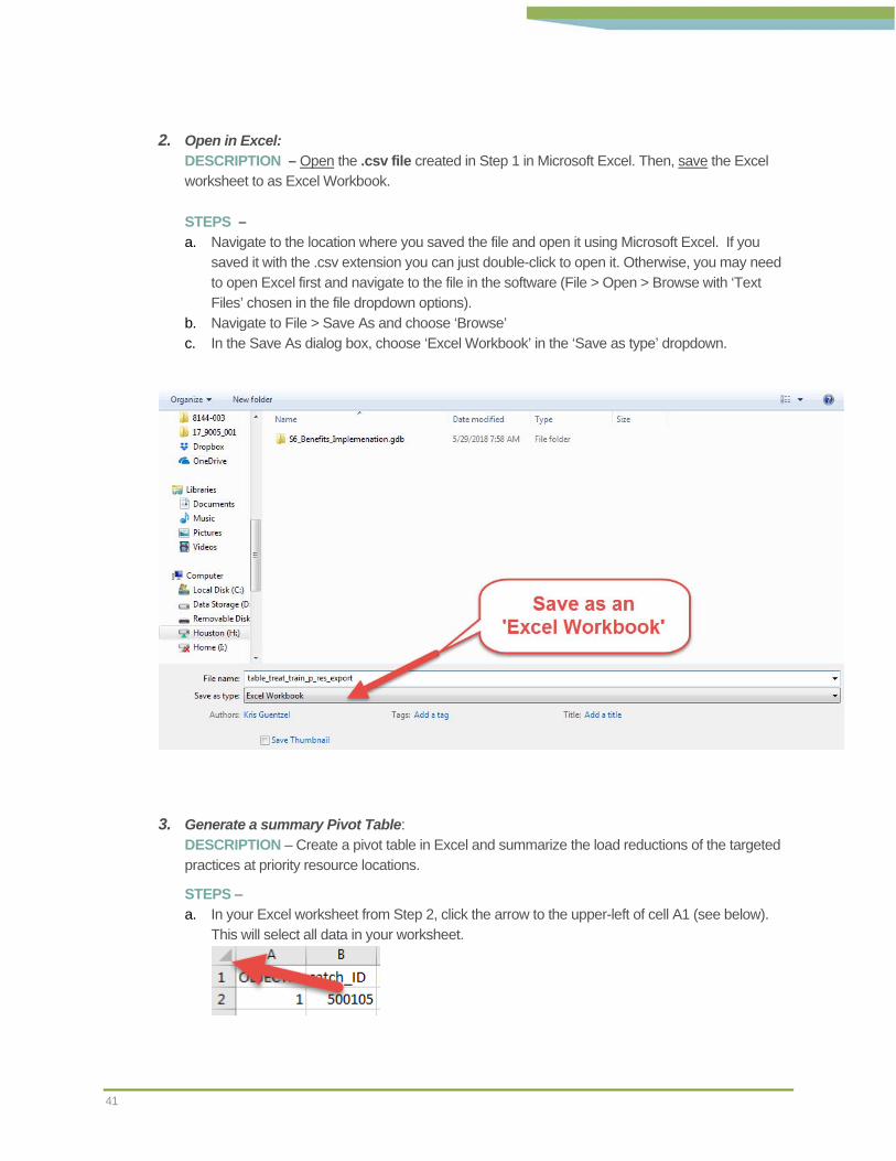
2. Open in Excel: DESCRIPTION – Open the .csv file created in Step 1 in Microsoft Excel. Then, save the Excel worksheet to as Excel Workbook.
STEPS – a. Navigate to the location where you saved the file and open it using Microsoft Excel. If you
saved it with the .csv extension you can just double-click to open it. Otherwise, you may need to open Excel first and navigate to the file in the software (File > Open > Browse with ‘Text Files’ chosen in the file dropdown options).
b. Navigate to File > Save As and choose ‘Browse’ c. In the Save As dialog box, choose ‘Excel Workbook’ in the ‘Save as type’ dropdown.
3. Generate a summary Pivot Table: DESCRIPTION – Create a pivot table in Excel and summarize the load reductions of the targeted practices at priority resource locations.
STEPS – a. In your Excel worksheet from Step 2, click the arrow to the upper-left of cell A1 (see below).
This will select all data in your worksheet.

42
b. Click on the “INSERT” ribbon and select “Pivot Table” and save the output to a new worksheet within your Excel document.
c. Click on each of the following attributes in the Pivot Table Fields i. Lred_R_SQ2_02 ii. Lred_R_PQ2_02 iii. Lred_R_NQ2_02 iv. p_res_catch_ID
d. Drag each ‘Lred…’ attribute into the ‘Values’ box. If ‘Sum of’ isn’t chosen as the default way to summarize ‘Lred’ values, you can change it by right-clicking items in the ‘Values’ box and selecting Value Field Settings > Sum.
e. Drag p_res_catch_ID into the ‘Rows’ box.

43
4. View load reductions at Priority Resource Points DESCRIPTION –This step will provide you the total load reductions to each priority resource location that was inserted at the start of running PTMApp-Desktop. The same information could be summarized at different spatial scales (i.e. catchments).
Note: Priority resource points 1 and 4 had received no treatment from BMPs in the ‘BMPs_for_TT’
implementation shapefile. Although there are reduction values shown for resource point 1, they represent rounding errors in the tool and are effectively ‘0’.

44
2.7 ASSESS FEASIBILITY OF MEASURABLE GOALS Briefly, this process should involve comparing your anticipated benefits and investments (time, money, etc.) towards implementing your Targeted Implementation Plan and your resource goals to assess if attaining the goals is feasible through your targeted implementation plan.
The results of a Targeted Implementation Plan described in Section 2.6, should be evaluated to determine if they are feasible to achieve and if they are sufficient to reach local management goals. If a scenario developed through this workflow is not feasible, simply loop back through and develop a new targeted scenario.
3 CONCLUSIONS
This workshop manual was developed with the purpose of demonstrating how the PTMApp-Desktop outputs could be used to develop a Targeted Implementation Plan. The intended outcome is to empower local governmental units (LGU), who have completed processing data with PTMApp-Desktop, to be able to utilize the data on their own without the need for external consultation. This should position LGUs to utilize PTMApp-Desktop to develop implementation plans that are prioritized, targeted, and result in measurable water quality improvements.