Session will begin @ 10:00 AM (Pacific Day Time)€¦ · Stress Life –Variable Amplitude •For an irregular load history –Cycle counting for irregular load histories is done

FRACTURE MECHANICS IN ANSYS R16Session will begin @ 10:00 AM (Pacific Day Time)

• If you will be connected to audio using your

computer’s microphone and speakers (VoIP).

A headset is recommended.

• Or, you may select Use Telephone after

joining the Webinar.

Welcome to the Webinar. Please make sure your audio is working

Feel free to use computer speakers or telephone

Type any questions you have here

1

Ozen Engineering Inc.

1210 E. Arques Ave, Suite 207

Sunnyvale, CA 94085

[email protected]

Fracture Mechanics in Ansys R16

Session-05

Fatigue Crack Propagation

Fatigue Overview

• Fatigue is divided into two sub-sections:– High-cycle fatigue (stress-life)

• Number of load cycles high 1e5 to 1e9

• Lower stresses wrt ultimate strength

– Low-cycle fatigue (strain-life)• Number of load cycle low <=1e5

• Plastic deformation is present (ie stresses over yield strength)

3

Fatigue Overview

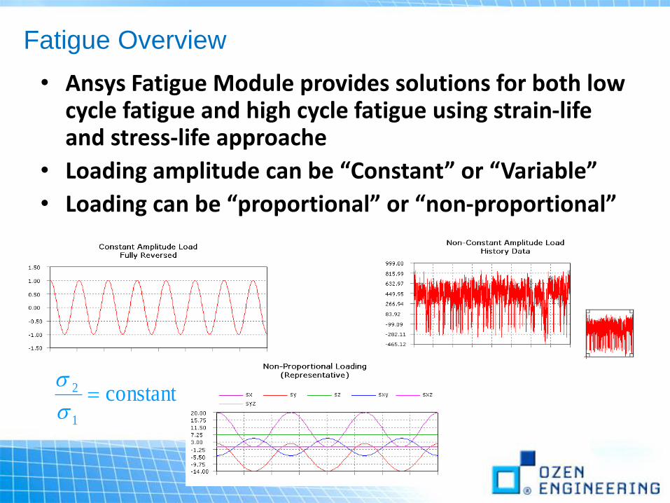
• Ansys Fatigue Module provides solutions for both low cycle fatigue and high cycle fatigue using strain-life and stress-life approache

• Loading amplitude can be “Constant” or “Variable”

• Loading can be “proportional” or “non-proportional”

4

constant1

2

Fatigue Overview

• Some critical definitions based on min and max stress values:– Stress range : Smax-Smin

– Mean stress: (Smax+Smin)/2

– Stress amplitude/alternating stress: (Smax-Smin)/2

– Stress ratio R: Smin/Smax

– Fully-reversed loading (mean stress = 0, R=-1)

– Zero-based loading (mean stress = Smax/2, R=0)

5

STRESS-LIFE

HIGH CYCLE FATIGUE

6

Stress Life

• Fatigue analysis is based on a linear static analysis assumption (still can do fatigue calculations on a nonlinear system but with caution)

• Fatigue analysis requires only two additional steps over a standard structural analysis

– Material properties (S-N curves)

– Post-processing using the Fatigue Tool

7

Stress Life

• Loading to fatigue failure relation is given by a Stress-Life (S-N) curve

8

Linear Plot Logarithmic Plot

The same data is shown here with both a linear and logarithmic plot. Because of the

nature of the data, it is often easier to use a logarithmic plot to view the S-N curve.

Stress Life

• Contact Regions– Regions with linear contact (bonded or no-

separation) can be included in “constant amplitude, proportional loading”

– For Nonlinear contact, one should use “constant amplitude, non-proportional loading”

• Loads and Supports– Bearing Load (direction of load does not reverse)

– Bolt Load (2 step analysis)

– Compression only support (nonlinear only in one direction, effectively frictionless contact)

9

Stress Life

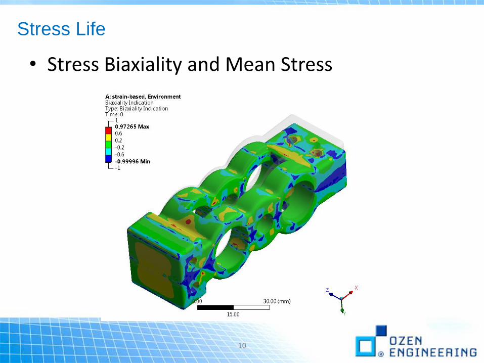
• Stress Biaxiality and Mean Stress

10

Stress Life

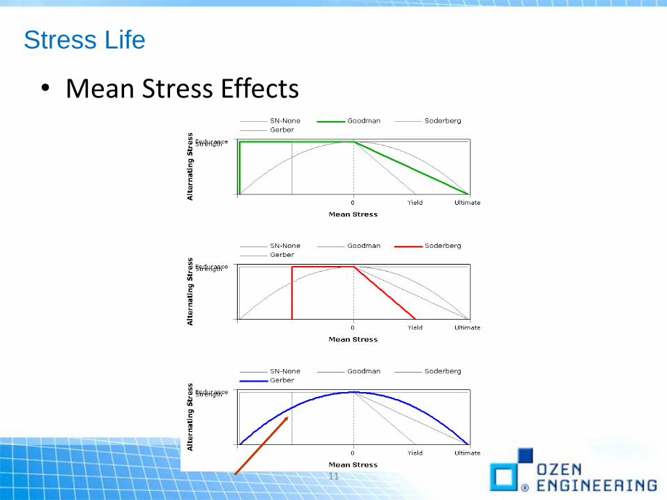
• Mean Stress Effects

11

Stress Life

• Other factors affecting S-N curve can be taken into account via what’s called “Strength Factor”

12

Stress Life

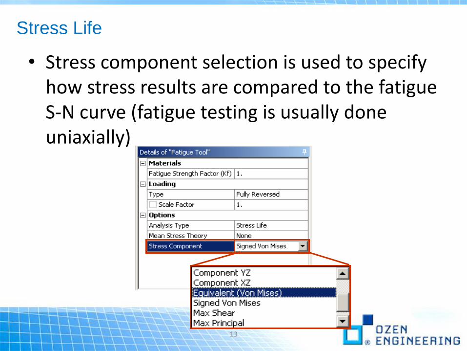
• Stress component selection is used to specify how stress results are compared to the fatigue S-N curve (fatigue testing is usually done uniaxially)

13

Stress Life – Constant Amplitude

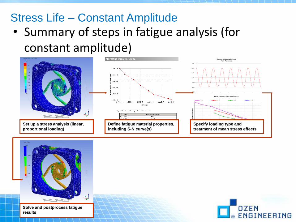
• Summary of steps in fatigue analysis (for constant amplitude)

Set up a stress analysis (linear,

proportional loading)

Solve and postprocess fatigue

results

Define fatigue material properties,

including S-N curve(s)

Specify loading type and

treatment of mean stress effects

Stress Life – Variable Amplitude

• For an irregular load history

– Cycle counting for irregular load histories is done with a method called rainflowcycle counting

• Rainflow cycle counting is a techniquedeveloped to convert an irregular stresshistory (sample shown on right) to cycles used for fatigue calculations

• Cycles of different mean stress (“mean”)and stress amplitude (“range”) are counted. Then, fatigue calculations are performed using this set of rainflow cycles.

time

1fi

i

N

N


– Arbitrary load history can be divided into a matrix (“bins”) of different cycles of various mean and range values

– After a fatigue analysis is performed, the amount of damage each “bin” (cycle) caused can be plotted

• For each bin from the rainflow matrix, the amount of life used up is shown (percentage)

• Per Miner’s rule, if the damage sums to 1 (100%), failure will occur.


• Summary of steps for variable amplitude case:

Set up a stress analysis (linear,

proportional loading)

Specify number of bins for

rainflow cycle counting

Define fatigue material properties,

including S-N curve(s)

Specify loading history data and

treatment of mean stress effects

Solve and review fatigue results, (e.g., damage matrix, damage contour,

life contour, etc.)

• In constant amplitude loading, if stresses are lower than the lowest limit defined on the S-N curve, recall that the last-defined cycle will be used. However, in variable amplitude loading, the load history will be divided into “bins” of various mean stresses and stress amplitudes. Since damage is cumulative, these small stresses may cause some considerable effects, even if the number of cycles is high. Hence, an “Infinite Life” value can also be input in the Details view of the Fatigue Tool to define what value of number of cycles will be used if the stress amplitude is lower than the lowest point on the S-N curve.– Recall that damage is defined as the ratio of cycles/(cycles to failure), so for small stresses with

no number of cycles to failure on the S-N curve, the “Infinite Life” provides this value.– By setting a larger value for “Infinite Life,” the effect of the cycles with small stress amplitude

(“Range”) will be less damaging since the damage ratio will be smaller.


• The “Bin Size” can also be specified in the Details view of the Fatigue Tool for the load history

– The size of the rainflow matrix will be bin_size x bin_size.

– The larger the bin size, the bigger the sorting matrix, so the mean and range can be more accurately accounted for. Otherwise, more cycles will be put together in a given bin (see graph on bottom).

– However, the larger the bin size, the more memory and CPU cost will be required for the fatigue analysis.

Bin Size=10 Bin Size=32 Bin Size=64

The bin size can range from 10 to 200. The default value is

32, and it can be changed in the Control Panel.


• Results similar to constant amplitude cases are available:

• Instead of the number of cycles to failure, Life results report the number of loading ‘blocks’ until failure. For example, if the load history data represents a given ‘block’ of time – say, one week – and the minimum life reported is 50, then the life of the part is 50 ‘blocks’ or, in this case, 50 weeks.

• Damage and Safety Factor are based on a Design Life input in the Details view, but these are also ‘blocks’ instead of cycles.

• Biaxiality Indication is the same as the constant amplitude case and is available for variable amplitude loading.

• Equivalent Alternating Stress is not available as output for the variable amplitude case. This is because a single value is not used to determine cycles to failure. Instead, multiple values are used, based on the loading history.

• Fatigue Sensitivity is also available for the ‘blocks’ of life.


• The idea here is that instead of using a single loading environment, two loading environments will be used for fatigue calculations.

• Instead of using a stress ratio, the stress values of the two loading environments will determine the min and max values. This is why this method is called non-proportional since one set of stress results is not scaled, but two are used instead.

• Because two solutions are required, the use of the Solution Combination branch makes this possible.

Stress Life – Constant Amplitude & Non-Proportional

• The procedure for the constant amplitude, non-proportional case is the same as the one for the constant amplitude, proportional loading situation with the following exceptions:

1. Set up two Environment branches with different loading conditions

2. Add a Solution Combination branch and specify the two Environments to use

3. Add the Fatigue Tool (and any other results) for the Solution Combination branch, and specify “Non-Proportional” for the loading Type.

4. Request fatigue results as normal and solve


1. Set up two loading environments:

• These two loading environments can have two distinct sets of loads (supports should be the same) to mimic alternating between two loads– An example is having one bending load and one torsional load for the two

Environments. The resulting fatigue calculations will assume an alternating load between the two.

• An alternating load can be superimposed on a static load– An example is having a constant pressure and a moment load. For one

Environment, specify the constant pressure only. For the other Environment, specify the constant pressure and the moment load. This will mimic a constant pressure and alternating moment.

• Use of nonlinear supports/contact or non-proportional loads– An example is having a Compression Only support. As long as rigid-body

motion is prevented, the two Environments should reflect the loading in one and the opposite direction.


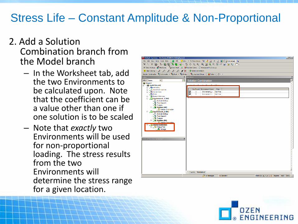
2. Add a Solution Combination branch from the Model branch– In the Worksheet tab, add

the two Environments to be calculated upon. Note that the coefficient can be a value other than one if one solution is to be scaled

– Note that exactly two Environments will be used for non-proportional loading. The stress results from the two Environments will determine the stress range for a given location.


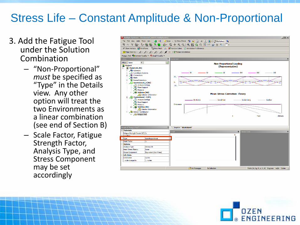
3. Add the Fatigue Tool under the Solution Combination– “Non-Proportional”

must be specified as “Type” in the Details view. Any other option will treat the two Environments as a linear combination (see end of Section B)

– Scale Factor, Fatigue Strength Factor, Analysis Type, and Stress Component may be set accordingly


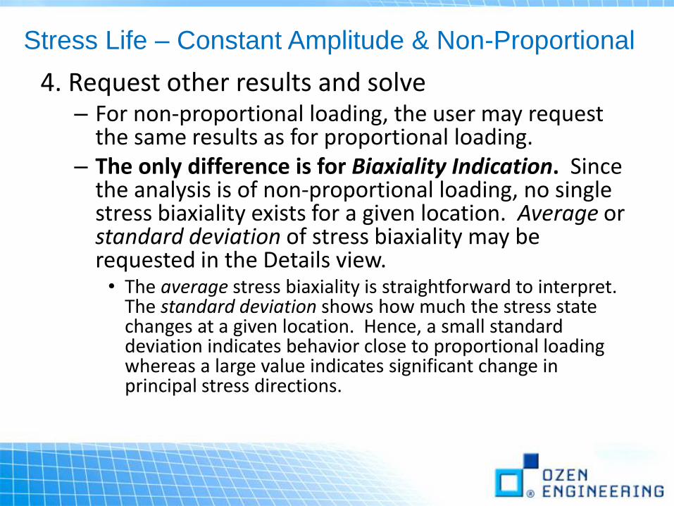
4. Request other results and solve– For non-proportional loading, the user may request

the same results as for proportional loading.– The only difference is for Biaxiality Indication. Since

the analysis is of non-proportional loading, no single stress biaxiality exists for a given location. Average or standard deviation of stress biaxiality may be requested in the Details view.

• The average stress biaxiality is straightforward to interpret. The standard deviation shows how much the stress state changes at a given location. Hence, a small standard deviation indicates behavior close to proportional loading whereas a large value indicates significant change in principal stress directions.


STRAIN-LIFE

LOW CYCLE FATIGUE

27

• The Strain-Life Approach considers plastic deformation, and it is often used for low-cycle fatigue analyses.

• Similar to the existing stress-life approach, all relevant options and post-processing are specified with the addition of a “Fatigue Tool” object under the “Solution” branch

• The Strain-Life Approach supports the case of constant amplitude, proportional loading only.

Strain Life

• Steps in blue italics are specific to a stress analysis with the inclusion of the Fatigue Tool for the Strain-Life Approach:

• Attach Geometry• Assign Material Properties, including e-N Data• Define Contact Regions (if applicable)• Define Mesh Controls (optional)• Include Loads and Supports• Request Results, including the Fatigue Tool• Solve the Model• Review Results

Strain Life

• Unlike the stress-life approach, the strain-life approach considers the effect of plasticity. The equation relating total strain amplitude ea and life (Nf) is as follows:

where’f is the “Strength Coefficient”

b is the “Strength Exponent”

e’f is the “Ductility Coefficient”

c is the “Ductility Exponent”

• The graph on the right represents the equationgraphically when plotted on log-scale

• The blue segment is the elastic portion (first term), where b is the slope and ’f/E is the y-intercept

• The red segment is the effect of plasticity (second term) with c being the slope and e’f the y-intercept

• The green line shows the sum of the elastic and plastic portions

cff

b

f

f

a NNE

22 e

e

Strain Life

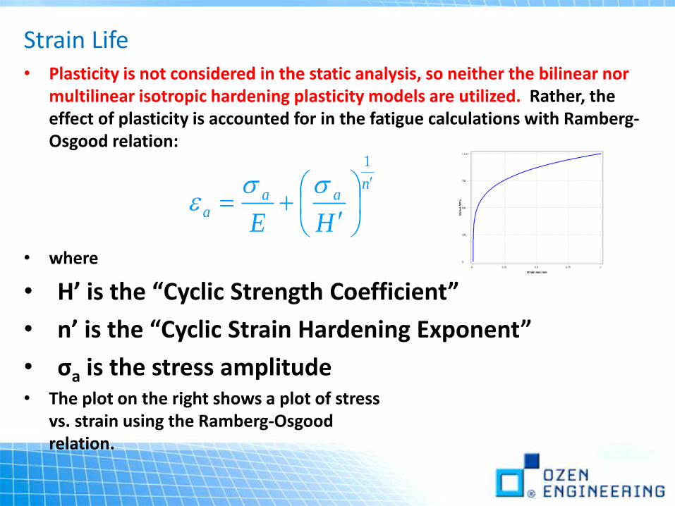
• Plasticity is not considered in the static analysis, so neither the bilinear nor multilinear isotropic hardening plasticity models are utilized. Rather, the effect of plasticity is accounted for in the fatigue calculations with Ramberg-Osgood relation:

• where

• H’ is the “Cyclic Strength Coefficient”

• n’ is the “Cyclic Strain Hardening Exponent”

• σa is the stress amplitude• The plot on the right shows a plot of stress

vs. strain using the Ramberg-Osgoodrelation.

naa

aHE

1

e

Strain Life

• Input of strain-life fatigue properties is done in the Engineering Data tab:

– “Young’s Modulus” E is input as normal

– “Strength Coefficient,” “Strength Exponent,” “Ductility Coefficient,” “Ductility Exponent,” “Cyclic Strength Coefficient,” and “Cyclic Strain Hardening Exponent” are strain-life input

Strain Life

• As noted earlier, constant amplitude, proportional loading is supported with the strain-life approach. After adding the “Fatigue Tool” object under the “Solution” branch, the Details view allows setting fatigue calculation options:– “Type” can be “Zero-Based” (0 to 2a), “Fully

Reversed” (-a to a), or a specified “Ratio”– The “Fatigue Strength Factor (Kf)” and “Scale

Factor” are similar to the stress-based approach.– The effect of mean stresses can be accounted

for under “Mean Stress Theory” (discussed next)– The “Stress Component” specified is used in

the fatigue calculations– “Infinite Life” simply defines the highest value

of life for easier viewing of contour plots, as the strain-life method has no built-in limits

Strain Life

• If the user wishes to use mean stress correction, there are two options available:

• “Morrow” modifies the elastic term as follows:

where m is the mean stress.

• The figure on the bottom illustrates the fact that the Morrow equation only modifies the elastic term

• Similar to the Goodman case for stress-life approach, compressive mean stresses are not assumed to have a positive effect on life

cff

b

f

f

mf

a NNE

21 e

e

Strain Life

• “SWT” (Smith, Watson, Topper) uses a different approach:

where max =m + a.– In this case, life is assumed to be related to the

product maxea

– The graph on the bottom shows the effect of both tensile and compressive mean stresses on life

cb

fff

b

f

f

a NNE

2

2

2

max e

e

Strain Life

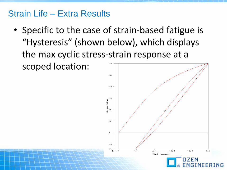
• Specific to the case of strain-based fatigue is “Hysteresis” (shown below), which displays the max cyclic stress-strain response at a scoped location:

Strain Life – Extra Results

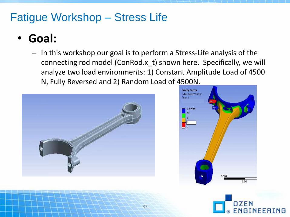
Fatigue Workshop – Stress Life

• Goal: – In this workshop our goal is to perform a Stress-Life analysis of the

connecting rod model (ConRod.x_t) shown here. Specifically, we will analyze two load environments: 1) Constant Amplitude Load of 4500 N, Fully Reversed and 2) Random Load of 4500N.

37

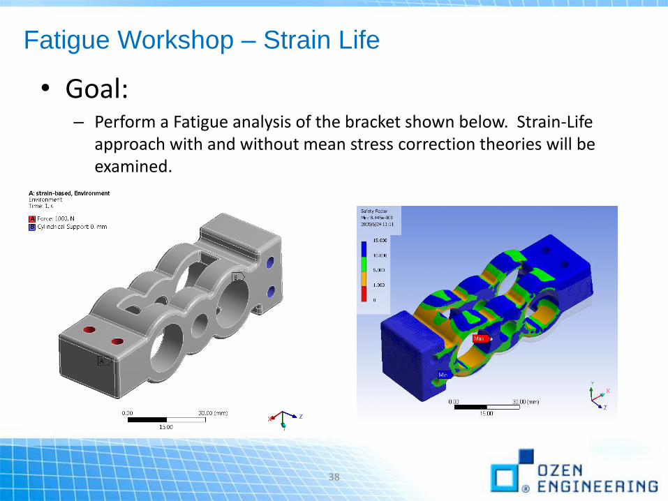
Fatigue Workshop – Strain Life

• Goal: – Perform a Fatigue analysis of the bracket shown below. Strain-Life

approach with and without mean stress correction theories will be examined.

38

END

Thanks for your attention !!!

Questions ?

CONTACT:

Attention: Can Ozcan ([email protected])OZEN ENGINEERING, INC.

1210 E. ARQUES AVE. SUITE: 207

SUNNYVALE, CA 94085

(408) 732-4665

[email protected]

www.ozeninc.com

mailto:[email protected]

http://www.ozeninc.com/

Documents

Session will begin @ 10:00 AM (Pacific Day Time)€¦ · Stress Life –Variable Amplitude •For an irregular load history –Cycle counting for irregular load histories is done