Session 12: Equilibrator-based surface measurements

Session 12: Equilibrator-based surface measurements

Gregor [email protected]

Overview– Basic Principle– How it started

• Weiss et al. 1981 and the NOAA SetUp during the SAGA II experiment • Current surface trace gas data – what happened?• NDIR and the GO-system

– CEAS- instruments – opening the field• Basics of functioning• The main players (if you were to buy an instrument) ….• … and how they work (CEAS, CRDS, oa-ICOS; and OF-CEAS)• Examples of gases (and isotopes) to be measured• Ocean community problems ….

– Matrix effects

• Some data from the field2

Overview

Overview II– Some often forgotten issues of equilibrator based measurements

• It is not in equilibrium (never, really)• Response time and equilibrator design• The total gas tension assumption

3

Overview

The Basic principle • Permanently renewed seawater supply

• Recirculating stream of air • Both phases “meet” in a vessel

designed to stimulate rapid gas-water exchange, usually in a counter-flow set-up

• In most case the equilibration vessel is open to the atmosphere, in a setting minimizing contamination by outside air.

• In gas stream analytical device to detect at least one gas species

• Air pressure, salinity , Tinsitu and Tequito be known

• Water vapour content to be known at point of measurement4

Basics

From Gülzow et al., 2011

The Basic principle • Actual measurement: mole fraction of the gas (i) in the gas phase (xi)

• Usually calculation of xi(dry)

• Correction for xi in situ considering changes in solubility due to T-change and assuming 100% water vapor saturation in the exchange vessel

5

Basics

From Gülzow et al., 2011

Takahashi et al., 1993

How it startedRay Weiss et al. 1981Weiss, R.F., 1981. Determinations of carbon dioxideand methane by Dual Catalyst Flame Ionisation Chromatography and nitrous oxide by Electron Capture Chromatography. J. Chrom. Sci. 19, 611-616.

James (Jim) Butler et al. The SAGA II Report (second Soviet-American Gas and Aerosol Experiment; SAGA II)“Five trace gases in the surface water and atmosphere of the West Pacific and East Indian Oceans were measured by automated gas chromatography from May through July 1987”

6

Somehistory

Butler et al., 1988

„The main question we needed to addresswas whether the equilibrator atmosphereproperly represented gas concentrations in the incoming water. We approached thisproblem by conducting some controlledexperiments in the laboratory and applyingthe results to a mass-balance model of theequilibrator, expressed in both differential and finite-increment form. Our objectiveswere to determine (1) the exit coefficient(piston velocity) and the rate constants forgas transfer within the equilibrator, (2) themaximum concentration of gas in theequilibrator atmosphere under steady-stateconditions, (3) the time required forequilibration, and (4) how much theconcentration of gas in the water dropsduring normal sampling. “

„The third GC (not shown) was essentially a Weiss GC configured onlyfor CO2 and CH4“

Somehistory

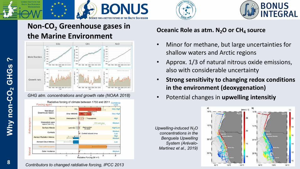
Non-CO2 Greenhouse gases in the Marine Environment

Oceanic Role as atm. N2O or CH4 source

• Minor for methane, but large uncertainties for shallow waters and Arctic regions

• Approx. 1/3 of natural nitrous oxide emissions, also with considerable uncertainty

• Strong sensitivity to changing redox conditions in the environment (deoxygenation)

• Potential changes in upwelling intensitiy

8

Why

non-

CO

2G

HG

s ?

GHG atm. concentrations and growth rate (NOAA 2018)

Contributors to changed ratdiative forcing, IPCC 2013

Upwelling-induced N2O concentrations in theBenguela Upwelling

System (Arévalo-Martinez et al., 2019)

The global data sets• Methane and nitrous oxide in the

MEMENTO data base (the MarinEMethanE and NiTrous Oxide database)

9

CH4 > 30,000 data entries

Status 2019Surface Measurements (Sampling Depth <10m)

Depth profiles (Sampling Depth > 10m)

N2O > 120,000 data entries

Dat

a G

aps

The global data sets

fCO2 in theSOCATdatabase

10

CO2 > 23.4 Miodata entries(2018)

Wealthofdata

Wea

lthof

data

–st

ill D

ata

Gap

s

11

What made the difference?

• Strong “science pull” driven by the awareness of the oceanic role as a carbon dioxide sink (1st IPCC Report in 1990)

• Non-consuming ideally suited instrument for CO2

LICOR 6251 in 1988, LI-6262 in 1990Wanninkhof et al., 1993, Goyet and Peltzer 1994

• Development of the GO-System as state-of-the art complete system

(Craig tells the history)

12

ND

IR a

ndG

O

Reaching out for other gases

13

Cavityenhancedopticaldetectors

Cavity enhanced absorption spectroscopy

Lambert Beer Law

With I the light intensity after passing the medium, I0 theinitial light intensity, s the absorbers`s cross section, L theoptical pathlength and N the number of absorbing molecules

CEAS use laser pumped cavity to enhance theoptical pathlength and better tuning of absorptionwavelengths.

CRDS

Oa-ICOS

OF-CEAS

???

14

Cavityenhancedopticaldetectors

Cavity enhanced absorption spectroscopy

• ALL work with tunable lasers and fulfill absorption or ring-down experiments over a range of wavelengths.

• ALL work at reduced pressure and stable temperature, and detect water vapor to deal with peak broadening.

• Off-axis Integrated Cavity Output Spectroscopy (oa-ICOS) and optical feedback-cavity enhanced absorption spectroscopy (OF-CEAS) both measure absorption through transmission; CRDS does not.

• Cavity ringdown spectroscopy (CRDS) and OF-CEAS work on locked laser modes, oa-ICOS does not.

CRDS

OA-ICOS

OF-CEAS

???


Cavity Ring Down Spectroscopy • Measures “decay” of a loaded resonator, and derives concentration from the decay time (or the decay time with absorber in relation to the decay time without absorber)

• Reality: tunable laser allows measurement in non absorbing wavelengh window, rather than without absorber15

CRDS

a is the absorption coefficient, σ is the absorption cross section ofthe absorber, N is the absorber's number density, co is speed oflight, t and to the ringdown time with/without absorbing gas

I(t, λ) = I0 e-t/τ( λ)

Off axis Integrated Cavity Output Spectroscopy

16

Oa-ICOS

• Off-axis configuration reduces need for precise optical alignment

• Increases own maintenance possibilities• No modes, continuous spectrum is possible• Requires relatively large cavity (i.e. volume)• Avoids optical feedback• Potentially less sensitive to changes in T, P,

vibrations etc. oa-ICOS


17

Opt

ical

Fee

dbac

k -C

EAS

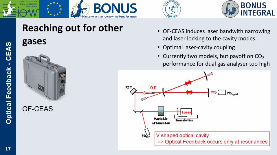
OF-CEAS

• OF-CEAS induces laser bandwith narrowing and laser locking to the cavity modes

• Optimal laser-cavity coupling• Currently two models, but payoff on CO2

performance for dual gas analyser too high

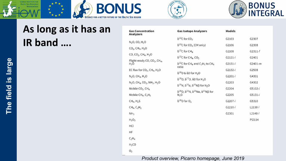
As long as it has anIR band ….

Product overview, Picarro homepage, June 2019

The

field

isla

rge

Is there a “best technology”?

19

Bes

t ins

trum

ent?

Maybe not• ICOS ATC, after intensive testing, accepts (only)

Picarro G2301 (CO2, CH4, H2O) and G2401 (CO, CO2, CH4, and H2O) for CO2 and CH4

• But only LGR N2OCM-913 for N2O• In principle, oa-ICOS should have advantages in

terms of vibration issues and „do it yourself“ needs.

• Oa-ICOS has largest inner volume, though• New players on the market (like Miro Analytics,

an EMPA (Switzerland) offspring with supportfrom ETH Zürich

• Ocean community might have other qualitycriteria

Peak broadening and matrix effects

20

Peak

bro

aden

ing

Asorption Peak Shape controls

• Minimum Peak widths given by Heisenberg uncertainty principle (neglible)

• Movement of gas molecules leads tosymmetric Doppler broadening (Gauss shaped)

• Pressure or collisional broadening occursowing to collisions between the particles, which disturb the emission and absorptionprocess, depending on pressure, cross section, and velocity (Lorenz shaped)

• Pathlength between collisions short comparedto wavelength => Peak narrowing

• Resulting profile is called Galatry Profile (Galatry, 1963)

• Most instruments measure the peak heigth, which is depending on peak broadening

Δ" Δ# = ℎ2'

Ocean surface applications

Difficultiesforoceanapplications

• Change of bulk gas composition– Changes in O2/Ar/N2 ratio– MATRIX effect

• Larger dynamic range than atmosphericcommunity

– Choice of instrument– Issues with calibration gases

Becker et al. 2012;-0.3 ppm CO2 for a 380ppm gas at 2% oxygenoversaturation

Trace Gas System for RV-based operations• 3 laser-based detection

systems• Los Gatos GGA (CH4 and CO2)

• Los Gatos N2O/CO Analyser

• Picarro 2131 (CO2, d13CCO2)

• High flow through equilibration system

• Parallel setup of internal sensor pumps

• Additional short circuit air pump

• High water flow-through (8.5 L/min)

• Coupled bubble-type shower head type

reactor

• High exchange in resulting foam level

CEA

S ap

plic

atio

non

RVs

PeltierCooler

CRDS d13CCO2 Oa-ICOS CO2/CH4

Oa-ICOS CO/N2O

N2

CG

CEA

S ap

plic

atio

non

RVs

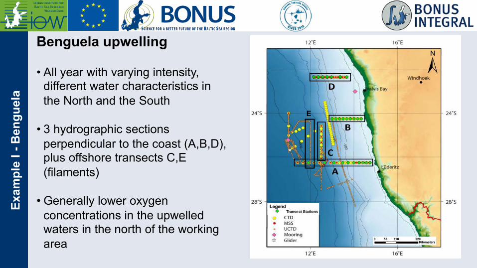
Benguela upwelling

• All year with varying intensity, different water characteristics in the North and the South

• 3 hydrographic sectionsperpendicular to the coast (A,B,D), plus offshore transects C,E (filaments)

• Generally lower oxygenconcentrations in the upwelledwaters in the north of the workingarea

E

Exam

ple

I -B

engu

ela

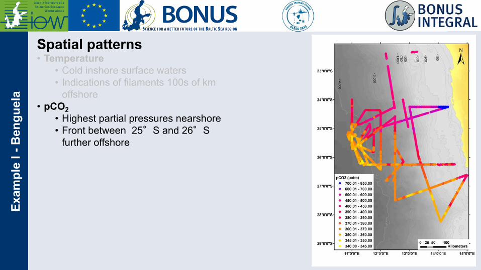
Spatial patterns• Temperature

• Cold inshore surface waters• Indications of filaments 100s of km

offshore

4

Potential temperature (top) and westward velocity (bottom) sections along the Namibian upwelling front as measured during cruise M99 in August 2013 (uncalibrated data). Red dots on top of the upper figure mark the location of UCTD profiles; numbers are UCTD profile numbers. ADCP data were averaged to 10 min ensembles. Acknowledgements We like to thank Captain Klaus Bergmann, his officers and the crew of RV Meteor for their support of our measurement programme, and their hospitality, in particular towards the participating students. The ship time of RV Meteor was provided by the Deutsche Forschungsgemeinschaft within the core program METEOR/MERIAN. Financial support for the project was provided though the German Ministry of Education and Research (SACUS-SPACES). We also benefited from financial contributions by the research institutes involved.

24�S 28�S

Pot. temperature and westward velocity on a UCTD transect between 24�S and 28�S

Exam

ple

I -B

engu

ela



offshore• pCO2

• Highest partial pressures nearshore• Front between 25�S and 26�S

further offshore

Exam

ple

I -B

engu

ela



offshore• pCO2

• Highest partial pressures nearshore• Front between 25�S and 26�S

further offshore• Nitrous oxide

• Comparable patterns to pCO2• Moderate oversaturation of 100 %

Exam

ple

I -B

engu

ela



offshore• pCO2

• Highest partial pressures nearshore• Front between 25�S and 26�S further

offshore• Nitrous oxide

• Comparable patterns to pCO2• Moderate max. oversaturation of 100 %

• Methane• Moderate max. oversaturation of 200 %• High concentrations bound to inshore

upwelled waters

Exam

ple

I -B

engu

ela

North vs. SouthThe effect of the source of upwelled waters

A

B

F

Exam

ple

I -B

engu

ela

VOS

App

licat

ion

-Fin

nmai

d

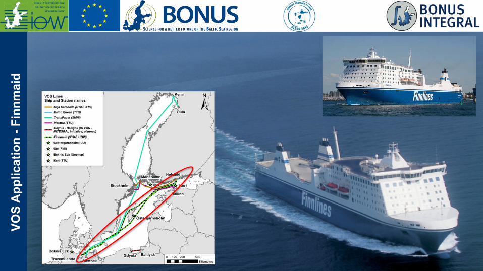
The BALTIC VOS Ferrybox SystemFinnlinesM/S Finnmaid

• Greenhouse gas measurements: pCO2 (twice) and CH4

• Installed alongside pre-existing Finnish Alg@linesystem (Real time algal monitoring in the Baltic Sea)

Description: Gülzow et al., 2011

t: 226 s for CO2, 676 s for CH4

Overview (Methane)• Continuous measurement of CH4 using oa-ICOS on the VOS

Finnmaid• Unique spatiotemporal coverage• Main drivers: SST, mixed layer thickness, upwelling, thermocline

stability

Extended data set from Gülzow et al., 2013

23

!

!

Fig. 20. Methane concentrations (dots) and hydrographic parameters at a station in the central Bornholm Basin in De-cember 2009 (left), and August 2010 (right, with high resolution sampling of the lower 5m). Note jump in methane scale. Bottom waters were characterized by inflow of oxygenated waters at the bottom in December and anoxic conditions in summer, in conjunction with an increase of dissolved methane concentrations from 20 to 80 nM over this period of time.

!

!

Fig. 21. Schematic of a system for the contin-uous measurement of CH4 and pCO2 in sur-face waters using off-axis ICOS. The system is installed on the ferry Finnmaid run by Finn-lines.

!

AB: full basin mixinginducing escape fromsediments

GB: small ASE fluxes except forupwelling events

GoF: mixed layerdeepening andseasonal icecoverage

A gl

imps

e on

the

data

54

56

58

60

12 16 20 24 28Lon °E

Lat °

N

55

56

57

58

59

60

2010 2011 2012 2013 2014 2015 2016 2017Year

Lat °

N

2.5 3 3.5 4 4.5 5 6 7 8 10 12

cCH4 [nmol/L]

Reliability

34

CONSIDERATIONS OF THE RESPONSETIME OF EQUILIBRATION SYSTEMS

A: GENERAL

Webb et al. 2016• Systematic evaluation of

equilibrator response times

• 21�C, 1L/min gas flow, • CH4 response time always larger

than CO2 response time• Ratio smallest for membrane-type

equilibrators

RESP

ONS

ETI

MES

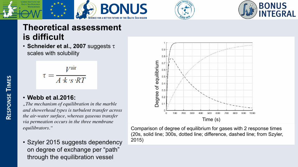
Theoretical assessment is difficult• Schneider et al., 2007 suggests t

scales with solubility

• Webb et al.2016:„The mechanism of equilibration in the marbleand showerhead types is turbulent transfer acrossthe air-water surface, whereas gaseous transfervia permeation occurs in the three membraneequilibrators.“

• Szyler 2015 suggests dependency on degree of exchange per “path” through the equilibration vessel

Deg

ree

ofeq

uilib

rium

Time (s)

Comparison of degree of equilibrium for gases with 2 response times(20s, solid line; 300s, dotted line; difference, dashed line; from Szyler, 2015)

RESP

ONS

ETIMES

37

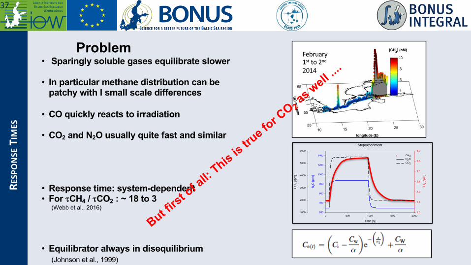
Problem• Sparingly soluble gases equilibrate slower

• In particular methane distribution can be patchy with l small scale differences

• CO quickly reacts to irradiation

• CO2 and N2O usually quite fast and similar

• Response time: system-dependent• For tCH4 / tCO2 : ~ 18 to 3

(Webb et al., 2016)

• Equilibrator always in disequilibrium(Johnson et al., 1999)

February 1st to 2nd

2014

Stepexperiment

Time [s]

0 500 1000 1500 2000

CH

4 [pp

m]

1,0

1,5

2,0

2,5

3,0

3,5

4,0

N2O

[ppb

]

200

400

600

800

1000

1200

1400

CO

2 [pp

m]

1000

2000

3000

4000

5000

6000

CH4N2OCO2

But first of all:

This istru

e for CO2as well ....

RESP

ONS

ETIMES

38W

HAT

ISM

EANT

BY2 µ A

TMAC

CURA

CY

So what is a correct value?

•Implications for“Quality Goals”,i.e. SOCAT, ICOS

Longitude (�E)

39

CONSIDERATIONS OF THE RESPONSETIME OF EQUILIBRATION SYSTEMS

B: DOING THE MATH ...

40TIMELA

GCO

RREC

TION

•Equilibrator always in disequilibrium

(Johnson et al., 1999)

•Bears potential to derive the “true” water value, assuming t is well known and deconvolution scheme is established

41

Correction for equilibration time

corrected methane concentration at

time t+1

Equations introduced in Johnson et al., 1999.Derived following Miloshevich, 2004.

observed apparent methane concentrations

for time t+1 and preceding measurement at time t

time interval between consecutive measurements at times t and t+1, small enough

that the methane concentration can be assumed to be approximately constant

gas and equilibrator (and T and S?) dependent

equilibrator time constant

TIM

ELA

GCO

RREC

TIO

N

42

TIME LAG CORRECTION ON REALDATA

TRACKING THE EFFECT OF UPWELLING

43

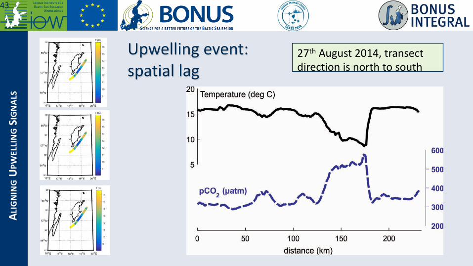
Upwelling event: spatial lag

27th August 2014, transect direction is north to south

ALIGNING

UPWELLING

SIGNA

LS

44

44

ALIGNING

UPWELLING

SIGNA

LS

45AL

IGNING

UPWELLING

SIGNA

LS

46

Upwelling event: spatial lag- Effect on relation to SST

ALIGNING

UPWELLING

SIGNA

LS

47


T decreasing (entering upwelling), CH4increasing.

ALIGNING

UPWELLING

SIGNA

LS

48



T increasing (leaving upwelling), no corresponding decrease in CH4

Rehder et al.: Continuous measurement of CH4 and pCO2 in the Baltic Sea using oa-ICOS on a VOSAL

IGNING

UPWELLING

SIGNA

LS

49



T increasing (leaving upwelling), no corresponding decrease in CH4

T steady (no longer in upwelling region), CH4decreasing with time lag

Rehder et al.: Continuous measurement of CH4 and pCO2 in the Baltic Sea using oa-ICOS on a VOSAL

IGNING

UPWELLING

SIGNA

LS

50


Correction with tCH4= 540 s

ALIGNING

UPWELLING

SIGNA

LS

51

Correction with tCH4= 540 s


ALIGNING

UPWELLING

SIGNA

LS

Response Time• VGas minimization not an option• Reduction of gas in equilibration

chamber reduces fraction of residence of gas in the active exchanging part

• Enhancement of k only option => get bigger

11

3.1 Stufenexperiment

Für das Stufenexperiment wurden zwei ca. 900 l fassende Wasserbassins mit Wasser

unterschiedlicher Methankonzentration gefüllt. Eine Wassertonne wurde mit normalen

Leitungswasser gefüllt, die andere Tone wurde mit zuvor Methanübersättigten Wasser versetzt.

Hierzu wurde 1 l Wasser in einer Schottflasche 5 Minuten mit 100% Methan begast. Aus der Flasche

wurden genau 40 ml entnommen und in die Wassertonne gegeben, welche anschließend mit

Leitungswasser auf 700 l aufgefüllt wurde. Um einen Austausch der beiden Wasserbassins mit der

Umgebungsluft zu verhindern, wurden Styroporplatten mit gasdichter Folie ummantelt und als

schwimmender Deckel auf die beiden Wasseroberflächen gegeben. Mit einer Druckwasserpumpe

wurde das Wasser zum Equilibrator gepumpt. Die Pumpe ließ sich über einen Druckminderer in ihren

Durchflussgeschwindigkeiten regeln. Als erstes wurde das Wasser aus der Tonne mit dem normalen

Leitungswasser zum Equilibrator gepumpt. Wenn sich ein konstanter Methangehalt eingestellt hat,

wurde mittels Dreiwegeventil zur zweiten Tonne umgeschaltet, welche ebenfalls bis zur Einstellung

eines konstanten Wertes gepumpt worden ist. Dann wurde erneut zum normalen Leitungswasser

umgeschaltet um so die Abklingkurve zu erhalten.

Abbildung 7: Beispiel eines Stufenexperiments bei einem Durchfluss von 9 l/min und einem zusätzlichen Gasdurchfluss von 4 l/min.

Im Moment des Wechsels der beiden Wasserbassins beginnt der Methangehalt in der Gasphase sich

dem Gleichgewichtspartialdruck des jeweils anderen Wasserbassinsgehalts anzunähern. Er bewegt

sich von der Konzentration p1 zum Zeitpunkt t0 mit der Geschwindigkeit pt zu p2 zum Zeitpunkt t1

bzw. von p2 zurück auf p1. Die Geschwindigkeit hängt vom Grad des Ungleichgewichts und der

Effizienz des Gasaustausches ab.

0,00000

5,00000

10,00000

15,00000

20,00000

25,00000

0 1000 2000 3000 4000 5000

[CH4

] in

ppm

Zeit in s

Stufenexperiment Flow 9 l/min

[CH4] ppm

[CH4] ppm

[CH4] ppm

p1 bei t=t0

p2 bei t=t1

p1 at t=t0

p2 at t=t1

Time (s)

14

Abbildung 10: Zeitkonstanten für Methan der verschiedenen Stufenexperimente

Man erkennt in Abbildung 10 ganz deutlich den Trend, dass mit zunehmender

Wasserdurchflussmenge sich das Gleichgewicht zwischen Wasser und Gasphase schneller einstellt.

Dies scheint jedoch kein linearer Trend zu sein sondern durch andere Faktoren eher limitiert.

Auffällig ist hier, dass ein zusätzlicher Gasstrom bei geringer Durchflussmenge mehr Einfluss auf die

Zeitkonstante nimmt als bei hoher. Ebenso erstaunlich ist, dass der geringere zusätzliche

Gasdurchfluss bei hohen Wasserdurchflussmengen mehr Gewicht hat als der, mit der höheren

zusätzlichen Gasdurchflussmenge.

Dass der Einfluss des zusätzlichen Gasdurchflusses bei hohen Wasserdurchflussmengen nicht mehr

den gravierenden Einfluss nimmt, lässt sich durch Beobachtung des Experiments erklären. Bei dem

Wasserflow von nahezu 11 l·min-1 bildeten sich auf der Wasseroberfläche im Equilibrator

Turbulenzen. Das Wasser schäumte beinahe. So hat man natürlich den Headspace automatisch

verkleinert und zusätzlich eine relativ große Austauschfläche geschaffen.

0

100

200

300

400

500

600

700

800

900

1000

3 5 7 9 11

τin

s

Durchfluss l/min

Vergleich τ CH4

250 ml/min Gasdurchsatz

4,7l l/min Gasdurchsatz

2,5l l/min Gasdurchsatz

Water flow (L/min)

Optimized (lab, aboard):t < 30 s (CO2)t < 230 s (CH4)

FASTER

EQUILIBR

ATIONBY

HARD

WAR

E

Take home messages– Surface equilibration technique is straightforward, but a few known

issues are usually neglected (response time, total pressure bias)– New sensors allow for measurement of a large variety of gases, e.g.

nitrous oxide and methane– Deconvolution schemes for time lag so far not usally used, and maybe

not needed in most cases– Response time, which can be assessed upon switch from calibration

mode to surface water measurement, should be part of metadata wherever possible

– CEAS measurement requires standard gases in natural air balance– Matrix effects complicate measurements, in particular addressing stable

isotope ratios

Take

aw

ays

Next generation instrumentation

55

- Instrumentation after ICOS funding– 3 laser-based detection systems– Los Gatos GGA (CH4 and CO2)– Los Gatos N2O/CO Analyser– Picarro 2131 (CO2, d13CCO2)– Spectrophotometric pH (BONUS PINBAL)

– Double oxygen optode

- High flow through system– Parallel setup of internal sensors – Additional short circuit air pump– High water flow-through (8.5 L/min)

61

Flow scheme, mainequilibration system withtwo Los Gatos gas sensors; Equilibration system withmain and help equilibrator

62

Flow scheme, secondequilibration set up withmain and helpequilibrator, one Picarrogas analyser, 2 oxygenoptodes and pH-spectrophotometer

Water mass characteristics

• Intermediate water of sectionA (north) distinct

• Intermediate water of sectionA with higher oxygen levels, both vs T and vs Depth

• Obviously coldest waters atsurface in section B

64

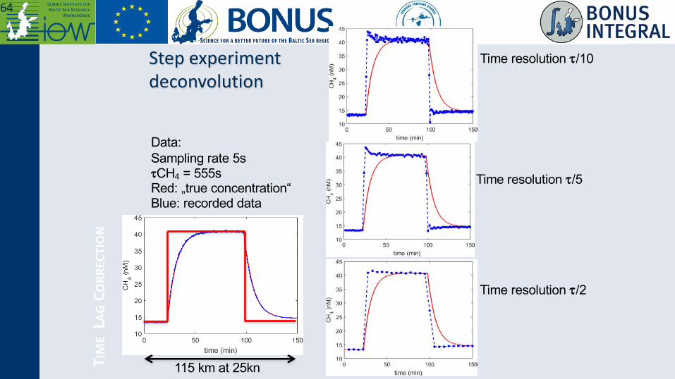
Step experimentdeconvolution

Data:Sampling rate 5stCH4 = 555sRed: „true concentration“Blue: recorded data

Time resolution t/5

Time resolution t/2

Time resolution t/10

115 km at 25knTIMELA

GCO

RREC

TION

65

The following notes briefly outline the calculations used to convert ring down times into absorption intensity. This is done automatically in Picarro CRDS analyzers and is included here only for completeness.The light signal at the photodetector is given byI(t, λ) = I0 e-t/τ( λ)

Where I0 is the transmitted light intensity at the time the laser is switched off and τ(λ) is the ring down time constant. For a given wavelength, λ, the decay rate,R (λ) = 1/τ(λ)is proportional to the optical losses inside the cavity and equal to the empty-cavity decay rate plus a factor dependent on the sample absorption:R (λ,C) = 1/(λ) = R (λ,O) + cε(λ)Cwhere R(λ) = 1/τo(λ) is the empty-cavity decay rate. The effective path length of the measurement is given byLeff = cτo(λ)where c is the speed of light. For typical mirrors having a reflectivity of 99.995% and scattering losses of less than 0.0005 percent, Leff can be over 10 km. For a cell length of 25cm, this is a pathlength enhancement factor of over 20,000.The sample absorption can be written as:α(λ) = ε(λ)CWhere ε is the extinction coefficient and C is the concentration. This can be found by taking the difference between the decay rates of an empty cavity (C = 0) and a cavity containing a sample, i.e.:α(λ) = 1/c[R(λ,c) - R(λ,0)]If the absorption cross section and lineshape parameters of the sample are known, then the concentration of the sample can be readily computed. For a more detailed mathematical treatment of cavity ring down spectroscopy, see K.W. Busch and M.A. Busch (1997). "Cavity ring-down spectroscopy: An ultratrace absorption measurement technique." ACS Symposium Series 720, Oxford.

BTW:The Network Status

European Network within Ocean Branch of ICOS

SOCONET

66

Introduciton

This scheme of comparing the ring down time of the cavity without anyabsorbing gas, with the ring down time when a target gas is absorbing light isaccomplished not by removing the gas from the cavity, but rather by using a laser whose wavelength can be tuned. By tuning the laser to different wavelengths where the gas absorbs light, and then to wavelengths where thegas does not absorb light, the "cavity only" ring down time can be compared tothe ring down time when a target gas is contributing to the optical loss withinthe cavity. In fact, the laser is tuned to several locations across the targetgas's spectral absorption line (and ring down measurements are conducted at all these points) and a mathematical fit to the shape of that absorption line iswhat is actually used to calculate the gas concentration.

At Picarro we solved this problem by developing and patenting our ownwavelength monitor. It can measure absolute laser wavelength to a precision more than 1000 times narrower than the observed Doppler-broadened linewidth for small gas phase molecules. We then use this in a novel way - specifically, we lock the laser to the wavemeter, which wethen actively tune to known wavelengths. The result is higher spectralprecision than in any commercial spectrometer - laser-based orotherwise. This spectral precision is the key to the ultra-precise fitting oflineshapes and line heights necessary to reach parts per trillionconcentration sensitivity.

CEAS • Measures Absorption from the mirror-transmitted intensity

68

ND

IR a

ndG

O

oa-ICOS :This approach deliverssuperior performance, yet is orders-of-magnitude less sensitive to internal alignment of components and tovariations in local temperature andpressure

In addition, variations in the concentrations of a gas with a permanent dipole (like CO2 or H2O) can even cause subtlechanges in the shape of a non-overlapped line, forexample CH4 — a well-known effect called pressurebroadening.

Cavity Ring Down Spectroscopy • Cw pumping until threshold

• Patented wavelength monitor measureabsolute laser wavelength to a precisionmore than 1000 times narrower than theobserved Doppler-broadened linewidth forsmall gas phase molecules.

• Laser locked to the wavemeter, which wethen actively tune to known wavelength.

69

CRDS

Documents

Session 12: Equilibrator-based surface measurements