Embed Size (px)
Citation preview
Economic Research Service
Economic Research Report Number 174
September 2014
United States Department of Agriculture
Global Drivers of Agricultural Demand and Supply
Ronald D. Sands, Carol A. Jones, and Elizabeth Marshall
Economic Research Service www.ers.usda.gov
The U.S. Department of Agriculture (USDA) prohibits discrimination in all its programs and activities on the basis of race, color, national origin, age, disability, and, where applicable, sex, marital status, familial status, parental status, religion, sexual orientation, genetic information, political beliefs, reprisal, or because all or a part of an individual’s income is derived from any public assistance program. (Not all prohibited bases apply to all programs.) Persons with disabilities who require alternative means for communication of program information (Braille, large print, audiotape, etc.) should contact USDA’s TARGET Center at (202) 720-2600 (voice and TDD).
To file a complaint of discrimination write to USDA, Director, Office of Civil Rights, 1400 Independence Avenue, S.W., Washington, D.C. 20250-9410 or call (800) 795-3272 (voice) or (202) 720-6382 (TDD). USDA is an equal opportunity provider and employer.
United States Department of Agriculture
Access this report online:
www.ers.usda.gov/publications/err-economic-research-report/err174
Download the charts contained in this report:
• Go to the report’s index page www.ers.usda.gov/publications/ err-economic-research-report/err174
• Click on the bulleted item “Download err174.zip”
• Open the chart you want, then save it to your computer
Recommended citation format for this publication:
Sands, Ronald D., Carol A. Jones, and Elizabeth Marshall. Global Drivers of Agricultural Demand and Supply, ERR-174, U.S. Department of Agriculture, Economic Research Service, September 2014.
Cover image: istock.
Use of commercial and trade names does not imply approval or constitute endorsement by USDA.
United States Department of Agriculture
Economic Research Service
Economic Research Report Number 174 September 2014
Abstract
Recent volatility in agricultural commodity prices and projections of world population growth raise concerns about the ability of global agricultural production to meet future demand. This report explores the potential for future agricultural production to 2050, using a model-based analysis that incorporates the key drivers of agricultural production, along with the responses of producers and consumers to changes to those drivers. Model results show that for a percentage change in population, global production and consumption of major field crops respond at nearly the same rate. In response to a change in per capita income, the per-centage change in crop consumption is much lower, about one-third the percentage change in income. The model also suggests that the global economy absorbs changes in agricultural productivity growth through compensating responses in yield, cropland area, crop prices, and international trade.
Keywords
Agricultural productivity, food demand, population growth, income growth, land use
Acknowledgments
The authors thank Cheryl Christensen, Scott Malcolm, and Paul Westcott of USDA’s Economic Research Service (ERS); Ruben Lubowski of the Environmental Defense Fund’s International Climate Program; and Dominique van der Mensbrugghe of Purdue University for their comments and suggestions. We also thank John Weber and Curtia Taylor (USDA-ERS) for editorial and design assistance.
Ronald D. Sands, Carol A. Jones, and Elizabeth Marshall
Global Drivers of Agricultural Demand and Supply

Contents
Summary . . . . . . . . . . . . . . . . . . . . . . . . . . . . . . . . . . . . . . . . . . . . . . . . . . . . . . . . . . . . . . . . . . . . . iii
Introduction . . . . . . . . . . . . . . . . . . . . . . . . . . . . . . . . . . . . . . . . . . . . . . . . . . . . . . . . . . . . . . . . . . . .1
Economic Framework and Study Design . . . . . . . . . . . . . . . . . . . . . . . . . . . . . . . . . . . . . . . . . . . .3
Data Overview . . . . . . . . . . . . . . . . . . . . . . . . . . . . . . . . . . . . . . . . . . . . . . . . . . . . . . . . . . . . . . . . . .6
Agriculture to 2050: A Reference Scenario . . . . . . . . . . . . . . . . . . . . . . . . . . . . . . . . . . . . . . . . .10
Population . . . . . . . . . . . . . . . . . . . . . . . . . . . . . . . . . . . . . . . . . . . . . . . . . . . . . . . . . . . . . . . . . . . .15
Income and Food Consumption Per Person . . . . . . . . . . . . . . . . . . . . . . . . . . . . . . . . . . . . . . . . .18
Agricultural Productivity . . . . . . . . . . . . . . . . . . . . . . . . . . . . . . . . . . . . . . . . . . . . . . . . . . . . . . . .22
Historical Growth in Agricultural Production: Decomposition of Source . . . . . . . . . . . . . . . . . .26
Analysis Across Drivers . . . . . . . . . . . . . . . . . . . . . . . . . . . . . . . . . . . . . . . . . . . . . . . . . . . . . . . . .28
Summary and Future Direction . . . . . . . . . . . . . . . . . . . . . . . . . . . . . . . . . . . . . . . . . . . . . . . . . .30
References . . . . . . . . . . . . . . . . . . . . . . . . . . . . . . . . . . . . . . . . . . . . . . . . . . . . . . . . . . . . . . . . . . . .31
Appendix A . FARM Documentation . . . . . . . . . . . . . . . . . . . . . . . . . . . . . . . . . . . . . . . . . . . . . . .36
Introduction . . . . . . . . . . . . . . . . . . . . . . . . . . . . . . . . . . . . . . . . . . . . . . . . . . . . . . . . . . . . . . . . .36
Production Activities . . . . . . . . . . . . . . . . . . . . . . . . . . . . . . . . . . . . . . . . . . . . . . . . . . . . . . . . . .37
CGE Framework . . . . . . . . . . . . . . . . . . . . . . . . . . . . . . . . . . . . . . . . . . . . . . . . . . . . . . . . . . . . .39
Demand . . . . . . . . . . . . . . . . . . . . . . . . . . . . . . . . . . . . . . . . . . . . . . . . . . . . . . . . . . . . . . . . . . . .39
Supply . . . . . . . . . . . . . . . . . . . . . . . . . . . . . . . . . . . . . . . . . . . . . . . . . . . . . . . . . . . . . . . . . . . . . .40
Substitution Elasticities in FARM . . . . . . . . . . . . . . . . . . . . . . . . . . . . . . . . . . . . . . . . . . . . . . . .45
Income and Own-Price Elasticities of Demand in FARM . . . . . . . . . . . . . . . . . . . . . . . . . . . . . .46
Appendix B . Decomposition Methodology . . . . . . . . . . . . . . . . . . . . . . . . . . . . . . . . . . . . . . . . . .50

United States Department of Agriculture
A report summary from the Economic Research Service
ERS is a primary source of economic research and
analysis from the U.S. Department of Agriculture, providing timely informa-
tion on economic and policy issues related to agriculture, food, the environment, and
rural America. www.ers.usda.gov
Find the full report at www.ers.usda.
gov/publications/err-economic-research-
report/err174
Economic Research Service
Economic Research Report Number 174
September 2014
United States Department of Agriculture
Global Drivers of Agricultural Demand and Supply
Ronald D. Sands, Carol A. Jones, and Elizabeth Marshall
Ronald D. Sands, Carol A. Jones, and Elizabeth Marshall
Global Drivers of Agricultural Demand and Supply
What Is the Issue?
Recent volatility in agricultural commodity prices, coupled with projections of world popula-tion growth, raise concerns about the ability of global agricultural production to meet future demand. A number of factors are likely to affect the potential for future agricultural production. These include demand drivers such as changes in population and per capita income, as well as supply drivers such as changes in agricultural productivity. The world’s population is projected to grow from 7 billion to approximately 9 billion by 2050, and per capita income is projected to grow in nearly all the world’s regions. Agricultural productivity has improved rapidly in recent decades, but prospects for future growth are uncertain, especially in light of climate change. ERS examines hypothetical economic and agricultural effects of potential changes in agricultur-al productivity, population, and per capita income by 2050. These supply-and-demand drivers will determine not only what farmers will produce in the future, where they will produce it, and how affordable it will be, but also how much land and other scarce resources the sector will use.
What Did the Study Find?
• Effects of a change in population. For a 10-percent increase in global population, total crop consumption and production is projected to respond at nearly the same rate. Crop yield, however, increases by only 5 percent for this increase in population, even as increased demand for agricultural commodities pushes prices higher and encourages producers to use more yield-enhancing inputs. Crop area also responds to higher crop prices in this popula-tion scenario, with an expected increase in area of 4 percent.
• Effects of a change in per capita income. For a 10-percent increase in global per capita income, consumption and production of major crops is projected to increase by approxi-mately 3 percent. Crop yield increases by 3 percent in this scenario, and cropland area increases by less than 1 percent.
• Effects of a change in agricultural productivity. A negative shock to global agricultural productivity could come about through a decrease in investments in agricultural research and development over time or through other economic or environmental factors such as climate change. This study did not simulate climate change, but it did consider a 20-percent decline in global productivity by 2050 for major field crops. The primary adjustments to the
September 2014

www.ers.usda.gov
change in productivity are in crop yield and cropland area. Through increased use of nonland inputs such as fertilizer and capital equipment, the realized decline in crop yield of 12 percent is less than the initial decline in productivity. To further compensate for the effects of the shock, land area supplied for field crops is projected to increase by 14 percent. At a global level, crop consumption and production are equal, and both decline slightly. World trade volume increases as crop production shifts among world regions. Average prices for field crops increase by 15 percent in this scenario, providing incentives to expand land area and increase use of nonland inputs in agricultural production.
For all scenarios, the percentage change in crop production is approximately the sum of percentage changes in yield and cropland area.
How Was the Study Conducted?
This study was conducted in parallel with a global economic analysis of potential climate impacts organized by the Agricultural Model Intercomparison and Improvement Project (AgMIP). The Future Agricultural Resources Model (FARM) used in this study is 1 of 10 participating models that incorporate global coverage of major field crops and other crop types. FARM is an economic model that simulates agricultural and energy systems for 13 world regions through 2050. Primary data sources include the United Nations (population projections), the Food and Agriculture Organization of the United Nations (agricultural production), the International Energy Agency (energy balances), and the Global Trade Analysis Project at Purdue University (social accounts).
A global reference scenario through year 2050 was constructed using medium-fertility population projec-tions, moderate income growth, and crop productivity data (assuming no climate change impacts) provided by AgMIP to each modeling team. Model output includes consumption and production of agricultural com-modities, yield and world prices of major field crops, and land use by crop type. To isolate the sensitivity of model variables to key drivers, a number of additional scenarios were constructed that varied the values of individual drivers one at a time, relative to the reference scenario: low- and high-population scenarios; a low-income scenario; and two low-productivity scenarios.
An elasticity is the ratio of percent changes: the percent change in an economic response (e.g., consumption) for each percent change in a driver (e.g., income). When population or income is the driver, economic responses move in the same direction. Yield moves in the same direction as productivity, while cropland area and price move in the opposite direction of productivity. YIELD = average yield of major field crops in tons per hectare. AREA = global area of major field crops. CONS = global consumption = global production. TRADE = global exports = global imports. PRICE = price index of major field crops: wheat, rice, coarse grains, oil seeds, and sugar.Source: USDA, Economic Research Service using Future Agricultural Resources Model scenarios.
Elasticities of economic responses to three key drivers
Elasticity
Population Income Productivity
-0.8
-0.6
-0.4
-0.2
0.0
0.2
0.4
0.6
0.8
1.0
1.2
YIELD AREA CONS TRADE PRICE

1 Global Drivers of Agricultural Demand and Supply, ERR-174
Economic Research Service/USDA
Introduction
Recent volatility in prices of agricultural commodities and projections of world population growth raise concerns about the ability of global agricultural production to meet future demand. The world’s population is projected to grow by approximately 2 billion by 2050. Per capita incomes are project-ed to grow in nearly all world regions over the same period. Agricultural productivity has improved rapidly in past decades, but prospects for future growth are uncertain, especially in light of climate change. How would the change in population affect the demand for major field crops? How would the increase in per capita incomes affect per capita consumption of crops? How would the global economy absorb a negative shock to agricultural productivity? How sensitive are crop prices to projected changes in population, income, and agricultural productivity?
To help answer these questions, this study uses the Future Agricultural Resources Model (FARM) to simulate agricultural demand, supply, and land use for 13 world regions from 2005 through 2050 (see box “The Future Agricultural Resources Model”). First, researchers construct a global reference scenario through year 2050 using projections on population growth, income growth, and agricultural productivity. This reference scenario represents one potential snapshot of the future, based on a set of moderate but uncertain projections of population, income, and agricultural productivity growth rates. The reference scenario then provides a point of departure for analyses exploring the respon-siveness of model outputs to changes in these key drivers of supply and demand varied one at a time. Within each world region, land is allocated to crops, pasture, or forest based on economic returns per hectare of land (1 hectare = 2.47 acres). In each scenario, demand for agricultural products is driven primarily by population and income. Prices of field crops and processed agricultural products adjust to bring agricultural markets into equilibrium.
Ronald D. Sands, Carol A. Jones, and Elizabeth Marshall
Global Drivers of Agricultural Demand and Supply

2 Global Drivers of Agricultural Demand and Supply, ERR-174
Economic Research Service/USDA
The Future Agricultural Resources Model
The Future Agricultural Resources Model (FARM) is a global economic model with 13 world regions and operates from 2004 to 2054 in 5-year steps. Model output is usually interpolated to report results in more convenient years, such as 2030 or 2050. Land use can shift among crops, pasture, and forests in response to population growth, changes in agricultural productivity, and environmental policies, such as efforts to mitigate climate change.
The first version of FARM was constructed in the early 1990s by Roy Darwin and others at USDA’s Economic Research Service (Darwin et al., 1995). Early versions of the model were used to simulate the impact of a changed climate on global land use, agricultural production, and international trade. Recent versions of FARM add a time dimension to assess alternative climate policies, track energy consumption and greenhouse gas emissions, and provide a balanced repre-sentation of world energy and agricultural systems. FARM model development has benefited from participation in the Agricultural Model Intercomparison and Improvement Project (AgMIP) and the Stanford Energy Modeling Forum (EMF). Research in this report uses consensus scenarios from the AgMIP project.
The FARM base year is 2004, which is the base year of a global economic data set distributed by the Global Trade Analysis Project (GTAP) at Purdue University. ERS uses social accounts in GTAP version 7 as the primary economic framework. GTAP 7 provides social accounting matrices for 112 world regions and 57 production sectors. These data are then aggregated to 13 world regions and 38 production sectors for this study. The 38 production sectors retain all GTAP information related to primary agriculture, food processing, energy transformation, energy-inten-sive industries, and transportation. Participation in AgMIP requires substantial expansion of the agricultural component of FARM.
One of the most important features of FARM is the land-allocation mechanism. For each world region, land competition takes place within agro-ecological zones (AEZs) that differ by growing period and climatic zone. Land is allocated to crops, pasture, and managed forest through a land market in each AEZ.

3 Global Drivers of Agricultural Demand and Supply, ERR-174
Economic Research Service/USDA
Economic Framework and Study Design
Table 1 provides a summary of supply-and-demand drivers examined in this study.
Two other important drivers are not covered in this report, but results using the FARM model are published elsewhere:
• Climate and energy policy (demand side). Examples of the policy dimension include green-house gas cap-and-trade and renewable portfolio standards (Sands et al., 2014a; Sands et al., 2014b). Bioenergy links the energy and agricultural systems, increasing demand for crop-land or forest land.
• Climate change (supply side). Agricultural productivity changes over time, due to changing temperature, precipitation, and humidity. Climate impacts vary by world region and crop type. The AgMIP global economic study provides simulations to 2050 driven by several climate and crop process models (Nelson et al., 2014a; Nelson et al., 2014b).
Population over the model time horizon is entered directly into FARM as an exogenous input.1 Income growth is entered indirectly, by adjusting labor productivity in each world region to ap-proximate income projections from another source.2 Each production sector in FARM has a set of productivity parameters that can be set directly as annual rates of productivity change. Economic impacts of climate change can also be modeled as changes in productivity parameters for crops, informed by projections from climate models and crop growth models.
FARM includes markets for agricultural products and land to calculate key outputs (see table 2). Because of interactions between markets, most of these output variables are calculated simultane-ously.3
1An exogenous model input or parameter is determined outside the model, and the model has no influence over this input or parameter.
2 It is common for general equilibrium models to use labor productivity as a parameter to align the path of Gross Domestic Product (GDP) with projections derived from other sources. In FARM, we adjust labor productivity for all production sectors at the same rate within each world region. Here, we align GDP for each world region in FARM with projections from the Shared Socioeconomic Pathways (O’Neill et al., 2014).
3 See appendix A for more information on FARM.
Table 1
Summary of drivers of agricultural supply and demand in this report
Population(demand side)
Low, medium, and high population projections through 2050.
Income(demand side)
Income growth that contributes to increasing per capita consumption of food over time. Shift in diet toward processed foods and meat.
Agricultural productivity(supply side)
The technology dimension as a driver of agricultural production and land use, allowing crop yields to vary, holding agricultural resource use constant.
4 Global Drivers of Agricultural Demand and Supply, ERR-174
Economic Research Service/USDA
The effect of an increase in population is to increase demand, which raises prices. Producers will respond to higher prices by increasing production, using some combination of increasing cropland and increasing inputs per unit of land. Individual consumers respond to higher prices by shifting consumption to less expensive food types, and, possibly, reducing consumption. Global shifts in trade reflect patterns of consumption that diverge from patterns of production.
Model results depend on model structure and selection of behavioral parameters, such as price and income elasticities of demand; the tradeoff among inputs to agricultural production; and the ability of land to be transformed between various crops, pasture, and forest (see table 3).4
The world reference scenario simulated through 2050 for this analysis accounts for projections of population, per capita income, and agricultural productivity. Population projections are from the United Nations medium-fertility scenario (United Nations, 2011). Income projections by world region are from socioeconomic scenarios recently prepared for modeling the impacts of climate change by the international modeling community (O’Neill et al., 2014). In the reference scenario, per capita income grows rapidly in regions such as China, India, and Sub-Saharan Africa. Changes in land productivity through 2050 are provided by the International Food Policy Research Institute (IFPRI).
To determine the responsiveness of model outputs to changes in population, income, and growth in agricultural productivity, inputs are varied one at a time (see table 4). Shaded cells in the table repre-sent deviations from the reference scenario.
World population in the reference scenario grows from nearly 7 billion people in 2004 to approxi-mately 9 billion people in 2050. The low-income scenario represents a 29-percent decline in world average per capita income from the reference scenario in 2050. The reference scenario provides a view of drivers of supply and demand changing over time. Given the uncertainty of these drivers, other scenarios examine alternative specifications and variations in results across scenarios in 2050.
4 An elasticity is the percentage change in one variable in response to the percentage change in another variable or parameter. For example, the income elasticity of demand is the percentage change in a consumed product in response to a percentage change in income.
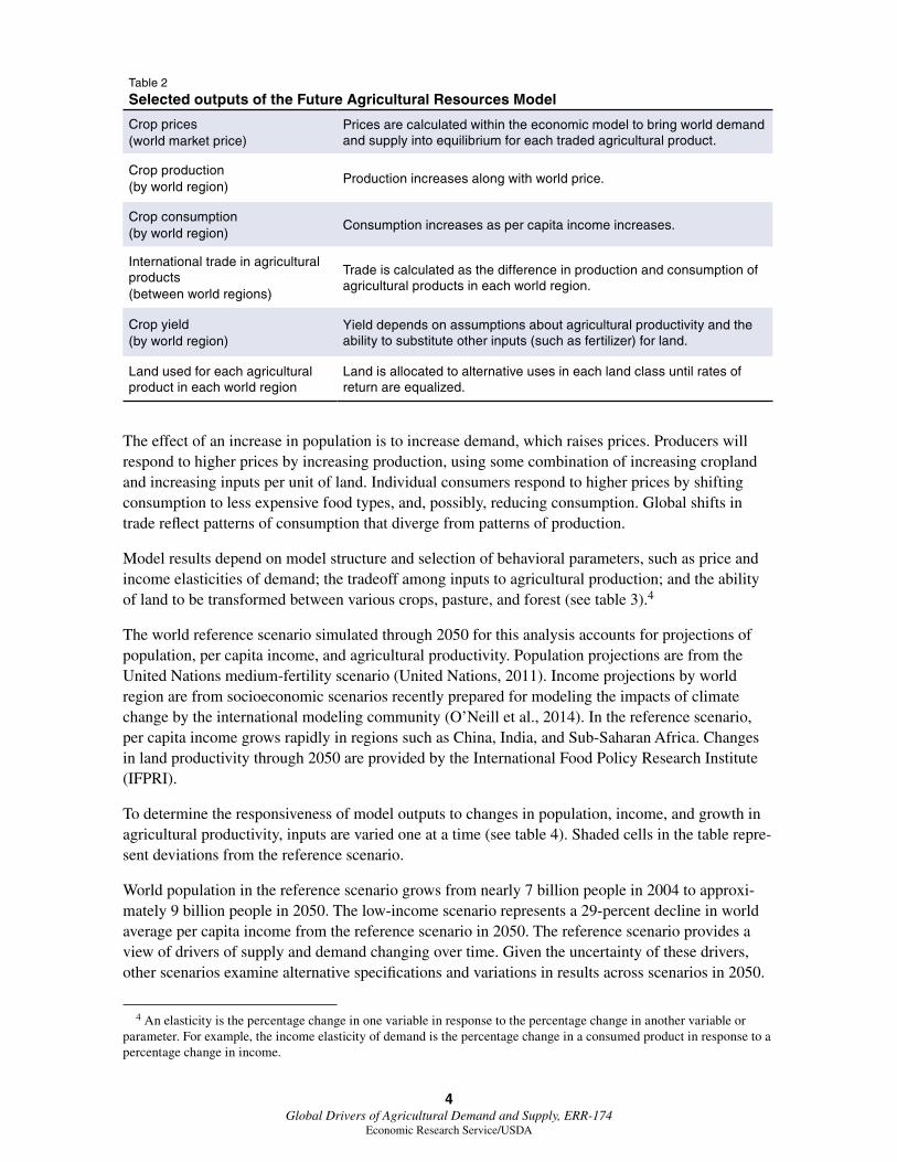
Table 2
Selected outputs of the Future Agricultural Resources Model
Crop prices(world market price)
Prices are calculated within the economic model to bring world demand and supply into equilibrium for each traded agricultural product.
Crop production(by world region)
Production increases along with world price.
Crop consumption(by world region)
Consumption increases as per capita income increases.
International trade in agricultural products(between world regions)
Trade is calculated as the difference in production and consumption of agricultural products in each world region.
Crop yield(by world region)
Yield depends on assumptions about agricultural productivity and the ability to substitute other inputs (such as fertilizer) for land.
Land used for each agricultural product in each world region
Land is allocated to alternative uses in each land class until rates of return are equalized.

5 Global Drivers of Agricultural Demand and Supply, ERR-174
Economic Research Service/USDA
Table 3
Behavioral parameters in the Future Agricultural Resources Model
Price elasticity of demand for agricultural products
Rate at which food consumption declines as price increases.
Income elasticity of demand for agricultural products
Rate at which food consumption increases as income increases.
Elasticity of substitution among inputs to production
Tradeoffs among inputs to production such as capital, labor, land, fertilizer, and energy.
Table 4
Overview of scenarios designed to capture economic responses to changes in key drivers: population, per capita income, and agricultural productivity
Chapter Scenario Population Income Productivity
Agriculture to 2050: A Reference Scenario
Reference UN-medium Reference growth Optimistic
Population Low population UN-low Reference growth Optimistic
Population High population UN-high Reference growth Optimistic
Income and Food Conumption Per Person
Low income UN-medium Low growth Optimistic
Agricultural Productivity
Low productivity UN-medium Reference growth20-percent
reduction by 2050
Agricultural Productivity
Very low productivity
UN-medium Reference growth40-percent
reduction by 2050
Note: Scenarios are designed to modify one driver at a time, indicated by the shaded cells. UN=United Nations.

6 Global Drivers of Agricultural Demand and Supply, ERR-174
Economic Research Service/USDA
Data Overview
Data for the FARM model base year are primarily from the GTAP version 7 data set. This includes input-output tables and other social accounts measured in U.S. dollars, as well as data on crop pro-duction (metric tons) and land use (hectares). These data were aggregated from 112 world regions in the GTAP 7 database to 13 world regions (see table 5).
Figure 1 provides a snapshot of production and consumption across 13 FARM regions for 5 major field crops in the base year, 2004. Production for each field crop is measured in tons, and the aggre-gate measure is the sum across these five crop types. Production and consumption are equal at the global level but vary across regions. Canada, the United States, Brazil, Australia, and New Zealand are net exporters of field crops; India is mostly self-sufficient with little net trade; and the largest importing regions are Middle East and North Africa, and Southeast and East Asia.
The world’s 13 billion hectares of land cannot be easily partitioned into categories such as agriculture, forest, pasture, and other uses. For example, some forested land is also used for grazing. Figure 2 provides an overall picture of global land use in seven land-use categories provided by GTAP. India is unique for having a high share of total land as cropland. Built-up land is a small share of total land use across all regions.5
5 Land-use definitions vary across sources, especially for forest land. See the Food and Agriculture Organization (FAO) of the United Nations (2010) for alternative estimates of world forest land. Nickerson et al. (2011) provide a more detailed set of land-use types for the United States. Total cropland compares reasonably well, but some cropland is idle or used for pasture in the United States.
Table 5
Thirteen world regions in FARM
Symbol Description
CAN Canada
USA United States
BRA Brazil
OSA South and Central America countries other than Brazil
FSU Former Soviet Union
EUR Europe (excluding Turkey)
MEN Middle East and North Africa (including Turkey)
SSA Sub-Saharan Africa
CHN China
IND India
SEA Southeast and East Asia countries other than China
OAS South Asian countries other than India
ANZ Australia, New Zealand, and Oceania
FARM = Future Agricultural Resources Model.

7 Global Drivers of Agricultural Demand and Supply, ERR-174
Economic Research Service/USDA
Figure 1
Production and consumption of five major field crops in 2004
Million metric tons
0
100
200
300
400
500
600
CAN USA BRA OSA FSU EUR MEN SSA CHN IND SEA OAS ANZ
Production Consumption
Note: See table 5 for abbreviations of region names. The five crop types are rice, wheat, coarse grains, oil seeds, and sugar. Measures of aggregate production and consumption are the total weight in tons across these five crop types.
Source: USDA, Economic Research Service using the GTAP 7 database.
Note: See table 5 for abbreviations of region names. Source: USDA, Economic Research Service using the GTAP 7 database.
Figure 2
Benchmark land use by world region in 2004
Billion hectares
0
0.5
1.0
1.5
2.0
2.5
CAN USA BRA OSA FSU EUR MEN SSA CHN IND SEA OAS ANZ
World Region
Built-up land
Other land
Shrub land
Forest
Grassland
Pasture
Cropland

8 Global Drivers of Agricultural Demand and Supply, ERR-174
Economic Research Service/USDA
Global land area is also reported in GTAP by land class and land-use type (see fig. 3).6 FARM uses six land classes that partition land by length of growing period (LGP). Across all land classes, total area for global cropland is approximately 1.5 billion hectares. Land Class 1 is the largest in area but contains the smallest amount of cropland. All land classes have a significant amount of cropland, but Land Classes 3 and 4 contain the most. There is no clear pattern relating crop yield to land class, as this varies by crop, level of irrigation, and world region. Within each FARM region and model time step, land from each land class is allocated to individual crops and other land uses.
The agricultural component of FARM allocates land across crops, pasture, and forest. Crops are partitioned into eight crops or crop types. The five major field crops include wheat, coarse grains, rice, oil seeds, and sugar. The three other crop types are fruits and vegetables, plant-based fibers, and other crops. Other agricultural activities in FARM are meat and dairy production, forestry, and fisheries.
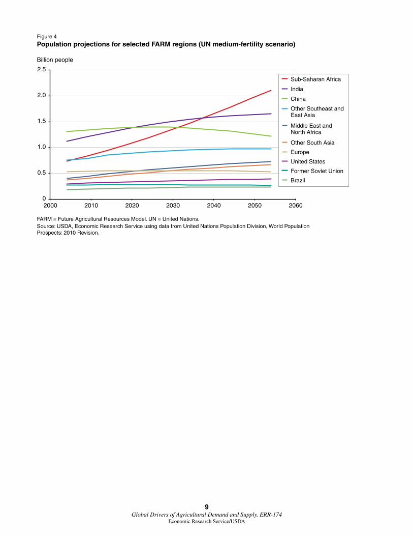
Overall projections of world population through 2050 mask a variety of growth patterns among indi-vidual countries (see fig. 4). India is projected to surpass China as the most populous country around 2020, but Sub-Saharan Africa is expected to surpass India by 2040. The populations of India, China, and Brazil are all expected to peak and decline in the 21st century whereas the U.S. population will increase slowly but continuously.
6 Land use in GTAP is partitioned into 18 agro-ecological zones (AEZs). We aggregated GTAP AEZs into six land classes based on length of growing period (LGP), with approximately 60 days separating the midpoint of each land class. Land Class 1 has an LGP of 0 to 59 days, while Land Class 6 has an LGP greater than 300 days. The six land classes divide the world into areas of progressively increasing humidity: arid; dry semi-arid; moist semi-arid; sub-humid; humid; and humid with year-round growing season (Monfreda et al., 2009, p. 42).
Note: Land classes correspond to length of growing period: Land Class 1, 0 to 59 days; Land Class 2, 60 to 119 days; Land Class 3, 120 to 179 days; Land Class 4, 180 to 239 days; Land Class 5, 240 to 299 days; Land Class 6, over 300 days.Source: USDA, Economic Research Service using the GTAP 7 database.
Figure 3
Benchmark global land use by land class in 2004
Billion hectares
Land class
Built-up land
Other land
Shrub land
Forest
Grassland
Pasture
Cropland
0
0.5
1.0
1.5
2.0
2.5
3.0
3.5
4.0
4.5
1 2 3 4 5 6
9 Global Drivers of Agricultural Demand and Supply, ERR-174
Economic Research Service/USDA
FARM = Future Agricultural Resources Model. UN = United Nations.Source: USDA, Economic Research Service using data from United Nations Population Division, World Population Prospects: 2010 Revision.
Figure 4
Population projections for selected FARM regions (UN medium-fertility scenario)
Billion people
0
0.5
1.0
1.5
2.0
2.5
2000 2010 2020 2030 2040 2050 2060
United States
Brazil
Former Soviet Union
Europe
Middle East and North Africa
Sub-Saharan Africa
China
India
Other Southeast and East Asia
Other South Asia

10 Global Drivers of Agricultural Demand and Supply, ERR-174
Economic Research Service/USDA
Agriculture to 2050: A Reference Scenario
The global reference scenario provides a point of comparison for analysis. First, however, it is im-portant to understand the way agricultural productivity changes over time in the reference scenario. This begins with an exogenous productivity index for each of eight crop types that increase over time (see fig. 5a). This index is considered to be land augmenting: less land is needed per unit of product, but requirements for other inputs per unit of product are not affected.7 Average annual per-centage growth rates range from 0.93 to 1.88 percent across crop groups, between 2005 and 2030.8 Growth rates decline across all crop groups from 2030 to 2050.
If the ratio of each input to unit of product were fixed in each year, then figure 5a would show the yield of each crop type. However, the ratios of all inputs to unit of product respond to prices to achieve equilibrium between demand and supply for each crop type. In particular, equilibrium yield will increase if crop prices increase relative to prices of inputs such as fertilizer, land, labor, and capital equipment.
7 Exogenous productivity drivers in figure 5a are from the IMPACT model maintained by the International Food Policy Research Institute. IMPACT values are based on expert opinion about potential biological yield gains for crops in individual countries and on historical yield gains and expectations about future private and public sector research and extension efforts. These estimates do not include crop model-based climate change effects or economic model yield responses to changes in input or output prices (Nelson et al., 2014a).
8 Annual percentage growth rates based on figure 5a are lower than historical growth rates of world cereal yield, which averaged 2.0 percent per year from 1961 through 2009 (Fuglie, 2012).
Note: These productivity indexes are ratios of productivity in 2050 or 2030 to productivity in 2005 (they are not annual percentage growth rates).Source: USDA, Economic Research Service using data from International Food Policy Research Institute.
Figure 5a
Land-augmenting agricultural productivity index (2005 = 1)
Reference scenario model input (exogenous drivers)
0.0
0.5
1.0
1.5
2.0
2.5
Wheat Rice Oilseeds
Coarsegrains
Sugarcrops
Othercrops
Fruitsand
vegetables
Plant-based fibers
2005 2030 2050

11 Global Drivers of Agricultural Demand and Supply, ERR-174
Economic Research Service/USDA
Global average yield by crop type in the FARM reference scenario increases in all eight crop groups over time (fig. 5b). Average annual percentage growth rates range from 0.84 to 2.18 percent across crop groups, between 2005 and 2030. Most of the increase is due to assumptions about land-aug-menting crop productivity (see fig. 5a), but some of the increase is price induced.
Prices in FARM adjust so that world markets clear for all crops (fig. 6).9 Price increases are modest, due to the large increases in land-augmenting agricultural productivity. In general, if yield in figure 5b is greater than the corresponding land-augmenting productivity index in figure 5a, crop prices increase over time (fig. 6).
For each agricultural commodity, demand equals supply at the global level. Trade allows for differ-ences in demand and supply at the regional level:
exports + (population × per-capita consumption) = (harvested area × yield) + imports
Figure 7a shows the increase in world demand for five major crops across 45 years in the FARM reference scenario. The increase in demand for each crop is partitioned into two explanatory factors: population growth and income growth. These changes in crop demand are large: increases range from 68 percent for wheat to 102 percent for sugar, with an average increase of 77 percent for the five crop types added together. Of this 77-percent increase, 50 percent is attributed to population growth and the remaining 27 percent to increasing incomes.
9 Prices are adjusted for inflation.
Note: These yield indexes are ratios of crop yield in 2050 or 2030 to crop yield in 2005 (they are not annual percentage growth rates). Source: USDA, Economic Research Service using Future Agricultural Resources Model reference scenario.
Figure 5b
World average yield index of major crop groups (2005 = 1)
Reference scenario model output (combining exogenous and endogenous effects)
0.0
0.5
1.0
1.5
2.0
2.5
Wheat Rice Oilseeds
Coarsegrains
Sugarcrops
Othercrops
Fruitsand
vegetables
Plant-based fibers
2005 2030 2050

12 Global Drivers of Agricultural Demand and Supply, ERR-174
Economic Research Service/USDA
Figure 6
World average prices for major crops, reference scenario
Sources: USDA, Economic Research Service using GTAP 7 database; Future Agricultural Resources Model reference scenario.
Constant U.S. dollars per metric ton
0
50
100
150
200
250
300
2000 2010 2020 2030 2040 2050
Sugar
Oil seeds
RiceWheat
Coarse grains
Figure 7a
Components of change in world crop demand (2004-49), reference scenario
Note: Numbers in parentheses are 2004 world production levels in million metric tons.Sources: USDA, Economic Research Service using GTAP 7 database; Future Agricultural Resources Model reference scenario.
Million metric tons
0
100
200
300
400
500
600
700
800
Wheat(632)
Coarse grains(1039)
Rice(608)
Oil seeds(559)
Sugar(146)
Population-induced response
Income-induced response

13 Global Drivers of Agricultural Demand and Supply, ERR-174
Economic Research Service/USDA
Valin et al. (2014) provide a comparison of food demand through 2050 across 10 global economic models in AgMIP, along with a comparison to FAO projections to 2050 (Alexandratos and Bruin-sma, 2012). Food demand in metric tons is reported for ruminant meat, nonruminant meat, dairy products, and crops consumed directly. FAO uses income projections for 2050 that are lower than income projections used by AgMIP models, contributing to projections of food demand that are generally lower than the AgMIP average.
Differences over time in food demand across AgMIP models primarily reflect different functional forms and parameterization of the response of per capita food consumption to rising incomes, espe-cially for developing countries. Projections from the FARM model are near the AgMIP average for consumption of meat and dairy products but above the AgMIP average for crops consumed directly. Figure 7a reports total consumption of crops, including crops used indirectly for meat and dairy products.
Figure 7b provides a decomposition of the supply side into changes in yield and harvested area for select crops.10 At the global level, a change in demand must equal the corresponding change in sup-ply. Prices adjust within FARM to enforce the equality between world supply and demand for each commodity. Most of the increase in world food supply is due to increases in yield. The change in
10 The decomposition method used here is the logarithmic mean Divisia index (LMDI). See Ang (2005) for a guide on using this method to decompose a change in a multiplicative relationship into additive components.
Figure 7b
Components of change in world crop supply (2004-49), reference scenario
Note: Numbers in parentheses are 2004 world production levels in million metric tons.Sources: USDA, Economic Research Service using GTAP 7 database; Future Agricultural Resources Model reference scenario.
Million metric tons
-200
0
200
400
600
800
1,000
Harvested area
Yield
Wheat(632)
Coarse grains(1039)
Rice(608)
Oil seeds(559)
Sugar(146)

14 Global Drivers of Agricultural Demand and Supply, ERR-174
Economic Research Service/USDA
harvested area is relatively small for each crop in this reference scenario.11 The net change in total harvested area is slightly negative.
As shown in figure 8, the main feature of the reference scenario pattern of land use is that total world cropland (five crops plus three crop types) is stable over time, primarily because of optimistic assumptions of agricultural productivity growth (fig. 5a). The total of cropland, pasture, and forest land is constrained to be constant over time.12
In a future that resembles the one constructed under the reference scenario, the increased demand for agricultural products associated with greater incomes and a larger population can be met without significant increases in cropland area or product prices. The increases in agricultural productivity assumed by the reference scenario are sufficient to keep up with growing demand for agricultural products. That future is uncertain, however, and the results are sensitive to the assumptions used to construct the reference scenario.
11 The FARM model base year is 2004 and is solved every 5 years until 2054. Most charts with FARM output are interpolated to show results from 2005 through 2050. However, the LMDI decomposition holds only at model time steps, and here we report the change from 2004 through 2049.
12 We do not simulate expansion of managed land into unmanaged forest. Schmitz et al. (2014) provide a comparison of land use across 10 economic models participating in the AgMIP global economic study. Expansion of cropland is constrained in models with land competition among crops, pasture, and forest, such as FARM.
Figure 8
World agricultural land-use simulation, reference scenario
* The five major field crops are rice, wheat, coarse grains, oil seeds, and sugar. The three other crop types are fruits and vegetables, plant fibers, and other crops. Managed forest is accessible forest land.Sources: USDA, Economic Research Service using GTAP 7 database; Future Agricultural Resources Model reference scenario.
Billion hectares
Major crops*
Other crops*
Managed forest*
Pasture
0
1.0
2.0
3.0
4.0
5.0
6.0
2005 2010 2015 2020 2025 2030 2035 2040 2045 2050
15 Global Drivers of Agricultural Demand and Supply, ERR-174
Economic Research Service/USDA
Population
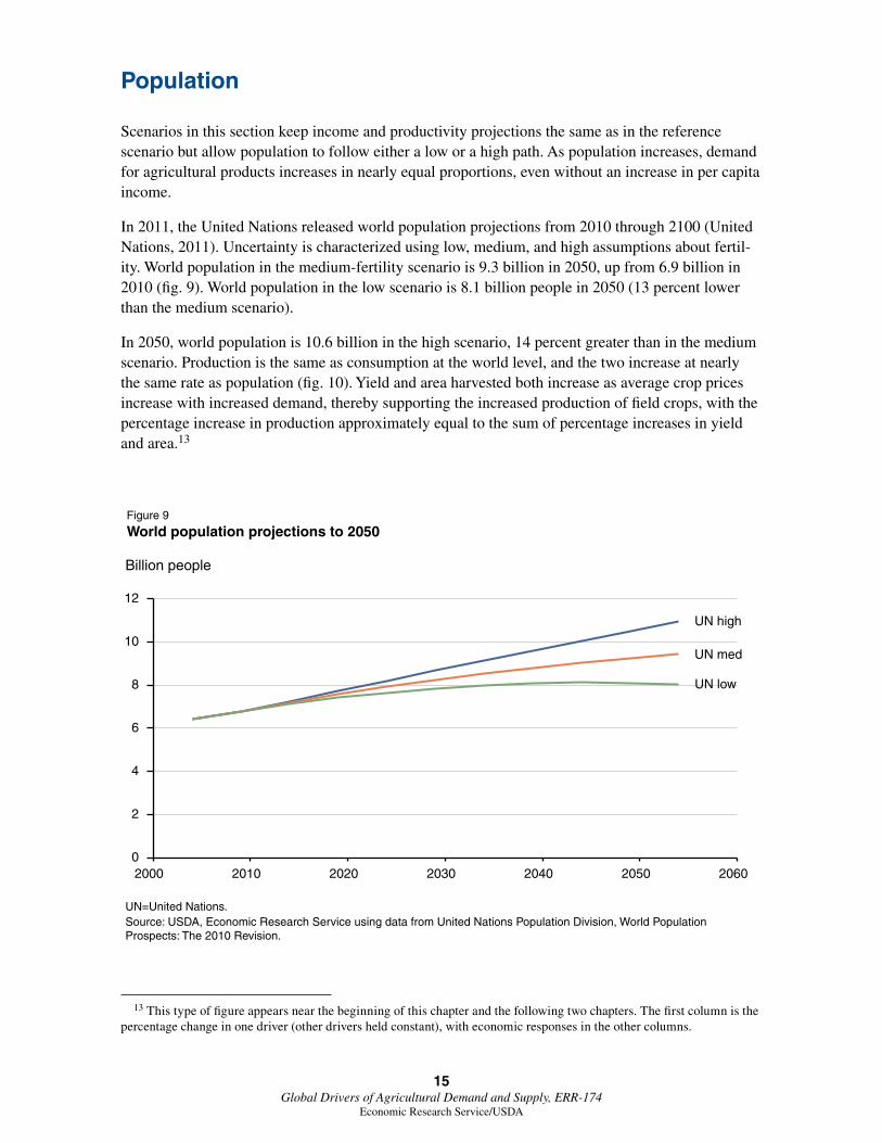
Scenarios in this section keep income and productivity projections the same as in the reference scenario but allow population to follow either a low or a high path. As population increases, demand for agricultural products increases in nearly equal proportions, even without an increase in per capita income.
In 2011, the United Nations released world population projections from 2010 through 2100 (United Nations, 2011). Uncertainty is characterized using low, medium, and high assumptions about fertil-ity. World population in the medium-fertility scenario is 9.3 billion in 2050, up from 6.9 billion in 2010 (fig. 9). World population in the low scenario is 8.1 billion people in 2050 (13 percent lower than the medium scenario).
In 2050, world population is 10.6 billion in the high scenario, 14 percent greater than in the medium scenario. Production is the same as consumption at the world level, and the two increase at nearly the same rate as population (fig. 10). Yield and area harvested both increase as average crop prices increase with increased demand, thereby supporting the increased production of field crops, with the percentage increase in production approximately equal to the sum of percentage increases in yield and area.13
13 This type of figure appears near the beginning of this chapter and the following two chapters. The first column is the percentage change in one driver (other drivers held constant), with economic responses in the other columns.
Figure 9
World population projections to 2050
UN=United Nations.Source: USDA, Economic Research Service using data from United Nations Population Division, World Population Prospects: The 2010 Revision.
Billion people
UN high
UN med
UN low
0
2
4
6
8
10
12
2000 2010 2020 2030 2040 2050 2060

16 Global Drivers of Agricultural Demand and Supply, ERR-174
Economic Research Service/USDA
Figure 11 provides a decomposition of changes in crop demand and supply into changes in two demand components (population and income) and two supply components (yield and harvested area). Data in the figure reflect global supply and demand, with imports equal to exports. If the fig-ure instead included data pertaining to an individual country or world region, the data would reflect changes in exports and imports.
Increasing population drives an increase in crop demand across low-, medium (reference)-, and high-population scenarios, with a combination of yield increase and land-use change on the supply side. Global land-use declines (relative to the reference population growth scenario) in the low-population scenario for five major field crops. Global cropland changes very little in the reference scenario but increases in the high-population scenario.
Figure 10
Economic responses to an increase in world population in 2050High population scenario relative to medium population scenario
Note: Economic responses cover five major field crop types: rice, wheat, coarse grains, oil seeds, and sugar. The driver is world population. YIELD = average yield of major field crops in tons per hectare. AREA = global area of major field crops. CONS = global consumption = global production. TRADE = global exports = global imports. PRICE = price index across the major field crops.Source: USDA, Economic Research Service using Future Agricultural Resources Model scenarios.
Percent
0
2
4
6
8
10
12
14
16
Population YIELD AREA CONS TRADE PRICE

17 Global Drivers of Agricultural Demand and Supply, ERR-174
Economic Research Service/USDA
Figure 11
Components of change in world crop demand and supply, 2004-49
Notes: This figure shows demand and supply for the sum of five major field crops: rice, wheat, coarse grains, oil seeds, and sugar. Changes in demand and supply are the total change over a 45-year horizon. Production levels in 2004 are 3.0 billion metric tons in all scenarios; therefore, production in the high-population scenario is approximately double production in 2004. Components for the reference scenario equal the sum of columns from figures 7a and b. UN = United Nations.Sources: USDA, Economic Research Service using GTAP 7 database; Future Agricultural Resources Model reference scenario.
Population scenarios (billion metric tons relative to 2004 levels)
-0.5
0
0.5
1.0
1.5
2.0
2.5
3.0
Supply(UN low)
Demand(UN low)
Supply(UN high)
Demand(UN high)
Demand(ref)
Supply(ref)
Harvested area
Yield
Population-induced response
Income-induced response

18 Global Drivers of Agricultural Demand and Supply, ERR-174
Economic Research Service/USDA
Income and Food Consumption Per Person
This section presents a scenario with lower income growth over time relative to the reference scenar-io. For example, income growth may be lower if educational attainment and access to public health care is lower than in the reference scenario. By 2050, per capita Gross Domestic Product (GDP) is 29 percent less in the low-growth scenario than in the reference scenario (fig. 12). Per capita GDP still grows over time in the low-growth scenario, just not as fast as in the reference scenario.
In the low-growth scenario, population and crop productivity growth rates are the same as those in the reference scenario, but GDP grows more slowly in all world regions.14 Economic responses to this change are shown in figure 13, with the low-growth scenario relative to the reference scenario.
Lower per capita income growth leads to decreased demand for animal protein, which leads to decreased demand for crops used as animal feed. However, the decrease in consumption of field crops is much smaller, on a percentage basis, than the decrease in per capita income. This pattern of decreased consumption of animal products along with declining per capita income is apparent in historical food consumption across countries of varying per capita income.15 As in figure 10,
14 GDP growth rates are from two of five Shared Socioeconomic Pathways (SSPs): SSP2 for reference growth and SSP3 for low growth. O’Neill et al. (2014) provide an overview of, and motivation for, SSPs. The SSP data are available at https://secure.iiasa.ac.at/web-apps/ene/SspDb. Income pathways from SSP2 and SSP3 are used here for easy compari-son with other model results assessed in the AgMIP global economic modeling study (Nelson et al., 2014a).
15 See box “Food Balance Sheets” for background and historical variation of per capita consumption of animal prod-ucts for India, China, Brazil, and the United States.
Figure 12
Projections of world average real GDP per capita
GDP = Gross Domestic Product.Source: USDA, Economic Research Service projections derived from Shared Socioeconomic Pathways SSP2 and SSP3.
Dollars in 2004
Reference growth
Low growth
0
2,000
4,000
6,000
8,000
10,000
12,000
14,000
16,000
2000 2010 2020 2030 2040 2050 2060

19 Global Drivers of Agricultural Demand and Supply, ERR-174
Economic Research Service/USDA
the percentage change in production is approximately the sum of percentage changes in yield and harvested area.
Box figure 2 displays world average per capita consumption of three food categories over time. Global per capita consumption increased in all three food categories from 1961 through 2007, reflecting world economic growth. It is quite possible for per capita consumption of crops to peak and decline in the future, as consumption patterns in developing countries shift toward patterns in wealthy countries such as the United States.
Figure 13
Economic responses to a decrease in world income in 2050Low-growth scenario relative to reference scenario
Note: Economic responses cover five major field crop types: rice, wheat, coarse grains, oil seeds, and sugar. The driver is per capita income. YIELD = average yield of major field crops in tons per hectare. AREA = global area of major field crops. CONS = global consumption = global production. TRADE = global exports = global imports. PRICE = price index across the major field crops.Source: USDA, Economic Research Service using Future Agricultural Resources Model scenarios.
Percent
-35
-30
-25
-20
-15
-10
-5
0INCOME YIELD AREA CONS TRADE PRICE

20 Global Drivers of Agricultural Demand and Supply, ERR-174
Economic Research Service/USDA
Food Balance Sheets
Food balance sheets describe the total supply and use of various categories of food in a country for a given year. Food balance sheets for groups of countries can be constructed by summing sheets of individual countries for each food category.1 Supply is equal to the quantity of food pro-duced, plus imports, adjusted for any change in stocks. Use includes crops or food consumed by households, used for seed, processed for food and nonfood use, and exports. Except for statistical error, total supply should equal total use.
The Food and Agriculture Organization (FAO) of the United Nations is the primary source of food balance sheets, with detailed coverage of food commodities (FAO, 2001). FAO provides food balance sheets on an annual basis beginning in 1961. FAO food balance sheets group com-modities into cereals, oil crops, starchy roots, sugar crops, pulses, tree nuts, fruits, vegetables, spices, stimulants, sugar and sweeteners, vegetable oils, alcoholic beverages, meats and animal fats, eggs, milk, fish, and seafood. For this study, commodities are combined to match the crops and crop types in the Global Trade Analysis Project (GTAP) database.
The basic unit used in FAO food balance sheets is metric tons per year. The quantity of final con-sumption by households is then converted to kilograms per person per year using that country’s population. Finally, household consumption is converted to units of kilocalories per person per day. This unit enables one to sum calories across commodities and compare diets across countries and over time.
Note that there can be confusion between large calories and small calories, where 1 large calorie equals 1,000 small calories. The calories used in nutrition labels at grocery stores are large calo-ries. FAO food balances use small calories, but they are always displayed as kilocalories (kcal). Therefore, 1 kcal is the same as 1 large calorie familiar to consumers.
Box figure 1 provides a cross-country comparison of food consumption in three broad categories: crops consumed directly, crops consumed indirectly as processed crops, and animal products. The food categories are aggregates of detailed food types in food balance sheets constructed by FAO. Direct crop consumption consists primarily of cereals but also includes starchy roots, food legumes, fruits, and vegetables. Processed crops include vegetable oils from oil crops, sweeten-ers from sugar crops, and alcoholic beverages. Animal products include meat, milk, butter, eggs, and animal fats.
Per capita consumption of total calories varies widely across countries, with the United States well above the world average and India below. The type of calories consumed also varies, for example, with very low per capita consumption of animal products in India relative to other countries with a comparable standard of living. Primary calories include all food or feed crops, while secondary calories include processed crops or animal products. More than one primary calorie is required to produce each calorie of processed crop or animal product, with more primary calories needed for animal products than for processed crops. The implication is that per capita consumption of total primary calories increases along with the quantity of animal products. Residents of wealthier countries generally consume more total calories and more animal products than residents of other countries. Even without population growth, total demand for crops would increase as China and India become wealthier and animal products become a larger share of total calories. However, income-related growth in per capita consumption of
—continued
1 Sums include trade between countries within each grouping of countries.

21 Global Drivers of Agricultural Demand and Supply, ERR-174
Economic Research Service/USDA
Food Balance Sheets—continued
animal products may be less in India than in other countries due to dietary restrictions associated with religious beliefs.
Note: “crops” includes all crops, not just the five major field crop types.Source: USDA, Economic Research Service using data from Food and Agriculture Organization of the United Nations food balance sheets.
Box figure 1
Per capita food consumption in select countries in 2007
kcal per person per day
CropsProcessed cropsAnimal products
0
500
1,000
1,500
2,000
2,500
3,000
3,500
4,000
World average
UnitedStates
Brazil China India
Note: “crops” includes all crops, not just the five major field crop types.Source: USDA, Economic Research Service using data from Food and Agriculture Organization of the United Nations food balance sheets.
Box figure 2
Increasing per capita food consumption over time (world average)
kcal per person per day
Crops
Processed crops
Animal products
0
200
400
600
800
1,000
1,200
1,400
1,600
1,800
1960 1965 1970 1975 1980 1985 1990 1995 2000 2005 2010

22 Global Drivers of Agricultural Demand and Supply, ERR-174
Economic Research Service/USDA
Agricultural Productivity
Scenarios in this section keep population and income the same as in the reference scenario but examine the effects of lower growth in agricultural productivity. These scenarios reflect considerable uncertainty about the future growth in agricultural productivity in the face of global climate change, unpredictable public and private investment decisions concerning agricultural research and develop-ment (R&D), and myriad other factors that could affect productivity trends. Two low-productivity scenarios were constructed: one with a 20-percent decline in land-augmenting productivity relative to the reference scenario by 2050 and another with a 40-percent decline. Agricultural productivity still increases through 2050 in the 20-percent low-productivity scenario, just not as fast as in the ref-erence scenario. When comparing productivity levels in 2050, the low-productivity scenarios appear as a negative productivity shock relative to the reference scenario.
Figure 14 shows how the global economy absorbs the hypothetical decline in productivity growth in 2050. Actual yield does not fall as much as land productivity because other inputs increase as crop prices increase. The productivity shock is largely absorbed both through intensification of agricul-tural production and through an increase in harvested area. Production and consumption decline slightly as consumers adjust spending patterns in response to higher prices of food. Again, as in figures 10 and 13, the percentage change in production is approximately the same as the sum of percentage changes in yield (in this case, negative) and area harvested.
Figure 14
Economic responses to a 20-percent decline in agricultural productivity in 2050*
* The 20-percent decline was selected because it is close to the average productivity decline in Nelson et al. (2014b), a modeling study of potential climate impacts on world agriculture. Note: Responses cover five major crop types: rice, wheat, coarse grains, oil seeds, and sugar. The driver is a change in productivity (PRODUCTIVITY), the change in yield holding nonland inputs to production constant. YIELD = average yield in tons per hectare, allowing increases in nonland inputs to production. AREA = global area of major field crops. CONS = global consumption = global production. TRADE = global exports = global imports. PRICE = price index across the major field crops.Source: USDA, Economic Research Service using Future Agricultural Resources Model scenarios.
Percent
-25
-20
-15
-10
-5
0
5
10
15
20
PRODUCTIVITY YIELD AREA CONS TRADE PRICE

23 Global Drivers of Agricultural Demand and Supply, ERR-174
Economic Research Service/USDA
Earlier in this study, the reference scenario was developed using exogenous drivers for land-aug-menting productivity provided by AgMIP (see fig. 5a). Land use for crops remains stable through 2050 with the reference scenario’s productivity assumptions (see fig. 8), which are lower than historical productivity growth rates. However, more land is used for crops in the low-productivity scenarios. Figure 15 shows the increase in cropland from 2005 through 2050 in the very low pro-ductivity scenario, with a corresponding decrease in pasture and managed forest.16 World cropland grows 28 percent during the period, from 1.40 billion hectares to 1.79 billion hectares.
The most striking difference between the low-productivity and very-low-productivity scenarios is the change in average price for major crops. The price increase is 16 percent in the low-productivity scenario but 99 percent in the very-low-productivity scenario.
The sources of agricultural output growth can be partitioned into increases in land in production and changes in crop yield. Yield growth (output per unit of land) represents—in a single indicator—mul-tiple sources of production growth. One source is farmer intensification of inputs, such as irriga-tion, fertilizer, and capital equipment per unit of land in response to price signals. Another source is increases in total factor productivity (TFP), which reflects improved technologies and improved
16 A 20-percent decline in productivity is approximately the world average decline by 2050 in AgMIP climate impact scenarios (Nelson et al., 2014a; Nelson et al., 2014b). The 40-percent productivity decline scenario was selected as an extreme case.
Figure 15
World agricultural land-use simulation—very-low-productivity scenario (40 percent less than reference scenario)
* The five major field crops are rice, wheat, coarse grains, oil seeds, and sugar. The three other crop types are fruits and vegetables, plant fibers, and other crops. Managed forest is accessible forest land.Sources: USDA, Economic Research Service using GTAP 7 database; Future Agricultural Resources Model scenario.
Billion hectares
Major crops*
Other crops*
Managed forest*
Pasture
0
1.0
2.0
3.0
4.0
5.0
6.0
2005 2010 2015 2020 2025 2030 2035 2040 2045 2050
24 Global Drivers of Agricultural Demand and Supply, ERR-174
Economic Research Service/USDA
management resulting from long-term R&D investments. 17 Agricultural productivity has improved rapidly in past decades, but prospects for future growth are uncertain, especially in the context of climate change (see box “Climate Change as an Emerging Driver”).
Growth in agricultural output relative to total agricultural land area (total yield) has paralleled the trends in output growth, remaining fairly steady at an average of about 2.1 percent per year from 1961 through 2007. Increases in yield are attributed to a combination of new high-yielding, fertiliz-er-responsive seed varieties, in conjunction with major increases in fertilizer use and the expansion of irrigation or better water control within irrigated systems (Heisey and Norton, 2007). However, the relative contributions of input intensification and TFP growth have reversed over time, as the annual growth in TFP rose from 0.2 percent in the 1960s to about 1.7 percent since 1990, and the growth in inputs per unit of land fell commensurately.
17 Productivity can be characterized using measures of total-factor productivity (TFP) or partial-factor productivity (PFP). TFP is an index that measures output per unit of all inputs and measures the extent to which fewer resources are required to produce a given level of output. As such, TFP can be interpreted as a signal of technical change or improved efficiency in the use of inputs. An alternative productivity index, partial-factor productivity (PFP), measures output per unit of a particular input. For example, yield growth (output per unit of land) is a partial productivity measure. However, both TFP and PFP are imperfect measures of innovation because they also reflect economies of scale, as well as changes over time in key environmental conditions affecting yields: local growing conditions (length of growing season and pre-cipitation), soil quality, and the availability of water for irrigation.
Climate Change as an Emerging Driver
Land-use change has traditionally been explored from the perspective of changing economic and social conditions within a constant biophysical regime. In recent decades, however, concerns regarding fundamental changes in climate systems have resulted in increased attention to the relationship between climate change and land use.1
A large body of research has explored land-use change as a contributing factor in climate change by inventorying the carbon sequestration capacity of different land uses and estimating how movement of land from forest to agriculture, for instance, changes terrestrial carbon storage capacity and atmospheric carbon concentration. An exploration of how crop production and land use might respond to climate change, however, has been constrained by limited availability of robust future climate projections and uncertainty about how such climate projections translate into the more short-term regional weather patterns that strongly influence how land-use decisions are made. The emergence of an ensemble of climate projections from both the fourth and fifth Assessment Reports of the Intergovernmental Panel on Climate Change (IPCC) has loosened that limitation somewhat. Based on a common set of emissions scenarios, all of the IPCC climate projections estimate an increase in global mean surface air temperature, with the largest temperature increases over land and at northern latitudes (IPCC, 2007 and 2013). While there is considerable variability among the projections in the details of regional
—continued
1 The role of climate change in global economic models of agriculture is the current topic of study in the Agricul-tural Model Inter-comparability and Improvement Project (AgMIP). Background on AgMIP can be found at www.agmip.org

25 Global Drivers of Agricultural Demand and Supply, ERR-174
Economic Research Service/USDA
Climate Change as an Emerging Driver—continued
precipitation, they generally project increased precipitation in tropical areas that experience large precipitation events, such as monsoon regions, over the tropical Pacific, and at high latitudes. Precipitation is generally projected to decrease in subtropical dry regions, with dry midlatitude regions projected to get drier, and wet midlatitude regions likely to get wetter by the end of the century (IPCC, 2013).
Globally variable changes in temperature, precipitation, length of growing season, and incidence of extreme weather events will have region- and crop-specific impacts on agricultural productiv-ity and yields. The IPCC (2007) broadly projects positive yield impacts for 1-3º C temperature change within temperate regions, but several studies of climate change impacts within the United States have projected mixed impacts of climate change on crop yields in the short term (Reilly et al., 2003; McCarl, 2008; Beach et al., 2010; Malcolm et al., 2012). The results of such studies are highly sensitive to whether and how the yield-enhancing effects of atmospheric carbon dioxide are considered in the analysis (Reilly et al., 2007; Cline, 2007).
Even in the short term, however, climate change is expected to have a much more negative impact on agricultural yields in developing countries (Parry et al., 2004; Fischer et al., 2005; Hertel et al., 2010). Productivity may be more negatively affected because many developing countries are already at the upper end of their temperature ranges, and precipitation is not expected to increase as it is in many temperate regions (Easterling et al., 2007; Mertz et al., 2009). Evidence suggests climate change has already slowed the growth in crop yields over recent decades in India (e.g., Auffhammer et al., 2006) and globally (Lobell et al., 2011). Regardless of short-term effects, many researchers project that as continuing temperature increases exceed critical thresholds in the mid-to-late century, crop yields will eventually decline both within the United States and worldwide (Parry et al., 2004; Schlenker et al., 2005; Schlenker and Roberts, 2009; IPCC, 2007; Burke et al., 2011). Though such studies often focus on the direct yield impacts of climate condi-tions on crop growth, agricultural productivity will be further affected by climate change impacts on ecosystem services that agriculture relies on, such as pollination, pest pressures, water sup-plies, and flood control.
Altered growing conditions are likely to have significant impacts on patterns of relative productiv-ity of managed systems in the provision of food, feed, fiber, and fuel products worldwide. Such significant changes in economic opportunity often lead to land-use change, as decisionmakers adjust their land-use decisions to take advantage of new opportunities or to minimize the effects of new constraints (Lambin et al., 2001). Climate adaptation—or the human response to the changing constraints and opportunities associated with climate change—has been identified as a potentially significant driver of future patterns of land use worldwide, particularly with respect to changes in agricultural land use. Changing patterns of land use as an adaptation strategy will be constrained by the regional availability of land suited for agriculture. The estimated impacts of climate change on the global availability of suitable land for agriculture are mixed and sensitive to the climate scenarios used (Zhang and Cai, 2011). In general, however, studies estimate that arable land increases at the higher latitudes, including Canada, Russia, Northern United States, and Southern Argentina, and decreases in Western Africa, Central America, Western Asia, the South-Central United States, and Northern South America (Ramankutty et al., 2002; Zhang and Cai, 2011).

26 Global Drivers of Agricultural Demand and Supply, ERR-174
Economic Research Service/USDA
The pattern in yield growth has varied across commodities. For example, the cereal yield growth rate has shown signs of slowing after 1990: global cereal yield increased by about 2.5 percent per year in the 1970s and 1980s but by only 1.3 percent per year during 1991-2009 (Fuglie, 2012). However, the pattern for cereals does not appear to be representative of agriculture as a whole. It has been offset by productivity improvements elsewhere—rising yield growth in other commodities and greater intensification of land use—to keep total output per hectare of agricultural land rising at historical rates.
Historical Growth in Agricultural Production: Decomposition of Source
Global agricultural production has increased more than 150 percent over the past five decades (Fug-lie, 2012). The rate of output growth has remained remarkably consistent over the past 50 years—averaging 2.7 percent per year in the 1960s and between 2.1 and 2.5 percent per year every decade since (fig. 16). Over this period, the high rate of growth in production levels occurred primarily through yield growth rather than cropland expansion. However, the sources of yield growth have shifted from intensification of inputs per unit of land to growth in TFP.
From 1961 through 2009, the world’s cultivated area grew by 12 percent. At the same time, global irrigated area doubled, accounting for most of the net increase in cultivated land (fig. 17). Most of the area expansion occurred by 1990. However, the conversion of lands from rainfed to irrigated has continued throughout the period, such that agriculture uses 70 percent of water withdrawn from aquifers, streams, and lakes (FAO, 2011).
TFP = Total factor productivity.Source: USDA, Economic Research Service using data from Fuglie (2012), p. 350.
Figure 16
Sources of global agricultural growth
Percent per year
TFP
TFP
TFPTFP
TFP
TFP
0.5
1.0
1.5
2.0
2.5
3.0
1961-70 1971-80 1981-90 1991-2000 2001-09
TFPInputs/Land
Irrigation
Area expansion
0.01961-2009

27 Global Drivers of Agricultural Demand and Supply, ERR-174
Economic Research Service/USDA
Sources: USDA, Economic Research Service using data from the Food and Agriculture Organization of the United Nations (2011, 2014).
Figure 17
Evolution of world cropland under irrigated and rainfed croppings
Billion hectares
0
0.2
0.4
0.6
0.8
1.0
1.2
1.4
1.6
1.8
1961 1965 1970 1975 1980 1985 1990 1995 2000 2005 2010
Rainfed Area equipped for irrigation

28 Global Drivers of Agricultural Demand and Supply, ERR-174
Economic Research Service/USDA
Analysis Across Drivers
In this study, the sensitivity of model output is observed for changes in reference scenario assump-tions on population, income, and agricultural productivity. Figures 10, 13, and 14 depict the re-sponse of model output variables to changes in each of these drivers. These changes are presented in table 6 for easy comparison. These results were obtained by varying each driver one at a time, holding the other drivers constant.
With population as a driver, the percentage increases in crop consumption (13.5 percent), produc-tion (13.5 percent), and trade volume (14.2 percent) scale at nearly the same percentage rate as population (13.8 percent). This increase in global production is obtained with increases in yield (7.1 percent) and area (5.9 percent). With income as a driver, the percentage change in all economic responses is smaller than the percentage change in income (-29.2 percent). In particular, crop con-sumption falls at a smaller percentage rate (-9.1 percent) than income. With a decline in agricultural productivity, intensification of agricultural production limits the decline in yield (12.4 percent) to be significantly less than the decline in productivity (20.0 percent). However, to keep the decline in global crop production small, harvested area increases (13.8 percent).18
Percentage changes from table 6 can be converted to elasticities: the percentage change in an eco-nomic response divided by the percentage change in one of the drivers. For example, the elasticity of global crop consumption (13.5 percent) with respect to world population (13.8 percent) is 0.98, or nearly one-to-one. Figure 18 presents elasticities of five economic responses with respect to three drivers, allowing a direct comparison across drivers for each economic response. While the scenari-os in these estimates are based on often-modelled declines relative to the reference scenario, elas-ticities are presented as responses to an increase in each driver for easy comparison. For example, the figure shows how an increase in productivity would affect economic indicators: yield increases, harvested area declines, and average price falls.
18 For small changes in harvested area, the percentage change in production is approximately equal to the percent-age change in yield plus the percentage change in area. For larger changes in harvested area, cropland expands into less productive land and the approximation is less accurate.
Table 6
Economic responses to changes in agricultural drivers
Percent change from reference scenario DRIVER YIELD AREA CONS TRADE PRICE
Percent
+13.8 POPULATION 7.1 5.9 13.5 14.2 11.6
-29.2 INCOME -8.1 -1.1 -9.1 -8.9 -0.7
-20.0 PRODUCTIVITY -12.4 13.8 -0.3 5.3 15.3
YIELD = average yield of major field crops in tons per hectare. AREA = global area of major field crops. CONS = global consumption = global production. TRADE = global exports = global imports. PRICE = price index of major field crops: rice, wheat, coarse grains, oil seeds, and sugar.
Source: USDA, Economic Research Service using Future Agricultural Resources Model scenarios.

29 Global Drivers of Agricultural Demand and Supply, ERR-174
Economic Research Service/USDA
The elasticities of crop yield with respect to all three drivers is less than one, with similar responses from population and productivity and less of a response from income. Harvested area responds positively to population and negatively to productivity increases. If both population and productivity increase at the same time, as is assumed in the reference scenario, the combined effects on area may cancel. Global crop consumption, production, and world trade volume respond in a nearly one-to-one ratio with population but with a much smaller response to income. Crop prices move in the same direction as population, but in the opposite direction of productivity. As with area, if popula-tion and productivity increase at the same time, their effects on price may offset each other.
An elasticity is the ratio of percent changes: the percent change in an economic response (e.g., consumption) for each percent change in a driver (e.g., income). When population or income is the driver, economic responses move in the same direction. Yield moves in the same direction as productivity, while cropland area and price move in the opposite direction of productivity. YIELD = average yield of major field crops in tons per hectare. AREA = global area of major field crops. CONS = global consumption = global production. TRADE = global exports = global imports. PRICE = price index of major field crops: wheat, rice, coarse grains, oil seeds, and sugar.Source: USDA, Economic Research Service using Future Agricultural Resources Model scenarios.
Figure 18
Elasticities of economic responses to three key drivers
Elasticity
Population Income Productivity
-0.8
-0.6
-0.4
-0.2
0.0
0.2
0.4
0.6
0.8
1.0
1.2
YIELD AREA CONS TRADE PRICE

30 Global Drivers of Agricultural Demand and Supply, ERR-174
Economic Research Service/USDA
Summary and Future Direction
This study describes economic responses to three drivers of agricultural supply and demand: population, per capita income, and agricultural productivity. Responses to these drivers provide an enhanced understanding of global land use and agricultural markets over time, whether in a con-ceptual model or a formal computational model such as FARM. A conceptual model developed by Hertel (2011) provides qualitative insights on drivers of agricultural demand, supply, and land use in a simple partial-equilibrium framework with a single agricultural product and single region. This study examines numerical relationships between drivers and a set of global economic responses: crop yield, harvested area, consumption, production, trade volume, and average prices.
The analysis started with a reference scenario to 2050 with sufficient gains in agricultural productiv-ity over time to maintain stable cropland area and crop prices. However, productivity growth could be lower depending on the level of future agricultural research or climate change. The reference sce-nario used the medium-fertility population scenario of the United Nations, which includes signifi-cant population growth. If agricultural productivity growth is less than in the reference scenario, or if population growth is greater than in the reference scenario, crop prices increase to provide incen-tives for an increase in cropland area. The increase in cropland area is limited due to competition for land among crops, pasture, and forest.
The reference scenario in this report is the same as contributed by the FARM modeling team to AgMIP. The global economic modeling group of AgMIP recently published a collection of papers in Agricultural Economics that compares results from FARM with nine other global agricultural models and identifies areas for further model improvement. This special issue includes an overview paper (Von Lampe et al., 2014), a methodology paper (Robinson et al., 2014), a food demand paper (Valin et al., 2014), and a land-use paper (Schmitz et al., 2014).
On the demand side, the AgMIP global economic modeling group will continue to examine food demand as it responds to rising per capita income. Each of the global modeling teams adjusted in-come elasticities over time but would prefer an alternative food demand structure that endogenously makes this adjustment in income elasticities. Further analysis is planned for livestock, especially tracking the efficiency of feed-to-meat conversion. Environmental policies that promote biofuels are a relatively recent demand driver for crops and land.
More research is needed on the supply side, especially with respect to agricultural productivity in the context of climate change. Initial analyses using the AgMIP global economic models are pub-lished in Nelson et al. (2014a and 2014b). Other topics that require further attention include integra-tion with process-based crop models, the treatment of water, and extreme events such as a multiyear drought. This study covers global results, but figure 18 shows that international trade can provide an important economic adjustment to supply and demand shocks. This finding suggests that regional analysis may provide interesting response patterns to complement global results.
31 Global Drivers of Agricultural Demand and Supply, ERR-174
Economic Research Service/USDA
References
Alexandratos, N., and J. Bruinsma. 2012. “World Agriculture Towards 2030/2050: the 2012 revi-sion,” ESA Working Paper No. 12-03. Food and Agriculture Organization of the United Nations.
Ang, B.W. 2005. “The LMDI Approach to Decomposition Analysis: A Practical Guide.” Energy Policy 33: 867–871.
Armington, Paul S. 1969. “A Theory of Demand for Products Distinguished by Place of Production,” International Monetary Fund Staff Papers, pp. 159-176.
Auffhammer, Maximilian, V. Ramanathan, and Jeffrey R. Vincent. 2006. “Integrated Model Shows That Atmospheric Brown Clouds and Greenhouse Gases Have Reduced Rice Harvests in India,” Proceedings of the National Academy of Sciences 103: 19668-19672.
Beach, R.H., C. Zhen, A. Thomson, R.M. Rejeseus, P. Sinha, A.W. Lentz, D.V. Vedenov, and B.A. McCarl. 2010. Climate Change Impacts on Crop Insurance. U.S. Department of Agriculture, Risk Management Agency.
Burke, M., J. Dykema, D. Lobell, E. Miguel, and S. Satyanath. 2011. “Incorporating Climate Uncertainty into Estimates of Climate Change Impacts, With Applications to U.S. and African Agriculture,” NBER Working Paper 17092.
Burniax, J.-M., and T.P. Truong. 2002. GTAP-E: An Energy-Environmental Version of the GTAP Model. West Lafayette, IN: Global Trade Analysis Project.
Cline, W.R. 2007. Global Warming and Agriculture: Impact Estimates by Country. Center for Global Development: Peterson Institute for International Economics, Washington, DC.
Darwin, R., M. Tsigas, J. Lewandrowski, and A. Raneses. 1995. World Agriculture and Climate Change: Economic Adaptations, Agricultural Economic Report No. 703, U.S. Department of Agriculture, Economic Research Service, www.ers.usda.gov/publications/aer-agricultural-economic-report/aer703.aspx#.U1E4m1e9aTk
Easterling, W.E., P.K. Aggarwal, P. Batima, K.M. Brander, L. Erda, S.M. Howden, A. Kirilenko, J. Morton, J.-F. Soussana, J. Schmidhuber, and F.N. Tubiello. 2007. “Food, Fibre and Forest Products,” in M.L. Parry, O.F. Canziani, J.P. Palutikof, P.J. van der Linden, and C.E. Hanson (eds.), Climate Change 2007: Impacts, Adaptation and Vulnerability: Working Group II Contribution to the Fourth Assessment Report of the IPCC Intergovernmental Panel on Climate Change, pp. 273-313. Cambridge, UK: Cambridge University Press.
Fischer, G., M. Shah, F. N. Tubiello, and H. van Velhuizen. 2005. “Socio-Economic and Climate Change Impacts on Agriculture: An Integrated Assessment, 1990-2080,” Philosophical Transactions of the Royal Society B: Biological Sciences 360(1463): 2067-2083.
Food and Agriculture Organization of the United Nations (FAO). 2001. Food Balance Sheets: A Handbook.
32 Global Drivers of Agricultural Demand and Supply, ERR-174
Economic Research Service/USDA
Food and Agriculture Organization of the United Nations (FAO). 2010. Global Forest Resources Assessment 2010.
Food and Agriculture Organization of the United Nations (FAO). 2011. The State of the World’s Land and Water Resources for Food and Agriculture.
Food and Agriculture Organization of the United Nations (FAO). 2014. FAOSTAT database, http://faostat.fao.org/
Fuglie, Keith O. 2012. “Productivity Growth and Technology Capital in the Global Agricultural Economy,” in Productivity Growth in Agriculture: An International Perspective, Keith O. Fuglie, Sun Ling Wang and V. Eldon Ball (eds.). Oxfordshire, UK: CAB International.
Golub, A., T. Hertel, H.-L. Lee, S. Rose, and B. Sohngen. 2009. “The Opportunity Cost of Land Use and the Global Potential for Greenhouse Gas Mitigation in Agriculture and Forestry,” Resource and Energy Economics 31: 299-319.
Heisey, P., and G.W. Norton. 2007. “Fertilizer and Other Chemicals.” In R. Evenson and P. Pingali (eds.), Handbook of Agricultural Economics, Vol. 3, pp. 2747-2783. Amsterdam: Elsevier BV.
Hertel, T.W. (ed.). 1997. Global Trade Analysis: Modeling and Applications, Cambridge University Press.
Hertel, T.W., S.K. Rose, and R.S.J. Tol. 2009a. “Land Use in Computable General Equilibrium Models: an Overview,” in Economic Analysis of Land Use in Global Climate Change Policy, T.W. Hertel, S.K. Rose and R.S.J. Tol (eds.), pp. 3-30, New York: Routledge.
Hertel, T.W., H.-L. Lee, S. Rose, and B. Sohngen. 2009b. “Modeling Land-Use Related Greenhouse Gas Sources and Sinks and Their Mitigation Potential, in Economic Analysis of Land Use in Global Climate Change Policy, T.W. Hertel, S.K. Rose, and R.S.J. Tol (eds.), pp. 123-153. New York: Routledge.
Hertel, T.W., M.B. Burke, and D.B. Lobell. 2010. “The Poverty Implications of Climate-Induced Crop Yield Changes by 2030.” Global Environmental Change-Human and Policy Dimensions, 20(4): 577-585.
Hertel, T.W. 2011. “The Global Supply and Demand for Agricultural Land in 2050: A Perfect Storm in the Making?” American Journal of Agricultural Economics 93(2): 259-275.
International Energy Agency (IEA). 2011. Energy Balances of OECD Countries (CD-ROM).
International Energy Agency (IEA). 2011. Energy Balances of Non-OECD Countries (CD-ROM).
IPCC, 2007: Climate Change 2007: Impacts, Adaptation and Vulnerability. Contribution of Working Group II to the Fourth Assessment Report of the Intergovernmental Panel on Climate Change, M.L. Parry, O.F. Canziani, J.P. Palutikof, P.J. van der Linden and C.E. Hanson (eds.), Cambridge, UK: Cambridge University Press.
IPCC, 2013: Summary for Policymakers. In: Climate Change 2013: The Physical Science Basis. Contribution of Working Group I to the Fifth Assessment Report of the Intergovernmental Panel on Climate Change, Stocker, T.F., D. Qin, G.-K. Plattner, M. Tignor, S. K. Allen, J. Boschung,

33 Global Drivers of Agricultural Demand and Supply, ERR-174
Economic Research Service/USDA
A. Nauels, Y. Xia, V. Bex and P.M. Midgley (eds.). Cambridge, UK, and New York: Cambridge University Press.
Kriegler, E., B. O’Neill, S. Hallegatte, T. Kram, R. Lempert, R. Moss and T. Wilbanks. 2012. “The Need for and Use of Socio-Economic Scenarios for Climate Change Analysis: A New Approach Based on Shared Socio-Economic Pathways,” Global Environmental Change 22: 807-822.
Lambin, Eric F., B.L. Turner, Helmut J. Geist, Samuel B. Agbola, Arild Angelsen, John W. Bruce, Oliver T. Coomes, Rodolfo Dirzo, Günther Fischer, Carl Folke et al. 2001. “The Causes of Land-Use and Land-Cover Change: Moving Beyond the Myths,” Global Environmental Change 11(4): 261-69.
Lee, H.-L., T.W. Hertel, S. Rose, and M. Avetisyan. 2009. “An Integrated Global Land Use Database for CGE Analysis of Climate Policy Options,” in Economic Analysis of Land Use in Global Climate Change Policy, T.W. Hertel, S.K. Rose and R.S.J. Tol (eds.), pp. 72-88, Routledge.
Lobell, D.B., W.S. Schlenker, and J. Costa-Roberts. 2011. “Climate Trends and Global Crop Production Since 1980,” Science 333: 616-620.
Malcolm, S., E. Marshall, M. Aillery, P. Heisey, M. Livingston, and K. Day-Rubenstein. 2012. Agricultural Adaptation to a Changing Climate: Economic and Environmental Implications Vary by U.S. Region, ERR-136. U.S. Department of Agriculture, Economic Research Service, www.ers.usda.gov/publications/err-economic-research-report/err136.aspx#.U1E9cle9aTk
McCarl, B., 2008. “U.S. Agriculture in the Climate Change Squeeze: Part 1: Sectoral Sensitivity and Vulnerability.” Report to the National Environmental Trust, http://agecon2.tamu.edu/people/faculty/mccarl-bruce/papers/1303Agriculture%20in%20the%20climate%20change%20squeez1.doc.
Mertz, O., K. Halsnaes, J.E. Olesen, and K. Rasmussen. 2009. “Adaptation to Climate Change in Developing Countries,” Environmental Management 43(5): 743-752.
Monfreda, C., N. Ramankutty, and T.W. Hertel. 2009. “Global Agricultural Land Use Data for Climate Change Analysis,” in Economic Analysis of Land Use in Global Climate Change Policy, T.W. Hertel, S.K. Rose and R.S.J. Tol (eds.), pp. 33-48, New York: Routledge.
Muhammad, Andrew, James L. Seale, Jr., Birgit Meade, and Anita Regmi. March 2011. International Evidence on Food Consumption Patterns: An Update Using 2005 International Comparison Program Data. U.S. Department of Agriculture, Economic Research Service, TB-1929, www.ers.usda.gov/publications/tb-technical-bulletin/tb1929.aspx#.U1E9_Ve9aTk
Nelson, G., D. van der Mensbrugghe, H. Ahammad, E. Blanc, K. Calvin, T. Hasagawa, P. Havlik, E. Heyhoe, P. Kyle, H. Lotze-Campen, M. von Lampe, D. Mason d’Croz, H. van Meijl, C. Müller, J. Reilly, R. Robertson, R.D. Sands, K. Takahashi, H. Valin, C. Schmitz, and A. Tabeau. 2014a. “Agriculture and Climate Change in Global Scenarios: Why Don’t the Models Agree?” Agricultural Economics (special issue) 45: 85-101.
Nelson, G.C., H. Valin, R.D. Sands, P. Havlik, H. Ahammad, D. Deryng, J. Elliott, S. Fujimori, T. Hasegawa, E. Heyhoe, P. Kyle, M. von Lampe, H. Lotze-Campen, D. Mason d’Croz, H. van Meijl, D. van der Mensbrugghe, C. Müller, A. Popp, R. Robertson, S. Robinson, E. Schmid,

34 Global Drivers of Agricultural Demand and Supply, ERR-174
Economic Research Service/USDA
C. Schmitz, A. Tabeau, and D. Willenbockel. 2014b. “Climate Change Effects on Agriculture: Economic Responses to Biophysical Shocks,” Proceedings of the National Academy of Sciences (special feature) 111(9): 3274-3279.
Nickerson, Cynthia, Robert Ebel, Allison Borchers, and Fernando Carriazo. 2011. Major Uses of Land in the United States, 2007, Economic Information Bulletin 89, U.S. Department of Agriculture, Economic Research Service, www.ers.usda.gov/publications/eib-economic-informa-tion-bulletin/eib89.aspx#.U1E-S1e9aTk
O’Neill, B.C., E. Kriegler, K. Riahi, K. Ebi, S. Hallegatte, T.R. Carter, R. Mathur, D.P. van Vuuren. February 2014. “A New Scenario Framework for Climate Change Research: The Concept of Shared Socio-Economic Pathways,” Special Issue on “A Framework for the Development of New Socioeconomic Scenarios for Climate Change Research,” Climatic Change 122(3): 387-400.
Parry, M.L., C. Rosenzweig, A. Iglesias, M. Livermore, and G. Fischer. 2004. “Effects of Climate Change on Global Food Production Under SRES Emissions and Socio-Economic Scenarios,” Global Environmental Change 14(1): 53-67.
Ramankutty, Navin, Jonathan A. Foley, John Norman, and Kevin McSweeney. 2002. “The Global Distribution of Cultivable Lands: Current Patterns and Sensitivity to Possible Climate Change,” Global Ecology and Biogeography 11(5): 377-392.
Reilly, J., S. Paltsev, B. Felzer, X. Wang, D. Kicklighter, J. Melillo, R. Prinn, M. Sarofim, A. Sokolov, and C. Wang. 2007. “Global Economic Effects of Changes in Crops, Pasture, and Forests Due to Changing Climate, Carbon Dioxide, and Ozone,” Energy Policy 35(11): 5370-5383.
Reilly, J., F. Tubiello, B. McCarl, D. Abler, R. Darwin, K. Fuglie, S. Hollinger, C. Izaurralde, S. Jagtap, J. Jones, L. Mearns, D. Ojima, E. Paul, K. Paustian, S. Riha, N. Rosenberg, and C. Rosenzweig. 2003. “U.S. Agriculture and Climate Change: New Results.” Climatic Change 57(1): 43-67.
Robinson, S., H. van Meijl, D. Willenbockel, H. Valin, S. Fujimori, T. Masui, R.D. Sands, M. Wise, K. Calvin, P. Havlik, D. Mason d’Croz, A. Tabeau, A. Kavallari, C. Schmitz, J. Philipp Dietrich, and M. von Lampe. January 2014. “Comparing Supply-Side Specifications in Models of Global Agriculture and the Food System,” Agricultural Economics (special issue) 45: 21-35.
Rutherford, Thomas F. 2010. “GTAP7inGAMS,” http://svn.mpsge.org/GTAP7inGAMS/doc/
Sands, R.D., and M. Leimbach. 2003. “Modeling Agriculture and Land Use in an Integrated Assessment Framework,” Climatic Change 56(1): 185-210.
Sands, R.D., H. Förster, C.A. Jones, and K. Schumacher. 2014a. “Bio-electricity and Land Use in the Future Agricultural Resources Model (FARM),” in The EMF27 Study on Global Technology and Climate Policy Strategies, Climatic Change (special issue) 123(3-4): 719-730.
Sands, R.D., K. Schumacher, and H. Förster. 2014b. “U.S. CO2 Mitigation in a Global Context: Welfare, Trade and Land Use,” The Energy Journal 35 (special issue 1): 181-197.
35 Global Drivers of Agricultural Demand and Supply, ERR-174
Economic Research Service/USDA
Schlenker, W., W.M. Hanemann, and A.C. Fisher. 2005. “Will U.S. Agriculture Really Benefit From Global Warming? Accounting for Irrigation in the Hedonic Approach.” American Economic Review 95(1): 395-406.
Schlenker, W., and M.J. Roberts. 2009. “Nonlinear Temperature Effects Indicate Severe Damages to U.S. Crop Yields Under Climate Change.” Proceedings of the National Academy of Sciences 106(37): 15594-15598.
Schmitz, C., H. van Meijl, P. Kyle, G.C. Nelson, S. Fujimori, A. Gurgel, P. Havlik, E. Heyhoe, D. Mason d’Croz, A. Popp, R.D. Sands, A. Tabeau, D. van der Mensbrugghe, M. von Lampe, M. Wise, E. Blanc, T. Hasegawa, A. Kavallari and H. Valin. January 2014. “Land-Use Change Trajectories up to 2050: Insights From a Global Agro-Economic Model Comparison,” Agricultural Economics (special issue) 45: 69-84.
Sydsaeter, K., A. Strom, and P. Berck. 2010. Economists’ Mathematical Manual, Fourth Edition, Springer.
United Nations, Department of Economic and Social Affairs, Population Division. 2011. World Population Prospects: The 2010 Revision, CD-ROM Edition.
Valin, H., R.D. Sands, D. van der Mensbrugghe, G.C. Nelson, H. Ahammad, E. Blanc, B. Bodirsky, S. Fujimori, T. Hasegawa, P. Havlik, E. Heyhoe, P. Kyle, D. Mason d’Croz, S. Paltsev, S. Rolinski, A. Tabeau, H. van Meijl and D. Willenbockel. 2014. “The Future of Food Demand: Understanding Differences in Global Economic Models,” Agricultural Economics (special issue) 45: 51-67.
Van Der Mensbrugghe, D. 2008. The Environmental Impact and Sustainability Applied General Equilibrium (ENVISAGE) Model. World Bank.
Von Lampe, M., D. Willenbockel, E. Blanc, Y. Cai., K. Calvin, S. Fujimori, T. Hasegawa, P. Havlik, P. Kyle, H. Lotz-Campen, D. Masond’Croz, G. Nelson, R.D. Sands, C. Schmitz, A. Tabeau, H. Valin, D. van der Mensbrugghe and H. van Meijl. January 2014. “Why Do Global Long-Term Scenarios for Agriculture Differ? An Overview of the AgMIP Global Economic Model Inter-Comparison,” Agricultural Economics (special issue) 45: 3-20.
Woltjer, G., M.V. Banse, and A. Tabeau. 2007. Alternative Approaches To Extend GTAP to Biofuel Crops. West Lafayette, IN: Global Trade Analysis Project.
Zhang, X.A., and X.M. Cai. 2011. “Climate Change Impacts on Global Agricultural Land Availability,” Environmental Research Letters 6(1).
36 Global Drivers of Agricultural Demand and Supply, ERR-174
Economic Research Service/USDA
Appendix A. FARM Documentation
Introduction
The Future Agricultural Resources Model (FARM) is a global computable general equilibrium (CGE) economic model with 13 world regions that operates in 5-year steps from 2004 to 2054. Land use can shift among crops, pasture, and forests in response to population growth, changes in agricul-tural productivity, and policies such as a renewable portfolio standard or greenhouse gas cap-and-trade. See Hertel et al. (2009a) for a comprehensive overview of modeling land use in CGE models.
The first version of FARM was constructed in the early 1990s by Roy Darwin and others at USDA’s Economic Research Service (ERS) (Darwin et al., 1995). By partitioning land into land classes, this model provided a unique capability among CGE models to simulate land use on a global scale. Early versions of the FARM model were used to simulate the impact of a changed climate on global land use, agricultural production, and international trade.
Planning for a new version of FARM began in 2009, with model construction in 2010 through 2012. The new FARM model adds a time dimension for analysis of alternative climate policies, tracks energy consumption and greenhouse gas emissions, and provides a balanced representation of world energy and agricultural systems. FARM model development has benefited from participation in the Stanford Energy Modeling Forum (EMF) and the Agricultural Model Intercomparison and Improve-ment Project (AgMIP). Participation in AgMIP required substantial expansion of the agricultural component of FARM. Bio-electricity using switchgrass provides a link between the energy and agricultural systems.19
The FARM base year is 2004, which is the base year of a global economic data set distributed by the Global Trade Analysis Project (GTAP) at Purdue University. This study uses social accounts in GTAP version 7 as the primary economic framework. GTAP 7 provides social accounting matrices for 112 world regions and 57 production sectors. These data are then aggregated to 13 world regions and 38 production sectors. The 38 production sectors retain all GTAP information related to primary agriculture, food processing, energy transformation, energy-intensive industries, and transportation.
Further data processing expands the number of production sectors: the single electricity production sector in GTAP is expanded to include nine electricity generating technologies; household trans-portation is removed from final demand to create a new transportation services sector; household energy consumption is also removed from final demand to create a new energy services sector.
Several other global CGE models contain agricultural and land-use structures comparable to FARM. The primary strength of FARM is a balanced approach to the energy and agriculture systems within a CGE framework for energy and climate policy simulations. The GTAP project offers a variety of general equilibrium models that have advanced in complexity over time. GTAP-E was one of the earlier extensions of the basic GTAP model, with a focus on energy-economy-environment-trade connections (Burniax and Truong, 2002). The GTAP-AEZ model (Hertel et al., 2009b) is a CGE model with land allocation decisions and equilibrium market feedbacks under specific climate change policy shocks. Land competition is concentrated within agro-ecological zones (AEZs) that differ by growing period and climatic zone. The GTAP-AEZ-GHG model (Golub et al., 2009) is
19 Recent Energy Modeling Forum applications of FARM can be found in Sands et al. (2014a, 2014b).

37 Global Drivers of Agricultural Demand and Supply, ERR-174
Economic Research Service/USDA
a CGE model that integrates various types of land, related greenhouse gas emissions, and carbon sequestration sources into the GTAP-AEZ model. LEITAP extends the GTAP-E model by separat-ing energy inputs from nonenergy inputs to examine biofuel production (Woltjer et al., 2007). The Environmental Impact and Sustainability Applied General Equilibrium (ENVISAGE) model in-cludes energy-demand specifications, new energy technologies, and a basic climate model that links greenhouse gas emissions with the carbon cycle, radiative forcing, and temperature changes (Van Der Mensbrugghe, 2008).
Production Activities
GTAP data sets are updated every 3 or 4 years, providing greater coverage of individual countries and a new base year at each update. However, the number of production sectors remains at 57 at each update. From those 57 sectors, we have retained all GTAP detail for primary (table A.1 (a)) and processed agricultural products (table A.1 (b)). Primary agricultural products include five major field crops, three other crop types, products of ruminant animals, products of nonruminant animals, fishing, and forestry.
Agricultural products are mostly consumed after processing into vegetable oils, sweeteners, dairy products, meat products, and other food products. Many of these products are not consumed directly at home but are purchased along with services as food away from home.
The energy side of FARM retains all GTAP detail in energy carriers (table A.1 (c)) and energy-in-tensive industries (table A.1 (d)). Recent GTAP data sets are constructed to maintain consistency be-tween energy values in the GTAP data set and energy quantities from energy balances distributed by the International Energy Agency (IEA). This provides energy values consistent with the law of one price for each energy carrier: within each world region, all consumers of energy pay the same price
Table A.1 (a)Primary agricultural products in the Future Agricultural Resources Model
GTAP symbol Description
wht Wheat
pdr Paddy rice
gro Other grains
osd Oil seeds
c_b Sugar (cane and beet)
v_f Vegetables and fruits
pfb Plant-based fibers
ocr Other crops
ctl Cattle and other ruminants
rmk Raw milk
oap Other animal products
fsh Fish
frs Forestry

38 Global Drivers of Agricultural Demand and Supply, ERR-174
Economic Research Service/USDA
net of tax and transport margins. The GTAP data distribution includes supplemental energy quantity data aggregated from detailed IEA energy balances, which provide sufficient energy information for calculating carbon dioxide emissions from energy combustion.
The GTAP data distribution has the same number of production activities as products for consump-tion. However, it is convenient to maintain a distinction between production activities and produced commodities, allowing for the possibility of joint products or multiple activities producing the same product. For example, the FARM model considers oil and gas as joint products from a combined
Table A.1 (b)Food processing activities in the Future Agricultural Resources Model
GTAP symbol Description
vol Vegetable oils
pcr Processed rice
sgr Sugar
b_t Beverages and tobacco products
ofd Other food
cmt Meat from cattle and other ruminants
mil Dairy products
omt Other meat products
Table A.1 (d)Energy-intensive industries in the Future Agricultural Resources Model
GTAP symbol Description
lum Wood products
ppp Paper and pulp
crp Chemicals, rubber, and plastic
nmm Nonmetallic minerals
i_s Iron and steel
nfm Nonferrous metals
Table A.1 (c)
Energy production sectors in the Future Agricultural Resources Model
GTAP symbol Description
ecoa Coal
eoil Crude oil
egas Natural gas
ec_p Refined coal and petroleum products
eely Electricity

39 Global Drivers of Agricultural Demand and Supply, ERR-174
Economic Research Service/USDA
oil and gas production activity. FARM also considers milk and ruminant meat as joint products of a ruminant animal production activity.
Dedicated biomass production is introduced as a new field crop, which is then combusted in a bio-electricity activity. Biomass therefore becomes a link between agricultural and energy systems.
CGE Framework
New tools and data have become available since the first version of FARM was constructed in the early 1990s, most notably the GTAP data set (Hertel, 1997) and tools for using GTAP data in the General Algebraic Modeling System (GAMS) programming language (Rutherford, 2010). There-fore, development of the new FARM model did not start from scratch: the starting point was code in GAMS provided by Rutherford (2010). This software provides a comparative-static global CGE model fully compatible with GTAP 7 social accounts and bilateral trade between world regions. The software also provides utilities for converting GTAP 7 data into the GAMS programming environ-ment.
The FARM model is solved using the PATH solver in GAMS, with each model equation paired with a model variable (see table A.2). Most model equations are one of three types: market clearing, zero-profit (efficiency) conditions, and income balance. Market-clearing equations are paired with market prices; zero-profit conditions are paired with production quantities; and income balance equations are paired with expenditure by a representative agent.
Demand
An economic simulation of per-capita food consumption relies on behavioral parameters, especially income and price elasticities. A study by ERS (Muhammad et al., 2011) addresses the question: How is an additional dollar of income split among various food commodities? The authors of this study estimated income and price elasticities using data from the International Comparison Program (ICP) of the World Bank. These data clearly show a declining share of food in an extra dollar of total expenditure across countries ranked from low to high per capita income. Further, cereals are a declining share of marginal food expenditure as per capita income increases. This study provides
Table A.2
Matched variables and equations in the Future Agricultural Resources Model
Variables (unknowns) Equations
Prices of produced commodities (by region of production)
Market clearing (domestic supply equals domestic demand plus foreign demand)
Rentals of primary factors (capital, labor, naturalresources) in each region
Market clearing
Land rents by land class (in each region) Market clearing
Scale of production (by region and commodity)Zero-profit conditions (price received equals total cost of production)
Expenditure of representative agent (in each region) Income balance

40 Global Drivers of Agricultural Demand and Supply, ERR-174
Economic Research Service/USDA
empirical support for income elasticities that can be used in economic models such as FARM.
Consumer demand for individual commodities is calculated using the Linear Expenditure System (LES). Equations (A.1) and (A.2) are based on Sydsaeter et al. (2010). The LES is derived from a shifted Cobb-Douglas utility function.
( ) ( )in
iiixu
β
γ∏=
−=1
x 0>iβ ∑ =i
i 1β (A.1)
Demand for an individual commodity is given by
( )
−+= ∑
iiii
iii pm
pmx γβγ 1,p (A.2)
The beta parameters are value shares of income remaining after minimum quantities of each com-modity have been purchased. Income elasticities of demand and own-price elasticities of demand can be calculated from Equation (A.2) by differentiating with respect to income (A.3) and prices (A.4), respectively.
i iim
i i i
mp x Sβ βε = = (A.3)
iii i i k k
ki i
p m pp xβε γ γ
= − + − ∑ (A.4)
Base-year calibration requires setting the gamma and beta parameters in (A.2) so that FARM rep-licates base-year data from GTAP, including value shares for each commodity in total expenditure m. A convenient method of calibration is to set the ratio ii x/γ , and then iβ parameters are calcu-lated to match GTAP value shares. The ratio ii x/γ must be in the interval [0,1] and can be used to indirectly set income elasticities, especially for agricultural products. Note that income and price elasticities cannot be set independently in the Linear Expenditure System: once the ratio ii x/γ is set, then income and own-price elasticities are already determined. Levels of the ratio ii x/γ close to 1 imply low income and own-price elasticities.
Over the timeframe of FARM simulations, per capita income grows very fast in regions such as Chi-na and India. Given the evidence of declining income shares of food products as per capita income increases, we allow income and price elasticities to decrease over time by allowing the gamma and beta parameters to change over time. The ratio 0/ xiγ varies over time, and we specify this ratio for the base-year of 2004 and the final simulation year of 2054. We also allow the beta parameters for agricultural products to decrease over time by setting an annual percentage rate of decline.
Supply
Each production sector is modeled as a nested constant-elasticity-of-substitution (CES) production function as shown in figure A.1. The top CES nest is an aggregate of intermediate inputs and nested

41 Global Drivers of Agricultural Demand and Supply, ERR-174
Economic Research Service/USDA
value added. Each intermediate input is distinguished by source: from domestic production or im-ports from other world regions. CES substitution elasticities increase from the top of the CES tree to the bottom ( Yσ < Dσ < Mσ and Yσ < VAσ ).
Output from each production activity passes through a constant-elasticity-of-transformation (CET) function before it can be consumed or exported. A CET function has the same functional form as a CES production or cost function but with an elasticity less than or equal to zero. Most production activities have only one product, but there are exceptions such as oil and natural gas as joint prod-ucts from a single production activity.
Four elasticities determine the rates of substitution in each production function: Yσ is the substitu-tion elasticity in the top nest; VAσ is the elasticity in the value-added nest; Dσ is the substitution elasticity between domestic production and aggregate imports; Mσ is the elasticity across imports. This nesting structure embodies the Armington assumption, where products are distinguished by country of origin (Armington, 1969).
More complex production structures can be created by combining two or more generic production structures connected by an intermediate product. A good example is electricity generation, where the outputs of each generating technology are combined into a CES nest (fig. A.2). Each electricity
FARM = Future Agricultural Resource Model. CES = constant elasticity of substitution.Source: USDA, Economic Research Service.
Figure A.1
Generic production structure in the Future Agricultural Resources Model (FARM)
Product 1 Product 2
CET σCET
σY
σD = 2
σM = 4
σVA
CES
CES
Imports
Region A Region B Region C
CES
CESDomesticinput
Typical intermediateinput
Product 3
Unskilledlabor
Skilledlabor
Naturalresources
Capital

42 Global Drivers of Agricultural Demand and Supply, ERR-174
Economic Research Service/USDA
generation technology is a fixed-coefficient nest of fuel, other intermediate inputs, and value added. The electricity generated by each technology is consumed by a “busbar” technology, which is sim-ply a CES nest that combines output from all electricity-generating technologies. All of the output from “busbar” is consumed as an intermediate product to “distributed electricity” with the capital and labor needed to transmit electricity from the generating plant to industrial, commercial, and resi-dential customers. The electricity structure in figure A.2 combines three production activities, where each activity is a special case of the generic production structure of figure A.1.
The FARM model has been extended in many ways beyond the model in Rutherford (2010): conver-sion from comparative-static to a dynamic-recursive framework with 5-year steps; conversion of the consumer demand system from CES to the Linear Expenditure System (LES); allowing for joint
FARM = Future Agricultural Resources Model. CES = constant elasticity of substitution.Source: USDA, Economic Research Service.
Figure A.2
Electricity generation and distribution in the Future Agricultural Resources Model (FARM)
Distributed electricity
Busbar
elec-coal
σY
σELEC = 4
σELEC-COAL = 0
σVA
σVA = 0
σD
CES
CES
CES
CES
CESCoal
CES
Imports
elec-nuclear elec-gas
Intermediateinput
Unskilledlabor
Skilledlabor
Capital
Unskilledlabor
Skilledlabor
Capital
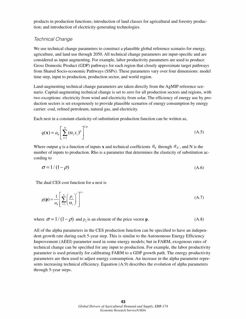
43 Global Drivers of Agricultural Demand and Supply, ERR-174
Economic Research Service/USDA
products in production functions; introduction of land classes for agricultural and forestry produc-tion; and introduction of electricity-generating technologies.
Technical Change
We use technical change parameters to construct a plausible global reference scenario for energy, agriculture, and land use through 2050. All technical change parameters are input-specific and are considered as input augmenting. For example, labor productivity parameters are used to produce Gross Domestic Product (GDP) pathways for each region that closely approximate target pathways from Shared Socio-economic Pathways (SSPs). These parameters vary over four dimensions: model time step, input to production, production sector, and world region.
Land-augmenting technical change parameters are taken directly from the AgMIP reference sce-nario. Capital-augmenting technical change is set to zero for all production sectors and regions, with two exceptions: electricity from wind and electricity from solar. The efficiency of energy use by pro-duction sectors is set exogenously to provide plausible scenarios of energy consumption by energy carrier: coal, refined petroleum, natural gas, and electricity.
Each nest in a constant-elasticity-of-substitution production function can be written as,
1/
01
( ) ( )N
i ii
q a xρ
ρ
=
= α
∑x (A.5)
Where output q is a function of inputs x and technical coefficients 0a through Na , and N is the number of inputs to production. Rho is a parameter that determines the elasticity of substitution ac-cording to
1/ (1 )σ ρ= − (A.6)
The dual CES cost function for a nest is
1/
10
1( )
rrNi
i i
pg
a =
= α ∑p
(A.7)
where 1/ (1 )σ ρ= − and pi is an element of the price vector p. (A.8)
All of the alpha parameters in the CES production function can be specified to have an indepen-dent growth rate during each 5-year step. This is similar to the Autonomous Energy Efficiency Improvement (AEEI) parameter used in some energy models; but in FARM, exogenous rates of technical change can be specified for any input to production. For example, the labor productivity parameter is used primarily for calibrating FARM to a GDP growth path. The energy productivity parameters are then used to adjust energy consumption. An increase in the alpha parameter repre-sents increasing technical efficiency. Equation (A.9) describes the evolution of alpha parameters through 5-year steps.
44 Global Drivers of Agricultural Demand and Supply, ERR-174
Economic Research Service/USDA
1
( ) (1 ( ))T
NSTEPij ij ij
ST g Sα α
=
= +∏ (A.9)
T is an integer that represents the model time step, where T=1 during the base year of 2004. Since the model runs in 5-year steps, T=2 represents 2009. If t is the number of years since 2004, then
NSTEPTt ×=
The flexibility provided by non-neutral technical change is used extensively for calibrating a refer-ence scenario in FARM.
Technical change is neutral if all of the alpha parameters from Equation (A.9) change at the same rate. This can also be accomplished by changing only the 0a parameter and leaving the other a parameters constant.
∏=
+=T
S
NSTEPjjj SgT
1000 ))(1()( αα (A.10)
Agricultural Productivity
Each land-using production function (e.g., wheat, rice, coarse grains) has a technical coefficient associated with each land class that varies over time. A reference scenario was constructed for this report using exogenous changes in yield through 2050 provided through the AgMIP project by the International Food Policy Research Institute (IFPRI). These changes in yield were applied only to the land input, as land-augmenting technical change. Crop yield is also influenced in FARM by changes in prices of agricultural products and inputs to agricultural production. Therefore, simulated crop yield in FARM is a combination of exogenous and price-induced effects.
IFPRI has constructed yield projections through 2050 for a reference scenario and eight climate impact scenarios. These scenarios of yield growth are used by 10 global economic modeling teams in AgMIP project, including FARM. The climate impact scenarios are based on output from two climate models and several crop growth models.
Land as an Input to Production
Land use can shift among crops, pasture, and managed forests in response to population growth and changes in income, with behavioral responses determined by price and income elasticities. The GTAP 7 database distributed by Purdue University includes supplemental data on physical quanti-ties from the Food and Agriculture Organization (FAO). The base year is 2004, and the GTAP data set includes a global social accounting matrix with economic values, land cover for aggregate land types, harvested area for eight crop types, and production quantities for five types of field crops. Further, the GTAP data set provides land use by 18 agro-ecological zones (AEZs). See Monfreda et al. (2009) for background on construction of AEZs for GTAP. Lee et al. (2009) provide a descrip-tion of the land use database provided by GTAP. FARM operates with 6 land classes in each region, which are aggregates of the 18 AEZs provided in GTAP land-use data. The six land classes represent area partitioned by length of growing season, which is a function of temperature and water supply.
The FARM production structure with land as an input is shown in figure A.3. Each of 6 land classes allocates land to 1 of 10 land-using production sectors: 5 field crops, 3 other crop types, pasture for ruminant animals, and managed forests. Within each land-using production sector, land from six
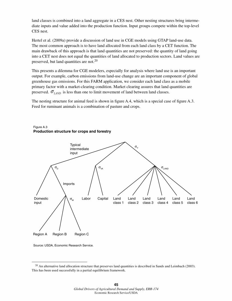
45 Global Drivers of Agricultural Demand and Supply, ERR-174
Economic Research Service/USDA
land classes is combined into a land aggregate in a CES nest. Other nesting structures bring interme-diate inputs and value added into the production function. Input groups compete within the top-level CES nest.
Hertel et al. (2009a) provide a discussion of land use in CGE models using GTAP land-use data. The most common approach is to have land allocated from each land class by a CET function. The main drawback of this approach is that land quantities are not preserved: the quantity of land going into a CET nest does not equal the quantities of land allocated to production sectors. Land values are preserved, but land quantities are not.20
This presents a dilemma for CGE modelers, especially for analysis where land use is an important output. For example, carbon emissions from land-use change are an important component of global greenhouse gas emissions. For this FARM application, we consider each land class as a mobile primary factor with a market-clearing condition. Market clearing assures that land quantities are preserved. LANDσ is less than one to limit movement of land between land classes.
The nesting structure for animal feed is shown in figure A.4, which is a special case of figure A.3. Feed for ruminant animals is a combination of pasture and crops.
20 An alternative land allocation structure that preserves land quantities is described in Sands and Leimbach (2003). This has been used successfully in a partial equilibrium framework.
Source: USDA, Economic Research Service.
Figure A.3
Production structure for crops and forestry
Imports
σY
σD
σM
σVA σLAND
Region A Region B Region C
Domesticinput
Typical intermediateinput
Land class 1
Land class 2
Land class 3
Land class 4
Land class 5
Land class 6
CapitalLabor

46 Global Drivers of Agricultural Demand and Supply, ERR-174
Economic Research Service/USDA
Substitution elasticities in FARM
Four types of substitution elasticities are used in the FARM generic production structure. These elasticities are listed in table A.3 for primary and secondary agricultural products. Primary agri-culture consists of eight crops or crop types, ruminant animals, non-ruminant animals, and dairy. Secondary agriculture consists of crops or animal products processed for final consumption. These elasticities are constant over time and across world regions.
Mσ is an Armington elasticity that determines the substitutability of the same type of product im-ported from other world regions. Dσ is an Armington elasticity that distinguishes domestic prod-ucts from the Armington import aggregate. The GTAP 7 database includes suggested values for Mσ and Dσ , which vary by product. These elasticities are all greater than 1, with some much greater than 1. For FARM, we have set these elasticities to be the same across products but within the range of elasticities suggested by GTAP.
For primary agriculture, we have split the value-added nest into two parts: one nest for labor and capital and the other nest for land inputs (fig. A.3). For this reason, values of VAσ in FARM are not directly comparable to suggested values in the GTAP data set. LANDσ equals 0.4 in all production structures that use land. Yσ then becomes the parameter that determines substitution between land and other inputs. In the ruminant feed production structure (fig. A.4), FEEDσ is set to 1.5 to allow substitution between pasture and feed crops.
Source: USDA, Economic Research Service.
Figure A.4
Feed production structure for ruminant animals
Imports
σD
σM
σLAND
Region A
Oil seeds
Region B Region C
Domesticinput
Coarsegrains
Land class 1
Land class 2
Land class 3
Land class 4
Land class 5
Land class 6
σFEED

47 Global Drivers of Agricultural Demand and Supply, ERR-174
Economic Research Service/USDA
Income and own-price elasticities of demand in FARM
Income and own-price elasticities for consumers are derived from the Linear Expenditure System (LES) and are set indirectly through LES parameters. Unlike substitution elasticities, income and own-price elasticities vary by world region and over time. Income elasticities and own-price elastici-ties for the fourth model time step (year 2019) are shown in tables A.4 and A.5, respectively.
Income elasticities for all agricultural products are very low in developed countries such as the United States. Income elasticities for developing countries are greater but converge over time toward elasticities in the United States. These elasticities are set using modeler’s judgment to be qualita-tively consistent with Muhammad et al. (2011).21
Once income elasticities are set in the LES, no degrees of freedom remain and own-price elasticities of demand follow immediately (table A.5). If the value share of consumption is small for a commod-ity, then the own-price elasticity of demand is close to the income elasticity of demand in absolute value.22
21 The GTAP project provides a set of target income elasticities that are much higher for meat and processed food, even for the United States.
22 GTAP also has a set of target price elasticities by commodity and world region. However, some combinations of GTAP income and own-price elasticities are impossible using the Linear Expenditure System.
Table A.3
Substitution elasticities in the Future Agricultural Resources Model (FARM)
sigma(Y) sigma(VA) sigma(D) sigma(M)
Paddy rice 0.20 0.80 2.00 4.00
Wheat 0.20 0.80 2.00 4.00
Other grains 0.20 0.80 2.00 4.00
Vegetables, fruits, nuts 0.20 0.80 2.00 4.00
Oil seeds 0.20 0.80 2.00 4.00
Sugarcane, sugar beet 0.20 0.80 2.00 4.00
Plant-based fibers 0.20 0.80 2.00 4.00
Other crops 0.20 0.80 2.00 4.00
Cattle, sheep, goats 0.80 0.40 2.00 4.00
Nonruminant animals 0.80 0.40 2.00 4.00
Raw milk 0.80 0.40 2.00 4.00
Bovine meat products 0.00 0.40 2.00 4.00
Other meat products 0.00 0.40 2.00 4.00
Vegetable oils and fats 0.00 0.40 2.00 4.00
Dairy products 0.00 0.40 2.00 4.00
Processed rice 0.00 0.40 2.00 4.00
Sugar 0.00 0.40 2.00 4.00
Other food products 0.00 0.40 2.00 4.00
Beverages and tobacco 0.00 0.40 2.00 4.00

48 Global Drivers of Agricultural Demand and Supply, ERR-174
Economic Research Service/USDA
Table A.4
Income elasticities of demand in the Future Agricultural Resources Model, 2019
USA BrazilFormer Soviet
UnionIndia China
Paddy rice 0.00 0.00 0.00 0.21 0.32
Wheat 0.00 0.27 0.30 0.30 0.40
Other grains 0.00 0.26 0.28 0.25 0.40
Vegetables, fruits, nuts 0.16 0.26 0.29 0.24 0.32
Oil seeds 0.15 0.27 0.29 0.24 0.00
Sugarcane, sugar beet 0.00 0.00 0.31 0.23 0.00
Plant-based fibers 0.15 0.26 0.31 0.25 0.00
Other crops 0.16 0.27 0.00 0.24 0.00
Cattle, sheep, goats 0.15 0.27 0.30 0.00 0.42
Nonruminant animals 0.15 0.27 0.30 0.29 0.41
Raw milk 0.15 0.35 0.30 0.27 0.00
Bovine meat products 0.16 0.32 0.41 0.51 0.30
Other meat products 0.15 0.31 0.40 0.00 0.26
Vegetable oils and fats 0.16 0.30 0.43 0.34 0.24
Dairy products 0.16 0.32 0.39 0.45 0.29
Processed rice 0.16 0.32 0.40 0.41 0.22
Sugar 0.16 0.37 0.42 0.32 0.25
Other food products 0.16 0.34 0.40 0.41 0.26
Beverages and tobacco 0.22 0.40 0.40 0.45 0.30

49 Global Drivers of Agricultural Demand and Supply, ERR-174
Economic Research Service/USDA
Table A.5
Own-price elasticities of demand in the Future Agricultural Resources Model, 2019
USA BrazilFormer Soviet
UnionIndia China
Paddy rice 0.00 0.00 0.00 -0.16 -0.29
Wheat 0.00 -0.24 -0.24 -0.22 -0.36
Other grains 0.00 -0.24 -0.23 -0.18 -0.36
Vegetables, fruits, nuts -0.14 -0.23 -0.23 -0.18 -0.29
Oil seeds -0.14 -0.24 -0.23 -0.18 0.00
Sugarcane, sugar beet 0.00 0.00 -0.25 -0.17 0.00
Plant-based fibers -0.14 -0.24 -0.25 -0.18 0.00
Other crops -0.14 -0.24 0.00 -0.18 0.00
Cattle, sheep, goats -0.14 -0.24 -0.24 0.00 -0.38
Nonruminant animals -0.14 -0.25 -0.24 -0.21 -0.37
Raw milk -0.14 -0.31 -0.24 -0.20 0.00
Bovine meat products -0.14 -0.29 -0.33 -0.37 -0.27
Other meat products -0.14 -0.28 -0.32 0.00 -0.24
Vegetable oils and fats -0.15 -0.27 -0.34 -0.25 -0.22
Dairy products -0.15 -0.29 -0.31 -0.33 -0.26
Processed rice -0.15 -0.29 -0.32 -0.30 -0.20
Sugar -0.15 -0.34 -0.34 -0.23 -0.22
Other food products -0.15 -0.30 -0.32 -0.30 -0.23
Beverages and tobacco -0.20 -0.36 -0.32 -0.33 -0.27

50 Global Drivers of Agricultural Demand and Supply, ERR-174
Economic Research Service/USDA
Appendix B. Decomposition Methodology
A change in a multiplicative relationship can be decomposed into additive components using loga-rithms. In this case, the change is over time, but the decomposition can also be calculated between two scenarios at a point in time. We use the logarithmic mean Divisia index (LMDI) as described by Ang (2005) to decompose changes in supply and demand of agricultural products into explanatory components. For each agricultural product, supply equals area times yield, and demand equals popu-lation times per capita consumption. The demand component for per capita consumption is renamed “income” in this report.
YieldAreaSupply ×=
yieldareaT SSSSSupply ∆+∆=−=∆ 0 (B.1)
where
−−=∆ 00
0
logloglog Area
AreaSS
SSST
T
T
area (B.2)
−−=∆ 00
0
logloglog Yield
YieldSS
SSST
T
T
yield (B.3)
Demand = Population × Consumption (per-capita)
incomepopulationT DDDDDemand ∆+∆=−=∆ 0
(B.4)
where
−−=∆ 00
0
logloglog Pop
PopDD
DDDT
T
T
population (B.5)
−−=∆ 00
0
logloglog Cons
ConsDD
DDDT
T
T
income (B.6)