Sequential monte carlo methods for multiple target ... · IEEE TRANSACTIONS ON SIGNAL PROCESSING, VOL. 50, NO. 2, FEBRUARY 2002 309 Sequential Monte Carlo Methods for Multiple Target

IEEE TRANSACTIONS ON SIGNAL PROCESSING, VOL. 50, NO. 2, FEBRUARY 2002 309

Sequential Monte Carlo Methods for Multiple TargetTracking and Data Fusion

Carine Hue, Jean-Pierre Le Cadre, Member, IEEE, and Patrick Pérez

Abstract—The classical particle filter deals with the estimationof one state process conditioned on a realization of one observationprocess. We extend it here to the estimation of multiple state pro-cesses given realizations of several kinds of observation processes.The new algorithm is used to track with success multiple targets ina bearings-only context, whereas a JPDAF diverges. Making useof the ability of the particle filter to mix different types of observa-tions, we then investigate how to join passive and active measure-ments for improved tracking.

Index Terms—Bayesian estimation, bearings-only tracking,Gibbs sampler, multiple receivers, multiple targets tracking,particle filter.

I. INTRODUCTION

M ULTITARGET tracking (MTT) deals with the state esti-mation of an unknown number of moving targets. Avail-

able measurements may both arise from the targets, if they aredetected, and from clutter. Clutter is generally considered to bea model describing false alarms. Its (spatio–temporal) statisticalproperties are quite different from those of the target, whichmakes the extraction of target tracks from clutter possible. Toperform multitarget tracking, the observer has at his disposal ahuge amount of data, possibly collected on multiple receivers.Elementary measurements are receiver outputs, e.g., bearings,ranges, time-delays, Dopplers, etc.

The main difficulty, however, comes from the assignment ofa given measurement to a target model. These assignments aregenerally unknown, as are the true target models. This is a neatdeparture from classical estimation problems. Thus, two distinctproblems have to be solvedjointly: the data association and theestimation.

As long as the association is considered in a deterministicway, the possible associations must be exhaustively enumerated.This leads to an NP-hard problem because the number of pos-sible associations increases exponentially with time, as in themultiple hypothesis tracker (MHT) algorithm [28]. In the jointprobabilistic data association filter (JPDAF) [11], the associa-tion variables are considered to be stochastic variables, and oneneeds only to evaluate the association probabilities at each timestep. However, the dependence assumption on the associationsimplies the exhaustive enumeration of all possible associations

Manuscript received January 31, 2001; revised October 11, 2001. The asso-ciate editor coordinating the review of this paper and approving it for publicationwas Dr. Petar M. Djuric´.

C. Hue is with Irisa/Université de Rennes 1, Rennes, France (e-mail:[email protected]).

J.-P. Le Cadre is with Irisa/CNRS, Rennes, France (e-mail: [email protected]).P. Pérez is with Microsoft Research, Cambridge, U.K. (e-mail: pperez@mi-

crosoft.com).Publisher Item Identifier S 1053-587X(02)00571-8.

at the current time step. When the association variables are in-stead supposed to be statistically independent like in the prob-abilistic MHT (PMHT [12], [32]), the complexity is reduced.Unfortunately, the above algorithms do not cope with nonlinearmodels and non-Gaussian noises.

Under such assumptions (stochastic state equation and non-linear state or measurement equation non-Gaussian noises), par-ticle filters are particularly appropriate. They mainly consist ofpropagating a weighted set of particles that approximates theprobability density of the state conditioned on the observations.Particle filtering can be applied under very general hypotheses,is able to cope with heavy clutter, and is very easy to implement.Such filters have been used in very different areas for Bayesianfiltering under different names: The bootstrap filter for targettracking in [15] and the Condensation algorithm in computer vi-sion [20] are two examples, among others. In the earliest studies,the algorithm was only composed of two periods: The particleswere predicted according to the state equation during the pre-diction step; then, their weights were calculated with the likeli-hood of the new observation combined with the former weights.A resampling step has rapidly been added to dismiss the parti-cles with lower weights and avoid the degeneracy of the particleset into a unique particle of high weight [15]. Many ways havebeen developed to accomplish this resampling, whose final goalis to enforce particles in areas of high likelihood. The frequencyof this resampling has also been studied. In addition, the use ofkernel filters [19] has been introduced to regularize the sum ofDirac densities associated with the particles when the dynamicnoise of the state equation was too low [26]. Despite this longhistory of studies, in which the ability of particle filter to trackmultiple posterior modes is claimed, the extension of the par-ticle filter to multiple target tracking has progressively receivedattention only in the five last years. Such extensions were firstclaimed to be theoretically feasible in [2] and [14], but the ex-amples chosen only dealt with one single target. In computervision, a probabilistic exclusion principle has been developedin [24] to track multiple objects, but the algorithm is very de-pendent of the observation model and is only applied for twoobjects. In the same context, a Bayesian multiple-blob tracker(BraMBLe) [6] has just been proposed. It deals with a varyingnumber of objects that are depth-ordered thanks to a 3-D statespace. Lately, in mobile robotic [29], a set of particle filters foreach target connected by a statistical data association has beenproposed. We propose here a general algorithm for multitargettracking in the passive sonar context and take advantage of itsversatility to extend it to multiple receivers.

This work is organized as follows. In Section II, we recallthe principles of the basic particle filter with adaptive resam-pling for a single target. We begin Section III with a presentationof the multitarget tracking problem and its classical solutions

1053–587X/02$17.00 © 2002 IEEE

310 IEEE TRANSACTIONS ON SIGNAL PROCESSING, VOL. 50, NO. 2, FEBRUARY 2002

and of the related work on multitarget tracking by particle fil-tering methods. Then, we present our multitarget particle filter(MTPF). The new algorithm combines the two major steps (pre-diction and weighting) of the classical particle filter with a Gibbssampler-based estimation of the assignment probabilities. Then,we propose to add two statistical tests to decide if a target hasappeared or disappeared from the surveillance area. Carryingon with the approach of the MTPF, we finally present an exten-sion to multireceiver data in the context of multiple targets (theMRMTPF). Section IV is devoted to experiments. Simulationresults in a bearings-only context with a variable clutter den-sity validate the MTPF algorithm. A comparison with a JPDAFbased on the extended Kalman filter establishes the superiorityof the MTPF for the same scenario. Then, a simulation with oc-clusion shows how the disappearance of a target can be handled.The suitable quantity and distribution of active measurementsare then studied in a particular scenario to improve the perfor-mance obtained with passive measurements only.

As far as the notational conventions are concerned, we alwaysuse the index to refer to one among the tracked targets. Theindex designates one of the observations obtained at instant. The index is devoted to the particles. The index is used

for indexing the iterations in the Gibbs sampler, andis usedfor the different receivers. Finally, the probability densities aredenoted by if they are continuous and byif they are discrete.

II. BASIC SINGLE-TARGET PARTICLE FILTER

For the sake of completeness, the basic particle filter is nowbriefly reviewed. We consider a dynamic system represented bythe stochastic process , whose temporal evolutionis given by the state equation:

(1)

It is observed at discrete times via realizations of the stochasticprocess governed by the measurement model

(2)

The two processes and in (1) and (2)are only supposed to be independent white noises. Note that thefunctions and are not assumed linear. We will denote by

the sequence of the random variables and byone realization of this sequence. Note that throughout the

paper, the first subscript of any vector will always refer to thetime.

Our problem consists of computing at each timethe condi-tional density of the state , given all the observations ac-cumulated up to, i.e., andof estimating any functional of the state by the expecta-tion as well. The recursive Bayesian filter, whichis also called the optimal filter, resolves exactly this problem intwo steps at each time.

Suppose we know . The prediction stepis done ac-cording to the following equation:

(3)

The observation enables us to correct this prediction usingBayes’s rule:

(4)

Under the specific assumptions of Gaussian noisesandand linear functions and , these equations lead to theKalman filter’s equations. Unfortunately, this modeling is notappropriate in many problems in signal and image processing,which makes the calculation of the integrals in (3) and (4)infeasible (no closed-form).

The original particle filter, which is called the bootstrapfilter [15], proposes to approximate the densitiesby a finiteweighted sum of Dirac densities centered on elements of

, which are called particles.The application of the bootstrap filter requires that one knows

how to do the following:

• sample from initial prior marginal ;• sample from for all ;• compute for all through a known

function such that , wheremissing normalization must not depend on.

The algorithm then evolves the particle set, where is the particle and

its weight, such that the density can be approximated bythe density . In the bootstrap filter, theparticles are “moved” by sampling from the dynamics (1), andimportance sampling theory shows that the weighting is onlybased on likelihood evaluations. In the most general setting[9], the displacement of particles is obtained by samplingfrom an appropriate density, which might depend on thedata as well. The complete procedure is summarized in Fig. 1.Some convergence results of the empirical distributions to theposterior distribution on the path space have been proved whenthe number of particles tends toward infinity [25], [10].In the path space , each particle at time can beconsidered to be a discrete path of length . Comparedwith the particle filter presented in Fig. 1, particle filteringin the space of paths consists of incrementing the particlestate space at each time step and representing each particleby the concatenation of the new position at timeand the setof previous positions between times 0 and . In [25], thefluctuations on path space of the so-called interacting particlesystems are studied. In the context of sequential Monte Carlomethods [10] that cover most of the particle filtering methodsproposed in the last few years, the convergence and the rate ofconvergence of order of the average mean square erroris proved. Under more restrictive hypotheses, the almost-sureconvergence is proved as well [10].

To evaluate the degeneracy of the particle set, the effectivesample size has been defined [21], [23]. As advocated in [9], aresampling step is performed in the algorithm presented in Fig. 1in an adaptive way when the effective sample size, estimated by

, is under a given threshold. It avoids to obtain a degenerate

HUE et al.: SEQUENTIAL MONTE CARLO METHODS FOR MTT AND DATA FUSION 311

Fig. 1. Basic particle filter with adaptive resampling.

particle set composed of only few particles with high weightsand all the others with very small ones.

Beside the discretization of the filtering integrals, the use ofsuch particles enables the maintenance of multiple hypotheseson the position of the target and to keep in the long term onlythe particles whose position is likely given the whole sequenceof observations.

We find more details on the algorithm in [9] or [15] and onadaptive resampling in [9] and [21]. After these recalls, let uspresent briefly the multitarget tracking problem and its clas-sical solutions, as well as the existing works on particle filteringmethods for MTT. Then, we will propose the MTPF.

III. M ULTITARGET PARTICLE FILTER

A. MTT Problem and Its Classical Treatment

Let be the number of targets to track that are assumed tobe known and fixed for the moment (the case of a varying un-known number will be addressed in Section III-C). The indexdesignates one among the targets and is always used as firstsuperscript. Multitarget tracking consists of estimating the statevector made by concatenating the state vectors of all targets. It isgenerally assumed that the targets are moving according to inde-pendent Markovian dynamics. At time,follows the state equation (1) decomposed inpartial equa-tions

(5)

The noises and are supposed only to be white bothtemporally and spatially and independent for .

The observation vector collected at timeis denoted by. The index is used as first superscript to refer

to one of the measurements. The vector is composed ofdetection measurements and clutter measurements. The falsealarms are assumed to be uniformly distributed in the obser-vation area. Their number is assumed to arise from a Poissondensity of parameter , where is the volume of the obser-vation area, and is the number of false alarms per unit volume.As we do not know the origin of each measurement, one has tointroduce the vector to describe the associations between themeasurements and the targets. Each componentis a randomvariable that takes its values among . Thus,

indicates that is associated with theth target. In this case,is a realization of the stochastic process

if (6)

Again, the noises and are supposed only to bewhite noises, independent for . We assume that the func-tions are such that they can be associated with functionalforms such that

We dedicate the model 0 to false alarms. Thus, if ,the th measurement is associated with the clutter, but we donot associate any kinematic model to false alarms.

As the indexing of the measurements is arbitrary, all the mea-surements have the samea priori probability to be associatedwith a given model . At time , these association probabilitiesdefine the vector . Thus,

for , for all isthe discrete probability that any measurement is associated withthe th target.

To solve the data association, some assumptions are com-monly made [3].

A1) One measurement can originate from one target or fromthe clutter.

A2) One target can produce zero or one measurement at onetime.

The assumption A1) expresses that the association is exclusiveand exhaustive. Consequently, .

Assumption A2) implies that may differ from and,above all, that the association variables forare dependent.

Under these assumptions, the MHT algorithm [28] builds re-cursively the association hypotheses. One advantage of this al-gorithm is that the appearance of a new target is hypothesizedat each time step. However, the complexity of the algorithm in-creases exponentially with time. Some pruning solutions mustbe found to eliminate some of the associations.

The JPDAF begins with a gating of the measurements. Onlythe measurements that are inside an ellipsoid around the pre-dicted state are kept. The gating assumes that the measurementsare distributed according to a Gaussian law centered on the pre-dicted state. Then, the probabilities of each associationare estimated. As the variables are assumed dependent by


A2), this computation implies the exhaustive enumeration of allthe possible associations for .

The novelty in the PMHT algorithm [12], [32], [33] consistsof replacing the assumption A2) by A3):

A3) One target can produce zero or several measurements atone time.

This assumption is often criticized because it does not match thephysical reality. However, from a mathematical point of view, itensures the stochastic independence of the variablesand itdrastically reduces the complexity of thevector estimation.

The assumptions A1) and A3) will be kept in the MTPF pre-sented later. Let us present now the existing works solving MTTwith particle filtering methods.

B. Related Work: MTT With Particle Filtering Methods

In the context of multitarget tracking, particle filteringmethods are appealing: As the association needs only to beconsidered at a given time iteration, the complexity of dataassociation is reduced. First, two extensions of the bootstrapfilter have been considered. In [2], a bootstrap-type algorithmis proposed in which the sample state space is a “(multitarget)state space.” However, nothing is said about the associationproblem that needs to be solved to evaluate the sample weights.It is, in fact, the ability of the particle filtering to deal withmultimodality due to (high) clutter that is pointed out comparedwith deterministic algorithms like the nearest neighbor filteror the probabilistic data association (PDA) filter. No exampleswith multiple targets are presented. The simulations only dealwith a single target in clutter with a linear observation model.In [14], a hybrid bootstrap filter is presented where the particlesevolve in a single-object state space. Each particle gives ahypothesis on the state of one object. Thus, thea posteriorilaw of the targets, given the measurements, is represented bya Gaussian mixture. Each mode of this law then correspondsto one of the objects. However, as pointed out in [14], thelikelihood evaluation is possible only under the availability ofthe “prior probabilities of all possible associations between”the measurements and the targets. It may be why the simulationexample only deals with one single target in clutter. Even ifthe likelihood could be evaluated, the way to represent theaposteriori law by a mixture can lead to the loss of one of thetargets during occlusions. The particles tracking an occludedtarget get very small weights and are therefore discarded duringthe resampling step. This fact has been pointed out in [29].

In image analysis, the Condensation algorithm has been ex-tended to the case of multiple objects as well. In [24], the caseof two objects is considered. The hidden state is the concate-nation of the two single-object states and of a binary variableindicating which object is closer to the camera. This latter vari-able solves the association during occlusion because the mea-surements are affected to the foreground object. Moreover, aprobabilistic exclusion principle is integrated to the likelihoodmeasurement to penalize the hypotheses with the two objectsoverlapping. In [6], the state is composed of an integer equal tothe number of objects and of a concatenation of the individualstates. A three-dimensional (3-D) representation of the objects

gives access to their depth ordering, thus solving the associationissue during occlusions. Finally, in mobile robotics [29], a par-ticle filter is used for each object tracked. The likelihood of themeasurements is written like in a JPDAF. Thus, the assignmentprobabilities are evaluated according to the probabilities of eachpossible association. Given these assignment probabilities, theparticle weights can be evaluated. The particle filters are thendependent through the evaluation of the assignment probabili-ties. Independently of the two latter works [6] and [29], we havedeveloped the MTPF, where the data association is approachedin the same probabilistic spirit as the basic PMHT [12], [32].

First, to estimate the density ,with particle filtering methods, we must

choose the state space for the particles. As mentioned before,a unique particle filter with a single-target state space seemedto us a poor choice as the particles tracking an occluded objectwould be quickly discarded. We have considered using oneparticle filter per object but without finding a consistent wayto make them dependent. The stochastic association vectorintroduced in Section III-A could also be considered to be anadditional particle component. However, as the ordering of themeasurements is arbitrary, it would not be possible to devise adynamic prior on it. Moreover, the state space would increase,further making the particle filter less effective. Finally, we havechosen to use particles whose dimension is the sum of thoseof the individual state spaces corresponding to each target, asin [6] and [24]. Each of these concatenated vectors then givesjointly a representation of all targets. Let us describe the MTPF.Further details on the motivations for the different ingredientsof the MTPF can be found in [18].

C. MTPF Algorithm

Before describing the algorithm itself, let us first notice thatthe association probability that a measurement is associatedwith the clutter is a constant that can be computed

(7)

(8)

(9)

where is the number of measurements arising from theclutter at time . Assuming that there areclutter originatedmeasurements among the measurements collected attime , the a priori probability that any measurement comesfrom the clutter is equal to ; hence, we get the equality

used to derive (9) from (8).The initial set of particles is

such that each component for is sampledfrom independently from the others. Assume we haveobtained with .Each particle is a vector of dimension , where we de-note by the th component of and where designatesthe dimension of target.


The prediction is performed by sampling from some proposaldensity . In the bootstrap filter case, coincides with the dy-namics (5)

... (10)

Examine now the computation of the likelihood of the obser-vations conditioned on theth particle. We can write for all

(11)

Note that the first equality in (11) is true only under theassumption of conditional independence of the measure-ments, which we will make. To derive the second equalityin (11), we have used the total probability theorem withthe events and under the supplementaryassumption that the normalization factors betweenand

is the same for all.We still need to estimate at each time step the association

probabilities , which can be seen as the stochasticcoefficients of the -component mixture. Two main ways havebeen found in the literature to estimate the parameters of thismodel: the expectation maximization (EM) method (and its sto-chastic version the SEM algorithm [5]) and the data augmenta-tion method. The second one amounts in fact to a Gibbs sampler.

In [12], [32], and [33], the EM algorithm is extended and ap-plied to multitarget tracking. This method implies that the vec-tors and are considered as parameters to estimate. Themaximization step can be easily conducted in the case of de-terministic trajectories, and the additional use of a maximuma posteriori(MAP) estimate enables the achievement of it fornondeterministic trajectories. Yet, the nonlinearity of the stateand observation functions makes this step very difficult. Finally,the estimation is done iteratively in a batch approach we wouldlike to avoid. For these reasons, we have not chosen an EM al-gorithm to estimate the association probabilities.

The data augmentation algorithm is quite different in its prin-ciple. The vectors , , and are considered to be randomvariables with prior densities. Samples are then obtained iter-atively from their joint posterior using a proper Markov chainMonte Carlo (MCMC) technique, namely, the Gibbs sampler.This method has been studied in [4], [8], [13], [30], and [31],for instance. It can be run sequentially at each time period. TheGibbs sampler is a special case of the Metropolis–Hasting algo-rithm with the proposal densities being the conditional distribu-tions and the acceptance probability being consequently alwaysequal to one. See [7] for an introduction to MCMC simulationmethods and also for a presentation of the EM algorithm.

Let be the stochastic variable associated with the proba-bility . For , the method consists of gener-ating a Markov chain that converges to the stationary distribu-tion , which cannot be sampled directly. For that, wemust get a partition of and to sample alternatively

from the conditional posterior distribution of each component ofthe partition. Let the index denote the iterations in the Gibbssampler. The second subscript of the vectors refers to the itera-tion counter. Assume that the first elements of the Markovchain have been drawn. We sample thecom-ponents of as follows:

......

In our case, at a given instant, we follow this algorithm with

for

for

for

(12)

The initialization of the Gibbs sampler consists of assigning uni-form association probabilities, i.e., for all

, and taking , i.e., the cen-troid of the predicted particle set. The variables do not needinitializing because at the first time step of the Gibbs sampler,they will be sampled conditioned on and

. Then, suppose that at instant, we have already simulated. The th iteration is handled as follows.

• As the are assumed to be independent,their individual discrete conditional density reads

(13)

Assignment variables are discrete, and we can write1

if

if(14)

The realizations of the vector are then sam-pled according to the weights

for

• Mixture proportion vector is drawn from the con-ditional density

Dirichlet (15)

where we denote by the number of equal toand whereDirichlet denotes the Dirichletdistribution on the simplex , ,

1Using Bayes’s rule,p(ajb; c) = (p(bja; c)p(ajc))=p(bjc).


: with density pro-portional to

. The vector is first drawn ac-cording to (15) and then normalized to restore the sum

to .• has to be sampled according to the density

(16)

The values of might imply that one target is as-sociated with zero or several measurements. Let us define

: . Hence, we de-compose the preceding product in two products:

(17)

where , . The first productcontains the targets that are associated with at least onemeasurement under the association . In this case,

the measurements are denoted by . The secondproduct contains the targets that are associated with nomeasurements under .

— Let be an index in the first product. We can write

(18)

We are not able to sample directly from the density

for the same reasons as those exposed in Section II tojustify the use of the particle filter (intractability ofthe integrals). We propose to build the particle set

, , whose weightsmeasure the likelihood of the observations associatedby to target . More precisely, we let

(19)

As the predicted empirical lawis “close” to the predicted law , we ex-pect the empirical distribution

to be close to .However, the weak convergence of to

, when tends toward infinityremains to be proved. Not being able to sample from

, , we draw as a real-ization from .

— Now, let be an index in the second product. As wedo not have any measurement to correct the predictedparticles, we draw a realization from the density

for .After a finite number of iterations, we estimate the vector

by the average of its last realizations:

(20)

Finally, the weights can be computed according to (11) usingthe estimate of . By construction, follows the law

. Thus, the use of a Gibbs sampler enables us totake into account the current measurements. Consequently,the estimates measure in a way thea posteriori detectionprobability of each target. It improves the estimation of thetargets because the measurements contribute to the estimationproportionally to these probabilities . Moreover, thea prioriprobability of detecting a target, which is usually denoted by

, is not needed in the MTPF. This probability is needed whenthe associations are considered in classical algorithms like thePMHT or the JPDAF.

The resampling step is performed in an adaptive way whenthe estimated effective sample size is under the threshold

. In [18], we have compared the performance ofparticle filtering with systematic and adaptive resampling ina single-object bearings-only synthetic example. The bias onthe estimation error was almost the same, but the standarddeviation was twice as small using adaptive resampling ratherthan systematic resampling.

Due to the estimation of the vector needed for the compu-tation of the particles likelihood, the convergence of the MTPFcould be affected. It could be interesting to evaluate the error onthe estimate of implied by the error made on the estimate of

. This is not addressed in this work.The complete procedure is summarized in Fig. 2.

D. Varying Number of Targets

Until now, the number of targets was assumed known andconstant. We now make suggestions to relax this constraint. Asper the disappearance of objects, the vectorprovides usefulinformation: the disappearance of one target from the surveil-lance area can be detected by a drop in the correspondingcomponent. We will use the estimate of to decide betweenthe two following hypotheses.

• —The target is present in the surveillance area.• —The target is not present in the surveillance area.

If the target is still present in the surveillance area, the fall ofcan only be due to its nondetection, which occurs with a

probability . Let be the binary variable equal to 1 ifthe th target has been detected at timeand 0 otherwise. Overa test interval and for a given target, the variables

are distributed according to a binomial law of


Fig. 2. MTPF: Particle filter algorithm for multiple targets with adaptive resampling.

parameters . These variables are unknown, but wecan use the estimates to estimate them. Let us define

if

otherwise(21)

where is a probability threshold. The test withthe obtained variables decides on the true hy-pothesis. This test consists of computing the distance

between the expected size and theobtained size of each class (here, the class 0 and the class 1).When tends toward infinity, is asymptotically distributedas a law. One admits that is reasonably approximated by a

law under the conditions that the expected size of each class

is higher than 4. That is why in practice, the length of the in-terval must be chosen such that .

As far as the algorithm is concerned, this reduction only leadsto update (the number of targets) and to remove the compo-nents of the particles related to the disappeared target. It can beintegrated to the MTPF as described in Fig. 3.

On the other hand, the arrival of a new target might be relatedto an observation whose likelihood is low, whatever target it isassociated with. As a result, assignment variables simulated bythe Gibbs sampler might be more often equal to 0. We proposeto use the values of the assignment variables to decide betweenthe two following hypotheses.

• —A new target is arriving inside the surveillancearea.

• —No new target is arriving inside the surveillancearea.


Fig. 3. Particle filter algorithm for multiple targets with adaptive resampling and varying target number.

Let be the estimate of , which is the number of measure-ments arising from the clutter at time, supplied by the Gibbssampler

(22)

where . Over an interval ,a test enables us to measure the adequation between thePoisson law of parameter followed by andthe empirical law of the variables . This test canalso be integrated to the MTPF, as described in Fig. 3. Neverthe-less, the initialization of the new target based on the observationsets is a tricky problem, which we have not solved yet.

E. Multireceiver Multitarget Particle Filter—MRMTPF

A natural extension of the MTPF is to consider that ob-servations can be collected by multiple receivers. Letbetheir number. We will see that we can easily adapt the particlefilter to this situation. We always consider that the targets(their number is fixed again) obey the state equation (5). Some

useful notations must be added to modify the measurementequations. The observation vector at timewill be denotedby , where refers to the receiverthat received the th measure. This measurement is then arealization of the stochastic process

if (23)

We assume the independence of the observations collected bythe different receivers. We denote by the functions

that are proportional to . Thelikelihood of the observations conditioned by theth particle isreadily obtained as

(24)


There is no strong limitation on the use of the particle filterfor multireceiver and multitarget tracking: the MRMTPF is ob-tained from the MTPF by replacing the likelihood functions

by the functions .Moreover, it can deal with measurements of varied periodic-

ities. We present in Section IV-B a scenario mixing active andpassive measurements.

IV. SIMULATIONS RESULTS

For all the following simulations, the burn-in period of theGibbs sampler has been fixed to and the totalnumber of iterations to . The resampling thresholdhas been fixed to .

A. Application to Bearings-Only Problems With Clutter

To illustrate theMTPF algorithm, we first deal with classicalbearings-only problems with three targets. In the context of aslowly maneuvering target, we have chosen a nearly-constant-velocity model (see [22] for a review of the principal dynamicalmodels used in this domain).

1) Model and the First Scenario Studied:The state vectorsrepresent the coordinates and the velocities in the– plane:

for . For each target, thediscretized state equation associated with time periodis

(25)

where is the identity matrix in dimension 2, and isa Gaussian zero-mean vector with covariance matrix

. Let be the estimate of computed by the particle

filters with , i.e., .A set of measurements is available at discrete times and

can be divided in two subsets.

• A subset of “true” measurements that follow (26). A mea-surement produced by theth target is generated accordingto

(26)

where is a zero-mean Gaussian noise with covarianceindependent of , and and are the Cartesian

coordinates of the observer, which are known. We assumethat the measurement produced by one target is availablewith a detection probability .

• A subset of “false” measurements whose number followsa Poisson distribution with mean , where is the meannumber of false alarms per unit volume. We assume thesefalse alarms are independent and uniformly distributedwithin the observation volume .

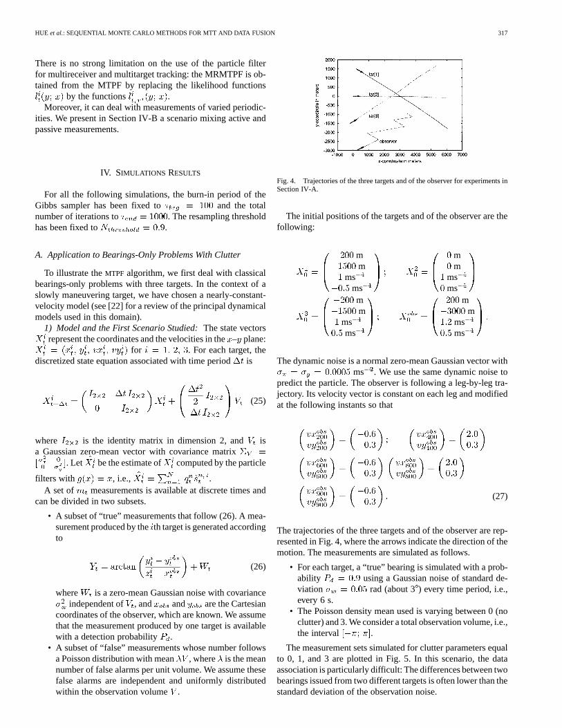
Fig. 4. Trajectories of the three targets and of the observer for experiments inSection IV-A.

The initial positions of the targets and of the observer are thefollowing:

mm

msms

mm

msms

mm

msms

mm

msms

The dynamic noise is a normal zero-mean Gaussian vector withms . We use the same dynamic noise to

predict the particle. The observer is following a leg-by-leg tra-jectory. Its velocity vector is constant on each leg and modifiedat the following instants so that

(27)

The trajectories of the three targets and of the observer are rep-resented in Fig. 4, where the arrows indicate the direction of themotion. The measurements are simulated as follows.

• For each target, a “true” bearing is simulated with a prob-ability using a Gaussian noise of standard de-viation rad (about 3) every time period, i.e.,every 6 s.

• The Poisson density mean used is varying between 0 (noclutter) and 3. We consider a total observation volume, i.e.,the interval .

The measurement sets simulated for clutter parameters equalto 0, 1, and 3 are plotted in Fig. 5. In this scenario, the dataassociation is particularly difficult: The differences between twobearings issued from two different targets is often lower than thestandard deviation of the observation noise.


Fig. 5. Measurements simulated with a detection probabilityP = 0:9. (a)�V = 0. (b)�V = 1. (c)�V = 3.

2) Results of the MTPF:First, the initialization of the par-ticle set has been done according to a Gaussian law whose meanvector and covariance matrix are

mm

msms

mm

msms

mm

msms

(28)

and

for

(29)To evaluate the performance of the algorithm according to theclutter density, we have performed different runs of theMTPF with 1000 particles for . The scenariois the same for each run, i.e., the true target trajectories andthe simulated measurements are identical. At each time, thebias and the standard deviation for theth component of aredefined by

bias

std (30)

To avoid the compensation of elementary bias of opposite signs,we average the absolute values of the biasbias . Then, wedefine, for each target, and for theth component

bias bias (31)

and we average the standard deviations

std std (32)

These different quantities, which are normalized by their valuesobtained with no clutter, are plotted against the clutter param-eter in Fig. 6. Except for the and components of the thirdtarget, the standard deviation is not very sensitive to clutter. InFig. 7, the MTPF estimate averaged over the 20 runs have beenplotted with the confidence ellipsoid on position given by

. In particular, the component of the third targetseems well estimated, which counterbalances the variations ob-served in Fig. 6.

The ellipsoids plotted in Fig. 7 represent the variance over the20 runs of the posterior mean estimates and enable us to assessthe variance of the MTPF estimator for particles. Theposterior covariance of the estimate from one particular run isalso a useful indicator to assess the quality of the estimation.The confidence ellipsoids corresponding to the covarianceof the posterior estimate are presented for one particular run inFig. 8(a). As the covariance of dynamic noise is not very highand especially as the prior at time zero is narrow, one might thinkthat the estimates obtained without measurements2 could be asgood. However, the posterior covariance obtained without usingthe measurements increase a lot as presented in Fig. 8(b).

With a Pentium III 863 MHz, particles, a burn-inperiod , and a total amount of itera-tions in the Gibbs sampler, it takes around 1 s per time step tocompute the MTPF estimate of three targets with bearings-onlymeasurements.

The next section shows the ability of the MTPF to recoverfrom a poor initialization.

3) Effect of a Highly Shifted Initialization:The initial posi-tions and velocities of the objects are the same as in the previoussection. The observer is still following a leg-by-leg trajectory,but its initial position is now

mm

msms

Its velocity vector is constant on each leg and modified at thefollowing instants so that

2Such estimates are obtained by applying the prediction step and by givingconstant weights to the particles instead of computing them given the measure-ments.


Fig. 6. Bias, resp. std, for clutter parameter= 1; 2; 3 over bias, resp. std, obtained with no clutter obtained with 1000 particles for 20 runs. (a) Bias onx andyposition for the three targets. (b) Bias onvx andvy position for the three targets. (c) std onx andy position for the three targets. (d) std onvx andvy positionfor the three targets.

Fig. 7. Averaged MTPF estimate of the posterior means (dashed lines) over 20 runs and associated2� confidence ellipsoids for the three targets withN = 1000

particles and with a detection probabilityP = 0:9. (a)�V = 0. (b)�V = 1. (c)�V = 2. (d)�V = 3. The solid lines are the true trajectories.

(33)

The trajectories of the three targets and of the observer are rep-resented in Fig. 9. Compared with the previous section, the firstmaneuver occurs earlier to make the targets resolvable earlier.The initialization of the particle set has been done according toa Gaussian law whose mean vector and covariance ma-


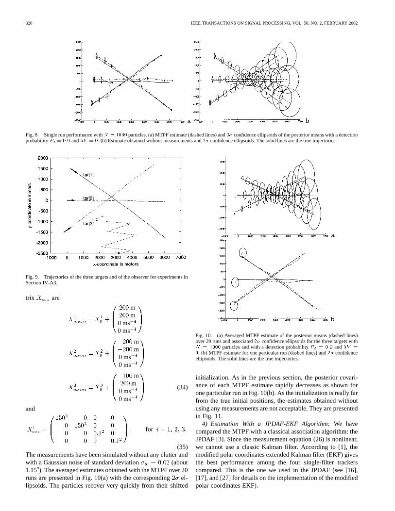
Fig. 8. Single run performance withN = 1000 particles. (a) MTPF estimate (dashed lines) and2� confidence ellipsoids of the posterior means with a detectionprobabilityP = 0:9 and�V = 0. (b) Estimate obtained without measurements and2� confidence ellipsoids. The solid lines are the true trajectories.

Fig. 9. Trajectories of the three targets and of the observer for experiments inSection IV-A3.

trix are

mm

msms

mm

msms

mm

msms

(34)

and

for

(35)The measurements have been simulated without any clutter andwith a Gaussian noise of standard deviation (about1.15 ). The averaged estimates obtained with the MTPF over 20runs are presented in Fig. 10(a) with the correspondingel-lipsoids. The particles recover very quickly from their shifted

Fig. 10. (a) Averaged MTPF estimate of the posterior means (dashed lines)over 20 runs and associated2� confidence ellipsoids for the three targets withN = 1000 particles and with a detection probabilityP = 0:9 and�V =

0. (b) MTPF estimate for one particular run (dashed lines) and2� confidenceellipsoids. The solid lines are the true trajectories.

initialization. As in the previous section, the posterior covari-ance of each MTPF estimate rapidly decreases as shown forone particular run in Fig. 10(b). As the initialization is really farfrom the true initial positions, the estimates obtained withoutusing any measurements are not acceptable. They are presentedin Fig. 11.

4) Estimation With a JPDAF-EKF Algorithm:We havecompared the MTPF with a classical association algorithm: theJPDAF [3]. Since the measurement equation (26) is nonlinear,we cannot use a classic Kalman filter. According to [1], themodified polar coordinates extended Kalman filter (EKF) givesthe best performance among the four single-filter trackerscompared. This is the one we used in the JPDAF (see [16],[17], and [27] for details on the implementation of the modifiedpolar coordinates EKF).


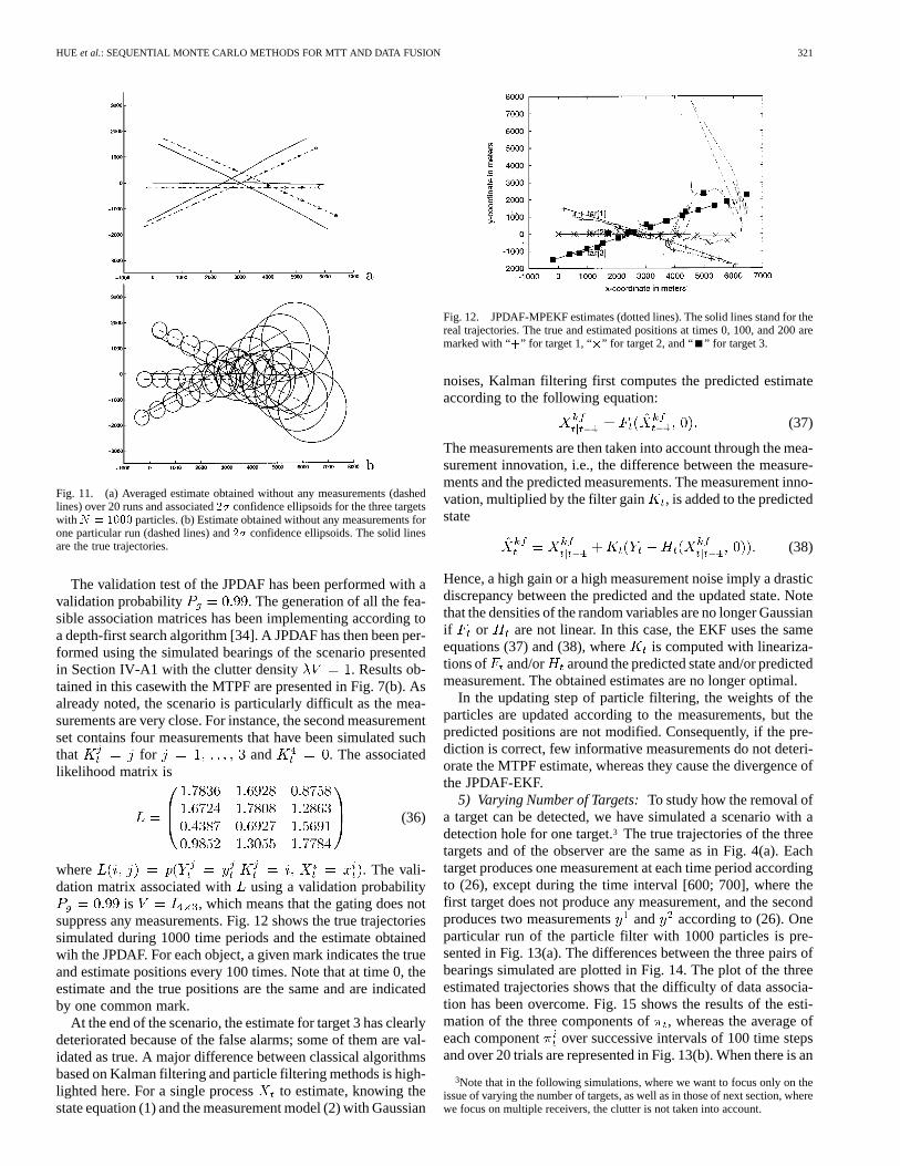
Fig. 11. (a) Averaged estimate obtained without any measurements (dashedlines) over 20 runs and associated2� confidence ellipsoids for the three targetswithN = 1000 particles. (b) Estimate obtained without any measurements forone particular run (dashed lines) and2� confidence ellipsoids. The solid linesare the true trajectories.

The validation test of the JPDAF has been performed with avalidation probability . The generation of all the fea-sible association matrices has been implementing according toa depth-first search algorithm [34]. A JPDAF has then been per-formed using the simulated bearings of the scenario presentedin Section IV-A1 with the clutter density . Results ob-tained in this casewith the MTPF are presented in Fig. 7(b). Asalready noted, the scenario is particularly difficult as the mea-surements are very close. For instance, the second measurementset contains four measurements that have been simulated suchthat for and . The associatedlikelihood matrix is

(36)

where . The vali-dation matrix associated with using a validation probability

is , which means that the gating does notsuppress any measurements. Fig. 12 shows the true trajectoriessimulated during 1000 time periods and the estimate obtainedwih the JPDAF. For each object, a given mark indicates the trueand estimate positions every 100 times. Note that at time 0, theestimate and the true positions are the same and are indicatedby one common mark.

At the end of the scenario, the estimate for target 3 has clearlydeteriorated because of the false alarms; some of them are val-idated as true. A major difference between classical algorithmsbased on Kalman filtering and particle filtering methods is high-lighted here. For a single process to estimate, knowing thestate equation (1) and the measurement model (2) with Gaussian

Fig. 12. JPDAF-MPEKF estimates (dotted lines). The solid lines stand for thereal trajectories. The true and estimated positions at times 0, 100, and 200 aremarked with “+” for target 1, “�” for target 2, and “ ” for target 3.

noises, Kalman filtering first computes the predicted estimateaccording to the following equation:

(37)

The measurements are then taken into account through the mea-surement innovation, i.e., the difference between the measure-ments and the predicted measurements. The measurement inno-vation, multiplied by the filter gain , is added to the predictedstate

(38)

Hence, a high gain or a high measurement noise imply a drasticdiscrepancy between the predicted and the updated state. Notethat the densities of the random variables are no longer Gaussianif or are not linear. In this case, the EKF uses the sameequations (37) and (38), where is computed with lineariza-tions of and/or around the predicted state and/or predictedmeasurement. The obtained estimates are no longer optimal.

In the updating step of particle filtering, the weights of theparticles are updated according to the measurements, but thepredicted positions are not modified. Consequently, if the pre-diction is correct, few informative measurements do not deteri-orate the MTPF estimate, whereas they cause the divergence ofthe JPDAF-EKF.

5) Varying Number of Targets:To study how the removal ofa target can be detected, we have simulated a scenario with adetection hole for one target.3 The true trajectories of the threetargets and of the observer are the same as in Fig. 4(a). Eachtarget produces one measurement at each time period accordingto (26), except during the time interval [600; 700], where thefirst target does not produce any measurement, and the secondproduces two measurementsand according to (26). Oneparticular run of the particle filter with 1000 particles is pre-sented in Fig. 13(a). The differences between the three pairs ofbearings simulated are plotted in Fig. 14. The plot of the threeestimated trajectories shows that the difficulty of data associa-tion has been overcome. Fig. 15 shows the results of the esti-mation of the three components of, whereas the average ofeach component over successive intervals of 100 time stepsand over 20 trials are represented in Fig. 13(b). When there is an

3Note that in the following simulations, where we want to focus only on theissue of varying the number of targets, as well as in those of next section, wherewe focus on multiple receivers, the clutter is not taken into account.


Fig. 13. (a) Target trajectories and their estimate with 1000 particles. (b) Average of the estimated components of the vector� over the consecutive ten timeintervals of length 100 and over 20 trials.

Fig. 14. Differences between the three pairs of target bearings at each time period compared with the standard deviation of the observation noise. (a)Measurements1 and 2. (b) Measurements 1 and 3. (c) Measurements 2 and 3.

Fig. 15. Estimated components of the vector� obtained with 1000 particles. (a)̂� . (b) �̂ . (c) �̂ .

ambiguity about the origin of the measurements (i.e., when thedifferences between the bearings are lower than the standard de-viation noise), the components ofvary in average around onethird for targets, and they stabilize at uniform estimates(one third for targets) when the ambiguity disappears.The momentary measurement gap for the first target is correctlyhandled as the first component is instantaneously estimatedas 0.15 from instant 600 to 700.

B. Application to Problems With Active and PassiveMeasurements

In the following scenario, we consider two targets and oneobserver whose trajectories are plotted in Fig. 16(a). The initialpositions are

mm

msms

mm

msms

mm

msms

The difference between the two simulated bearings is very oftenlower than the measurement noise std as shown in Fig. 16(b).In the following simulations, all the particle clouds have beeninitialized around the true positions with the covariance matrix

defined in (29). In addition, the observer does not follow aleg-by-leg trajectory. This makes the estimation of the trajecto-ries quite difficult, and a lot of runs of the MTPF lost the track.Consequently, the standard deviation over 20 runs increases a lotthrough time, as illustrated by Fig. 16(d). To improve trackingperformance, we study the impact of adding active measure-ments (here, ranges). We assume that noisy ranges are availableperiodically during time intervals of lengthwith period , i.e.,these measurements are present at timeif .A noisy range associated with theth target is supposed to followthe equation

(39)

where is a Gaussian noise with standard deviation, where . This noise modeling

seems more realistic than the constant standard deviation mod-eling generally used in such contexts. For instance, forand , the simulated ranges of the two targets are shown


Fig. 16. (a) Trajectories of the targets and of the observer. (b) Difference between the noisy bearings associated with the targets compared with the standarddeviation of the measurement noise= 0:05, i.e., 2.8�. (c) Noisy ranges simulated forT = 30 andP = 100. (d)–(f) Averaged estimates (dashed lines) and2� confidence ellipsoids obtained with bearings measurements and 0%, 20%, and 50% of range measurements, respectively. The solid lines stand for the realtrajectories.

in Fig. 16(c). The evolution of the bias and the standard devia-tion of the estimation errors has been studied according to thequantity of active measurements on the one hand and to theirtemporal distribution on the other.

1) Quantity of Active Measurements:For these experimen-tations, we have fixed and taken .Fig. 17 summarizes the evolution of the bias and the standard de-viation of the estimation errors as a function of the active mea-surement percentage. Fig. 16(e) and (f) shows the MRMTPFestimated posterior means averaged over 20 runs and theconfidence ellipsoids with, respectively, 20% and 50% of ac-tive measurements.

First, the addition of active measurements particularly im-proves the estimation of the componentsand for the twotargets. Fig. 16(d)–(f) also shows the drastic reduction of the sizeof the confidence ellipsoids along the-axis when range mea-surements are added. Theand -positions of the two targetsare actually very close, and the bearings measurements do nothelp to dissociate the targets because of the difficulty of dataassociation. However, as the difference between the-positions

of the two targets is very high, the range measurements are verydifferent. They thus help a lot to distinguish the targets and tosolve the data association.

The percentage of 20% of active measurements appears to bea good compromise between a significant improvement of theestimation and a reasonable quantity of active measurements.

With a Pentium III 863 MHz, particles, a burn-inperiod , and a total amount of itera-tions in the Gibbs sampler, it takes around 840 ms per time stepto compute the MTPF estimates of two targets with bearingsmeasurements and 20% of range measurements.

2) Temporal Distribution of Active Measurements:We nowlook at the impact of the temporal distribution of the activemeasurements: the ratio of passive over active measurementsis fixed to 5 (i.e., to 20% of active measurements). The intervallengths considered are and . The averagedMRMTPF estimates and the confidence ellipsoids obtainedwith 20 runs and 1000 particles are represented in Fig. 18 fordifferent values. First of all, if the state evolution was deter-ministic, the better choice would be to consider active measure-


Fig. 17. Bias on the estimation of the hidden states(x; y; v ; v ) of the two targets with 1000 particles over 20 runs. (a) Bias onx andy. (b) Bias onvx andvy.

Fig. 18. AveragedMRMTPFestimates (dotted lines) and2� confidence ellipsoids (dashed lines) with 1000 particles: (a)T = 10,P = 50; (b)T = 20,P = 100;(c) T = 40, P = 200; (d) T = 100, P = 500. The solid lines are the true trajectories.

ments at the beginning and at the end of the scenario. In our case,the state evolution is stochastic. We observe that the bias is in-dependent of the temporal distribution of range measurements.The size of the confidence ellipsoids increases with. Theactive measurements should then be available as frequently aspossible to improve the estimation performance.

V. CONCLUSION

Two major extensions of the classical particle filter have beenpresented in order to deal first with multiple targets (MTPF) andthen with multiple receivers (MRMTPF). Considering the dataassociation from a stochastic point of view, Gibbs sampling isthe workhorse for estimating association vectors, thus avoidingcombinatorial drawbacks. Moreover, the particle filtering per-forms satisfactorily, even in the presence of dense clutter. A nextstep would be to deal with more realistic clutter models. Twostatistical tests have also been proposed for detecting changes

of the target states (emitting or not). Even if the MTPF is quiteversatile, it can suffer from initialization problems. This draw-back cannot be completely avoided in the multitarget context.This will be addressed in future studies. Finally, MTPF has beenextended to multiple receivers and multiple measurements (herepassive and active). In this context, the effects of the temporaldistribution of active measurement have been investigated. Pre-liminary results on this aspect show all the importance of mea-surement scheduling.

REFERENCES

[1] S. Arulampalam, “A comparison of recursive style angle-only target mo-tion analysis algorithms,” Electron. Surveillance Res. Lab., Salisbury,Australia, Tech. Rep. DSTO-TR-0917, Jan. 2000.

[2] D. Avitzour, “Stochastic simulation Bayesian approach to multitargetapproach,”Proc. Inst. Elect. Eng.—Radar, Sonar, Navigat., vol. 142, no.2, pp. 41–44, Apr. 1995.

[3] Y. Bar-Shalom and T. E. Fortmann,Tracking and Data Associa-tion. New York: Academic, 1988.


[4] G. Casella and E. I. George, “Explaining the Gibbs sampler,”Amer.Statist., vol. 46, no. 3, pp. 167–174, 1992.

[5] G. Celeux and J. Diebolt, “A stochastic approximation type EM algo-rithm for the mixture problem,”Stochast. Stochast. Rep., vol. 41, pp.119–134, 1992.

[6] J. Mac Cormick and M. Isard, “Bramble: A Bayesian multiple-blobtracker,” inProc. 8th Int. Conf. Comput. Vision, vol. 2, Vancouver, BC,Canada, July 9–12, 2001, pp. 34–41.

[7] J. F. G. de Freitas, “Bayesian methods for neural networks,” Ph.D. dis-sertation, Trinity College, Univ. Cambridge, Cambridge, U.K., 1999.

[8] J. Diebolt and C. P. Robert, “Estimation of finite mixture distributionsthrough Bayesian sampling,”J. R. Statist. Soc. B, vol. 56, pp. 363–375,1994.

[9] A. Doucet, “On sequential simulation-based methods for Bayesian fil-tering,” Signal Process. Group, Dept. Eng., Cambridge, U.K., Tech. Rep.CUED/F-INFENG/TR 310, 1998.

[10] , “Convergence of sequential Monte Carlo methods,” SignalProcess. Group, Dept. Eng., Cambridge, U.K., Tech. Rep. CUED/F-IN-FENG/TR 381, 2000.

[11] T. E. Fortmann, Y. Bar-Shalom, and M. Scheffe, “Sonar tracking of mul-tiple targets using joint probabilistic data association,”IEEE J. OceanicEng., vol. OE-8, pp. 173–184, July 1983.

[12] H. Gauvrit, J.-P. Le Cadre, and C. Jauffret, “A formulation of multitargettracking as an incomplete data problem,”IEEE Trans. Aerosp. Electron.Syst., vol. 33, pp. 1242–1257, Oct. 1997.

[13] A. E. Gelfand and A. F. M. Smith, “Sampling-based approaches to calcu-lating marginal densities,”J. Amer. Statist. Assoc., vol. 85, pp. 398–409,1990.

[14] N. Gordon, “A hybrid bootstrap filter for target tracking in clutter,”IEEETrans. Aerosp. Electron. Syst., vol. 33, pp. 353–358, Jan. 1997.

[15] N. Gordon, D. Salmond, and A. Smith, “Novel approach to non-linear/non-Gaussian Bayesian state estimation,”Proc. Inst. Elect. Eng.F, Radar Signal Process., vol. 140, no. 2, pp. 107–113, April 1993.

[16] W. Grossman, “Bearings-only tracking: A hybrid coordinate system ap-proach,”J. Guidance, Contr., Dynamics, vol. 17, no. 3, pp. 451–457,May/June 1994.

[17] J. C. Hassab,Underwater Signal and Data Processing. Boca Raton,FL: CRC, 1989, pp. 221–243.

[18] C. Hue, J.-P. Le Cadre, and P. Pérez, “Tracking multiple objects withparticle filtering,” IRISA, Rennes, France, Tech. Rep., Oct. 2000.

[19] M. Hürzeler and H. R. Künsch, “Monte Carlo approximations for gen-eral state space models,”J. Comput. Graph. Statist., vol. 7, pp. 175–193,1998.

[20] M. Isard and A. Blake, “CONDENSATION—Conditional density prop-agation for visual tracking,”Int. J. Comput. Vis., vol. 29, no. 1, pp. 5–28,1998.

[21] A. Kong, J. S. Liu, and W. H. Wong, “Sequential imputation method andBayesian missing data problems,”J. Amer. Statist. Assoc., vol. 89, pp.278–288, 1994.

[22] X. Li and V. Jilkov, “A survey of maneuvering target tracking: Dynamicmodels,” inProc. Conf. Signal Data Process. Small Targets, Orlando,FL, Apr. 2000.

[23] J. S. Liu, “Metropolized independent sampling with comparison to re-jection sampling and importance sampling,”Statist. Comput., vol. 6, pp.113–119, 1996.

[24] J. MacCormick and A. Blake, “A probabilistic exclusion principle fortracking multiple objects,” inProc. 7th Int. Conf. Comput. Vis., Kerkyra,Greece, Sept. 20–27, 1999, pp. 572–578.

[25] P. Del Moral and A. Guionnet, “Central limit theorem for nonlinear fil-tering and interacting particle systems,”Ann. Appl. Probab., vol. 9, no.2, pp. 275–297, 1999.

[26] C. Musso and N. Oudjane, “Particle methods for multimodal filtering,”in Proc. 2nd IEEE Int. Conf. Inform. Fusion, Silicon Valley, CA, July6–8, 1999.

[27] N. Peach, “Bearings-only tracking using a set of range parameterisedextended Kalman filters,”Proc. Inst. Elect. Eng. Contr. Theory Appl.,vol. 142, no. 1, Jan. 1995.

[28] D. Reid, “An algorithm for tracking multiple targets,”IEEE Trans. Au-tomat. Contr., vol. 24, no. AC-6, pp. 84–90, 1979.

[29] D. Schulz, W. Burgard, D. Fox, and A. B. Cremers, “Tracking multiplemoving targets with a mobile robot using particle filters and statisticaldata association,” inProc. IEEE Int. Conf. Robotics Automat., Seoul,Korea, May 21–26, 2001, pp. 1665–1670.

[30] A. Smith and G. Roberts, “Bayesian computation via the Gibbs Samplerand related Markov chain Monte Carlo methods,”J. R. Statist. Soc., B,vol. 55, no. 1, pp. 3–24, 1993.

[31] M. Stephens, “Bayesian methods for mixtures of normal distributions,”Ph.D. dissertation, Magdalen College, Oxford Univ., Oxford, U.K.,1997.

[32] R. L. Streit and T. E. Luginbuhl, “Maximum likelihood method for prob-abilistic multi-hypothesis tracking,”Proc. SPIE, vol. 2235, Apr. 5–7,1994.

[33] P. Willett, Y. Ruan, and R. Streit, “The PMHT for maneuvering targets,”Proc. SPIE, vol. 3373, Apr. 1998.

[34] B. Zhou, “Multitarget tracking in clutter: Fast algorithms for data asso-ciation,” IEEE Trans. Aerosp. Electron. Syst., vol. 29, pp. 352–363, Apr.1993.

Carine Hue was born in 1977. She received the M.Sc. degree in mathematicsand computer science in 1999 from the University of Rennes, Rennes, France.Since 1999, she has been pursuing the Ph.D. degree with IRISA, Rennes, andworks on particle filtering methods for tracking in signal processing and imageanalysis.

Jean-Pierre Le Cadre(M’93) received the M.S. degree in mathematics in 1977and the “Doctorat de 3eme cycle” degree in 1982 and the “Doctorat d’Etat”degree in 1987, both from INPG, Grenoble, France.

From 1980 to 1989, he was with the Groupe d’Etudes et de Recherche enDetection Sous-Marine (GERDSM), which is a laboratory of the Directiondes Constructions Navales (DCN), mainly on array processing. In thisarea, he conducted both theoretical and practical researches (towed arrays,high-resolution methods, performance analysis, etc.). Since 1989, he has beenwith IRISA/CNRS, where is “Directeur de Recherche.” His interests have nowmoved toward other topics like system analysis, detection, multitarget tracking,data association, and operations research.

Dr. Le Cadre received (with O. Zugmeyer) the Eurasip Signal Processing bestpaper award in 1993.

Patrick Pérez was born in 1968. He graduated from Ecole Centrale Paris,France, in 1990. He received the Ph.D. degree in signal processing andtelecommunications from the University of Rennes, Rennes, France, in 1993.

After one year as an INRIA post-doctoral fellow at Brown University,Providence, RI, he was appointed a Full Time INRIA researcher. In 2000, hejoined Microsoft Research, Cambridge, U.K. His research interests includeprobabilistic models for image understanding, high-dimensional inverse prob-lems in image analysis, analysis of motion, and tracking in image sequences.

Documents

Sequential monte carlo methods for multiple target ... · IEEE TRANSACTIONS ON SIGNAL PROCESSING, VOL. 50, NO. 2, FEBRUARY 2002 309 Sequential Monte Carlo Methods for Multiple Target