Embed Size (px)
Citation preview

Convergence of Sequential Monte Carlo Methods
by
Dan Crisan‡ - Arnaud Doucet†*
‡Statistical Laboratory, DPMMS,
University of Cambridge, 16 Mill Lane,
Cambridge, CB2 1SB, UK.
Email: [email protected]
†Signal Processing Group, Engineering Department,
University of Cambridge, Trumpington Street,
Cambridge CB2 1PZ, UK.
Email: [email protected]
*corresponding author.
1

Abstract
Bayesian estimation problems where the posterior distribution evolves over time through the accumulation
of data arise in many applications in statistics and related fields. Recently, a large number of algorithms
and applications based on sequential Monte Carlo methods (also known as particle filtering methods) have
appeared in the literature to solve this class of problems; see (Doucet, de Freitas & Gordon, 2001) for a
survey. However, few of these methods have been proved to converge rigorously. The purpose of this paper
is to address this issue.
We present a general sequential Monte Carlo (SMC) method which includes most of the important features
present in current SMC methods. This method generalizes and encompasses many recent algorithms. Under
mild regularity conditions, we obtain rigorous convergence results for this general SMC method and therefore
give theoretical backing for the validity of all the algorithms that can be obtained as particular cases of it.
Keywords: Bayesian estimation, Filtering, Markov chain Monte Carlo, Nonlinear non Gaussian state
space model, Sequential Monte Carlo.
2

1 Introduction
Many real-world data analysis tasks involve estimating unknown quantities when only partial or inaccu-
rate observations are available. In most of these applications, prior knowledge of the underlying system is
available. This knowledge allows us to adopt a Bayesian approach to the problem; that is, to start with
a prior distribution for the unknown quantities and a likelihood function relating these quantities to the
observations. Within this setting, one performs inference on the unknown quantities based on the posterior
distribution. Often, the observations arrive sequentially in time and one is interested in estimating recur-
sively in time the evolving posterior distribution. This problem is known sometimes as the Bayesian or
optimal filtering problem. It has many applications in statistics and related areas such as automatic control,
econometrics, machine learning and signal processing.
Except in a few special cases, including linear Gaussian state space models, the posterior distributions
cannot be obtained analytically. For over thirty years, many approximation schemes, such as the extended
Kalman filter and Gaussian sum approximations, have been proposed to surmount this problem (West &
Harrison, 1997). However, in many realistic problems, these approximating methods are unreliable. Standard
iterative algorithms such as Markov chain Monte Carlo (MCMC) methods are also ineffective as the posterior
distribution evolves over time (Robert & Casella, 1999).
Recently, there has been a surge of interest in SMC methods for solving sequential Bayesian estimation
problems. These methods utilize a random sample (or particle) based representation of the posterior prob-
ability distributions. The particles are propagated over time using a combination of sequential importance
sampling, selection/resampling and MCMC steps. Following the paper of Gordon, Salmon and Smith (1993)
introducing the so-called bootstrap filter, see (Kitagawa, 1996; Isard & Blake, 1998; West, 1993a; West,
1993b) for related early work, many improved SMC methods have been proposed; see for example (Berzuini,
Best, Gilks & Larizza, 1997; Doucet, Godsill & Andrieu, 2000; Doucet, de Freitas & Gordon, 2001; Gilks &
3

Berzuini, 1999; Hurzeler & Kunsch, 1998; Liu & Chen, 1998; Pitt & Shephard, 1999; Tanizaki, 1996). These
algorithms mainly rely on improved importance sampling/resampling strategies and MCMC steps.
Of all the algorithms available, the most extensively studied is the bootstrap filter (Gordon, Salmond &
Smith, 1993), also known as the interacting particle systems/resolution algorithm; see (Del Moral, 1996; Del
Moral, 1997) and subsequent papers. In (Crisan, Del Moral & Lyons, 1999), a rigorous treatment is given to
a whole class of SMC methods. This class of methods does not however include most of the characteristics
of standard methods commonly used by practitioners (Doucet, de Freitas & Gordon, 2001).
The aim of this paper is to present and study rigourously a general SMC method that includes most of
these characteristics. The following are the main new features presented in this paper:
• We remove the standard assumptions that the signal process is Markov and that the observations are
conditionally independent upon the signal in order to include the methods presented in (Liu & Chen,
1998).
• The importance sampling step is done using a general transition kernel which can depend on both the
observations and the current Monte Carlo approximation of the posterior distribution.
• The conditions imposed on the resampling step are less restrictive - for example, the unbiasedness
assumption is lifted.
• An MCMC step is added after the resampling procedure in order to address the problem of sample
depletion. This method, originally proposed by Gilks & Berzuini (1999), is generalized by allowing the
MCMC kernel to depend on the whole population of particles.
• The convergence results are given on the path space, that is, we prove the convergence not to the
posterior distribution of the current state of the signal, but to the posterior distribution of the whole
trajectory of the signal.
4
Under suitable regularity conditions on the dynamic model of interest, the importance sampling function,
the selection scheme and the MCMC kernel used, we prove convergence of the empirical distribution of
particles produced by the SMC method to the posterior distribution of the signal as the number of particles
increases. The techniques used in this paper are close in spirit to those in (Crisan, Del Moral & Lyons,
1999), although the aims and the results are different. For a newcomer to this field, we recommend reading
(Crisan, 2001) first.
As stated in the abstract, many algorithms presented in the literature (Carpenter, Clifford & Fearnhead,
1999; Chen & Liu, 2000; Doucet, Godsill & Andrieu, 2000; Gilks & Berzuini, 1999; Gordon, Salmond &
Smith, 1993; Liu & Chen, 1998) are particular cases of the method presented here and, therefore, receive
rigorous treatment in this paper. It is worth noting that a straightforward adaptation of those proofs would
also allow rigourous convergence results to be obtained for other SMC algorithms such as the auxiliary particle
filter (Pitt & Shephard, 1999) and also for some Monte Carlo algorithms developed in statistical physics
such as Quantum Monte Carlo and Transfer Matrix Monte Carlo; see (Iba, 2000) for a brief description of
these methods and their connections to the ones presented here.
The rest of the paper is organized as follows: In Section 2, the model and estimation objectives are given.
In Section 3, the SMC algorithm is described and its different steps are detailed. The links with previous
methods are briefly discussed. In Section 4, simple sufficient conditions are given to ensure asymptotic
convergence of the empirical measures toward their true values. The rate of convergence of the average mean
square error is also established. In Section 5, we apply these results to an algorithm developed to perform
speech enhancement. All the proofs are given in the Appendix.
2 Problem Statement
Let (Ω, F, P ) be a probability space on which we have defined two vector-valued stochastic processes X =
Xt, t ∈ N and Y = Yt, t ∈ N∗. The process X is usually called the signal process and the process Y is
5

called the observation process. Let nx and ny be the dimensions of the state space of X and of Y . We will
denote by Xi:j and Yi:j the path of the signal and of the observation process from time i to time j,
Xi:j , (Xi, Xi+1, ..., Xj) , Yi:j , (Yi, Yi+1, ..., Yj) .
Let xi:j and yi:j be generic points in the space of paths of the signal and observation processes,
xi:j , (xi, xi+1, ..., xj) ∈ (Rnx )j−i+1
, yi:j , (yi, yi+1, ..., yj) ∈ (Rny )j−i+1
.
The signal process X satisfies X0 ∼ π0 (dx0) and evolves according to the following equation,
Pr (Xt ∈ At|Y0:t−1 = y0:t−1, X0:t−1 = x0:t−1) =
∫
At
kt (y0:t, x0:t−1, dxt) , At ∈ B (Rnx ) (1)
where kt (y0:t, x0:t−1, dxt) is a probability transition kernel
kt : P((Rnx )
t)−→ P
((Rnx )
t+1)
(ktµ) (dx0:t) = kt (y0:t, x0:t−1, dxt) µ (dx0:t−1) .
P((Rnx )
t+1)
and P((Rnx )
t)
respectively represent the set of probability measures defined on B((Rnx )
t+1),
the Borel σ−algebra on (Rnx )t+1
and on B((Rnx )
t), the Borel σ−algebra on (Rnx )
t. The observation
process Y satisfies
Pr (Yt ∈ Bt|Y0:t−1 = y0:t−1, X0:t = x0:t) =
∫
Bt
gt (y0:t, x0:t) dyt, Bt ∈ B (Rny ) . (2)
We assume that the sequence (πt, ρt)t∈N satisfies the following recurrence formula:
Bayes’ recursion. For all t ≥ 0 and Ai ∈ B (Rnx ) , i = 0, ..., t, A0:t = A0 × · · · ×At, we have
Prediction ρt (A0:t) =∫
A0:t−1kt (y0:t, x0:t−1, At)πt−1 (dx0:t−1)
Updating πt (A0:t) = C−1t
∫A0:t
gt (y0:t, x0:t) ρt (dx0:t) ,
where Ct is a normalizing constant Ct , ∫(Rnx)t+1 gt (y0:t, x0:t) ρt (dx0:t).
6

If µ is a measure, f is a function and K is a Markov kernel, we use the following standard notation
(µ, f) , ∫ fdµ, µK (A) , ∫ µ (dx) K (A|x) , Kf (x) , ∫ K (dz|x) f (z) .
Using this notation, if ft : (Rnx )t+1 → R, then the recurrence formula implies that, for all t ∈ N,
Prediction (ρt, ft) = (πt−1, ktft)
Updating (πt, ft) = (ρt, ftgt) (ρt, gt)−1
.
(3)
Remark 1 Let X be a Markov process with respect to the filtration Ft , σ (Xs, Ys, s ∈ 0, . . . , t) with
transition kernel
ht (A, xt−1) , P (Xt ∈ A|Xt−1 = xt−1) , A ∈ B (Rnx ) , xt−1 ∈ Rnx .
Also, assume that P(Yt ∈ dyt|F−
t
)= P (Yt ∈ dyt|Xt), where F−
t , σ (Xs, Ys, s ∈ 0, . . . , t− 1 , Xt) and for
all xt ∈ Rnx , the conditional distribution of Yt given the event Xt = xt is absolutely continuous with
respect to the Lebesgue measure, that is there exists i (yt, xt) such that for any xt−1 ∈ Rnx
P (Yt ∈ dyt|Xt = xt) = i (yt, xt) dyt.
Then the sequence (πt, ρt)t∈N satisfies the Bayes’ recursion condition with kt , ht and gt , it.
Except for a very restricted number of dynamic models, it is impossible to evaluate the joint posterior
distribution πt in a closed form expression. In the next section, we present a SMC method to solve this
problem.
3 A Sequential Monte Carlo Method
3.1 Algorithm
A SMC method is a recursive algorithm which produces, at each time t, a cloud of particles whose empirical
measure closely “follows” the distribution πt. The particles reside in the state space of πt, hence in the space
7

(Rnx )t+1
. Note that the dimension of the space where the particles live increases in time: at time t it is
equal to (t + 1)nx. One can view the particles as (discrete) paths of length t + 1 units in Rnx (the signal’s
space).
We describe a general algorithm which generates at time t (for all t > 0) N particles/pathsx
(i)0:t
N
i=1
with an associated empirical measure πNt
πNt (dx0:t) , 1
N
N∑
i=1
δx(i)0:t
(dx0:t)
that is “close” to πt. The algorithm is recursive in the sense thatx
(i)0:t
N
i=1is produced using the observation
obtained at time t and the previous set of particlesx
(i)0:t−1
N
i=1produced at time t − 1 (whose empirical
measure πNt−1 was “close” to πt−1).
We also introduce a transition kernel Ξt (y0:t, x0:t−1, πt−1, dx0:t) which is used in order to obtain an
intermediate set of particles x(i)0:t. We denote by ρt the resulting importance distribution
ρt , πt−1Ξt.
We assume that ρt is absolutely continuous with respect to ρt and let ht be the strictly positive Radon
Nykodym derivative dρt
dρt= ht, where ht (·) = ht (y0:t, πt−1, ·). Then πt is also absolutely continuous with
respect to ρt and
dπt
dρt
∝ gtht. (4)
We also assume that we can sample exactly from π0 at t = 0. The algorithm proceeds as follows.
At time t = 0.
Step 0: Initialization
• For i = 1, ..., N , sample x(i)0 ∼ π0 (dx0) and set t = 1.
At time t ≥ 1,
Step 1: Importance Sampling step
8

• For i = 1, ..., N , sample x(i)0:t ∼ Ξt
(y0:t, x
(i)0:t−1, π
Nt−1, dx0:t
).
• For i = 1, ..., N , evaluate the normalized importance weights w(i)t
w(i)t ∝ gt
(y0:t, x
(i)0:t
)ht
(y0:t, π
Nt−1, x
(i)0:t
)(5)
and let ρNt and πN
t be the measures
ρNt (dx0:t) , 1
N
N∑
i=1
δex(i)0:t
(dx0:t) , (6)
πNt (dx0:t) , N∑
i=1
w(i)t δex(i)
0:t(dx0:t) . (7)
Step 2: Selection step
• Multiply/Discard particlesx
(i)0:t
N
i=1with respect to high/low importance weights w
(i)t to obtain N particles
x
(i)0:t
N
i=1. Let πN
t denote the associated empirical measure
πNt (dx0:t) , 1
N
N∑
i=1
δx(i)0:t
(dx0:t) . (8)
Step 3: MCMC step
• For i = 1, ..., N , sample x(i)0:t ∼ Kt
(x
(j)0:t
N
j=1, dx0:t
)where Kt (·, ·) is a Markov kernel of invariant
distribution πt (dx0:t). Let πNt denote the associated empirical measure
πNt (dx0:t) , 1
N
N∑
i=1
δx(i)0:t
(dx0:t) . (9)
• Set t← t + 1 and go to Step 1.
3.2 Implementation Issues
We now detail the various steps of the method.
Importance Sampling Step
9

The new set of particles/paths is obtained by sampling from Ξt
(y0:t, x
(i)0:t−1, π
Nt−1, dx0:t
), which, obviously,
depends on πNt−1, the observations y0:t and on the current paths
x
(i)0:t−1
N
i=1. The new paths
x
(i)0:t
N
i=1are
then distributed approximately according to ρt (dx0:t); ρt (dx0:t) being chosen to be “as close as possible” to
πt (dx0:t). There are unlimited choices for Ξt
(y0:t, x
(i)0:t−1, πt−1, dx0:t
), the only condition is that the weights
w(i)t given by (5) are well-defined and can be computed analytically.
Most of the algorithms presented in the literature are such that
Ξt
(y0:t, x
(i)0:t−1, π
Nt−1, dx0:t
)= δ
x(i)0:t−1
(dx0:t−1) Ξt
(y0:t, x
(i)0:t−1, π
Nt−1, dxt
),
that is, the new path x(i)0:t is obtained by keeping the current path x
(i)0:t−1 and extending it by adding a new
point x(i)t , where x
(i)t is sampled from Ξt
(y0:t, x
(i)0:t−1, π
Nt−1, dxt
). We now discuss several possible choices
for Ξt
(y0:t, x
(i)0:t−1, π
Nt−1, dxt
). A sensible selection criterion is to choose a proposal that minimises the
conditional variance of the importance weights at time t, given x(i)0:t−1 and y0:t. According to this strategy,
it has been shown that the optimal distribution is P(
dxt| y0:t, x(i)0:t−1
)(Doucet, Godsill & Andrieu, 2000).
• Optimal sampling distribution. If we sample x(i)t according to
P(
dxt| y0:t, x(i)0:t−1
)∝ gt
(y0:t, x
(i)0:t−1, xt
)kt
(y0:t, x
(i)0:t−1, dxt
)
then the importance weight is equal to
w(i)t ∝
∫gt
(y0:t, x
(i)0:t−1, xt
)kt
(y0:t, x
(i)0:t−1, dxt
).
If this integral does not admit an analytical expression, one has to use an alternative method.
• Prior distribution. If we use the prior distribution kt
(y0:t, x
(i)0:t−1, dxt
)as importance distribution, the
importance weight is proportional to gt
(x
(i)0:t, x
(i)t , y0:t
). However, as underlined in (Pitt & Shephard, 1999),
this strategy is sensitive to outliers.
• Likelihood distribution. Assume the likelihood gt
(y0:t, x
(i)0:t−1, xt
)is integrable in argument xt, that is
∫gt
(y0:t, x
(i)0:t−1, xt
)dxt <∞,
10

then one can sample x(i)t according to
Ξt
(y0:t, x
(i)0:t−1, π
Nt−1, dxt
)∝ gt
(y0:t, x
(i)0:t−1, xt
)
and
w(i)t ∝ kt
(y0:t, x
(i)0:t−1, xt
).
This is useful when the observation noise is very low as the likelihood is then usually very peaked compared
to the prior distribution kt
(y0:t, x
(i)0:t−1, dxt
); see (Fox, Thrun, Burgard & Dellaert, 2001) for an alternative
algorithm to handle a low observation noise level.
• Alternative sampling distribution. It is possible to design a variety of alternative sampling distributions
(Doucet, Godsill & Andrieu, 2000; Pitt & Shephard, 1999). For example, one can use the results of a subop-
timal deterministic algorithm to construct an importance sampling distribution Ξt
(y0:t, x
(i)0:t−1, π
Nt−1, dxt
).
This is very useful in applications where P(
dxt| y0:t, x(i)0:t−1
)is too expensive or impossible to use and
kt
(y0:t, x
(i)0:t−1, dxt
)is inefficient.
Resampling Step
The aim of the resampling/selection step is to obtain an “unweighted” empirical distribution approxima-
tion πNt (dx0:t) of the weighted measure πN
t (dx0:t). A selection procedure associates a number of offspring
N(i)t ∈ N with each particle
x
(i)0:t
N
i=1, where
∑Ni=1 N
(i)t = N , to obtain N new particles
x
(i)0:t
N
i=1with
associated empirical distribution πNt , where
πNt (dx0:t) = N−1
N∑
i=1
N(i)t δex(i)
0:t(dx0:t) = N−1
N∑
i=1
δx(i)0:t
(dx0:t) .
We briefly describe three classes of selection schemes. All can be implemented in O (N) iterations.
• Sampling Importance Resampling (SIR)/Multinomial Sampling procedure. This procedure, introduced
originally by (Gordon, Salmond & Smith, 1993), is the most popular. One samples N times from πNt (dx0:t)
to obtain
x(i)0:t
N
i=1. This is equivalent to jointly drawing
N
(i)t
N
i=1according to a multinomial distribution
11

of parameters N and w(i)t . It is possible to implement the SIR procedure exactly in O (N) operations
using a classical algorithm (Ripley, 1987). In this case, we have E(N
(i)t
)= Nw
(i)t and var
(N
(i)t
)=
Nw(i)t
(1− w
(i)t
).
• Residual Resampling (Higuchi, 1997; Liu & Chen, 1998). Set N(i)t =
⌊Nw
(i)t
⌋, then perform a SIR proce-
dure to select the remaining N t = N−∑Ni=1 N
(i)t samples with the new weights w
′(i)t = N
−1
t
(w
(i)t N − N
(i)t
).
Finally, add the results to the current N(i)t . In this case, we again obtain E
(N
(i)t
)= Nw
(i)t but var
(N
(i)t
)=
N tw′(i)t
(1− w
′(i)t
).
• Minimal Variance Sampling. This class includes the stratified/systematic sampling procedures introduced
in (Carpenter, Clifford & Fearnhead, 1999; Kitagawa, 1996) where a set U of N points is generated in the
interval [0, 1], each of the points a distance N−1 apart. The number N(i)t is taken to be the number of
points in U that lie between∑i−1
j=1 w(j)t and
∑ij=1 w
(j)t . It also includes the Tree Based Branching algorithm
presented in (Crisan, 2001). If we denoteNw
(i)t
, Nw(i)t −
⌊Nw
(i)t
⌋, then the variance of all the algorithms
in this class is var(N
(i)t
)=Nw
(i)t
(1−
Nw
(i)t
).
Actually, as we will discuss later on, it is not necessary to design unbiased selection schemes, that is we
can have E(N
(i)t
)6= Nw
(i)t . An example of a biased selection scheme is the deterministic selection scheme
proposed by Kitagawa (1996).
MCMC Step
If the distribution of the importance weights is highly skewed then the particles x(i)0:t which have high impor-
tance weights w(i)t are selected many times and, thus, numerous particles x
(i)0:t will have identical positions.
This amounts to a depletion of samples. One way to perform sample regeneration consists of considering a
mixture approximation (Gordon, Salmond & Smith, 1993; Liu & West, 2001). An alternative method based
on an MCMC procedure has recently been proposed in (Gilks & Berzuini, 1999). The rationale behind
the use of the MCMC method is based on the following remark. Assume that the particlesx
(i)0:t
N
i=1are
12

distributed marginally according to πt (dx0:t). Then, if we apply to each particle x(i)0:t a Markov transition
kernel Kt
(x
(i)0:t, dx0:t
)of invariant distribution πt (dx0:t), the new particles
x
(i)0:t
N
i=1are still distributed
according to the posterior distribution of interest. One can use any of the standard MCMC methods
(Metropolis-Hastings, Gibbs sampler, etc.). Moreover, unlike for standard MCMC applications (Robert &
Casella, 1999), we do not require that the kernel is ergodic1. For example, one can use a Gibbs sampling
step which updates at time t the values of the process xt from time t − L + 1 to t, i.e., we sample x(i)k for
k = t− L + 1, . . . , t according to P (dxk|Y0:t, x(i)0:k−1, x
(i)k+1:t).
Further, one can allow the Markov transition kernel to be dependent on the whole population of particles
x
(i)0:t
N
i=1, provided it satisfies
∫Kt
(x
(i)0:t
N
i=1, dx0:t
) N∏
i=1
πt
(dx
(i)0:t
)= πt (dx0:t) .
This way one can use the information provided by the whole set of particles so as to design, for example, an
efficient proposal for a Metropolis-Hastings sampler.
4 Convergence Study
Let B (Rn ) and Cb (Rn ) respectively be the space of bounded, Borel measurable functions and the space of
bounded continuous functions on Rn . We denote ‖f‖ , supx∈Rn
|f (x)|. In this section, we first establish the
convergence (and the rate of convergence) to 0 of the average mean square error E[((
πNt , ft
)− (πt, ft)
)2]
for any ft ∈ B((Rnx )
t+1)
under quite general conditions (where the expectation is over all the realizations
of the random particle methods). Then we prove the (almost sure) convergence of πNt towards πt under
more restrictive conditions.
From now on we will assume that the observation process is fixed to a given observation record Yt = yt,
t > 0. All the convergence results will be proven under this condition.
1Note that it does not need to be Markov either but in practice it is usually limited to this case.
13
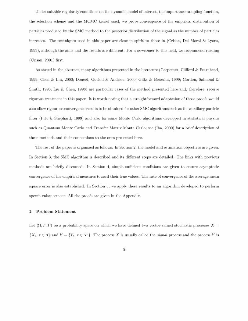
4.1 Bounds for mean square errors
Let us consider the following assumptions.
Assumptions.
1. -A. Importance distribution and weights.
• ρt is assumed absolutely continuous with respect to ρt = πt−1Ξt, and for all µ ∈ P((Rnx )t
)the
function gt (x0:t, y0:t)ht (x0:t, y0:t, µ) is a bounded function in argument x0:t ∈ (Rnx )t+1
.
The identity (4) becomes for all ft ∈ B((Rnx )t+1
)
(πt, ft) =(ρt, ftgtht)
(ρt, gtht),
where gt (·) = gt (y0:t, ·) and ht (·) = ht (y0:t, πt−1, ·). If µ, ν ∈ P((Rnx )
t), we define
Ξµt , Ξt (y0:t, x0:t−1, µ, dx0:t) ,
Ξνt , Ξt (y0:t, x0:t−1, ν, dx0:t) ,
hµt (·) = ht (y0:t, µ, ·) ,
hνt (·) = ht (y0:t, ν, ·) .
• There exists a constant dt such that, for all ft ∈ B((Rnx )
t+1), there exists ft−1 ∈ B
((Rnx )
t)
with ||ft−1|| ≤ ||ft|| such that
||Ξµt ft − Ξν
t ft|| ≤ dt |(µ, ft−1)− (ν, ft−1)| (10)
• There exist fh (independent of µ, ν) such that
||gthµt − gth
νt || ≤
∣∣(µ, fh)−(ν, fh
)∣∣ (11)
and a constant et such that for any x0:t ∈ (Rnx )t+1
|hµt (x0:t)− hν
t (x0:t)| ≤ et min (hµt (x0:t), h
νt (x0:t)) . (12)
14

2. -A. Resampling/Selection scheme.
N(i)t
N
i=1are integer valued random variables such that
E
∣∣∣∣∣
N∑
i=1
(N
(i)t −Nw
(i)t
)q(i)
∣∣∣∣∣
2
≤ CtN maxi=1,..N
∣∣∣q(i)∣∣∣2
(13)
for all N -dimensional vectors q =(q(1), q(2), ..., q(N)
)∈ RN and
∑Ni=1 N
(i)t = N .
The first assumption ensures that the importance function is chosen so that the corresponding importance
weights are bounded above and that the sampling kernel and the importance weights depend “continuously”
on the measure variable. The second assumption ensures that the selection scheme does not introduce too
strong a “discrepancy”.
The following lemmas essentially state that, at each step of the particle filtering algorithm, the approxi-
mation produced admits a mean square error of order 1/N .
Lemma 1 Let us assume that for any ft−1 ∈ B((Rnx )
t)
E[((
πNt−1, ft−1
)− (πt−1, ft−1)
)2] ≤ ct−1‖ft−1‖2
N,
then, after Step 1 of the algorithm, for any ft ∈ B((Rnx )t+1
),
E
[((ρN
t , ft
)− (ρt, ft)
)2]≤ ct
‖ft‖2N
.
Lemma 2 Let us assume that for any ft ∈ B((Rnx )
t+1)
E[((
πNt−1, ft−1
)− (πt−1, ft−1)
)2] ≤ ct−1‖ft−1‖2
N,
E
[((ρN
t , ft
)− (ρt, ft)
)2]≤ ct
‖ft‖2N
,
then for any ft ∈ B((Rnx )
t+1)
E[((
πNt , ft
)− (πt, ft)
)2] ≤ ct
‖ft‖2N
.
15

Lemma 3 Let us assume that for any ft ∈ B((Rnx )t+1
)
E[((
πNt , ft
)− (πt, ft)
)2] ≤ ct
‖ft‖2N
,
then, after Step 2 of the algorithm, there exists a constant ct such that, for any ft ∈ B((Rnx )
t+1)
E[((
πNt , ft
)− (πt, ft)
)2] ≤ ct
‖ft‖2N
.
Lemma 4 Let us assume that for any ft ∈ B((Rnx )t+1
)
E[((
πNt , ft
)− (πt, ft)
)2] ≤ ct
‖ft‖2N
,
then, after Step 3 of the algorithm, for any ft ∈ B((Rnx )
t+1)
E[((
πNt , ft
)− (πt, ft)
)2] ≤ ct
‖ft‖2N
.
By putting together lemmas 1, 2, 3 and 4, we obtain
Theorem 1 For all t ≥ 0, there exists ct independent of N such that for any ft ∈ B((Rnx )
t+1)
E[((
πNt , ft
)− (πt, ft)
)2] ≤ ct
‖ft‖2N
.
4.2 Convergence of empirical measures
Let P(Rd
)be the set of probability measures over B
(Rd). We endow P
(Rd)
with the weak topology. i.e.,
if (µN )∞N=1 is a sequence of probability measures, then µN converges to µ ∈ P
(Rd)
in the weak topology
( limN→∞
µN = µ), if for any f ∈ Cb
(Rd)
limN→∞
(µN , f) = (µ, f) .
In our case, the particle filtering algorithm generates a sequence of measure valued random variables and
N represents the number of particles used in the approximating particle system. In this section, we show
that limN→∞
πN = πt almost surely under the following assumptions.
Assumptions.
16

1. -B. Importance distribution and weights.
• Ξt (y0:t, x0:t−1, πt−1, dx0:t) is a Feller kernel.
• ρt is absolutely continuous with respect to ρt = πt−1Ξt and, for any µ ∈ P((Rnx )
t),
gt (x0:t, y0:t)ht (x0:t, y0:t, µ) is a bounded continuous function.
• If µ, ν ∈ P((Rnx )
t), there exists a constant dt such that, for all ft ∈ B
((Rnx )
t+1), there exists
ft−1 ∈ B((Rnx )t
)with||ft−1|| ≤ ||ft|| such that
||Ξµt ft − Ξν
t ft|| ≤ dt |(µ, ft−1)− (ν, ft−1)| .
• There exists fh (independent of µ, ν) such that
||gthµt − gth
νt || ≤
∣∣(µ, fh)−(ν, fh
)∣∣ .
2. -B. Selection scheme. N(i)t are integer valued random variables such that there exists p > 1 and
α < p− 1 such that
E
[∣∣∣∣∣
N∑
i=1
(N
(i)t −Nw
(i)t
)q(i)
∣∣∣∣∣
p]≤ CNα max
i=1,..N
∣∣∣q(i)∣∣∣p
(14)
for all N -dimensional vectors q =(q(1), q(2), ..., q(N)
)and
∑Ni=1 N
(i)t = 1.
3. -B. MCMC kernel. Kt
((x
(1)0:t , . . . , x
(N)0:t
), d(x
(1)0:t , . . . , x
(N)0:t
))is a Feller kernel.
The additional Feller property and continuity of the importance weight function are required to prove
convergence in the weak topology.
The following lemmas, put together, give us the almost sure convergence of the particle filter for all t ≥ 0.
Lemma 5 Let πNt−1 be a sequence of random approximations of πt−1 such that, almost surely,
limN→∞
πNt−1 = πt−1.
17
Then, after Step 1 of the algorithm, almost surely
limN→∞
ρNt = ρt.
Lemma 6 Let ρNt be a sequence of random approximations of ρt such that, almost surely,
limN→∞
ρNt−1 = ρt−1.
Then, after Step 2 of the algorithm, almost surely
limN→∞
πNt = πt.
Lemma 7 Let πNt be a sequence of random approximations of ρt such that, almost surely,
limN→∞
πNt = πt.
then, after Step 3 of the algorithm, almost surely,
limN→∞
πNt = πt.
By putting together lemmas 5, 6 and 7 and observing that, almost surely, limN→∞ πN0 = π0 we obtain
the following
Theorem 2 For all t ≥ 0 we have, almost surely, limN→∞ πNt = πt.
5 Application
Here we briefly describe the application of these convergence results to a particle filtering method developed
in the context of speech enhancement; see (Vermaak, Andrieu, Doucet & Godsill, 2000) for details.
5.1 Model and algorithm
The speech signal of interest is modeled using a time-varying autoregressive (TVAR) process driven by white
Gaussian noise. This signal is observed in white Gaussian noise. One wants to perform speech enhancement,
18

that is estimating the signal based on the noisy observations. More formally, one has
st =P∑
l=1
al,tst−l + σsvt, vti.i.d.∼ N (0, 1) , (15)
where s−l:−1 , (0, . . . , 0) and the TVAR coefficients at , (a1,t, . . . , aP,t) are assumed to follow a standard
random walk
at = at−1 + σaεt, εti.i.d.∼ N (0, 1) , a0 ∼ N (m0, P0) . (16)
One observes
yt = st + σwwt, wti.i.d.∼ N (0, 1) . (17)
The hyperparameters (m0, P0, σs, σa, σw) are assumed known.
If one sets xt , (at, st) then it is easy to see that (15)-(16) define (1) whereas (17) defines (2). In this
case, X is a Markov process and the observations are conditionally independent upon X . We could apply a
SMC method to estimate the posterior distributions πt (da0:t, ds0:t) . It is possible however to design a more
efficient algorithm by focusing on the estimation of the lower-dimensional posterior distributions πt (da0:t)
as, conditional upon (at), the model (15)-(16) is a standard linear Gaussian state-space model; see (Chen &
Liu, 2000; Doucet, Godsill & Andrieu, 2000) for details. Thus, if we set xt , at, then the transition kernel is
no longer Markovian and the observations are no longer conditionally independent. However, the framework
(1)-(2) still applies.
The algorithm proposed in (Vermaak, Andrieu, Doucet & Godsill, 2000) is a particular case of the general
SMC method presented in Section 3: the importance distribution is the prior distribution and the resampling
scheme is the stratified scheme of Kitagawa (1996). Finally we use an MCMC kernel which updates at time
t the values of the process xt from time t− L + 1 to t, i.e., we sample x(i)k for k = t−L + 1, . . . , t according
to P (dxk|Y0:t, x(i)0:k−1, x
(i)k+1:t) using a Metropolis-Hastings (M-H) algorithm (Robert & Casella, 1999).
19

5.2 Convergence results
In this case, the importance weight is equal to gt (y0:t, x0:t). It is straightforward to check that this function,
corresponds to the so-called innovation of the Kalman filter, and is bounded above and continuous. Condi-
tions (10)-(11)-(12) are verified as the importance distribution does not depend on the empirical distribution
so that Assumptions 1-A and 1-B are satisfied. One can also check easily that the stratified resampling
scheme satisfies Assumptions 2-A and 2-B.
Assumptions 1-A and 2-A ensure that Theorem 1 holds. In this case, Assumption 3-B is not satisfied as
the M-H kernel includes a delta-Dirac mass and is thus not Feller. Hence, we cannot ensure Theorem 2. If
the MCMC kernel is omitted, then this theorem is valid.
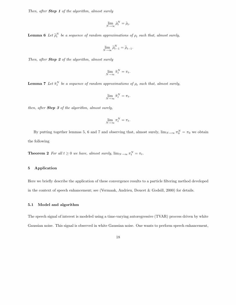
5.3 Experimental results
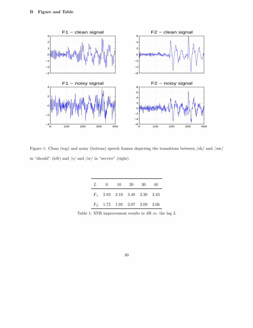
In Figure 1, we present two “clean” speech signals and their noisy versions corrupted artificially by some
white Gaussian noise. The Signal to Noise Ratios (SNR) are respectively equal to -0.61 decibels (dB) and
6.10dB.
Figure 1 about here.
We have applied the SMC method to these speech signals. In Table 1, we display the SNR improvement
in dB obtained using N = 500 particles when the point estimate chosen for the signal is
E (st| y1:t+L−1) =
∫stπt+L−1 (ds0:t+L−1, da0:t+L−1)
=
∫E (st| y1:t+L−1, a0:t+L−1)πt+L−1 (da0:t+L−1)
≃∫
E (st| y1:t+L−1, a0:t+L−1)πNt+L−1 (da0:t+L−1)
≃ 1
N
N∑
i=1
E(
st| y1:t+L−1, a(i)0:t+L−1
),
where L is the length of lag delay and E(
st| y1:t+L−1, a(i)0:t+L−1
)is computed through the Kalman filter.
Table 1 about here.
20

The SNR improvements results were obtained by averaging over 50 independent runs of the algorithms.
The fixed-lag estimates, i.e. L > 0, perform significantly better than the filtering estimates. The MCMC
step significantly improves the point estimate E (st| y1:t+L−1) by limiting the sample depletion problem.
One can listen to the results at http://www-svr.eng.cam.ac.uk/~jv211/audio/phd/index.html.
6 Discussion
We have given sufficient conditions to ensure convergence of a general SMC scheme. Essentially, one only
requires that the importance weights are bounded and that the selection scheme has a small discrepancy in
order to ensure convergence of the average mean square error. Further, if one assumes that the importance
kernel and the MCMC kernel are Feller continuous, that the importance weight function is continuous and
that the error introduced in the selection scheme is controlled by an inequality such as (14), then the resulting
approximating measure converges weakly to the posterior measure.
Of course, a natural question would be to ask which models and algorithms have uniform rates of
convergence (in time); that is for which the constant ct in Theorem 1 is independent of t. However, our
intention here was to present convergence results valid under very weak assumptions so as to include models
and algorithms used routinely by practitioners. Therefore, the set-up we chose to work with was too general
to allow for these more refined uniform convergence results. However, if one imposes appropriate additional
assumptions on the signal and on the observation process then such uniform rates are obtainable for the
class of methods we described above; see Del Moral & Guionnet (2001) for results of this kind. We will
address this issue in a subsequent paper.
7 Acknowledgments
We are thankful to Jaco Vermaak for providing us with most of the simulation results.
21

A Proofs of Lemmas and Theorems
Proof of Lemma 1. Let Gt−1 be the σ-field generated byx
(i)0:t−1
N
i=1, then
E[(
ρNt , ft
)∣∣∣Gt−1
]=
(πN
t−1, ΞπN
t−1
t ft
)
and
E
[((ρN
t , ft
)− E
[(ρN
t , ft
)∣∣∣Gt−1
])2∣∣∣∣Gt−1
]= E
[((ρN
t , ft
)−(
πNt−1, Ξ
πNt−1
t ft
))2∣∣∣∣∣Gt−1
]
=1
N
((πN
t−1, ΞπN
t−1
t f2t
)−(
πNt−1, Ξ
πNt−1
t ft
)2)
≤ ‖ft‖2N
.
From (10) we have that
∣∣∣∣(
πNt−1, Ξ
πNt−1
t ft
)−(πN
t−1, Ξπt−1
t ft
)∣∣∣∣ =
∣∣∣∣(
πNt−1, Ξ
πNt−1
t ft − Ξπt−1
t ft
)∣∣∣∣
≤∥∥∥∥Ξ
πNt−1
t ft − Ξπt−1
t ft
∥∥∥∥
≤ dt
∣∣(πNt−1, ft−1
)− (πt−1, ft−1)
∣∣ ,
hence,
E
[((πN
t−1, ΞπN
t−1
t ft
)−(πN
t−1, Ξπt−1
t ft
))2]≤ dtct−1
‖ft‖2N
.
Then, as Ξt , Ξπt−1
t ,
∣∣∣(ρN
t , ft
)− (ρt, ft)
∣∣∣ ≤∣∣∣∣(ρN
t , ft
)−(
πNt−1Ξ
πNt−1
t , ft
)∣∣∣∣+∣∣∣∣(
πNt−1Ξ
πNt−1
t , ft
)−(πN
t−1Ξt, ft
)∣∣∣∣
+∣∣(πN
t−1Ξt, ft
)− (πt−1Ξt, ft)
∣∣
and
E
[((ρN
t , ft
)−(πN
t−1, Ξtft
))2] 1
2
≤ E
[((ρN
t , ft
)−(Ξtπ
Nt−1, ft
))2] 1
2
22

+E
[((πN
t−1ΞπN
t−1
t , ft
)−(πN
t−1Ξt, ft
))2] 1
2
+E[((
πNt−1Ξt, ft
)− (πt−1Ξt, ft)
)2] 12
≤√
ct
‖ft‖√N
,
where ct =(1 +
√dtct−1 +
√ct−1
)2.
Proof of Lemma 2. We have using (11) and (12) that
∣∣∣∣∣∣∣∣
(ρN
t , ftgthπN
t−1
t
)
(ρN
t , gthπN
t−1
t
) −
(ρN
t , ftgthπN
t−1
t
)
(ρN
t , gtht
)
∣∣∣∣∣∣∣∣=
∣∣∣∣(
ρNt , ftgth
πNt−1
t
)∣∣∣∣∣∣∣∣(
ρNt , gt
(h
πNt−1
t − ht
))∣∣∣∣(ρN
t , gthπN
t−1
t
)(ρN
t , gtht
)
≤ ||ft||
∣∣∣∣(
ρNt , gt
(h
πNt−1
t − ht
))∣∣∣∣(ρN
t , gtht
)
≤ ||ft||∣∣∣∣(
ρNt , gt
(h
πNt−1
t − ht
))∣∣∣∣
∣∣∣∣∣∣1(
ρNt , gtht
) − 1
(ρt, gtht)
∣∣∣∣∣∣
+ ||ft||
∣∣∣∣(
ρNt , gt
(h
πNt−1
t − ht
))∣∣∣∣(ρt, gtht)
≤ ||ft|| et
(ρN
t , gtht
)∣∣∣(ρN
t , gtht
)− (ρt, gtht)
∣∣∣(ρN
t , gtht
)(ρt, gtht)
+ ||ft||∣∣(πN
t−1, fh)−(πt−1, f
h)∣∣
(ρt, gtht)
≤ ||ft||(ρt, gtht)
(et
∣∣∣(ρN
t , gtht
)− (ρt, gtht)
∣∣∣
+∣∣(πN
t−1, fh)−(πt−1, f
h)∣∣) .
Hence,
E
(ρN
t , ftgthπN
t−1
t
)
(ρN
t , gthπN
t−1
t
) −
(ρN
t , ftgthπN
t−1
t
)
(ρN
t , gtht
)
2
12
≤ ||ft||(et
√ct ||gtht||+√ct−1
∣∣∣∣fh∣∣∣∣)
(ρt, gtht)√
N. (18)
23

We have, using (12),
∣∣∣∣∣∣∣
1(ρN
t , gthπN
t−1
t
) − 1(ρN
t , gtht
)
∣∣∣∣∣∣∣=
∣∣∣∣(
ρNt , gt
(h
πNt−1
t − ht
))∣∣∣∣(ρN
t , gthπN
t−1
t
)(ρN
t , gtht
)
≤et
(ρN
t , gtht
)
(ρN
t , gthπN
t−1
t
)(ρN
t , gtht
)
=et(
ρNt , gth
πNt−1
t
) ,
so∣∣∣∣∣∣∣∣
(ρN
t , ftgthπN
t−1
t
)
(ρN
t , gtht
) −
(ρN
t , ftgthπN
t−1
t
)
(ρt, gtht)
∣∣∣∣∣∣∣∣=
∣∣∣(ρN
t , gtht
)− (ρt, gtht)
∣∣∣(ρt, gtht)
∣∣∣∣(
ρNt , ftgth
πNt−1
t
)∣∣∣∣(ρN
t , gtht
)
≤
∣∣∣(ρN
t , gtht
)− (ρt, gtht)
∣∣∣(ρt, gtht)
∣∣∣∣(
ρNt , ftgth
πNt−1
t
)∣∣∣∣
×
∣∣∣∣∣∣∣
1(ρN
t , gtht
) − 1(ρN
t , gthπN
t−1
t
)
∣∣∣∣∣∣∣
+
∣∣∣(ρN
t , gtht
)− (ρt, gtht)
∣∣∣(ρN
t , gthπN
t−1
t
)(ρt, gtht)
∣∣∣∣(
ρNt , ftgth
πNt−1
t
)∣∣∣∣
≤
∣∣∣(ρN
t , gtht
)− (ρt, gtht)
∣∣∣(ρt, gtht)
∣∣∣∣(
ρNt , ftgth
πNt−1
t
)∣∣∣∣et(
ρNt , gth
πNt−1
t
)
+
∣∣∣(ρN
t , gtht
)− (ρt, gtht)
∣∣∣(ρN
t , gthπN
t−1
t
)(ρt, gtht)
∣∣∣∣(
ρNt , ftgth
πNt−1
t
)∣∣∣∣
≤ (et + 1) ||ft||
∣∣∣(ρN
t , gtht
)− (ρt, gtht)
∣∣∣(ρt, gtht)
and∣∣∣∣∣∣∣∣
(ρN
t , ftgthπN
t−1
t
)
(ρt, gtht)−
(ρN
t , ftgtht
)
(ρt, gtht)
∣∣∣∣∣∣∣∣≤
(ρN
t , |ft|∣∣∣∣gth
πNt−1
t − gtht
∣∣∣∣)
(ρt, gtht)≤ ||ft||
∣∣(πNt−1, f
h)−(πt−1, f
h)∣∣
(ρt, gtht)
∣∣∣∣∣∣
(ρN
t , ftgtht
)
(ρt, gtht)− (ρt, ftgtht)
(ρt, gtht)
∣∣∣∣∣∣≤
∣∣∣(ρN
t , ftgtht
)− (ρt, ftgtht)
∣∣∣(ρt, gtht)
.
24

Hence,
E
(ρN
t , ftgthπN
t−1
t
)
(ρN
t , gtht
) − (ρt, ftgtht)
(ρt, gtht)
2
12
≤ ||ft||((et + 2)
√ct ||gtht||+√ct−1
∣∣∣∣fh∣∣∣∣)
(ρt, gtht)√
N. (19)
From (18) and (19), the result follows with
ct =
(2 (et + 1)
√ct ||gtht||+ 2
√ct−1
∣∣∣∣fh∣∣∣∣)2
(ρt, gtht)2 .
Proof of Lemma 3. Since
∣∣(πNt , ft
)− (πt, ft)
∣∣ ≤∣∣(πN
t , ft
)−(πN
t , ft
)∣∣+∣∣(πN
t , ft
)− (πt, ft)
∣∣ ,
we get from lemma 2 and (13) that
E[((
πNt , ft
)− (πt, ft)
)2] 12 ≤ E
[((πN
t , ft
)−(πN
t , ft
))2] 12
+ E[((
πNt , ft
)− (πt, ft)
)2] 12
≤√
ct
‖ft‖2√N
,
where√
ct =√
Ct +√
ct.
Proof of Lemma 4. Let Ht be the σ-field generated by
x(i)0:t
N
i=1, then
E[(
πNt , ft
)∣∣Ht
]=(πN
t , Ktft
)
and one has
E[((
πNt , ft
)− E
[(πN
t , ft
)∣∣Ht
])2∣∣∣Ht
]=
1
N
((πN
t , Ktf2t
)−(πN
t , Ktft
)2)
≤ 1
N
(πN
t , Ktf2t
)≤ ‖ft‖2
N,
thus,
E[((
πNt , ft
)− (πt, ft)
)2] 12 ≤ E
[((πN
t , ft
)−(πN
t , Ktft
))2] 12
+ E[((
πNt , Ktft
)− (πt, Ktft)
)2] 12
≤ √ct
‖ft‖√N
,
25
where ct =(√
ct + 1)2
.
Remark 2 It is actually possible to consider a global Markov transition kernel on the N -fold space admitting
the N -fold posterior distribution as invariant distribution, that is,
∫Kt
(x
(i)0:t
N
i=1, dx
(i)0:t
N
i=1
) N∏
i=1
πt
(dx
(i)0:t
)=
N∏
i=1
πt
(dx
(i)0:t
).
Let us introduce the following notation: for any set of indices i1, . . . , in (i1 6= i2 6= . . . 6= in)
Ki1,...,in
t
(x
(i)0:t
N
i=1, d(x
(i1)0:t , . . . , dx
(in)0:t
)) , ∫ Kt
(x
(i)0:t
N
i=1, dx
(i)0:t
N
i=1
),
where the integration is overx
(i)0:t; i ∈ 1, . . . , N \ i1, . . . , in
. If we restrict ourselves to the case where
the kernels Kit
(x
(i)0:t
N
i=1, dx0:t
)are equal for all i = 1, . . . , N , convergence is still ensured under the
following “mixing” assumption on the MCMC kernel: for any ft ∈ B((Rnx )
t+1)
∑
i6=j
∣∣∣∣∣
∫Ki,j
t
(x
(i)0:t
N
i=1, d(x
(i)0:t, x
(j)0:t
))ft
(x
(i)0:t
)ft
(x
(j)0:t
)−(∫
Kt
(x
(i)0:t
N
i=1, dx0:t
)ft (x0:t)
)2∣∣∣∣∣ < Mt
‖ft‖2N
.
(20)
Proof of Theorem 1. At time t = 0, we have assumed to sample N i.i.d. particles from π0, so
E[((
πN0 , f0
)− (π0, f0)
)2] ≤ ‖f0‖2N
and the result follows straightforwardly from Lemmas 1, 2, 3 and 4.
Proof of Lemma 5. Let Gt−1 be the σ-field generated byx
(i)0:t−1
N
i=1, then
E[(
ρNt , ft
)|Gt−1
]=
(πN
t−1, ΞπN
t−1
t ft
). (21)
Since, conditionally on Gt−1,x
(i)0:t
N
i=1are i.i.d. random variables, there exists a constant C independent of
N such that
E[((
ρNt , ft
)− E
[(ρN
t , ft
)|Gt−1
])4 |Gt−1
]≤ C ||ft||4
N2. (22)
26
From (21) and (22), we get that
E
[((ρN
t , ft
)−(
πNt−1, Ξ
πNt−1
t ft
))4]≤ C ||ft||4
N2,
hence, via a Borel-Cantelli argument, we have, almost surely,
limN→∞
(ρN
t , ft
)−(
πNt−1, Ξ
πNt−1
t ft
)= 0. (23)
Now∥∥∥∥(
πNt−1,
(Ξ
πNt−1
t − Ξt
)ft
)∥∥∥∥ ≤ dt
∣∣(πNt−1, ft
)− (πt−1, ft)
∣∣
so almost surely
limN→∞
(ρN
t , ft
)−(πN
t−1, Ξtft
)= 0.
But since Ξtft is a continuous function (using the Feller property of Ξt) and, almost surely, limN→∞ πNt−1 =
πt−1, then, from (23), one has
limN→∞
(ρN
t , ft
)= (πt−1, Ξtft) = (ρt, ft) .
Proof of Lemma 6. From the definition of πNt we have that for any ft ∈ B
((Rnx )
t+1)
(πN
t , f)
=
(ρN
t , ftgtht
)(ρN
t , gtht
) .
Since, almost surely, limN→∞ ρNt = ρt, we have that
(ρN
t , ftgthπN
t−1
t
)as by assumption gth
πNt−1
t is a bounded
continuous function
limN→∞
(ρN
t , ftgthπN
t−1
t
)=
(ρt, ftgth
πNt−1
t
)limN→∞
(ρN
t , gthπN
t−1
t
)=
(ρt, gth
πNt−1
t
)
and
∥∥∥∥(
ρt, ftgthπN
t−1
t
)− (ρt, ftgtht)
∥∥∥∥ ≤ ‖ft‖∣∣(πN
t−1, fh)−(πt−1, f
h)∣∣
∥∥∥∥(
ρt, gthπN
t−1
t
)− (ρt, gtht)
∥∥∥∥ ≤∣∣(πN
t−1, fh)−(πt−1, f
h)∣∣ ,
27
so since, almost surely, limN→∞ πNt−1 = πt−1 then
limN→∞
(ρN
t , ftgtht
)= (ρt, ftgtht) , limN→∞
(ρN
t , gtht
)= (ρt, gtht)
as by assumption gtht is a bounded continuous function. Hence, almost surely, limN→∞
(πN
t , ft
)= (eρt,ftgtht)
(ρt,gtht)=
(πt, ft) for any ft ∈ B((Rnx )
t+1)
and, therefore, limN→∞ πNt = πt. Now, from (14), we have
E[∣∣(πN
t , ft
)−(πN
t , ft
)∣∣p]≤ Ct ||ft||p
N1+ε, (24)
where ε = p− α− 1 > 0. From (24) again via a Borel-Cantelli argument, we have, almost surely, that
limN→∞
(πN
t , ft
)−(πN
t , ft
)= 0,
hence the claim.
Proof of Lemma 7. The proof is identical to that of lemma 5. Let Ht be the σ-field generated by
x
(i)0:t
N
i=1, then
E[(
πNt , f
)|Ht
]=(πN
t , Ktf). (25)
Also it is relatively easy to prove that there exists a constant C independent of N such that
E[((
πNt , f
)− E
[(πN
t , f)|Ht
])4 |Ht
]≤ C ||f ||4
N2. (26)
From (25) and (26), we get that
E[((
πNt , f
)−(πN
t , Ktf))4] ≤ Ct ||f ||4
N2
hence, via a Borel-Cantelli argument, we have, almost surely,
limN→∞
(πN
t , f)−(πN
t , Ktf)
= 0. (27)
But since Ktf is a continuous function (using the Feller property of Kt) and, almost surely, limN→∞ πNt−1 =
πt−1, we have, from (27), that
limN→∞
(πN
t , f)
= (πt, Ktf) = (πtKt, f) = (πt, f) .
28

which gives our claim.
Proof of Theorem 2. By putting together lemmas 5, 6 and 7 and observing that, almost surely, limN→∞ πN0 =
π0 we straightforwardly obtain the result.
29
B Figure and Table
−3
−2
−1
0
1
2
3F1 − clean signal
0 100 200 300 400−4
−2
0
2
4F1 − noisy signal
−6
−4
−2
0
2
4
6F2 − clean signal
0 100 200 300 400−6
−4
−2
0
2
4
6
8F2 − noisy signal
Figure 1: Clean (top) and noisy (bottom) speech frames depicting the transitions between /sh/ and /uw/
in “should” (left) and /s/ and /er/ in “service” (right).
L 0 10 20 30 40
F1 2.83 3.10 3.40 3.30 3.43
F2 1.72 1.92 2.07 2.09 2.06
Table 1: SNR improvement results in dB vs. the lag L
30

References
Berzuini C., Best N., Gilks W.R. & Larizza C. (1997) Dynamic conditional independence models and
Markov chain Monte Carlo methods. J. Am. Statist. Ass., 92, 1403-1412.
Carpenter J., Clifford P. & Fearnhead P. (1999) Building robust simulation-based filters for evolving
data sets. Technical report, University of Oxford, Dept. of Statistics.
Chen R. & Liu J.S. (2000) Mixture Kalman filters. J. R. Statist. Soc. B, 62, 493-508.
Crisan D., Del Moral P. & Lyons T. (1999) Discrete filtering using branching and interacting particle
systems. Markov Proc. Rel. Fields, 5, 293-318.
Crisan D. (2001) Particle filters - A theoretical perspective. In Sequential Monte Carlo Methods in
Practice (eds A. Doucet, J.F.G. de Freitas & N.J. Gordon). New-York: Springer-Verlag.
Del Moral P. (1996) Non linear filtering: interacting particle solution. Markov Proc. Rel. Fields, 2,
555-580.
Del Moral P. (1997) Measure valued processes and interacting particle systems. Application to non
linear filtering problems. Ann. Appl. Proba., 8, 438-495.
Del Moral P. & Guionnet A. (2001) On the stability of interacting processes with applications to
filtering and genetic algorithms. Ann. Instit. Henri Poincare. to appear.
Doucet A., de Freitas J.F.G. & Gordon N.J. (eds.) (2001) Sequential Monte Carlo Methods in Practice.
New York: Springer-Verlag.
Doucet A., Godsill S.J. & Andrieu C. (2000) On sequential Monte Carlo sampling methods for Bayesian
filtering. Statist. Comput., 10, 197-208.
31
Fox D., Thrun S., Burgard W. & Dellaert F. (2001). Particle filters for mobile robot localization. In
Sequential Monte Carlo Methods in Practice (eds A. Doucet, J.F.G. de Freitas and N.J. Gordon). New
York: Springer-Verlag.
Gilks W.R. & Berzuini C. (1999) Following a moving target - Monte Carlo inference for dynamic
Bayesian models. submitted to J. R. Statist. Soc. B.
Gordon N.J., Salmond D.J. & Smith A.F.M. (1993) Novel approach to nonlinear/non-Gaussian
Bayesian state estimation. IEE Proc. F, 140, 107-113.
Higuchi T. (1997) Monte Carlo filter using the genetic algorithm operators. J. Statist. Comput. Simul.,
59, 1-23.
Kitagawa G. (1996) Monte Carlo filter and smoother for non-Gaussian nonlinear state space models.
J. Comput. Graph. Statist., 5, 1-25.
Hurzeler M. & Kunsch, H.R. (1998) Monte Carlo approximations for general state space models. J.
Comput. Graph. Statist., 7, 175-193.
Iba Y. (2000) Population-based Monte Carlo algorithms. Research memorandum no. 757, Institute of
Statistical Mathematics, Tokyo.
Isard M. & Blake A. (1998) CONDENSATION – conditional density propagation for visual tracking,
Int. J. Computer Vision, 29, 5–28.
Liu J.S. & Chen R. (1998) Sequential Monte Carlo methods for dynamic systems. J. Am. Statist. Ass.,
93, 1032-1044.
Liu J. and West M. (2001) Combined parameter and state estimation in simulation-based filtering. In
Sequential Monte Carlo Methods in Practice (eds A. Doucet, J.F.G. de Freitas and N.J. Gordon). New
York: Springer-Verlag.
32

Pitt M.K. & Shephard N. (1999) Filtering via simulation: auxiliary particle filter. J. Am. Statist. Ass.,
94, 590-599.
Ripley B.D. (1987) Stochastic Simulation, New York: Wiley.
Robert C.P. & Casella G. (1999) Monte Carlo Statistical Methods. New York: Springer-Verlag.
Tanizaki H. (1996) Nonlinear Filters: Estimation and Applications. 2nd edition, Berlin: Springer-
Verlag.
Vermaak J., Andrieu C., Doucet A. & Godsill S.J. (2000) On-line Bayesian modelling and enhancement
of speech signals. Technical report CUED/F-INFENG/TR.361, Cambridge University.
West M. (1993a) Approximating posterior distributions by mixtures. J. R. Statist. Soc. B, 55, 409-422.
West M. (1993b) Mixture models, Monte Carlo, Bayesian updating and dynamic models. Comput.
Science Statist., 24, 325-333.
West M. & Harrison P.J. (1997) Bayesian Forecasting and Dynamic Models. 2nd edition, New York:
Springer-Verlag.
33