Sequence manipulation and scanning

Benjamin Jean-Marie Tremblay∗

17 October 2021

AbstractSequences stored as XStringSet objects (from the Biostrings package) can be used by several functions

in the universalmotif package. These functions are demonstrated here and fall into two categories: sequencemanipulation and motif scanning. Sequences can be generated, shuffled, and background frequenciesof any order calculated. Scanning can be done simply to find locations of motif hits above a certainthreshold, or to find instances of enriched motifs.

Contents1 Introduction 1

2 Basic sequence handling 22.1 Creating random sequences . . . . . . . . . . . . . . . . . . . . . . . . . . . . . . . . . . . . . 22.2 Calculating sequence background . . . . . . . . . . . . . . . . . . . . . . . . . . . . . . . . . . 32.3 Clustering sequences by k-let composition . . . . . . . . . . . . . . . . . . . . . . . . . . . . . 4

3 Shuffling 53.1 Shuffling sequences . . . . . . . . . . . . . . . . . . . . . . . . . . . . . . . . . . . . . . . . . . 53.2 Local shuffling . . . . . . . . . . . . . . . . . . . . . . . . . . . . . . . . . . . . . . . . . . . . 7

4 Sequence scanning and enrichment 84.1 Choosing a logodds threshold . . . . . . . . . . . . . . . . . . . . . . . . . . . . . . . . . . . . 84.2 Regular and higher order scanning . . . . . . . . . . . . . . . . . . . . . . . . . . . . . . . . . 124.3 Visualizing motif hits across sequences . . . . . . . . . . . . . . . . . . . . . . . . . . . . . . . 164.4 Enrichment analyses . . . . . . . . . . . . . . . . . . . . . . . . . . . . . . . . . . . . . . . . . 194.5 Fixed and variable-length gapped motifs . . . . . . . . . . . . . . . . . . . . . . . . . . . . . . 204.6 Detecting low complexity regions and sequence masking . . . . . . . . . . . . . . . . . . . . . 21

5 Motif discovery with MEME 23

6 Miscellaneous string utilities 25

Session info 26

References 28

1 IntroductionThis vignette goes through generating your own sequences from a specified background model, shufflingsequences whilst maintaining a certain k-let size, and the scanning of sequences and scoring of motifs. For anintroduction to sequence motifs, see the introductory vignette. For a basic overview of available motif-related

∗benjamin.tremblay@uwaterloo.ca

1

functions, see the motif manipulation vignette. For a discussion on motif comparisons and P-values, see themotif comparisons and P-values vignette.

2 Basic sequence handling2.1 Creating random sequencesThe Biostrings package offers an excellent suite of functions for dealing with biological sequences.The universalmotif package hopes to help extend these by providing the create_sequences() andshuffle_sequences() functions. The first of these, create_sequences(), generates a set of letters inrandom order, then passes these strings to the Biostrings package to generate the final XStringSet object.The number and length of sequences can be specified. The probabilities of individual letters can also be set.

The freqs option of create_sequences() also takes higher order backgrounds. In these cases the sequencesare constructed in a Markov-style manner, where the probability of each letter is based on which lettersprecede it.library(universalmotif)library(Biostrings)

## Create some DNA sequences for use with an external program (default## is DNA):

sequences.dna <- create_sequences(seqnum = 500,freqs = c(A=0.3, C=0.2, G=0.2, T=0.3))

## writeXStringSet(sequences.dna, "dna.fasta")sequences.dna#> DNAStringSet object of length 500:#> width seq#> [1] 100 GTTGACGAACTAAAATGAGTATATTTGTACGTA...CGTTAAGTGACGGAATACTCCCCGTATTATGA#> [2] 100 ATTGCTTATTGTTGCAGCAGGTGTGACTTTCTA...CTGATTTAATTTTGGCCGTTTGATGTCCCACT#> [3] 100 AACACGCTACCGTCATGAATACGCCAATGCAAT...AAAAATTACCACATACGATGATTGAGCTATGC#> [4] 100 GGTTCCGACTAGACTAAGATTAAGATTTGCACC...ACTGTTGTAAATTATATAATTCTAGCCGCTTT#> [5] 100 GTTCAACATGAATCGTAGAATGACAATGTGTTT...CCTTACAGAAGCTTGTAGTGGCTGACCCATAG#> ... ... ...#> [496] 100 AGAACGCCGCTTCTTGCTTAAGGACGTGTGCGC...GGAAGGTATTGAACTTGATGTCGTATAACAAA#> [497] 100 GACGGAAAAAAACCGGTGCGCGAATAACTATCG...TCGCGAAAAAACTTAACTGGCTACTAACCTAG#> [498] 100 TAGCGCGAGTGCGGACGATTGCTATAAATTAAT...TTCATTGAGAGTAGACAGGATACAGTTAATGT#> [499] 100 TGCAATGAGGCATAGTATTCGTCGTCTAAAATG...GTTCCATTTCCGTCAAAGAGTTCTGATCCTCC#> [500] 100 CTATAGTTGACTCCTGGTATACCTCCCACAGTA...TTCATTTAAACTGATAACAGCGTACAGTCCGT

## Amino acid:

create_sequences(alphabet = "AA")#> AAStringSet object of length 100:#> width seq#> [1] 100 DPHAWVCCSHTLPYKINRVIKGMKCFLALRKRQ...SAYLCRAWQANYFQNMYCHCCGLFSQPNAGCN#> [2] 100 HPNFNNYHNGFCVNQFKFSIMYKTFANDHTLSL...VTCIRCLQPYRCMVARCGAWVMYLYHAHSYYG#> [3] 100 ETPNIYLPDSGESCDRHAPMKIDYPYWRMDNQH...GPWHTVQPAAADAENHPLFNTMHEGDTIPLRV#> [4] 100 IRLEKWNSWSDYKNKPRAYAMMKIYPDFTHAPE...AKCRAHEDWDWFNNEALGCYLHEPSDDLWCHK#> [5] 100 FTTLCWFGMNFPVRTNWQQWHFELVSCIFTAQN...YNNERIDHHAVLHVLHIVCEHPITTKVRIDMN#> ... ... ...#> [96] 100 VMDCWTAKTPGNLMIHVDLYHCCDLPPVKITIG...AAADQGPMQCYPEMYILQRCYVHCIEDKFFPR#> [97] 100 QPPGCCEMLWTYGTWEQHDNFVKCWFDKPPRFS...VSCQCMWLDFTHPVRGFLNGLAYNVLLYVIWA#> [98] 100 SWTWSRRSPRTEPWRKMKFANPAWVDRVTFCEI...CYFKTEHRLSYWQCTWDMMWVGWLWGRHGFCV

2

#> [99] 100 TYKEAECADMYWRTLGDLRKFYKFKEYLWFSDI...ACYNNYCMVPHINEIARYLHWYRLVDHEELDI#> [100] 100 CWRHFVNLYLKDHVPGPKYCPCVRRHCMGYQMT...WTLGNHRPEGWFCPVNTLMAMKYKCFVGVSAW

## Any set of characters can be used

create_sequences(alphabet = paste0(letters, collapse = ""))#> BStringSet object of length 100:#> width seq#> [1] 100 hmjatxotqqapcpusecxfvbpnobwehatjw...ckfzixtwjmdgtvoveuxjawzxufffpcox#> [2] 100 knreotsdvkkcohjeeaqswyncgtgdbpznl...jsotyklqoilkfbmqzlxizmhhcbtkjicm#> [3] 100 ozxmldaerchrbgxdwrymijbzazjolycdp...fmegpientlmxgisdxjffcphsmlqzrchy#> [4] 100 rfwiucnyuuckdrtasekcidxdeplurorre...ffwovgarqnekuomacvmkhcmcumzxejqm#> [5] 100 fpenqswakeieeooxhszfpkvbefkmkbrow...lxxehzvtphernpbrmmuavolcngsqcrlp#> ... ... ...#> [96] 100 vkytzcjzauwrjouapamcshuoodgzwakih...lwvvxqxzylvvfuihwbwcawjmpvaiqclh#> [97] 100 asfaodjykqlnsnxpmglxbihbpzymvwjpc...ieeyjcfoqklrlszoefugqhvuyhjyrrci#> [98] 100 xgnmjeyvpccrqulsuwljzcewzotqeovjb...ilejnrfuromqphmxahwigxiiipazubsk#> [99] 100 jcstyqrbcttpnrtsglbwmlhqjsxdgociv...hjvriozotfwoxmgwfujmkwyxsbbczexx#> [100] 100 jsbilbmwimwwidlgufjdhusrqajnppnga...harzhuhwqnbxryuirjnyoewbcmbkzesg

2.2 Calculating sequence backgroundSequence backgrounds can be retrieved for DNA and RNA sequences with oligonucleotideFrequency()from "Biostrings. Unfortunately, no such Biostrings function exists for other sequence alphabets. Theuniversalmotif package proves get_bkg() to remedy this. Similarly, the get_bkg() function can calculatehigher order backgrounds for any alphabet as well. It is recommended to use the original Biostrings forvery long (e.g. billions of characters) DNA and RNA sequences whenever possible though, as it is much fasterthan get_bkg().library(universalmotif)

## Background of DNA sequences:dna <- create_sequences()get_bkg(dna, k = 1:2)#> DataFrame with 20 rows and 3 columns#> klet count probability#> <character> <numeric> <numeric>#> 1 A 2398 0.2398000#> 2 C 2479 0.2479000#> 3 G 2537 0.2537000#> 4 T 2586 0.2586000#> 5 AA 573 0.0578788#> ... ... ... ...#> 16 GT 626 0.0632323#> 17 TA 608 0.0614141#> 18 TC 635 0.0641414#> 19 TG 667 0.0673737#> 20 TT 650 0.0656566

## Background of non DNA/RNA sequences:qwerty <- create_sequences("QWERTY")get_bkg(qwerty, k = 1:2)#> DataFrame with 42 rows and 3 columns#> klet count probability

3

#> <character> <numeric> <numeric>#> 1 E 1613 0.1613#> 2 Q 1708 0.1708#> 3 R 1664 0.1664#> 4 T 1608 0.1608#> 5 W 1691 0.1691#> ... ... ... ...#> 38 YQ 297 0.0300000#> 39 YR 278 0.0280808#> 40 YT 265 0.0267677#> 41 YW 313 0.0316162#> 42 YY 266 0.0268687

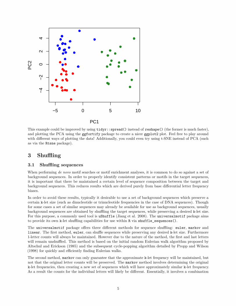
2.3 Clustering sequences by k-let compositionOne way to compare sequences is by k-let composition. The following example illustrates how one could goabout doing this using only the universalmotif package and base graphics.library(universalmotif)

## Generate three random sets of sequences:s1 <- create_sequences(seqnum = 20,

freqs = c(A = 0.3, C = 0.2, G = 0.2, T = 0.3))s2 <- create_sequences(seqnum = 20,

freqs = c(A = 0.4, C = 0.4, G = 0.1, T = 0.1))s3 <- create_sequences(seqnum = 20,

freqs = c(A = 0.2, C = 0.3, G = 0.3, T = 0.2))

## Create a function to get properly formatted k-let counts:get_klet_matrix <- function(seqs, k, groupName) {

bkg <- get_bkg(seqs, k = k, merge.res = FALSE)bkg <- bkg[, c("sequence", "klet", "count")]bkg <- reshape(bkg, idvar = "sequence", timevar = "klet",

direction = "wide")as.data.frame(cbind(Group = groupName, bkg))

}

## Calculate k-let content (up to you what size k you want!):s1 <- get_klet_matrix(s1, 4, 1)s2 <- get_klet_matrix(s2, 4, 2)s3 <- get_klet_matrix(s3, 4, 3)

# Combine everything into a single object:sAll <- rbind(s1, s2, s3)

## Do the PCA:sPCA <- prcomp(sAll[, -(1:2)])

## Plot the PCA:plot(sPCA$x, col = c("red", "forestgreen", "blue")[sAll$Group], pch = 19)

4

−5 0 5 10

−4

−2

02

4

PC1

PC

2

This example could be improved by using tidyr::spread() instead of reshape() (the former is much faster),and plotting the PCA using the ggfortify package to create a nicer ggplot2 plot. Feel free to play aroundwith different ways of plotting the data! Additionally, you could even try using t-SNE instead of PCA (suchas via the Rtsne package).

3 Shuffling3.1 Shuffling sequencesWhen performing de novo motif searches or motif enrichment analyses, it is common to do so against a set ofbackground sequences. In order to properly identify consistent patterns or motifs in the target sequences,it is important that there be maintained a certain level of sequence composition between the target andbackground sequences. This reduces results which are derived purely from base differential letter frequencybiases.

In order to avoid these results, typically it desirable to use a set of background sequences which preserve acertain k-let size (such as dinucleotide or trinucleotide frequencies in the case of DNA sequences). Thoughfor some cases a set of similar sequences may already be available for use as background sequences, usuallybackground sequences are obtained by shuffling the target sequences, while preserving a desired k-let size.For this purpose, a commonly used tool is uShuffle (Jiang et al. 2008). The universalmotif package aimsto provide its own k-let shuffling capabilities for use within R via shuffle_sequences().

The universalmotif package offers three different methods for sequence shuffling: euler, markov andlinear. The first method, euler, can shuffle sequences while preserving any desired k-let size. Furthermore1-letter counts will always be maintained. However due to the nature of the method, the first and last letterswill remain unshuffled. This method is based on the initial random Eulerian walk algorithm proposed byAltschul and Erickson (1985) and the subsequent cycle-popping algorithm detailed by Propp and Wilson(1998) for quickly and efficiently finding Eulerian walks.

The second method, markov can only guarantee that the approximate k-let frequency will be maintained, butnot that the original letter counts will be preserved. The markov method involves determining the originalk-let frequencies, then creating a new set of sequences which will have approximately similar k-let frequency.As a result the counts for the individual letters will likely be different. Essentially, it involves a combination

5

of determining k-let frequencies followed by create_sequences(). This type of pseudo-shuffling is discussedby Fitch (1983).

The third method linear preserves the original 1-letter counts exactly, but uses a more crude shufflingtechnique. In this case the sequence is split into sub-sequences every k-let (of any size), which are thenre-assembled randomly. This means that while shuffling the same sequence multiple times with method= "linear" will result in different sequences, they will all have started from the same set of k-lengthsub-sequences (just re-assembled differently).library(universalmotif)library(Biostrings)data(ArabidopsisPromoters)

## Potentially starting off with some external sequences:# ArabidopsisPromoters <- readDNAStringSet("ArabidopsisPromoters.fasta")

euler <- shuffle_sequences(ArabidopsisPromoters, k = 2, method = "euler")markov <- shuffle_sequences(ArabidopsisPromoters, k = 2, method = "markov")linear <- shuffle_sequences(ArabidopsisPromoters, k = 2, method = "linear")k1 <- shuffle_sequences(ArabidopsisPromoters, k = 1)

Let us compare how the methods perform:o.letter <- get_bkg(ArabidopsisPromoters, 1)e.letter <- get_bkg(euler, 1)m.letter <- get_bkg(markov, 1)l.letter <- get_bkg(linear, 1)

data.frame(original=o.letter$count, euler=e.letter$count,markov=m.letter$count, linear=l.letter$count, row.names = DNA_BASES)

#> original euler markov linear#> A 17384 17384 17520 17384#> C 8081 8081 8045 8081#> G 7583 7583 7447 7583#> T 16952 16952 16988 16952

o.counts <- get_bkg(ArabidopsisPromoters, 2)e.counts <- get_bkg(euler, 2)m.counts <- get_bkg(markov, 2)l.counts <- get_bkg(linear, 2)

data.frame(original=o.counts$count, euler=e.counts$count,markov=m.counts$count, linear=l.counts$count,row.names = get_klets(DNA_BASES, 2))

#> original euler markov linear#> AA 6893 6893 6140 6456#> AC 2614 2614 2827 2705#> AG 2592 2592 2576 2601#> AT 5276 5276 5961 5601#> CA 3014 3014 2811 2930#> CC 1376 1376 1312 1344#> CG 1051 1051 1192 1149#> CT 2621 2621 2720 2651#> GA 2734 2734 2621 2692#> GC 1104 1104 1209 1169#> GG 1176 1176 1171 1160

6

#> GT 2561 2561 2443 2557#> TA 4725 4725 5929 5285#> TC 2977 2977 2689 2858#> TG 2759 2759 2501 2669#> TT 6477 6477 5848 6123

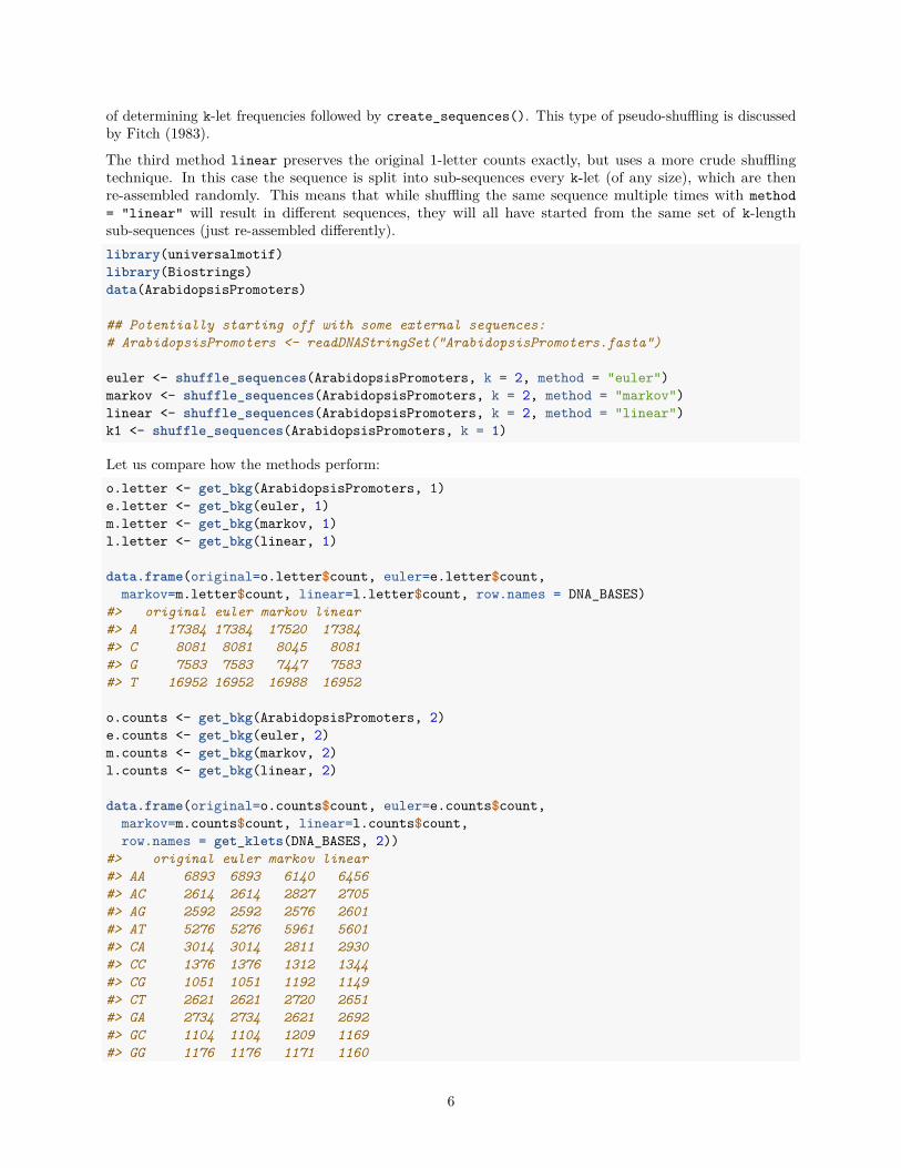
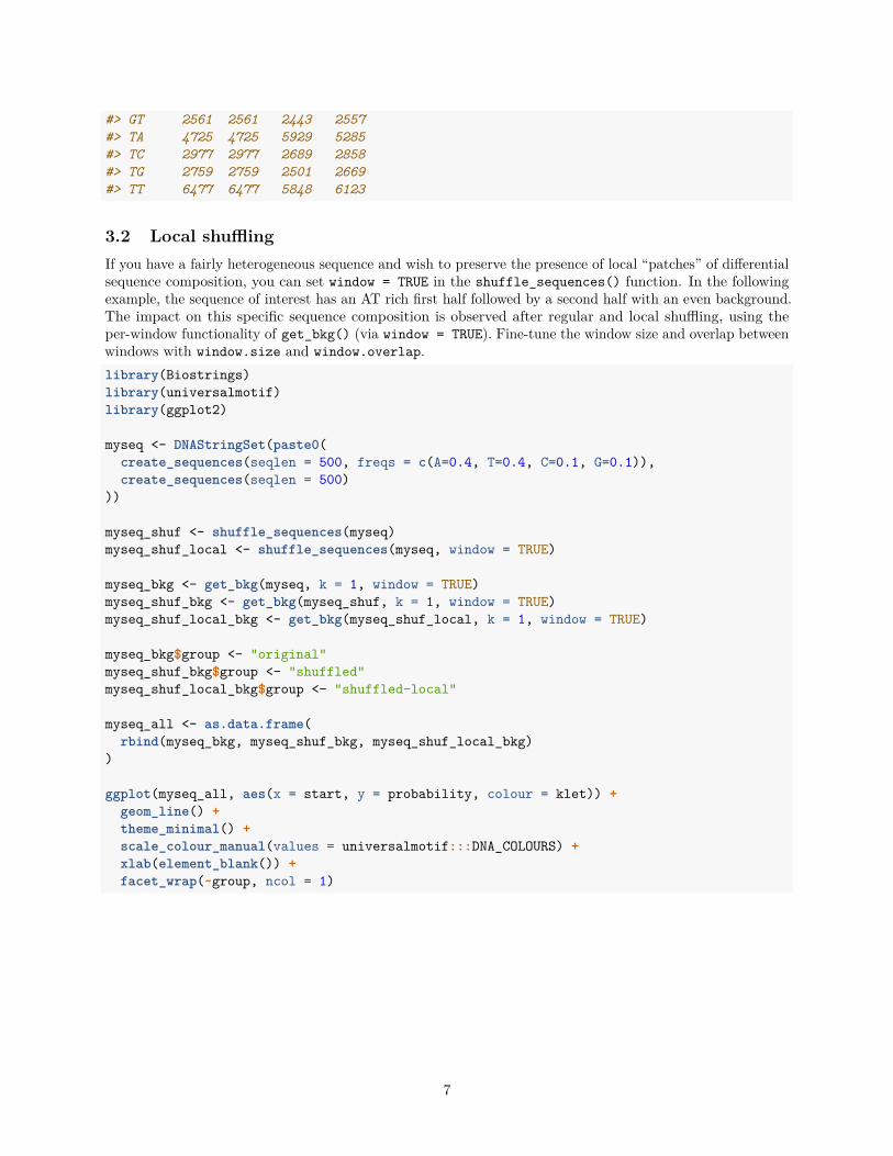
3.2 Local shufflingIf you have a fairly heterogeneous sequence and wish to preserve the presence of local “patches” of differentialsequence composition, you can set window = TRUE in the shuffle_sequences() function. In the followingexample, the sequence of interest has an AT rich first half followed by a second half with an even background.The impact on this specific sequence composition is observed after regular and local shuffling, using theper-window functionality of get_bkg() (via window = TRUE). Fine-tune the window size and overlap betweenwindows with window.size and window.overlap.library(Biostrings)library(universalmotif)library(ggplot2)

myseq <- DNAStringSet(paste0(create_sequences(seqlen = 500, freqs = c(A=0.4, T=0.4, C=0.1, G=0.1)),create_sequences(seqlen = 500)

))

myseq_shuf <- shuffle_sequences(myseq)myseq_shuf_local <- shuffle_sequences(myseq, window = TRUE)

myseq_bkg <- get_bkg(myseq, k = 1, window = TRUE)myseq_shuf_bkg <- get_bkg(myseq_shuf, k = 1, window = TRUE)myseq_shuf_local_bkg <- get_bkg(myseq_shuf_local, k = 1, window = TRUE)

myseq_bkg$group <- "original"myseq_shuf_bkg$group <- "shuffled"myseq_shuf_local_bkg$group <- "shuffled-local"

myseq_all <- as.data.frame(rbind(myseq_bkg, myseq_shuf_bkg, myseq_shuf_local_bkg)

)

ggplot(myseq_all, aes(x = start, y = probability, colour = klet)) +geom_line() +theme_minimal() +scale_colour_manual(values = universalmotif:::DNA_COLOURS) +xlab(element_blank()) +facet_wrap(~group, ncol = 1)

7

shuffled−local

shuffled

original

0 250 500 750

0.1

0.2

0.3

0.4

0.1

0.2

0.3

0.4

0.1

0.2

0.3

0.4

prob

abili

ty

klet

A

C

G

T

4 Sequence scanning and enrichmentThere are many motif-programs available with sequence scanning capabilities, such as HOMER and toolsfrom the MEME suite. The universalmotif package does not aim to supplant these, but rather provideconvenience functions for quickly scanning a few sequences without needing to leave the R environment.Furthermore, these functions allow for taking advantage of the higher-order (multifreq) motif formatdescribed here.

Two scanning-related functions are provided: scan_sequences() and enrich_motifs(). The latter simplyruns scan_sequences() twice on a set of target and background sequences. Given a motif of length n,scan_sequences() considers every possible n-length subset in a sequence and scores it using the PWMformat. If the match surpasses the minimum threshold, it is reported. This is case regardless of whether oneis scanning with a regular motif, or using the higher-order (multifreq) motif format (the multifreq matrixis converted to a PWM).

4.1 Choosing a logodds thresholdBefore scanning a set of sequences, one must first decide the minimum logodds threshold for retrievingmatches. This decision is not always the same between scanning programs out in the wild, nor is it usuallytold to the user what the cutoff is or how it is decided. As a result, universalmotif aims to be as transparentas possible in this regard by allowing for complete control of the threshold. For more details on PWMs, seethe introductory vignette.

Logodds thresholds

One way is to set a cutoff between 0 and 1, then multiplying the highest possible PWM score to get athreshold. The matchPWM() function from the Biostrings package for example uses a default of 0.8 (shownas "80%"). This is quite arbitrary of course, and every motif will end up with a different threshold. For high

8

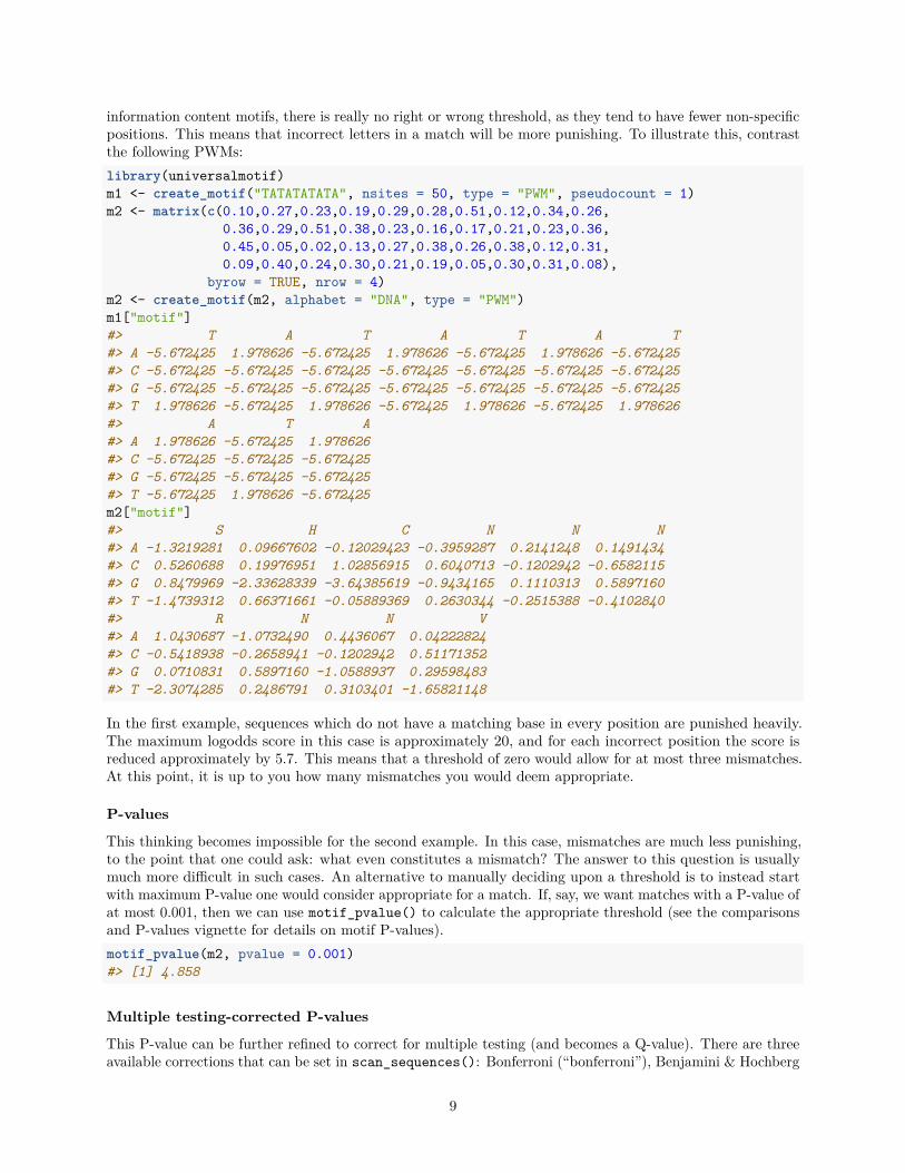
information content motifs, there is really no right or wrong threshold, as they tend to have fewer non-specificpositions. This means that incorrect letters in a match will be more punishing. To illustrate this, contrastthe following PWMs:library(universalmotif)m1 <- create_motif("TATATATATA", nsites = 50, type = "PWM", pseudocount = 1)m2 <- matrix(c(0.10,0.27,0.23,0.19,0.29,0.28,0.51,0.12,0.34,0.26,

0.36,0.29,0.51,0.38,0.23,0.16,0.17,0.21,0.23,0.36,0.45,0.05,0.02,0.13,0.27,0.38,0.26,0.38,0.12,0.31,0.09,0.40,0.24,0.30,0.21,0.19,0.05,0.30,0.31,0.08),

byrow = TRUE, nrow = 4)m2 <- create_motif(m2, alphabet = "DNA", type = "PWM")m1["motif"]#> T A T A T A T#> A -5.672425 1.978626 -5.672425 1.978626 -5.672425 1.978626 -5.672425#> C -5.672425 -5.672425 -5.672425 -5.672425 -5.672425 -5.672425 -5.672425#> G -5.672425 -5.672425 -5.672425 -5.672425 -5.672425 -5.672425 -5.672425#> T 1.978626 -5.672425 1.978626 -5.672425 1.978626 -5.672425 1.978626#> A T A#> A 1.978626 -5.672425 1.978626#> C -5.672425 -5.672425 -5.672425#> G -5.672425 -5.672425 -5.672425#> T -5.672425 1.978626 -5.672425m2["motif"]#> S H C N N N#> A -1.3219281 0.09667602 -0.12029423 -0.3959287 0.2141248 0.1491434#> C 0.5260688 0.19976951 1.02856915 0.6040713 -0.1202942 -0.6582115#> G 0.8479969 -2.33628339 -3.64385619 -0.9434165 0.1110313 0.5897160#> T -1.4739312 0.66371661 -0.05889369 0.2630344 -0.2515388 -0.4102840#> R N N V#> A 1.0430687 -1.0732490 0.4436067 0.04222824#> C -0.5418938 -0.2658941 -0.1202942 0.51171352#> G 0.0710831 0.5897160 -1.0588937 0.29598483#> T -2.3074285 0.2486791 0.3103401 -1.65821148

In the first example, sequences which do not have a matching base in every position are punished heavily.The maximum logodds score in this case is approximately 20, and for each incorrect position the score isreduced approximately by 5.7. This means that a threshold of zero would allow for at most three mismatches.At this point, it is up to you how many mismatches you would deem appropriate.

P-values

This thinking becomes impossible for the second example. In this case, mismatches are much less punishing,to the point that one could ask: what even constitutes a mismatch? The answer to this question is usuallymuch more difficult in such cases. An alternative to manually deciding upon a threshold is to instead startwith maximum P-value one would consider appropriate for a match. If, say, we want matches with a P-value ofat most 0.001, then we can use motif_pvalue() to calculate the appropriate threshold (see the comparisonsand P-values vignette for details on motif P-values).motif_pvalue(m2, pvalue = 0.001)#> [1] 4.858

Multiple testing-corrected P-values

This P-value can be further refined to correct for multiple testing (and becomes a Q-value). There are threeavailable corrections that can be set in scan_sequences(): Bonferroni (“bonferroni”), Benjamini & Hochberg

9

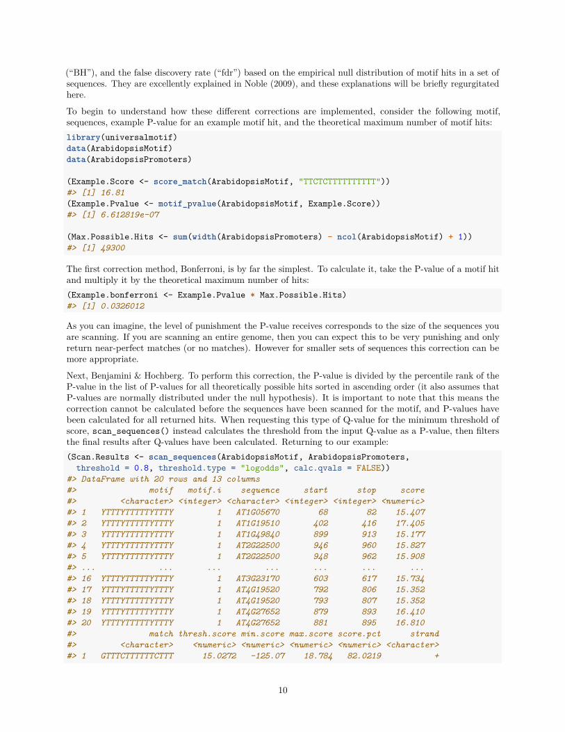
(“BH”), and the false discovery rate (“fdr”) based on the empirical null distribution of motif hits in a set ofsequences. They are excellently explained in Noble (2009), and these explanations will be briefly regurgitatedhere.

To begin to understand how these different corrections are implemented, consider the following motif,sequences, example P-value for an example motif hit, and the theoretical maximum number of motif hits:library(universalmotif)data(ArabidopsisMotif)data(ArabidopsisPromoters)

(Example.Score <- score_match(ArabidopsisMotif, "TTCTCTTTTTTTTTT"))#> [1] 16.81(Example.Pvalue <- motif_pvalue(ArabidopsisMotif, Example.Score))#> [1] 6.612819e-07

(Max.Possible.Hits <- sum(width(ArabidopsisPromoters) - ncol(ArabidopsisMotif) + 1))#> [1] 49300

The first correction method, Bonferroni, is by far the simplest. To calculate it, take the P-value of a motif hitand multiply it by the theoretical maximum number of hits:(Example.bonferroni <- Example.Pvalue * Max.Possible.Hits)#> [1] 0.0326012

As you can imagine, the level of punishment the P-value receives corresponds to the size of the sequences youare scanning. If you are scanning an entire genome, then you can expect this to be very punishing and onlyreturn near-perfect matches (or no matches). However for smaller sets of sequences this correction can bemore appropriate.

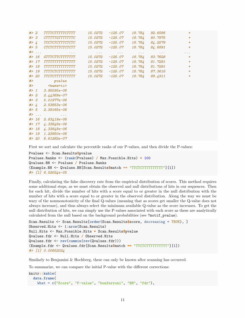
Next, Benjamini & Hochberg. To perform this correction, the P-value is divided by the percentile rank of theP-value in the list of P-values for all theoretically possible hits sorted in ascending order (it also assumes thatP-values are normally distributed under the null hypothesis). It is important to note that this means thecorrection cannot be calculated before the sequences have been scanned for the motif, and P-values havebeen calculated for all returned hits. When requesting this type of Q-value for the minimum threshold ofscore, scan_sequences() instead calculates the threshold from the input Q-value as a P-value, then filtersthe final results after Q-values have been calculated. Returning to our example:(Scan.Results <- scan_sequences(ArabidopsisMotif, ArabidopsisPromoters,

threshold = 0.8, threshold.type = "logodds", calc.qvals = FALSE))#> DataFrame with 20 rows and 13 columns#> motif motif.i sequence start stop score#> <character> <integer> <character> <integer> <integer> <numeric>#> 1 YTTTYTTTTTYTTTY 1 AT1G05670 68 82 15.407#> 2 YTTTYTTTTTYTTTY 1 AT1G19510 402 416 17.405#> 3 YTTTYTTTTTYTTTY 1 AT1G49840 899 913 15.177#> 4 YTTTYTTTTTYTTTY 1 AT2G22500 946 960 15.827#> 5 YTTTYTTTTTYTTTY 1 AT2G22500 948 962 15.908#> ... ... ... ... ... ... ...#> 16 YTTTYTTTTTYTTTY 1 AT3G23170 603 617 15.734#> 17 YTTTYTTTTTYTTTY 1 AT4G19520 792 806 15.352#> 18 YTTTYTTTTTYTTTY 1 AT4G19520 793 807 15.352#> 19 YTTTYTTTTTYTTTY 1 AT4G27652 879 893 16.410#> 20 YTTTYTTTTTYTTTY 1 AT4G27652 881 895 16.810#> match thresh.score min.score max.score score.pct strand#> <character> <numeric> <numeric> <numeric> <numeric> <character>#> 1 GTTTCTTTTTTCTTT 15.0272 -125.07 18.784 82.0219 +

10

#> 2 TTTTCTTTTTCTTTT 15.0272 -125.07 18.784 92.6586 +#> 3 CTTTTTGTTTTTTTC 15.0272 -125.07 18.784 80.7975 +#> 4 TCCTCTCTTTCTCTC 15.0272 -125.07 18.784 84.2579 +#> 5 CTCTCTTTCTCTCTT 15.0272 -125.07 18.784 84.6891 +#> ... ... ... ... ... ... ...#> 16 GTTTCTTCTTTTTTT 15.0272 -125.07 18.784 83.7628 +#> 17 TTTTTTTTTTTTTTT 15.0272 -125.07 18.784 81.7291 +#> 18 TTTTTTTTTTTTTTT 15.0272 -125.07 18.784 81.7291 +#> 19 TTTTCTCTTTTTTTT 15.0272 -125.07 18.784 87.3616 +#> 20 TTCTCTTTTTTTTTT 15.0272 -125.07 18.784 89.4911 +#> pvalue#> <numeric>#> 1 3.95595e-06#> 2 2.44369e-07#> 3 5.01977e-06#> 4 2.53853e-06#> 5 2.39165e-06#> ... ...#> 16 2.83419e-06#> 17 4.33848e-06#> 18 4.33848e-06#> 19 1.23950e-06#> 20 6.61282e-07

First we sort and calculate the percentile ranks of our P-values, and then divide the P-values:Pvalues <- Scan.Results$pvaluePvalues.Ranks <- (rank(Pvalues) / Max.Possible.Hits) * 100Qvalues.BH <- Pvalues / Pvalues.Ranks(Example.BH <- Qvalues.BH[Scan.Results$match == "TTCTCTTTTTTTTTT"][1])#> [1] 6.52024e-05

Finally, calculating the false discovery rate from the empirical distribution of scores. This method requiressome additional steps, as we must obtain the observed and null distributions of hits in our sequences. Thenfor each hit, divide the number of hits with a score equal to or greater in the null distribution with thenumber of hits with a score equal to or greater in the observed distribution. Along the way we must bewary of the nonmonotonicity of the final Q-values (meaning that as scores get smaller the Q-value does notalways increase), and thus always select the minimum available Q-value as the score increases. To get thenull distribution of hits, we can simply use the P-values associated with each score as these are analyticallycalculated from the null based on the background probabilities (see ?motif_pvalue).Scan.Results <- Scan.Results[order(Scan.Results$score, decreasing = TRUE), ]Observed.Hits <- 1:nrow(Scan.Results)Null.Hits <- Max.Possible.Hits * Scan.Results$pvalueQvalues.fdr <- Null.Hits / Observed.HitsQvalues.fdr <- rev(cummin(rev(Qvalues.fdr)))(Example.fdr <- Qvalues.fdr[Scan.Results$match == "TTCTCTTTTTTTTTT"][1])#> [1] 0.00652024

Similarly to Benjamini & Hochberg, these can only be known after scanning has occurred.

To summarize, we can compare the initial P-value with the different corrections:knitr::kable(

data.frame(What = c("Score", "P-value", "bonferroni", "BH", "fdr"),

11

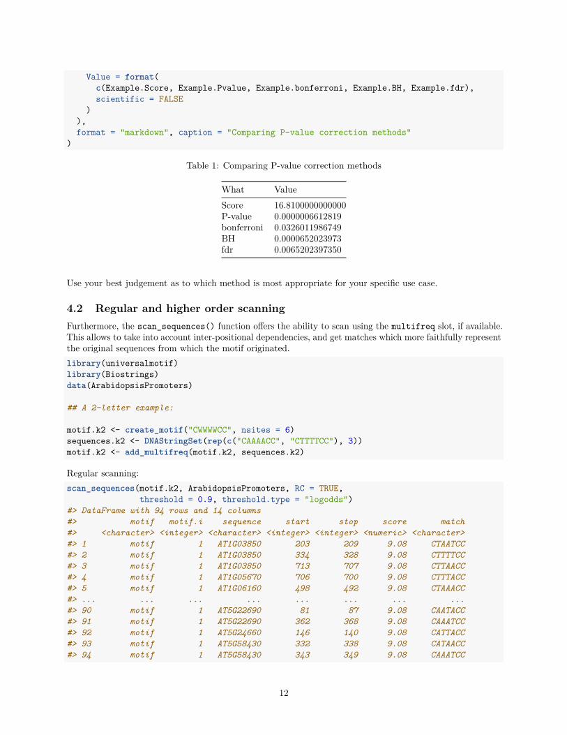
Value = format(c(Example.Score, Example.Pvalue, Example.bonferroni, Example.BH, Example.fdr),scientific = FALSE

)),format = "markdown", caption = "Comparing P-value correction methods"

)

Table 1: Comparing P-value correction methods

What ValueScore 16.8100000000000P-value 0.0000006612819bonferroni 0.0326011986749BH 0.0000652023973fdr 0.0065202397350

Use your best judgement as to which method is most appropriate for your specific use case.

4.2 Regular and higher order scanningFurthermore, the scan_sequences() function offers the ability to scan using the multifreq slot, if available.This allows to take into account inter-positional dependencies, and get matches which more faithfully representthe original sequences from which the motif originated.library(universalmotif)library(Biostrings)data(ArabidopsisPromoters)

## A 2-letter example:

motif.k2 <- create_motif("CWWWWCC", nsites = 6)sequences.k2 <- DNAStringSet(rep(c("CAAAACC", "CTTTTCC"), 3))motif.k2 <- add_multifreq(motif.k2, sequences.k2)

Regular scanning:scan_sequences(motif.k2, ArabidopsisPromoters, RC = TRUE,

threshold = 0.9, threshold.type = "logodds")#> DataFrame with 94 rows and 14 columns#> motif motif.i sequence start stop score match#> <character> <integer> <character> <integer> <integer> <numeric> <character>#> 1 motif 1 AT1G03850 203 209 9.08 CTAATCC#> 2 motif 1 AT1G03850 334 328 9.08 CTTTTCC#> 3 motif 1 AT1G03850 713 707 9.08 CTTAACC#> 4 motif 1 AT1G05670 706 700 9.08 CTTTACC#> 5 motif 1 AT1G06160 498 492 9.08 CTAAACC#> ... ... ... ... ... ... ... ...#> 90 motif 1 AT5G22690 81 87 9.08 CAATACC#> 91 motif 1 AT5G22690 362 368 9.08 CAAATCC#> 92 motif 1 AT5G24660 146 140 9.08 CATTACC#> 93 motif 1 AT5G58430 332 338 9.08 CATAACC#> 94 motif 1 AT5G58430 343 349 9.08 CAAATCC

12

#> thresh.score min.score max.score score.pct strand pvalue#> <numeric> <numeric> <numeric> <numeric> <character> <numeric>#> 1 8.172 -19.649 9.08 100 + 0.000976562#> 2 8.172 -19.649 9.08 100 - 0.000976562#> 3 8.172 -19.649 9.08 100 - 0.000976562#> 4 8.172 -19.649 9.08 100 - 0.000976562#> 5 8.172 -19.649 9.08 100 - 0.000976562#> ... ... ... ... ... ... ...#> 90 8.172 -19.649 9.08 100 + 0.000976562#> 91 8.172 -19.649 9.08 100 + 0.000976562#> 92 8.172 -19.649 9.08 100 - 0.000976562#> 93 8.172 -19.649 9.08 100 + 0.000976562#> 94 8.172 -19.649 9.08 100 + 0.000976562#> qvalue#> <numeric>#> 1 1#> 2 1#> 3 1#> 4 1#> 5 1#> ... ...#> 90 1#> 91 1#> 92 1#> 93 1#> 94 1

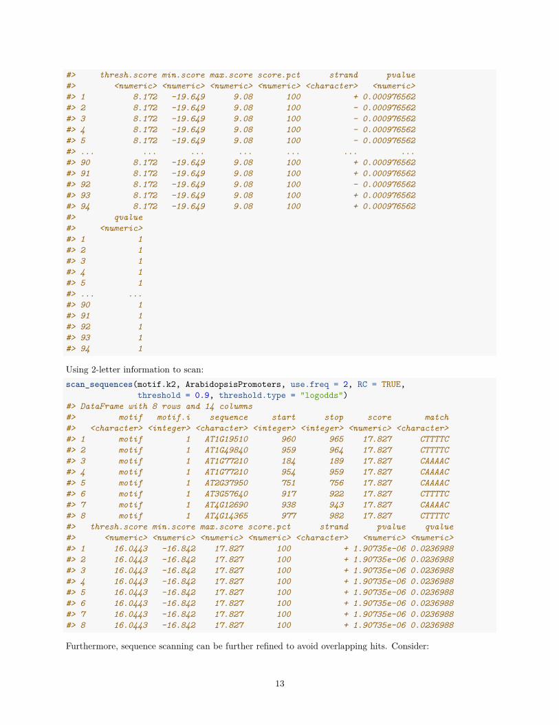
Using 2-letter information to scan:scan_sequences(motif.k2, ArabidopsisPromoters, use.freq = 2, RC = TRUE,

threshold = 0.9, threshold.type = "logodds")#> DataFrame with 8 rows and 14 columns#> motif motif.i sequence start stop score match#> <character> <integer> <character> <integer> <integer> <numeric> <character>#> 1 motif 1 AT1G19510 960 965 17.827 CTTTTC#> 2 motif 1 AT1G49840 959 964 17.827 CTTTTC#> 3 motif 1 AT1G77210 184 189 17.827 CAAAAC#> 4 motif 1 AT1G77210 954 959 17.827 CAAAAC#> 5 motif 1 AT2G37950 751 756 17.827 CAAAAC#> 6 motif 1 AT3G57640 917 922 17.827 CTTTTC#> 7 motif 1 AT4G12690 938 943 17.827 CAAAAC#> 8 motif 1 AT4G14365 977 982 17.827 CTTTTC#> thresh.score min.score max.score score.pct strand pvalue qvalue#> <numeric> <numeric> <numeric> <numeric> <character> <numeric> <numeric>#> 1 16.0443 -16.842 17.827 100 + 1.90735e-06 0.0236988#> 2 16.0443 -16.842 17.827 100 + 1.90735e-06 0.0236988#> 3 16.0443 -16.842 17.827 100 + 1.90735e-06 0.0236988#> 4 16.0443 -16.842 17.827 100 + 1.90735e-06 0.0236988#> 5 16.0443 -16.842 17.827 100 + 1.90735e-06 0.0236988#> 6 16.0443 -16.842 17.827 100 + 1.90735e-06 0.0236988#> 7 16.0443 -16.842 17.827 100 + 1.90735e-06 0.0236988#> 8 16.0443 -16.842 17.827 100 + 1.90735e-06 0.0236988

Furthermore, sequence scanning can be further refined to avoid overlapping hits. Consider:

13

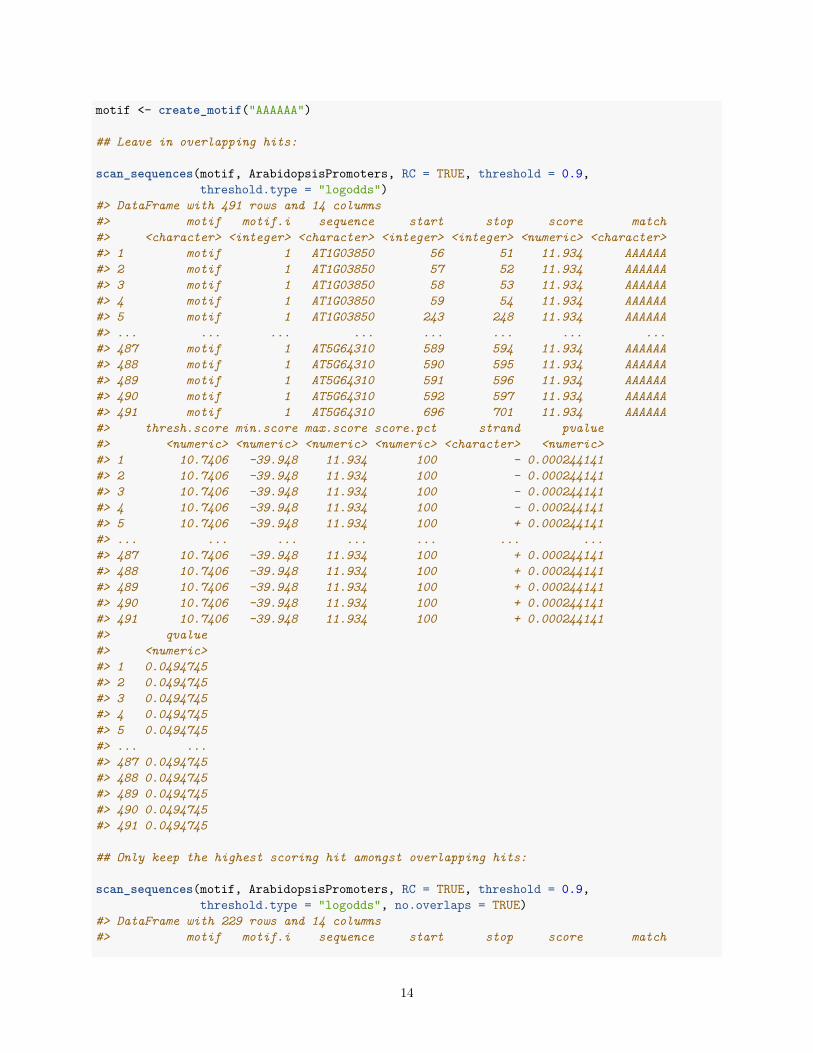
motif <- create_motif("AAAAAA")

## Leave in overlapping hits:

scan_sequences(motif, ArabidopsisPromoters, RC = TRUE, threshold = 0.9,threshold.type = "logodds")

#> DataFrame with 491 rows and 14 columns#> motif motif.i sequence start stop score match#> <character> <integer> <character> <integer> <integer> <numeric> <character>#> 1 motif 1 AT1G03850 56 51 11.934 AAAAAA#> 2 motif 1 AT1G03850 57 52 11.934 AAAAAA#> 3 motif 1 AT1G03850 58 53 11.934 AAAAAA#> 4 motif 1 AT1G03850 59 54 11.934 AAAAAA#> 5 motif 1 AT1G03850 243 248 11.934 AAAAAA#> ... ... ... ... ... ... ... ...#> 487 motif 1 AT5G64310 589 594 11.934 AAAAAA#> 488 motif 1 AT5G64310 590 595 11.934 AAAAAA#> 489 motif 1 AT5G64310 591 596 11.934 AAAAAA#> 490 motif 1 AT5G64310 592 597 11.934 AAAAAA#> 491 motif 1 AT5G64310 696 701 11.934 AAAAAA#> thresh.score min.score max.score score.pct strand pvalue#> <numeric> <numeric> <numeric> <numeric> <character> <numeric>#> 1 10.7406 -39.948 11.934 100 - 0.000244141#> 2 10.7406 -39.948 11.934 100 - 0.000244141#> 3 10.7406 -39.948 11.934 100 - 0.000244141#> 4 10.7406 -39.948 11.934 100 - 0.000244141#> 5 10.7406 -39.948 11.934 100 + 0.000244141#> ... ... ... ... ... ... ...#> 487 10.7406 -39.948 11.934 100 + 0.000244141#> 488 10.7406 -39.948 11.934 100 + 0.000244141#> 489 10.7406 -39.948 11.934 100 + 0.000244141#> 490 10.7406 -39.948 11.934 100 + 0.000244141#> 491 10.7406 -39.948 11.934 100 + 0.000244141#> qvalue#> <numeric>#> 1 0.0494745#> 2 0.0494745#> 3 0.0494745#> 4 0.0494745#> 5 0.0494745#> ... ...#> 487 0.0494745#> 488 0.0494745#> 489 0.0494745#> 490 0.0494745#> 491 0.0494745

## Only keep the highest scoring hit amongst overlapping hits:

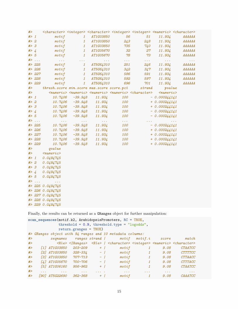
scan_sequences(motif, ArabidopsisPromoters, RC = TRUE, threshold = 0.9,threshold.type = "logodds", no.overlaps = TRUE)

#> DataFrame with 229 rows and 14 columns#> motif motif.i sequence start stop score match

14

#> <character> <integer> <character> <integer> <integer> <numeric> <character>#> 1 motif 1 AT1G03850 56 51 11.934 AAAAAA#> 2 motif 1 AT1G03850 243 248 11.934 AAAAAA#> 3 motif 1 AT1G03850 735 740 11.934 AAAAAA#> 4 motif 1 AT1G05670 32 27 11.934 AAAAAA#> 5 motif 1 AT1G05670 78 73 11.934 AAAAAA#> ... ... ... ... ... ... ... ...#> 225 motif 1 AT5G64310 251 246 11.934 AAAAAA#> 226 motif 1 AT5G64310 342 347 11.934 AAAAAA#> 227 motif 1 AT5G64310 586 591 11.934 AAAAAA#> 228 motif 1 AT5G64310 592 597 11.934 AAAAAA#> 229 motif 1 AT5G64310 696 701 11.934 AAAAAA#> thresh.score min.score max.score score.pct strand pvalue#> <numeric> <numeric> <numeric> <numeric> <character> <numeric>#> 1 10.7406 -39.948 11.934 100 - 0.000244141#> 2 10.7406 -39.948 11.934 100 + 0.000244141#> 3 10.7406 -39.948 11.934 100 + 0.000244141#> 4 10.7406 -39.948 11.934 100 - 0.000244141#> 5 10.7406 -39.948 11.934 100 - 0.000244141#> ... ... ... ... ... ... ...#> 225 10.7406 -39.948 11.934 100 - 0.000244141#> 226 10.7406 -39.948 11.934 100 + 0.000244141#> 227 10.7406 -39.948 11.934 100 + 0.000244141#> 228 10.7406 -39.948 11.934 100 + 0.000244141#> 229 10.7406 -39.948 11.934 100 + 0.000244141#> qvalue#> <numeric>#> 1 0.0494745#> 2 0.0494745#> 3 0.0494745#> 4 0.0494745#> 5 0.0494745#> ... ...#> 225 0.0494745#> 226 0.0494745#> 227 0.0494745#> 228 0.0494745#> 229 0.0494745

Finally, the results can be returned as a GRanges object for further manipulation:scan_sequences(motif.k2, ArabidopsisPromoters, RC = TRUE,

threshold = 0.9, threshold.type = "logodds",return.granges = TRUE)

#> GRanges object with 94 ranges and 10 metadata columns:#> seqnames ranges strand | motif motif.i score match#> <Rle> <IRanges> <Rle> | <character> <integer> <numeric> <character>#> [1] AT1G03850 203-209 + | motif 1 9.08 CTAATCC#> [2] AT1G03850 328-334 - | motif 1 9.08 CTTTTCC#> [3] AT1G03850 707-713 - | motif 1 9.08 CTTAACC#> [4] AT1G05670 700-706 - | motif 1 9.08 CTTTACC#> [5] AT1G06160 956-962 + | motif 1 9.08 CTAATCC#> ... ... ... ... . ... ... ... ...#> [90] AT5G22690 362-368 + | motif 1 9.08 CAAATCC

15

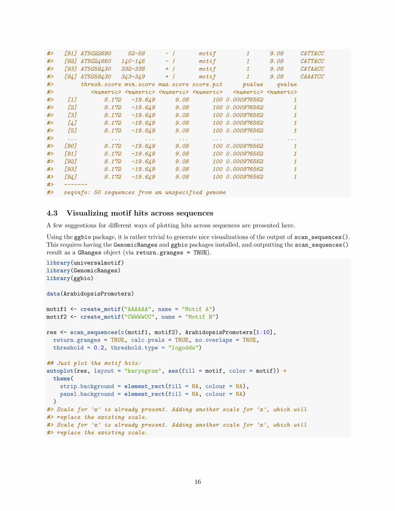
#> [91] AT5G22690 52-58 - | motif 1 9.08 CATTACC#> [92] AT5G24660 140-146 - | motif 1 9.08 CATTACC#> [93] AT5G58430 332-338 + | motif 1 9.08 CATAACC#> [94] AT5G58430 343-349 + | motif 1 9.08 CAAATCC#> thresh.score min.score max.score score.pct pvalue qvalue#> <numeric> <numeric> <numeric> <numeric> <numeric> <numeric>#> [1] 8.172 -19.649 9.08 100 0.000976562 1#> [2] 8.172 -19.649 9.08 100 0.000976562 1#> [3] 8.172 -19.649 9.08 100 0.000976562 1#> [4] 8.172 -19.649 9.08 100 0.000976562 1#> [5] 8.172 -19.649 9.08 100 0.000976562 1#> ... ... ... ... ... ... ...#> [90] 8.172 -19.649 9.08 100 0.000976562 1#> [91] 8.172 -19.649 9.08 100 0.000976562 1#> [92] 8.172 -19.649 9.08 100 0.000976562 1#> [93] 8.172 -19.649 9.08 100 0.000976562 1#> [94] 8.172 -19.649 9.08 100 0.000976562 1#> -------#> seqinfo: 50 sequences from an unspecified genome

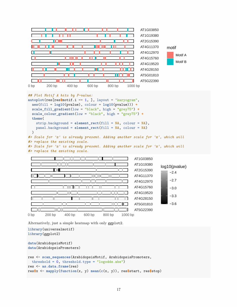
4.3 Visualizing motif hits across sequencesA few suggestions for different ways of plotting hits across sequences are presented here.

Using the ggbio package, it is rather trivial to generate nice visualizations of the output of scan_sequences().This requires having the GenomicRanges and ggbio packages installed, and outputting the scan_sequences()result as a GRanges object (via return.granges = TRUE).library(universalmotif)library(GenomicRanges)library(ggbio)

data(ArabidopsisPromoters)

motif1 <- create_motif("AAAAAA", name = "Motif A")motif2 <- create_motif("CWWWWCC", name = "Motif B")

res <- scan_sequences(c(motif1, motif2), ArabidopsisPromoters[1:10],return.granges = TRUE, calc.pvals = TRUE, no.overlaps = TRUE,threshold = 0.2, threshold.type = "logodds")

## Just plot the motif hits:autoplot(res, layout = "karyogram", aes(fill = motif, color = motif)) +

theme(strip.background = element_rect(fill = NA, colour = NA),panel.background = element_rect(fill = NA, colour = NA)

)#> Scale for 'x' is already present. Adding another scale for 'x', which will#> replace the existing scale.#> Scale for 'x' is already present. Adding another scale for 'x', which will#> replace the existing scale.

16

AT1G03850

AT1G19380

AT2G15390

AT4G11370

AT4G12970

AT4G15760

AT4G19520

AT4G28150

AT5G01810

AT5G223900 bp 200 bp 400 bp 600 bp 800 bp 1000 bp

motif

Motif A

Motif B

## Plot Motif A hits by P-value:autoplot(res[res$motif.i == 1, ], layout = "karyogram",

aes(fill = log10(pvalue), colour = log10(pvalue))) +scale_fill_gradient(low = "black", high = "grey75") +scale_colour_gradient(low = "black", high = "grey75") +theme(

strip.background = element_rect(fill = NA, colour = NA),panel.background = element_rect(fill = NA, colour = NA)

)#> Scale for 'x' is already present. Adding another scale for 'x', which will#> replace the existing scale.#> Scale for 'x' is already present. Adding another scale for 'x', which will#> replace the existing scale.

AT1G03850

AT1G19380

AT2G15390

AT4G11370

AT4G12970

AT4G15760

AT4G19520

AT4G28150

AT5G01810

AT5G223900 bp 200 bp 400 bp 600 bp 800 bp 1000 bp

−3.6

−3.3

−3.0

−2.7

−2.4

log10(pvalue)

Alternatively, just a simple heatmap with only ggplot2.library(universalmotif)library(ggplot2)

data(ArabidopsisMotif)data(ArabidopsisPromoters)

res <- scan_sequences(ArabidopsisMotif, ArabidopsisPromoters,threshold = 0, threshold.type = "logodds.abs")

res <- as.data.frame(res)res$x <- mapply(function(x, y) mean(c(x, y)), res$start, res$stop)

17

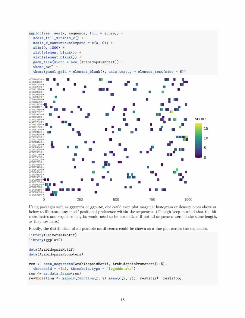
ggplot(res, aes(x, sequence, fill = score)) +scale_fill_viridis_c() +scale_x_continuous(expand = c(0, 0)) +xlim(0, 1000) +xlab(element_blank()) +ylab(element_blank()) +geom_tile(width = ncol(ArabidopsisMotif)) +theme_bw() +theme(panel.grid = element_blank(), axis.text.y = element_text(size = 6))

AT1G03850AT1G05670AT1G06160AT1G07490AT1G08090AT1G12990AT1G19380AT1G19510AT1G49120AT1G49840AT1G51700AT1G75490AT1G76590AT1G77210AT2G04025AT2G15390AT2G17450AT2G19810AT2G22500AT2G24240AT2G27690AT2G28140AT2G37950AT3G15610AT3G19200AT3G23170AT3G57640AT4G11370AT4G12690AT4G12970AT4G14365AT4G15760AT4G19520AT4G27652AT4G28150AT4G33467AT4G33970AT5G05090AT5G08790AT5G10210AT5G10695AT5G20200AT5G22390AT5G22690AT5G47230AT5G58430AT5G64310

0 250 500 750 1000

0

5

10

15

score

Using packages such as ggExtra or ggpubr, one could even plot marginal histogram or density plots above orbelow to illustrate any motif positional preference within the sequences. (Though keep in mind that the hitcoordinates and sequence lengths would need to be normalized if not all sequences were of the same length,as they are here.)

Finally, the distribution of all possible motif scores could be shown as a line plot across the sequences.library(universalmotif)library(ggplot2)

data(ArabidopsisMotif)data(ArabidopsisPromoters)

res <- scan_sequences(ArabidopsisMotif, ArabidopsisPromoters[1:5],threshold = -Inf, threshold.type = "logodds.abs")

res <- as.data.frame(res)res$position <- mapply(function(x, y) mean(c(x, y)), res$start, res$stop)

18

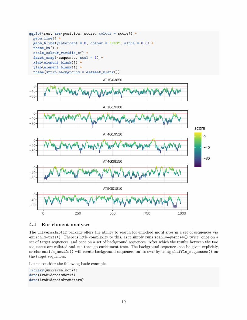
ggplot(res, aes(position, score, colour = score)) +geom_line() +geom_hline(yintercept = 0, colour = "red", alpha = 0.3) +theme_bw() +scale_colour_viridis_c() +facet_wrap(~sequence, ncol = 1) +xlab(element_blank()) +ylab(element_blank()) +theme(strip.background = element_blank())

AT5G01810

AT4G28150

AT4G19520

AT1G19380

AT1G03850

0 250 500 750 1000

−80−40

0

−80−40

0

−80−40

0

−80−40

0

−80−40

0

−80

−40

0

score

4.4 Enrichment analysesThe universalmotif package offers the ability to search for enriched motif sites in a set of sequences viaenrich_motifs(). There is little complexity to this, as it simply runs scan_sequences() twice: once on aset of target sequences, and once on a set of background sequences. After which the results between the twosequences are collated and run through enrichment tests. The background sequences can be given explicitly,or else enrich_motifs() will create background sequences on its own by using shuffle_sequences() onthe target sequences.

Let us consider the following basic example:library(universalmotif)data(ArabidopsisMotif)data(ArabidopsisPromoters)

19

enrich_motifs(ArabidopsisMotif, ArabidopsisPromoters, shuffle.k = 3,threshold = 0.001, RC = TRUE)

#> DataFrame with 1 row and 11 columns#> motif motif.i target.hits target.seq.hits target.seq.count#> <character> <integer> <integer> <integer> <integer>#> 1 YTTTYTTTTTYTTTY 1 683 50 50#> bkg.hits bkg.seq.hits bkg.seq.count Pval Qval Eval#> <integer> <integer> <integer> <numeric> <numeric> <numeric>#> 1 307 48 50 5.45519e-34 5.45519e-34 1.09104e-33

Here we can see that the motif is significantly enriched in the target sequences. The Pval was calculated bycalling stats::fisher.test().

One final point: always keep in mind the threshold parameter, as this will ultimately decide the number ofhits found. (A bad threshold can lead to a false negative.)

4.5 Fixed and variable-length gapped motifsuniversalmotif class motifs can be gapped, which can be used by scan_sequences() and enrich_motifs().Note that gapped motif support is currently limited to these two functions. All other functions will ignorethe gap information, and even discard them in functions such as merge_motifs().

First, obtain the component motifs:library(universalmotif)data(ArabidopsisPromoters)

m1 <- create_motif("TTTATAT", name = "PartA")m2 <- create_motif("GGTTCGA", name = "PartB")

Then, combine them and add the desired gap. In this case, a gap will be added between the two motifs whichcan range in size from 4-6 bases.m <- cbind(m1, m2)m <- add_gap(m, gaploc = ncol(m1), mingap = 4, maxgap = 6)m#>#> Motif name: PartA/PartB#> Alphabet: DNA#> Type: PCM#> Strands: +-#> Total IC: 28#> Pseudocount: 0#> Consensus: TTTATAT..GGTTCGA#> Gap locations: 7-8#> Gap sizes: 4-6#>#> T T T A T A T G G T T C G A#> A 0 0 0 1 0 1 0 .. 0 0 0 0 0 0 1#> C 0 0 0 0 0 0 0 .. 0 0 0 0 1 0 0#> G 0 0 0 0 0 0 0 .. 1 1 0 0 0 1 0#> T 1 1 1 0 1 0 1 .. 0 0 1 1 0 0 0

Now, it can be used directly in scan_sequences() or enrich_motifs():scan_sequences(m, ArabidopsisPromoters, threshold = 0.4, threshold.type = "logodds")#> DataFrame with 75 rows and 14 columns

20

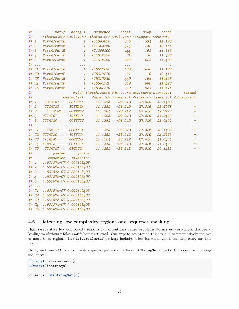
#> motif motif.i sequence start stop score#> <character> <integer> <character> <integer> <integer> <numeric>#> 1 PartA/PartB 1 AT1G03850 376 394 11.178#> 2 PartA/PartB 1 AT1G03850 414 432 12.168#> 3 PartA/PartB 1 AT1G06160 144 161 11.918#> 4 PartA/PartB 1 AT1G12990 71 90 11.428#> 5 PartA/PartB 1 AT1G19380 226 245 11.428#> ... ... ... ... ... ... ...#> 71 PartA/PartB 1 AT5G22690 638 656 11.178#> 72 PartA/PartB 1 AT5G47230 91 110 12.418#> 73 PartA/PartB 1 AT5G47230 449 468 11.428#> 74 PartA/PartB 1 AT5G64310 869 888 11.428#> 75 PartA/PartB 1 AT5G64310 909 927 11.178#> match thresh.score min.score max.score score.pct strand#> <character> <numeric> <numeric> <numeric> <numeric> <character>#> 1 TATATGT.....GGTGCAA 11.1384 -93.212 27.846 40.1422 +#> 2 TTGATAT.....TGTTAGA 11.1384 -93.212 27.846 43.6975 +#> 3 TTTATGT....GGTTTGT 11.1384 -93.212 27.846 42.7997 +#> 4 GTTATGT......TGTTAGA 11.1384 -93.212 27.846 41.0400 +#> 5 TTTACAG......CGTTCGT 11.1384 -93.212 27.846 41.0400 +#> ... ... ... ... ... ... ...#> 71 TTCATTT.....GGCTTGA 11.1384 -93.212 27.846 40.1422 +#> 72 TTTATAC......TGTTCCA 11.1384 -93.212 27.846 44.5953 +#> 73 TATATGT......GGGTCAA 11.1384 -93.212 27.846 41.0400 +#> 74 ATAATAT......CGTTAGA 11.1384 -93.212 27.846 41.0400 +#> 75 TTCATAT.....GTCACGA 11.1384 -93.212 27.846 40.1422 +#> pvalue qvalue#> <numeric> <numeric>#> 1 1.60187e-07 0.000105403#> 2 1.60187e-07 0.000105403#> 3 1.60187e-07 0.000105403#> 4 1.60187e-07 0.000105403#> 5 1.60187e-07 0.000105403#> ... ... ...#> 71 1.60187e-07 0.000105403#> 72 1.60187e-07 0.000105403#> 73 1.60187e-07 0.000105403#> 74 1.60187e-07 0.000105403#> 75 1.60187e-07 0.000105403

4.6 Detecting low complexity regions and sequence maskingHighly-repetitive low complexity regions can oftentimes cause problems during de novo motif discovery,leading to obviously false motifs being returned. One way to get around this issue is to preemptively removeor mask these regions. The universalmotif package includes a few functions which can help carry out thistask.

Using mask_seqs(), one can mask a specific pattern of letters in XStringSet objects. Consider the followingsequences:library(universalmotif)library(Biostrings)

Ex.seq <- DNAStringSet(c(

21

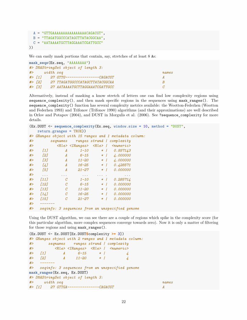
A = "GTTGAAAAAAAAAAAAAAAACAGACGT",B = "TTAGATGGCCCATAGCTTATACGGCAA",C = "AATAAAATGCTTAGGAAATCGATTGCC"

))

We can easily mask portions that contain, say, stretches of at least 8 As:mask_seqs(Ex.seq, "AAAAAAAA")#> DNAStringSet object of length 3:#> width seq names#> [1] 27 GTTG----------------CAGACGT A#> [2] 27 TTAGATGGCCCATAGCTTATACGGCAA B#> [3] 27 AATAAAATGCTTAGGAAATCGATTGCC C

Alternatively, instead of masking a know stretch of letters one can find low complexity regions usingsequence_complexity(), and then mask specific regions in the sequences using mask_ranges(). Thesequence_complexity() function has several complexity metrics available: the Wootton-Federhen (Woottonand Federhen 1993) and Trifonov (Trifonov 1990) algorithms (and their approximations) are well describedin Orlov and Potapov (2004), and DUST in Morgulis et al. (2006). See ?sequence_complexity for moredetails.(Ex.DUST <- sequence_complexity(Ex.seq, window.size = 10, method = "DUST",

return.granges = TRUE))#> GRanges object with 15 ranges and 1 metadata column:#> seqnames ranges strand | complexity#> <Rle> <IRanges> <Rle> | <numeric>#> [1] A 1-10 * | 0.857143#> [2] A 6-15 * | 4.000000#> [3] A 11-20 * | 4.000000#> [4] A 16-25 * | 0.428571#> [5] A 21-27 * | 0.000000#> ... ... ... ... . ...#> [11] C 1-10 * | 0.285714#> [12] C 6-15 * | 0.000000#> [13] C 11-20 * | 0.000000#> [14] C 16-25 * | 0.000000#> [15] C 21-27 * | 0.000000#> -------#> seqinfo: 3 sequences from an unspecified genome

Using the DUST algorithm, we can see there are a couple of regions which spike in the complexity score (forthis particular algorithm, more complex sequences converge towards zero). Now it is only a matter of filteringfor those regions and using mask_ranges().(Ex.DUST <- Ex.DUST[Ex.DUST$complexity >= 3])#> GRanges object with 2 ranges and 1 metadata column:#> seqnames ranges strand | complexity#> <Rle> <IRanges> <Rle> | <numeric>#> [1] A 6-15 * | 4#> [2] A 11-20 * | 4#> -------#> seqinfo: 3 sequences from an unspecified genomemask_ranges(Ex.seq, Ex.DUST)#> DNAStringSet object of length 3:#> width seq names#> [1] 27 GTTGA---------------CAGACGT A

22

#> [2] 27 TTAGATGGCCCATAGCTTATACGGCAA B#> [3] 27 AATAAAATGCTTAGGAAATCGATTGCC C

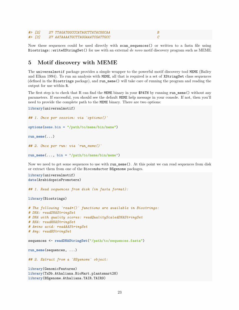
Now these sequences could be used directly with scan_sequences() or written to a fasta file usingBiostrings::writeXStringSet() for use with an external de novo motif discovery program such as MEME.

5 Motif discovery with MEMEThe universalmotif package provides a simple wrapper to the powerful motif discovery tool MEME (Baileyand Elkan 1994). To run an analysis with MEME, all that is required is a set of XStringSet class sequences(defined in the Biostrings package), and run_meme() will take care of running the program and reading theoutput for use within R.

The first step is to check that R can find the MEME binary in your $PATH by running run_meme() without anyparameters. If successful, you should see the default MEME help message in your console. If not, then you’llneed to provide the complete path to the MEME binary. There are two options:library(universalmotif)

## 1. Once per session: via `options()`

options(meme.bin = "/path/to/meme/bin/meme")

run_meme(...)

## 2. Once per run: via `run_meme()`

run_meme(..., bin = "/path/to/meme/bin/meme")

Now we need to get some sequences to use with run_meme(). At this point we can read sequences from diskor extract them from one of the Bioconductor BSgenome packages.library(universalmotif)data(ArabidopsisPromoters)

## 1. Read sequences from disk (in fasta format):

library(Biostrings)

# The following `read*()` functions are available in Biostrings:# DNA: readDNAStringSet# DNA with quality scores: readQualityScaledDNAStringSet# RNA: readRNAStringSet# Amino acid: readAAStringSet# Any: readBStringSet

sequences <- readDNAStringSet("/path/to/sequences.fasta")

run_meme(sequences, ...)

## 2. Extract from a `BSgenome` object:

library(GenomicFeatures)library(TxDb.Athaliana.BioMart.plantsmart28)library(BSgenome.Athaliana.TAIR.TAIR9)

23

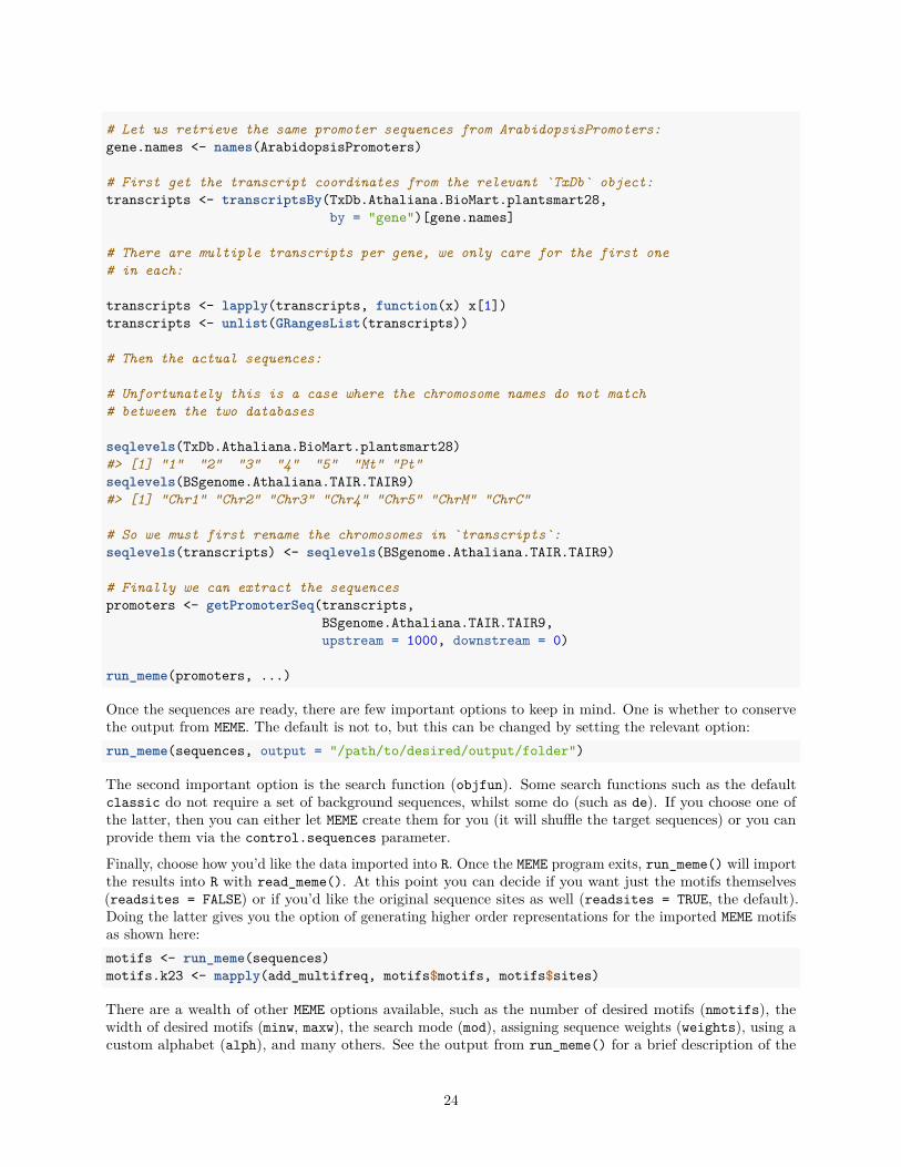
# Let us retrieve the same promoter sequences from ArabidopsisPromoters:gene.names <- names(ArabidopsisPromoters)

# First get the transcript coordinates from the relevant `TxDb` object:transcripts <- transcriptsBy(TxDb.Athaliana.BioMart.plantsmart28,

by = "gene")[gene.names]

# There are multiple transcripts per gene, we only care for the first one# in each:

transcripts <- lapply(transcripts, function(x) x[1])transcripts <- unlist(GRangesList(transcripts))

# Then the actual sequences:

# Unfortunately this is a case where the chromosome names do not match# between the two databases

seqlevels(TxDb.Athaliana.BioMart.plantsmart28)#> [1] "1" "2" "3" "4" "5" "Mt" "Pt"seqlevels(BSgenome.Athaliana.TAIR.TAIR9)#> [1] "Chr1" "Chr2" "Chr3" "Chr4" "Chr5" "ChrM" "ChrC"

# So we must first rename the chromosomes in `transcripts`:seqlevels(transcripts) <- seqlevels(BSgenome.Athaliana.TAIR.TAIR9)

# Finally we can extract the sequencespromoters <- getPromoterSeq(transcripts,

BSgenome.Athaliana.TAIR.TAIR9,upstream = 1000, downstream = 0)

run_meme(promoters, ...)

Once the sequences are ready, there are few important options to keep in mind. One is whether to conservethe output from MEME. The default is not to, but this can be changed by setting the relevant option:run_meme(sequences, output = "/path/to/desired/output/folder")

The second important option is the search function (objfun). Some search functions such as the defaultclassic do not require a set of background sequences, whilst some do (such as de). If you choose one ofthe latter, then you can either let MEME create them for you (it will shuffle the target sequences) or you canprovide them via the control.sequences parameter.

Finally, choose how you’d like the data imported into R. Once the MEME program exits, run_meme() will importthe results into R with read_meme(). At this point you can decide if you want just the motifs themselves(readsites = FALSE) or if you’d like the original sequence sites as well (readsites = TRUE, the default).Doing the latter gives you the option of generating higher order representations for the imported MEME motifsas shown here:motifs <- run_meme(sequences)motifs.k23 <- mapply(add_multifreq, motifs$motifs, motifs$sites)

There are a wealth of other MEME options available, such as the number of desired motifs (nmotifs), thewidth of desired motifs (minw, maxw), the search mode (mod), assigning sequence weights (weights), using acustom alphabet (alph), and many others. See the output from run_meme() for a brief description of the

24

options, or visit the online manual for more details.

6 Miscellaneous string utilitiesSince biological sequences are usually contained in XStringSet class objects, sequence_complexity(),get_bkg() and shuffle_sequences() are designed to work with such objects. For cases when strings arenot XStringSet objects, the following functions are available:

• calc_complexity(): alternative to sequence_complexity()• count_klets(): alternative to get_bkg()• shuffle_string(): alternative to shuffle_sequences()

library(universalmotif)

string <- "DASDSDDSASDSSA"

calc_complexity(string)#> [1] 0.7823323

count_klets(string, 2)#> klets counts#> 1 AA 0#> 2 AD 0#> 3 AS 2#> 4 DA 1#> 5 DD 1#> 6 DS 3#> 7 SA 2#> 8 SD 3#> 9 SS 1

shuffle_string(string, 2)#> [1] "DSDSDSSDDASASA"

A few other utilities have also been made available (based on the internal code of other universalmotiffunctions) that work on simple character vectors:

• calc_windows(): calculate the coordinates for sliding windows from 1 to any number n• get_klets(): get a list of all possible k-lets for any sequence alphabet• slide_fun(): apply a function over sliding windows across a single string• window_string(): retrieve characters from sliding windows of a single string

library(universalmotif)

calc_windows(n = 12, window = 4, overlap = 2)#> start stop#> 1 1 4#> 2 3 6#> 3 5 8#> 4 7 10#> 5 9 12

get_klets(c("A", "S", "D"), 2)#> [1] "AA" "AS" "AD" "SA" "SS" "SD" "DA" "DS" "DD"

slide_fun("ABCDEFGH", charToRaw, raw(2), window = 2, overlap = 1)

25

#> [,1] [,2] [,3] [,4] [,5] [,6] [,7]#> [1,] 41 42 43 44 45 46 47#> [2,] 42 43 44 45 46 47 48

window_string("ABCDEFGH", window = 2, overlap = 1)#> [1] "AB" "BC" "CD" "DE" "EF" "FG" "GH"

Session info#> R version 4.1.2 (2021-11-01)#> Platform: x86_64-pc-linux-gnu (64-bit)#> Running under: Ubuntu 20.04.3 LTS#>#> Matrix products: default#> BLAS: /home/biocbuild/bbs-3.14-bioc/R/lib/libRblas.so#> LAPACK: /home/biocbuild/bbs-3.14-bioc/R/lib/libRlapack.so#>#> locale:#> [1] LC_CTYPE=en_US.UTF-8 LC_NUMERIC=C#> [3] LC_TIME=en_GB LC_COLLATE=C#> [5] LC_MONETARY=en_US.UTF-8 LC_MESSAGES=en_US.UTF-8#> [7] LC_PAPER=en_US.UTF-8 LC_NAME=C#> [9] LC_ADDRESS=C LC_TELEPHONE=C#> [11] LC_MEASUREMENT=en_US.UTF-8 LC_IDENTIFICATION=C#>#> attached base packages:#> [1] stats4 stats graphics grDevices utils datasets methods#> [8] base#>#> other attached packages:#> [1] ggbio_1.42.0 TFBSTools_1.32.0 cowplot_1.1.1#> [4] dplyr_1.0.7 ggtree_3.2.1 ggplot2_3.3.5#> [7] MotifDb_1.36.0 GenomicRanges_1.46.1 Biostrings_2.62.0#> [10] GenomeInfoDb_1.30.0 XVector_0.34.0 IRanges_2.28.0#> [13] S4Vectors_0.32.3 BiocGenerics_0.40.0 universalmotif_1.12.2#>#> loaded via a namespace (and not attached):#> [1] backports_1.4.1 Hmisc_4.6-0#> [3] BiocFileCache_2.2.0 plyr_1.8.6#> [5] lazyeval_0.2.2 splines_4.1.2#> [7] BiocParallel_1.28.3 digest_0.6.29#> [9] ensembldb_2.18.2 yulab.utils_0.0.4#> [11] htmltools_0.5.2 GO.db_3.14.0#> [13] fansi_0.5.0 magrittr_2.0.1#> [15] checkmate_2.0.0 memoise_2.0.1#> [17] BSgenome_1.62.0 grImport2_0.2-0#> [19] cluster_2.1.2 tzdb_0.2.0#> [21] readr_2.1.1 annotate_1.72.0#> [23] matrixStats_0.61.0 R.utils_2.11.0#> [25] prettyunits_1.1.1 jpeg_0.1-9#> [27] colorspace_2.0-2 rappdirs_0.3.3#> [29] blob_1.2.2 xfun_0.29#> [31] crayon_1.4.2 RCurl_1.98-1.5

26

#> [33] jsonlite_1.7.2 graph_1.72.0#> [35] TFMPvalue_0.0.8 VariantAnnotation_1.40.0#> [37] survival_3.2-13 ape_5.6#> [39] glue_1.6.0 gtable_0.3.0#> [41] zlibbioc_1.40.0 DelayedArray_0.20.0#> [43] scales_1.1.1 DBI_1.1.2#> [45] GGally_2.1.2 Rcpp_1.0.7#> [47] viridisLite_0.4.0 progress_1.2.2#> [49] xtable_1.8-4 htmlTable_2.3.0#> [51] gridGraphics_0.5-1 tidytree_0.3.6#> [53] foreign_0.8-81 bit_4.0.4#> [55] OrganismDbi_1.36.0 Formula_1.2-4#> [57] htmlwidgets_1.5.4 httr_1.4.2#> [59] RColorBrewer_1.1-2 ellipsis_0.3.2#> [61] pkgconfig_2.0.3 reshape_0.8.8#> [63] XML_3.99-0.8 R.methodsS3_1.8.1#> [65] farver_2.1.0 dbplyr_2.1.1#> [67] nnet_7.3-16 ggseqlogo_0.1#> [69] utf8_1.2.2 ggplotify_0.1.0#> [71] tidyselect_1.1.1 labeling_0.4.2#> [73] rlang_0.4.12 reshape2_1.4.4#> [75] AnnotationDbi_1.56.2 munsell_0.5.0#> [77] tools_4.1.2 cachem_1.0.6#> [79] DirichletMultinomial_1.36.0 generics_0.1.1#> [81] RSQLite_2.2.9 ade4_1.7-18#> [83] evaluate_0.14 stringr_1.4.0#> [85] fastmap_1.1.0 yaml_2.2.1#> [87] knitr_1.37 bit64_4.0.5#> [89] caTools_1.18.2 purrr_0.3.4#> [91] AnnotationFilter_1.18.0 KEGGREST_1.34.0#> [93] splitstackshape_1.4.8 RBGL_1.70.0#> [95] nlme_3.1-153 R.oo_1.24.0#> [97] poweRlaw_0.70.6 aplot_0.1.1#> [99] xml2_1.3.3 pracma_2.3.6#> [101] biomaRt_2.50.1 rstudioapi_0.13#> [103] compiler_4.1.2 filelock_1.0.2#> [105] curl_4.3.2 png_0.1-7#> [107] treeio_1.18.1 tibble_3.1.6#> [109] stringi_1.7.6 highr_0.9#> [111] GenomicFeatures_1.46.3 lattice_0.20-45#> [113] ProtGenerics_1.26.0 CNEr_1.30.0#> [115] Matrix_1.4-0 vctrs_0.3.8#> [117] pillar_1.6.4 lifecycle_1.0.1#> [119] BiocManager_1.30.16 data.table_1.14.2#> [121] bitops_1.0-7 patchwork_1.1.1#> [123] rtracklayer_1.54.0 R6_2.5.1#> [125] BiocIO_1.4.0 latticeExtra_0.6-29#> [127] bookdown_0.24 gridExtra_2.3#> [129] motifStack_1.38.0 dichromat_2.0-0#> [131] MASS_7.3-54 gtools_3.9.2#> [133] assertthat_0.2.1 seqLogo_1.60.0#> [135] SummarizedExperiment_1.24.0 rjson_0.2.20#> [137] withr_2.4.3 GenomicAlignments_1.30.0#> [139] Rsamtools_2.10.0 GenomeInfoDbData_1.2.7

27

#> [141] parallel_4.1.2 hms_1.1.1#> [143] grid_4.1.2 rpart_4.1-15#> [145] ggfun_0.0.4 tidyr_1.1.4#> [147] rmarkdown_2.11 MatrixGenerics_1.6.0#> [149] biovizBase_1.42.0 Biobase_2.54.0#> [151] base64enc_0.1-3 tinytex_0.36#> [153] restfulr_0.0.13

ReferencesAltschul, Stephen F., and Bruce W. Erickson. 1985. “Significance of Nucleotide Sequence Alignments: AMethod for Random Sequence Permutation That Preserves Dinucleotide and Codon Usage.” MolecularBiology and Evolution 2 (6): 526–38.

Bailey, T.L., and C. Elkan. 1994. “Fitting a Mixture Model by Expectation Maximization to Discover Motifsin Biopolymers.” Proceedings of the Second International Conference on Intelligent Systems for MolecularBiology 2: 28–36.

Fitch, Walter M. 1983. “Random Sequences.” Journal of Molecular Biology 163 (2): 171–76.

Jiang, M., J. Anderson, J. Gillespie, and M. Mayne. 2008. “uShuffle: A Useful Tool for Shuffling BiologicalSequences While Preserving K-Let Counts.” BMC Bioinformatics 9 (192).

Morgulis, A., E.M. Gertz, A.A. Schaffer, and R. Agarwala. 2006. “A Fast and Symmetric DUST Implemen-tation to Mask Low-Complexity Dna Sequences.” Journal of Computational Biology 13: 1028–40.

Noble, William S. 2009. “How Does Multiple Testing Correction Work?” Nature Biotechnology 27 (12):1135–7.

Orlov, Y.L., and V.N. Potapov. 2004. “Complexity: An Internet Resource for Analysis of DNA SequenceComplexity.” Nucleic Acids Research 32: W628–W633.

Propp, J.G., and D.W. Wilson. 1998. “How to Get a Perfectly Random Sample from a Generic MarkovChain and Generate a Random Spanning Tree of a Directed Graph.” Journal of Algorithms 27: 170–217.

Trifonov, E.N. 1990. “Making Sense of the Human Genome.” In Structure & Methods, edited by R.H. Sarma,69–77. Albany: Adenine Press.

Wootton, J.C., and S. Federhen. 1993. “Statistics of Local Complexity in Amino Acid Sequences and SequenceDatabases.” Computers & Chemistry 17: 149–63.

28