Bioconductor TutorialPart I

www.bioconductor.org

Sandrine DudoitRobert Gentleman

MGED6September 3-5, 2003

Aix-en-Provence, France

Core Development TeamDouglas Bates, University of Wisconsin, Madison,USA. Benjamin Bolstad, Division of Biostatistics, UC Berkeley, USA.Vincent Carey, Harvard Medical School, USA. Marcel Dettling, Federal Inst. Technology, Switzerland. Sandrine Dudoit, Division of Biostatistics, UC Berkeley, USA. Byron Ellis, Department of Statistics, Harvard University, USA. Laurent Gautier, Technical University of Denmark, Denmark.Robert Gentleman, Harvard Medical School, USA. Jeff Gentry, Dana-Farber Cancer Institute, USA. Kurt Hornik, Technische Universitat Wien, Austria. Torsten Hothorn, Institut fuer Medizininformatik, Biometrie und Epidemiologie, Germany. Wolfgang Huber, DKFZ Heidelberg, Germany. Stefano Iacus, University of Milan, Italy Rafael Irizarry, Department of Biostatistics, Johns Hopkins University, USA. Friedrich Leisch, Technische Universitat Wien, Austria. Martin Maechler, Federal Inst. Technology, Switzerland. Colin Smith, NASA Center for Astrobioinformatics, USA. Gordon Smyth, Walter and Eliza Hall Institute, Australia. Anthony Rossini, University of Washington, Fred Hutchinson Cancer Research Center, USA.Gunther Sawitzki, Institute fur Angewandte Mathematik, Germany. Luke Tierney, University of Iowa, USA.Yee Hwa (Jean) Yang, Department of Biostatistics, UC San Francisco, USA. Jianhua (John) Zhang, Dana-Farber Cancer Institute, USA.

References• Bioconductor www.bioconductor.org

– software, data, and documentation (vignettes); – training materials from short courses; – mailing list.

• R www.r-project.org, cran.r-project.org– software (CRAN); – documentation; – newsletter: R News;– mailing list.

• Personal– www.stat.berkeley.edu/~sandrine– www.hsph.harvard.edu/facres/gent.html

OutlinePart I• Overview of the Bioconductor Project.• Getting started.• Pre-processing microarray data: Affymetrix and

spotted arrays.• Differential gene expression.• Distances, prediction, and cluster analysis.Part II• Reproducible research.• Annotation and metadata.• Visualization.• GO: more advanced usage.

Overview of the Bioconductor Project

Bioconductor• Bioconductor is an open source and open

development software project for the analysis of biomedical and genomic data.

• The project was started in the Fall of 2001 and includes 23 core developers in the US, Europe, and Australia.

• R and the R package system are used to design and distribute software.

• Releases– v 1.0: May 2nd, 2002, 15 packages.– v 1.1: November 18th, 2002, 20 packages.– v 1.2: May 28th, 2003, 30 packages.

• ArrayAnalyzer: Commercial port of Bioconductorpackages in S-Plus.

Goals• Provide access to powerful statistical and

graphical methods for the analysis of genomic data.

• Facilitate the integration of biological metadata(GenBank, GO, LocusLink, PubMed) in the analysis of experimental data.

• Allow the rapid development of extensible, interoperable, and scalable software.

• Promote high-quality documentation and reproducible research.

• Provide training in computational and statistical methods.

Bioconductor packages• Bioconductor software consists of R add-on

packages. • An R package is a structured collection of code

(R, C, or other), documentation, and/or data for performing specific types of analyses.

• E.g. affy, cluster, graph, hexbin packages provide implementations of specialized statistical and graphical methods.

Bioconductor packagesBioconductor provides two main classes of software packages.

• End-user packages: – aimed at users unfamiliar with R or computer

programming; – polished and easy-to-use interfaces to a wide variety

of computational and statistical methods for the analysis of genomic data.

• Developer packages: aimed at software developers, in the sense that they provide software to write software.

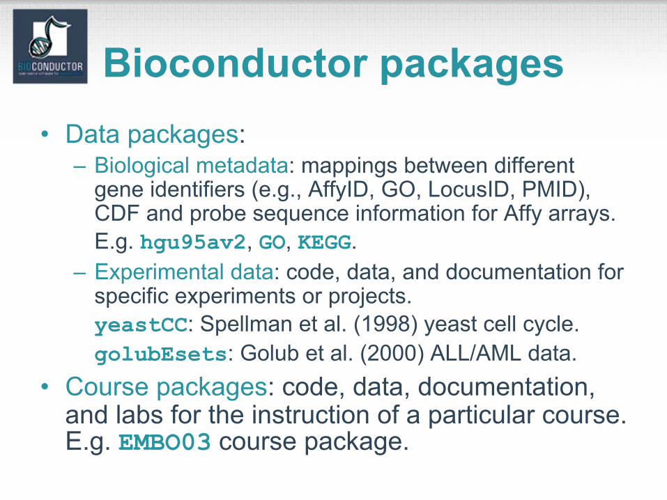
Bioconductor packages• Data packages:

– Biological metadata: mappings between different gene identifiers (e.g., AffyID, GO, LocusID, PMID), CDF and probe sequence information for Affy arrays.E.g. hgu95av2, GO, KEGG.

– Experimental data: code, data, and documentation for specific experiments or projects.yeastCC: Spellman et al. (1998) yeast cell cycle. golubEsets: Golub et al. (2000) ALL/AML data.

• Course packages: code, data, documentation, and labs for the instruction of a particular course. E.g. EMBO03 course package.

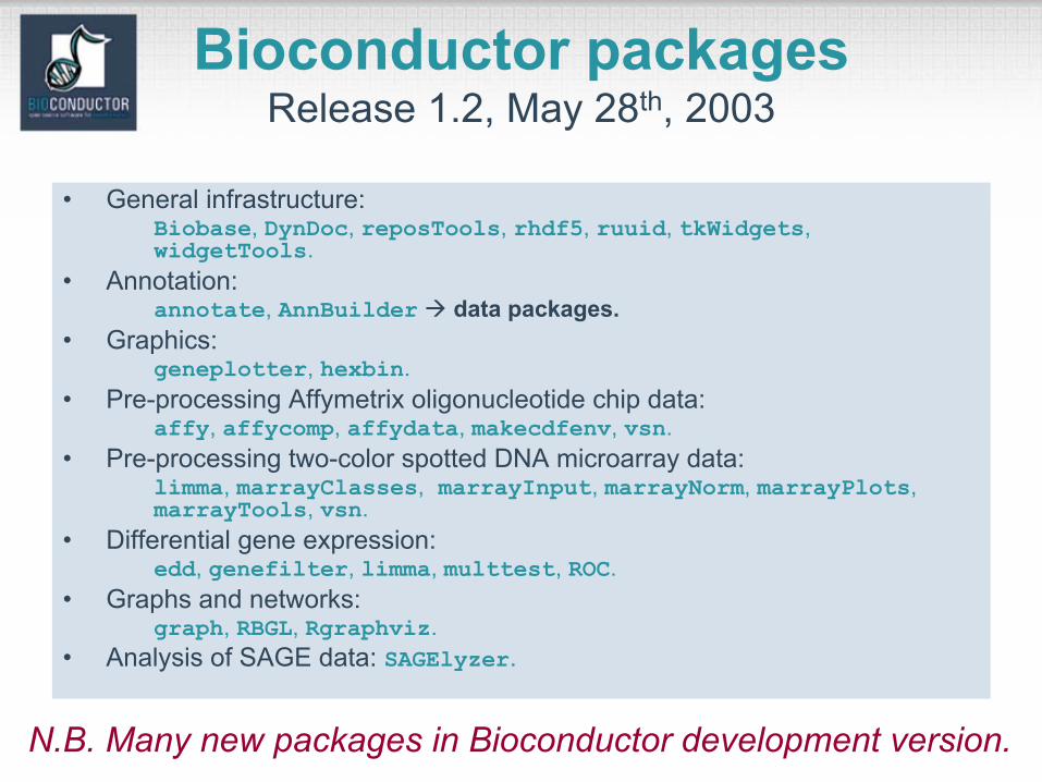
Bioconductor packagesRelease 1.2, May 28th, 2003

• General infrastructure:Biobase, DynDoc, reposTools, rhdf5, ruuid, tkWidgets,widgetTools.

• Annotation:annotate, AnnBuilder data packages.

• Graphics: geneplotter, hexbin.

• Pre-processing Affymetrix oligonucleotide chip data: affy, affycomp, affydata, makecdfenv, vsn.

• Pre-processing two-color spotted DNA microarray data: limma, marrayClasses, marrayInput, marrayNorm, marrayPlots,marrayTools, vsn.

• Differential gene expression: edd, genefilter, limma, multtest, ROC.

• Graphs and networks:graph, RBGL, Rgraphviz.

• Analysis of SAGE data: SAGElyzer.

N.B. Many new packages in Bioconductor development version.

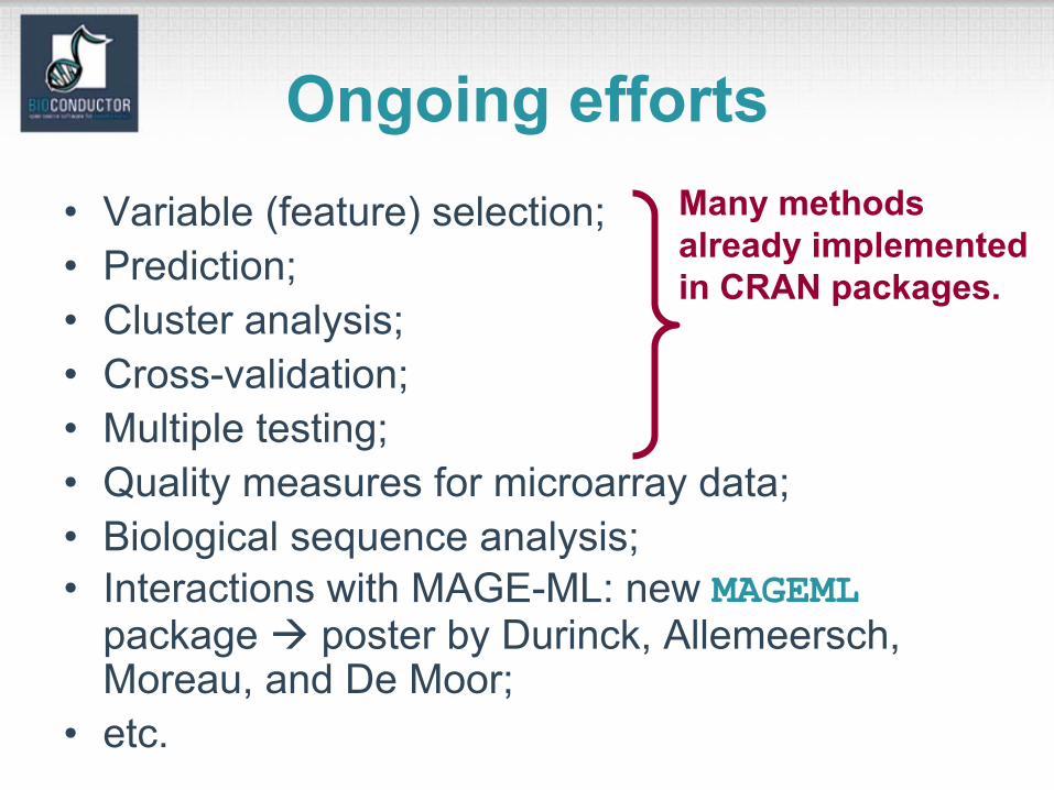
Ongoing efforts• Variable (feature) selection;• Prediction;• Cluster analysis;• Cross-validation;• Multiple testing;• Quality measures for microarray data;• Biological sequence analysis;• Interactions with MAGE-ML: new MAGEML

package poster by Durinck, Allemeersch, Moreau, and De Moor;

• etc.

Many methodsalready implementedin CRAN packages.

Microarray data analysisCEL, CDF

affyvsn

.gpr, .Spot

Pre-processing

exprSet

graphRBGL

Rgraphviz

eddgenefilter

limmamulttest

ROC+ CRAN

annotateannaffy

+ metadata packagesCRAN

classclusterMASSmva

geneplotterhexbin

+ CRAN

marraylimma

vsn

Differential expression

Graphs &networks

Clusteranalysis

Annotation

CRANclasse1071ipred

LogitBoostMASSnnet

randomForestrpart

Prediction

Graphics

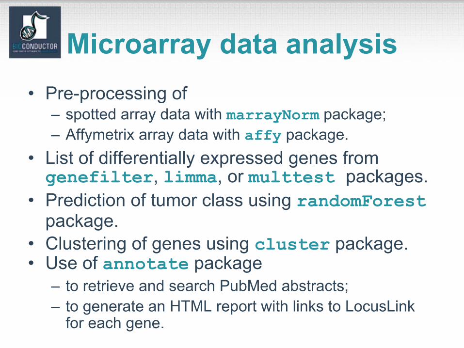
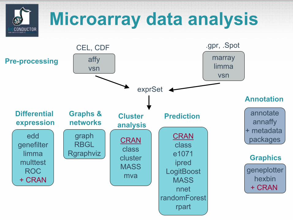
Microarray data analysis• Pre-processing of

– spotted array data with marrayNorm package;– Affymetrix array data with affy package.

• List of differentially expressed genes from genefilter, limma, or multtest packages.

• Prediction of tumor class using randomForestpackage.

• Clustering of genes using cluster package.• Use of annotate package

– to retrieve and search PubMed abstracts;– to generate an HTML report with links to LocusLink

for each gene.

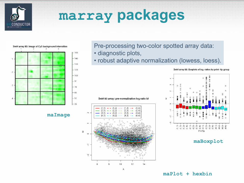
marray packages

Pre-processing two-color spotted array data:• diagnostic plots,• robust adaptive normalization (lowess, loess).

maPlot + hexbin

maBoxplot

maImage

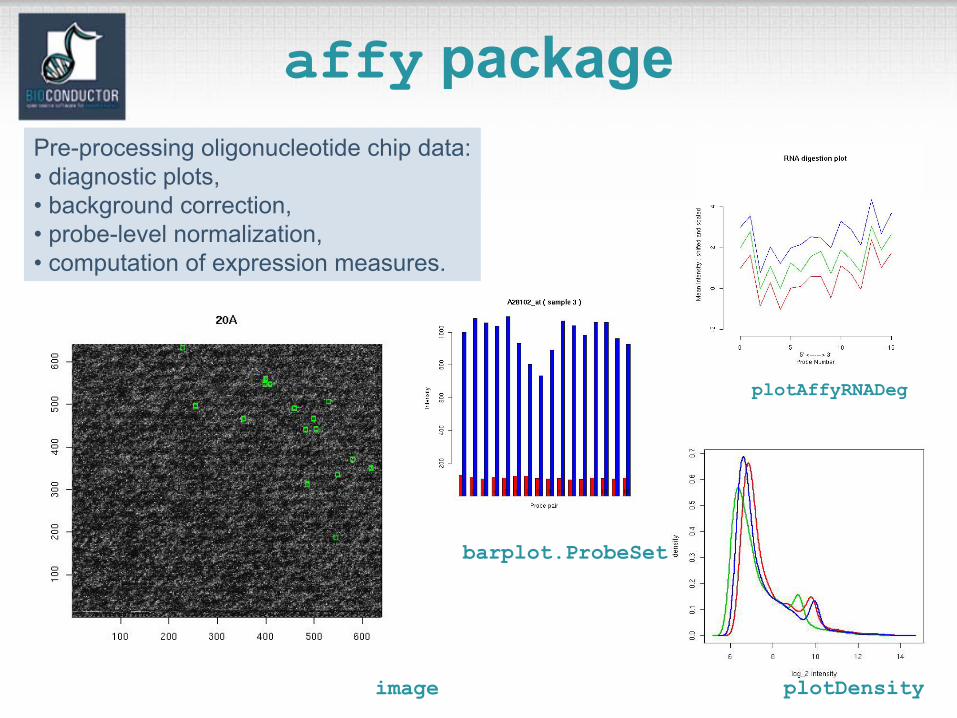
affy packagePre-processing oligonucleotide chip data:• diagnostic plots, • background correction, • probe-level normalization,• computation of expression measures.

image plotDensity

plotAffyRNADeg

barplot.ProbeSet

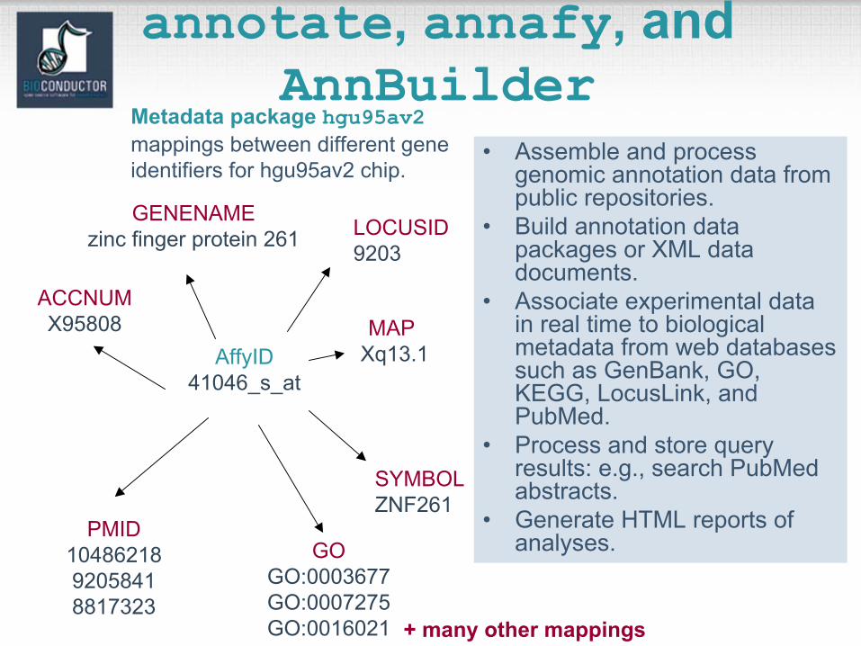
annotate, annafy, andAnnBuilder

• Assemble and process genomic annotation data from public repositories.

• Build annotation data packages or XML data documents.

• Associate experimental data in real time to biological metadata from web databases such as GenBank, GO, KEGG, LocusLink, and PubMed.

• Process and store query results: e.g., search PubMedabstracts.

• Generate HTML reports of analyses.

AffyID41046_s_at

ACCNUMX95808

LOCUSID9203

SYMBOLZNF261

GENENAMEzinc finger protein 261

MAP Xq13.1

PMID1048621892058418817323

GOGO:0003677GO:0007275GO:0016021 + many other mappings

Metadata package hgu95av2mappings between different gene identifiers for hgu95av2 chip.

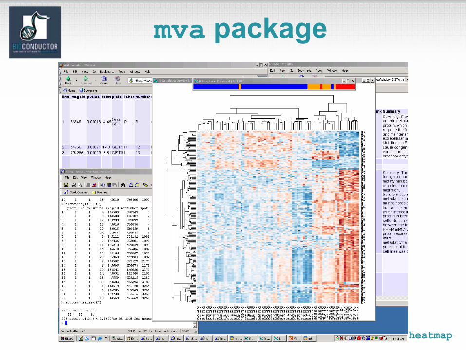
heatmap

mva package

Data complexity• Dimensionality.• Dynamic/evolving data: e.g., gene annotation,

sequence, literature.• Multiple data sources and locations: in-house,

WWW.• Multiple data types: numeric, textual, graphical.

No longer Xnxp!

We distinguish between biological metadata and experimental metadata.

Experimental metadata• Gene expression measures

– scanned images, i.e., raw data;– image quantitation data, i.e., output from image analysis;– normalized expression measures, i.e., log ratios or Affy

expression measures.• Reliability/quality information for the expression

measures.• Information on the probe sequences printed on the

arrays (array layout).• Information on the target samples hybridized to the

arrays.• See Minimum Information About a Microarray

Experiment (MIAME) standards and new MAGEMLpackage.

Biological metadata• Biological attributes that can be applied to the

experimental data. • E.g. for genes

– chromosomal location;– gene annotation (LocusLink, GO);– relevant literature (PubMed).

• Biological metadata sets are large, evolving rapidly, and typically distributed via the WWW.

• Tools: annotate, annaffy, and AnnBuilderpackages, and annotation data packages.

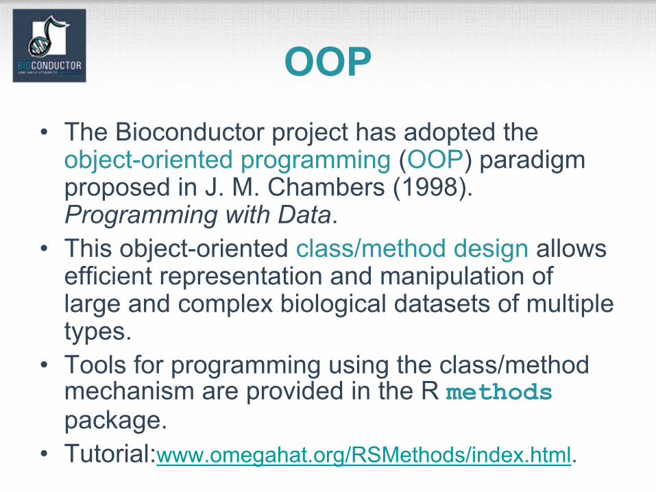
OOP• The Bioconductor project has adopted the

object-oriented programming (OOP) paradigm proposed in J. M. Chambers (1998).Programming with Data.

• This object-oriented class/method design allows efficient representation and manipulation of large and complex biological datasets of multiple types.

• Tools for programming using the class/method mechanism are provided in the R methodspackage.

• Tutorial:www.omegahat.org/RSMethods/index.html.

OOP: classes• A class provides a software abstraction of

a real world object. It reflects how we think of certain objects and what information these objects should contain.

• Classes are defined in terms of slots which contain the relevant data.

• An object is an instance of a class.• A class defines the structure, inheritance,

and initialization of objects.

OOP: methods• A method is a function that performs an action

on data (objects). • Methods define how a particular function should

behave depending on the class of its arguments.• Methods allow computations to be adapted to

particular data types, i.e., classes.• A generic function is a dispatcher, it examines its

arguments and determines the appropriate method to invoke.

• Examples of generic functions in R include plot, summary, print.

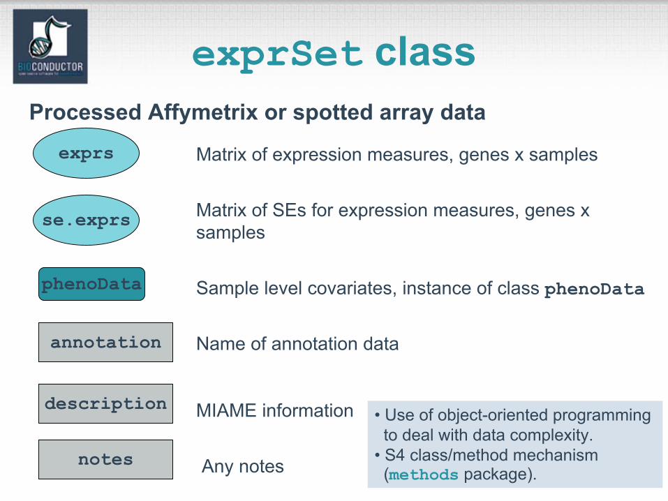
exprSet class

description

annotation

phenoData

Any notes

Matrix of expression measures, genes x samples

Matrix of SEs for expression measures, genes x samples

Sample level covariates, instance of class phenoData

Name of annotation data

MIAME information

se.exprs

exprs

notes

• Use of object-oriented programming to deal with data complexity.

• S4 class/method mechanism (methods package).

Processed Affymetrix or spotted array data

marrayRaw class

maRf

maW

maRb maGb

maGf

Pre-normalization intensity data for a batch of arrays

Matrix of red and green foreground intensities

Matrix of red and green background intensities

Matrix of spot quality weights

maNotes

maGnames

maTargets

maLayout Array layout parameters - marrayLayout

Description of spotted probe sequences- marrayInfoDescription of target samples - marrayInfo

Any notes

AffyBatch class

cdfName

exprs

nrow ncol

Probe-level intensity data for a batch of arrays (same CDF)

Dimensions of the array

Matrices of probe-level intensities and SEsrows probe cells, columns arrays.

Name of CDF file for arrays in the batch

se.exprs

description

annotation

phenoData

Any notes

Sample level covariates, instance of class phenoData

Name of annotation data

MIAME information

notes

Widgets• Widgets. Small-scale graphical user interfaces

(GUI), providing point & click access for specific tasks.

• E.g. File browsing and selection for data input, basic analyses.

• Packages: – tkWidgets: dataViewer, fileBrowser, fileWizard, importWizard, objectBrowser.

– widgetTools.

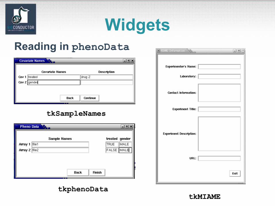
Widgets

tkMIAMEtkphenoData

tkSampleNames

Reading in phenoData

Getting Started

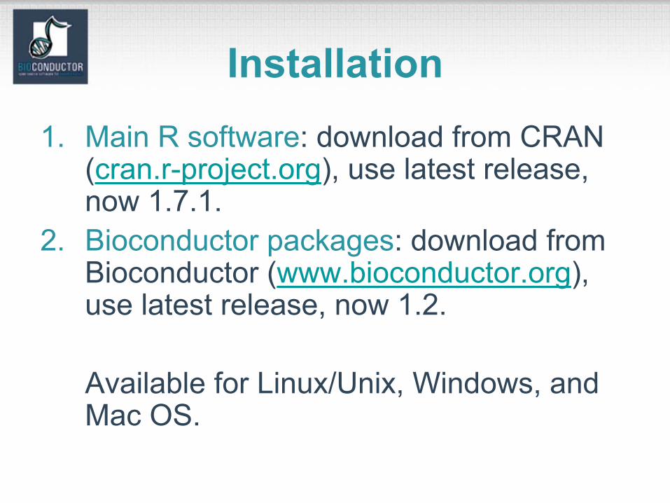
Installation1. Main R software: download from CRAN

(cran.r-project.org), use latest release, now 1.7.1.

2. Bioconductor packages: download from Bioconductor (www.bioconductor.org), use latest release, now 1.2.

Available for Linux/Unix, Windows, and Mac OS.

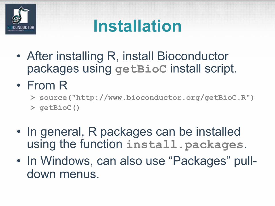
Installation• After installing R, install Bioconductor

packages using getBioC install script.• From R

> source("http://www.bioconductor.org/getBioC.R") > getBioC()

• In general, R packages can be installed using the function install.packages.

• In Windows, can also use “Packages” pull-down menus.

Installing vs. loading• Packages only need to be installed once .• But … packages must be loaded with each new

R session. • Packages are loaded using the function library. From R > library(Biobase)

or the “Packages” pull-down menus in Windows. • To update packages, use function update.packages or “Packages” pull-down menus in Windows.

• To quit: > q()

Documentation and help

• R manuals and tutorials:available from the R website or on-line in an R session.

• R on-line help system: detailed on-line documentation, available in text, HTML, PDF, and LaTeX formats.> help.start()> help(lm)> ?hclust> apropos(mean)> example(hclust)> demo()> demo(image)

Short courses

• Bioconductor short courses– modular training segments on software and

statistical methodology;– lectures notes, computer labs, and course

packages available on WWW for self-instruction.

Vignettes• Bioconductor has adopted a new documentation

paradigm, the vignette.• A vignette is an executable document consisting

of a collection of code chunks and documentation text chunks.

• Vignettes provide dynamic, integrated, and reproducible statistical documents that can be automatically updated if either data or analyses are changed.

• Vignettes can be generated using the Sweavefunction from the R tools package.

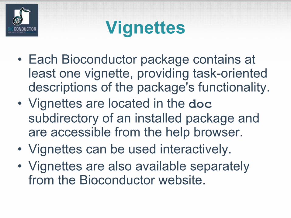
Vignettes• Each Bioconductor package contains at

least one vignette, providing task-oriented descriptions of the package's functionality.

• Vignettes are located in the doc subdirectory of an installed package and are accessible from the help browser.

• Vignettes can be used interactively.• Vignettes are also available separately

from the Bioconductor website.

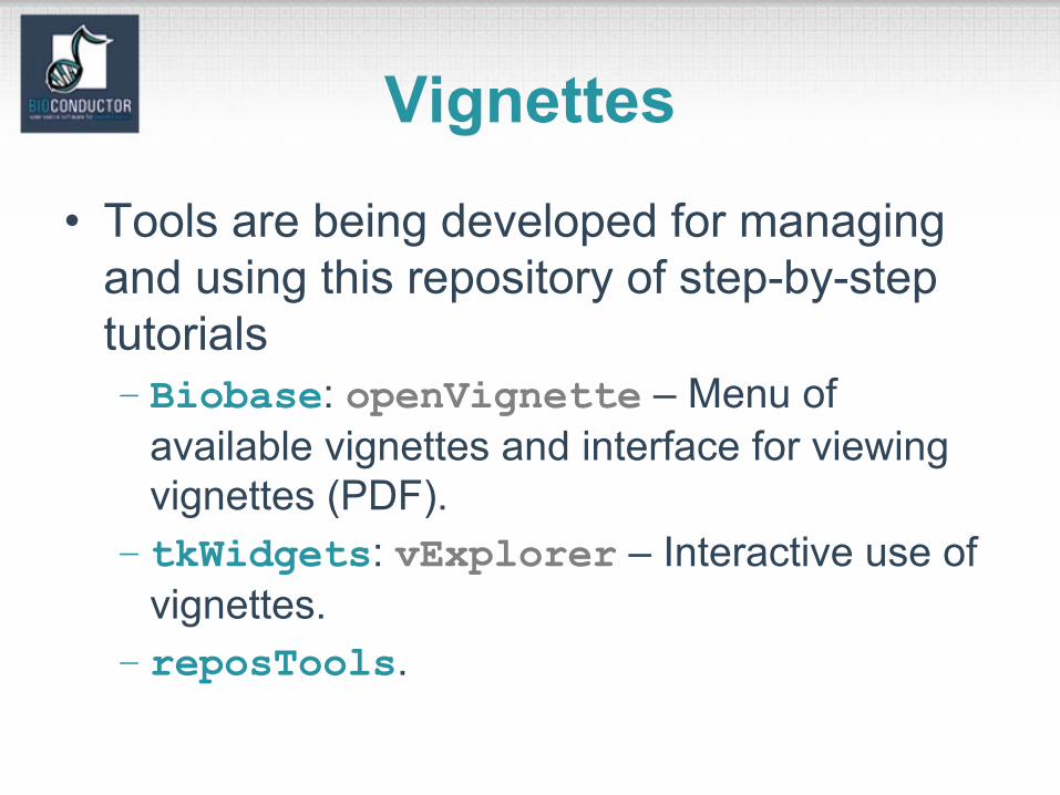
Vignettes• Tools are being developed for managing

and using this repository of step-by-step tutorials– Biobase: openVignette – Menu of

available vignettes and interface for viewing vignettes (PDF).

– tkWidgets: vExplorer – Interactive use of vignettes.

– reposTools.

Vignettes

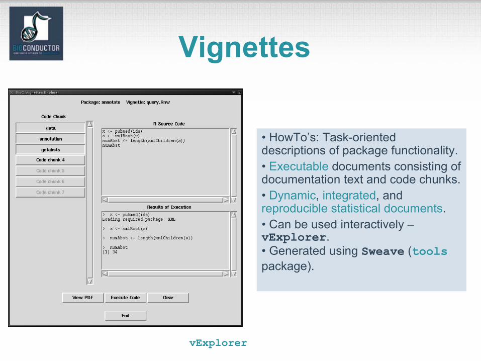
vExplorer

• HowTo’s: Task-oriented descriptions of package functionality.• Executable documents consisting of documentation text and code chunks.• Dynamic, integrated, and reproducible statistical documents.• Can be used interactively –vExplorer.• Generated using Sweave (toolspackage).

Sweave• The Sweave system allows the generation

of dynamic, integrated, and reproducible statistical documents intermixing text, code, and code output (textual and graphical).

• Functions are available in the R toolspackage.

• See ? Sweave and manualwww.ci.tuwien.ac.at/~leisch/Sweave/.

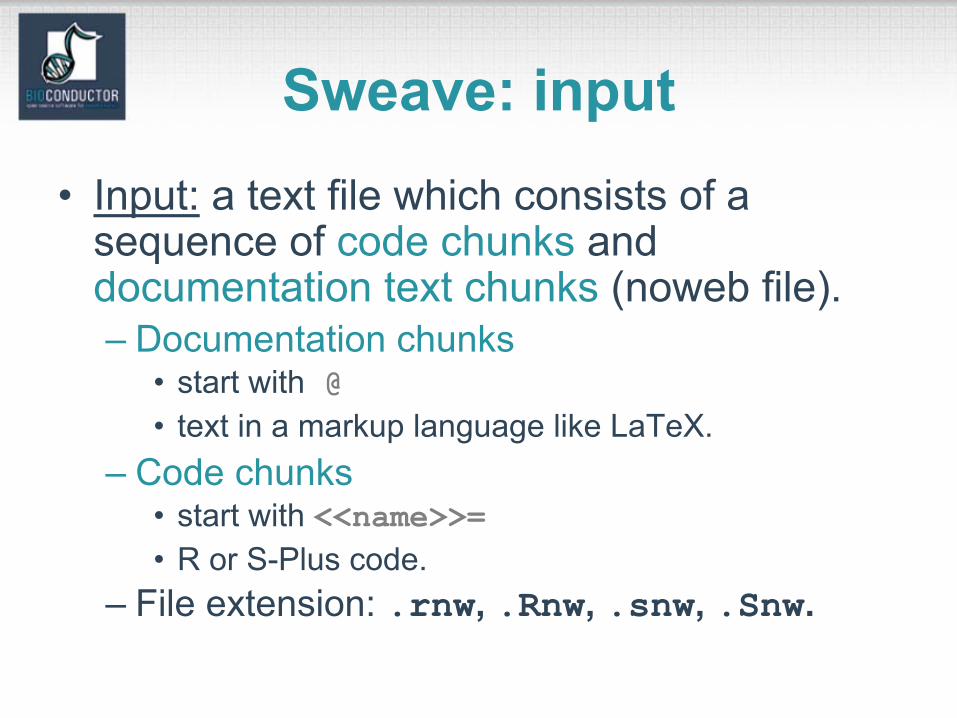
Sweave: input• Input: a text file which consists of a

sequence of code chunks and documentation text chunks (noweb file).– Documentation chunks

• start with @• text in a markup language like LaTeX.

– Code chunks• start with <<name>>=• R or S-Plus code.

– File extension: .rnw, .Rnw, .snw, .Snw.

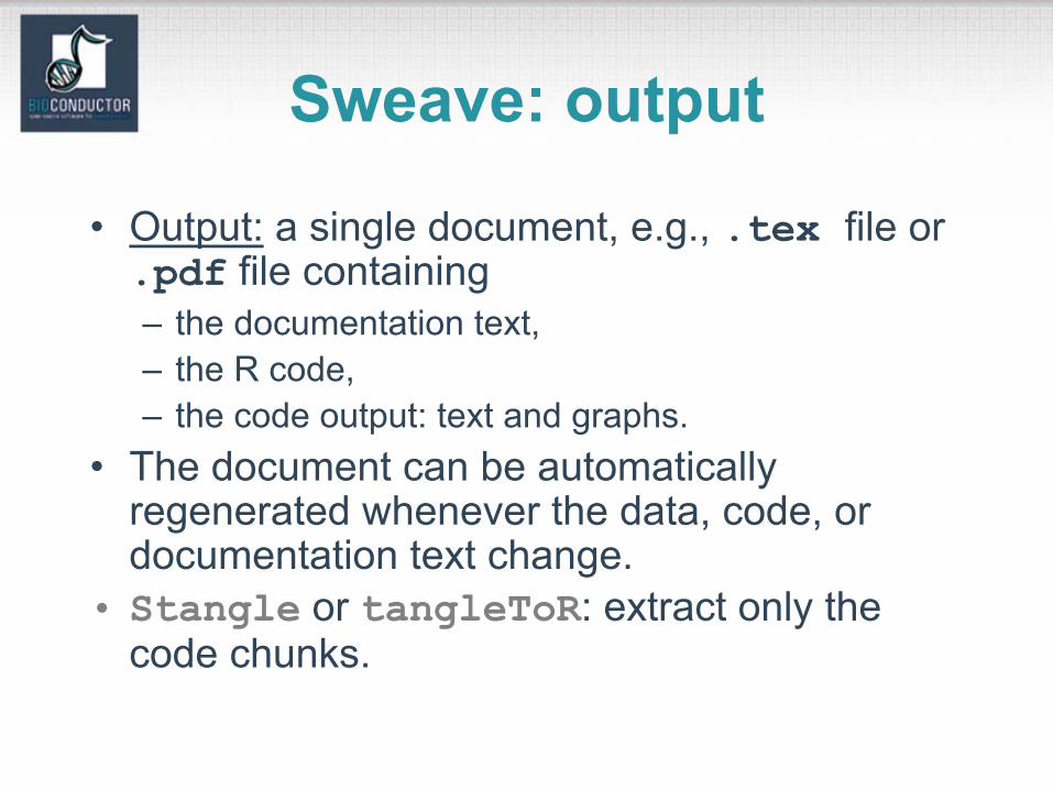
Sweave: output

• Output: a single document, e.g., .tex file or .pdf file containing– the documentation text,– the R code,– the code output: text and graphs.

• The document can be automatically regenerated whenever the data, code, or documentation text change.

• Stangle or tangleToR: extract only the code chunks.

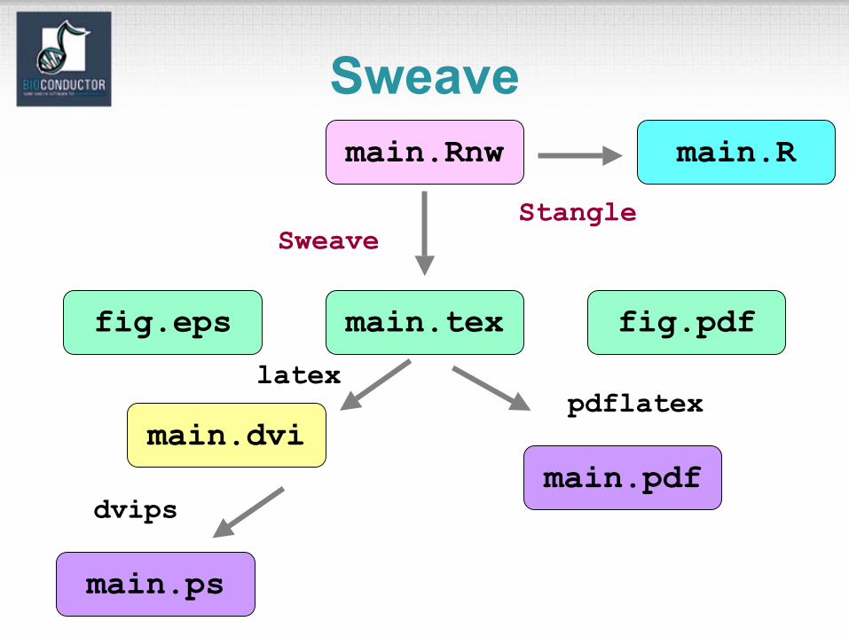
Sweavemain.Rnw

main.tex fig.pdffig.eps

main.dvi

main.ps

main.pdf

Sweave

latex

dvips

pdflatex

Stangle

main.R

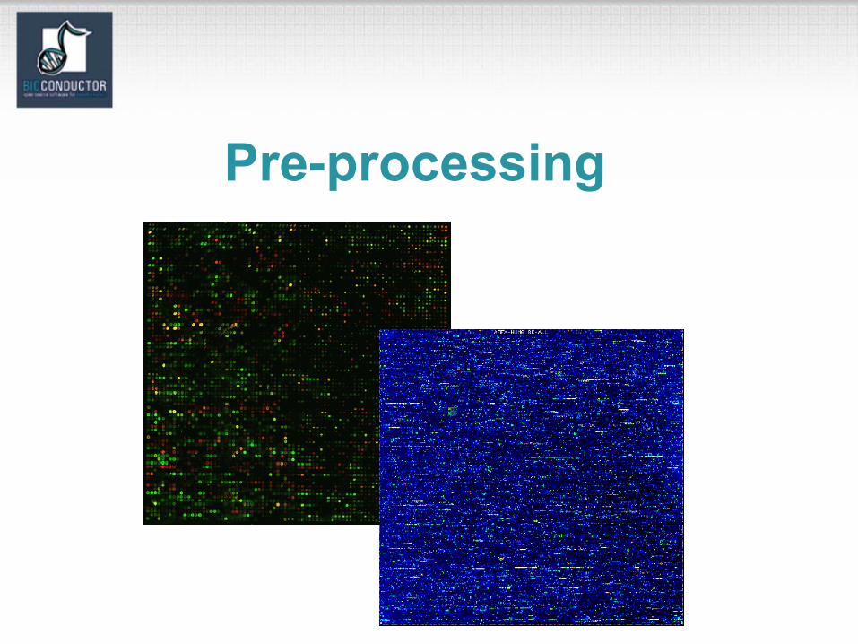
Pre-processing

Pre-processing packages

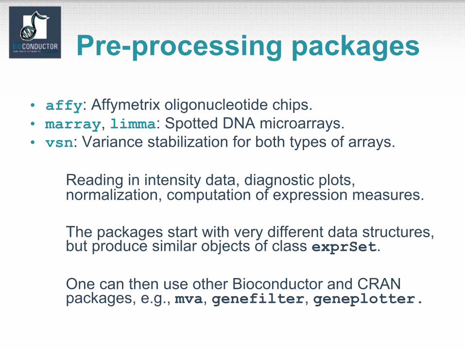
• affy: Affymetrix oligonucleotide chips.• marray, limma: Spotted DNA microarrays.• vsn: Variance stabilization for both types of arrays.

Reading in intensity data, diagnostic plots, normalization, computation of expression measures.

The packages start with very different data structures, but produce similar objects of class exprSet.

One can then use other Bioconductor and CRAN packages, e.g., mva, genefilter, geneplotter.

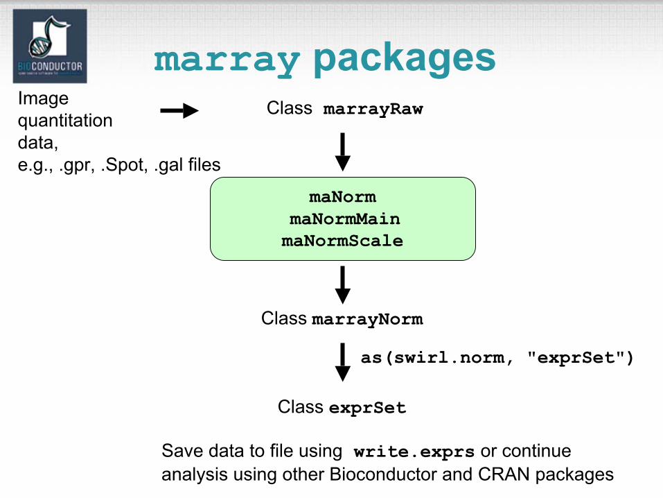
marray packages

maNormmaNormMainmaNormScale

Class marrayRaw

Class marrayNorm

Class exprSet

as(swirl.norm, "exprSet")

Save data to file using write.exprs or continue analysis using other Bioconductor and CRAN packages

Imagequantitationdata,e.g., .gpr, .Spot, .gal files

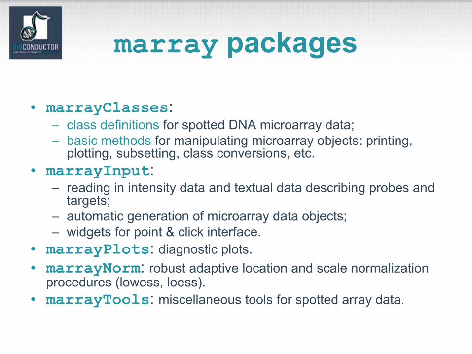
marray packages

• marrayClasses: – class definitions for spotted DNA microarray data;– basic methods for manipulating microarray objects: printing,

plotting, subsetting, class conversions, etc.• marrayInput:

– reading in intensity data and textual data describing probes andtargets;

– automatic generation of microarray data objects;– widgets for point & click interface.

• marrayPlots: diagnostic plots.• marrayNorm: robust adaptive location and scale normalization

procedures (lowess, loess).• marrayTools: miscellaneous tools for spotted array data.

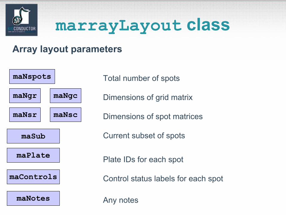
marrayLayout class

maNspots

maNgr maNgc

maNsr maNsc

maSub

maPlate

maControls

maNotes

Array layout parameters

Total number of spots

Dimensions of spot matrices

Dimensions of grid matrix

Current subset of spots

Plate IDs for each spot

Control status labels for each spot

Any notes

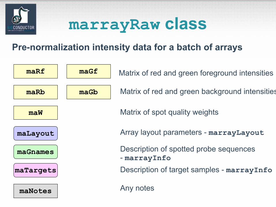
marrayRaw class

maRf

maW

maRb maGb

maGf

Pre-normalization intensity data for a batch of arrays

Matrix of red and green foreground intensities

Matrix of red and green background intensities

Matrix of spot quality weights

maNotes

maGnames

maTargets

maLayout Array layout parameters - marrayLayout

Description of spotted probe sequences- marrayInfoDescription of target samples - marrayInfo

Any notes

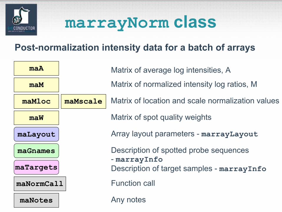
marrayNorm class

maA

maW

maMloc maMscale

maM

Post-normalization intensity data for a batch of arrays

Matrix of normalized intensity log ratios, M

Matrix of location and scale normalization values

Matrix of spot quality weights

maNotes

maGnames

maTargets

maLayout Array layout parameters - marrayLayout

Description of spotted probe sequences - marrayInfoDescription of target samples - marrayInfo

Any notes

Matrix of average log intensities, A

maNormCall Function call

marrayInput package

• marrayInput provides functions for reading microarray data into R and creating microarrayobjects of class marrayLayout, marrayInfo, and marrayRaw.

• Input– Image quantitation data, i.e., output files from

image analysis software.E.g. .gpr for GenePix, .spot for Spot.

– Textual description of probe sequences and target samples.E.g. gal files, god lists.

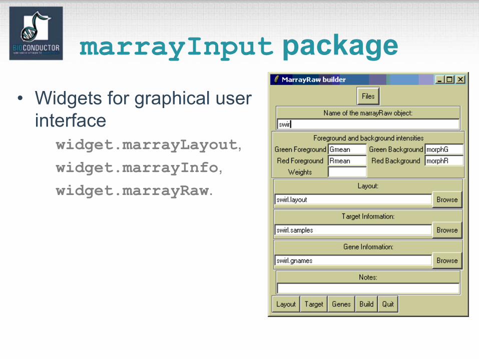
marrayInput package• Widgets for graphical user

interfacewidget.marrayLayout,widget.marrayInfo,widget.marrayRaw.

marrayPlots package• See demo(marrayPlots).• Diagnostic plots of spot statistics.

E.g. Red and green log intensities, intensity log ratios M, average log intensities A, spot area.– maImage: 2D spatial color images. – maBoxplot: boxplots.– maPlot: scatter-plots with fitted curves and

text highlighted. • Stratify plots according to layout

parameters such as print-tip-group, plate.E.g. MA-plots with loess fits by print-tip-group.

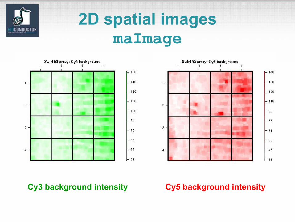
2D spatial imagesmaImage

Cy3 background intensity Cy5 background intensity

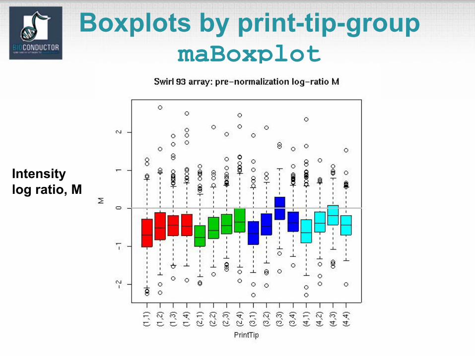
Boxplots by print-tip-groupmaBoxplot

Intensity log ratio, M

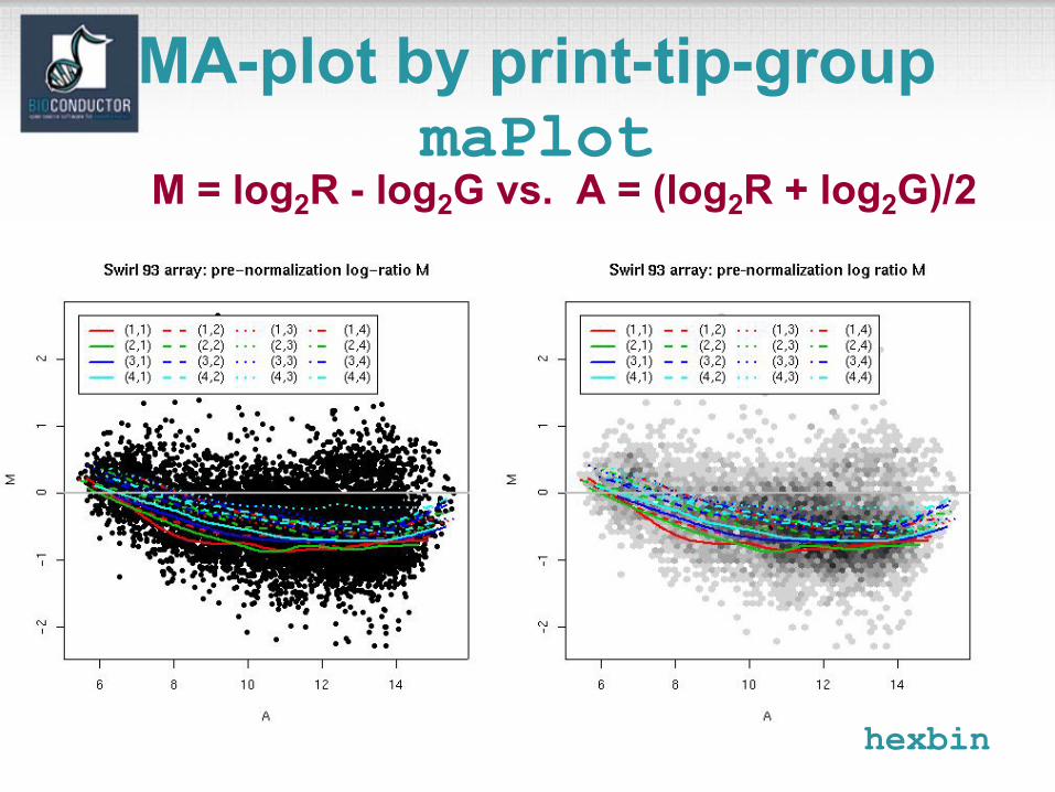
MA-plot by print-tip-groupmaPlot

M = log2R - log2G vs. A = (log2R + log2G)/2

hexbin

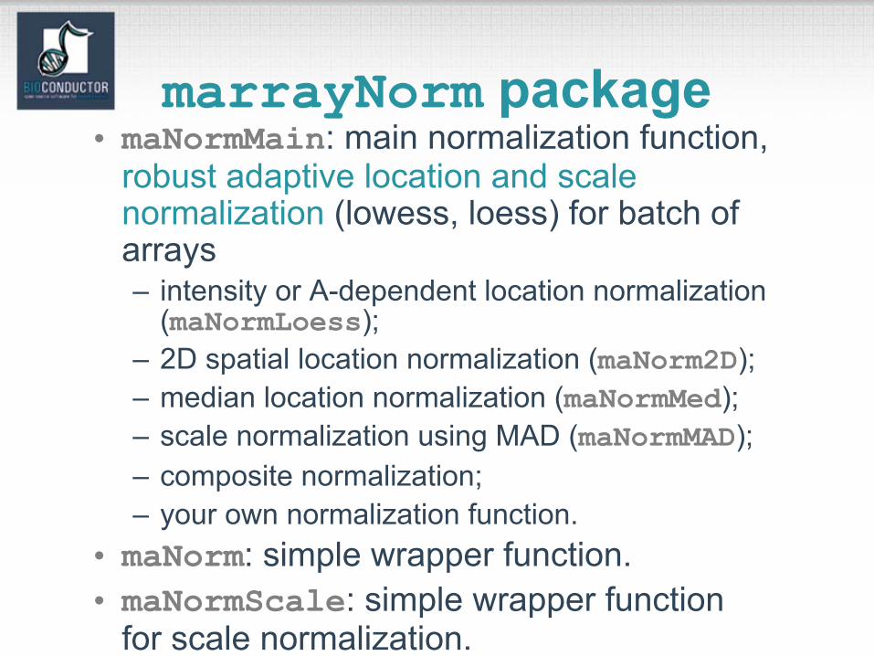
marrayNorm package• maNormMain: main normalization function,

robust adaptive location and scale normalization (lowess, loess) for batch of arrays– intensity or A-dependent location normalization

(maNormLoess);– 2D spatial location normalization (maNorm2D);– median location normalization (maNormMed);– scale normalization using MAD (maNormMAD);– composite normalization;– your own normalization function.

• maNorm: simple wrapper function.• maNormScale: simple wrapper function

for scale normalization.

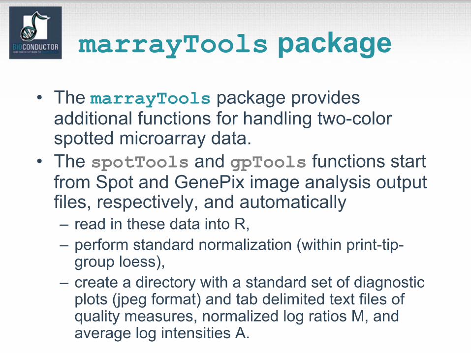
marrayTools package

• The marrayTools package provides additional functions for handling two-color spotted microarray data.

• The spotTools and gpTools functions start from Spot and GenePix image analysis output files, respectively, and automatically – read in these data into R, – perform standard normalization (within print-tip-

group loess), – create a directory with a standard set of diagnostic

plots (jpeg format) and tab delimited text files of quality measures, normalized log ratios M, and average log intensities A.

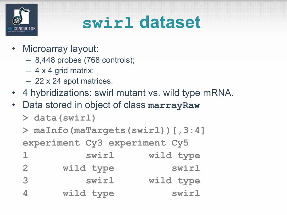
swirl dataset• Microarray layout:

– 8,448 probes (768 controls);– 4 x 4 grid matrix; – 22 x 24 spot matrices.

• 4 hybridizations: swirl mutant vs. wild type mRNA.• Data stored in object of class marrayRaw> data(swirl)> maInfo(maTargets(swirl))[,3:4]experiment Cy3 experiment Cy51 swirl wild type2 wild type swirl3 swirl wild type4 wild type swirl

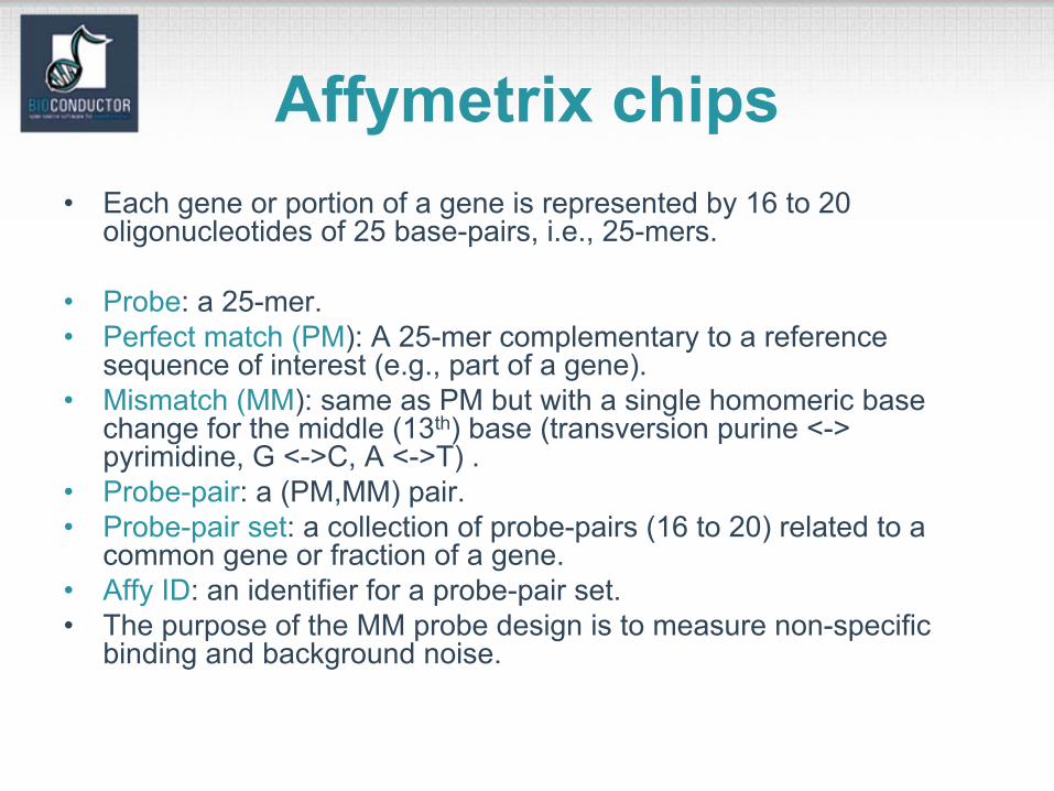
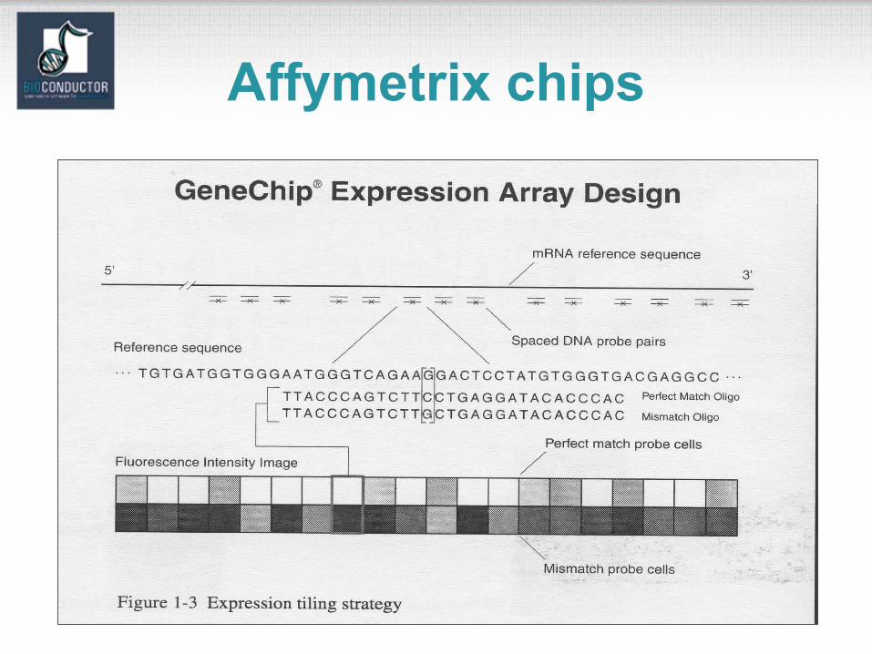
Affymetrix chips• Each gene or portion of a gene is represented by 16 to 20

oligonucleotides of 25 base-pairs, i.e., 25-mers.

• Probe: a 25-mer.• Perfect match (PM): A 25-mer complementary to a reference

sequence of interest (e.g., part of a gene).• Mismatch (MM): same as PM but with a single homomeric base

change for the middle (13th) base (transversion purine <-> pyrimidine, G <->C, A <->T) .

• Probe-pair: a (PM,MM) pair.• Probe-pair set: a collection of probe-pairs (16 to 20) related to a

common gene or fraction of a gene. • Affy ID: an identifier for a probe-pair set.• The purpose of the MM probe design is to measure non-specific

binding and background noise.

Affymetrix chips

Affymetrix chips

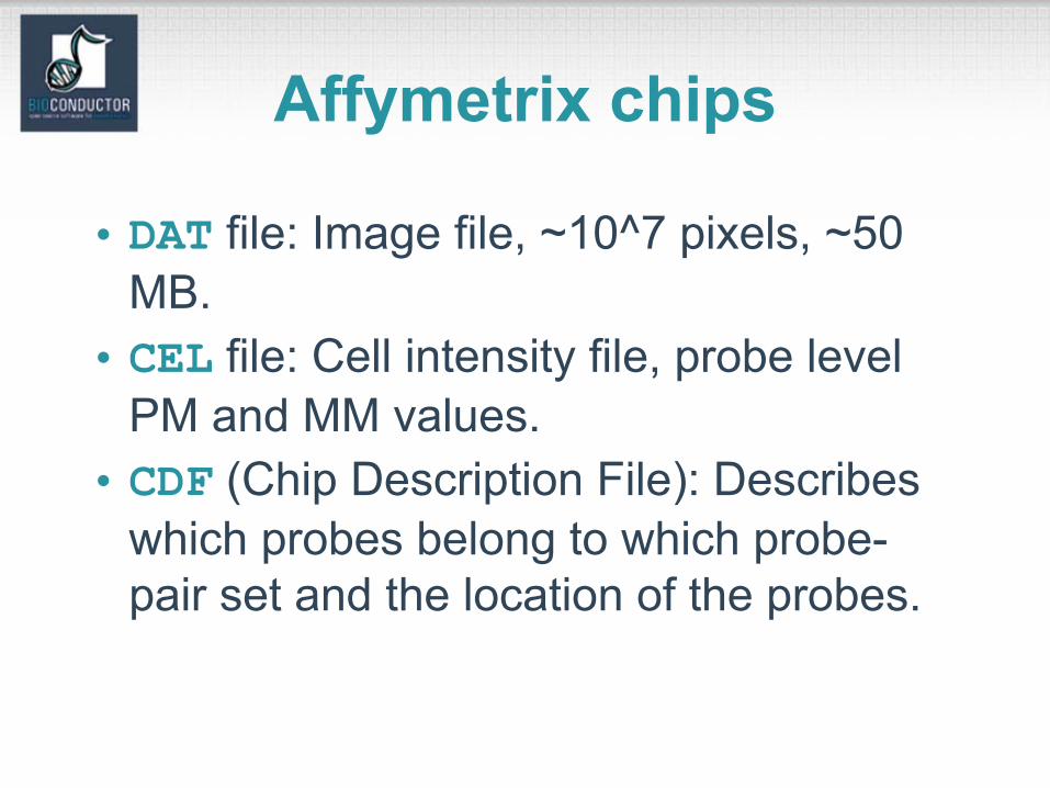
• DAT file: Image file, ~10^7 pixels, ~50 MB.

• CEL file: Cell intensity file, probe level PM and MM values.

• CDF (Chip Description File): Describes which probes belong to which probe-pair set and the location of the probes.

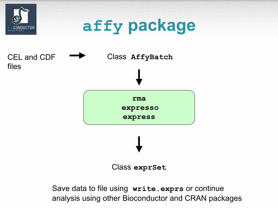
affy package

rmaexpressoexpress

Class AffyBatch

Class exprSet

Save data to file using write.exprs or continue analysis using other Bioconductor and CRAN packages

CEL and CDFfiles

affy package

• Class definitions for probe-level data: AffyBatch, ProbSet, Cdf, Cel.

• Basic methods for manipulating microarrayobjects: printing, plotting, subsetting.

• Functions and widgets for data input from CELand CDF files, and automatic generation of microarray data objects.

• Diagnostic plots: 2D spatial images, density plots, boxplots, MA-plots.

affy package

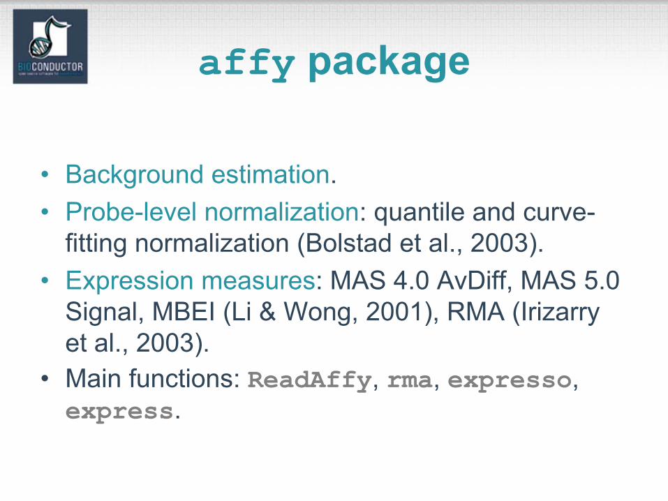
• Background estimation.• Probe-level normalization: quantile and curve-

fitting normalization (Bolstad et al., 2003).• Expression measures: MAS 4.0 AvDiff, MAS 5.0

Signal, MBEI (Li & Wong, 2001), RMA (Irizarry et al., 2003).

• Main functions: ReadAffy, rma, expresso, express.

AffyBatch class

cdfName

exprs

nrow ncol

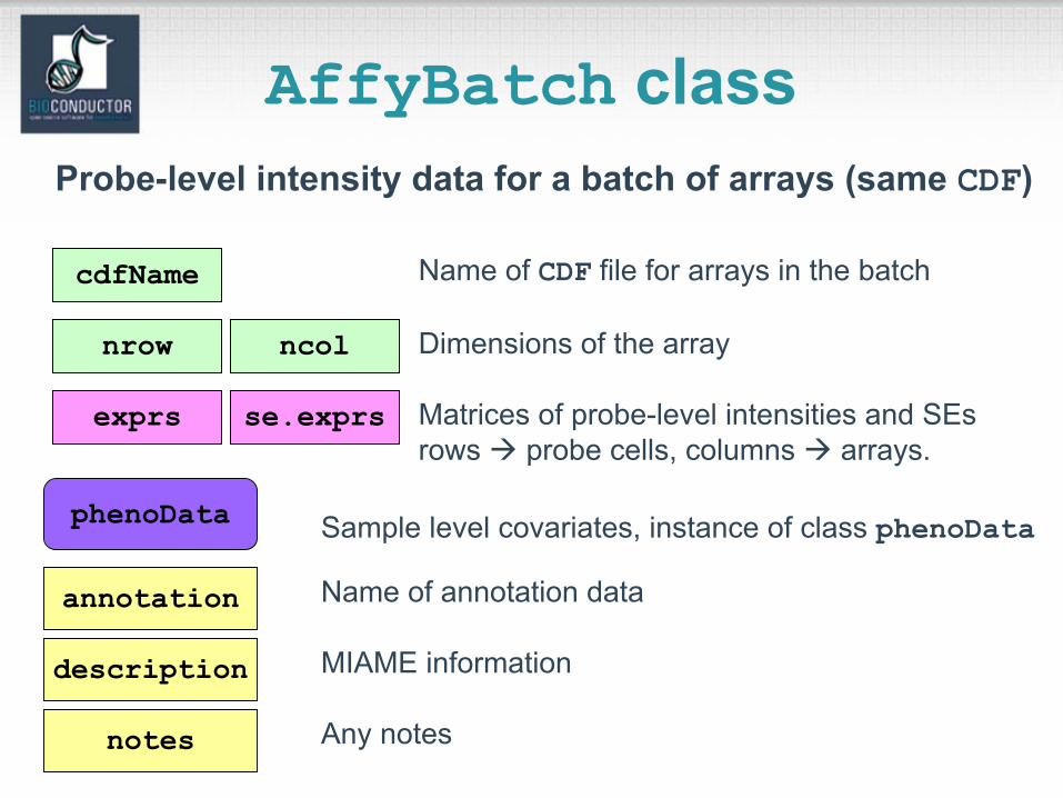
Probe-level intensity data for a batch of arrays (same CDF)

Dimensions of the array

Matrices of probe-level intensities and SEsrows probe cells, columns arrays.

Name of CDF file for arrays in the batch

se.exprs

description

annotation

phenoData

Any notes

Sample level covariates, instance of class phenoData

Name of annotation data

MIAME information

notes

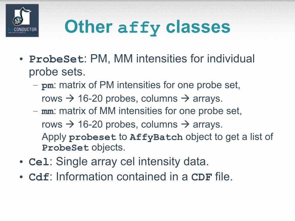
Other affy classes• ProbeSet: PM, MM intensities for individual

probe sets.– pm: matrix of PM intensities for one probe set,

rows 16-20 probes, columns arrays. – mm: matrix of MM intensities for one probe set,

rows 16-20 probes, columns arrays. Apply probeset to AffyBatch object to get a list of ProbeSet objects.

• Cel: Single array cel intensity data.• Cdf: Information contained in a CDF file.

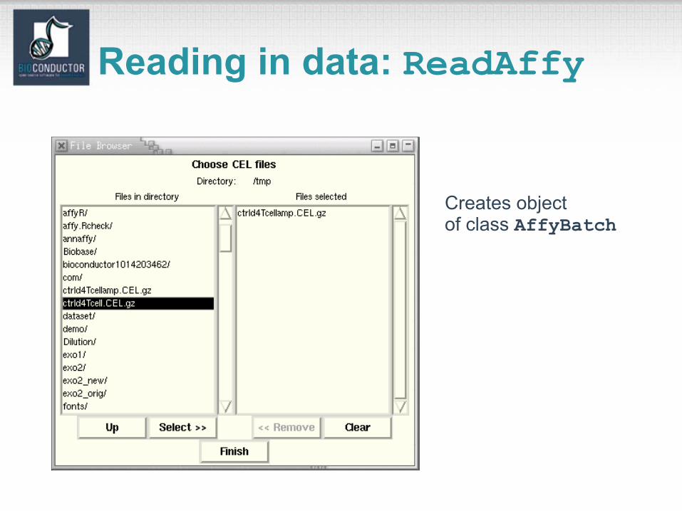
Reading in data: ReadAffy

Creates object of class AffyBatch

Accessing PM/MM data• probeNames: method for accessing

AffyIDs corresponding to individual probes.

• pm, mm: methods for accessing probe-level PM and MM intensities probes x arrays matrix.

• Can use on AffyBatch objects.

Diagnostic plots• See demo(affy).• Diagnostic plots of probe-level intensities, PM

and MM.– image: 2D spatial color images of log intensities

(AffyBatch, Cel).– boxplot: boxplots of log intensities

(AffyBatch).– mva.pairs: scatter-plots with fitted curves (apply exprs, pm, or mm to AffyBatch object).

– hist: density plots of log intensities (AffyBatch).

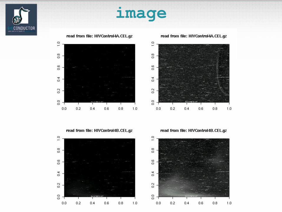
image

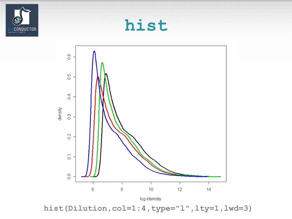
hist

hist(Dilution,col=1:4,type="l",lty=1,lwd=3)

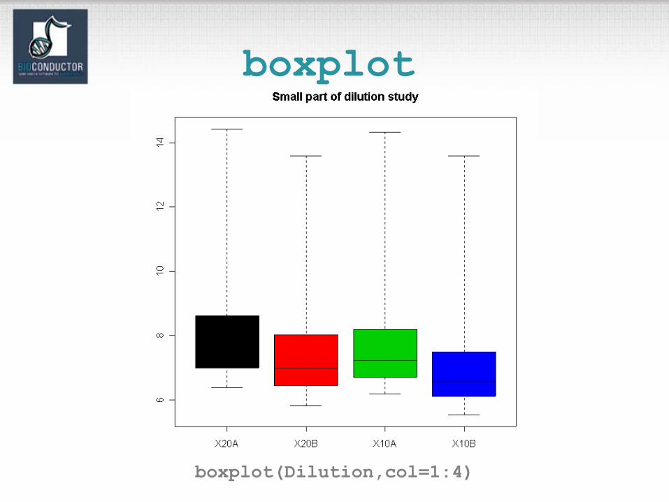
boxplot

boxplot(Dilution,col=1:4)

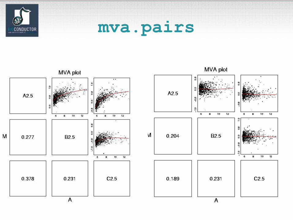
mva.pairs

Expression measures• expresso: Choice of common methods for

– background correction: bgcorrect.methods– normalization: normalize.AffyBatch.methods– probe specific corrections: pmcorrect.methods– expression measures: express.summary.stat.methods.

• rma: Fast implementation of RMA (Irizarry et al., 2003): model-based background correction, quantilenormalization, median polish expression measures.

• express: Implementing your own methods for computing expression measures.

• normalize: Normalization procedures in normalize.AffyBatch.methods or normalize.methods(object).

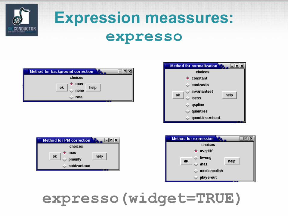
Expression meassures: expresso

expresso(widget=TRUE)

Probe sequence analysis• Examine probe intensities based on

location relative to 5’ end of the RNA sequence of interest.

• Expect probe intensities to be lower at 5’ end compared to 3’ end of mRNA.

• E.g.deg <- AffyRNAdeg(Dilution)plotAffyRNAdeg(deg)

CDF data packages• Data packages containing CDF information are

available at www.bioconductor.org.• Packages contain environment objects, which

provide mappings between AffyIDs and matrices of probe locations,

rows probe-pairs, columns PM, MM(e.g., 20X2 matrix for hu6800).

• cdfName slot of AffyBatch.• makecdfenv package.

Other packages• affycomp: assessment of Affymetrix

expression measures.• affydata: sample Affymetrix datasets.• annaffy: annotation functions. • gcrma: background adjustment using

sequence information.• makecdfenv: creating CDF environments

and packages.

Differential Gene Expression

Combining data across arrays

Genes

Arrays

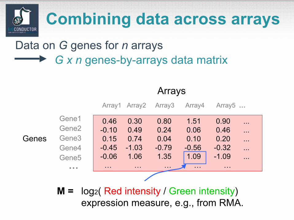
M = log2( Red intensity / Green intensity)expression measure, e.g., from RMA.

0.46 0.30 0.80 1.51 0.90 ...-0.10 0.49 0.24 0.06 0.46 ...0.15 0.74 0.04 0.10 0.20 ...-0.45 -1.03 -0.79 -0.56 -0.32 ...-0.06 1.06 1.35 1.09 -1.09 ...… … … … …

Data on G genes for n arrays

Array1 Array2 Array3 Array4 Array5 …

Gene2Gene1

Gene3

Gene5Gene4

G x n genes-by-arrays data matrix

…

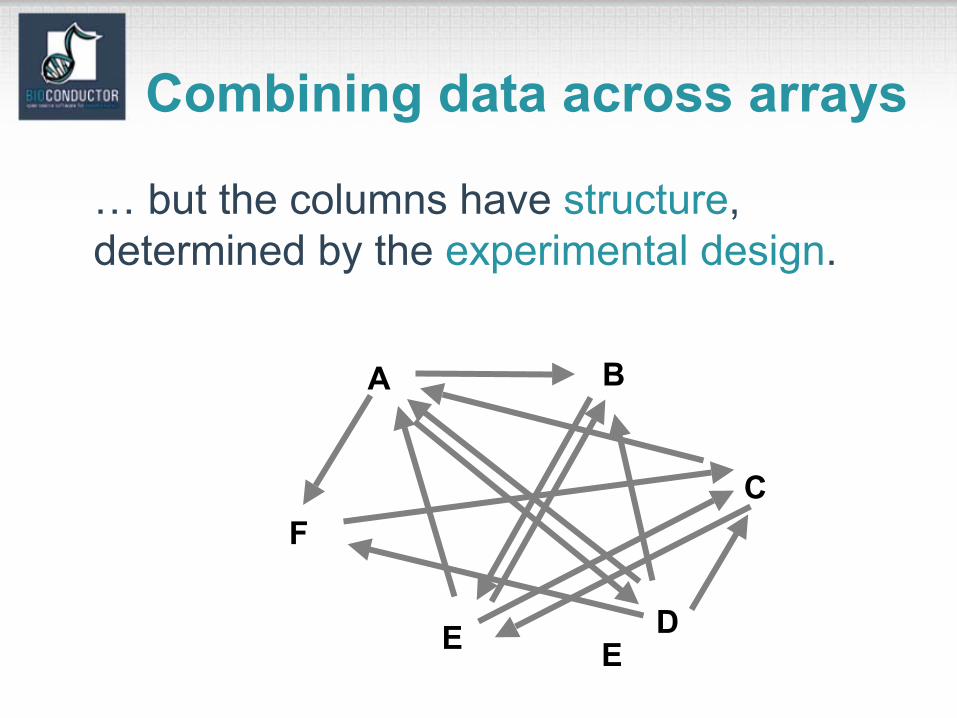
Combining data across arrays

… but the columns have structure, determined by the experimental design.

ED

F

BA

C

E

Combining data across arrays

• Spotted array factorial experiment. Each column corresponds to a pair of mRNA samples with different drug x dose x time combinations.

• Clinical trial. Each column corresponds to a patient, with associated clinical outcomes, such as survival and response to treatment.

• Linear models and extensions thereof can be used to effectively combine data across arrays for complex experimental designs.

Gene filtering• A very common task in microarray data analysis

is gene-by-gene selection. • Filter genes based on

– data quality criteria, e.g., absolute intensity or variance;

– subject matter knowledge;– their ability to differentiate cases from controls;– their spatial or temporal expression patterns.

• Depending on the experimental design, some highly specialized filters may be required and applied sequentially.

Gene filtering• Clinical trial. Filter genes based on

association with survival, e.g., using a Cox model.

• Factorial experiment. Filter genes based on interaction between two treatments, e.g., using 2-way ANOVA.

• Time-course experiment. Filter genes based on periodicity of expression pattern, e.g., using Fourier transform.

• The genefilter package provides tools to sequentially apply filters to the rows (genes) of a matrix or of an exprSet object.

• There are two main functions, filterfun and genefilter, for assembling and applying the filters, respectively.

• Any number of functions for specific filtering tasks can be defined and supplied to filterfun. E.g. Cox model p-values, coefficient of variation.

genefilter package

genefilter:separation of tasks

1. Select/define functions for specific filtering tasks.

2. Assemble the filters using the filterfunfunction.

3. Apply the filters using the genefilterfunction a logical vector, where TRUEindicates genes that are retained.

4. Apply this vector to the exprSet object to obtain a microarray object corresponding to the subset of interesting genes.

genefilter: supplied filters

• kOverA – select genes for which k samples have expression measures larger than A.

• gapFilter – select genes with a large IQR or gap (jump) in expression measures across samples.

• ttest – select genes according to t-test nominal p-values.

• Anova – select genes according to ANOVA nominal p-values.

• coxfilter – select genes according to Cox model nominal p-values.

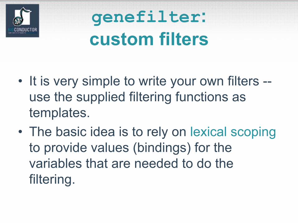
• It is very simple to write your own filters --use the supplied filtering functions as templates.

• The basic idea is to rely on lexical scopingto provide values (bindings) for the variables that are needed to do the filtering.

genefilter: custom filters

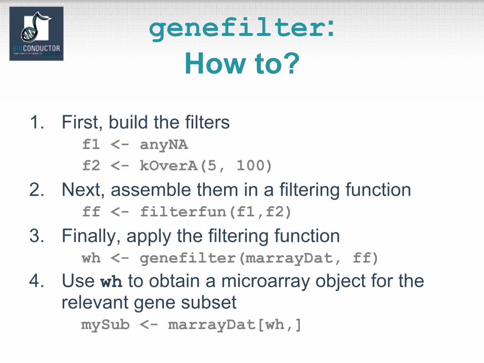
1. First, build the filtersf1 <- anyNAf2 <- kOverA(5, 100)

2. Next, assemble them in a filtering functionff <- filterfun(f1,f2)

3. Finally, apply the filtering functionwh <- genefilter(marrayDat, ff)

4. Use wh to obtain a microarray object for the relevant gene subset

mySub <- marrayDat[wh,]

genefilter: How to?

Differential expression

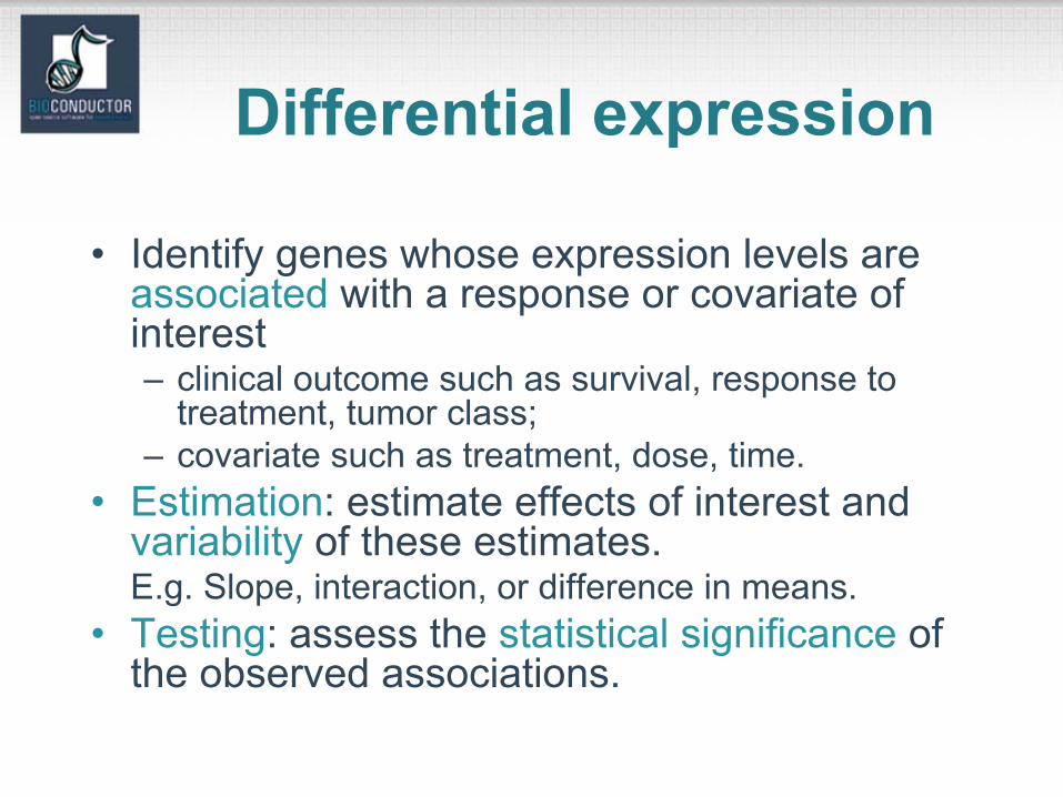
• Identify genes whose expression levels are associated with a response or covariate of interest– clinical outcome such as survival, response to

treatment, tumor class;– covariate such as treatment, dose, time.

• Estimation: estimate effects of interest and variability of these estimates. E.g. Slope, interaction, or difference in means.

• Testing: assess the statistical significance of the observed associations.

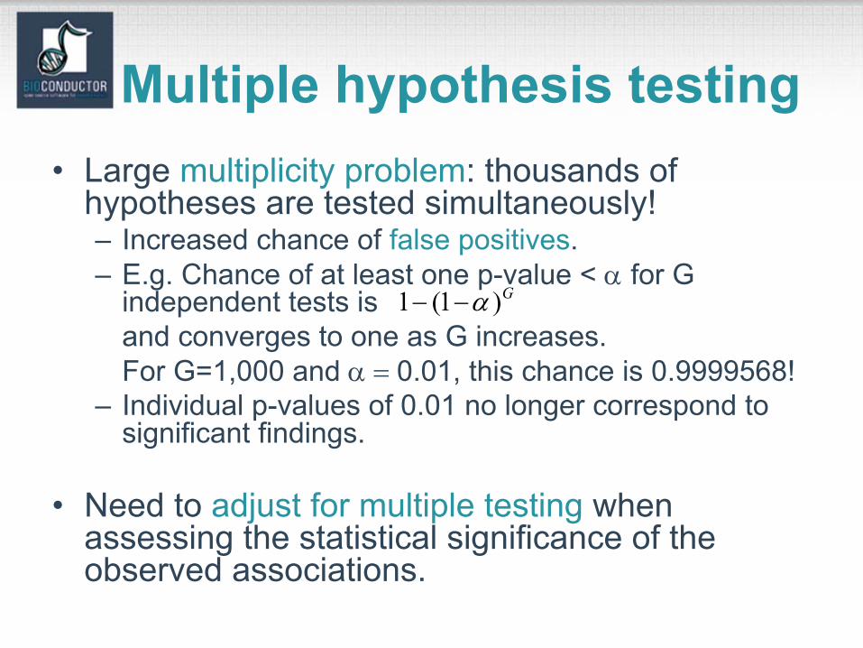
Multiple hypothesis testing• Large multiplicity problem: thousands of

hypotheses are tested simultaneously!– Increased chance of false positives. – E.g. Chance of at least one p-value < α for G

independent tests is and converges to one as G increases. For G=1,000 and α = 0.01, this chance is 0.9999568!

– Individual p-values of 0.01 no longer correspond to significant findings.

• Need to adjust for multiple testing when assessing the statistical significance of the observed associations.

G)−− α1(1

Multiple hypothesis testing • Define an appropriate Type I error or false

positive rate.• Apply multiple testing procedures that

– control this error rate under the true unknown data generating distribution,

– are powerful (few false negatives),– take into account the joint distribution of the test

statistics.• Report adjusted p-values for each gene which

reflect the overall Type I error rate for the experiment.

• Use resampling methods to deal with the unknown joint distribution of the test statistics.

multtest package

• Multiple testing procedures for controlling– Family-Wise Error Rate (FWER): Bonferroni, Holm (1979),

Hochberg (1986), Westfall & Young (1993) maxT and minP;– False Discovery Rate (FDR): Benjamini & Hochberg (1995),

Benjamini & Yekutieli (2001).• Tests based on t- or F-statistics for one- and two-factor

designs.• Permutation procedures for estimating adjusted p-

values. • Fast permutation algorithm for minP adjusted p-values.• Documentation: tutorial on multiple testing.

limma package• Fitting of gene-wise linear models to

estimate log ratios between two or more target samples simultaneously: lm.series, rlm.series, glm.series(handle replicate spots).

• ebayes: moderated t-statistics and log-odds of differential expression by empirical Bayes shrinkage of the standard errors towards a common value.

Distances, Prediction, and Cluster Analysis

Supervised vs. unsupervised learning

• Unsupervised learning a.k.a. cluster analysis– the classes are unknown a priori; – the goal is to discover these classes from the data.

• Supervised learning a.k.a. class prediction– the classes are predefined;– the goal is to understand the basis for the

classification from a set of labeled objects and to build a predictor for future unlabeled observations.

• Details in lectures from Dec. 2002 course at Fred Hutchinson Cancer Research Center.

Distances• Microarray data analysis often involves

– clustering genes and/or samples;– classifying genes and/or samples.

• Both types of analyses are based on a measure of distance (or similarity) between genes or samples.

• R has a number of functions for computing and plotting distance and similarity matrices.

Distances

• Distance functions– dist (mva): Euclidean, Manhattan, Canberra, binary;– daisy (cluster).

• Correlation functions– cor, cov.wt.

• Plotting functions– image;– plotcorr (ellipse);– plot.cor, plot.mat (sma).

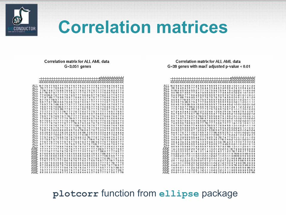
Correlation matrices

plotcorr function from ellipse package

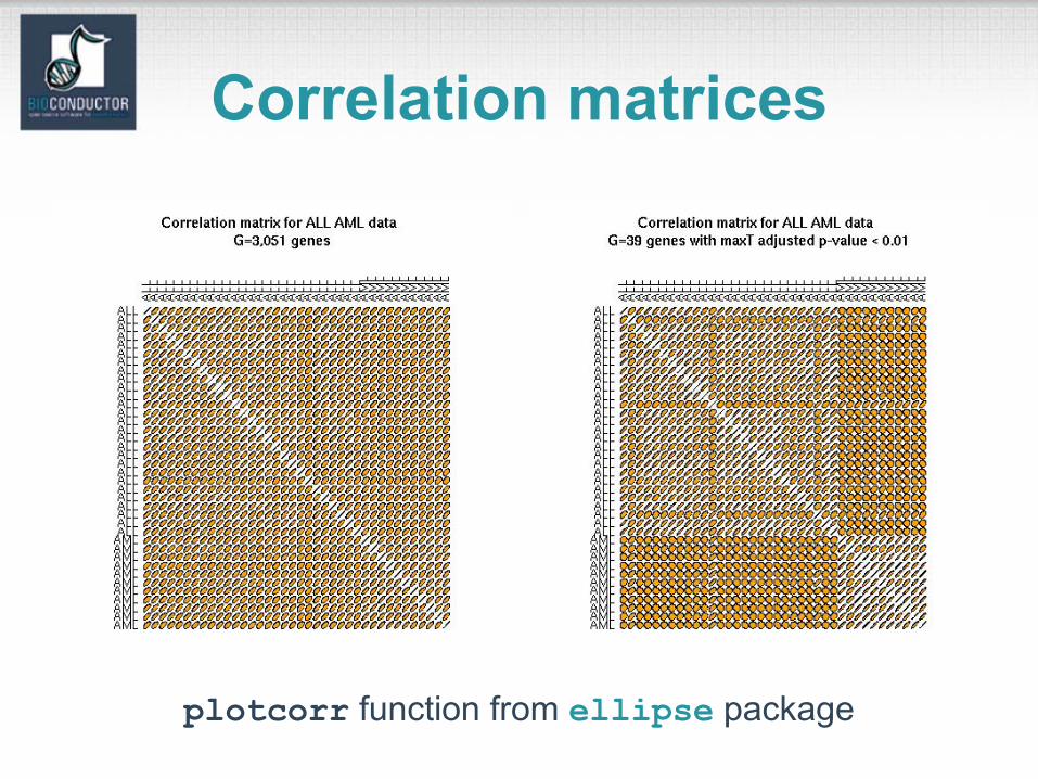
Correlation matrices

plotcorr function from ellipse package

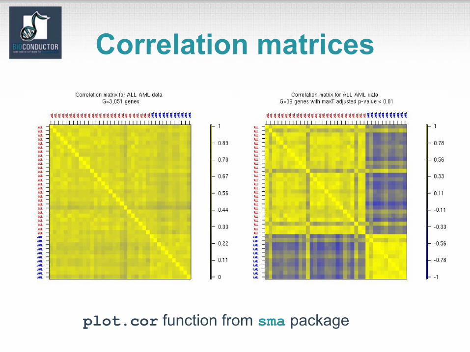
Correlation matrices

plot.cor function from sma package

Multidimensional scaling• Given any n x n distance matrix D,

multidimensional scaling (MDS) is concerned with identifying n points in Euclidean space with a similar distance structure D'.

• The purpose is to provide a lower dimensional representation of the distances which conveys information on the relationships between the nobjects, such as the existence of clusters or one-dimensional structure in the data (e.g., seriation).

MDS• There are different approaches for reducing

dimensionality, depending on how one defines similarity between the old and new distance matrices for the n objects, i.e., depending on the objective or stress function S that one seeks to minimize.– Least-squares scaling

– Sammon mapping places more emphasis on smaller dissimilarities (and hence should be preferred for clustering methods)

–– Shepard-Kruskal non-metric scaling is based on

ranks, i.e., the order of the distances is more important than their actual values.

( ) 2/12)'()',( ∑ −= ijij ddDDS

ijijij dddDDS /)'()',( 2∑ −=

MDS and PCA• When the distance matrix D is the Euclidean distance

matrix between the rows of an n x m matrix X, there is a duality between principal component analysis (PCA) and MDS.

• The k-dimensional classical solution to the MDS problem is given by the centered scores of the n objects on the first k principal components.

• The classical solution of MDS in k-dimensional space minimizes the sum of squared differences between the entries of the new and old distance matrices, i.e., is optimal for least-squares scaling.

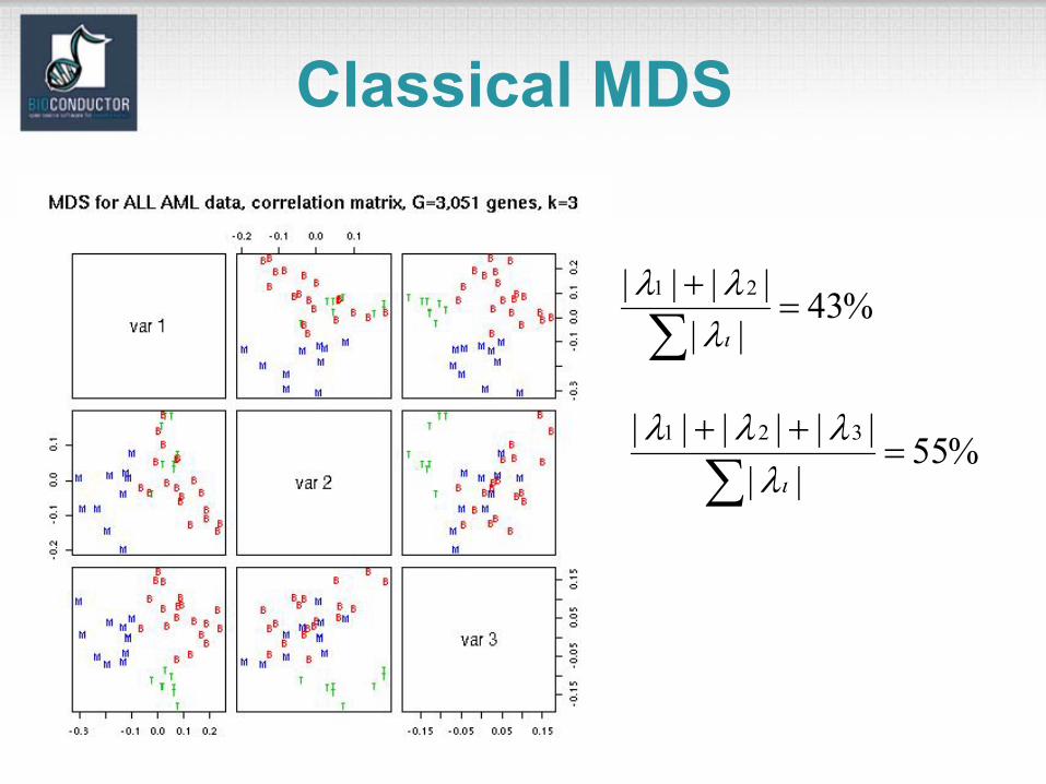
MDS• As with PCA, the quality of the

representation will depend on the magnitude of the first k eigenvalues.

• One should choose a value for k that is small enough for ease of representation, but also corresponds to a substantial “proportion of the distance matrix explained”.

MDS• N.B. The MDS solution reflects not only

the choice of a distance function, but also the features selected.

• If features (genes) are selected to separate the data into two groups (e.g., on the basis of two-sample t-statistics), it should come as no surprise that an MDS plot has two groups. In this instance, MDS is not a confirmatory approach.

R MDS software

• cmdscale: Classical solution to MDS, in package mva.

• sammon: Sammon mapping, in package MASS.

• isoMDS: Shepard-Kruskal's non-metric MDS, in package MASS.

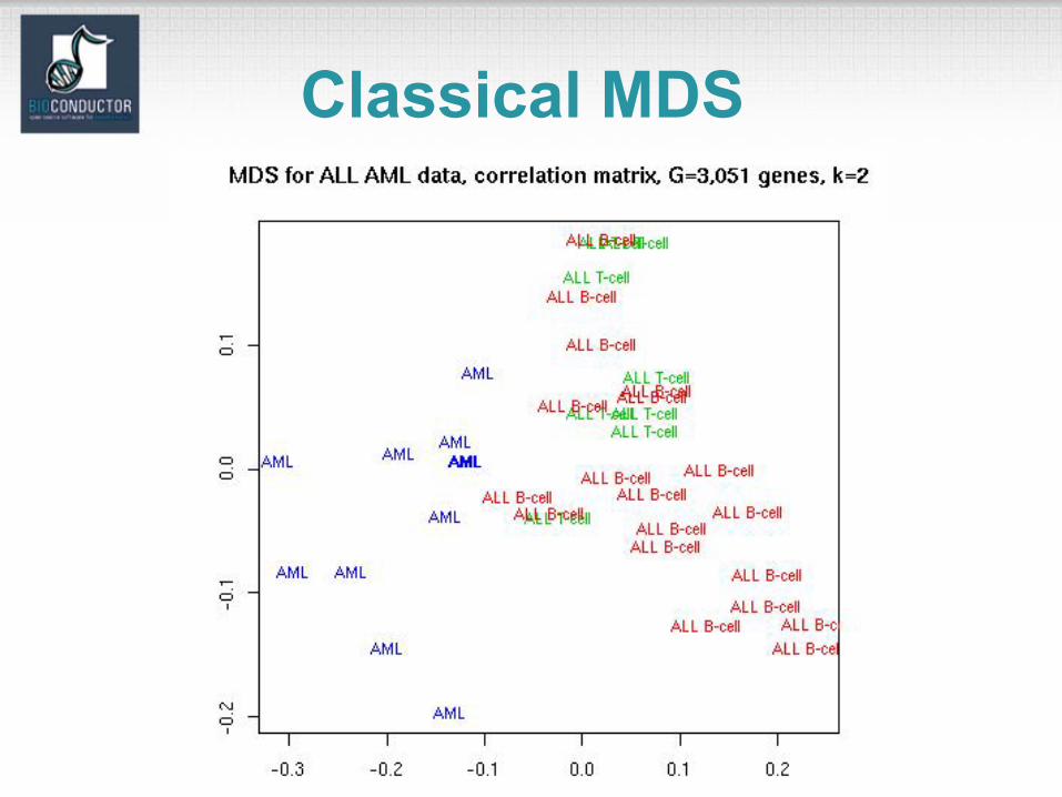
Classical MDS

Classical MDS

%43|||||| 2=

+

∑1

ιλλλ

%55||

|||||| 32=

++

∑1

ιλλλλ

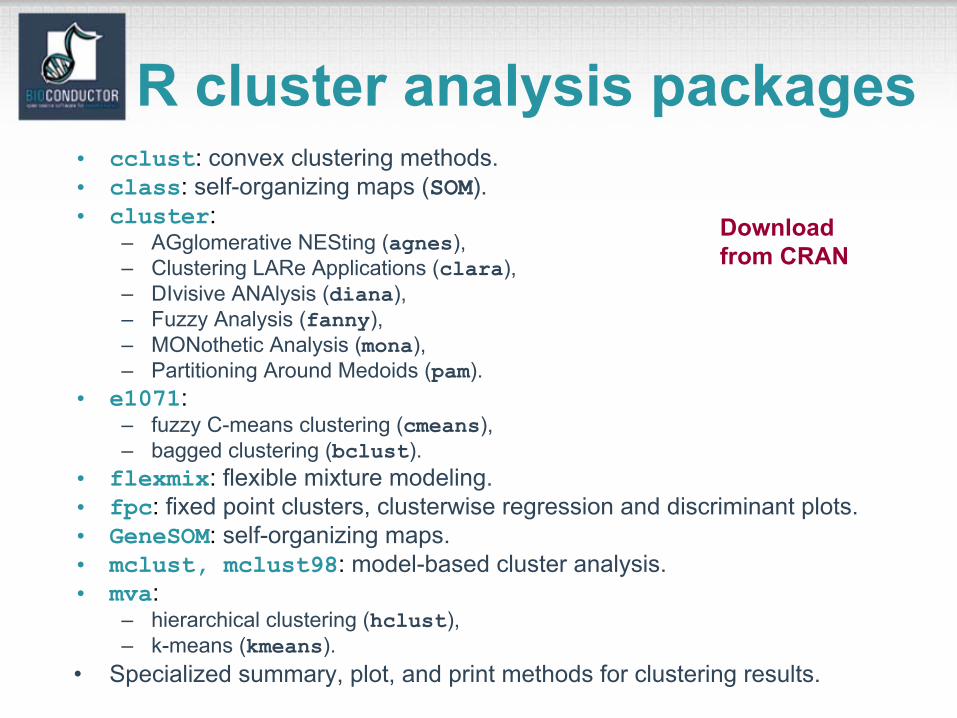
R cluster analysis packages• cclust: convex clustering methods.• class: self-organizing maps (SOM).• cluster:

– AGglomerative NESting (agnes), – Clustering LARe Applications (clara), – DIvisive ANAlysis (diana), – Fuzzy Analysis (fanny), – MONothetic Analysis (mona), – Partitioning Around Medoids (pam).

• e1071: – fuzzy C-means clustering (cmeans), – bagged clustering (bclust).

• flexmix: flexible mixture modeling. • fpc: fixed point clusters, clusterwise regression and discriminant plots.• GeneSOM: self-organizing maps.• mclust, mclust98: model-based cluster analysis.• mva:

– hierarchical clustering (hclust), – k-means (kmeans).

• Specialized summary, plot, and print methods for clustering results.

Downloadfrom CRAN

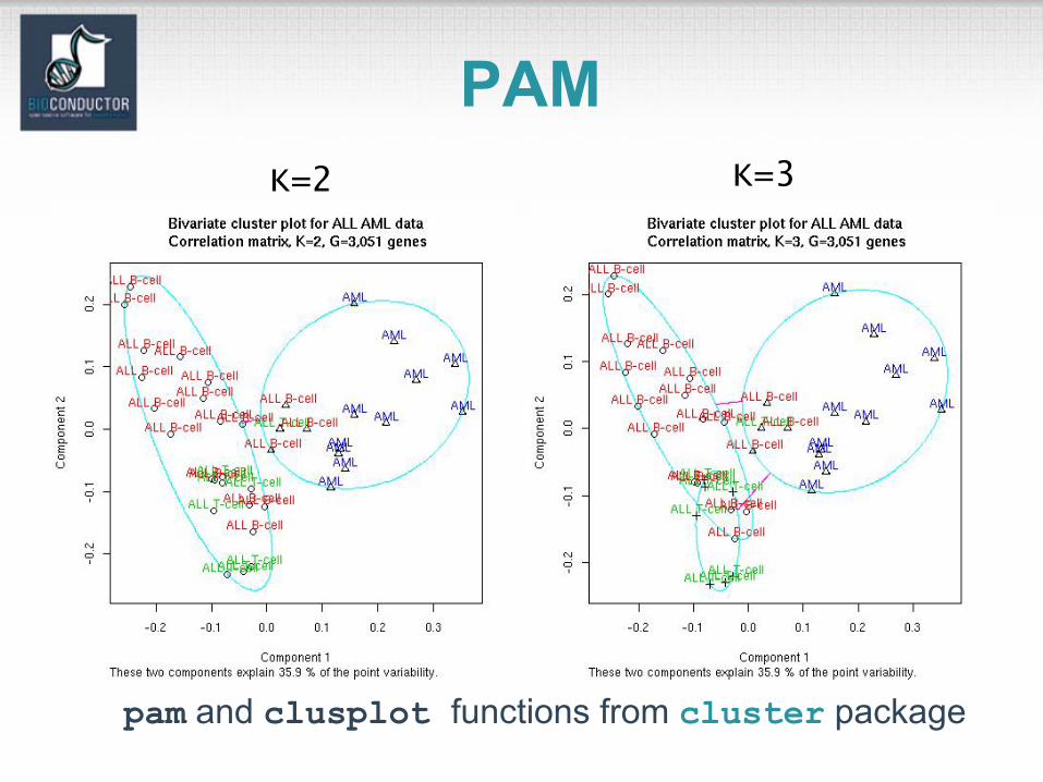
pam and clusplot functions from cluster package

PAMK=2 K=3

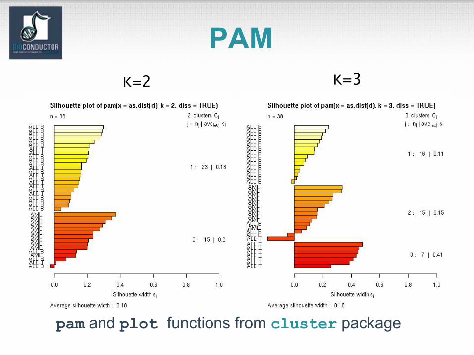
pam and plot functions from cluster package

PAMK=2 K=3

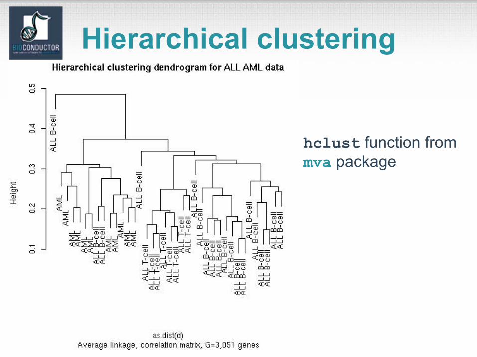
hclust function from mva package

Hierarchical clustering

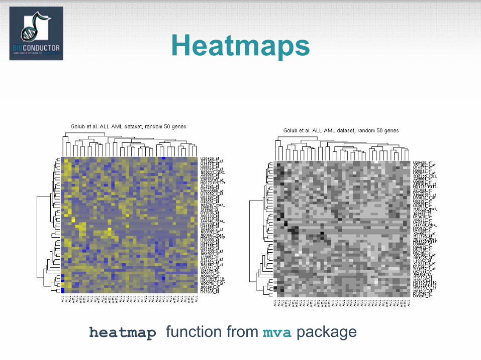
Heatmaps

heatmap function from mva package

Dendrograms• N.B. While dendrograms are appealing because

of their apparent ease of interpretation, they can be misleading.

• First, the dendrogram corresponding to a given hierarchical clustering is not unique, since for each merge one needs to specify which subtreeshould go on the left and which on the right ---there are 2^(n-1) choices.

• The default in the R function hclust is to order the subtrees so that the tighter cluster is on the left.

Dendrograms• Second, dendrograms impose structure on

the data, instead of revealing structure in these data.

• Such a representation will be valid only to the extent that the pairwise distances possess the hierarchical structure imposed by the clustering algorithm.

Dendrograms• The cophenetic correlation coefficient can be

used to measure how well the hierarchical structure from the dendrogram represents the actual distances.

• This measure is defined as the correlation between the n(n-1)/2 pairwise distances between observations and their copheneticdissimilarities, i.e., the between cluster distances at which two observations are first joined together in the same cluster.

• Function cophenetic in mva package.

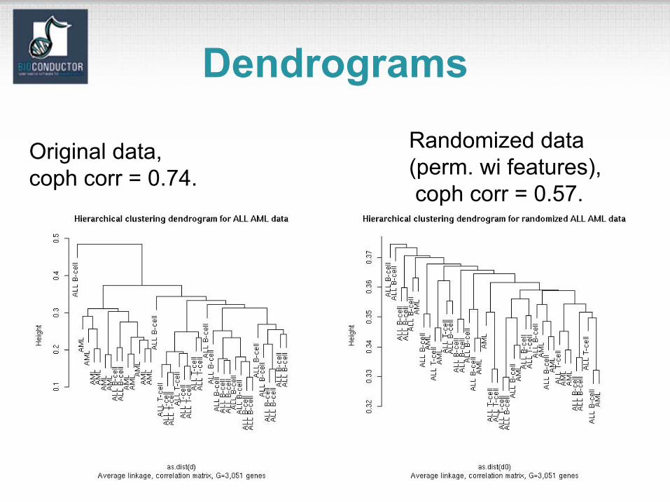
Dendrograms

Original data, coph corr = 0.74.

Randomized data (perm. wi features),coph corr = 0.57.

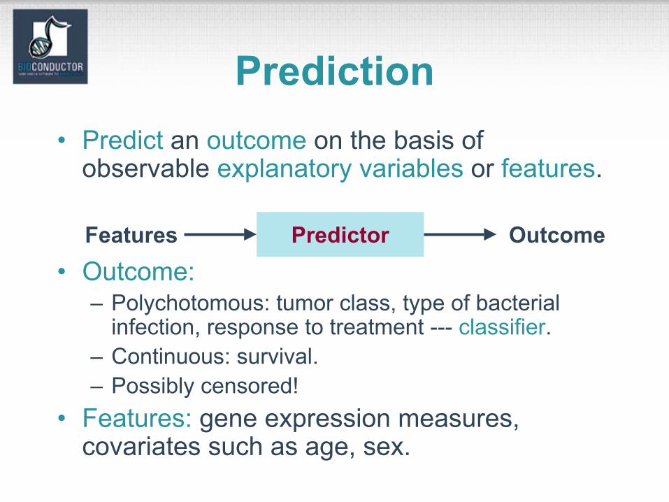
Prediction• Predict an outcome on the basis of

observable explanatory variables or features.

• Outcome:– Polychotomous: tumor class, type of bacterial

infection, response to treatment --- classifier.– Continuous: survival.– Possibly censored!

• Features: gene expression measures, covariates such as age, sex.

Predictor OutcomeFeatures

Class prediction• Old and extensive literature on class

prediction, in statistics and machine learning.• Examples of classifiers

– nearest neighbor classifiers (k-NN);– discriminant analysis: linear, quadratic, logistic;– neural networks;– classification trees;– support vector machines.

• Aggregated classifiers: bagging and boosting.• Comparison on microarray data:

simple classifiers like k-NN and naïve Bayesperform remarkably well.

R class prediction packages

• class: – k-nearest neighbor (knn), – learning vector quantization (lvq).

• classPP: projection pursuit.• e1071: support vector machines (svm).• ipred: bagging, resampling based estimation of prediction error.• knnTree: k-nn classification with variable selection inside leaves of a

tree.• LogitBoost: boosting for tree stumps.• MASS: linear and quadratic discriminant analysis (lda, qda). • mlbench: machine learning benchmark problems.• nnet: feed-forward neural networks and multinomial log-linear models.• pamR: prediction analysis for microarrays.• randomForest: random forests.• rpart: classification and regression trees.• sma: diagonal linear and quadratic discriminant analysis, naïve Bayes

(stat.diag.da).

Downloadfrom CRAN

Performance assessment• Classification error rates, or related

measures, are usually reported– to compare the performance of different

classifiers; – to support statements such as

“clinical outcome X for cancer Y can be predicted accurately based on gene expression measures”.

• Classification error rates can be estimated by resampling, e.g., bootstrap or cross-validation.

Performance assessment• It is essential to take into account feature

selection and other training decisions in the error rate estimation process.E.g. Number of neighbors in k-NN, kernel in SVMs.

• Otherwise, error estimates can be severely biased downward, i.e., overly optimistic.

Other important issues• Loss function;• Censoring;• Standardization;• Distance function;• Feature selection;• Class priors;• Binary vs. polychotomous classification.