Seediscussions,stats,andauthorprofilesforthispublicationat:https://www.researchgate.net/publication/257233676

SeparationoflargescalewaterstoragepatternsoverIranusingGRACE,altimetryandhydrologicaldata

ArticleinRemoteSensingofEnvironment·September2013

DOI:10.1016/j.rse.2013.09.025

CITATIONS

23

READS

384

8authors,including:

EhsanForootan

CardiffUniversity

82PUBLICATIONS403CITATIONS

SEEPROFILE

JürgenKusche

UniversityofBonn

198PUBLICATIONS1,962CITATIONS

SEEPROFILE

MohammadA.Sharifi

UniversityofTehran

139PUBLICATIONS432CITATIONS

SEEPROFILE

JosephAwange

CurtinUniversity

252PUBLICATIONS1,107CITATIONS

SEEPROFILE

Allin-textreferencesunderlinedinbluearelinkedtopublicationsonResearchGate,

lettingyouaccessandreadthemimmediately.

Availablefrom:EhsanForootan

Retrievedon:06September2016

Separation of large scale water storage patterns overIran using GRACE, altimetry and hydrological data,

Journal of Remote Sensing of Environment, 140, Pages580-595, dx.doi.org/10.1016/j.rse.2013.09.025.

E. Forootana, R. Rietbroeka, J. Kuschea, M. A. Sharifib, J. L. Awangec, M.Schmidtd, P. Omondie, J. Famigliettif

aInstitute of Geodesy and Geoinformation (IGG), Bonn University, Bonn, GermanybSurveying and Geomatics Engineering Department, University of Tehran, Iran

cWestern Australian Centre for Geodesy and The Institute for Geoscience Research, CurtinUniversity, Perth, Australia

dGerman Geodetic Research Institute (DGFI), Munich, GermanyeIGAD Climate Prediction and Applications Centre (ICPAC), Nairobi, Kenya

fUC Center for Hydrologic Modeling, University of California, Irvine, CA, USA

Abstract

Extracting large scale water storage (WS) patterns is essential for understand-ing the hydrological cycle and improving the water resource management ofIran, a country that is facing challenges of limited water resources. The GravityRecovery and Climate Experiment (GRACE) mission offers a unique possibil-ity of monitoring total water storage (TWS) changes. An accurate estimationof terrestrial and surface WS changes from GRACE-TWS products, however,requires a proper signal separation procedure. To perform this separation, thisstudy proposes a statistical approach that uses a priori spatial patterns of ter-restrial and surface WS changes from a hydrological model and altimetry data.The patterns are then adjusted to GRACE-TWS products using a least squaresadjustment (LSA) procedure, thereby making the best use of the available data.For the period of October 2002 to March 2011, monthly GRACE-TWS changeswere derived over a broad region encompassing Iran. A priori patterns werederived by decomposing the following auxiliary data into statistically indepen-dent components: (i) terrestrial WS change outputs of the Global Land DataAssimilation System (GLDAS); (ii) steric-corrected surface WS changes of theCaspian Sea; (iii) that of the Persian and Oman Gulfs; (iv) WS changes of theAral Sea; and (v) that of small lakes of the selected region. Finally, the patternsof (i) to (v) were adjusted to GRACE-TWS maps so that their contributionswere estimated and GRACE-TWS signals separated. After separation, our re-

Email addresses: forootan@geod.uni-bonn.de (E. Forootan), roelof@geod.uni-bonn.de(R. Rietbroek), kusche@geod.uni-bonn.de (J. Kusche), sharifi@ut.ac.ir (M. A. Sharifi),J.Awange@curtin.edu.au (J. L. Awange), M. Schmidt: schmidt@dgfi.badw.de (M.Schmidt), philip.omondi@gmail.com (P. Omondi), jfamigli@uci.edu (J. Famiglietti)

Preprint submitted to J. Remote Sensing of Environment September 2, 2014

sults indicated that the annual amplitude of WS changes over the Caspian Seawas 152 mm, 101 mm over both the Persian and Oman Gulfs, and 71 mm forthe Aral Sea. Since January 2005, terrestrial WS in most parts of Iran, specif-ically over the center and northwestern parts, exhibited a mass decrease withan average linear rate of ∼ 15 mm/yr. The estimated linear trends of ground-water storage for the drought period of 2005 to March 2011, corresponding tothe six main basins of Iran: Khazar, Persian and Oman Gulfs, Urmia, Markazi,Hamoon, and Srakhs were -6.7, -6.1, -11.2, -9.1, -3.1, and -4.2 mm/yr, respec-tively. The estimated results after separation agree fairly well with 256 in-situpiezometric observations.

Keywords: GRACE-TWS, Signal separation, Independent components,Terrestrial and surface water storage, Groundwater, Iran

1. Introduction1

Water resource of the Islamic Republic of Iran (Iran) is under pressure due2

to population growth, urbanization and its related consequences (FAO, 2009).3

The direct impact of the increasing population (∼ 75 million in 2010) on water4

resources resulted in increased need for fresh water in populated centers, while5

its indirect impact was an increase in demand of agricultural land and develop-6

ment of irrigation lands (e.g., Ardakani, 2009). Sarraf et al. (2005) state that7

the total water resources per capita in Iran plunged by more than 65% since8

1960, and a decrease of 16% is expected by 2025. The increased demand for9

groundwater, on one hand, and the high rate of irrigation and over-exploitation10

of water resources in some areas on the other hand are also likely to become11

a serious challenge for future protection of groundwater basins of central and12

northern Iran (Motagh et al., 2008; Mohammadi-Ghaleni and Ebrahimi, 2011).13

Since 90% of Iran is located in arid or semi-arid areas, the direct rainfall is its14

only water recharge. This means that only 10% of the country receives enough15

rainfall to meet its need while the other much drier parts are heavily dependent16

on groundwater. Using Synthetic-Aperture Radar (SAR) data, Motagh et al.17

(2008) showed a land subsidence related to groundwater storage extractions in18

the central part of Iran between 1971 and 2001. Combining precipitation data19

with measured piezometric groundwater levels, Van Camp et al. (2012) pointed20

out that there is an imbalance between exploitation and precipitation recharge21

in central Iran, which has resulted in the decline of water storage (WS). Their22

study, however, was restricted to the Shahrekord aquifer (located at ∼ [32.3◦N]23

and [50.9◦E]).24

Such conditions, therefore, justify the exploration of alternative monitoring25

tools that can provide reliable information to improve water policies. These26

are needed in the management of drought and flood related impacts, as well27

as improving the overall water situation in the region. Among different hydro-28

logical parameters, total water storage (TWS), defined as the summation of all29

water masses in the Earth’s storage compartments (atmosphere, surface wa-30

ters, ground water, etc.), is an important indicator of the water cycle (Guntner,31

2

2008). TWS changes can also be used for evaluating the past and present state32

of natural resources such as water and fodder, as well as for modeling their33

future development within the context of human usage and climate change (see34

e.g., Becker et al., 2010; Grippa et al., 2011; Forootan et al., 2012).35

For a long time, mapping of terrestrial WS changes mainly relied on piezo-36

metric observations, in-situ meteorological measurements, as well as hydrolog-37

ical modeling approaches. Although such approaches are very important for38

understanding the mechanism of water cycle, they are limited e.g., by data in-39

consistencies, spatial and temporal data gaps or instrumental and human errors40

and oversights (Rodell et al., 2007). For Iran, specifically, most of the previ-41

ous studies focused only on regional water variations, see e.g., Ghandhari and42

Alavi-Moghaddam (2011). Using such local studies, it is difficult to assess the43

large scale heterogeneity of the terrestrial water cycle, due to the vast climate44

and topographic condition of the country (see, e.g., Section 2 and Modarres,45

2006). Other studies that looked at the large-scale water variations of Iran were46

restricted to the use of hydrological models (e.g., Abbaspour et al., 2009; Noory47

et al., 2011).48

Since March 2002, however, the Gravity Recovery and Climate Experiment49

(GRACE) is routinely providing satellite-based estimates of changes in TWS50

within the Earth’s system (see e.g., Tapley et al., 2004a,b; Wahr et al., 2004;51

Kusche et al., 2012; Famiglietti and Rodell, 2013). GRACE-TWS have been52

used to study regional patterns of TWS changes, e.g., over Asia (e.g., Rodell53

et al., 2009; Shum et al., 2011; Schnitzer et al., 2013), Africa (e.g., Awange et54

al., 2013; Becker et al. 2010; Grippa et al., 2011), Australia (e.g., Awange et55

al., 2011; Van Dijk et al., 2011; Forootan et al., 2012). On a global scale, TWS56

changes are discussed e.g., in Syed et al. (2008), and Forootan and Kusche57

(2012). All these studies came to the same conclusion that GRACE-TWS prod-58

ucts are suitable for studying large scale WS changes on annual and inter-annual59

time scales.60

Studies which address TWS changes of the regions around Iran include, for61

example, the works of Swenson and Wahr (2007) who used satellite altimetry62

(Jason1) together with GRACE monthly gravity solutions to analyze the WS63

changes of the Caspian Sea from mid 2002 to 2006, and provided a multi-sensor64

monitoring of the sea. Avsar and Ustun (2012) showed a downward linear trend65

of GRACE derived gravity changes over a region including Turkey and west66

of Iran from 2003 to 2010. Studies of Llovel et al. (2010) and Baur et al.67

(2013) addressed the basin averaged TWS changes of the Volga River Basin68

(located in Russia), as well as Tigris-Euphrates region in Iraq. In the same69

region, Longuevergne et al. (2012) evaluated water variations within the Tigris-70

Euphrates reservoirs and found a decrease of ∼ 17 km3 during the drought71

period between 2007 and 2010. In a recent study, Voss et al. (2013) showed that72

the pattern of the water loss is extending into the northwestern Iran including73

the Urmia Basin (see basin 3 in Fig. 1). They also reported that the strong74

decline of water storage was most likely caused by groundwater depletion in75

this region between 2003-2009. Our contribution extends these previous studies76

by looking at the recent patterns of WS changes (from October 2002 to March77

3

2011) over the main basins of Iran.78

Estimating accurate terrestrial or surface WS changes from GRACE-TWS79

products, however, requires a signal separation approach (e.g., Schmidt et al.,80

2008; Forootan and Kusche, 2012; Schmeer et al., 2012). This is due to the fact81

that: (a) GRACE time-variable gravity field products exhibit correlated errors82

at high degrees (e.g., Swenson and Wahr, 2006; Kusche, 2007; Klees, 2008) that83

need to be reduced; and (b) GRACE-TWS products represent a mass integral84

which needs to be separated into their compartments. i.e. the mass varia-85

tions within Earth’s interior or on its surface or atmosphere. Regarding (a),86

it is common to apply a filter before computing TWS changes from GRACE87

time-variable gravity products (e.g., Kusche, 2007). Nevertheless, this filtering88

introduces biases in the mass change estimations since the mass anomalies are89

smeared out and moved due to the spatial filtering, known as the ‘leakage’ prob-90

lem (Swenson and Wahr 2002; Klees, 2007). Fenoglio-Marc et al. (2006; 2012)91

and Longuevergne et al. (2010) show that the leakage is larger for regions where92

land meets water reservoirs such as lakes, seas and oceans and also for small93

basins. To account for these leakages, most of the previous studies focused on94

basin-wide approaches (e.g., Fenoglio-Marc et al., 2006; 2012; Llovel at al., 2010;95

Longuevergne et al., 2010; Baur et al., 2013; and Jensen et al., 2013). However,96

due to the vast size of our region of study, and its varying climatic conditions97

(see Section 2), it is desirable to implement information extraction methods that98

allow the retrieval of spatially varying WS changes. This capability is a feature99

that is usually lost when one applies basin-wide averaging methods.100

Regarding (b), one may assume that the main source of GRACE-TWS vari-101

ability consists of the contribution of the terrestrial and surface WS changes102

(Guntner et al., 2007). We assume that the ocean and atmospheric mass vari-103

ations have already been removed from GRACE time-variable solutions using104

de-aliasing products (Flechtner, 2007a,b). Although, this procedure in itself105

might introduce some errors in TWS estimations (see, e.g., Duan et al., 2012;106

Forootan et al., 2013), that is not considered in this paper. For partitioning107

GRACE-TWS, most of the previous studies use altimetry observations to ac-108

count for the surface WS changes (e.g., Swenson and Wahr, 2007; Becker et al.,109

2010) and hydrological models for terrestrial water changes (e.g., Syed et al.,110

2005; Rodell et al., 2007; Van Dijk, 2011; Van Dijk et al., 2011). Subsequently,111

GRACE-TWS signals are compared or reduced with altimetry and/or model de-112

rived WS values. The accuracy of the estimation in such approaches might be113

limited since, for instance, altimetry observations contain relatively large errors114

over inland waters (e.g. Birkett, 1995; Kouraev et al., 2011) and hydrological115

models show limited skill (e.g., Grippa et al., 2011; Van Dijk, 2011).116

In this study, however, instead of removing those surface and terrestrial WS117

(respectively derived from altimetry and hydrological models) from GRACE-118

TWS maps, we use them as a priori information, to introduce the spatial pat-119

terns of surface and terrestrial WS changes. Then GRACE-TWS signals are120

separated by adjusting the derived spatial patterns to GRACE-TWS maps. For121

this means, TWS data within a rectangular box (between [23◦ to 48◦N] and122

[42◦ to 63◦E]) that includes Iran, is extracted from each monthly GRACE-TWS123

4

map. As mentioned before, the main source of TWS variability, within each124

map, consists of the contribution of the terrestrial and surface WS changes125

(Guntner et al., 2007). In our case, the surface water variations are mainly126

caused by water reservoirs within the selected box e.g., the Caspian Sea, Per-127

sian and Oman Gulfs, Aral Sea as well as other small lakes. Note that the128

effect of self-gravitational forces, other than those of surface and terrestrial WS129

changes, might be considerable over the region. A discussion can be found in130

Appendix B.131

The higher-order statistical method of independent component analysis (ICA)132

(Forootan and Kusche, 2012; 2013) is used to identify statistically independent133

patterns from (i) monthly WS outputs of the Global Land Data Assimilation134

System (GLDAS) model (Rodell et al., 2004) over the selected rectangular box;135

(ii) Surface WS changes derived from altimetry observations of Jason1&2 mis-136

sions over the Caspian Sea; (iii) sea surface heights (SSH)s in the Persian and137

Oman Gulfs after removing steric sea level changes; (iv) surface WS changes138

in the Aral Sea; as well as (v) the other main lakes of the selected box. The139

derived independent patterns of (i) to (v) were used as known spatial patterns140

(base-functions) in a least squares adjustment (LSA) procedure, to separate141

GRACE-TWS maps. This procedure gives the opportunity to make the best142

use of all available data sets in a LSA framework. A similar argument has been143

pointed out e.g., in Schmeer et al. (2012), who used experimental orthogonal144

functions of geophysical models in a LSA model for separating global GRACE145

integral signals. After separation, besides adjusting the terrestrial WS of (i) to146

GRACE-TWS, and the estimation of surface WS changes of the region (ii to147

v), for the first time, our study offers changes of the groundwater within the six148

main basins of Iran (basins are shown in Fig. 1). Our results are also compared149

with in-situ piezometric measurements.150

The remaining part of the paper is organized as follows: in Section 2, we151

briefly describe the study region. The data used in the study is presented in152

Section 3. Section 4 outlines the analysis methods, and the results of separation153

are presented and discussed in Section 5. Finally, Section 6 concludes the paper154

and provides an outlook. The paper also includes two appendices that pro-155

vide the results of ICA applied on GLDAS and altimetry derived WS changes156

(Appendix A), and the effect of self-gravitation on the results (Appendix B).157

2. The Study Region158

2.1. Geography159

Iran with an area of about 1.7 million km2 lies between latitudes [24◦ to160

40◦N] and longitudes [44◦ to 64◦E] (Fig. 1). The landscape of Iran is dominated161

by rugged mountain ranges that separate various basins from each other. The162

largest mountain chain is that of the Zagros, which runs from the northwest of163

the country southwards to the shores of the Persian Gulf and then continues164

eastwards along most of the southeastern province. Alborz is the other main165

5

mountain chain range that runs from the northwest to the east along the south-166

ern edge of the Caspian Sea. Over 50% of the area between the two main chains167

are covered by salty swamps of Dasht-e-Kavir and Dasht-e-Lut.168

2.2. Basins and Climate169

According to FAO (2009), there are 6 main catchments in Iran (i.e. Fig.170

1) that include, the Central Plateau in the centre (basin 4; Markazi), the Lake171

Urmia Basin in the northwest (basin 3), the Persian and Oman Gulf basins in172

the west and south (basin 2), the Lake Hamoon Basin in the east (basin 5), the173

Kara-Kum Basin in the northeast (basin 6; Sarakhs) and the Caspian Sea Basin174

in the north (basin 1; Khazar). All these basins, except the Persian and Oman175

Gulf Basin, are interior. The Markazi basin, covering over half of the area of the176

country, has less than one third of the total renewable water resources (FAO,177

2009). Shapes of the basins, their areas, and the percentage of their renewable178

water resources are summarized in Fig. 1.179

The climate of Iran is quite extreme. Its northern edge is categorized as180

subtropical region (Khazar basin in Fig. 1). Whereas the climate of the other181

parts, i.e. 90% of the country, ranges from arid to semiarid, with extremely hot182

summers in central and the southern coastal regions. The main source of the183

input water in Iran is annual precipitation. The highest annual rainfall of 2275184

mm has been recorded in Rasht, located near the Caspian Sea. Annual rainfall185

is less than 50 mm in the deserts (FAO, 2009).186

2.3. Main Surface Waters of the Region187

The Caspian Sea188

The Caspian Sea, with an area of ∼ 371,000 km2 is the world’s largest inland189

water body (Kosarev and Yablonskaya, 1994). Kouraev et al. (2011) provide190

a detailed description on the geographical and physical aspects of the Caspian191

Sea. The Caspian Sea exhibits considerable fluctuations in its water levels, which192

have been the subject of several studies (e.g., Kouraev et al., 2011; Sharifi et193

al., 2013). Using a point-wise technique, Sharifi et al. (2013) illustrated that194

due to the vast size of Caspian, the varying climatic patterns within the whole195

sea, and the large impact of the Volga River, each region of the sea is expected196

to have a water level pattern different from the other regions. Their results197

indicate that during June 2001 to December 2005 and January 2006 to October198

2008, linear rates of level variations are respectively 106 and -161 mm/yr. The199

extreme temperature conditions of the sea also contribute to the changing of200

the sea level, which exhibits an annual amplitude of ∼ 20 mm (e.g., Swenson201

and Wahr, 2007).202

Urmia Lake203

Lake Urmia (located in the Urmia Basin of Fig. 1, ∼ [37.7◦N and 45.31◦E]) is204

a salty lake with a surface area of ∼ 5000 km2 (year 2000). The area of the lake205

is shrinking, which is partly due to the decade-long drought of its watershed206

and also due to the construction of 35 dams (since the 1990’s) on the rivers207

6

which feed the lake. Cretaux et al. (2011) provided altimetry and imagery208

results for Lake Urmia (e.g., http://www.legos.obs-mip.fr/en/soa/hydrologie/209

hydroweb/Page 2.html).210

13

24

5

6

Persian Gulf

Oman

CaspianSea

Major Basins of Iran

1) Khazar2)Persian and Oman Gulfs3)Urmia4)Markazi5)Hamoon6)Sarakhs

Percentage of totalarea of the country

10253

5273

Percentage of totalrenewable water resources

15465

2923

Number ofStations

24911910312

7

Mean ofLinear Trendof 2003-2010

-6 mm/yr-5 mm/yr

-13 mm/yr-2.5 mm/yr-1.1 mm/yr-2.3 mm/yr

Alborz

Zagros

Figure 1: An overview of in-situ groundwater stations within the six major basins of Iran. Thedefinition of the basins, their areas and renewable water resource percentages are accordingto FAO (2009). In-situ observations are provided by the Iranian Water-Resource ResearchCenter. The linear rate of water storage change are computed using a least squares approach,while considering the annual and semi-annual frequencies. The Caspian and Aral Sea as wellas the Persian and Oman Gulfs are masked out in blue.

7

The Persian Gulf and the Gulf of Oman211

The Persian Gulf, with a surface area of ∼ 251,000 km2, is a shallow water212

body in the south (see Fig. 1). Since the Gulf region is surrounded by arid213

land masses, it has strong seasonal and even daily air temperature fluctuations.214

Air temperature can drop to 0◦C in winter and reach up to 50◦C in summer215

(Kampf and Sadrinasab, 2006), which can contribute to the level fluctuations.216

Long-term observations of sea level also shows a rise at the head of the Persian217

Gulf, located in the Tigris-Euphrates delta of southern Iraq and the adjacent218

regions of southwestern Iran. Lambeck et al. (2002) linked this rise to post219

glacial rebound.220

The Gulf of Oman connects the Arabian Sea to the Persian Gulf via the strait221

of Hormuz. The waters of the Gulf of Oman have more oceanic characteristics222

than those of the Persian Gulf. However, this does not make the fluctuation of223

the Gulf greater than the Persian Gulf. Hydrology and circulation aspects of224

the Oman Gulf are discussed e.g., in Pous et al. (2004).225

3. Data226

Four main datasets for the period of 2002 to 2011 were used in this study.227

These are (a) monthly TWS variations derived from GRACE, (b) surface WS228

changes derived from satellite altimetry observations, (c) terrestrial WS changes229

from GLDAS, and (d) 256 in-situ piezometric observations covering the six main230

basins of Iran. In addition, maps of sea surface temperature (Reynolds et al.,231

2002) and steric sea level (Ishii and Kimoto, 2009) variations are also used to232

reduce the contribution of temperature and salinity changes from altimetric233

SSHs, while converting them to surface WS changes. Note that surface WS is234

commonly called equivalent water height (EWH) in other studies.235

3.1. GRACE236

GRACE, a joint German/USA satellite project, was launched in March 2002237

to detect mass variations within the Earth’s system. In this work, we examined238

monthly GFZ release 04 gravity field solutions provided by the German Research239

Centre for Geosciences (GFZ) (Flechtner, 2007b). The data was computed up240

to degree and order 120 and cover the period from October 2002 to March 2011.241

GRACE degree 1 coefficients have been augmented by the results of Rietbroek242

et al. (2009) in order to include the variation of the Earth’s center of surface243

figure with respect to the Earth’s centre of mass, in which GRACE products244

have been computed. We also replaced the zonal degree 2 spherical harmonic245

coefficients (C20) by values obtained from satellite laser ranging (SLR) (Cheng246

and Tapley, 2004), which were obtained from the GRACE Tellus Team website247

(grace.jpl.nasa.gov).248

GRACE time-variable products contain correlated errors, manifesting itself249

as a striping pattern (Kusche, 2007). In order to remove the stripes, we applied250

the de-correlation filter of DDK2 (Kusche et al., 2009) to the GFZ solutions.251

The choice of the DDK2 filter, which is an anisotropic filter, arises from the252

8

consistent results with respect to the outputs of hydrological models (Werth et253

al., 2009). Before computing monthly TWS fields, residual gravity field solutions254

with respect to the temporal average over the study period were computed. The255

residual coefficients were then transformed into 0.5◦×0.5◦ TWS maps using the256

approach in Wahr et al. (1998). A rectangular box between ([23◦ to 48◦N] and257

[42◦ to 63◦E]) was then extracted from the monthly TWS grids. For the region258

of interest, the gridded Root-Mean-Square (RMS) of the GRACE-TWS signals259

is shown in Fig. 2,A. Strong anomalies are visible over the Caspian Sea, Lake260

Urmia, as well as over parts of the Zagros and Alborz mountains. The large261

RMS of the signal over the Caspian Sea and the mountains are due to the strong262

seasonality of TWS changes. Over Urmia, the strength of the GRACE-derived263

storage signal is mainly due to the water loss of the lake (see e.g., Voss et al.,264

2013).265

3.2. Altimetry Data266

We used monthly gridded altimetry data over the rectangular region men-267

tioned above (including the Caspian Sea, the Aral Sea, the Persian and Oman268

Gulfs, and Urmia Lake as well as other small lakes and reservoirs), cover-269

ing 2002 to 2011.3. Sea surface heights (SSH)s were originally produced by270

AVISO and provided through NOAA ERDDAP (the Environmental Research271

Division’s Data Access Program program, see http://coastwatch.pfeg.noaa.gov/272

erddap/griddap/noaa pifsc 9c36 df47 3dd4.html). The RMS of the altimetry273

signals is shown in Fig. 2,B. For the Caspian Sea, which has the dominant im-274

pact on the GRACE-TWS signals over the region, we compared NOAA’s SSH275

with the gridded results of Sharifi et al. (2013), and obtained a correlation of276

0.91 for the period of 2002 to 2010.277

Water level fluctuations derived from altimetry can be compared to GRACE278

results, when they are corrected for the so called steric or volumetric height vari-279

ations caused by temperature and salinity changes (Chambers, 2006). From the280

areas that contain surface water in this study, the levels of the Caspian Sea281

and the Persian and Oman Gulfs exhibit a considerable steric component. We282

used monthly steric sea level changes of Ishii and Kimoto (2009) to convert283

SSH of the Persian and Oman Gulfs to surface WS changes. Since Ishii and284

Kimoto (2009)’s study does not cover the Caspian Sea, we followed the ap-285

proach of Swenson and Wahr (2007) by using SST (sea surface temperature)286

data and taking a conversion factor of 8.43 mm/yr to convert them to steric287

sea level changes over the Caspian Sea. The SST data, used here, were recon-288

structed Reynolds et al. (2002) SST maps obtained from the United States (US)289

National Oceanic and Atmospheric Administration (NOAA) official website290

(http://www.esrl.noaa.gov/psd/data/gridded/ data.ncep.oisst.v2.html). Each291

map of SSH (after reducing the steric part) was filtered using the same DDK2292

filter as applied to the GRACE-TWS maps. After applying the DDK2 filter on293

surface WS data, the mean damping ratio of the filtered data to the original294

values was ∼ 0.71.295

9

3.3. GLDAS Model296

The GLDAS hydrological model integrates a large quantity of observed297

data and modeling concepts (Rodell et al., 2004) to produce a global hydro-298

logical model. GLDAS terrestrial WS data for the period of study were ob-299

tained from the Goddard Earth Sciences Data and Information Services Center300

(http://grace.jpl.nasa.gov/data/gldas/). Consequently, terrestrial WS consid-301

ered here constitutes of total column soil moisture (TSM), Snow Water Equiv-302

alent (SWE) and Canopy Water Storage (CWS). Groundwater storage changes303

are not represented in the GLDAS model simulations. As a result, our a priori304

pattern of the terrestrial storage partitioning is limited, and might not include305

a complete description of the lateral and vertical distribution of water storage306

up to the surface (see e.g., Rodell and Famiglietti, 2001; Syed et al., 2008). The307

GLDAS-WS data were filtered by the same DDK2 filter in order to match the308

signal content of the GRACE-TWS fields. The RMS of GLDAS data for the309

mentioned rectangular box is shown in Fig. 2,C. The results show strong signals310

over the northwest of the country and over the Zagros and Alborz mountains.311

The strength of the signal is due to the strong annual variability of TWS over312

these regions. We compared the mean magnitude of the DDK2-filtered GLDAS313

data with its original values over the region and found a damping ratio of ∼ 0.83314

due to the filter.315

A) RMS of GRACE-TWSB) RMS of surface WSfrom altimetry products

C) RMS of terrestrial WSfrom GLDAS

0 100 200[mm]

0 50 100 150[mm]

0 50 100[mm]

Figure 2: The signal strength (RMS) of the three main data sets used in this study aftersmoothing using Kusche et al. (2009)’s DDK2 filter; (A) GRACE-TWS data, (B) surface WSfrom altimetry data and (C) terrestrial WS output of the GLDAS model.

3.4. In-situ Piezometric Measurements316

This study used in-situ groundwater observations of 256 selected piezometric317

stations of the Iranian Water-resource Research Center, of which 24, 91, 19, 103,318

12 and 7 stations are located in the basins one to six of Fig. 1, respectively. The319

observations cover the period 2003 to 2010 and have been tested for their quality320

10

in terms of outliers and possible biases. The location of the stations and their321

computed linear trends for 2003 to 2010 are shown in Fig. 1. In agreement with322

the other data, most parts of Iran exhibited a WS decline during the mentioned323

period. Note that, there jumps exist in the in-situ time series as a result of324

water network changes. Their impact on the computed trends will be addressed325

in Section 5.2.326

4. Methodology327

Monthly GRACE-TWS maps, used in this study (ocean and atmospheric328

mass variations are already removed), reflect an integral measure of the com-329

bined effect of terrestrial WS changes of land hydrology (H), and surface WS330

changes of seas, lakes and reservoirs (R). Assuming that GRACE-TWS fields331

are stored in a matrix T = T(s, t), where t is the time, and s stands for spa-332

tial coordinate (grid points). T can be factorized into spatial and temporal333

components (Schmeer et al., 2012) as334

T = CHATH +CRA

TR, (1)

where CH/R = CH/R(t) and AH/R = AH/R(s) are respectively the temporal335

and spatial patterns (base-functions). We used H and R as subindices to show336

the base-functions that are computed from terrestrial WS (H) and surface WS337

(R). In Eq. 1, CH contains zero over the gridpoints of surface water and CR338

contains zeros over the land.339

In Eq. 1, once either of CH/R(t) or AH/R(s) is determined, the other com-340

ponent can be computed by solving a LSA. Schmeer et al. (2012) used a similar341

approach for separating global GRACE-TWS integral into its atmospheric, hy-342

drologic and oceanic contributors. Their study suggests the application of a343

statistical decomposition method on the data/model of each compartment to344

compute the required base-functions of Eq. 1. Accordingly, we follow their345

approach and use steric corrected SSHs and the WS output from the GLDAS346

model as described in Section 3 to compute the required CH/R and AH/R.347

ICA, an extension of the second-order statistical method of principal compo-348

nent analysis (PCA) (Preisendorfer, 1988), allows the extraction of statistically349

independent patterns from spatio-temporal data sets (Cardoso and Souloumiac,350

1993). Applications of ICA for filtering (Frappart et al., 2010) and decomposi-351

tion of GRACE-TWS are discussed e.g., in Forootan and Kusche (2012; 2013)352

and Forootan et al. (2012). Of the two alternative ways of applying ICA, in353

which either temporally independent components or spatially independent com-354

ponents are constructed (Forootan and Kusche, 2012), we used temporal ICA.355

The motivation of this selection was based on the intentions of the study, which356

focuses on signals which have distinct temporal behaviour (e.g., seasonal and357

trend of water changes). The temporal ICA method is simply called ICA in this358

paper, and the decomposition of the centered (temporal mean removed) time359

series of H and R is written as360

11

H= PHRHRTHET

H = CHAHT , (2)

and361

R= PRRRRTRE

TR = CRAR

T . (3)

As stated in Forootan and Kusche (2012), PH/R and EH/R contain orthogonal362

components in their columns that are derived by applying PCA on the centered363

data sets of H and R (Preisendorfer, 1988). In Eqs. 2 and 3, T is a transpose364

operator, PH/R is normalized (i.e. PH/RPTH/R = I), RH/R is an optimum365

rotation matrix that rotates the temporal components of PH/R to make them366

temporally as mutually independent as possible (Forootan and Kusche, 2012).367

As a result of the temporal ICA decomposition, CH/R = PH/RRH/R con-368

tains statistically mutually independent temporal components. AH/R = EH/RRH/R369

stores their corresponding spatial maps, that are still orthogonal. AH/R, there-370

fore, will be used in Eq. 1 as known spatial patterns and a new temporal371

expansions of CH/R will be computed using the LSA approach (e.g., Koch,372

1988),373

[CH CR]T =

[[AH AR]

T [AH AR]

]−1

[AH AR]T TT . (4)

In Eq. 4, CH/R contains adjusted temporal components over the land and374

surface waters and T contains GRACE-TWS observations. Then, CH and CR375

can be respectively replaced in Eqs. 2 and 3 to reconstruct terrestrial WS376

changes over the land and surface WS changes.377

5. Numerical Results378

5.1. Comparison of GRACE and altimetry379

From Fig. 2,A, the strongest variability during 2002-2011 detected by GRACE380

is concentrated over Urmia Lake and the Caspian Sea. Before implementing the381

separation approach described in Section 4, we first compared the averaged vol-382

ume variations of Urmia and the Caspian Sea derived from GRACE with those383

of satellite altimetry. For deriving the time series of the Urmia Basin, we took384

the boundary of basin (3) in Fig. 1 as our reference. A basin-averaged TWS385

was computed for Urmia Lake using a similar approach to that of Swenson and386

Wahr (2007), which is the dash-black line in Fig. 3,A. Then, the contribution387

of terrestrial WS surrounding Urmia Lake was removed from GRACE-TWS388

using GLDAS data, which is shown as the solid-black line in Fig. 3,A. Our re-389

sult of surface WS changes from GRACE is comparable, in terms of cycles and390

trend, with those of Cretaux et al. (2011) for Lake Urmia (the solid-gray line in391

Fig. 3,A), derived from altimetry and imagery products (http://www.legos.obs-392

mip.fr/soa/hydrologie/hydroweb/ StationsVirtuelles/SV Lakes/Urmia.html).393

12

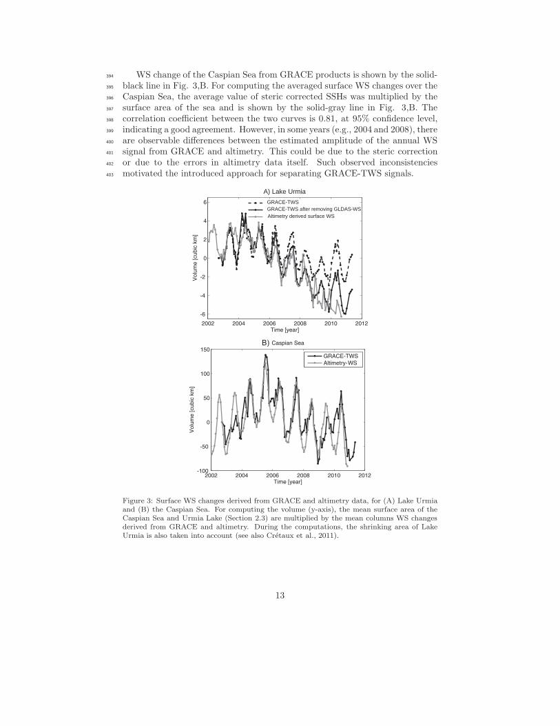
WS change of the Caspian Sea from GRACE products is shown by the solid-394

black line in Fig. 3,B. For computing the averaged surface WS changes over the395

Caspian Sea, the average value of steric corrected SSHs was multiplied by the396

surface area of the sea and is shown by the solid-gray line in Fig. 3,B. The397

correlation coefficient between the two curves is 0.81, at 95% confidence level,398

indicating a good agreement. However, in some years (e.g., 2004 and 2008), there399

are observable differences between the estimated amplitude of the annual WS400

signal from GRACE and altimetry. This could be due to the steric correction401

or due to the errors in altimetry data itself. Such observed inconsistencies402

motivated the introduced approach for separating GRACE-TWS signals.403

A) Lake Urmia

GRACE-TWS after removing GLDAS-WSGRACE-TWS

Altimetry derived surface WS

Figure 3: Surface WS changes derived from GRACE and altimetry data, for (A) Lake Urmiaand (B) the Caspian Sea. For computing the volume (y-axis), the mean surface area of theCaspian Sea and Urmia Lake (Section 2.3) are multiplied by the mean columns WS changesderived from GRACE and altimetry. During the computations, the shrinking area of LakeUrmia is also taken into account (see also Cretaux et al., 2011).

13

5.2. Separation (Adjustment) Results404

The RMS of GRACE-TWS signals in Fig. 2,A clearly demonstrates the405

leakage problem. For instance, a part of the Caspian Sea’s WS leaked into its406

surrounding terrestrial signal or vice versa. In order to separate GRACE-TWS407

changes, we first extracted independent components of WS changes from altime-408

try and GLDAS outputs. The results are shown and described in Figs. A1, A2,409

A3, A4 and A5 of Appendix A. The spatial patterns of the mentioned figures410

were postulated as known patterns in Eq. 4. We also added four other indepen-411

dent components from GLDAS data to Eq. 4. Note that, in order to restrict the412

length of the paper, spatial patterns of IC3 to IC6 are not shown in Appendix413

A. The adjusted temporal patterns of surface and terrestrial WS changes are414

computed using Eq. 4 and are shown in Figs. 4 and 5, respectively. In this415

paper, the temporal components are scaled by their standard deviations to be416

unit-less. Spatial patterns of the figures in Appendix A and B are scaled by the417

standard deviations of their corresponding temporal components to represent418

anomaly maps of WS in millimeter.419

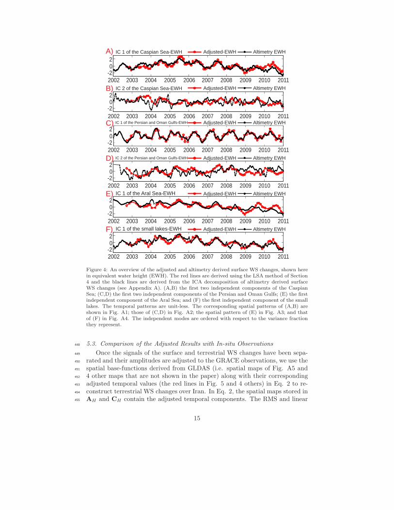
From the annual patterns of surface WS changes, i.e. Fig. 4, A, C, E and420

F, the amplitude of the adjusted signals are comparable to those of altime-421

try derived surface WS (EWH) changes. Comparing the adjusted inter-annual422

changes of surface WS changes (the black lines in Fig. 4,B and D) to their423

altimetry-derived estimates (the red lines in Fig. 4,B and D) shows that the424

adjusted values (i.e. coming from GRACE products) are smoother compared425

to the altimetry results. This is also true for the annual component of the Aral426

Sea (compare the red and black lines in Fig. 4,E). Investigating the reason for427

this difference may be the subject of future research.428

From the adjusted results, we estimate the amplitude of annual surface WS429

changes of the Caspian Sea to be 150 mm, whereas amplitudes of 101 mm and430

71mm are obtained for the Persian and Oman Gulfs, respectively. Fig. 4, E431

indicates a negative linear trend of ∼20 mm/yr during 2002 to 2011 over the432

Aral Sea.433

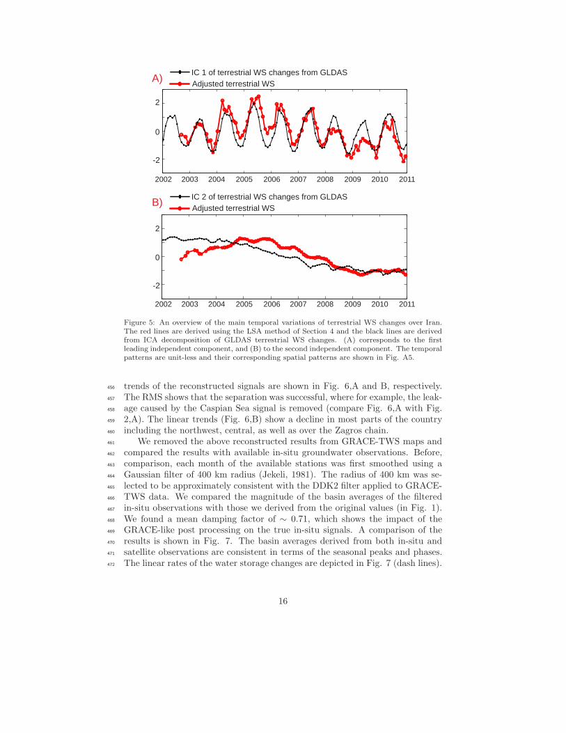
IC1 in Fig. 5,A compares the adjusted value of annual terrestrial WS changes434

with the WS output of GLDAS. Although, the phase of the signal is comparable,435

the amplitudes of the signal differ over the years. For instance, an attenuation436

of the annual amplitudes in the years 2008 and 2009, derived from GRACE437

(the red line in the temporal pattern of IC1) could be related to the prolonged438

drought condition over Iran (Shean, 2008). This impact is not fully reflected in439

the GLDAS outputs (the black line in Fig. 5,A). IC2 of GLDAS (the black line440

in Fig. 5,B) shows an overall decline of terrestrial WS changes mainly over the441

central and north-western parts of Iran (see the spatial map of IC2 in Fig. A5).442

The adjusted value of IC2 (the red line in Fig. 5,B) shows that the drought443

trend actually starts from 2005. The adjusted results are more consistent with444

the drought behaviour we found for the small lakes of the country and also in-445

situ observations, with all showing a decline after 2005. We estimate an average446

decline of 15 mm/yr water column during 2005 to 2011 over central Iran.447

14

IC 1 of the Caspian Sea-EWH Adjusted-EWH Altimetry EWH

IC 2 of the Caspian Sea-EWH

IC 1 of the Persian and Oman Gulfs-EWH

IC 1 of the Aral Sea-EWH

IC 1 of the small lakes-EWH

2002 2003 2004 2005 2006 2007 2008 2009 2010 2011-202

2002 2003 2004 2005 2006 2007 2008 2009 2010 2011-202

2002 2003 2004 2005 2006 2007 2008 2009 2010 2011-202

A)

B)

C)

2002 2003 2004 2005 2006 2007 2008 2009 2010 2011-202

D)

E)

F)

IC 2 of the Persian and Oman Gulfs-EWH

Adjusted-EWH Altimetry EWH

Adjusted-EWH Altimetry EWH

Adjusted-EWH Altimetry EWH

Adjusted-EWH Altimetry EWH

Adjusted-EWH Altimetry EWH

2002 2003 2004 2005 2006 2007 2008 2009 2010 2011-202

2002 2003 2004 2005 2006 2007 2008 2009 2010 2011-202

Figure 4: An overview of the adjusted and altimetry derived surface WS changes, shown herein equivalent water height (EWH). The red lines are derived using the LSA method of Section4 and the black lines are derived from the ICA decomposition of altimetry derived surfaceWS changes (see Appendix A). (A,B) the first two independent components of the CaspianSea; (C,D) the first two independent components of the Persian and Oman Gulfs; (E) the firstindependent component of the Aral Sea; and (F) the first independent component of the smalllakes. The temporal patterns are unit-less. The corresponding spatial patterns of (A,B) areshown in Fig. A1; those of (C,D) in Fig. A2; the spatial pattern of (E) in Fig. A3; and thatof (F) in Fig. A4. The independent modes are ordered with respect to the variance fractionthey represent.

5.3. Comparison of the Adjusted Results with In-situ Observations448

Once the signals of the surface and terrestrial WS changes have been sepa-449

rated and their amplitudes are adjusted to the GRACE observations, we use the450

spatial base-functions derived from GLDAS (i.e. spatial maps of Fig. A5 and451

4 other maps that are not shown in the paper) along with their corresponding452

adjusted temporal values (the red lines in Fig. 5 and 4 others) in Eq. 2 to re-453

construct terrestrial WS changes over Iran. In Eq. 2, the spatial maps stored in454

AH and CH contain the adjusted temporal components. The RMS and linear455

15

IC 1 of terrestrial WS changes from GLDASAdjusted terrestrial WS

2002 2003 2004 2005 2006 2007 2008 2009 2010 2011

-2

0

2

A)

B)

2002 2003 2004 2005 2006 2007 2008 2009 2010 2011

-2

0

2

IC 2 of terrestrial WS changes from GLDASAdjusted terrestrial WS

Figure 5: An overview of the main temporal variations of terrestrial WS changes over Iran.The red lines are derived using the LSA method of Section 4 and the black lines are derivedfrom ICA decomposition of GLDAS terrestrial WS changes. (A) corresponds to the firstleading independent component, and (B) to the second independent component. The temporalpatterns are unit-less and their corresponding spatial patterns are shown in Fig. A5.

trends of the reconstructed signals are shown in Fig. 6,A and B, respectively.456

The RMS shows that the separation was successful, where for example, the leak-457

age caused by the Caspian Sea signal is removed (compare Fig. 6,A with Fig.458

2,A). The linear trends (Fig. 6,B) show a decline in most parts of the country459

including the northwest, central, as well as over the Zagros chain.460

We removed the above reconstructed results from GRACE-TWS maps and461

compared the results with available in-situ groundwater observations. Before,462

comparison, each month of the available stations was first smoothed using a463

Gaussian filter of 400 km radius (Jekeli, 1981). The radius of 400 km was se-464

lected to be approximately consistent with the DDK2 filter applied to GRACE-465

TWS data. We compared the magnitude of the basin averages of the filtered466

in-situ observations with those we derived from the original values (in Fig. 1).467

We found a mean damping factor of ∼ 0.71, which shows the impact of the468

GRACE-like post processing on the true in-situ signals. A comparison of the469

results is shown in Fig. 7. The basin averages derived from both in-situ and470

satellite observations are consistent in terms of the seasonal peaks and phases.471

The linear rates of the water storage changes are depicted in Fig. 7 (dash lines).472

16

50°

50°

60°

60°

30° 30°

40° 40°

-20 -10 0 10 20[mm]

50°

50°

60°

60°

30° 30°

40° 40°

0 50 100[mm]

A) RMS of the terrestrial waterstorage changes after the adjustment,

for the period of October 2002 to May 2011

B) Linear trends of the terrestrial waterstorage changes after the adjustment,

for the period of October 2002 to May 2011

Figure 6: An overview of the reconstructed terrestrial water storage changes over Iran. (A)the RMS of the terrestrial TWS changes after adjusting GRACE-TWS changes (cf. Fig. 2,A)to the base-functions of GLDAS-derived terrestrial WS changes, and (B) the linear trends ofthe signal in (A).

Basins: Khazar Gulfs Urmia Markazi Hamoon Sarakhs(Basin 1) (Basin 2) (Basin 3) (Basin 4) (Basin 5) (Basin 6)

Groundwater rateof 2003-2005 [mm/yr]: 8.6 5.1 8.5 2.5 1.3 3.7Groundwater rateof 2005-2011 [mm/yr]: -6.7 -6.1 -11.2 -9.1 -3.1 -4.2

Table 1: Basin average trends of groundwater variations over the six main basins of Iranderived from GRACE products.

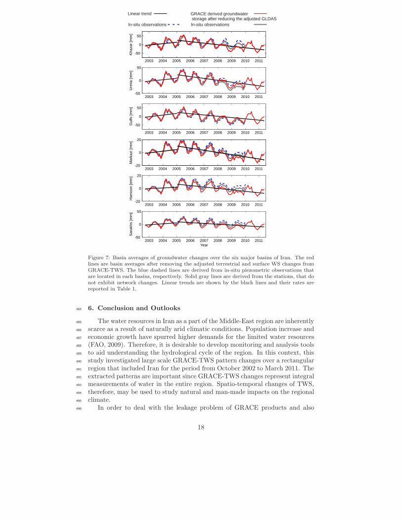
As the figure illustrates, in most of the basins, GRACE derived basin averages473

tend to show steeper slopes compared to the in-situ observations. Part of this474

inconsistency might be the result of network changes in a number of stations.475

We removed those stations from our basin average computations and the new476

results turned out to be more consistent with that of GRACE (solid gray lines).477

The other part of inconsistency might be due to our limited knowledge about478

the porosity parameters used for converting piezometer observations to storage479

values, which can be quite large for some basins (see e.g., Jimenez-Martınez et480

al., 2013). Further research, e.g., involving permanent GPS stations, needs to481

be undertaken to address the problem over the selected region. The results of482

GRACE-derived groundwater rates are summarized in Table 1.483

17

Linear trend GRACE derived groundwaterstorage after reducing the adjusted GLDAS

In-situ observations In-situ observations

2003 2004 2005 2006 2007 2008 2009 2010 2011

-50

0

50

Kha

zar [

mm

]

2003 2004 2005 2006 2007 2008 2009 2010 2011-50

0

50

Urm

ia [m

m]

2003 2004 2005 2006 2007 2008 2009 2010 2011

-50

0

50

Gul

fs [m

m]

2003 2004 2005 2006 2007 2008 2009 2010 2011-20

0

20

Mar

kazi

[mm

]

2003 2004 2005 2006 2007 2008 2009 2010 2011-20

0

20

Ham

oon

[mm

]

2003 2004 2005 2006 2007 2008 2009 2010 2011-50

0

50

Year

Sar

akhs

[mm

]

Figure 7: Basin averages of groundwater changes over the six major basins of Iran. The redlines are basin averages after removing the adjusted terrestrial and surface WS changes fromGRACE-TWS. The blue dashed lines are derived from in-situ piezometric observations thatare located in each basins, respectively. Solid gray lines are derived from the stations, that donot exhibit network changes. Linear trends are shown by the black lines and their rates arereported in Table 1.

6. Conclusion and Outlooks484

The water resources in Iran as a part of the Middle-East region are inherently485

scarce as a result of naturally arid climatic conditions. Population increase and486

economic growth have spurred higher demands for the limited water resources487

(FAO, 2009). Therefore, it is desirable to develop monitoring and analysis tools488

to aid understanding the hydrological cycle of the region. In this context, this489

study investigated large scale GRACE-TWS pattern changes over a rectangular490

region that included Iran for the period from October 2002 to March 2011. The491

extracted patterns are important since GRACE-TWS changes represent integral492

measurements of water in the entire region. Spatio-temporal changes of TWS,493

therefore, may be used to study natural and man-made impacts on the regional494

climate.495

In order to deal with the leakage problem of GRACE products and also496

18

to separate terrestrial from surface WS changes, a least squares adjustment497

approach was applied on the ICA-decomposed terrestrial and surface WS varia-498

tions respectively from GLDAS and altimetry WS outputs. The applied method,499

only relies on the ICA-derived spatial patterns of the hydrological model and500

altimetry observations, which remain invariant in the adjustment. In the ad-501

justment step, the temporal components are estimated from GRACE-TWS data502

(Section 5.2). Adjusted terrestrial WS over Iran showed an overall declining503

trend over the country (Fig. 6,B). In Section 5.3, we demonstrated that the es-504

timated groundwater storages are in a good agreement with in-situ piezometric505

observations. Furthermore, for the first time, this study offers GRACE-derived506

basin averaged groundwater changes for the six main basins of Iran (basins are507

selected according to FAO, 2009). Our estimates of the linear trends of WS508

changes for the period of 2003 to 2005 and the drought period of 2005 to 2011.3509

are shown in Table 1. In view of the low availability of renewable water resources510

in all the basins, in particular, the Markazi and Urmia basins, the results may511

be an important incentive for the water resource management of Iran. Note512

that the area of some of our processed basins, for instance Urmia and Sarakhs,513

are relatively small and might not meet the nominal resolution of the GRACE-514

TWS products. However, the strong WS signal of the basins and the proposed515

optimal processing method allowed retrieval of water storage variations.516

At the root of the presented separation procedure lies the ICA-decomposition517

of the GLDAS and altimetry outputs. Such decompositions contain errors as a518

result of the short length of observations, as well as the errors of observations519

themselves. Including those errors in the least squares procedure may poten-520

tially improve the results but falls outside the scope of the current research. The521

performed separation approach has the potential to be improved by adding extra522

information on the patterns of water storage variations over the Mesopotamia523

region, which covers the Tigris/Euphrates River system, Lake Van etc., (see524

e.g., Voss et al., 2013). The contribution of such base-functions in the inversion525

will, however, be marginal and concentrated over the basins located at the west526

part of the country (i.e. basins 2 and 3). The relationship between WS changes527

in the six major basins of Iran and climate variability such as decadal rainfall528

anomalies and large scale ocean-atmospheric patterns of e.g., the El Nino South-529

ern Oscillation phenomenon might be helpful for understanding the water cycle530

of the region.531

Acknowledgement532

The authors thank the editor M. Bauer and the anonymous reviewer for533

the helpful remarks, which improved the manuscript considerably. E. Forootan534

and J. Kusche are grateful for the financial support provided by the German535

Research Foundation (DFG) under the project BAYES-G. E. Forootan thanks536

L. Moxey (the Operations Manager of NOAA OceanWatch - Central Pacific)537

for the fruitful discussions on altimetry of the Caspian Sea. He also thanks L.538

Longuevergne (Universite de Rennes1) for his useful comments on the performed539

investigations. The authors also thank Y. Hemmati (Iranian Water-resource540

19

Research Center) for providing the in-situ observations. We are grateful for the541

satellite and model data used in this study. This is a TIGeR Publication no.542

491.543

Abbaspour, K.C., Faramarzi, M., Seyed Ghasemi, S., & Yang, H. (2009). Assessing the impact of climate544change on water resources in Iran. Water Resources Research, 45, W10434, doi:10.1029/2008WR007615.545

Ardakani, R. (2009). Overview of Water Management in Iran. Proceeding of Regional Center on Urban Water546Management, Tehran, Iran.547

Avsar, N.B., & Ustun, A. (2012). Analysis of regional time-variable gravity using548GRACE’s 10-day solutions. FIG Working Week 2012, Knowing to manage the territory,549protect the environment, evaluate the cultural heritage, Rome, Italy, 6-10 May 2012,550http://www.fig.net/pub/fig2012/papers/ts04b/TS04B avsar ustun 5724.pdf. (accessed date: May 2013)551

Awange, J.L., Fleming, K.M., Kuhn, M., Featherstone, W.E., Heck, B., & Anjasmara, I. (2011). On the552suitability of the 4◦ × 4◦ GRACE mascon solutions for remote sensing Australian hydrology. Remote Sensing553of Environment, 115, 864-875. doi: 10.1016/j.rse.2010.11.014.554

Awange, J., Forootan, E., Kusche, J., Kiema, J.K.B., Omondi, P., Heck, B., Fleming, K., Ohanya, S., &555Goncalves, R.M. (2013). Understanding the decline of water storage across the Ramser-lake Naivasha using556satellite-based methods. Advances in Water Resources, 60, 7-23, doi:10.1016/j.advwatres.2013.07.002.557

Bari-Abarghouei, H., Asadi-Zarch, M.A., Dastorani, M.T., Kousari, M.R., & Safari-Zarch, M. (2011). The558survey of climatic drought trend in Iran. Stochastic Environmental Research and Risk Assessment, 25 (6),559851-863, doi:10.1007/s00477-011-0491-7.560

Baur, O., Kuhn, M., & Featherstone, W.E. (2013). Continental mass change from GRACE over 2002-2011 and561its impact on sea level. Journal of Geodesy, 87 (2), 117-125, doi:10.1007/s00190-012-0583-2.562

Becker, M., Llovel, W., Cazenave, A., Guntner, A., & Cretaux, J.-F. (2010). Recent hydrological behavior563of the East African great lakes region inferred from GRACE, satellite altimetry and rainfall observations.564Comptes Rendus Geoscience, 342(3), 223-233. http://dx.doi.org/10.1016/j.crte.2009.12.010.565

Birkett, C.M. (1995). The global remote sensing of lakes, wetlands and rivers for hydrological and climate566research, in Geoscience and Remote Sensing Symposium, 1995. IGARSS 95. ’Quantitative Remote Sensing for567Science and Applications’, Vol 3, 1979-1981.568

Cardoso J.F., & Souloumiac, A. (1993). Blind beamforming for non-Gaussian signals. In: IEEE proceedings,569362370. doi:10.1.1.8.5684.570

Chambers, D.P. (2006). Observing seasonal steric sea level variations with GRACE and satellite altimetry. J571Geophys Res, 111, C03010, doi:10.1029/2005JC002914.572

Cheng, M., & Tapley, B.D. (2004). Variations in the Earth’s oblateness during the past 28 years. J Geophys573Res, 109, B09402, doi:10.1029/2004JB003028.574

Cretaux, J-F., Jelinski, W., Calmant, S., Kouraev, A., Vuglinski, V., Berge Nguyen, M., Gennero, M-C., Nino,575F., Abarca Del Rio, F., Cazenave, A., & Maisongrande, P. (2011). SOLS: A lake database to monitor in near576real time water level and storage variations from remote sensing data, Journal of Advanced Space Research,5771497-1507, doi:10.1016/j.asr.2011.01.004.578

Duan, J., Shum, C.K., Guo, J., & Huang, Z. (2012). Uncovered spurious jumps in the GRACE atmospheric579de-aliasing data: potential contamination of GRACE observed mass change. Geophys. J. Int., 191, 83-87,580doi:10.1111/j.1365-246X.2012.05640.x.581

FAO, (2009). FAO Water Report 34.582

Farrell, W. E., & Clark, J. A. (1976). On postglacial sea level. Geophysical Journal of the Royal Astronomical583Society, 46(3), 647-667.584

Famiglietti, J.S., Rodell, M. (2013). Water in the balance. Science 340 (6138), 1300-1301,585doi:10.1126/science.1236460.586

Fenoglio-Marc, L., Kusche, J., & Becker, M. (2006). Mass variation in the Mediterranean Sea from587GRACE and its validation by altimetry, steric and hydrologic fields. Geophysical Research Letters, 33(19),588doi:10.1029/2006GL026851.589

Fenoglio-Marc, L., Rietbroek, R., Grayek, S., Becker, M., Kusche, J., & Stanev, E. (2012). Wa-590ter mass variation in the Mediterranean and Black Sea. Journal of Geodynamics, 59-60, 168-182,591http://dx.doi.org/10.1016/j.jog.2012.04.001.592

Flechtner, F. (2007a). AOD1B product description document for product releases 01 to 04. Technical Report,593Geoforschungszentrum (GFZ), Potsdam.594

Flechtner, F. (2007b). GFZ Level-2 processing standards document for level-2 product release 0004, GRACE595327-743, Rev. 1.0. Technical Report, Geoforschungszentrum, Potsdam.596

Forootan, E., Awange, J., Kusche, J., Heck, B., & Eicker, A. (2012), Independent patterns of water mass597anomalies over Australia from satellite data and models. Remote Sensing of Environment, 124, 427-443,598doi:0.1016/j.rse.2012.05.023.599

20

Forootan, E., & Kusche, J. (2013). Separation of deterministic signals, using independent component analysis600(ICA). Stud. Geophys. Geod, Vol.57 (1), 17-26, doi: 10.1007/s11200-012-0718-1.601

Forootan, E., & Kusche, J. (2012). Separation of global time-variable gravity signals into maximally indepen-602dent components. Journal of Geodesy, 86 (7), 477-497, doi:10.1007/s00190-011-0532-5.603

Forootan, E., Didova, O., Kusche, J., & Locher, A. (2013). Comparisons of atmospheric data and reduction604methods for the analysis of satellite gravimetry observations. JGR-Solid Earth, doi: 10.1002/jgrb.50160.605

Frappart, F., Ramillien, G., Leblanc, M., Tweed, S.O., Bonnet, M.P., & Maisongrande, P. (2010). An indepen-606dent component analysis filtering approach for estimating continental hydrology in the GRACE gravity data.607Remote Sens Environ, 115(1), 187-204. doi:10.1016/j.rse.2010.08.017608

Ghandhari, A., & Alavi-Moghaddam, S.M.R. (2011). Water balance principles: A review of studies on five609watersheds in Iran. Journal of Environmental Science and Technology, 4 (5), 465-479, ISSN: 1994-7887,610doi:10.3923/jest.2011.465.479.611

Grippa, M., Kergoat, L., Frappart, F., Araud, Q., Boone, A., de Rosnay, P., Lemoine, J.-M., Gascoin, S.,612Balsamo, G., Ottle, C., Decharme, B., Saux-Picart, S., & Ramillien, G. (2011), Land water storage variability613over West Africa estimated by Gravity Recovery and Climate Experiment (GRACE) and land surface models.614Water Resour. Res., 47, W05549, doi:10.1029/2009WR008856.615

Guntner, A., Stuck, J., Werth, S., Doll, P., Verzano, K., & Merz, B. (2007). A global analysis of temporal and616spatial variations in continental water storage. Water Resour. Res., 43, W05416, doi:10.1029/2006WR005247.617

Guntner, A. (2008). Improvement of global hydrological models using GRACE data, Surv. Geophys., 29, 375-618397.619

Ishii, M., & Kimoto. M. (2009). Reevaluation of historical ocean heat content variations with time-varying620XBT and MBT depth bias corrections. Journal of Oceanography 65, 287-299.621

Jekeli, C. (1981). Alternative methods to smooth the Earth’s gravity field. Technical report rep 327. Depart-622ment of Geodesy and Science and Surveying, Ohio State University, Columbus.623

Jensen, L., Rietbroek, R., & Kusche, J. (2013). Land water contribution to sea level from GRACE and Jason-1624measurements. Journal of Geophysical Research-Oceans, 118 (1), 212226, doi:10.1002/jgrc.20058.625

Jimenez-Martınez, J., Longuevergne, L., Le Borgne, T., Davy, P., Russian, A., & Bour, O. (2013). Temporal626and spatial scaling of hydraulic response to recharge in fractured aquifers: Insights from a frequency domain627analysis. WATER RESOURCES RESEARCH, 49, 1-17, doi:10.1002/wrcr.20260.628

Kampf, J., & Sadrinasab, M. (2006). The circulation of the Persian Gulf: a numerical study. Ocean Sci., 2,62927-41. http://www.ocean-sci.net/2/27/2006/os-2-27-2006.html.630

Klees, R., Revtova, E.A., Gunter, B.C., Ditmar, P., Oudman, E., Winsemius, H.C. & Savenije, H.H.G. (2008).631The design of an optimal filter for monthly GRACE gravity models. Geophysical Journal International, 175(2),632417-432, doi:10.1111/j.1365-246X.2008.03922.x.633

Klees, R., Zapreeva, E.A., Winsemius, H.C., & Savenije, H.H.G. (2007). The bias in GRACE estimates of634continental water storage variations. Hydrology and Earth System Sciences Discussions, 11, 1227-1241.635

Koch, K.R. (1988). Parameter estimation and hypothesis testing in linear models. Springer, New York.636ISBN:978354065257.637

Kosarev, A.N., & Yablonskaya, E.A., (1994). The Caspian Sea. The Netherlands:SPB Academic Publishing,638pp. 260, ISBN-10:9051030886.639

Kouraev, A.V., Cretaux, J.-F., Lebedev, S.A., Kostianoy, A.G., Ginzburg, A.I., Sheremet, N.A., Mamedov,640R., Zakharova, E.A., Roblou, L., Lyard, F., Calmant, S., & Berge-Nguyen, M. (2011). Satellite altimetry641applications in the Caspian Sea (Chapter 13). In Coastal Altimetry, (Eds) S., Kostianoy, A., Cipollini, P., and642Benveniste, J. Springer, 331-366, ISBN:978-3-642-12795-3.643

Kusche, J. (2007). Approximate decorrelation and non-isotropic smoothing of time-variable GRACE-type grav-644ity field models. Journal of Geodesy, 81, 733-749, doi:10.1007/s00190-007-0143-3.645

Kusche, J., Klemann, V., & Bosch, W. (2012). Mass distribution and mass transport in the Earth system.646Journal of Geodynamics, 59-60, 1-8, http://dx.doi.org/10.1016/j.jog.2012.03.003.647

Kusche, J., Schmidt, R., Petrovic, S., & Rietbroek, R. (2009). Decorrelated GRACE time-variable grav-648ity solutions by GFZ, and their validation using a hydrological model. Journal of Geodesy, 83, 903-913,649doi:10.1007/s00190-009-0308-3.650

Lambeck, K., Esat, T.M., & Potter, E.K. (2002). Links between climate and sea levels for the past three million651years. Nature., 2002 Sep 12, 419(6903), 199-206.652

Llovel, W., Becker, M., Cazenave, A., Cretaux, J-F., & Ramillien, G. (2010). Global land water storage653change from GRACE over 2002-2009; Inference on sea level. Comptes Rendus Geoscience, 342, (3), 179-188,654doi:http://dx.doi.org/10.1016/j.crte.2009.12.004.655

Longuevergne, L., Scanlon, B.R., & Wilson, C.R. (2010). GRACE Hydrological estimates for small basins: Eval-656uating processing approaches on the High Plains Aquifer, USA. Water Resources Research, 46 (11), W11517,657doi:10.1029/2009WR008564.658

21

Longuevergne, L., Wilson, C.R., Scanlon, B.R., & Cretaux, J-F. (2012). GRACE water storage estimates for659the Middle East and other regions with significant reservoir and lake storage. Hydrol. Earth Syst. Sci. Discuss.,6609, 11131-11159, doi:10.5194/hessd-9-11131-2012.661

Modarres, R. (2006). Regional precipitation climates of Iran. Journal of Hydrology (NZ) 45 (1), 13-27,662ISSN:0022-1708.663

Mohammadi-Ghaleni, M., & Ebrahimi, K. (2011). Assessing impact of irrigation and drainage network on664surface and groundwater resources - case study: Saveh Plain, Iran. ICID 21’st International Congress on665Irrigation and Drainage, 15-23 October 2011, Tehran, Iran.666

Motagh, M., Walter, T. R., Sharifi, M. A., Fielding, E., Schenk, A., Anderssohn, J., & Zschau, J. (2008). Land667subsidence in Iran caused by widespread water reservoir overexploitation. Geophysical Research Letters, 35,668L16403, doi:10.1029/2008GL033814.669

Noory H., van der Zee, S.E.A.T.M., Liaghat, A.-M., Parsinejad, M., & van Dam, J.C. (2011). Dis-670tributed agro-hydrological modeling with SWAP to improve water and salt management of the Voshm-671gir irrigation and drainage network in Northern Iran. Agricultural Water Management, 98, 1062-1070,672doi:10.1016/j.agwat.2011.01.013.673

Pous, S.P., Carton, X., & Lazure, P. (2004). Hydrology and circulation in the Strait of Hormuz and the Gulf674of Oman, Results from the GOGP99 Experiment: 2. Gulf of Oman. Journal of Geophysical Research, 109,675C12038, doi:10.1029/2003JC002146.676

Preisendorfer, R. (1988). Principal component analysis in Meteorology and Oceanography. Elsevier: Amster-677dam, 426 pages. ISBN:0444430148.678

Ramillien, G., Famiglietti, J.S., & Wahr, J. (2008). Detection of continental hydrology and glaciology signals679from GRACE: a review, Surv. Geophys., 29, 361-374, doi:10.1007/s10712-008-9048-9.680

Reynolds, R.W., Rayne, N.A., Smith, T.M., Stokes, D.C., & Wang, W. (2002). An improved in situ and satellite681SST analysis for climate. J. Clim., 15 (2002), pp. 1609-1625.682

Rietbroek, R., Brunnabend, S.E., Dahle, C., Kusche, J., Flechtner, F., Schroter, J., & Timmermann, R. (2009).683Changes in total ocean mass derived from GRACE, GPS, and ocean modeling with weekly resolution. J Geophys684Res., 114, C11004, doi:10.1029/2009JC005449.685

Rietbroek, R., Brunnabend, S.E., Kusche, J., & Schroter, J. (2012). Resolving sea level contributions686by identifying fingerprints in time-variable gravity and altimetry. Journal of Geodynamics, 59, 72-81,687http://dx.doi.org/10.1016/j.jog.2011.06.007.688

Rodell, M., Chen. J., Kato, H., Famigietti, J., Nigro, J., & Wilson, C. (2007). Estimating ground water storage689changes in the Mississippi River basin (USA) using GRACE. Hydrogeol. J. 15 159-166. doi:10.1007/s10040-006-6900103-7.691

Rodell, M., & Famiglietti, J.S. (2001), An analysis of terrestrial water storage variations in Illinois with692implications for the Gravity Recovery and Climate Experiment (GRACE), Water Resour. Res., 37(5), 1327-6931340, doi:10.1029/2000WR900306.694

Rodell, M., Houser, P.R., Jambor, U., Gottschalck, J., Mitchell, K., Meng, K., Arsenault, C.-J., Cosgrove, B.,695Radakovich, J., Bosilovich, M., Entin, J.K., Walker, J.P., Lohmann, D., & Toll, D. (2004). The Global Land696Data Assimilation System. Bulletin of the American Meteorological Society, 85 (3), 381-394.697

Rodell, M., Velicogna, I., & Famiglietti, J.S. (2009). Satellite-based estimates of groundwater depletion in698India. Nature, 460, 999-1002, doi:10.1038/nature08238.699

Sarraf, M., Owaygen, M., Ruta, G., & Croitoru, L. (2005). Islamic Republic of Iran: Cost assessment of700environmental degradation, Tech. Rep. 32043-IR, World Bank, Washington, D. C.701

Schmeer, M., Schmidt, M., Bosch, W., & Seitz, F. (2012). Separation of mass signals within GRACE monthly702gravity field models by means of empirical orthogonal functions. Journal of Geodynamics, 59-60, 124-132,703doi:10.1016/j.jog.2012.03.001.704

Schmidt, M., Seitz, F., & Shum, C.K. (2008). Regional fourdimensional hydrological mass variations705from GRACE, atmospheric flux convergence, and river gauge data, J. Geophys. Res., 113, B10402,706doi:10.1029/2008JB005575.707

Schnitzer, S., Seitz, F., Eicker, A., Guntner, A., Wattenbach, M., & Menzel, A. (2013). Estimation of soil loss708by water erosion in the Chinese Loess Plateau using universal soil loss equation and GRACE. Geophys. J. Int.,709doi:10.1093/gji/ggt023.710

Sharifi, M.A., Forootan, E., Nikkhoo, M., Awange, J., & Najafi-Alamdari, M. (2013). A point-wise least711squares spectral analysis (LSSA) of the Caspian Sea level fluctuations, using TOPEX/Poseidon and Jason-1712observations. Advances in Space Research, 51 (5), 858-873, http://dx.doi.org/10.1016/j.asr.2012.10.001.713

Shean, M. (2008). IRAN: 2008/09 wheat production declines due to drought.714Commodity intelligence report. United States Department of Agriculture (USDA),715http://www.pecad.fas.usda.gov/highlights/2008/05/Iran may2008.html. Access date: 20.02.2013.716

Shum, C.K., Jun-Yi, G., Hossain, F., Duan, J., Alsdorf, D.E., Duan, X-J, Kuo, C-Y., Lee, K., Schmift, M.,717& Wang, L. (2011). Inter-annual Water Storage Changes in Asia from GRACE Data. In R. Lal et al. (eds.),718Climate Change and Food Security in South Asia, doi:10.1007/978-90-481-9516-9 6.719

22

Swenson, S., & Wahr, J. (2002). Methods for inferring regional surface-mass anomalies from Gravity Recovery720and Climate Experiment (GRACE) measurements of time-variable gravity. Journal of Geophysical Research,721107 (B9), ETG 3-1 - 3-13, doi:10.1029/2001JB000576.722

Swenson, S., & Wahr, J. (2006). Post-processing removal of correlated errors in GRACE data. Geophys Res723Lett., 33, L08402, doi:10.1029/2005GL025285.724

Swenson, S., & Wahr, J. (2007). Multi-sensor analysis of water storage variations of the Caspian Sea. Geophys725Res Lett., 34, L16401, doi:10.1029/2007GL030733.726

Syed, T.H., Famigletti, J.S., Chen, J., Rodell, M., Seneviratne, S.I., Viterbo, P., & Wilson, C.R. (2005).727Total basin discharge for the Amazon and Mississippi River basins from GRACE and a land-atmosphere water728balance, Geophys. Res. Lett., 32, L24404, doi:10.1029/2005GL024851.729

Syed, T.H., Famiglietti, J.S., Rodell, M., Chen, J., & Wilson, C.R. (2008). Analysis of terrestrial water storage730changes from GRACE and GLDAS, Water Resources Research, 44, W02433, doi:10.1029/2006WR005779.731

Tapley, B., Bettadpur, S., Ries, J., Thompson, P., & Watkins, M. (2004a). GRACE measurements of mass732variability in the Earth system. Science, 305, 503-505. http://dx.doi.org/10.1126/science.1099192.733

Tapley, B., Bettadpur, S., Watkins, M., & Reigber, C. (2004b). The gravity recovery and cli-734mate experiment: Mission overview and early results. Geophysical Research Letters, 31, L09607.735http://dx.doi.org/10.1029/2004GL019920.736

Van Camp, M., Radfar, M., Martens, K., & Walraevens, K. (2012). Analysis of the groundwater resource737decline in an intramountain aquifer system in Central Iran. GEOLOGICA BELGICA (2012) 15/3: 176-180.738

van Dijk, A.I.J.M. (2011) Model-data fusion: using observations to understand and reduce uncertainty in hy-739drological models. 19th International Congress on Modelling and Simulation, Perth, Australia, 12-16 December7402011. http://mssanz.org.au/modsim2011/index.html741

van Dijk, A.I.J.M., Renzullo, L.J., & Rodell, M. (2011). Use of Gravity Recovery and Climate Experiment742terrestrial water storage retrievals to evaluate model estimates by the Australian water resources assessment743system. Water Resour. Res., 47, W11524, doi:10.1029/2011WR010714.744

Voss, K.A., Famiglietti, J.S., Lo, M-H., de Linage, C., Rodell, M., & Swenson, S.C. (2013). Groundwater745depletion in the Middle East from GRACE with implications for transboundary water management in the746Tigris-Euphrates-Western Iran region, Water Resour. Res., 49, doi:10.1002/wrcr.20078.747

Wahr, J., Molenaar, M., & Bryan, F. (1998). Time variability of the Earth’s gravity field: Hydrological and748oceanic effects and their possible detection using GRACE. Journal of Geophysical Research 103 (B12), 30205-74930229, doi:10.1029/98JB02844.750

Wahr, J., Swenson, S., Velicogna, I., & Zlotnicki, V. (2004). Time-variable gravity from GRACE: First results,751Geophysical Research Letters paper 10.1029/2004GL019779.752

Werth, S., Guntner, A., Schmidt, R., & Kusche, J. (2009). Evaluation of GRACE filter tools from a hy-753drological perspective. Geophysical Journal International, 179, 1499-1515, http://dx.doi.org/10.1111/j.1365-754246X.2009.04355.x.755

23

Appendix A756

Extracting Independent Components from GLDAS and Altimetry WS Changes757

ICA is applied on the data sets on each GLDAS and altimetry data sets758

using Eqs. 2 and 3 (see the details of application in e.g., Forootan and Kusche,759

2012). For altimetry products, ICA was individually implemented on (i) the760

Caspian Sea, (ii) the Persian and Oman Gulfs, (iii) the Aral Sea, and finally761

(iv) the other small lakes. The results are depicted in Figs. A1, A2, A3 and A4.762

Note that, similar to the main text, all the temporally independent components763

(ICs) are unit-less and the spatial patterns are given in millimeters.764

Fig. A1 shows the first two independent modes, accounting for 93% of the765

surface WS variance in the Caspian Sea. The remaining 7% of the variance766

are noisy and are not shown here. IC1 shows an annual behaviour along with767

two linear trends, one from January 2002 to December 2005 with a rate of 108768

mm/yr and the other from January 2006 to October 2008 with a rate of -152769

mm/yr. IC2 indicates the main inter-annual variability from which, the spatial770

pattern of IC2 shows that the northern part of Caspian exhibits stronger inter-771

annual variations compared to the central and southern parts (see Fig. A1).772

This can be related to the climatic extremes, which are more pronounced in the773

northern part of the Caspian sea inducing stronger mass variations (Kouraev et774

al., 2011; Sharifi et al., 2013).775

The ICA decomposition of WS changes of the Persian and Oman Gulfs also776

shows two significant components explaining 89% of the total variance. IC1777

shows an annual behaviour with a dipole spatial structure over the two gulfs778

(see Fig. A2, spatial pattern of IC1). IC2 shows a superposition of inter-annual779

variability and a positive linear trend (9 mm/yr) dominant mainly over the780

head of the Persian Gulf, where Lambeck et al. (2002) reported a rise due to781

the post glacial rebound.782

Fig. A3 shows that only one of the independent component of surface WS783

changes (corresponding to 89% of the total variance) over the Aral Sea is sta-784

tistically significant. IC1 of Aral shows the shrinking of the sea with an average785

linear rate of 300 mm/yr. Results of ICA, applied on surface WS changes of786

the small lakes and reservoirs, are shown in Fig. A4. While only the first IC787

corresponding to 93% of total variance was significant, it shows that most of788

the surface water of Iran, specifically after the year 2005, are losing water. This789

situation might be related to the long-term drought condition of the country,790

see e.g. Bari-Abarghouei et al. (2011).791

For brevity we only present the first two independent components of GLDAS792

data, explaining 71% of the total variance of terrestrial WS changes in Fig. A5.793

The temporal pattern of IC1 shows the dominant annual variation, while the794

spatial pattern of IC1 is mainly concentrated over north and west Iran. The795

temporal pattern of IC2 shows an overall linear trend (during 2002 to 2010)796

corresponding to a decrease of WS over the Markazi and Urmia Basins (see797

Fig. A5, spatial pattern of IC2). The derived trend appears to differ from the798

observations of WS changes, e.g., over Urmia (Fig. 3,A) and other small lakes799

(Fig. A4), where the WS decrease starts from 2005.800

24

We should mention here, that to reconstruct 90% of the GLDAS data, one801

needs to select at least the first six independent components of GLDAS. The802

temporal behaviours of the remaining four independent components of GLDAS803

were difficult to interpret and are therefore not plotted. These components were,804

however, still used in the adjustment procedure.805

Appendix B806

Self-gravitational Impact807

The strong seasonal mass fluctuations in the Caspian Sea will cause a time808

variable change in the geoid. On very short time scales (typically days), the809

ocean will adapt itself to this new equipotential surface, similar to the tidal810

response of the ocean. This implies that the sea level in the Gulfs and the811

Black Sea are (indirectly) influenced by the variations in the Caspian Sea. This812

effect is known as the self-consistent sea level response and has already been813

described in Farrel and Clarke (1976). When unaccounted for, this effect may814

potentially mix signal between the base-functions discussed in the main text.815

We, therefore, quantified its magnitude by taking the steric corrected sea level816

from altimetry and computed the self consistent sea level response according817

to Rietbroek et al. (2012). Fig. B1 shows the RMS of this effect. The effect818

is strongest in the Black Sea, since it is located closest to the Caspian Sea.819

However the magnitude of the effect is very small compared to the hydrological820

and oceanic signal sought such that it is not expected to influence the results.821

822

25

Spatial pattern of IC 1 Spatial pattern of IC 2

10.8 cm/year -15.2 cm/yearRate (Jan.2002 to Dec-2005): Rate (Jan.2006 to Jan-2011):

2003 2005 2007 2009 2011-3

-2

-1

0

1

2

32003 2005 2007 2009 2011

-3

-2

-1

0

1

2

3

Figure A1: Results of the ICA method applied to the steric corrected SSHdata (surface WS changes) over the Caspian Sea. The results are ordered

according to their signal strength.

Spatial pattern of IC 1

Spatial pattern of IC 2

Rate(Jan.2002 to Jan.2011):0.9 cm/year

2003 2005 2007 2009 2011-3-2-10

123

2003 2005 2007 2009 2011-3-2-10

123

Figure A2: Results of the ICA method applied to the steric corrected SSHdata (surface WS changes) over the Persian and Oman Gulfs. The results are

ordered according to their signal strength.

26

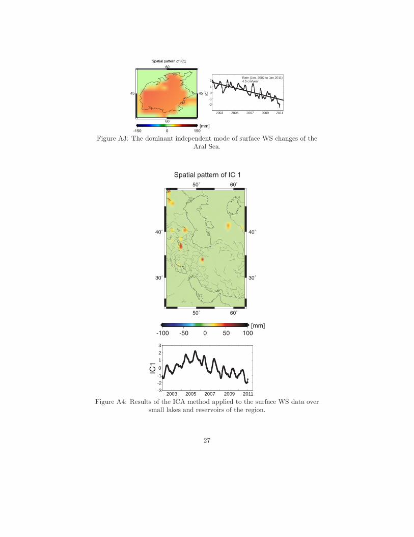
2003 2005 2007 2009

-2

-1

0

1

2

Spatial pattern of IC1

60

60

45 45

2011

Rate (Jan. 2002 to Jan.2011)4.5 cm/year

Figure A3: The dominant independent mode of surface WS changes of theAral Sea.

2003 2005 2007 2009 2011-3-2-10123

Figure A4: Results of the ICA method applied to the surface WS data oversmall lakes and reservoirs of the region.

27

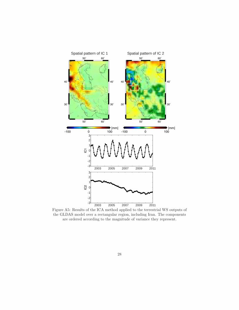
Spatial pattern of IC 1 Spatial pattern of IC 2

2003 2005 2007 2009 2011

2003 2005 2007 2009 2011

-3-2

-1

0

123

-3-2

-1

0

123

Figure A5: Results of the ICA method applied to the terrestrial WS outputs ofthe GLDAS model over a rectangular region, including Iran. The components

are ordered according to the magnitude of variance they represent.

28

Figure B1: RMS of the self gravitational effect of the Caspian Sea’s levelvariations (steric corrected altimetry) on relative sea level in the Gulfs and the

Black Sea.

29