Embed Size (px)
Citation preview

Prepared by Sentinel-2 PDGS Project Team Reference GMES-GSEG-EOPG-PL-10-0054 Issue 1 Revision 6 Date of Issue 22 December 2014 Status Authorised Document Type PL
ESA UNCLASSIFIED – For Official Use
ESA UNCLASSIFIED – For Official Use
esrin
Via Galileo Galilei
Casella Postale 64 00044 Frascati
Italy T +39 06 941801
F +39 06 94180280 www.esa.int
Sentinel-2 Calibration and Validation Plan for the Operational Phase

Page 2/120 Date 22 December 2014 Issue 1 Rev 6
ESA UNCLASSIFIED – For Official Use
ESA UNCLASSIFIED – For Official Use
Title Sentinel-2 Calibration and Validation Plan for the Operational Phase Issue 1 Revision 6 Author Sentinel-2 PDGS Project Team Date 22 December 2014 Approved by Signature and Date
F. Gascon (EOP-GMQ)
O. Colin (EOP-GSG)
B. Hoersch (EOP-GS)
Reason for change Issue Revision Date Draft 1 0-draft 30 June 2011 First issue 1 0 01 March 2012 Update for PDGS MPA ITT 1 1 15 May 2012 Update for MPA KO 1 2 01 August 2012 Update for editorial changes 1 3 20 September 2012 Update for MPC KO 1 4 20 February 2013 Update for MPC SDR 1 5 25 July 2014 Update for MPC and MPA 1 6 22 December 2014
Issue 1 Revision 0 Reason for change Paragraph(s) Updates from S2 PDGS PDR RIDs: 443, 435, 374, 272, 371, 369. 1.9, 2, 3 Updates considering RIDs from TAS. 2, 3, 5

Page 3/120 Date 22 December 2014 Issue 1 Rev 6
ESA UNCLASSIFIED – For Official Use
ESA UNCLASSIFIED – For Official Use
Issue 1 Revision 1 Reason for change Paragraph(s) Major updates on the Nominal Radiometric Activities. 3.2.2.5 Clarifications on the SNR Validation 3.3.2.7 General updates - Issue 1 Revision 2 Reason for change Paragraph(s) Updated sections (including clarification of methods description). 3.2, 3.3, 4.2, 4.3, 5.2, 5.3, 6.1, 6.2, 6.3,
6.4, 6.5, 6.6, 6.7 Updates from S2 PDGS PDR RIDs: 473, 471, 372, 371 and 370. -
Issue 1 Revision 3 Reason for change Paragraph(s) Section 6.1 (from Issue 1 Revision 2) moved to end of Section 6 6.7 Minor editorials -
Issue 1 Revision 4 Reason for change Paragraph(s) Reference documents added. 1.5 Included details on diffuser BRDF interpolation 6.5 Mission Manager added in the approval list Page 2 Updated section 6.7 cf. Jira Issue MPA-797 6.7 Editorials all
Issue 1 Revision 5 Reason for change Paragraph(s) Document title updated Cover page Updates on reference/applicable documents and acronyms lists 1.4, 1.5 and 1.6 Update of the MSI Radiometric Model 3.2.2.2 Update of the Level-1 Processing Radiometric Model 3.2.2.3 Update of Relative Gains and Absolute Radiometric Calibration outputs 3.2.2.5.3.4 and 3.2.2.5.3.4 Removal of alpha/beta noise parameters conversion from radiance to reflectance units
3.3.2.7.4
Update in method description 6.4.5 Editorials -

Page 4/120 Date 22 December 2014 Issue 1 Rev 6
ESA UNCLASSIFIED – For Official Use
ESA UNCLASSIFIED – For Official Use
Issue 1 Revision 6 Reason for change Paragraph(s) Paragraph deleted. 3.1 Clarification on use of nominal mode. 3.2.2.1 Updated baseline for SWIR on-ground equalisation model. Page 33 Dark signal calibration inputs updated. Page 37 Method description updated. Page 41 Astrium SAS replaced by Airbus D&S Page 49 Update of on-board and on-ground model for SWIR bands Pages 29, 30, 31, page 38, page 40, Reference to MSI manual added (FOM-MSI) Page 10, 18

Page 5/120 Date 22 December 2014 Issue 1 Rev 6
ESA UNCLASSIFIED – For Official Use
ESA UNCLASSIFIED – For Official Use
Table of contents
1 Introduction ......................................................................................................................................... 8 1.1 Purpose of the Document .......................................................................................................................... 8 1.2 Background .................................................................................................................................................... 8 1.3 Document Overview ................................................................................................................................... 8 1.4 Applicable Documents ............................................................................................................................... 9 1.5 Reference Documents ................................................................................................................................ 9 1.6 Acronyms ..................................................................................................................................................... 10 1.7 Definition, Terms and Conventions .................................................................................................... 12 1.7.1 Calibration ................................................................................................................................................................. 12 1.7.2 Validation ................................................................................................................................................................... 12 1.7.3 Accuracy ..................................................................................................................................................................... 12 1.7.4 Precision ..................................................................................................................................................................... 12 1.7.5 Uncertainty ................................................................................................................................................................ 13 1.7.6 Other Definitions .................................................................................................................................................... 13
1.8 MSI Instrument Overview ...................................................................................................................... 14 1.9 Products Quality Requirements .......................................................................................................... 20 1.9.1 Level-‐1 Radiometric Quality Requirements ............................................................................................... 20 1.9.2 Level-‐1 Geometric Quality Requirements .................................................................................................... 22 1.9.3 Level-‐2A Quality Requirements ....................................................................................................................... 23
1.10 Mission Performance Centre .............................................................................................................. 23 2 Overview of the Calibration and Validation Activities ......................................................... 23
3 Level-‐1 .................................................................................................................................................. 27 3.1 Introduction ............................................................................................................................................... 27 3.2 Level-‐1 Calibration ................................................................................................................................... 27 3.2.1 Introduction .............................................................................................................................................................. 27 3.2.2 Radiometric Calibration ...................................................................................................................................... 27 3.2.3 Geometric Calibration .......................................................................................................................................... 47
3.3 Level-‐1 Validation ..................................................................................................................................... 59 3.3.1 Introduction .............................................................................................................................................................. 59 3.3.2 Radiometric Validation ........................................................................................................................................ 59 3.3.3 Geometric Validation ............................................................................................................................................ 79
4 Level-‐2A ............................................................................................................................................... 89 4.1 Introduction ............................................................................................................................................... 89 4.2 Level-‐2A Calibration ................................................................................................................................ 89 4.3 Level-‐2A Validation .................................................................................................................................. 89
5 Annex A: Calibration and Validation Test Sites ...................................................................... 90 5.1 Introduction ............................................................................................................................................... 90 5.2 CEOS Test Sites ........................................................................................................................................... 90 5.2.1 Frenchman Flat (USA) .......................................................................................................................................... 90 5.2.2 La Crau (France) ..................................................................................................................................................... 91

Page 6/120 Date 22 December 2014 Issue 1 Rev 6
ESA UNCLASSIFIED – For Official Use
ESA UNCLASSIFIED – For Official Use
5.2.3 Dome-‐C (Antarctica) ............................................................................................................................................. 92 5.3 Other Test Sites ......................................................................................................................................... 92 5.3.1 Barrax (Spain) .......................................................................................................................................................... 92 5.3.2 Maricopa Fields (USA) .......................................................................................................................................... 93 5.3.3 Ross Ice Shelf (Antarctica) .................................................................................................................................. 93 5.3.4 Lake Ponchartrain Causeway (USA) .............................................................................................................. 93 5.3.5 Bronx Whitestone Bridge (USA) ...................................................................................................................... 94 5.3.6 Manosque (France) ................................................................................................................................................ 94 5.3.7 Bern/Thun (Switzerland) ................................................................................................................................... 94 5.3.8 Cape Town (South Africa) ................................................................................................................................... 95
6 Annex B: Calibration and Validation Complementary Methods Description ............... 96 6.1 Method for the Update of Pixel Status ............................................................................................... 96 6.1.1 Background ............................................................................................................................................................... 96 6.1.2 Objective ..................................................................................................................................................................... 96 6.1.3 Inputs ........................................................................................................................................................................... 96 6.1.4 Outputs ........................................................................................................................................................................ 96 6.1.5 Method Description ............................................................................................................................................... 96
6.2 Method for SWIR Detectors Re-‐arrangement Parameters Generation .................................. 98 6.2.1 Background ............................................................................................................................................................... 98 6.2.2 Objective ..................................................................................................................................................................... 99 6.2.3 Inputs ........................................................................................................................................................................... 99 6.2.4 Outputs ........................................................................................................................................................................ 99 6.2.5 Method Description ............................................................................................................................................... 99
6.3 Method for Dark Signal and Pixel Contextual Offset Correction ............................................ 102 6.3.1 Background ............................................................................................................................................................ 102 6.3.2 Objective .................................................................................................................................................................. 102 6.3.3 Inputs ........................................................................................................................................................................ 102 6.3.4 Outputs ..................................................................................................................................................................... 102 6.3.5 Method Description ............................................................................................................................................ 102
6.4 Method for Diffuser Geometry Modelling ....................................................................................... 103 6.4.1 Background ............................................................................................................................................................ 103 6.4.2 Objective .................................................................................................................................................................. 103 6.4.3 Inputs ........................................................................................................................................................................ 103 6.4.4 Outputs ..................................................................................................................................................................... 104 6.4.5 Method Description ............................................................................................................................................ 104
6.5 Method for Diffuser BRDF Interpolation ........................................................................................ 107 6.5.1 Background ............................................................................................................................................................ 107 6.5.2 Objective .................................................................................................................................................................. 107 6.5.3 Inputs ........................................................................................................................................................................ 107 6.5.4 Outputs ..................................................................................................................................................................... 107 6.5.5 Method ..................................................................................................................................................................... 108
6.6 Method for Data Extraction for Vicarious Validation ................................................................. 108 6.6.1 Background ............................................................................................................................................................ 108 6.6.2 Objective .................................................................................................................................................................. 108 6.6.3 Inputs ........................................................................................................................................................................ 108

Page 7/120 Date 22 December 2014 Issue 1 Rev 6
ESA UNCLASSIFIED – For Official Use
ESA UNCLASSIFIED – For Official Use
6.6.4 Outputs ..................................................................................................................................................................... 109 6.6.5 Method ..................................................................................................................................................................... 110
6.7 Method for Assessing the Noise Model ............................................................................................ 112 6.7.1 Background ............................................................................................................................................................ 112 6.7.2 Objective .................................................................................................................................................................. 114 6.7.3 Inputs ........................................................................................................................................................................ 114 6.7.4 Outputs ..................................................................................................................................................................... 114 6.7.5 Method Description ............................................................................................................................................ 115
7 Annex C: Campaigns ...................................................................................................................... 120 7.1 Introduction ............................................................................................................................................. 120 7.2 CEFLES2 ...................................................................................................................................................... 120

Page 8/120 Sentinel-2 Calibration and Validation Plan for the Operational Phase Date 22 December 2014 Issue 1 Rev 6
ESA UNCLASSIFIED – For Official Use
Appendix A ESA UNCLASSIFIED – For Official Use
1 INTRODUCTION
1.1 Purpose of the Document This document defines the plan, methods and principles of the Calibration and Validation Plan for Sentinel-2 during the operational phase (Phase E2).
1.2 Background Data quality is the aptitude of a product to answer user needs. User needs are not homogeneous and are dependant of each application field (e.g. cartography, forest monitoring, photo-interpretation). Therefore, as an example, the ability to detect and quantify changes in the Earth’s environment depends on sensors that can provide calibrated (known accuracy and precision) and consistent measurements of the Earth’s surface features through time. Calibration and Validation (often referred as Cal/Val) corresponds to the process of updating and validating on-board and on-ground configuration parameters and algorithms to ensure that the product data quality requirements are met. To meet the baseline product quality requirements, a well-defined Calibration and Validation (Cal/Val) plan will be systematically applied. In complement, the operational monitoring of the resulting product-quality will be ensured through well-defined Quality Control procedures. Cal/Val activities will be carried in coordination and cooperation with other CEOS (Committee on Earth Observation Satellites) partners and in line with its quality assurance strategy endorsed by CEOS, the Quality Assurance framework for Earth Observation (QA4EO). Further information on CEOS and QA4EO can be found respectively at http://www.ceos.org/ and http://qa4eo.org/. The calibration and the validation activities presented in this document are under the responsibility of Sentinel-2 Mission Performance Centre (MPC), which is integrating part of the Sentinel-2 Payload Data Ground Segment (PDGS) (cf. [OCD], [SRD], [SMICD] and [PSD]).
1.3 Document Overview This document is composed of six chapters: Chapter 1: Introduction This chapter contains a description of the document background, purpose and scope. This chapter includes the list of applicable and reference documents, acronyms list, definitions,

Page 9/120 Date 22 December 2014 Issue 1 Rev 6
ESA UNCLASSIFIED – For Official Use
ESA UNCLASSIFIED – For Official Use
terms and conventions, as well as a description of the Sentinel-2 MSI instrument and the Level-1 product quality baseline. Chapter 2: Overview of the Calibration and Validation Activities This chapter includes a high-level description of all the validation and calibration activities. Chapter 3: Level-1 This chapter describes the plan for Level-1 calibration and validation activities. Chapter 4: Level-2A This chapter describes the plan for Level-2A calibration and validation activities. Chapter 5: Annex A: Cal/Val Test Sites This chapter describes the reference test sites that can be used for performing Sentinel-2 calibration and validation activities. Chapter 6: Annex B: Cal/Val Complementary Methods Description This chapter describes additional calibration and validation methods referred from Chapter 3. Chapter 7: Annex C: Campaigns This chapter describes the field and airborne campaigns that have been performed during the last years in support of the Sentinel-2 mission specification and implementation.
1.4 Applicable Documents Identifier Description Version
[MRD] GMES Sentinel-2 Mission Requirements Document, EOP-SM/1163/MR-dr.
2.1
[OCD] GMES S-2 PGDG Operations Concept Document, GMES-GSEG-EOPG-TN-09-0008.
2.2
[SRD] GMES Space Component Sentinel-2 Payload Data Ground Segment System Requirements Document (SRD), GMES-GSEG-EOPG-RD-09-0028.
2.4
[SMICD] Sentinel-2 PDGS Master Interface Control Document, S2-PDGS-TAS-DI-ICD-MICD
09
1.5 Reference Documents
Identifier Description Version [MSI-CCOG] MSI on ground characterisation and calibration
specification, GS2.RS.ASF.MSI.00033. 7.0

Page 10/120 Date 22 December 2014 Issue 1 Rev 6
ESA UNCLASSIFIED – For Official Use
ESA UNCLASSIFIED – For Official Use
[Helder et al., 2004]
Helder, D., T. Choi, M. Rangaswamy. 2004. In-flight characterization of spatial quality using point spread function. Post-launch Calibration of Satellite Sensors. Taylor and Francis Group, London, ISBN 90 58 09 693 9. pp. 151-170.
-
[MSI-CCIF] MSI in-flight characterisation and calibration plan, GS2.PLN.ASF.MSI.00024.
5.0
[ICCDB-ICD] S2 MSI Calibration and Characterisation Database ICD, GS2.ICD.ASF.MSI.00009.
9.0
[ICCDB] MSI Calibration and Characterisation Database, GS2.RP.ASF.MSI.00072.
9.0
[FOM-MSI] Sentinel-2 Flight Operations Manual Volume 8 – Multi-Spectral Instrument (MSI), GS2.UM.ASD.SY.00035, 28 Nov 2014
2.0
[E2EPB] Sentinel-2 End-to-End Mission, Satellite and Payload Performance Budgets Document, GS2.RP.ASF.MSI.00013, Issue 6, 11/04/2011.
9.0
[Delvit et al., 2003]
Delvit, J.M., D. Léger, S. Roques, C. Valorge. 2003. Modulation Transfer Function and noise assessment. In Proceedings of IEEE International Geoscience and Remote Sensing Symposium, July 2003, Vol. 7, pp. 4500-4502.
-
[PSD] Sentinel-2 Product Specification Documentation, S2-PDGS-TAS-DI-PSD.
12
[GPP-ATBD-VM]
S2 Viewing Model, GS2-ST-SY-40-CNES. 2.0
[GPP-DPM-IAS06]
GMES Sentinel-2 Ground Prototype Processor - IAS#06 "Radio_S2" Detailed Processing Model, GPP-DD-MAG-S2-0125.
2.6
[DIMITRI-SUM]
DIMITRI Software User Manual (SUM), ME-MAN-ARG-TN-SUM.
1.3
[Thuillier et al., 2003]
G. Thuillier; M. Hersé; D. Labs; T. Foujols; W. Peetermans; D.Gillotay; P.C. Simon; H. Mandel. The solar spectral irradiance from 200 to 2400 nm as measured by the Solspec spectrometer from the Atlas and Eureca missions. Solar Physics 214(1): 1-22 (2003).
-
[MSI-SUNCAL-TN]
Sentinel2 MSI – Sun calibration timing analysis, GS2.TN.ASF.MSI.00326.
3.0
1.6 Acronyms Acronym Meaning BOA Bottom-Of-Atmosphere

Page 11/120 Date 22 December 2014 Issue 1 Rev 6
ESA UNCLASSIFIED – For Official Use
ESA UNCLASSIFIED – For Official Use
BRDF Bidirectional Reflectance Distribution Function Cal/Val Calibration and Validation CEOS Committee on Earth Observation Satellites CSM Calibration and Shutter Mechanism DS Dark Signal EO Earth Observation ESA European Space Agency ESF Edge Response Function ESL Expert Support Laboratories FOV Field of View FPN Fixed Pattern Noise GCP Ground Control Point GICP Ground Image Calibration Parameter GIPP Ground Image Processing Parameter GPS Global Positioning System GRI Global Reference Image IPS Image Processing Set LOS Line-Of-Sight LSB Least Significant Bit MPC Mission Performance Centre MSI Multi-Spectral Instrument MTF Modulation Transfer Function NIR Near Infra-Red NUC Non-Uniformity Coefficients PSF Point Spread Function QA4EO Quality Assurance framework for Earth Observation RMS Root Mean Square ROI Region Of Interest SCT Satellite Commissioning Team SNR Signal-to-Noise Ratio STD Standard Deviation SWIR Short Wave Infrared TDI Time Delay Integration TMA Three Mirror Anastigmatic TOA Top-Of-Atmosphere UV Ultra Violet VCU Video Compression Unit WGCV Working Group on Calibration and Validation

Page 12/120 Date 22 December 2014 Issue 1 Rev 6
ESA UNCLASSIFIED – For Official Use
ESA UNCLASSIFIED – For Official Use
1.7 Definition, Terms and Conventions
1.7.1 Calibration Calibration is the process of quantitatively defining the system response to known controlled signal inputs. Hence the calibration process aims at determination of the sensor model parameters precisely. This is the working definition used by the Working Group on Calibration and Validation (WGCV) of the international Committee on Earth Observation Satellites (CEOS).
1.7.2 Validation Validation is the process of assessing, by independent means, the quality of the data products derived from the system outputs. The validation process aims to check the quality of the data. According to the accuracy results obtained in the validation process, the calibration procedure might be repeated. On the other hand, the validation process can be applied for the methods as well. This is the working definition used by the Working Group on Calibration and Validation (WGCV) of the international Committee on Earth Observation Satellites (CEOS).
1.7.3 Accuracy Accuracy is defined as: "Closeness of agreement between a quantity value obtained by measurement and the true value of the measurand".
Figure 1-1: Accuracy and Precision.
As shown in Figure 1-1, Accuracy indicates proximity of measurement results to the true value, precision to the repeatability or reproducibility of the measurement.
1.7.4 Precision Precision is defined as: "closeness of agreement between quantity values obtained by replicate measurements of a quantity, under specified conditions".

Page 13/120 Date 22 December 2014 Issue 1 Rev 6
ESA UNCLASSIFIED – For Official Use
ESA UNCLASSIFIED – For Official Use
Figure 1-2: High accuracy, but low precision (left), high precision, but low accuracy (right).
1.7.5 Uncertainty Uncertainty is defined as the parameter that characterizes the dispersion of the quantity values that are being attributed to a measurand, based on the information used. Uncertainty is a non-negative parameter characterising the dispersion of the quantity values that are being attributed to a measurand (quantity), based on the information used. Where possible this should be derived from an experimental evaluation but can also be an estimate based on other information, e.g. experience.
1.7.6 Other Definitions Term Definition
RADIOMETRY p Pixel or column number. l Line number in the image. b Spectral band (1 to 13). d Detector array number (1 to 12). Note that if omitted, the
dependence on the detector array d is assumed implicit in the rest of the document. The detector array d can be directly deduced from p.
X(p,l,b,d) Raw radiometry (in LSB unit). Y(p,l,b,d) Digital count after dark signal correction (in LSB unit). Z(p,l,b,d) Digital count after equalization and non-linearity correction
(in LSB unit). Req(p,l,b,d) Radiance (in W.m-2.sr-1.µm-1 unit). ρ(p,l,b,d) Equivalent reflectance. A(b) Absolute calibration coefficient for band b. Kslt(b) Stray-light correction in calibration mode. Mb(S[lmin,lmax][pmin,pmax]) Mean of the area S in the spectral band b. σb(S[lmin,lmax][pmin,pmax]) Standard deviation of S in the spectral band b. GEOMETRY θsd, 𝝓sd Solar zenith and azimuth angles at the diffuser reference

Page 14/120 Date 22 December 2014 Issue 1 Rev 6
ESA UNCLASSIFIED – For Official Use
ESA UNCLASSIFIED – For Official Use
frame. θv, 𝝓v Viewing zenith and azimuth angles at the diffuser reference
frame. These angles depend on pixel position only. The diffuser position is fixed with respect to the instrument and thus the viewing directions do not vary with time.
LOS Mean Line of Sight reference frame (calibrated onground) PRF Piloting Reference Frame FOC Focal Plane Reference Frame. DIF Diffuser reference frame. WGS84 Earth fixed reference frame. J2000 MOD reference frame at 12:00 (UT) January 1st 2000. QREF1-REF2 Quaternion giving the rotation between the reference
frames REF1 and REF2. MREF1-REF2 Transformation matrix from REF1 to REF2. [ICCDB] DIF_LOS_N noted QLOS→DIF
Vector providing the quaternion of diffuser surface orientation at nominal calibration position.
DIF_LOS_R noted QLOS→DIF
Vector providing the quaternion of diffuser surface orientation at redundant calibration position.
GP_MSI_STA Euler angles providing the transfer matrix from MSI frame into STA frame.
GP_STA_LOS Euler angles providing the transfer matrix from STA frame into MSI LOS frame.
GP_OLOS_MSI Position of the centre of the LOS frame OLOS in the MSI Frame.
DIF_TETA_I noted θdiff_i Vector providing the 7 incident zenith angles measured. DIF_PHI_I noted φdiff_i Vector providing the 5 incident azimuth angles measured. DIF_TETA_R noted θdiff_r Vector providing the 9 angles between the reflected output
direction and the normal to the diffuser. DIF_PHI_R noted φdiff_r Vector providing the 11 angles around Zdif axis, equal to 0 when
the reflected output direction is in the plane ODIFXDIFZDIF. RP_{Bj}_KSTL Stray light correction factor for calibration mode (one coefficient
per band).
1.8 MSI Instrument Overview The MSI instrument has been designed with enhanced spectral range and performance as well as a larger swath compared to previous multi-spectral optical imaging missions. The following paragraphs detail the specific characteristics of the instrument, its design and specified performance.

Page 15/120 Date 22 December 2014 Issue 1 Rev 6
ESA UNCLASSIFIED – For Official Use
ESA UNCLASSIFIED – For Official Use
The MSI aims at measuring the earth reflected radiance through the atmosphere in 13 spectral bands spanning from the Visible and Near Infra-Red (VNIR) to the Short Wave Infra-Red (SWIR), as depicted on Figure 1-3 and featuring: ○ 4 bands at 10m: blue (490nm), green (560nm), red (665nm) and near infrared
(842nm). ○ 6 bands at 20m: 4 narrow bands for vegetation characterisation (705nm, 740nm,
783nm and 865nm) and 2 larger SWIR bands (1610nm and 2190nm) for applications such as snow/ice/cloud detection or vegetation moisture stress assessment.
○ 3 bands at 60m mainly for cloud screening and atmospheric corrections (443nm for aerosols, 945 for water vapour and 1375nm for cirrus detection).
The specified spectral band characteristics and performance are summarised in Figure 1-3 and Table 1-1.
Figure 1-3: SI Spectral-Bands versus Spatial Resolution.
400 nm
600 nm
800 nm
1000 nm
1200 nm
1400 nm
1600 nm
1800 nm
2000 nm
2200 nm
2400 nm
10 m
20 m
60 m
VNIRSWIR
Visible

Page 16/120 Date 22 December 2014 Issue 1 Rev 6
ESA UNCLASSIFIED – For Official Use
ESA UNCLASSIFIED – For Official Use
Band number
Spatial Sample
Distance (SSD)
(m)
Central wavelength (nm)
Bandwidth (nm)
Radiance sensibility range
Lmin < Lref < Lmax (W.m-2.sr-1. μm-1)
SNR Specification
(at Lref)
1 60 443 20 16 < 129 < 588 129 2 10 490 65 11.5 < 128 615.5 154 3 10 560 35 6.5 < 128 < 559 168 4 10 665 30 3.5 < 108 < 484 142 5 2 705 15 2.5 < 74.5 < 449.5 117 6 20 740 15 2 < 68 < 413 89 7 20 783 20 1.5 < 67 < 387 105 8 10 842 115 1 < 103 < 308 174
8a 20 865 20 1 < 52.5 < 308 72 9 60 945 20 0.5 < 9 < 233 114
10 60 1375 30 0.05 < 6 < 45 50 11 20 1610 90 0.5 < 4 < 70 100 12 20 2190 180 0.1 < 1.5 < 24.5 100
Table 1-1: MSI Spectral Bands Characteristics and Specified Performance.
The minimum (Lmin) and maximum (Lmax) radiance levels of Table 1-1 specify the instrument full dynamic range. The reference (Lref) and maximum (Lmax) radiance levels of Table 1-1 specify the instrument reduced dynamic range. The following table provides the Fixed Pattern Noise (FPN) values for the instrument.
FPN (W.m-2.sr-1.µm-1) Lmin Lref Lmax B1 0.034 0.258 1.176 B2 0.107 0.256 1.231 B3 0.073 0.256 1.118 B4 0.066 0.216 0.968 B5 0.088 0.149 0.899 B6 0.091 0.136 0.826 B7 0.075 0.133 0.774 B8 0.04 0.206 0.616
B8a 0.114 0.114 0.616 B9 0.027 0.027 0.466
B10 0.002 0.015 0.166 B11 0.007 0.008 0.14 B12 0.003 0.003 0.049
Table 1-2: Fixed Pattern Noise.
The MSI instrument design has been driven by the large swath requirements together with the high geometrical and spectral performance of the measurements.

Page 17/120 Date 22 December 2014 Issue 1 Rev 6
ESA UNCLASSIFIED – For Official Use
ESA UNCLASSIFIED – For Official Use
It is based on a push-broom concept, featuring a Tree-Mirror-Anastigmat (TMA) telescope feeding two focal planes spectrally separated by a dichroic filter. Figure 1-4 depicts the internal configuration of the MSI showing the TMA telescope configuration and its optical path construction to the SWIR/VNIR splitter and focal planes. Two distinct arrays of 12 optical detectors mounted on each focal plane cover respectively the Visible and Near Infra Red (VNIR) and Short Wavelength Infra Red (SWIR) channels. The 12 detectors on each focal plane are staggered-mounted to cover altogether the 20.6º instrument field of view resulting in a compound swath width of 290km on the ground-track.
Figure 1-4: MSI internal configuration.
As illustrated on Figure 1-5, due to the staggered positioning of the detectors on the focal planes, a parallax angle between the two alternating odd and even clusters of detectors is induced on the measurements resulting in a shift along-track of about 46km (maximum) inter-detector. Likewise, the hardware design of both the VNIR and SWIR detectors imposes a relative displacement of each spectral channel sensor within the detector resulting in an inter-band measurement parallax amounting to a maximum along-track displacement of about 14km.
M1
M2
M3
splitter
SWIRchannels
VNIRchannels
M1
M2
M3
splitter
SWIRchannels
VNIRchannels

Page 18/120 Date 22 December 2014 Issue 1 Rev 6
ESA UNCLASSIFIED – For Official Use
ESA UNCLASSIFIED – For Official Use
Figure 1-5: Staggered detector configuration and inter-detector / inter-band parallax angles (parallax figures derived from MSI instrument documentation). Within the Sentinel-2 MSI focal planes, some of the spectral bands possess multi-line detectors made of 2 to 4 lines. Within these multi-line spectral bands, some of them act as TDI (Time Delayed Integration), and others are simply selectable (cf. [FOM-MSI]):
o B3 and B4 present 2 lines and can be configured to work in TDI mode (the signal from both lines is combined), or in single line mode.
o B10 is made of 3 lines from which one is selected for each pixel.
Figure 1-6: Three-line selection (B10).
o B11 and B12 possess 4 TDI lines: for each pixel either 2 consecutive lines are
selected and combined or one single line is selected (the selection is pixel-dependent).
Figure 1-7: 4 TDI line selection (B11 and B12).

Page 19/120 Date 22 December 2014 Issue 1 Rev 6
ESA UNCLASSIFIED – For Official Use
ESA UNCLASSIFIED – For Official Use
The initial configuration mode is determined before launch during the calibration of the instrument with the aim of achieving the highest performance. During the flight, the performance may degrade and a new configuration may be decided on and uploaded to the satellite. The relative sensitivity of each pixel varies with the detector physical lines and pixels. In the formulae of the radiometric model given in the next sections, there is no dependence on the line number of the detector matrix. It is correct to assume that all detectors are virtually single-line detectors - only one value per pixel will remain - as long as the calibration coefficients are recomputed every time the TDI configuration or the line selection changes. The table below lists the spectral bands and their geometry characteristics: resolution, integration time, number of detector lines, number of pixels per detector and pixel size. Note that for the 60m bands the width of the pixels is the same as for the 20m bands (i.e. there are as many pixels). A binning filter will be applied on-ground during the L1 radiometric corrections. This does not affect the calibration process. What would affect the calibration process is the rearrangement of the SWIR bands (B11 and B12) during level 1A/B radiometric corrections. This rearrangement consists in shifting pixels by ± one line in order to compensate for the different viewing directions of the TDI lines. After rearrangement, it is not guaranteed that the pixels on a same line are acquired at the same time, which makes more complex the computation of the calibration coefficients. Therefore, radiometric calibration is performed with the not-rearranged SWIR images.
Band Resolution (m)
Integration Time (ms)
Number of
detector lines
Number of lines
after selection
Number of
pixels by
detector
X-size (across-
track) (μm)
Y-size (along-track) (μm)
B1 60 9,396 1 1 1296 15 45 B2 10 1,566 1 1 2592 7,5 7,5 B3 10 1,566 2 2 2592 7,5 7,5 B4 10 1,566 2 2 2592 7,5 7,5 B5 20 3,132 1 1 1296 15 15 B6 20 3,132 1 1 1296 15 15 B7 20 3,132 1 1 1296 15 15 B8 10 1,566 1 1 2592 15 15 B8a 20 3,132 1 1 1296 7,5 7,5 B9 60 9,396 1 1 1296 15 45 B10 60 9,396 3 1 1296 15 15 B11 20 3,132 4 2 1296 15 15 B12 20 3,132 4 2 1296 15 15
Table 1-3: Spectral bands detectors configuration. The MSI geometric model is described in [MSI-CCOG].

Page 20/120 Date 22 December 2014 Issue 1 Rev 6
ESA UNCLASSIFIED – For Official Use
ESA UNCLASSIFIED – For Official Use
A full field/full pupil on-board diffuser, called Calibration and Shutter Mechanism (CSM), will be employed for radiometric calibration to guarantee a high quality radiometric performance. State-of-the-art lossy compression based on wavelet transform is applied to reduce the data volume. The compression ratio (between 2 and 3) will be fine tuned during commissioning phase for each spectral band in order to ensure that there is no significant impact on image quality. The observation data are digitized on 12 bit. A calibration and shutter mechanism is implemented to collect the sunlight after reflection by a diffuser, to prevent the instrument from direct viewing the sun, and from contamination during launch.
1.9 Products Quality Requirements
1.9.1 Level-1 Radiometric Quality Requirements The following table lists all Level-1 radiometric quality requirements. Requirement Code
Requirement Name
Requirement Description Parent Requirement in
[MRD][SRD] S2-MP-000 Absolute
radiometric uncertainty
The absolute radiometric uncertainty shall be better than 5 % (goal 3%) for the set of bands specified in Table 1-1 over the reduced dynamic range (goal: full dynamic range).
MR-S2-15
S2-MP-005 Multi-temporal relative radiometric uncertainty
Assuming a stable and spatially uniform scene, the Level-1B data shall be constant for any given spectral channel to better than 1% over the reduced dynamic range (goal: full dynamic range) over the satellite in-orbit lifetime.
S2-PDGS-SYS-315
S2-MP-010 Inter-band relative radiometric uncertainty
Assuming a stable and spatially uniform scene, the Level-1C data shall be constant from one spectral band to any other one to better than 3% over the reduced dynamic range (goal: full dynamic range) and over the satellite in-orbit lifetime.
MR-S2-16
S2-MP-015 Cross-unit Assuming a stable and spatially -

Page 21/120 Date 22 December 2014 Issue 1 Rev 6
ESA UNCLASSIFIED – For Official Use
ESA UNCLASSIFIED – For Official Use
relative radiometric uncertainty
uniform scene, the Level-1B data shall be constant for any given spectral channel, acquired by two MSI instrument on different Sentinel-2 satellites, to better than 3% over the reduced dynamic range (goal: full dynamic range) over the satellite in-orbit lifetime.
S2-MP-020 Linearity The linearity error εi(L) shall be lower than 1% for any pixel i and at any radiance level L comprised between Lmin and Lmax , as specified in Table 1-1.
S2-PDGS-SYS-315
S2-MP-025 Spatial uniformity
Assuming a stable and spatially uniform scene, the Level-1B data shall be constant for any given spectral channel to better than 0.5% over the reduced dynamic range (goal: full dynamic range) and over the day time part of the orbit.
-
S2-MP-030 Defective pixels Defective pixels shall be identified and interpolated in the resampled product (Level-1C).
S2-PDGS-SYS-315
S2-MP-035 Signal-to-Noise Ratio (SNR)
The Signal-to-Noise Ratio (SNR) shall be higher than the values specified in Table 1-1.
MR-S2-17
S2-MP-040 Fixed Pattern Noise (FPN)
The fixed pattern noise shall be lower than or equal to the values specified in Table 1-2 over contiguous sections of the focal plane with an across-track length of 100 pixels. This requirement is applicable over the full dynamic range from Lmin to Lmax, as specified in Table 1-1. For this purpose, the fixed pattern noise is defined as the RMS deviation of the retrieved radiance associated with the samples along any given row of an image acquired over a stable and spatially uniform scene.
-
S2-MP-045 Modulation Transfer
The system modulation transfer function (MTF), at Nyquist frequency,
S2-PDGS-SYS-315

Page 22/120 Date 22 December 2014 Issue 1 Rev 6
ESA UNCLASSIFIED – For Official Use
ESA UNCLASSIFIED – For Official Use
Function (MTF) shall be higher than 0.15 and lower than 0.30, in both across-track and along-track, for the spectral bands at 10 and 20 m SSD, and not higher than 0.45 for the spectral channels at 60 m SSD.
S2-MP-050 MTF stability The MTF stability over the satellite in-orbit lifetime shall be better than 10% peak-to-peak.
-
Table 1-4 Radiometric image quality requirements.
1.9.2 Level-1 Geometric Quality Requirements The following table lists all Level-1 geometric quality requirements.
Requirement Code
Requirement Name
Requirement Description Parent Requirement
in [MRD][SRD]
S2-MP-100 A priori absolute geolocation uncertainty
The a priori uncertainty of image location (i.e. before performing any processing) shall be better than 2km (3σ).
S2-PDGS-SYS-315
S2-MP-105 Absolute geolocation uncertainty (without GCPs)
The geo-location uncertainty of Level-1B data w.r.t. reference ellipsoid shall be better than 20 m at 2σ confidence level without the need of any Ground Control Points (GCP).
S2-PDGS-SYS-315
S2-MP-110 Absolute geolocation uncertainty (with GCPs)
The geo-location uncertainty of Level 1 c data w.r.t reference map shall be better than or equal to 12.5 m at 2σ confidence level with the use of Ground Control Points (GCP).
S2-PDGS-SYS-315
S2-MP-115 Multi-temporal registration
The spatial co-registration uncertainty of both Level-1C data acquired at different dates over the same geographical area shall be better than or equal to 0.3 SSD at 2σ confidence level, including compensation for the effects of terrain height variation with a DEM of SRTM-class accuracy and when image-to-image correlation is
S2-PDGS-SYS-315

Page 23/120 Date 22 December 2014 Issue 1 Rev 6
ESA UNCLASSIFIED – For Official Use
ESA UNCLASSIFIED – For Official Use
applied to data from the same spectral band.
S2-MP-120 Multi-spectral registration
For Level-1C data, the inter-channel spatial co-registration of any two spectral bands shall be better than 0.30 the coarser achieved spatial sampling distance of these two bands at 3σ confidence level.
S2-PDGS-SYS-315
Table 1-5: Geometric image quality requirements.
1.9.3 Level-2A Quality Requirements Prototype Level-2A products are those related to the correction of the atmospheric and topography influences in order to derive radiometric measurements at surface level. The target uncertainty for the bottom-of-atmosphere (BOA) reflectance (requirement S2-MP-200) is 5% relative (cf. parent requirement MR-S2-23 from [MRD]).
1.10 Mission Performance Centre During operational phase (Phase-E2) and as part of the Sentinel-2 ground segment, the Mission Performance Centre (MPC) will be in charge of ensuring that mission performances are met in terms of data quality. The MPC will be in charge of the following functions:
o Calibration, o Validation, o Quality Control, o Data processors and quality control tools corrective and perfective maintenance, o End-to-end system performance assessment.
The Sentinel-2 MPC is a distributed centre composed of the following two components:
o CC (Coordinating Centre): In charge of interfacing the rest of the ground segment and performing routine calibration, validation, quality control and end-to-end performance assessment activities.
o ESLs (Expert Support Laboratories): Distributed in several physical locations and in charge of complementary calibration, validation and corrective and perfective maintenance of data processors and quality control tools.
2 OVERVIEW OF THE CALIBRATION AND VALIDATION ACTIVITIES
Calibration activities are divided between those that are performed nominally during the operational phase (Phase-E2) and those that are performed in case of contingency.

Page 24/120 Date 22 December 2014 Issue 1 Rev 6
ESA UNCLASSIFIED – For Official Use
ESA UNCLASSIFIED – For Official Use
It is also indicated for each activity whether:
o it will be performed by an expert Cal/Val expert teams referred as MPC/ESL (Expert Support Laboratories),
o it will be carried in a more automated way as part of the MPC/CC (Coordinating Centre), or it will be,
o or by a combined approach with involvement from MPC/ESL and MPC/CC. The periodicities indicated in the following Tables will be fine tuned following the completion of the commissioning phase.
Activity Nominal / Contingency
Performer (periodicity)
Lev
el-1
Rad
iom
etri
c C
alib
rati
on
Dark Signal Calibration Nominal MPC/CC (2 weeks)
Relative Gains Calibration Nominal MPC/CC (1 month)
Absolute Radiometric Calibration Nominal MPC/CC (1 month) SWIR Detectors Re-arrangement Parameters Generation Contingency MPC/CC
Crosstalk Correction Calibration Contingency MPC/ESL MSI Refocusing Contingency MPC/ESL
Geo
met
ric
Cal
ibra
tion
Global Reference Images Generation Nominal MPC/ESL (1 year) Absolute Calibration of the Viewing Frames for the Reference Band Contingency MPC/ESL
Relative Calibration of the Viewing Frames for Non-Reference Bands Contingency MPC/ESL
Absolute Calibration of the Focal Plane for the Reference Band Contingency MPC/ESL
Relative Calibration of the Focal Plane for Non-Reference Bands Contingency MPC/ESL
Table 2-1: Level 1 Calibration Activities. “MPC/ESL” refers to activities provided as a service and performed by expert teams in the domain. “PDGS MPC/CC” refers to the activities performed in an automated manner assisted by operators within the PDGS MPC (Mission Performance Centre).

Page 25/120 Date 22 December 2014 Issue 1 Rev 6
ESA UNCLASSIFIED – For Official Use
ESA UNCLASSIFIED – For Official Use
Activity Nominal / Contingency
Performer (periodicity)
Lev
el-1
Rad
iom
etri
c V
alid
atio
n
Equalization Validation Nominal MPC/ESL (6 months) + MPC/CC (1 month)
Absolute Radiometry Vicarious Validation Nominal MPC/ESL (6 months) +
MPC/CC support (10 days) Absolute Radiometry Cross-Mission Validation Nominal MPC/ESL (3 months) +
MPC/CC support (10 days) Multi-temporal Relative Radiometry Vicarious Validation Nominal MPC/ESL (3 months) +
MPC/CC support (10 days)
Inter-band Relative Radiometric Uncertainty Validation Nominal MPC/ESL (6 months) +
MPC/CC support (10 days)
SNR Validation Nominal MPC/ESL (6 months)+MPC/CC (1 month)
Pixel Response Validation Nominal MPC/CC (1 day, 1 month)
MTF Validation Nominal MPC/ESL (1 year)
Geo
met
ric
Val
idat
ion
Geolocation Uncertainty Validation Nominal MPC/ESL (1 year) +
MPC/CC (10 day) Multi-spectral Registration Uncertainty Validation Nominal MPC/ESL (6 months) +
MPC/CC (10 day) Multi-temporal Registration Uncertainty Validation Nominal MPC/ESL (6 months) +
MPC/CC (10 day) Global Reference Images Validation Nominal MPC/ESL (1 year)
Table 2-2: Level 1 Validation Activities. “MPC/ESL” refers to activities provided as a service and performed by expert teams in the domain. “PDGS MPC/CC” refers to the activities performed in an automated manner assisted by operators within the PDGS MPC/CC (Mission Performance Centre).

Page 26/120 Date 22 December 2014 Issue 1 Rev 6
ESA UNCLASSIFIED – For Official Use
ESA UNCLASSIFIED – For Official Use
Activity Description Performer (periodicity)
Lev
el-2
A
Rad
iom
etri
c C
alib
rati
on Cloud Screening
Parameterization
Algorithms calibration (e.g. threshold and parameters definition) based on an empirical approach using an imagery dataset.
MPC/ESL
Atmospheric Correction Parameterization
Calibration using a set of test site representative of main surface-atmosphere types.
MPC/ESL
Scen
e
C
lass
ific
atio
n
Cal
ibra
tion
Classification Algorithm Parameterization
This activity includes the parameterization of the cloud screening algorithm.
MPC/ESL
Table 2-3: Level 2A Calibration Activities. “MPC/ESL” refers to activities provided as a service and performed by expert teams in the domain. No specific geometric calibration activities will be performed as images will have the same geometric properties as Level-1C products.
Activity Description Performer (periodicity)
Lev
el-2
A
Rad
iom
etri
c V
alid
atio
n Atmospheric Correction
Validation
On-Ground ad-hoc validation campaigns, using RADCALNET/AERONET sites or other reference sites.
MPC/ESL
Cloud Screening Validation
Visual inspection of images and on-ground observations of the atmosphere status.
MPC/ESL
Scen
e
C
lass
ific
atio
n
Val
idat
ion
Classification Algorithm Validation
This activity includes the validation of the cloud screening algorithm results.
MPC/ESL
Table 2-4: Level 2A Validation Activities. “MPC/ESL” refers to activities provided as a service and performed by expert teams in the domain. No specific geometric validation activities will be performed, as images will have the same geometric properties as Level-1C products.

Page 27/120 Date 22 December 2014 Issue 1 Rev 6
ESA UNCLASSIFIED – For Official Use
ESA UNCLASSIFIED – For Official Use
3 LEVEL-1
3.1 Introduction The following paragraphs define all Level-1 Cal/Val activities that will be carried during the Sentinel-2 operational phase (Phase-E2). Concerning Level-1 products, image data quality can be classified in two main domains:
o Image Radiometry, which concerns the physical interpretation of the measured radiometric levels for each image pixel. This domain also includes the capacity to perceive details of the landscape.
o Image Geometry, which concerns the positioning (absolute and relative) of the image pixels on Earth surface.
3.2 Level-1 Calibration
3.2.1 Introduction Level-1 calibration activities are grouped in the two domains indicated previously, namely radiometric and geometric calibration activities.
3.2.2 Radiometric Calibration
3.2.2.1 Introduction Radiometric calibration aims at determining the parameters of the Level-1 processing radiometric model for each pixel and each spectral channel of the instrument. This translates in reconstructing the curve of the correspondence between the digital count values of the instrument and the physical radiance measured at the sensor. For this purpose it is necessary to know accurately the radiometric model of the MSI instrument. Once known the radiometric model of the sensed image, it is necessary to define the methods for the estimation of the proper coefficients in order to retrieve the measured physical quantities. The Sentinel-2 radiometric model is the combination of the MSI radiometric model and the Level-1 processing radiometric model defined in the following sections. Radiometric calibration activities will require the use of the MSI in six different operation modes. Mode selection will be commanded when entering MSI image mode by activating of the appropriate IPS table pre-loaded on board the MSI. This includes the use of the

Page 28/120 Date 22 December 2014 Issue 1 Rev 6
ESA UNCLASSIFIED – For Official Use
ESA UNCLASSIFIED – For Official Use
nominal mode acquisitions (e.g. desert sites) originating from the nominal data acquisition plan.
3.2.2.2 MSI Radiometric Model The MSI radiometric model describes the link between the raw digital count at the output of instrument and the equivalent radiance (Req) at the input of the instrument [MSI-CCOG]. The signal measured at the output of the detection chain can be modelled by: V (p, l,b,d,R(λ)) =Ω p,b,d( ) ⋅ R(λ) ⋅Ttel (λ) ⋅Tsep(λ) ⋅Tfilter (b, p,λ) ⋅Sdet (p,λ,Ω p,b,d( ) ⋅R(λ)) ⋅dλ
λ
∫
Eq. 1 +V (p, l,b,d, 0)+ N(p, l,b,d,R(λ)) where:
o p is the considered pixel, o l is the considered line, o b is the considered spectral channel, o d is the considered detector, o R (λ) is the input spectral radiance (expressed in W.m-2.sr-1.µm-1), o Ttel (λ) is the spectral transmission of the telescope, o Tsep (λ) is the spectral transmission of the spectral separator, o Tfilter (p,l,b,d,λ) is the spectral transmission of the channel b filter located in front
of pixel p, o Ω(p,b,d) is the solid angle under which the pixel p of the band b sees the output
pupil, o Sdet(p,λ, Ω(p,b,d)⋅R(λ)) is the spectral sensitivity of the detector p, for the current
input radiance, o V (p,l,b,d,0) is the measured signal with a input radiance equal to zero, o N(l, b, p, R(λ)) is a function that includes possible alterations of the current
measurement (e.g. instrument noise, straylight). The electronic gain and the quantisation lead then to the following model of the digital counts coming out of the MSI instrument (compression is here not introduced): Eq. 2 X '(p, l,b,d,R(λ)) = trunc G(p,b,d,R(λ)) ⋅V (p, l,b,d,R(λ))[ ] where:
o trunc(x) is the truncation function, that produces the integer between 1 and 212-1 the closest to x,

Page 29/120 Date 22 December 2014 Issue 1 Rev 6
ESA UNCLASSIFIED – For Official Use
ESA UNCLASSIFIED – For Official Use
o G(p,b,d,R(λ)) is the video chain gain, which might depend on input signal. The raw count result X’(p,l,b,d,R(λ)) is then a 12 bit coded integer. On this raw count is finally an on-board radiometric correction applied in the VCU prior to the compression. This on-board function is aimed to correct for major impacts of dark signal non-uniformity and photoresponse non-uniformity. This function is modelled by the following equations where Y=X’:
Eq. 3 This on-board function is aimed to correct for major impacts of dark signal non-uniformity and photoresponse non-uniformity. The VCU on-board processing is linked to the parameters of the radiometric model (later defined) through:
Eq. 4 where is the average dark signal along chronogram sub-cycles, and where CONST is a positive or zero value expressed in LSB that produces a constant offset in the signal.
3.2.2.3 Level-1 Processing Radiometric Model Based on the MSI radiometric model described in section 3.2.2.2, Level-1 processing radiometric model describes the link between the digital counts received on ground and the estimated radiances at the entrance of the MSI. This model is the mathematical formulation to be used to describe the MSI behavior. It introduces all the parameters that

Page 30/120 Date 22 December 2014 Issue 1 Rev 6
ESA UNCLASSIFIED – For Official Use
ESA UNCLASSIFIED – For Official Use
have to be characterized, and is the basis of the radiometric corrections that are performed (on-board and/or on-ground). Since the spectral radiance is by principle integrated in the instrument spectral bands, the measured parameter of interest is the equivalent radiance, defined by:
Eq. 5 Req (b) =R(λ) ⋅Ttel (λ) ⋅Tsep(λ) ⋅Tfilter (b,λ) ⋅Sdet (λ) ⋅dλ
λ
∫Ttel (λ) ⋅Tsep(λ) ⋅Tfilter (b,λ) ⋅Sdet (λ) ⋅dλ
λ
∫
Where, Sdet (λ) is the mean detector spectral sensitivity, i.e. averaged over pixels and over the full dynamic range, and Tfilter(b,λ), is the mean spectral transmission of channel b filter over the FOV. The radiometric model consists then to link the MSI measurement to this equivalent radiance. This model usually consists in two parts. The first part of the Level-1 processing radiometric model aims to correct the measurement from:
o The VCU processing. o the natural offset (or dark signal), which corresponds to V(p,l,b,d,0) in the direct
model, o the pixel relative gains non-uniformity, which accounts for Tfilter (p, b, λ), Sdet(p, λ,
Ω(p,b,d)⋅R(λ))) and G(p, b, R(λ)) relative behaviours, o the non-linearity of the response, that can occur through Sdet(p,λ,
Ω(p,b,d)⋅R(λ))⋅G(p,b,d,R(λ)). In order to recover the raw MSI measurement from the digital counts received on-ground (ZVCU), the VCU processing is removed according to the following equation: Eq. 6 X(p, l,b,d) = γVCU
−1 p,b,d,ZVCU p, l,b,d( )( )
The VCU function applied on-board (γVCU(p,b,d,ZVCU(p,l,b,d))) is a piece-wise linear (two parts: double linear). This equalization is applied in order to optimise compression quality. In this process, possible compression noise and an additional truncation may alter the retrieval of the instrument raw radiometric data. The optimised and/or up-to-date radiometric correction can subsequently be applied on this retrieved value X(p,l,b,d).

Page 31/120 Date 22 December 2014 Issue 1 Rev 6
ESA UNCLASSIFIED – For Official Use
ESA UNCLASSIFIED – For Official Use
In next step, the following radiometric equations are applied:
Eq. 7 Y (p, l,b,d) = X(p, l,b,d)−DS(p, lmod6,b,d)−PCmasked (p, l,b,d)Z(p, l,b,d) = γ (p,b,d,Y (p, l,b,d))"#$
Where:
o Y(p,l,b,d) is the raw signal of pixel p corrected from the dark signal (expressed in LSB),
o Z(p,l,b,d) is the equalised signal also corrected from non-linearity (expressed in LSB),
o γ(p,b,d,Y(p,l,b,d)) is a function that compensates the non-linearity of the global response of the pixel p and its relative behaviour with respect to other pixels,
o DS(p,j,b,d), is the dark signal of the pixel p in channel b, for chronogram sub-cycle line number j (j is within 1 to 6),
o PCmasked(p,l,b,d) is the pixel contextual offset.
The pixel contextual offset (PCmasked) of the considered pixel is related to the line number within chronogram cycle, and is computed with lateral contextual masked (blind) pixels. It is given by the following equations (cf. [GPP-DPM-IAS06]): Eq. 8
𝑷𝑪𝒎𝒂𝒔𝒌𝒆𝒅 𝒑, 𝒍,𝒃,𝒅 = 𝒐𝒇𝒇𝒔𝒆𝒕_𝒍𝒆𝒇𝒕 + 𝒑 −𝑵𝒍𝟐
.𝒐𝒇𝒇𝒔𝒆𝒕_𝒓𝒊𝒈𝒉𝒕 − 𝒐𝒇𝒇𝒔𝒆𝒕_𝒍𝒆𝒇𝒕
𝑴 + 𝝀
𝒐𝒇𝒇𝒔𝒆𝒕_𝒍𝒆𝒇𝒕 =𝟏𝑵𝒍
𝑿 𝒑′, 𝒍,𝒃,𝒅 − 𝑫𝑺(𝒑′, 𝒍𝒎𝒐𝒅𝟔,𝒃,𝒅)𝑵𝒍!𝟏
𝒑!!𝟎
𝒐𝒇𝒇𝒔𝒆𝒕_𝒓𝒊𝒈𝒉𝒕 = 𝟏𝑵𝒓
𝑿 𝒑′, 𝒍,𝒃,𝒅 − 𝑫(𝒑′, 𝒍𝒎𝒐𝒅𝟔,𝒃,𝒅)𝑴!𝑵𝒍!𝑵𝒓!𝟏
𝒑!!𝑴!𝑵𝒍
Where: o p is the index of the pixel relative to the detector module. o p’: is the index of the blind pixel. o Nl: is the number of valid blind pixels on the left part of the detector module. o Nr: is the number of valid blind pixels on the right part of the detector
module (by default, Nr=Nl). o M is the number of pixels used for each detector. o λ is a normalization coefficient. By default, λ=(Nr+Nl)/2+Ninv_L+Ninv_R-1,
where Ninv_L and Ninv_R are respectively the number of invalid blind pixels on the left and right part of the detector module.
o mod is the “modulo” function, i.e. it produces the remainder of the integer division.

Page 32/120 Date 22 December 2014 Issue 1 Rev 6
ESA UNCLASSIFIED – For Official Use
ESA UNCLASSIFIED – For Official Use
The list of valid blind pixels per band and per detector is provided in a Ground Image Processing Parameter (GIPP). In order to analyze the right and left offsets, the offset_left and offset_right terms will be monitored by the MPC/CC for each detector and their profiles stored for analysis for each line of the image. The pixel contextual offset (PCmasked) parameter aims at compensating for the dark signal variation due to voltages fluctuations with temperature the offset has to be computed for each pixel of each line using blind pixels located at both extremities of each detector module. The number of blind pixels on each side of the detector module depends on the band (22 useful blind pixels for 10m bands, and 11 useful blind pixels for 20m and 60m bands by construction). Because of some coupling effects between bands having different chronograms, the detector dark signal varies as a function of the line number with a spatial frequency varying between 1 and 6 lines for 10m bands, and, between 1 and 3 lines for 20m bands. For VNIR bands, the baseline is to consider a cubic (polynomial of degree 3) function for modelling γ (p,b,d,Y(p,l,b,d)), while for SWIR bands the baseline is a two range piecewise linear (also called double linear) model (and optionally a cubic function could be considered). Eq. 9 provide corresponding mathematical expressions, while Figure 3-1 illustrates the shapes of these functions.
Eq. 9
Figure 3-1 illustrates the shapes of this function.

Page 33/120 Date 22 December 2014 Issue 1 Rev 6
ESA UNCLASSIFIED – For Official Use
ESA UNCLASSIFIED – For Official Use
Figure 3-1: Cubic (a) and piece-wise linear (b) polynomial functions.
For these mathematical models, there is no constraint on the offset, which can be different from 0 (even if the dark signal of the acquisition chain is already removed), in order to optimise globally the function adjustments. Also, it is important to note that this function is not the acquisition chain transfer function (i.e., from instrument input to instrument output), but the correction function of this transfer function in order to have a linear behaviour of the signal after this correction. These mathematical models apply thus on dark corrected LSB produced by MSI acquisition chain, and produces a signal still expressed in 12-bits LSB that is then proportional to input radiance. Since, each pixel has is own correction, these mathematical models correct also for FOV non-uniformity. The second part of the Level-1 processing radiometric model simply links the equalised signal to radiance: Eq. 10 Req (p,l,b,d) = Z(p,l,b,d) / A(b) A(b) is the absolute calibration coefficient for channel b, expressed in LSB/(W.m-2.sr-1.µm-
1), and it is independent if the considered pixel of the channel and radiance level, since non-uniformity and non-linearity is already corrected.

Page 34/120 Date 22 December 2014 Issue 1 Rev 6
ESA UNCLASSIFIED – For Official Use
ESA UNCLASSIFIED – For Official Use
The separation of each part of the overall gain (represented by A and γ function) answers to:
o usual conventions, proposing that equalisation keeps the data in LSB, while the (single value) calibration coefficient A converts radiance into LSB;
o the fixed pattern noise budget to which relative gains only are linked. The γ function operates almost like a multiplication by a factor close to 1 (typically around ±10%). The detector linearity correction has been characterized and validated on the useful dynamic range only and is not guaranteed above Lmax. Therefore, a saturation value of 4095 LSB is assigned to pixels with a radiance level greater than Lmax. Eq. 11 Z(p,l,b,d) = 4095 if Req(p,l,b,d)>Lmax(b) Correspondence between radiometric model parameters/functions and data of MSI ICCDB [ICCDB-ICD] can be found in [MSI-CCOG].
3.2.2.4 Overall Radiometric Calibration Logic The radiometric calibration is the ensemble of methods for estimating the parameters of the Sentinel-2 radiometric model. This consists in determining all parameters linking the digital counts at the output of the MSI with the input of the MSI (expressed in radiance units). Nominal radiometric calibration activities encompass:
o Dark Signal Calibration. o Relative Gains Calibration. o Absolute Radiometric Calibration.
Identified contingency activities include:
o SWIR Detectors Re-arrangement Parameters Generation. o Crosstalk Correction Calibration. o MSI Refocusing.
Nominal radiometric calibration activities will be based on the use of the on-board sun diffuser and images acquired at night over ocean. As the diffuser covers the full field of view of the instrument, it is simultaneously able to characterise the absolute calibration coefficient and the relative gains of each pixels. Images acquired at night are used for dark signal calibration. The determination of the relative gains functions is coupled with the determination of the absolute calibration coefficients, meaning that for consistency, both shall be computed and updated simultaneously on the same dataset. In order to minimize the degradation of the diffuser due to cumulated sun exposure, the procedure of radiometric calibration with the diffuser must be optimised in order to reduce as much as possible exposure to sun irradiance. As there is no secondary sun-

Page 35/120 Date 22 December 2014 Issue 1 Rev 6
ESA UNCLASSIFIED – For Official Use
ESA UNCLASSIFIED – For Official Use
diffuser on-board for degradation check purposes, the stability of the diffuser panel will be monitored using vicarious and cross-mission monitoring. This activity is described in section 3.3.2.5 as part of the radiometric validation activities.
3.2.2.5 Nominal Activities
3.2.2.5.1 Dark Signal Calibration
3.2.2.5.1.1 Introduction Dark signal calibration consists in determining the following two parameters of the Sentinel-2 radiometric model:
o DS(p,j,b,d) of the Sentinel-2 radiometric model which corresponds to the dark signal of the pixel p in channel b, for chronogram sub-cycle line number j (j is within 1 to 6).
o DSVCU(p,b,d), which is the dark signal corrected by the MSI VCU (Video Compression Unit) and re-introduced by the ground processing.
3.2.2.5.1.2 Method Description Dark Signal Calibration will be performed through the processing of images with the lowest possible incoming radiance. This is achieved by acquiring images during the eclipsed part of the orbit of ocean targets at night. Acquisitions are as well optimised in order to cover areas without lucent plankton (e.g. South Pacific CEOS test site) and to avoid full moon conditions. The dark signal is measured using at least 8 seconds of acquisition in order to average and therefore reduce the noise (cf. [E2EPB]). Measurements are averaged for each detector chronogram sub-cycle, producing 6 different dark signal estimations for 10m channels, 3 for 20m channels and 1 for 60m channels. The dark noise of each pixel is characterised at the same time from the standard deviation of the measurements, and is used within SNR Validation activity for updating the SNR model (see section 3.3.2.7). The dark signal calibration will be automatic and data-driven based on the reception of the Dark-Signal Calibration data that will be commanded as baseline every two weeks and acquiring 8 seconds each time. After decompression of the Level-0 product, the dark signal image is averaged over the lines modulo m with m=6 for 10m bands, m=3 for 20m bands and m=1 (i.e. over all lines) for 60m bands. This translates, for 10m bands, in the following equation: Eq. 12 𝐃𝐒 𝐩, 𝐣,𝐛,𝐝 = 𝐗 𝐩,𝐥,𝐛,𝐝𝐥 𝐦𝐨𝐝 𝐦
𝐍𝐦

Page 36/120 Date 22 December 2014 Issue 1 Rev 6
ESA UNCLASSIFIED – For Official Use
ESA UNCLASSIFIED – For Official Use
where Nm is the number of lines being summed, and j is an index within the range [1,6] corresponding to the chronogram sub-cycle line number (j is within [1,6] range for 10m bands, [1,3] for 20m bands and [1,1] for 60m bands). 𝐷𝑆 p, j, b, d is determined as an average of the dark signal along the columns and therefore is independent of the line variable. This activity is performed automatically by the MPC/CC under the monitoring and control of an operator. The current baseline is to have this calibration activity performed nominally every two weeks. This periodicity might be modified according to the instrument in-flight behaviour. The newly calculated DS might not made applicable for operational production if it has not significantly changed with respect to last applicable value.
3.2.2.5.1.3 Inputs o Level-0 product (in the 13 spectral bands) acquired over the ocean at night. o First and last line to be processed. o Band numbers to be processed (by default all bands are processed).
3.2.2.5.1.4 Outputs o DS(p, j, b, d) parameters (6 per pixel for 10m bands, 3 per pixel for 20m bands and
1 per pixel for band). o DSVCU(p,b,d) parameter for each pixel, band and detector module.
3.2.2.5.2 Relative Gains Calibration
3.2.2.5.2.1 Introduction Relative Gains calibration (also referred as equalization) consists in determining the following on-board and on-ground parameters of the MSI and Level-1 processing radiometric model:
o γ (p,b,d, Y(p,l,b,d)), which is the function that compensates the non-linearity of the global response of the pixel p and its relative behaviour with respect to other pixels.
o γVCU (p,b,d,YVCU(p,l,b,d)), which is the function of the MSI VCU that compensates the non-linearity of the global response of the pixel p and its relative behaviour with respect to other pixels.
Relative gains computation is a by-product of the radiometric absolute calibration. The relative gains estimation is performed with the same frequency as per radiometric absolute calibration.

Page 37/120 Date 22 December 2014 Issue 1 Rev 6
ESA UNCLASSIFIED – For Official Use
ESA UNCLASSIFIED – For Official Use
3.2.2.5.2.2 Method Description The relative gains are estimated, using the MSI on-board sun diffuser, at the same time as absolute radiometric calibration (cf. section 3.2.2.5.3) is performed. This operation will be data-driven on reception of calibration data with CSM in sun-diffuser position that will be commanded every 3 repeat cycles (30 days) and uses 8 seconds of data. This calibration is performed over the North Pole typically once per month, the satellite remaining nadir pointing (no specific manoeuvre is foreseen). The relative gains calibration processing input is a Level-0 product, after dark signal correction and inversion of the on-board equalization model (if necessary). The input of the equalization processing is an average line covering all detectors. In calibration mode, a shutter mechanism rotates a diffuser plate in the field of view of the instrument. The diffuser BRDF is accurately characterized before the launch. In orbit, the calibration mode is operated just after the satellite gets out of the eclipse area when the MSI +x axis is facing the sun direction giving access to a sun zenith angle close to 60° on the diffuser surface and the diffuser illuminated by the sun is then imaged by the instrument. As the diffuser, designed to exhibit a Lambertian reflectance, lights the complete field of view, it makes possible the estimation of the pixels relative sensitivity. The detailed method is described in [MSI-CCIF] and [MSI-SUNCAL-TN]. The γground function calibrated on ground for each pixel is corrected by an appropriate factor, correcting for the relative evolution of this pixel with respect to the overall channel evolution (monitored by the absolute calibration coefficient). In the equations and graphs below, γground shall be replaced by γprevious when update is made with respect to the previously function determined in-flight, i.e. during Phase-E. This is done considering that, for a given pixel, in a given detector:
Eq. 13 ∑⋅=l
sdl
sd dblpYN
dbpY ),,,(1),,(
is the average signal measured during calibration acquisition, after removal of the γVCU correction currently applied on board. Hence the corresponding equalised signal for this pixel is given by: Eq. 14
𝒁𝒔𝒅 𝒑,𝒃,𝒅 = 𝑨 𝒃 ∙𝑲𝒔𝒍𝒕 𝒃 ∙𝟏𝑵𝒍∙
𝝆 𝒑,𝜽𝒔𝒅 𝒍 ,𝝓𝒔𝒅 𝒍𝝅 ∙
𝑬𝒔𝒖𝒏 𝒃𝒅𝒔𝒖𝒏𝟐 ∙ 𝐜𝐨𝐬𝜽𝒔𝒅 𝒍
𝒍 Where:

Page 38/120 Date 22 December 2014 Issue 1 Rev 6
ESA UNCLASSIFIED – For Official Use
ESA UNCLASSIFIED – For Official Use
o A(b) is the absolute calibration coefficient estimated for the overall MSI channel, as described in section3.2.2.5.3, for the same calibration measurement dataset.
o Esun(b) is the solar irradiance expressed at standard distance and integrated in channel b,
o dsun is the satellite-to-sun distance expressed in Astronomical Unit. o 𝜌 𝑝,𝜃!" 𝑙 ,𝜙!" 𝑙 is the reflectance on the diffuser surface derived from the on-
ground characterized BRDF (cf. Section 6.5). o Kslt(b) is a correction to apply on the radiance produced at diffuser surface to get
the radiance effectively seen by instrument, due to specific stray-light in calibration mode.
The initially on-ground characterized γground function for each pixel is then corrected as indicated in Eq. 12.
Eq. 15 ( )
⎟⎟
⎠
⎞
⎜⎜
⎝
⎛⋅=
−
YdbpY
dbpZdbpdbpYdbp
sd
sdgroundgroundupdated ),,(
),,(,,,,,,),,,(
1γγγ
The correction is illustrated on Figure 3-2.
Figure 3-2: Adjustment of ground non-linearity response on the in-flight measurement point; ground data are blue points, while red points are data corrected with respect to most recent in-flight characterisation measurement. The processing baseline is that γ(p,b,d, Y(p,l,b,d)) is fitted on-ground by a cubic polynomial function for VNIR bands, and piece-wise linear for SWIR bands (optionally a

Page 39/120 Date 22 December 2014 Issue 1 Rev 6
ESA UNCLASSIFIED – For Official Use
ESA UNCLASSIFIED – For Official Use
cubic polynomial function could be considered also for SWIR bands); γVCU(p,b,d,YVCU(p,l,b,d)) is modelled by a two-range linear model for both the VNIR and SWIR. In order to avoid defects due to the on-board compression, the images acquired in nominal mode (for both VNIR and SWIR bands) are equalized on-board before compression according to a two range piecewise linear model. The estimation of these relative gains (also called on-board equalization coefficients or NUC tables) is also part of this activity and deduced from the processing of the diffuser image. In the MSI-ICCDB convention (cf. [ICCDB-ICD]) γVCU (p,b,d,YVCU(p,l,b,d)) are respectively: A1, A2, Zc, Zs, whilst γ (p,b,d, Y(p,l,b,d)) are: G0, G1, G2, G3. For the double linear function, the parameters update is computed through:
Eq. 16
Zcupdate = Zcground ⋅Ysd (p,b,d)
γ −1ground (p,b,d,Zsd (p,b,d))
Zsupdate = Zsuground ⋅Ysd (p,b,d)
γ −1ground (p,b,d,Zsd (p,b,d))
A1update = A1ground ⋅γ −1ground (p,b,d,Zsd (p,b,d))
Ysd (p,b,d)
A2update = A2ground ⋅γ −1ground (p,b,d,Zsd (p,b,d))
Ysd (p,b,d)
For the cubic function, the parameters update is computed through: Eq. 17 𝐺0!"#$%& = 𝐺0!"#$%&
𝐺1!"#$%& = 𝐺1!"#$%& ∙𝛾!"#$%&!! 𝑝, 𝑏,𝑑,𝑍!" 𝑝, 𝑏,𝑑
𝑌!"(𝑝, 𝑏,𝑑)
𝐺2!"#$%& = 𝐺2!"#$%& ∙𝛾!"#$%&!! 𝑝, 𝑏,𝑑,𝑍!" 𝑝, 𝑏,𝑑
𝑌!"(𝑝, 𝑏,𝑑)
!
𝐺3!"#$%& = 𝐺3!"#$%& ∙𝛾!"#$%&!! 𝑝, 𝑏,𝑑,𝑍!" 𝑝, 𝑏,𝑑
𝑌!"(𝑝, 𝑏,𝑑)
!
0
The calculation of γ (p,b,d, Y(p,l,b,d)) and γVCU (p,b,d,YVCU(p,l,b,d)) is detailed in [MSI-CCIF].

Page 40/120 Date 22 December 2014 Issue 1 Rev 6
ESA UNCLASSIFIED – For Official Use
ESA UNCLASSIFIED – For Official Use
Details about the modelling of the geometry of the diffuser and the BRDF interpolation can be found in sections 6.4 and 6.5. These methods are shared with the Absolute Radiometric Calibration method (section 3.2.2.5.3). The pixels relative sensitivity is expected to be stable at short terms but this stability will be assessed in flight by comparing the equalization coefficients computed at different times; this will give access to the periodicity of both the on-board relative gains (NUC tables) update and the on-ground relative gains update. This activity is performed automatically by the MPC/CC under the monitoring and control of an operator. The determination of the relative gains functions has as pre-requisite the determination of the absolute calibration coefficients using the same calibration dataset. The current baseline is to have this calibration activity performed every 3 cycles (i.e. 30 days, i.e. around 1 month). This periodicity might be modified according to the instrument in-flight behaviour. The newly calculated on-board and on-ground relative gains will not made applicable for operational production if it has not significantly changed with respect to last applicable values. The quantitative criterion used will be the Maximum Relative Difference per pixel (in %) between the current and the candidate non-linearity response functions. The MPC experts will define the thresholds of applicability. For the update of the NUC, the “theoretical” link between updated radiometric parameters and NUC tables is detailed in section 4.3 of [MSI-CCOG]. From a more practical point of view, it may be suitable to introduce a constant offset in the downlinked data, in order, for instance to remove a possible truncation of the signal close to zero. Indeed, additional radiometric processing is performed on ground (e.g. correction of dark signal for each chronogram sub-cycle, use of masked pixels). If considered relevant, the NUC parameters may be defined by:
Eq. 18
⎪⎪⎪
⎩
⎪⎪⎪
⎨
⎧
+=
=
=
−+=
),,(1),,(),,(
),,(2),,(2),,(1),,(1
),,(1),,(),,(),,(
dbpACONSTdbpZsdbpZs
dbpAdbpAdbpAdbpA
dbpACONSTdbpZcdbpDSdbpC
updateupdateVCU
updateVCU
updateVCU
updateupdateVCU
Where ),,( dbpDS is the average dark signal along the chronogram sub-cycle. And CONST is a positive or zero value expressed in LSB that produces a constant offset in the signal. Obviously, if CONST is set to zero, the parameters are consistent with the so-called “theoretical’’ ones.
3.2.2.5.2.3 Inputs

Page 41/120 Date 22 December 2014 Issue 1 Rev 6
ESA UNCLASSIFIED – For Official Use
ESA UNCLASSIFIED – For Official Use
o Level-0 consolidated product including start time of the acquisition for each detector, GPS position and velocities in WGS84, AOCS corrected attitudes in J2000, IERS bulletin for the acquisition date (pole coordinates, UT1-UTC).
o The GIPP « Defective pixels » defining defective pixels. o The GIPP « Equalization on-ground » defining the dark current. o Absolute calibration coefficients: A(b) for the 13 spectral bands. o The cubic and piece-wise linear models coefficients for equalization obtained
during on-ground calibration (from the GIPP « Equalization onground »). o The piece-wise linear model coefficients for equalization on-board calibration (from
the GIPP « Equalization on-board »). o Viewing directions defining the directions for each pixel of each detector and band. o Spacecraft Model defining the transformations matrices from the MSI reference
frame to the focal plane, and to the detector frames. o Diffuser model:
- Transformation matrices from the Piloting reference frame to the diffuser (PRF->DIF).
- Straylight correction coefficients. - BRDF model.
3.2.2.5.2.4 Outputs o On-board relative gains: γVCU (p,b,d,YVCU(p,l,b,d)). o On-ground relative gains: γ (p,b,d, Y(p,l,b,d)). o In trace mode, the following intermediate results:
• Profiles of the solar angles (zenith and azimuth) with time, resampled at the same frequency as the attitude data (10Hz).
• Profiles of the viewing angles with respect to the detector pixels of each band. • The solar radiance reflected by the diffuser surface simulated for the acquisition
geometry (image product). • The interpolated reflectance of the diffuser surface. • The input Level-0 corrected for dark signal.
3.2.2.5.3 Absolute Radiometric Calibration
3.2.2.5.3.1 Introduction Absolute radiometric calibration consists in determining the parameter A(b) which corresponds to the gain in order to convert the corrected signal Z(p,l,b,d) into equivalent radiances at the entrance of the telescope Req(p,l,b,d) (cf. Eq. 10). The determination of the absolute calibration coefficients is coupled with the determination of the relative gains functions (cf. section 3.2.2.5.2, and performed on the same calibration measurement dataset) and needs as pre-requisite the dark signal correction (using outputs from section 3.2.2.5.1).

Page 42/120 Date 22 December 2014 Issue 1 Rev 6
ESA UNCLASSIFIED – For Official Use
ESA UNCLASSIFIED – For Official Use
3.2.2.5.3.2 Method Description The nominal absolute radiometric calibration is performed by through the use of the on-board calibration device, which consists in a diffuser irradiated by the sun Figure 3-3. The knowledge of its reflectance in association with the solar incident beam allows exposing the MSI instrument to a well-known radiance and provides thus an accurate absolute calibration reference. This operation will be data-driven on reception of calibration data with CSM in sun-diffuser position that will be commanded every 3 repeat cycles (30 days) and uses 8 seconds of data. This calibration is performed over the North Pole typically once per month, the satellite remaining nadir pointing. The input calibration data will be a Level-0 consolidated product, therefore the processing will need to uncompress the data and. Processing will be performed by default for the 13 spectral bands. The process may be applied to the entire archive product or to a region of the product defined by the first and last line numbers of the image to be extracted.
Figure 3-3: MSI Calibration using the CSM in sun-diffuser position.
The on-board calibration procedure consists then regularly in moving this device in front of the MSI while the satellite is oriented such as the sun irradiate this device with an incidence angle of around 60 degrees. The satellite is not performing any specific manoeuvre during the calibration, and is still pointing towards Earth. The absolute calibration is based on an accurate on-ground characterisation of the bi-directional reflectance distribution function (BRDF) of the diffuser plate. This will allow estimating the radiance at instrument entrance for known illumination conditions. Correspondence between instrument numerical counts and input radiance allows deriving calibration coefficients for all instrument detectors.

Page 43/120 Date 22 December 2014 Issue 1 Rev 6
ESA UNCLASSIFIED – For Official Use
ESA UNCLASSIFIED – For Official Use
This process assumes knowledge of the extra-terrestrial solar irradiance, of the illumination conditions during the calibration data acquisition (through platform navigation and attitude), of the instrument viewing geometry on the diffuser panel. The solar irradiance used as reference for Sentinel-2 comes from [Thuillier et al., 2003]. This is the CEOS recommended solar irradiance spectrum for use in Earth Observation applications Detailed reference and values of this reference solar irradiance spectrum can be found in: http://eocalibration.wordpress.com/2006/12/15/ceos-recommended-solar-irradiance-spectrum-for-use-in-earth-observation-applications/ Because of the satellite motion during the calibration measurement, each line acquired by the MSI has to be dealt separately. Actually, to each one is associated an attitude with respect to the sun, and thus, a given (θsd, 𝜙sd) direction of the solar incident beam on the diffuser. For this line l, the raw measurement taken by pixel p and corrected by dark signal is modelled by: Eq. 19
𝑌!" 𝑝, 𝑙, 𝑏,𝑑 =
𝐴 𝑏𝛾 𝑝, 𝑏,𝑑,𝑌!" 𝑝, 𝑙, 𝑏,𝑑
∙ 𝐾!"# 𝑏 ∙𝜌 𝑝,𝜃!" 𝑙 ,𝜙!" 𝑙
𝜋 ∙𝐸!"# 𝑏𝑑!"#! ∙ cos𝜃!" 𝑙
Where:
o Esun(b) is the solar irradiance expressed at standard distance and integrated in channel b,
o dsun is the satellite-to-sun distance expressed in Astronomical Unit. o 𝜌 𝑝,𝜃!" 𝑙 ,𝜙!" 𝑙 is the reflectance on the diffuser surface derived from the on-
ground characterized BRDF (cf. Section 6.5). o Kslt(b) is a correction to apply on the radiance produced at diffuser surface to get
the radiance effectively seen by instrument, due to specific stray-light in calibration mode [E2EPB]. It is estimated on-ground and provided in [ICCDB] according to [ICCDB-ICD].
Details about the modelling of the geometry of the diffuser and the BRDF interpolation can be found in sections 6.4 and 6.5.
The satellite-to-sun distance is function of the date of acquisition and is defined as:
dsun =1− e ⋅cos(n(t − t0 )) Where :
o e is the eccentricity of the Earth’s orbit around the sun e = 0.01673. o t is the Julian day of the acquisition date (reference date is 01/01/1950). o t0 = 2.

Page 44/120 Date 22 December 2014 Issue 1 Rev 6
ESA UNCLASSIFIED – For Official Use
ESA UNCLASSIFIED – For Official Use
o n is the average rotation angle of the Earth, n = 0.0 172 rad/day. The solar irradiance Esun(b) is defined as:
Esun (b) =E0 (λ) ⋅S(b,λ) ⋅dλ∫
S(b,λ) ⋅dλ∫
Where: o E0(λ) the solar irradiance at wavelength λ. o S(b, λ) is the spectral response of each MSI band at wavelength λ.
This allows then for each line to estimate the overall radiometric gain: Eq. 20
𝐴 𝑏𝛾 𝑝, 𝑏,𝑑,𝑌!" 𝑝, 𝑙, 𝑏,𝑑
=𝜋 ∙ 𝑌!" 𝑝, 𝑙, 𝑏,𝑑 ∙ 𝑑!"#!
𝐾!"# 𝑏 ∙ 𝜌 𝑝,𝜃!" 𝑙 ,𝜙!" 𝑙 ∙ 𝐸!"# 𝑏 ∙ cos𝜃!" 𝑙
Using several lines allows reducing noise level and increasing the uncertainty of the estimation. This may not be true if the signal Ysd(p,l,b,d) was significantly changing with l, as the noise for each line would be significantly different. But in this case, the required number of lines is reached before the signal is changing more than about a few tenths of percent typically, making the noise having quasi-constant features. The value of A(b) is directly deduced from the mean value of the overall radiometric gain. Eq. 21
𝐴 𝑏 =1
𝑁! ∙ 𝑁! ∙ 𝑁!∙
𝜋 ∙ 𝑌!" 𝑝, 𝑙, 𝑏,𝑑 ∙ 𝑑!"#!
𝐾!"# 𝑏 ∙ 𝜌 𝑝,𝜃!" 𝑙 ,𝜙!" 𝑙 ∙ 𝐸!"# 𝑏 ∙ cos𝜃!" 𝑙𝑝,𝑙,𝑑 Implicitly, it is arbitrarily introduced that the mean value of relative gains is 1 at calibration radiance signal level. The calculation of A(b) is also detailed in [MSI-CCIF]. The non-valid pixels, defined in the GIPP gs2_radios2_defective_pixels.xsd, will not be taken into account in the processing. This activity is performed automatically by the MPC/CC under the monitoring and control of an operator. The current baseline is to have this calibration activity performed every 3 cycles (i.e. 30 days, i.e. around 1 month). This periodicity might be modified according to the instrument in-flight behaviour. The newly calculated absolute calibration coefficients will not made applicable for operational production if it has not significantly changed with respect to last applicable values.

Page 45/120 Date 22 December 2014 Issue 1 Rev 6
ESA UNCLASSIFIED – For Official Use
ESA UNCLASSIFIED – For Official Use
3.2.2.5.3.3 Inputs o Level-0 consolidated product including start time of the acquisition for each
detector, GPS position and velocities in WGS84, AOCS corrected attitudes in J2000, IERS bulletin for the acquisition date (pole coordinates, UT1-UTC).
o The GIPP « Defective pixels » defining defective pixels. o The GIPP « Equalization on-ground » defining the dark current. o GIPP «Viewing Directions» defining the directions for each pixel of each detector
and band. o GIPP «Spacecraft Model» defining the transformations matrices from the MSI
reference frame to the focal plane, and to the detector frames. o The GICP which defines in which calibration mode is the diffuser: nominal or
redundant (defined in the ancillary data). o Diffuser model:
- Transformation matrices from the Piloting reference frame to the diffuser (PRF->DIF).
- Stray-light correction coefficients for each spectral band. - BRDF model.
o The GIPP « Absolute Calibration » which contains the equivalent solar irradiance Esun(b) for each spectral band.
o The GIPP « Blind pixels » which contains the list of blind pixels.
3.2.2.5.3.4 Outputs o Absolute calibration coefficients: A(b) for the 13 spectral bands. o In trace mode, the following intermediate results:
• Profiles of the solar angles (zenith and azimuth) with time, resampled at the same frequency as the attitude data (10Hz).
• Profiles of the viewing angles with respect to the detector pixels of each band. • The solar radiance reflected by the diffuser surface simulated for the acquisition
geometry (image product). • The interpolated reflectance of the diffuser surface. • The input Level-0 product corrected for dark signal.
3.2.2.6 Contingency Activities
3.2.2.6.1 SWIR Detectors Re-arrangement Parameters Generation
3.2.2.6.1.1 Introduction and Objective As introduced in section 1.8, the Sentinel-2 SWIR focal plane contains photo-sensitive multi-line detectors. The initial configuration mode is determined before launch during the calibration of the instrument with the aim of achieving the highest performance. During Phase-E2, the
Page 46/120 Date 22 December 2014 Issue 1 Rev 6
ESA UNCLASSIFIED – For Official Use
ESA UNCLASSIFIED – For Official Use
performance may degrade and as contingency measure a new configuration may be decided on and uploaded to the satellite. The goal of this calibration function is, taking into account the health status of each pixel of the detector, to determine and propose an optimal updated configuration.
3.2.2.6.1.2 Method Description The method for the selection of the updated configuration of SWIR pixels is described in Section 6.2.
3.2.2.6.1.3 Inputs o Pstatus(k,p,b,d), pixel status for each band “b” and detector module “d”. Index “k”
equal to zero corresponds to the total combined pixel status. Values greater than zero point to the individual photo-sensitive lines for SWIR bands.
o S(p,b,d), a two dimensional vector indicating the SWIR pixels configuration for the operational production.
o SNRground(k,p,b,d), on-ground measured SNR for each line (for SWIR bands), pixel, band and detector module. Derived from [ICCDB] pre-flight data.
o A line of SNR for each detector of the SWIR spectral bands (B10, B11 and B12). o All inputs required for performing the “Method for the Update of Pixel Status” (cf.
section 6.1).
3.2.2.6.1.4 Outputs The outputs of this activity are:
o An updated version of the selected pixels (Supdated(p,b,d)) used for operational production for all the detectors of the three SWIR spectral bands (B10, B11 and B12).
o An updated vector status for the old selected pixels (Pstatus(k,p,b,d)).
3.2.2.6.2 Crosstalk Correction Calibration The overall crosstalk is split into two main contributors. The optical channel crosstalk is due to internal reflection between filters and detectors, producing possible pollution of signal in one channel with the one of another. The electrical channel crosstalk is due to coupling phenomena that might occur in detector itself, wires and cables, and on-board electronics. Crosstalk contributions to one pixel signal are related to its optical neighbourhood as well as chronograms and harness arrangement. Currently no crosstalk correction calibration activity can be defined and foreseen for the operational phase. Potential activities might be identified following the results of the on-ground MSI characterisation and commissioning phase.

Page 47/120 Date 22 December 2014 Issue 1 Rev 6
ESA UNCLASSIFIED – For Official Use
ESA UNCLASSIFIED – For Official Use
3.2.2.6.3 MSI Refocusing The refocusing of the instrument consists in changing the thermal set point of the mirror. For that purpose a heat radiative screen is accommodated between the telescope structure and the tertiary mirror. During Phase-E2, this calibration would only be performed in case of contingency and would be commanded by the MPC together with the MSI manufacturer (Airbus D&S).
3.2.3 Geometric Calibration
3.2.3.1 Introduction The objective of the geometric image quality is to specify, to measure and to optimize a system able to ensure the maintenance of the better geometry possible of the images, according to the user requirements. In other words, the geometric calibration aims at determining all ground image-processing parameters (GIPP) involved in the MSI geometric model. The parameters of the geometric model are:
o Orientation of the viewing frames, o Lines of sight of the detectors of the different focal planes.
These parameters have been previously measured on ground and refined during commissioning, but in case of contingency some of them may have to be updated during Phase E2. The MSI geometric model together with all other data completing the viewing model (ephemeris, attitude and time tagging information) allows accurately compute the intersection of a pixel line of sight with Earth. So as to do this, it establishes the relationship between orbit and attitude measurements (performed by GPS and gyro-stellar unit) and each single pixel own line-of-sight (LOS). This latter one is fully defined by the optical centre position and a vector giving the corresponding LOS direction. The geolocation uncertainty determines the absolute positioning of each image pixel on Earth. The geolocation uncertainty is computed in a terrestrial frame, since ortho-rectified images are projected on Earth maps. GPS data are usually produced in an Earth related frame. However, attitudes are measured in an inertial frame. It is here not required to immediately define accurately which terrestrial frame (e.g., WGS84) and which inertial frame (e.g., J2000) are used, they just need to be introduced and considered. Actually, it is assumed here that an Earth fixed frame (referred to as ‘E’) and a geo-centric inertial frame (referred to as ‘GCI’) are defined.

Page 48/120 Date 22 December 2014 Issue 1 Rev 6
ESA UNCLASSIFIED – For Official Use
ESA UNCLASSIFIED – For Official Use
Figure 3-4: Rotations around XLOS and YLOS used to define the single pixel LOS with respect to MSI mean LOS; an artist view of the focal plane arrangement is plotted on the primary mirror to illustrate the pixel projections.
Figure 3-5: Numbering strategy for detectors and pixels; the diagram is virtually plotted at primary mirrors level in consistence with Figure 3-4. Due to the deformations of the mechanical connections between the optical bench and the spacecraft platform, caused by launch and gravity release on the camera system, some errors could appear during the in-orbit phase. In addition, the goal of the in-flight geometric calibration is to provide the means to automatically remove the effects of navigation errors and surface topography on the orthorectified product during standard processing using a simplified approach.

Page 49/120 Date 22 December 2014 Issue 1 Rev 6
ESA UNCLASSIFIED – For Official Use
ESA UNCLASSIFIED – For Official Use
In order to meet the multi-temporal registration and the absolute geolocation requirements, a Global Reference Image (GRI) will be generated and used for the automatic extraction of Ground Control Points (GCP) for the systematic refinement of the geometric model.
3.2.3.2 Overall Geometric Calibration Logic The geometric calibration is the ensemble of methods for estimating the parameters of the Sentinel-2 MSI geometric model. Nominal geometric calibration activities include:
o Generation of the Global Reference Images. Identified contingency activities include:
o Absolute calibration of the viewing frames for the reference band. o Relative calibration of the viewing frames for non-reference bands. o Absolute calibration of the focal plane for the reference band. o Relative calibration of the focal plane for non-reference bands.
3.2.3.3 Nominal Activities
3.2.3.3.1 Global Reference Images Generation
3.2.3.3.1.1 Introduction As introduced before, the Global Reference Images (GRI) will be generated to enable the extraction of Ground Control Points (GCP) used for the systematic refinement of the geometric model at the end of the Level-1B processing in order to meet the absolute geolocation and the multi-temporal registration requirements using GCPs (S2-MP-115 and S2-MP-110). The database will be a composite of cloud-free (or with a limited presence of clouds), geometrically refined and mono-spectral (the current baseline is to use Band 4) Level-1B granules/datastrips covering a full repeat cycle (143 orbits, i.e. 10 days of acquisition).
3.2.3.3.1.2 Method Description
3.2.3.3.1.2.1 Overview The GRI will be gradually completed (as the images become available all around the world) through an appropriate selection of Level-1B images followed by an accurate geometric refinement performed on the basis of spatio-triangulation. The GRI will be fed-back into the processing chains as a GIPP.

Page 50/120 Date 22 December 2014 Issue 1 Rev 6
ESA UNCLASSIFIED – For Official Use
ESA UNCLASSIFIED – For Official Use
According to the results obtained using a single GRI, it might be decided to have additional versions of the GRI, associated for instance to cover different seasons in order to cope with Earth surface seasonal changes. The GRI will be as well improved by adding new images, for example in specific areas that are cloudy in the former database. The location of the new images is then corrected so as to be consistent with the rest of images. The time to complete the full GRI is composed by three contributors:
1. the time to get a global data coverage with a low percentage of clouds; 2. the time to generate the GRI; 3. the time to validate the GRI before using it in the production chains.
The estimated time to complete the first version of the GRI after the launch of Sentinel-2A is 6 to 9 months. This range is due to the fact that contributor number 1 (time to set a glob al data coverage) cannot be determined precisely being cloud presence a non-deterministic phenomenon. The approach for the GRI generation will be consolidated as part of the work to be performed by the MPC consortium. During Phase-E1, the Satellite Commissioning Team (SCT) will build a set reference images with a coverage limited to Europe. The MPC consortium shall consider this set of images for building the GRI.
3.2.3.3.1.2.2 Spatiotriangulation The space triangulation method allows to simultaneously optimize the geometric models of a whole set of images (at minimum two overlapping images, up to several hundreds of images), using two types of points:
o Ground Control Points (GCPs), whose coordinates are known on both terrain and images and which provide the absolute location;
o Tie Points (TPs) whose coordinates are known on several images and ensure the relative location between images.
The spatiotriangulation method is based on a physical description of the image acquisition process. Physical correction parameters, as representative as possible of acquisition defaults, are defined in order to limit the number of unknowns to be determined. Thanks to a fine selection of these correction parameters (e.g. position biases, attitudes drifts or focal errors), this method allows to obtain a homogeneous geometric refining between images, particularly in the overlapping areas.

Page 51/120 Date 22 December 2014 Issue 1 Rev 6
ESA UNCLASSIFIED – For Official Use
ESA UNCLASSIFIED – For Official Use
The input Sentinel-2 images are chosen between the less cloudy images; of course, they must be acquired in nominal conditions. The initial GCPs are chosen function of various criteria such as resolution of Sentinel-2 images, geo-location specification or distribution.
Figure 3-6: The Geometric Model Refinement.
As Figure 3-6 shows, the localisation in different images of the very same point on ground is slightly different, because of the errors affecting the different parameters that play a role in the viewing modelling (e.g. position, velocity and attitude restitution, thermo-elastic effects). In the figure the centre of the cross is the localised point and the circle around is the localisation uncertainty. On the right part of the figure, in purple, the same point more carefully geolocalised and with improved precision. The spatiotriangulation algorithm involves different steps listed hereafter and detailed later:
o First, Ground Control Points and Tie points are chosen on the images, by automatic correlation.
o Then, they are used as input to a joint refining (combined used of the points) of all the geometric models of all the images.
o Finally, a verification of the quality of the achieved geolocation uncertainty is described.
3.2.3.3.1.2.3 Ground Control Points Selection The GCPs are points which ground coordinates in planimetry and altimetry are known, and which are spotted in at least one image. They are used for absolute location. GCPs can be found either by manual pointing, or by automatic correlation with an external database of images. For example, a number of exogenous images can be used (e.g. from Pléiades, SPOT, ALOS/PRISM) for correlation with Sentinel-2 images, so as to pick a number of GCP used in the refining process.
Image #N
Image #2
Image #1
Image #N
Image #2
Image #1

Page 52/120 Date 22 December 2014 Issue 1 Rev 6
ESA UNCLASSIFIED – For Official Use
ESA UNCLASSIFIED – For Official Use
Considering the nominal geolocation accuracy of the satellite and being Sentinel-2 a global mission with significant overlap between datastrips, it might not be necessary to use GCPs for generating the GRI. This point will be assessed by the MPC consortium.
3.2.3.3.1.2.4 Tie Points TPs are points which are spotted in two images (at least), but which ground coordinates are unknown. In case of multiple overlapping, the selection of tie points is done by pair (image matching by separate couples). TPs can be found by automatic correlation between Sentinel-2 images. Few overlapping across track must be sufficient to extract automatically tie points (few kilometres in the Sentinel-2 case).
3.2.3.3.1.2.5 Geometric refining GCPs and TPs are used as input to the refining algorithm. Refining consists in adding polynomial corrections to the viewing model, so as to improve the geolocation performances: the appropriate polynomial degree depends on the behaviour of the space segment assessed on ground (e.g. thermo-elastic effects, attitudes restitutions) and tuned during the commissioning phase. The polynomial coefficients are estimated by a mean square regression called the spatiotriangulation. To estimate these polynomial coefficients, a relationship is established by correlation between ground control points and their homologous points on the images. The goal of the estimation is to find the values of the coefficients that best match the observed differences between the location of the ground control points and the ground location of their homologous points, calculated using the initial viewing parameters. Each ground control point and tie point provides equations. Example: Let P be the pixel corresponding to the point M on ground. The geolocation of P gives a point M', slightly different to M : the residual distance is (M-M'). Conversely, the image location of M gives a point P' : the residual distance is the difference (P-P'). The polynomial functions coefficients, correcting the attitude and orbital information used by the location functions (geolocation function and inverse location function), are computed so as to minimise the average residual values of a large number of TPs and few GCPs per datastrip. Finally the refining outputs are the polynomial functions correcting attitude and orbital data. The spatiotriangulation algorithm estimates jointly a solution for a large number of images, sharing unknowns, and optimising the solution so as to minimise the mean residual distances considering all the images. An a priori knowledge on the system uncertainty is provided so as to guide the refining algorithm to find solutions physically representative of the perturbations undergone during the imaging process.
3.2.3.3.1.2.6 GRI Quality Assessment The GRI quality assessment will be performed by the analysis of the spatiotriangulation outputs.

Page 53/120 Date 22 December 2014 Issue 1 Rev 6
ESA UNCLASSIFIED – For Official Use
ESA UNCLASSIFIED – For Official Use
An estimation of the overall geo-location error budget is computed, taking into account: o The residual error estimated on each point after the refining shall be as small as
possible; o An external source of GCP (not used for refining).
The process of determining the spatiotriangulation residuals (for the first case) or the distances between the GRI and the GCPs (for the second case) will introduce an error (mainly due to the correlation technique). Assuming that this error will be spatially random and the number of TPs/GCPs is sufficiently high, it can be assumed that it will be averaged out and can be considered negligible. Estimating the representativity of the solution found by the mean square optimisation can also assess the achieved quality. If the corrections estimated by the algorithm exceed a given pre-defined threshold (defined from the absolute geo-location error specified), it is then likely that either the solution does not have an obvious physical meaning, or the image has undergone specific, not representative of the average perturbations during acquisition. In that case, these images are discarded.
3.2.3.4 Contingency Activities
3.2.3.4.1 Absolute Calibration of the Viewing Frames for the Reference Band
3.2.3.4.1.1 Introduction The absolute calibration of the viewing frames for the reference band (or calibration of the absolute alignment biases) is performed through the refinement of the geometric viewing model using a large set of scenes and associated ground control points or well-located reference images.
3.2.3.4.1.2 Method Description Scenes are acquired on various reference sites for which the geometry is accurately known and they are distributed all over the world. The goal being to cover the maximum range of longitude and latitude and therefore:
o Determine any possible changes in alignment biases as a function of criteria such as latitude (analysis of potential thermo-elastic effects),
o Avoid dependence to weather conditions. Scenes are acquired over different sites distributed throughout land surfaces, in order to allow determining any evolution of the alignment biases as a function of certain criteria such as latitude (e.g. due to thermo-elastic deformations along the orbit).

Page 54/120 Date 22 December 2014 Issue 1 Rev 6
ESA UNCLASSIFIED – For Official Use
ESA UNCLASSIFIED – For Official Use
For all the scenes, the geometric models are then refined by space-triangulation to determine an average biases set per scene (pitch, roll and yaw biases). An analysis of the alignment biases thus estimated for all scenes and all geometry reference sites then allows to :
o Determine a mean biases set to update GIPP, o Observe a possible evolution of biases according to such criteria as latitude or date.
For Sentinel-2, this method will be used for the calibration of VNIR viewing frame, and possibly for SWIR viewing frame. Sentinel-2 images will be acquired on the various geometry reference sites. B4 spectral band of these Sentinel-2 images will be systematically correlated with the ground control points or the well-located reference images of the geometry reference sites, in order to refine the geometric model of the VNIR frame. B11 and B12 spectral bands may also be correlated to refine the geometric model of the SWIR frame. Geometry reference sites such as the ones listed below could be considered for the absolute geometric calibration:
Site Name Number of GCPs
GCP Collection Method
Location (lat,long)
Altitude Range (m)
Site Coverage (NSxEW)
Manosque (France)
- -Large Scale aerial photography (PELICAN) – GSD Resolution 50 cm -DSM – IGN BDZ Resolution 1m
43.499 N 5.479 E
[200-600] 30 km x 60 km
Bern/Thun (Switzerland)
138 -DGPS -DSM (from Aerial Photo)
46.839 N 7.533 E
[500-1250] 3 zones: -Bern: 110 km2 -Thun: 100 km2 -Southwest: 90 km2
La Crau (France)
35 -DGPS -DEM (Spot)
46.839 N 7.533 W
[0-200] 20 km x 20 km
Cape Town (South Africa)
35 Existing data – IKONOS
33.99 S 18.75 E
[23-70] 70 km x 70 km
3.2.3.4.1.3 Inputs Alignment biases calibration of the viewing frames needs as input data ground control points or well located reference images distributed on the various reference geometry sites. The Sentinel-2 acquisition needs are scenes acquired on the various geometry reference sites and processed at level 1B without refinement.
3.2.3.4.1.4 Outputs

Page 55/120 Date 22 December 2014 Issue 1 Rev 6
ESA UNCLASSIFIED – For Official Use
ESA UNCLASSIFIED – For Official Use
o Biases of the MSI geometric model viewing frame. o On-board yaw steering model.
3.2.3.4.2 Relative Calibration of the Viewing Frames for Non-Reference Bands
3.2.3.4.2.1 Introduction Relative calibration of viewing frames consists in determining the orientations of the various viewing frames in the form of a set of relative alignment biases in pitch, roll and yaw.
3.2.3.4.2.2 Method Description For Sentinel-2, this process will be used for relative calibration between SWIR and VNIR viewing frames. Two methods can be used:
o Refining of the geometric model by space-triangulation using tie points between VNIR and SWIR images: this method provides a good estimate of relative biases in pitch and roll;
o Correlation between VNIR and SWIR images: this method provides a good estimate of biases in picth, roll, yaw and focal lengh.
The current baseline is to use B5 spectral band of the VNIR viewing frame and the B11 or B12 spectral band of the SWIR frame (especially if correlation method is used). B4 can also be used instead if B5 band.
3.2.3.4.2.3 Inputs Relative alignment biases calibration of the viewing frames needs as input data pairs of VNIR B5 (and B4) and SWIR B11 or B12 spectral bands acquired of a same image.
3.2.3.4.2.4 Outputs Outputs are the mean biases set in pitch, roll, and yaw between SWIR and VNIR viewing frames.
3.2.3.4.3 Absolute Calibration of the Focal Plane for the Reference Band
3.2.3.4.3.1 Introduction The focal plane calibration consists in re-estimating the lines of sight of the detectors from the various focal planes, i.e. estimating to first order the any distortion and possible discontinuities between the different arrays in the focal plane to improve internal image consistency. Such accurate measurements are not possible on ground.
3.2.3.4.3.2 Method Description

Page 56/120 Date 22 December 2014 Issue 1 Rev 6
ESA UNCLASSIFIED – For Official Use
ESA UNCLASSIFIED – For Official Use
In flight, an absolute method may be used: this method is based on the correlation between an image acquired by one of the focal planes to be mapped and an absolute reference, known as geometric reference super-site. A geometric supersite is a site whose geometry is perfectly known. The “super-site” is generally made up of images with a better resolution than the resolution of the image to be calibrated, with their associated geometric models and a high precision 3D reference (method 1). The supersite guarantees planimetric and altimetric uncertainty consistent with requirements. The supersite is thus taken to be the closest geometric reference to ground truth. But the supersite may also be made up of very accurate ground control points distributed all over the field of view (method 2). For Sentinel-2, the absolute method will be used for VNIR B4 spectral band. Method 1 The images considered as a reference are put into the geometry of the sensor retina to be calibrated (B4 spectral band) by rectification. To this end, we use the direct geometric model of the perfectly known reference images and the digital model of the surface (altimetric reference) with which it has intersected, before returning to the geometry of the B4 spectral band to be calibrated via its inverse geometric model, given and known at some instant "t". Two sets of images are then obtained: the image from the B4 spectral band to be calibrated, which represents the physical reality of the system, and a reference image (or set of reference images), rectified in the geometry of the estimated sensor. Measurement of deviations parallel and perpendicular to the track between the two sets of images gives the uncertainty for the model of the B4 spectral band being calibrated (assuming the reference data are perfect). While geometric modelling errors (typically orientation of the arrays and magnification, which represents distortion along the array) are revealed to first order from ground control point modelling residuals, this method enables the yaw bias in particular to be refined, plus any error in focal length for each retina. Once this first order error has been corrected, the medium frequency errors are observed, then modelled and applied to each of the lines of sight. The method breaks down into 5 main stages: Stage 1: Rectification of absolute reference images If a suitable radiometric filter is available, all "reference" images (aerial or spatial) are rectified in the satellite geometry using:
o "reference" image location models; o altimetric knowledge of the terrain (Digital Terrain or Surface Model, supersite
altimetric reference);

Page 57/120 Date 22 December 2014 Issue 1 Rev 6
ESA UNCLASSIFIED – For Official Use
ESA UNCLASSIFIED – For Official Use
o information contained in the auxiliary data for the image being calibrated; o knowledge of the model of the sensor being calibrated (possible adjustment).
Stage 2: Image correlation of the sensor being calibrated / rectified images of the absolute reference These rectified images are then correlated with the corresponding region extracted from the image generated by the sensor being calibrated. The aim here is to measure the deviation parallel and perpendicular to the track for each detector. To reduce processing time a limited number of detector samples can be measured. This is done for all the rows covered by the reference images. Stage 3: Calculation of a mean row The measurement of the deviations (row and column) for each detector being considered is filtered (to eliminate erroneous values of the correlation coefficient obtained, as a function of the measured value of the deviation) and averaged for each column (calculation of a mean row). For each product treated, we obtain the average row and column deviations for each detector, the correlation coefficient, the number of filtered and measured points, etc. Stage 4: Treatment of measurements resulting from correlation These raw image measurements resulting from correlation are reduced in the focal plane to angular units, e.g. radians, taking into account of the aperture angle for each detector: this varies along the track as a function of the roll angle. The observed angular biases are then removed:
• the pitch is the mean of the deviations parallel to the track; • the yaw is characterised by the mean slope of the curve of deviations parallel to the
track as a function of column; • the roll is the mean of deviations perpendicular to the track; • the magnification is characterised by the mean slope of deviations perpendicular to
the track as a function of column. We can also accurately measure the geometric discontinuities in potential Inter Array Zones. Stage 5: Line of sight modelling The residual from the previous stage is the mean frequency. Deviations (in the form of polynomials or other functions) are modelled per retina or per array. This modelling is then applied to lines of sight in such a way as to minimise the row and column deviations between the absolute reference and the image of the sensor being calibrated: this is to optimise the line of sight model. Method 2 The supersite may also be made up of very accurate ground control points distributed all over the field of view. In this case we use the inverse location function: from the ground

Page 58/120 Date 22 December 2014 Issue 1 Rev 6
ESA UNCLASSIFIED – For Official Use
ESA UNCLASSIFIED – For Official Use
control point ground coordinates we estimate the image coordinates by means of the inverse geometric model and then compare them with measured image coordinates in B4 spectral band. We thus obtain the GCPs absolute location errors in the focal plane. Hence pitch, roll or yaw bias, magnification or even drift in pitch or roll, can be shown. And if we suppress residual pitch, roll and yaw biases, we can then estimate 2 polynomial functions allowing to model the lines of sight in the VNIR B4 focal plane.
3.2.3.4.3.3 Inputs Absolute focal plane calibration needs as input data a geometric “super-site”. The Sentinel-2 acquisition needs are scenes acquired on this super-site and processed at level 1B without refinement.
3.2.3.4.3.4 Outputs The output of absolute focal plane calibration is the lines of sight of the VNIR B4 spectral band.
3.2.3.4.4 Relative Calibration of the Focal Plane for Non-Reference Bands
3.2.3.4.4.1 Introduction The relative method for focal plane calibration uses the absolute method, but takes a well-calibrated existing sensor or band as a reference and uses an appropriate DEM. This method may be used to calibrate SWIR focal plane from VNIR focal plane and more generally to calibrate the different multispectral bands.
3.2.3.4.4.2 Method Description Calibration parameters are thus estimated by correlating the various bands with each other. But the correlation reaches its limits when the spectral bands are very different. A study has been carried out to determine the best pairs for correlation:
o B4 spectral band will be used as a reference to calibrate the focal plane of the B2, B3, B5 and B8 spectral bands; if necessary, the B2, B3 and B8 spectral bands will be also calibrated using absolute method (the resolution of these bands is the same as B4 band, and it is better to use a band with a better resolution as a reference for the relative method);
o B5 or B4 spectral band will be used as a reference to calibrate the focal plane of the B1, B6, B7, B11 and B12 spectral bands;
o B5 or B8 spectral band will be used as a reference to calibrate the focal plane of the B8a and B9 spectral bands;
o B1 or B2 spectral band will be used as a reference to calibrate the focal plane of the B10 spectral band.
3.2.3.4.4.3 Inputs The Sentinel-2 acquisition needs are images with all the spectral bands and processed at level 1B without refinement.

Page 59/120 Date 22 December 2014 Issue 1 Rev 6
ESA UNCLASSIFIED – For Official Use
ESA UNCLASSIFIED – For Official Use
3.2.3.4.4.4 Outputs The output of relative focal plane calibration is the lines of sight of the various spectral bands.
3.3 Level-1 Validation
3.3.1 Introduction Level-1 products validation comprises both radiometric and geometric validation. Validation activities have to be conducted once the radiometric and the geometric calibration of both the MSI and the processing algorithms has been performed. Issues detected are reported and might trigger further calibration activities in order to meet the mission data quality baseline.
3.3.2 Radiometric Validation
3.3.2.1 Introduction Identified nominal radiometric validation activities include:
o Equalization Validation; o Absolute Radiometry Vicarious Validation; o Absolute Radiometry Cross-Mission Validation; o Multi-temporal Relative Radiometry Vicarious Validation; o Inter-band Relative Radiometric Uncertainty Validation; o SNR Validation; o Pixel Response Validation; o MTF Validation.
3.3.2.2 Equalization Validation
3.3.2.2.1 Introduction Equalization Validation activity consists in determining if the values of dark signal DS(p,j,b,d) determined by the Dark Signal Calibration (chapter 3.2.2.5.1) and relative gains determined by the Relative Gains Calibration (chapter 3.2.2.5.2) are in line with the image data quality baseline. Equalization vicarious validation is based on the analysis of images over radiometrically uniform natural targets.

Page 60/120 Date 22 December 2014 Issue 1 Rev 6
ESA UNCLASSIFIED – For Official Use
ESA UNCLASSIFIED – For Official Use
The nominal method for the computation of the equalization parameters is the one using diffuser data. The method which is described here, using acquisitions over natural sites, will be used for validation of the parameters provided by the diffuser and eventually update them if necessary. Mission performance requirements (cf. section 1.9) validated by this activity are:
o S2-MP-020 (Linearity); o S2-MP-025 (Spatial uniformity); o S2-MP-040 (Fixed Pattern Noise).
3.3.2.2.2 Inputs o Level-1B images acquired over uniform targets such as:
• Greenland; • Antarctica; • Ocean by night.
o Additional inputs for “equalization noise” from Section 6.7. o Reference data quality baseline in terms of Fixed-Pattern Noise (FPN) and
Maximum Equalization Noise (MEN).
3.3.2.2.3 Outputs From MPC/CC, on a monthly-basis (in line with Dark Signal and Relative Gains Calibration activity) and on-demand-basis, reports including the following information:
o Measured MPI (Mission Performance Indicators) over the different test sites: • Fixed-Pattern Noise (FPN) for each sub-swath. • Maximum Equalization Noise (MEN) for each sub-swath. • The list of sub-swathes and/or pixels for which the mission data quality baseline
is not satisfied. o Information about each test site (e.g. location) and associated imagery (e.g.
acquisition time/date, MSI acquisition mode, source product reference). o Quality flag indicating the acceptability of the applied equalisation parameters
(dark signal and relative gains). o Additional outputs for “equalization noise” from Section 6.7.
From MPC/ESL, six-monthly reports summarizing the findings of the expert teams on eventual trends and/or instrument anomalies.
3.3.2.2.4 Method Description
3.3.2.2.4.1 MPC/CC Contribution Automatic ingestion of Level-1B images of the test sites that will be used for equalization validation, for instance:
- Dome-C (Antarctica), - Greenland (Denmark),

Page 61/120 Date 22 December 2014 Issue 1 Rev 6
ESA UNCLASSIFIED – For Official Use
ESA UNCLASSIFIED – For Official Use
- Night images over Ocean. Being Sentinel-2 radiometric model non-linear, this validation will be performed for different radiance levels. This can be handled by selecting images taken near the poles (e.g. Dome-C or Antarctica) with different sun zenith angles. Greenland site complements Dome-C as the latter is not illuminated during summer. As it may be difficult to get a uniform landscape for the full field of view, and BRDF effects might as well have an impact, the relative gains validation will be performed combining a set of sub-swaths. The image quality evaluation is assessed in terms of FPN (Fixed-Pattern Noise) and MEN (Maximum Equalization Noise). For calculating the FPN, an average line is computed by averaging each column in the image. Then FPN performance is computed by assessing the RMS (root mean square) deviation along sections of fixed size. These values are normalized by the mean value computed over each section. Similarly, the MEN is determined as the maximum error within the image. For each section, these values are compared to a thresholds deduced from the system requirement. Values exceeding these thresholds mean that the equalization coefficients are not suited to correct these images, and should be updated through associated calibration activities. For Band 10 this method will only be applicable for dark signal validation (i.e. using dark images), as this band does not see the surface and therefore higher radiance uniform targets cannot be found. In addition, the outputs for “equalization noise” are calculated according to the method described in Section 6.7.
3.3.2.2.4.2 MPC/ESL Contribution Six-monthly report performed by the MPC/ESL including an exhaustive analysis and synthesis of the results obtained during the period. MPC/ESL analysis will include:
o Inspection by the MPC/ESL of the equalized images to determine any inhomogeneity and the acquired image or long-term trend in order to identify potential MSI instrument anomalies.
o Inspection by MPC/ESL of the equalized images in order to identify potential instrument anomalies not detected by the automated processing performed by the MPC/CC.
Page 62/120 Date 22 December 2014 Issue 1 Rev 6
ESA UNCLASSIFIED – For Official Use
ESA UNCLASSIFIED – For Official Use
3.3.2.3 Absolute Radiometry Vicarious Validation
3.3.2.3.1 Introduction Absolute radiometry vicarious validation is based on the comparison between sensor measurement over certain test sites and the corresponding simulated top-of-atmosphere reflectances. Radiometric validation will be performed on a 6-month basis and it aims at evaluating the stability of the radiometric calibration stability. The methodology is based on time-series analysis of band ratio of Top of Atmosphere reflectance. Multi date images are geometrically co-registered to a reference one. A ROI (Region Of Interest) is defined. Digital count values are converted into TOA reflectance based on the extraterrestrial solar irradiance. The band-to-band ratio and TOA computation are then performed and the statistical mean of pixels belonging to the ROI is computed. For Band 10 this method is not applicable, as this band does not see the surface. Mission performance requirements (cf. section 1.9) validated by this activity are:
o S2-MP-000 (Absolute radiometric uncertainty); o S2-MP-015 (Cross-unit relative radiometric uncertainty).
3.3.2.3.2 Inputs The inputs to this activity are:
o Level-1C images over reference targets. o Auxiliary data and tools used by MPC/ESL.
3.3.2.3.3 Outputs o Six-monthly report by MPC including results of absolute radiometric uncertainty
evaluation and indicating if mission data quality baseline is met.
3.3.2.3.4 Method Description This validation activity consists on the comparison between sensor measurement over certain test sites and the corresponding simulated top-of-atmosphere reflectances. The extraction of all relevant data from the PDGS MPC/CC will be automated and provided to the MPC/ESL for performing their analysis. The pixel selection is done following the method describing in Section 6.6, which combines a cloud test and a test on the TOA reflectance. Exogenous data are necessary to accurately compute the TOA signal, such as the surface pressure, the surface wind speed, or the total ozone amount. Two methods are considered for performing the absolute radiometry vicarious validation:

Page 63/120 Date 22 December 2014 Issue 1 Rev 6
ESA UNCLASSIFIED – For Official Use
ESA UNCLASSIFIED – For Official Use
o Instrumented Test Sites Method: Using instrumented test sites allowing to characterize the surface reflectance and atmosphere properties.
o Rayleigh Method: Using oceanic sites on which the Rayleigh method can be applied.
3.3.2.3.4.1 Instrumented Test Site Method Test sites such as the ones listed below could be considered:
o La Crau (France) (See Chapter 5.2.2). o Barrax (Spain).
Detailed methods would then need to be defined with the scientific teams in charge of the exploitation of the retained test sites.
3.3.2.3.4.2 Rayleigh Method The top-of-atmosphere signal observed over deep-ocean at short wavelengths is mainly due to the atmospheric molecular scattering. This scattering also called Rayleigh scattering can be accurately predicted and computed using surface pressure. The other contributions to the TOA signal are aerosol scattering, back scattering by the water body, diffuse reflection by whitecaps, specular (or Fresnel) reflection by the surface, and gaseous absorption. Satellite acquisitions over such oceanic targets are selected so as to minimize these contributions. This method is used to calibrate B1, B2, B3 and B4. The calibration consists in simulating the TOA normalized reflectance seen by the sensor and to compare it to the measurement. The marine contribution represents 10 to 15% of the TOA signal for the blue bands and is consequently an important source of error on the TOA signal. A climatological study based on the analysis of one year of SeaWiFS data allowed to select six oceanic sites with a good spatial homogeneity and moderate seasonal effects. These sites are located in the North and South Pacific, the North and South Atlantic, and in the Indian Ocean.
3.3.2.4 Absolute Radiometry Cross-Mission Validation
3.3.2.4.1 Introduction The goal of this activity is to perform comparisons between the reflectances measured by Sentinel-2 over certain reference targets, and the reflectances measured by other missions. This activity will include (as a minimum) comparisons with the following optical missions:
o Landsat (including Landsat-8); o Sentinel-3 (OLCI and SLST); o EnMAP.

Page 64/120 Date 22 December 2014 Issue 1 Rev 6
ESA UNCLASSIFIED – For Official Use
ESA UNCLASSIFIED – For Official Use
This method is based on the acquisition of images over ground uniform areas (e.g. Greenland, Dome-C). This calibration operation will contribute to the monitoring of the absolute radiometric uncertainty. The following test sites are proposed for this activity:
o African desert sites (whole year). o Antarctic site (during winter). o Greenland site (during summer).
The methodology involves comparison of nearly simultaneous TOA reflectances over areas observed by two different sensors and the challenge relies on a good selection of two co-incident image pairs with similar atmospheric conditions and observational geometries.
Figure 3-7: Suitable calibration orbits over Dome-C within winter repeat-cycles.
This method is not applicable to Band 10, as this band does not see the surface.
3.3.2.4.2 Inputs The inputs to perform this activity are:
o Level-1C images over reference targets. o Auxiliary data and tools used by MPC/CC and MPC/ESLs
3.3.2.4.3 Outputs Three-monthly report generated by an MPC/ESL with results of absolute radiometric cross-mission including:
o Mission Performance Indicators (MPI) indicating biases between different sensors compared.
3.3.2.4.4 Method Description
3.3.2.4.4.1 MPC/CC Contribution The extraction of all relevant data from from Sentinel-2 mission will be automated and extracted data will be provided to the MPC/ESL for analysis.

Page 65/120 Date 22 December 2014 Issue 1 Rev 6
ESA UNCLASSIFIED – For Official Use
ESA UNCLASSIFIED – For Official Use
MPC/CC will be in charge of performing automatic image data extractions (following the method described in Section 6.6) for feeding the MPC/ESL in charge of analysing the data and generating the comparison reports. The inputs to MPC/CC to this activity are Level-1C images over reference targets. The outputs are reports resulting from the automatic image data extractions, which are delivered to the MPC/ESL for further processing. The extraction of all relevant data for missions other than Sentinel-2 is out of the scope of the MPC/CC functionalities.
3.3.2.4.4.2 MPC/ESL Contribution The DIMITRI and SADE databases and associated methods are considered for Sentinel-2 absolute radiometry cross-mission validation. DIMITRI (Database for Imaging Multi-spectral Instruments and Tools for Radiometric Intercomparison) [DIMITRI-SUM] is: 1) A database of about 5GB of extracted TOA reflectance over 8 sites:
• Sensors currently included: AATSR, A-MODIS, MERIS, POLDER-3 and VEGETATION-2;
• Data are currently stored over: Amazon forest, BOUSSOLE, Dome-C, Libya-4, South Indian Ocean, South Pacific Ocean, Tuz Golu, Uyuni;
• Temporal coverage: 2002 to 2012. 2) A set of tools to manipulate the data and compare different sensors using a simple methodology for intercomparison. In short, the objective of this methodology is to find concomitant observations from two sensors with identical geometries and directly compare them. The DIMITRI database and associated documentation (user manual) will be available from the Cal/Val portal in ( http://calvalportal.ceos.org/cvp/web/guest/tools ) from September 2012. DIMITRI will be further extended by the MPC/ESL to include Landsat and EnMAP. DIMITRI will be extended by S3 MPC to include Sentinel-3 (OLCI and SLST). The absolute radiometry cross-mission validation can also be performed using SADE. SADE is a database and processing framework developed and maintained by CNES. The achieved accuracy depends on the number of acquisitions taken regularly on reference targets:
o African desert sites. o Antarctic site.

Page 66/120 Date 22 December 2014 Issue 1 Rev 6
ESA UNCLASSIFIED – For Official Use
ESA UNCLASSIFIED – For Official Use
For both DIMITRI and SADE, the measurements performed from the different sensors are provided to MPC/ESLs for analysis and determining the origin of the biases between sensors and eventually propose a correction. The definition of the methods and tools will be done by the MPC consortium.
3.3.2.5 Multi-temporal Relative Radiometry Vicarious Validation
3.3.2.5.1 Introduction Calibration of the diffuser is performed prior to launch by calibration measurements of the bidirectional reflection function (BRDF) under illumination and detection conditions representative of those that will occur in flight. In flight a reference light source (in this case the Sun), can be used to monitor the performance of the instrument. This diffuser characterisation is performed on ground after the diffuser is mounted in the CSM door, covering the appropriate angular domains, including all incidences of the sun and viewing angles involved in all calibration configurations. Characterizing the BRDF calibration by occasionally comparing in-flight results with the original calibration results outside the set of calibration points and using a quantitative model to describe possible physical changes of the diffuser material, such as ageing and contamination, improves the reliability of the calibration procedure. Evolution of the properties of the diffuser introduces a degradation of the absolute calibration performance. The diffuser, which is made of PTFE material (poly-tetra-fluoro-ethylen), is manufactured in order to minimise its evolution with time and exposition to UV. The processing of ageing is due mainly to the UV irradiation which causes a deposit of hydrocarbons on the Spectralon® surface. Existing analyses, mainly related to MERIS context, show that this material is essentially sensitive to UV exposure and might degrade with such exposition in short wavelengths. Hydrocarbons contamination is responsible of this sensitivity, but an optimised manufacturing and appropriate protection of the diffuser till launch allows reducing significantly this effect. As an illustration, Figure 3-8 shows the evolution after more than 5 years of the nominal diffuser of MERIS with time (and with respect to the reference diffuser) for each channel. Evolution becomes negligible from channel 6 (above 600 nm). Considering that b1 is outside the range of Sentinel-2 channels, the degradation of the diffuser appears less than 1% (worst case) with a calibration performed every two weeks over this period.

Page 67/120 Date 22 December 2014 Issue 1 Rev 6
ESA UNCLASSIFIED – For Official Use
ESA UNCLASSIFIED – For Official Use
Figure 3-8: Variation observed comparing Diffuser 2 to Diffuser 1 reflectances per MERIS spectral bands. The preliminary analysis of the PTFE material ageing effect shows that for VNIR channels, the diffuser evolution does not concern B9. Moreover, the known phenomenology involved in the evolution effect does not affect SWIR channels. As a result, the 1% performance in ageing for all channels except B9 and B10 should be met with the diffuser stability only. The SADE methods may be used nominally as a control, rather than a complementary method. For channels B9 and B10, since the diffuser appears stable in their wavelength range, the caution taken for ageing figures can be reasonably removed; figures are thus reduced to 1%, as for other channels. The multi-temporal relative radiometry vicarious validation is performed using African Desert reference test sites, which ensure a long-term radiometric stability and are available all around the year. The mission performance requirement (cf. section 1.9) validated by this activity is S2-MP-005 (Multi-temporal relative radiometric uncertainty).
3.3.2.5.2 Inputs The inputs to this activity are:
o Level-1C images over reference targets. o Auxiliary data and tools used by MPC/ESLs.
3.3.2.5.3 Outputs Three-monthly report by MPC including results of the multi-temporal radiometry vicarious validation activity, indicating reflectance long-term trends that can be associated to instrument characteristics temporal evolution.

Page 68/120 Date 22 December 2014 Issue 1 Rev 6
ESA UNCLASSIFIED – For Official Use
ESA UNCLASSIFIED – For Official Use
3.3.2.5.4 Method Description
3.3.2.5.4.1 MPC/CC Contribution The extraction of all relevant data from the PDGS MPC/CC will be automated and provided to the Expert Cal/Val Teams (or MPC/ESL) for analysis. The extraction will be performed following the method described in Section 6.6. The extraction of the data on the reference test sites will include a check by the MPC/CC and operator of the obtained values in order to be able to identify major instrument anomalies. The inputs to MPC/CC to this activity are Level-1C images over reference targets. The outputs are reports resulting from the automatic image data extractions, which are delivered to the MPC/ESL for further processing.
3.3.2.5.4.2 MPC/ESL Contribution The SADE and DIMITRI databases and associated methods are considered for Sentinel-2 multi-temporal relative radiometry vicarious validation. The multi-temporal monitoring of Sentinel-2 MSI absolute calibration can be performed using SADE database and processing (developed and maintained by CNES). The achieved accuracy depends on the number of acquisitions taken monthly on the desert reference sites. Actually, the method is accurate but noisy, and results should be averaged on a set of measurements. For Spot5 for instance, the small repetitiveness of measurement and the reduced swath width (60km) allows to reach an uncertainty on the multi-temporal monitoring estimated around 2%. For Vegetation, the large swath width permits a much better repetitiveness, and the high number of available data on a large set of reference sites allows to reach a 1% uncertainty. The configuration of Sentinel-2 with respect to swath width and repetitiveness is an intermediate one. However, its pointing possibilities, the improvement of the knowledge on the reference sites with time (through data accumulation in SADE) and the possibility to integrate additional reference sites (Rayleigh scattering over seas, also dealt in the scope of SADE) allow to reasonably foresee an uncertainty of 1% on the multi-temporal monitoring. DIMITRI method will be used for the monitoring of the Sentinel-2 radiometric stability.

Page 69/120 Date 22 December 2014 Issue 1 Rev 6
ESA UNCLASSIFIED – For Official Use
ESA UNCLASSIFIED – For Official Use
3.3.2.6 Inter-band Relative Radiometric Uncertainty Validation
3.3.2.6.1 Introduction The inter-band calibration process applies to whatever pair of channels selected in the Sentinel-2 band set. The ageing effect varies from one channel to another, and the differential effect has to be considered. The mission performance requirement (cf. section 1.9) validated by this activity is S2-MP-010 (Inter-band relative radiometric uncertainty).
3.3.2.6.2 Inputs The inputs to this activity are:
o Level-1C images over reference test sites. o Auxiliary data and tools used by MPC/ESL.
3.3.2.6.3 Outputs Six-monthly report generated by the MPC including the estimated inter-band relative radiometric uncertainties. If results do not meet mission data quality baseline, contingency measures will be taken in order to update the absolute radiometric calibration activity methodology.
3.3.2.6.4 Method Description The inter-band relative radiometry vicarious validation will be performed using snow uniform scenes. An Antarctic test site during winter and a Greenland test site during summer. Due to the close to viewing configuration of Sentinel-2, the methods based on the glint can not be applied. The extraction of all relevant data from the PDGS MPC/CC will be automated and provided to the MPC/ESLs for analysis. The extraction is performed following the method described in Section 6.6. The inter-band calibration will be performed with the on-board compression bypassed.
3.3.2.7 SNR Validation
3.3.2.7.1 Introduction This activity aims at measuring the SNR (Signal-to-Noise) and comparing to the image data quality baseline in order to identify eventual instrument performance degradations.

Page 70/120 Date 22 December 2014 Issue 1 Rev 6
ESA UNCLASSIFIED – For Official Use
ESA UNCLASSIFIED – For Official Use
This parameter is subject to system specifications as described in the following section. The SNR is a function of the mean radiance of the landscape. The SNR is usually lower for low values of radiance (dark landscape) because the relative influence of the noise is larger. For large radiances, the SNR increases as the relative influence of the noise decreases. Therefore, the SNR should be known at different radiance levels. The SNR is generally expressed as:
Eq. 22 σmSNR =
Where m is the mean of a set of radiances over a uniform landscape and σ is the standard deviation of this set of radiances (STD). A method for assessing the noise performance which includes the SNR estimation is described in Section 6.7. It will be measured and analysed at two time scales and with two different associated methods:
o On a monthly basis, SNR will be measured using sun diffuser and dark signal acquisitions (cf. Section 3.2.2.5).
o On a six-monthly basis, SNR will be measured using Earth surface uniform targets and dark signal acquisitions by an MPC/ESL (cf. Section 3.3.2.7.4.2).
The SNR measured using the sun diffuser and dark signal acquisitions is an input to the Pixel Response Validation activity (Section3.3.2.8). The mission performance requirement (cf. section 1.9) validated by this activity is S2-MP-035 (Signal-to-Noise Ratio).
3.3.2.7.2 Inputs The required inputs are:
o Dark signal acquisitions (monthly periodicity). o Sun diffuser acquisitions (monthly periodicity). o Uniform targets acquisitions. o Sun and diffuser illumination and viewing angles. o Absolute calibration coefficient A(b). o Stray-light correction coefficient Kslt(b). o Additional inputs for “column noise” as defined in Section 6.7.
3.3.2.7.3 Outputs The outputs of this activity will include:
o Reports on a monthly basis including, as MPI and for each instrument pixel:

Page 71/120 Date 22 December 2014 Issue 1 Rev 6
ESA UNCLASSIFIED – For Official Use
ESA UNCLASSIFIED – For Official Use
- The noise model parameters: α_Z, β_Z for Level-1B digital counts, and α_ρ, β_ρ for Level-1C reflectances;
- The measured SNR value at sun-diffuser level; - Additional outputs for “column noise” from Section 6.7.
o Reports on a six-monthly basis including as MPI the SNR estimated by MPC/ESL based on natural ground targets.
3.3.2.7.4 Method Description
3.3.2.7.4.1 MPC/CC Contribution The MPC/CC implement the method using the MSI Dark Signal and Sun-Diffuser acquisitions. Radiance images of the diffuser combined with the dark signal acquisitions are used for determining “α” and “β” parameters of the noise model:
Eq. 23 ( ) ),,,(),,(_),,(_),,,(_ 2 dblpZdbpZdbpZdblpZNoise ⋅+= βα The estimation of the instrument noise model parameters is decomposed in two steps:
o The exploitation of the dark signal ( 0),,,( =dblpZds ) images to determine the “α” parameter of the noise model:
Eq. 24 [ ]),,,(),,(_ dblpZSTDdbpZ dsl=α
o The exploitation of sun-diffuser images to determine the “β” parameter of the noise model:
Eq. 25 β _ Z(p,b,d) =STDl
2 Zsd (p, l,b,d)[ ]− α _ Z(p,b,d)( )2
A(b) ⋅Kslt (b) ⋅1Nl
⋅ρ(p,θsd (l),φsd (l))
π⋅Esun (b)dsun2 ⋅cosθsd (l)
l∑
The SNR at sun diffuser radiance level can be obtained using the following equation (cf. [MSI-CCIF]):
Eq. 26
⎥⎥⎥⎥
⎦
⎤
⎢⎢⎢⎢
⎣
⎡
⋅⋅⋅⋅⋅
=
∑l
sdsun
sunsdsd
lslt
sdl
diffuser
ldbEllp
NKbA
dblpZSTD
dbpSNR
)(cos)())(),(,(1)(
),,,(
1),,(
2 θπ
ϕθρ

Page 72/120 Date 22 December 2014 Issue 1 Rev 6
ESA UNCLASSIFIED – For Official Use
ESA UNCLASSIFIED – For Official Use
In addition, the outputs for “column noise” are calculated according to the method described in Section 6.7.
3.3.2.7.4.2 MPC/ESL Contribution The MPC/ESL implement the method based on using natural targets. Radiance images are acquired over uniform targets (e.g. deserts, Greenland ice or Antarctica). The selection of the latitude and date of acquisition shall allow targeting the reference radiance levels. The variation of these parameters shall allow obtaining a range of radiances large enough to refine the parameters of the noise level. SNR assessment methods require the use Lambertian surfaces. The characteristics of “SNR sites” are therefore strongly close to those of radiometric calibration site. Nevertheless, it is important to note that accurate SNR assessments require accurate assessments of the measure noise’s standard deviation. Statically, as presented in the appendix b, for typical remote sensing systems, the standard deviation assessment on an homogeneous surface needs a larger number of independent measures than the mean radiance assessment: In other words, the minimum surface of homogeneous regions required for SNR assessment is typically larger than the one required for the mean radiance assessment. Figure 3-9 gives the required minimum surface for a given relative SNR precision. Figure 3-10 is also of interest for the SNR assessment site: the extend of the PSF gives the minimum distance between the homogeneous region and the surrounding background to avoid surrounding “contaminations” on the standard deviation assessment. With the notation of the Figure 3-9:
- LT should be greater than the radius extend of the PSF; - LH x LW should be greater than the required minimum surface.
Figure 3-9: Homogeneous regions for SNR assessment.

Page 73/120 Date 22 December 2014 Issue 1 Rev 6
ESA UNCLASSIFIED – For Official Use
ESA UNCLASSIFIED – For Official Use
For the MTF and the SNR assessments, it is useful to know the extension of the PSF. This knowledge enables to determine:
- The minimum size of the MTF target that should be at least twice the radius of the PSF extend.
- The minimum distance with the target-surrounding region in order to determine the inner region, within the target, that it is not contaminated by the surrounding background. This minimum distance should be at least the radius of the PSF extension.
A common criterion to quantify the PSF extend is the energy encircled (EE) radius. For the purpose of MTF target extension and non “surrounding contamination”, it is proposed determining the PSF extend as the 95 % energy encircled radius. Figure 3-10 shows the 95 % energy encircled radius in pixels versus the MTF value at the Nyquist Frequency. This calculation is based upon a MTF analytic model proposed by [Delvit et al., 2003].
Figure 3-10: PSF extend, defined as 95 % energy encircled radius in pixels, versus the MTF value at the Nyquist Frequency.
3.3.2.8 Pixel Response Validation
3.3.2.8.1 Introduction As introduced in section 1.8, the Sentinel-2 focal plane contains some multi-line detectors. The initial configuration mode is determined before launch during the calibration of the instrument with the aim of achieving the highest performance. During the mission

Page 74/120 Date 22 December 2014 Issue 1 Rev 6
ESA UNCLASSIFIED – For Official Use
ESA UNCLASSIFIED – For Official Use
operational phase (Phase-E2), the performance may degrade and as contingency measure a new configuration may be decided on and uploaded to the satellite. The first objective of this validation activity is to determine if there is a need to change the health status of each pixel and to eventually trigger a calibration activity to update the defective pixels mask and/or the SWIR selected lines. The second objective is an early detection of defective pixels, through a simple method based on thresholds. The mission performance requirement (cf. section 1.9) validated by this activity is S2-MP-030 (Defective pixels).
3.3.2.8.2 Inputs For the update of the pixel status, the required inputs are described in Section 6.1. For the early detection of defective pixels, the required inputs are image data products and a set of configuration parameters (T_Lmax, T_Lmin, T_%dp).
3.3.2.8.3 Outputs For the update of the pixel status, the outputs are described in Section 6.1. For the early detection of defective pixels, the outputs are a vector indicating the defective/saturated pixels that have failed and a warning to the MPC operator.
3.3.2.8.4 Method The method for the selection of the updated configuration of the pixels status is described in Section 6.1 (Method for the Update of the Pixel Status). As indicated there, the SNR is the basis for that method and it will be determined monthly using sun-diffuser acquisitions. In addition, for early detection of defective pixels, the appearance of these defective pixels will be automatically identified by the MPC/CC through the use of thresholds allowing to detect new defective/saturated pixels which go above (T_Lmax) or below (T_Lmin) these thresholds for a percentage of samples above a certain threshold (T_%dp). This activity will be performed by the OLQC function for a minimum of 12 granules per orbit of image data, and any defective pixel identified will be reported to the MPC/CC in order to update the GIPPs identifying the defective pixels that will be interpolated by the data processing. In addition, for SWIR pixels, it is activated the contingency calibration activity “SWIR Detectors Re-arrangement Parameters Generation”. If redundant pixels are available and pixel response is recovered, then the GIPP identifying the defective pixels will be updated again to undo the interpolation.

Page 75/120 Date 22 December 2014 Issue 1 Rev 6
ESA UNCLASSIFIED – For Official Use
ESA UNCLASSIFIED – For Official Use
3.3.2.9 MTF Validation
3.3.2.9.1 Introduction The modulation transfer function (MTF) is a way of characterizing the spatial resolution of optical sensors. Therefore, the MTF of satellite cameras is one of the image quality parameters assessed during in-orbit operations. The spatial resolution of satellite-borne cameras is usually described by the modulation transfer function. MTF results from the cumulative effects of instrument optics (diffraction, aberration, focusing error), integration on a photosensitive surface, charge diffusion along the array, and the image motion induced by the motion of the satellite during imaging. This important parameter for image quality has to be checked in orbit to be sure that launch vibrations, transition from air to vacuum, or thermal state have not spoiled the sharpness of the images. Some MTF losses could be compensated by a refocusing mechanism as explained in Section 3.2.2.6.3. Mission performance requirements (cf. section 1.9) validated by this activity are:
o S2-MP-045 (MTF); o S2-MP-050 (MTF stability).
3.3.2.9.2 Inputs The only required input for performing this activity are Level-1B and Level-1C images of selected reference test sites.
3.3.2.9.3 Outputs Yearly report of the estimated Sentinel-2 MTF.
3.3.2.9.4 Method Description The evaluation of Sentinel-2 MTF is based on performing the Fourier transform of the pulse response measured over an edge target (e.g. water/land) or a pulse target (e.g. bridge). For these methods, the MTF is measured in one direction only.
3.3.2.9.4.1 Edge Target Method The edge target method uses sharp transitions between dark and bright surfaces. This edge target corresponds to a high contrast Heaviside edge. The acquisition of this target by an imagery system enables to obtain an accurate Edge Response Function (ESF). This 1D ESF is then derived to have an assessment of the 1D MTF profile on the direction perpendicular to the edge transition.

Page 76/120 Date 22 December 2014 Issue 1 Rev 6
ESA UNCLASSIFIED – For Official Use
ESA UNCLASSIFIED – For Official Use
Those targets can be: - Artificial thanks to painted surfaces or specific dark and bright tarps. - Natural with agriculture fields, parking lots, ground / building transitions,
water / ice shelf transitions, etc.
Figure 3-11: Schematic edge targets.
[Helder et al., 2004] give some rules of thumb for an appropriate edge target:
- The target should be large enough to be able to extract an included edge target that is not affected by the surrounded background. The transition distance LT of Figure 3-11 should be greater than the radius extend of the PSF. [Helder et al., 2004] suggest that a rough order of this radius is between 3 and 5 GSD of the system.
- The included target (without the sides, possibly affected by the surrounded background) should be greater than one extend radius beyond the edge: the width (in the direction of the MTF profile) of the target, called LW, should be greater than twice the radius of the PSF, between 6 to 10 GSD.
- The height of the target (perpendicular to the MTF profile) should be large enough to “stack” and oversample the ESF in order respectively improve the SNR budget and to increase its sampling frequency. [Helder et al., 2004] suggest that this height, called LH, should be greater than 20 GSD.
- The angle of the edge with respect to the direction of the MTF profile, called a, should be around 90°. A slight difference from 90° is important to be able to oversample the ESF. He[Helder et al., 2004]suggest that a difference of 8 degrees from 90° is nearly ideal.
- Dark / bright contrast: Owing to [Helder et al., 2004], the difference of the bright and dark responses divided by the noise’s standard deviation should be greater than 50.
The test sites proposed for Sentinel-2 MTF measurement using this method are:
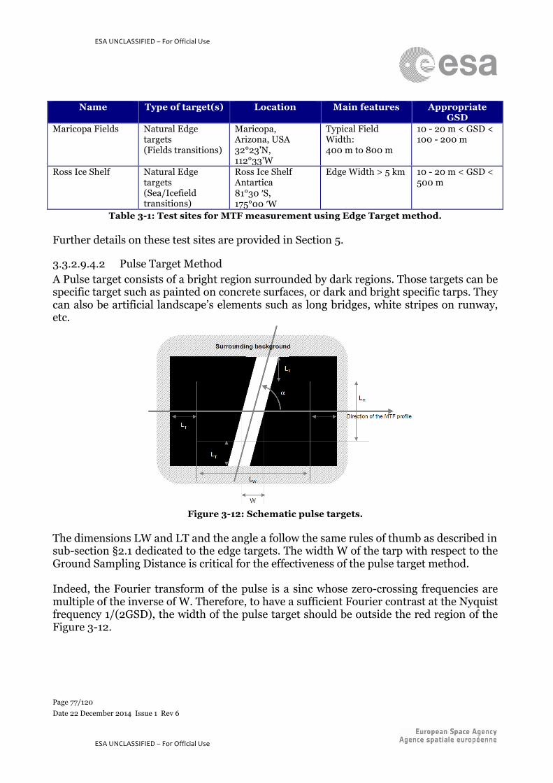
Page 77/120 Date 22 December 2014 Issue 1 Rev 6
ESA UNCLASSIFIED – For Official Use
ESA UNCLASSIFIED – For Official Use
Name Type of target(s) Location Main features Appropriate GSD
Maricopa Fields Natural Edge targets (Fields transitions)
Maricopa, Arizona, USA 32°23'N, 112°33'W
Typical Field Width: 400 m to 800 m
10 - 20 m < GSD < 100 - 200 m
Ross Ice Shelf Natural Edge targets (Sea/Icefield transitions)
Ross Ice Shelf Antartica 81°30 ′S, 175°00 ′W
Edge Width > 5 km 10 - 20 m < GSD < 500 m
Table 3-1: Test sites for MTF measurement using Edge Target method. Further details on these test sites are provided in Section 5.
3.3.2.9.4.2 Pulse Target Method A Pulse target consists of a bright region surrounded by dark regions. Those targets can be specific target such as painted on concrete surfaces, or dark and bright specific tarps. They can also be artificial landscape’s elements such as long bridges, white stripes on runway, etc.
Figure 3-12: Schematic pulse targets.
The dimensions LW and LT and the angle a follow the same rules of thumb as described in sub-section §2.1 dedicated to the edge targets. The width W of the tarp with respect to the Ground Sampling Distance is critical for the effectiveness of the pulse target method. Indeed, the Fourier transform of the pulse is a sinc whose zero-crossing frequencies are multiple of the inverse of W. Therefore, to have a sufficient Fourier contrast at the Nyquist frequency 1/(2GSD), the width of the pulse target should be outside the red region of the Figure 3-12.

Page 78/120 Date 22 December 2014 Issue 1 Rev 6
ESA UNCLASSIFIED – For Official Use
ESA UNCLASSIFIED – For Official Use
For sub-pixel pulse targets, the Fourier contrast at Nyquist frequency is high but the strength of the signal received by the sensor, linear with the width W, could be not enough for a good SNR budget. This fact can be circumvented by the selection of a very bright pulse target and/or a very large length target LH that would enables to stack a very large number of pulse responses to improve the SNR budget. In other cases, as stated by [Helder et al., 2004], a pulse width of 3 GSD ± 20 % is optimal (see Figure 3-13).
Figure 3-13: Fourier contrast of the W width pulse target at the Nyquist frequency.
The test sites for Sentinel-2 MTF measurement using this method are:
Name Type of target(s) Location Main features Appropriate GSD
Lake Ponchartrain Causeway
"Natural" Double Pulse target transitions)
Lake Ponchartrain Louisiana, U.S. 30°01'19"N, 90°09'14"W
Bridge width: 10 m Distance between bridges: 24.4 m CN ~ 1:4 (PAN)
5 - 10 m < GSD < 30 m
Bronx Whitestone Bridge
"Natural" Pulse target
Bronx Whitestone bridge, New York City, U.S. 40°48’05”N, 73°49’46”W
Bridge width: 26 m CN ~ 1:2 (PAN)
10 m < GSD < 60 m
Table 3-2: Test sites for MTF measurement using Pulse Target method. Further details on these test sites are provided in Section 5.

Page 79/120 Date 22 December 2014 Issue 1 Rev 6
ESA UNCLASSIFIED – For Official Use
ESA UNCLASSIFIED – For Official Use
3.3.3 Geometric Validation
3.3.3.1 Introduction The validation of the geometric performances will be performed on a yearly basis and will include:
o Geolocation uncertainty validation using reference sites with geometric patterns and for which geometry is mastered;
o Multi-temporal registration uncertainty validation using image correlation techniques;
o Multi-spectral registration uncertainty validation using correlation between images of different bands;
o Global Reference Images (GRI) Validation.
3.3.3.2 Geolocation Uncertainty Validation
3.3.3.2.1 Introduction The geolocation uncertainty is evaluated at two levels:
o System level, which are only dependent on the spacecraft configuration and without any improvement using auxiliary data (such as GCPs) or data processing.
o Product level, which quantify the uncertainty after geometric data processing (such as the refining of the viewing model).
The product level geolocation uncertainty is the one that will directly impact the users. Mission performance requirements (cf. section 1.9) validated by this activity are:
o S2-MP-100 (A priori absolute geolocation uncertainty) o S2-MP-105 (Absolute geolocation uncertainty without GCPs); o S2-MP-110 (Absolute geolocation uncertainty with GCPs).
3.3.3.2.2 System Level
3.3.3.2.2.1 Method Description This Activity is performed by MPC/ESL. This assessment is based on detection of ground control points by correlation with a database of accurately localised images spread over the world. These ground control points have to be more accurate than the targeted mission geolocation uncertainty, just as for the absolute calibration of viewing reference frames. T he quality of the measurement will depend on the uncertainty of the ground control points, their number and their distribution over the scene. One of the following methods is then used:

Page 80/120 Date 22 December 2014 Issue 1 Rev 6
ESA UNCLASSIFIED – For Official Use
ESA UNCLASSIFIED – For Official Use
Method 1 relies on the use of ground control points by estimating the location of these points on the ground (cf. Figure 3-14). For a given scene:
o Identification of an approximately large number of ground control points in the scene: (li, ci)à(xi, yi, hi)meas where i=(1,m).
o For each measured ground control point i, estimation of the location of this point on the ground (xi, yi)est using the location function;
o For each ground control point i, comparison of (xi, yi)est estimated terrain coordinates, with measured terrain coordinates (xi, yi)meas, which gives the location performance at this ground control point (dxi, dyi);
o Average location performance of the scene is then obtained by averaging the performance of the all ground control points in this scene.
(l,c)meas
F
(x,y)est
(x,y)meas
(dx,dy)h
Figure 3-14: Illustration of the method for estimating location performance in meters.
The estimation of performance is then directly in metres and accounts for all contributing factors. However, the estimate depends strongly on the ground control points quality. Method 2 involves no longer estimating location performance in metres on the ground, but in the focal plane. In this case, we use the inverse location function: from the GCP ground coordinates we estimate the image coordinates by means of the inverse geometric model and then compare them with measured image coordinates. Hence we obtain the location performance along rows (in pixels), also known as column location performance, and the location performance along columns (in pixels), also known as row location performance. The benefit of this method lies in obtaining the performance in the focal plane and therefore in better understanding the physical phenomena. Hence pitch, roll or yaw bias, magnification or even drift in pitch or roll, can be shown.
3.3.3.2.2.2 Inputs

Page 81/120 Date 22 December 2014 Issue 1 Rev 6
ESA UNCLASSIFIED – For Official Use
ESA UNCLASSIFIED – For Official Use
o Sentinel-2 acquisition needs are segments (spectral bands TBD), taken all over the world, including various latitudes and various seasons. These images are processed up to Level-1B without refinement.
o A database of very accurately localised images (with associated GCPs), located at various latitudes and longitudes, to correlate with the previous acquisitions.
3.3.3.2.2.3 Outputs A yearly report containing the output of geolocation performance measurement is the estimation of location in meters or roll, pitch, yaw biases in radians. The dependence of the geolocation evolution with the season or the latitude may also be analysed.
3.3.3.2.3 Product Level
3.3.3.2.3.1 Method Description This activity is performed by MPC/CC. Product performances, after refining and geometric processing, are verified over Level-1B product (geolocation or multispectral registration performance) or Level-1C product (multi-temporal registration). The objective is to characterize the geolocation performances of a Level-1B product, after refining over a well-geolocalised reference image. The geolocation performances at Level-1C are much alike, except the small error introduced by the resampling. This measure of performance uses the outputs of the space triangulation algorithm, stored in the Level-1B product metadata. Selected test sites are observed along the operational life of the satellite to detect any evolution of the sensors performance. As for geometric calibration, the global distribution of sites and various observation conditions is required in order to ensure good confidence in estimated performances. This method applies only to refined images.

Page 82/120 Date 22 December 2014 Issue 1 Rev 6
ESA UNCLASSIFIED – For Official Use
ESA UNCLASSIFIED – For Official Use
Level-‐1B RefinedMetadata
Residuals&
Refin. values
Geolocation Uncertainty
GeolocationPerformance
Expected refining values (GIPP)
Thresholds
Geolocation accuracy of GRI
Figure 3-15: Workflow of the Geolocation performance assessment.
1) The first step is to select only refined Level-1B products acquired over a given
period, thanks to the attribute of the tag <Image_Refining> present in the Level-1B product metadata. Most of the information needed for the computation of the geolocation in orbit can be found in the Level-1B product metadata. If the refining failed for a large percentage (threshold TBD) of products that have not been refined, a warning has to be raised and investigation has to take place about the cause of failure of the refining algorithm: attitude, orbit data can be faulty, or the images can be especially cloudy, etc. For each image, the algorithms verifies also that: o Image and ground spatiotriangulation residuals are null or very small (i.e.
below a reference threshold). o Roll, pitch and yaw biases (tag <Refined_Corrections_List><MSI_State>) are
smaller than the Level-1B processing parameters default values and eventually overwritten by the GIPP Parameters to be refined.
If this is not the case for a large percentage (Threshold TBD) of products, a similar warning has to be raised for fine investigation and maybe recalibration.
2) The following indicators are then computed:
o The geolocation uncertainty (planimetric and altimetric) after refining is the quadratic sum of the reference image geolocation root mean square uncertainty and the mean of root mean square deviation of the ground residuals for all the images.
o The geolocation uncertainty (planimetric and altimetric) before refining is the quadratic sum of the reference image geolocation RMS uncertainty, and the mean of RMS of the correlation residuals projected on ground.

Page 83/120 Date 22 December 2014 Issue 1 Rev 6
ESA UNCLASSIFIED – For Official Use
ESA UNCLASSIFIED – For Official Use
3.3.3.2.3.2 Inputs Sentinel-2 Level-1B products with refined geometric model and associated GIPPs. In order to be able to estimate geolocation accuracy, several input data are necessary:
a) Expected refining values, allowing to know the threshold of the refining values, b) Refining values of the geometrical models. c) Image and ground residuals of the spatiotriangulation and correlation residuals. d) Geolocation accuracy of the reference coverage.
a) These files contain the maximum (at 2σ) expected values for each correction re-estimated by the refining. Both files have to be taken into account: The file which contains the defaults values of the viewing model, which can be overwritten by the GIPP parameters to be refined. The viewing model configuration file contains the default maximum (at 2σ expected corrections for each Viewing Model State, given the on-board equipment precision. For example, if the GPS gives the position with a precision of 5m at 2σ confidence level, this value is indicated file for EVG state, and is used to compute a physically realistic position correction: this “maximum” value is used in the mean square regression algorithms, so as to constraint the correction on position within 5m. Alternatively, the GIPPs can be used so as to overwrite the indicated values of the processing chain configuration file. b) The Level-1B metadata contains all the results of the refining necessary to compute the geolocation performances indicators, under the datastrip level metadata tag <Geometric_Info>. The following tags are filled by the Level-1B processing: <RGM> Flag to identify if the Refined Geometric Model File is computed or obtained from an existing RGMF (reused) <Image_Refining> Contains the Refining results. If the refining has not been performed or has not succeeded, the output product shall be flagged “not refined”
<Refining_Characteristics> <Reference_Image_List>Reference images used for geometric model refining processing <Reference_band>The reference band is a spectral channel of the reference image. The geometric refining is performed using this channel
<VNIR_SWIR_Registration> Contains the VNIR_SWIR registration results. <Refined_Corrections_List>Description of the refined corrections. If the refining has been processed by datastrip then, there are the refined corrections for each datastrip.

Page 84/120 Date 22 December 2014 Issue 1 Rev 6
ESA UNCLASSIFIED – For Official Use
ESA UNCLASSIFIED – For Official Use
<Spacecraft_Position>Spacecraft position (expressed in meters) in the local spacecraft reference frame (EVG state) <MSI_State>MSI state (EIF state) <Focal_Plane_State> Focal plane state (EIM state)
c) The histogram of spatiotriangulation residual are to be found in the product metadata tag: <Quality_Assessment>
<Geometric_refining_quality> <Spatiotriangulation_Residual_Histogram>
It contains the image residuals and the ground residuals, and a large number of statistics associated to the histogram.
The tag <Quality_Assessment> <Geometric_refining_quality>
<Correlation_Residual_Histogram> contains image residuals found after correlation and a large number of statistics associated to this histogram.
d) The global RMS geolocation accuracy of the reference coverage is also needed. In fact, this reference coverage has been tightly localised during the on-board commissioning. However, it cannot be considered as perfect and its geolocation accuracy (both in planimetry and altimetry) has to be taken into account.
3.3.3.2.3.3 Outputs A 10-day periodicity report with MPI estimating the geolocation uncertainty after geometric processing. The indicators are giving a synthesis, either on a daily basis, or 10-days basis, over one cycle. The following indicators are to be computed:
o Planimetric and Altimetric geolocation accuracy of products before refining. o Planimetric and Altimetric geolocation accuracy of images after refining (Level-1B
products). o A warning indicating when the geometric GIPPs (biases in roll, pitch, yaw,
magnification or lines of sight) have to be recalibrated.
3.3.3.3 Multi-spectral Registration Uncertainty Validation
3.3.3.3.1 Introduction The multi-spectral registration consists in co-registering the various spectral bands among them in order to obtain a perfect stacking. The multi-spectral registration uncertainty is evaluated at two levels:

Page 85/120 Date 22 December 2014 Issue 1 Rev 6
ESA UNCLASSIFIED – For Official Use
ESA UNCLASSIFIED – For Official Use
o System level, which are only dependant on the spacecraft configuration and without any improvement using auxiliary data or data processing.
o Product level, which quantify the uncertainty after geometric data processing (such as the refining of the viewing model).
The mission performance requirement (cf. section 1.9) validated by this activity is S2-MP-120 (BOA reflectance uncertainty).
3.3.3.3.2 System Level
3.3.3.3.2.1 Method Description This method is performed by MPC/ESL. The goal of the multispectral registration assessment is to verify that the registration of spectral bands of images is within the specifications, with a special focus on the registration performance between the focal planes. This performance is computed before any geometric processing such as the focal plane registration of Level-1B processing. This performance is measured by correlation:
o Either directly as a side product of the relative focal plane calibration: the residuals of calibration give the multispectral registration performance;
o Either by additional correlations using a different band combination than the one used for the relative focal plane calibration, such as the correlation between B9 and B2, etc, so as to cross-check the performances. All the bands have to be correlated to at least a band of the other resolutions. It is not necessary to compute all the combinatory combinations between all spectral bands, but only a subset of combinations.
The image with the finest resolution is first resampled in the geometry of the images of the coarsest resolution, using the geometric model for resampling (the interpolation method will be at least B-spline). The correlation is then performed to collect tie points, and the shifts between the two images are filtered both in lines and columns. The multispectral registration value is directly deduced from the root mean square shift value, along lines or columns, between the two images. This value can also be expressed in distance (meters). Process can be performed through specific tools that are able to calculate correlation (e.g. cross-correlation, mutual information, feature detection and other image-matching techniques) between images and resulting performance parameters. Preliminary tests can take place to determine the best combination of bands for a successful correlation, due to radiometric contents of images. Band 10 may turn to be especially difficult to correlate with other bands, since it is radiometrically very different from other bands.

Page 86/120 Date 22 December 2014 Issue 1 Rev 6
ESA UNCLASSIFIED – For Official Use
ESA UNCLASSIFIED – For Official Use
3.3.3.3.2.2 Inputs The Sentinel-2 acquisition needs are images with all the spectral bands, at different dates and latitudes. These data are processed at Level-1B.
3.3.3.3.2.3 Outputs A 6-months periodicity report containing as main output is the multispectral registration performance expressed in pixels. Another output is the decision to enable the use of the registration between the two focal planes exceeds the specifications.
3.3.3.3.3 Product Level
3.3.3.3.3.1 Method Description This method is performed by both MPC/CC and MPC/ESL. The multi-spectral registration uncertainty may differ from the system multi-spectral registration uncertainty if the focal plane registration processing is enabled in the processing chain. The product performances within a focal plane are similar to the system performances when no refining is performed. The goal of the multispectral registration assessment is to verify that the registration of spectral bands of the two focal planes is within the specifications, after the registration performed by the Level-1B processing. This performance is measured:
o By the analysis of the registration outputs, such as the histograms of the spatiotriangulation;
o By additional correlations of bands in the two focal planes, such as B11/B5 or B12/B5, or B11/B4. In this case, the image with the finest resolution is first resampled in the geometry of the images of the coarsest resolution, using the geometric model for resampling.
The correlation is then performed to collect tie points, and the shifts between the two images are filtered both in lines and columns. The multispectral registration value is directly deduced from the root mean square shift value, along lines or columns, between the two images. This value can also be expressed in distance (meters). Process can be performed through specific tools that are able to calculate correlation (e.g. cross-correlation, mutual information, feature detection and other image-matching techniques) between images and resulting performance parameters.
3.3.3.3.3.2 Inputs Level-1B products with following optional processing performed:
o Only “registration”. o Both “registration” and “refining”.

Page 87/120 Date 22 December 2014 Issue 1 Rev 6
ESA UNCLASSIFIED – For Official Use
ESA UNCLASSIFIED – For Official Use
3.3.3.3.3.3 Outputs A cyclic (10 day) periodicity report by MPC/CC and a 6-month periodicity report by MPC/ESL containing MPI evaluating the multi-spectral registration uncertainty between VNIR and SWIR focal planes.
3.3.3.4 Multi-Temporal Registration Uncertainty Validation
3.3.3.4.1 Introduction The objective is to characterise the multi-temporal registration of the Level-1C tiles, after geometric processing. The mission performance requirement (cf. section 1.9) validated by this activity is S2-MP-115 (Multi-temporal registration).
3.3.3.4.2 Method Description This method is implemented both by MPC/CC and MPC/ESL. The multi-temporal performances are measured, per band, starting from Level-1C tiles using correlation technique, without resampling, since it is done in a given cartographic projection. This relative measurement is important to appreciate stability of the instrument, to distinguish year-to-year and season-to-season variations due to global change from technical issues that may arise during operations. The method relies on image-matching technique that depends on the matching factor. It is important to note that the matching factor reflects the quality of the image matching procedure. Various factors influences the matching factor, some are listed just here after:
• The quality of the images, • The seasonal variation and meteorological / atmospheric properties, • The properties of the terrain, relief, surface reflectance, and information content, • The similarities of spectral bands (in case of different cross comparison).
The seasonal variation and especially the atmospheric properties at the time of observation are key parameter for image-to-image registration. Any configuration that limits the water vapour is more suitable; arid regions, winter season. In addition, aerosols may be limited using an elevated test field (above 1000 m), As all geometric uncertainties measured by correlation, this estimate is pessimistic since the homologous points or ground control points are not perfectly localised, an error is associated to these ground control points.

Page 88/120 Date 22 December 2014 Issue 1 Rev 6
ESA UNCLASSIFIED – For Official Use
ESA UNCLASSIFIED – For Official Use
3.3.3.4.3 Inputs A set of temporal series of Level-1C tiles over different areas around the world.
3.3.3.4.4 Outputs A cyclic (10 day) periodicity report by MPC/CC and a 6-month periodicity report by MPC/ESL containing MPI evaluating the multi-temporal registration uncertainty.
3.3.3.5 Global Reference Images Validation
3.3.3.5.1 Introduction The GRI validation approach is based on the same method used for the GRI Quality Assessment (cf. section 3.2.3.3.1.2.6).
3.3.3.5.2 Method Description The GRI validation will be performed by the analysis of the spatiotriangulation outputs. An estimation of the overall geo-location error budget is computed, considering:
• The residual error estimated on each point after the refining shall be as small as possible;
• An external source of GCP (not used for refining). The process of determining the spatiotriangulation residuals (for the first case) or the distances between the GRI and the GCPs (for the second case) will introduce an error (mainly due to the correlation technique). Assuming that this error will be spatially random and the number of TPs/GCPs is sufficiently high, it can be assumed that it will be averaged out and can be considered negligible. Estimating the representativity of the solution found by the mean square optimisation can also assess the achieved quality. If the corrections estimated by the algorithm exceed a given pre-defined threshold (defined from the absolute geo-location error specified), the GRI image is considered not valid. This method will be defined in detail by the MPC consortium.
3.3.3.5.3 Inputs The GRI and reference Ground Control Points (GCPs) not used for the refining process.
3.3.3.5.4 Outputs A 1-year periodicity report by MPC/ESL containing MPI evaluating the GRI geolocation accuracy and completeness.

Page 89/120 Date 22 December 2014 Issue 1 Rev 6
ESA UNCLASSIFIED – For Official Use
ESA UNCLASSIFIED – For Official Use
4 LEVEL-2A
4.1 Introduction This chapter provides a high-level overview of the calibration and validation activities that will be carried on the Level-2A algorithms and products.
4.2 Level-2A Calibration For Cloud Screening, algorithms will be calibrated (i.e. threshold and parameters will be defined) based on an empirical approach using an imagery dataset composed by a calibration sub-set (for defining the algorithm parameters) and a validation sub-set (for algorithm and products validation purposes). For Atmospheric Correction, the calibration of the algorithms and the validation of the obtained products (bottom-of-atmosphere reflectance, aerosol optical thickness and water vapour content) will be performed using a set of test sites representative of main surface-atmosphere types. Level-2A calibration activities will be defined in detail by the MPC consortium.
4.3 Level-2A Validation Most of the time, the atmospheric correction is a derived product from the aerosol remote sensing. Therefore, the validation of the atmospheric correction is often limited to the validation of the aerosol product. Validation of the surface reflectance is a difficult task, which needs first to combine at the time of overpass a representative sampling of the surface reflectance at the pixel size. It also needs to account for the difference in geometry between satellite and ground based measurements. On a practical point of view a validation strategy is relevant for high spatial resolution sensors like MSI which allows collecting representative samples of the surface reflectance at nadir, which is the common view geometry of high spatial resolution sensors. One difficulty with this validation is for heterogeneous surface is the contamination by the so-called adjacency effects. The mission performance requirement (cf. section 1.9) validated by this activity is S2-MP-200 (Uncertainty of the bottom-of-atmosphere reflectance). Level-2A validation activities will be defined in detail by the MPC consortium.

Page 90/120 Date 22 December 2014 Issue 1 Rev 6
ESA UNCLASSIFIED – For Official Use
ESA UNCLASSIFIED – For Official Use
5 ANNEX A: CALIBRATION AND VALIDATION TEST SITES
5.1 Introduction Table 5-1 provides an overview of the test sites that could be used for the calibration and validation activities of Sentinel-2. Following chapters provide a description of each test site. Test Site Level-1
Radiometric Calibration
Level-1 Radiometric Validation
Level-1 Geometric Calibration
Level-1 Geometric Validation
Level-2A Calibration
Level-2A Validation
Tuz Gölü √ √ Dome-C √ √ La Crau √ √ √ Barrax √ √ √ √ √ Greenland √ Table 5-1: List of Sentinel-2 calibration and validation test sites and associated purpose.
5.2 CEOS Test Sites For a quantitative validation, these sites will include the RADCALNET sites which are a set of Land Equipped Sites (LES) endorsed by CEOS as standard reference sites for the calibration of space-based optical imaging sensors. In addition, ad-hoc validation campaigns will be organized involving airborne, balloon and ground measurements. Further information on the mentioned test sites and the CEOS cal/val activities can be found at the Cal/Val Portal (http://calvalportal.ceos.org/ ). Following sections provide a description of the LES that could be used for Sentinel-2 Cal/Val activities.
5.2.1 Frenchman Flat (USA)
5.2.1.1 Overview The LSpec vicarious calibration site is situated on a homogeneous section of the Frenchman Flat dry lakebed found North-North-East of Mercury, Nevada on the Nevada Test Site (NTS) range. Center coordinates for the instrumented area are 115.93479 West longitude and 36.80928 North latitude. This playa is not unique for this application; vicarious calibration campaigns have been conducted over a variety of playa scattered throughout the Southwest. The Frenchman Flat playa surface is hard and clay-based. It has proven an ideal site with respect to surface homogeneity, restricted access (useful to eliminate vandalism), and infrastructure courtesy of the Non-Proliferation Testing and Evaluation Center (NPTEC). The NPTEC staff provides assistance with respect to site access and clearing, storage,

Page 91/120 Date 22 December 2014 Issue 1 Rev 6
ESA UNCLASSIFIED – For Official Use
ESA UNCLASSIFIED – For Official Use
communications, and the comforts of indoor office space. Data from the LSpec in-situ instruments are uploaded to the processing site at JPL. Communications are provided via a local cell tower. In comparing this site to Railroad Valley, a commonly used playa, we note that Railroad Valley is an ideal site for sensors up to several kilometres in extent; Frenchman Flat supports sensors with footprints less than 300 m. The disadvantages of Railroad Valley are its remote location and lack of infrastructure, including access to a cell tower for the data upload. The surface contains more loose sand and salts and is therefore less stable.
5.2.1.2 Instruments on the Test Site o LED Pods o Cimel Automatic Sun Tracking Photometer CE 318 o ASD campaign radiometer o PARABOLA o Meteorological observations
5.2.2 La Crau (France)
5.2.2.1 Overview The La Crau test site is located in southeastern France at 4.87°E longitude and 43.50°N latitude about 50 km northwest of Marseille. It is a flat area of about 60 km2. The ground is uniformly covered by pebbles and dry grass-like vegetation. From a certain distance the ground looks like a homogeneous flat surface of a yellowish, brownish colour tone. The climate in this region is dry and sunny and the optical properties of the ground vary little during the year. For the calibration a section of 400 x 400 m2 in the center of the test site is used. This center section is called the calibration area
5.2.2.2 Absolute Radiometric Calibration The La Crau test site was used on routine basis for SPOT calibration. Therefore it is equipped with a CIMEL automatic radiometer operated by the CNRS LISE French laboratory originally developed for SPOT absolute radiometric calibration. The instrument is a sunphotometer mounted on a 10 meter high mast and consists of two collimators, one for IR channels (Germanium detector) and one for visible bands (Silicon detector). The instrument delivers data in nine spectral bands 10 nm wide. The central wavelengths are 380 nm for molecular scattering, 440 nm, 550 nm, 670 nm, 870 nm and 1600 nm for aerosols in the SPOT and VEGETATION spectral bands, 936 nm for the water vapour, 1020 nm to complete the aerosols knowledge. The radiance at 870 nm is acquired both

Page 92/120 Date 22 December 2014 Issue 1 Rev 6
ESA UNCLASSIFIED – For Official Use
ESA UNCLASSIFIED – For Official Use
with the IR and the visible collimators in order to intercalibrate them. The automatic operating procedure includes 3 sequential modes repeated all the day long for optical airmasses up to 5. In the first mode, the sun collimator points at the sun and measures direct solar irradiance in order to retrieve the water vapour abundance, aerosol optical depths and the Angström coefficient. The second mode consists in sky radiances measurements in the almucantar and principal plane and is used for phase function retrieval. In the last mode, the collimator scans the ground both in azimuthal and zenital directions and measures the surface BRDF. This instrumentation enables autonomous self-sufficient measurements for SPOT calibration.
5.2.2.3 Geometric Calibration This test site is devoted to sensor geometry calibration. Site Name Number
of GCPs GCP Collection
Method Location (lat,long)
Altitude Range (m)
Calibration Parameters
Site Coverage (NSxEW)
La Crau (France)
35 -DGPS -DEM (Spot)
46.839 N 7.533 W
[0-200] MSI exterior and interior orientation, and direct location
20 km x 20 km
5.2.3 Dome-C (Antarctica)
5.2.3.1 Overview Dome C is a French-Italian scientific station located on the East Antarctic ice sheet. The altitude of the site is 3215 m and the distances from the coasts are larger than 1000 Km. Site is located at -74.50 latitude and +123.00 longitude. It is one of the CEOS RADCALNET Sites. The site is managed by France and Italy (Dc is directed by French Polar Institute (IPEV) and Italian polar Institute (ENEA).
5.3 Other Test Sites
5.3.1 Barrax (Spain) Barrax test site is located in South-East Spain 20 km from the Albacete (coordinates 30°3’ N, 2° 6’ W). The area is characterised by a flat morphology and large, uniform land-use units. Differences in elevation range up to 2 m only. The regional water table is about 20-30 m below the land surface.

Page 93/120 Date 22 December 2014 Issue 1 Rev 6
ESA UNCLASSIFIED – For Official Use
ESA UNCLASSIFIED – For Official Use
The climatic conditions accord the Mediterranean features: high precipitations in spring and autumn and the minimum in summer. The annual rainfall averages is about 400 mm. Furthermore, the region has high continentally with high thermal oscillations during all seasons. La Mancha represents one of the driest regions of Europe. The region consists of approximately 65% dry land and 35% irrigated land with different agricultural fruits. The test area has the following co-ordinates (related to UTM, Zone 30, DATUM WGS84): Geographical corner coordinates:
o Corner 1: 575505.9523E 4323210.7146N o Corner 2: 585226.6519E 4325555.7469N o Corner 3: 575039.5028E 4325144.3194N o Corner 4: 584760.2034E 4327489.3472N
5.3.2 Maricopa Fields (USA) This test site is suited for MTF validation.
Name Type of target(s) Location Main features Appropriate GSD
Maricopa Fields Natural Edge targets (Fields transitions)
Maricopa, Arizona, USA 32°23'N, 112°33'W
Typical Field Width: 400 m to 800 m
10 - 20 m < GSD < 100 - 200 m
5.3.3 Ross Ice Shelf (Antarctica) This test site is suited for MTF validation.
Name Type of target(s) Location Main features Appropriate GSD
Ross Ice Shelf Natural Edge targets (Sea/Icefield transitions)
Ross Ice Shelf Antartica 81°30 ′S, 175°00 ′W
Edge Width > 5 km 10 - 20 m < GSD < 500 m
5.3.4 Lake Ponchartrain Causeway (USA) This test site is suited for MTF validation.
Name Type of target(s) Location Main features Appropriate GSD

Page 94/120 Date 22 December 2014 Issue 1 Rev 6
ESA UNCLASSIFIED – For Official Use
ESA UNCLASSIFIED – For Official Use
Lake Ponchartrain Causeway
"Natural" Double Pulse targettransitions)
Lake Ponchartrain Louisiana, U.S. 30°01'19"N, 90°09'14"W
Bridge width: 10 m Distance between bridges: 24.4 m CN ~ 1:4 (PAN)
5 - 10 m < GSD < 30 m
5.3.5 Bronx Whitestone Bridge (USA) This test site is suited for MTF validation.
Name Type of target(s) Location Main features Appropriate GSD
Bronx Whitestone Bridge
"Natural" Pulse target
Bronx Whitestone bridge, New York City, U.S. 40°48’05”N, 73°49’46”W
Bridge width: 26 m CN ~ 1:2 (PAN)
10 m < GSD < 60 m
5.3.6 Manosque (France) This test site is suited for sensor geometry calibration. Site Name Number
of GCPs GCP Collection
Method Location (lat,long)
Altitude Range (m)
Calibration Parameters
Site Coverage (NSxEW)
Manosque (France)
TBC -Large Scale aerial photography (PELICAN) – GSD Resolution 50 cm -DSM – IGN BDZ Resolution 1m
43.499 N 5.479 E
[200-600] MSI interior orientation
30 km x 60 km
5.3.7 Bern/Thun (Switzerland) This test site is suited for sensor geometry calibration. Site Name Number
of GCPs GCP Collection
Method Location (lat,long)
Altitude Range (m)
Calibration Parameters
Site Coverage (NSxEW)
Bern/Thun (Switzerland)
138 -DGPS -DSM (from Aerial Photo)
46.839 N 7.533 E
[500-1250] MSI exterior and interior orientation
3 zones: -Bern: 110 km2 -Thun: 100 km2 -Southwest: 90 km2

Page 95/120 Date 22 December 2014 Issue 1 Rev 6
ESA UNCLASSIFIED – For Official Use
ESA UNCLASSIFIED – For Official Use
5.3.8 Cape Town (South Africa) This test site is suited for sensor geometry calibration. Site Name Number
of GCPs GCP Collection
Method Location (lat,long)
Altitude Range (m)
Calibration Parameters
Site Coverage (NSxEW)
Cape Town (South Africa)
35 Existing data – IKONOS
33.99 S 18.75 E
[23-70] Direct location
70 km x 70 km

Page 96/120 Date 22 December 2014 Issue 1 Rev 6
ESA UNCLASSIFIED – For Official Use
ESA UNCLASSIFIED – For Official Use
6 ANNEX B: CALIBRATION AND VALIDATION COMPLEMENTARY METHODS DESCRIPTION
6.1 Method for the Update of Pixel Status
6.1.1 Background Once in flight, the Sentinel-2 pixel status will need to be confirmed, checking eventual pixel response anomalies that might degrade the SNR level.
6.1.2 Objective The goal of this section is to describe a method for updating the pixel status using the SNR values estimated with the sun diffuser calibration measurements.
6.1.3 Inputs The entry data needed for the SWIR pixel selection are:
o SNR(p,b,d), a line of SNR for each detector and band calculated using a calibration acquisitions (dark signal and sun diffuser).
o DC(p,b,d), a line of the mean digital count on a diffuser image. o RP_Bj_ST_Di (from the [ICCDB]) used for initializing the pixel status vector
Pstatus(k,p,b,d). o SNRspec(b), the SNR defined in the Sentinel-2 initial specification (cf. S2-MP-035). o SNRmin(b), the SNR acceptable for the mission. o SNRmax(b), a threshold SNR allowing to identify an infinite SNR due to pixel
saturation. o DCmin(b), the minimum digital count for a non-blind pixel. o DCmax(b), the maximum digital count for a non-saturated pixel.
6.1.4 Outputs o Pstatus(k,p,b,d), pixel status for each pixel “p”, band “b” and detector module “d”.
Index k=0 indicates that this status corresponds to the combined photo-sensitive lines response, values greater than 0 would correspond to each single photo-sensitive line status (applicable only for SWIR bands).
6.1.5 Method Description The goal of this first step is to evaluate the quality of the pixels of the SWIR detectors and check if the SNR specifications are met. The SNR is calculated following specifications described in [MSI-CCIF] and based on calibration acquisitions (sun diffuser and dark signal). This value is also required for the SNR Validation activity (Section 3.3.2.7).

Page 97/120 Date 22 December 2014 Issue 1 Rev 6
ESA UNCLASSIFIED – For Official Use
ESA UNCLASSIFIED – For Official Use
Seven pixel status are defined as Pstatus(k,p,b,d) of photo-sensitive line(s) “k”, pixel “p”, band “b” and detector “d”:
o 1: operational pixel with SNR compliant to specification; o 2: operational pixel with SNR below specification; o 3: non-operational saturated pixel; o 4: non-operational blind pixel; o 5: non-operational with SNR below specification; o 3bis: non-operational saturated pixel with status to be confirmed; o 4bis: non-operational blind pixel with status to be confirmed.
The first four statuses are the same as in the ICCDB. Pstatus(k,p,b,d) is initialized at the beginning of the operational phase (Mission Phase-E2) considering the health status vector RP_Bj_ST_Di from the ICCDB [ICCDB-ICD][ICCDB]. For each detector “d” of the 12 detectors,
For each band “b” of the 13 spectral bands, For each pixel “p”,
If SNR(p,b,d) > SNRspec(b) AND SNR(p,b,d) < SNRmax(b) Pstatus(0,p,b,d)=1 (No change. The pixel satisfies the SNR specification) End If SNR(p,b,d) > SNRmax(b) AND DC(p,b,d) < DCmin(b) Pstatus(0,p,b,d)=4 (The SNR is infinite because the pixel is blind) End If SNR(p,b,d) > SNRmax(b) AND DC(p,b,d) > DCmax(b) Pstatus(0,p,b,d)=3 (The SNR is infinite because the pixel is saturated) End If SNR(p,b,d) < SNRspec(b) AND SNR(p,b,d) > SNRmin(b) Pstatus(0,p,b,d)=2 (The pixel is noisy but still operational) End If SNR(p,b,d) < SNRmin(b) Pstatus(0,p,b,d)=5 (The pixel is too noisy to be operational) End
End End
End Where SNR(p,b,d) is the value of the SNR for the pixel p and DC(p) is the digital count of the pixel p. For B10, the status of the selected line “k” Pstatus(k,p,b,d) takes the value of the overall status Pstatus(0,p,b,d).

Page 98/120 Date 22 December 2014 Issue 1 Rev 6
ESA UNCLASSIFIED – For Official Use
ESA UNCLASSIFIED – For Official Use
For B11 and the B12 bands, the analysis of the SNR only gives information on the group of selected pixels and not on the pixels separately. Therefore, the Pstatus(0,p,b,d) shall be changed to the status 3bis or 4bis and will be updated after the next acquisition on the sun diffuser, which will provide more information using different selected pixels.
6.2 Method for SWIR Detectors Re-arrangement Parameters Generation
6.2.1 Background The Sentinel-2 MSI SWIR focal plane covers 3 spectral bands B10, B11 and B12 respectively centred at 1375 nm, 1610 nm and 2190 nm [OCD]. The overall focal plane is made of 12 detectors to cover the full swath of Sentinel-2. The B10 detectors is made of three lines (with 1296 columns) with only one photosensitive line whereas the B11 and B12 detectors are made of four lines (with 1296 columns) with two consecutive photosensitive lines for the TDI mode (Figure 6-1).
Figure 6-1: Illustration of the focal plane.
After ground characterisation, for each of the 12 detector modules and each of these SWIR spectral bands, a vector RP_Bj_ST_Di(k,p,b,d), provides the health status of each pixel of the detector module, where Bj is the spectral band j, i is the detector module number (between 1 and 12) and k is the index of the selectable line (between 1 and Nj, number of selectable lines for each band) [ICCDB-ICD][ICCDB]. Four values are possible for each pixel:
o 1: operational pixel with SNR compliant to specification; o 2: operational pixel with SNR below specification; o 3: non-operational saturated pixel; o 4: non-operational blind pixel.

Page 99/120 Date 22 December 2014 Issue 1 Rev 6
ESA UNCLASSIFIED – For Official Use
ESA UNCLASSIFIED – For Official Use
The combined SNR of the SWIR photo-sensitive lines is estimated as part of the in-flight validation activities using calibration acquisitions (dark signal and sun diffuser). This information is stored in the Pstatus(k,p,b,d) (cf. section 6.1). For each of the 1296 columns and for each of the eleven lines implemented on the SWIR detector, a flag is set to zero if the related pixel is not selected and set to 1 if the pixel is selected for being used during acquisitions. The statuses of all the pixels and the choice of the selected one are initialised at ground level and they are updated according to the pixel status (which is related to the measured SNR level).
6.2.2 Objective The goal of this method is to describe the method to update the SWIR detectors configuration according to an updated pixel status vector.
6.2.3 Inputs The entry data needed for the SWIR pixel selection are:
o Pstatus(k,p,b,d), pixel status for each band “b” and detector module “d”. Index “k” equal to zero corresponds to the total combined pixel status. Values greater than zero point to the individual photo-sensitive lines for SWIR bands.
o S(p,b,d), a two dimensional vector indicating the SWIR pixels configuration for the operational production.
o SNRground(k,p,b,d), on-ground measured SNR for each line (for SWIR bands), pixel, band and detector module. Derived from [ICCDB] pre-flight data.
o A line of SNR for each detector of the SWIR spectral bands (B10, B11 and B12). o All inputs required for performing the “Method for the Update of Pixel Status” (cf.
section 6.1).
6.2.4 Outputs o Supdated(p,b,d), a new version of the pixels configuration for the operational
production of the three spectral bands B10, B11 and B12 (SWIR_pixels_configuration).
o Pstatus(k,p,b,d), updated pixel status.
6.2.5 Method Description For all the selected pixels, if the current pixel status Pstatus(0,p,b,d) is different from 1 or 2, then new selected pixels shall be chosen for the operational mode.

Page 100/120 Date 22 December 2014 Issue 1 Rev 6
ESA UNCLASSIFIED – For Official Use
ESA UNCLASSIFIED – For Official Use
6.2.5.1 Case B10 For the spectral band B10, one of the two others non-selected but operational pixels shall be chosen. If the two others pixels are operational (status 1 or 2), then the pixel with the higher ground SNR (SNRground) will be selected instead of the defective pixel. If only one pixel left is operational then, this pixel will be the new selected one. If none of the two other pixels fills these conditions, then, there will be no operational pixel in this position and the value of the pixel shall be interpolated in the image, using the neighbourhood pixels.
6.2.5.2 Case B11 and B12 For the spectral bands B11 and B12, the constraints are different because the two pixels that are selected must be consecutive (due to the TDI mode) and the SNR only give us an information on the two pixels “together” and not on the pixels separately. Therefore, different cases must be listed depending on the position of the selected pixels and on the status obtained during the first step of this processing and the ground status of the two other pixels. Considering Supdated the new selected pixels for the operational mode, then: Case 1: The selected pixels before processing are located line 1 and 2 S(p,b,d)=(1,2): If S(p,b,d)= (1,2)
If (Pstatus(3,p,b,d) and Pstatus(4,p,b,d)) = 1 or 2 Then Supdated(p,b,d)=(3,4)
End If (Pstatus(3,p,b,d) = 1 or 2) AND (Pstatus(4,p,b,d) != 1 or 2)
Then Supdated(p,b,d)=(2,3) If after a new SNR measurement and update of the pixel status (cf. section 6.1), Pstatus(0,p,b,d) = 1 or 2
Then the choice is confirmed and if Pstatus(1, p,b,d)= 4bis then Pstatus(1,p,b,d)= 4 if Pstatus(1, p,b,d)= 3bis then Pstatus(1,p,b,d)=3
End If (Pstatus(3,p,b,d) and Pstatus(4,p,b,d)) = 3 or 4
Then, no solution for this pixel. The radiance will be interpolated using the neighbourhood pixels.
End End Case 2: The selected pixels before processing are located line 2 and 3 S(p,b,d)=(2,3):

Page 101/120 Date 22 December 2014 Issue 1 Rev 6
ESA UNCLASSIFIED – For Official Use
ESA UNCLASSIFIED – For Official Use
This case is the more complex, as only some tests with new acquisitions will allow us to choose another couple of pixels. If S(p,b,d)= (2,3)
If (Pstatus(1,p,b,d) and Pstatus(4,p,b,d)) = 1 or 2 if SNRground(1,p,b,d) > SNRground(4,p,b,d) Then Supdated(p,b,d)= (1,2) If after a new SNR measurement and update of the pixel status (cf. section 6.1), Pstatus(0,p,b,d) = 1 or 2
Then the choice is confirmed and if Pstatus(3, p,b,d)= 4bis then Pstatus(3, p,b,d)= 4 if Pstatus(3, p,b,d) = 3bis then Pstatus(3, p,b,d)=3
Else Then Supdated = (3,4) If after a new SNR measurement and update of the pixel status, Pstatus(0,p,b,d) = 1 or 2
Then the choice is confirmed and if Pstatus(2, p,b,d)= 4bis then Pstatus(2, p,b,d)= 4 if Pstatus(2, p,b,d) = 3bis then Pstatus(2, p,b,d)=3
If (Pstatus(1,p,b,d) and Pstatus(4,p,b,d)) = 3 or 4 Then, no solution for this pixel. The radiance will be interpolated using the neighbourhood pixels.
End End Case 3: The selected pixels before processing are located line 3 and 4 S(p,b,d)=(3,4): If S(p,b,d)= (3,4)
If (Pstatus(1,p,b,d) and Pstatus(2,p,b,d)) = 1 or 2 Then Supdated = (1,2)
End If (Pstatus(2,p,b,d) = 1 or 2) AND (Pstatus(1,p,b,d) != 1 or 2)
Then Supdated = (2,3) If after a new SNR measurement and update of the pixel status (cf. section 6.1), Pstatus(0,p,b,d) = 1 or 2
Then the choice is confirmed and if Pstatus(4, p,b,d)= 4bis then Pstatus(4,p,b,d)= 4 if Pstatus(4, p,b,d)= 3bis then Pstatus(4,p,b,d)=3
End If (Pstatus(1,p,b,d) and Pstatus(2,p,b,d)) = 3 or 4
Then, no solution for this pixel. The radiance will be interpolated using the neighbourhood pixels.
End End

Page 102/120 Date 22 December 2014 Issue 1 Rev 6
ESA UNCLASSIFIED – For Official Use
ESA UNCLASSIFIED – For Official Use
6.3 Method for Dark Signal and Pixel Contextual Offset Correction
6.3.1 Background Dark signal and pixel contextual offset corrections are applied during Level-1 processing as part of the systematic radiometric corrections of Level-1B (according to Eq. 7 and Eq. 8). The correction is also necessary when processing calibration data.
6.3.2 Objective The goal of this method is to perform dark signal and pixel contextual offset correction. This function shall be modular enough to allow for:
o Dark signal non-uniformity correction only (PCmasked is not considered). o Full correction (DS and PCmasked are both corrected).
It shall be possible:
o To apply the dark signal and pixel contextual offset correction to an image or a region of an image, saving the result on disk.
o To apply the correction to a data buffer (a region or a line loaded in memory) in view of reuse and integration in other programs (for instance when computing the absolute calibration coefficients).
6.3.3 Inputs o Level-0 product. o DS coefficients and PCmasked parameters. o Flags to enable/disable separately the dark signal and the pixel contextual offset
correction. o First and last line of the region to be processed. o Band number, line number if applied on a single line/band.
6.3.4 Outputs o Dark signal corrected image/region/buffer depending on input.
6.3.5 Method Description
If requested, compute PCmasked according to Eq. 8.
Compute Y = X - DS - PCmasked with DS or PCmasked set to zero if indicated in input

Page 103/120 Date 22 December 2014 Issue 1 Rev 6
ESA UNCLASSIFIED – For Official Use
ESA UNCLASSIFIED – For Official Use
parameters.
6.4 Method for Diffuser Geometry Modelling
6.4.1 Background The relative gains calibration (section 3.2.2.5.2) and the absolute radiometric calibration (section 3.2.2.5.3) require the calculation of the MSI on-board sun diffuser geometry. Modelling the geometry of the acquisition is necessary to determine the solar and viewing angles on the diffuser surface (θsd, 𝜙sd , θv, 𝜙v) and thus calculate the radiance seen by the instrument.
6.4.2 Objective The goal of this method is to determine the geometry of the diffuser. The solar angles θsd and 𝜙sd are retrieved for each line of the input data. The viewing angles θv and 𝜙v are retrieved for each pixel of each line of the input data for all the detectors and the spectral bands. Figure 6-2 illustrates the geometry of the diffuser surface with respect to the instrument and to the sun.
Figure 6-2: Diffuser geometry.
6.4.3 Inputs The Level-0 product is composed of two parts: the metadata and the image data. The product metadata holds the ancillary data pertinent to the acquisition:

Page 104/120 Date 22 December 2014 Issue 1 Rev 6
ESA UNCLASSIFIED – For Official Use
ESA UNCLASSIFIED – For Official Use
o Start time of the acquisition for each detector. o GPS position and velocities in WGS84. o AOCS corrected attitudes in J2000. o IERS bulletin for the acquisition date (pole coordinates, UT1-UTC).
Processing parameters:
o GIPP «Viewing Directions» defining the directions tan ψx and tan ψx for each pixel of each detector d and band b.
o GIPP «Spacecraft Model» defining the transformations matrices from the MSI reference frame to the focal plane, and to the detector frames.
o The GICP that defines in which calibration mode is the diffuser: nominal or redundant (defined in the ancillary data).
o Diffuser model: - Transformation matrices from the Piloting reference frame to the diffuser
(PRF->DIF). - Stray-light correction coefficients for each spectral band. - BRDF model (analytic model or ground measurements plus interpolation
filter). o The GIPP « Blind pixels » which contains the list of blind pixels.
6.4.4 Outputs o Solar angles for each line of the scene. o Viewing angles for each pixel of each line and each band (13 bands, full image). o Reflectance of the diffuser for each viewing angle.
6.4.5 Method Description The Level-0 image data, once uncompressed, is made of the raw digital counts recorded by the instrument. For multi-lines detectors, only the selected pixels remain such that the output may be considered as if the detectors were single-line detectors. The viewing directions give the viewing directions of the selected pixels only. In calibration mode, no equalization is applied by the WICOM on board. The rearrangement of the pixels for band B11 and B12 is not performed. The process is applied to a region of the product defined by the first and last line numbers to be extracted. The radiance observed on the diffuser is dependent on the viewing and solar geometry. In order to determine the angles θsd, 𝜙sd, θv, 𝜙v we need to model the geometry of the diffuser. A function to compute the solar and viewing angles on the diffuser shall be implemented. The solar angles θsd, 𝜙sd shall be retrieved for each line of the input data. The viewing angles θv and 𝜙v shall be retrieved for each pixel, detector and band of each line of the

Page 105/120 Date 22 December 2014 Issue 1 Rev 6
ESA UNCLASSIFIED – For Official Use
ESA UNCLASSIFIED – For Official Use
input data. θv, 𝜙v vary with the pixel/detector/band but not with time as the position of the diffuser is fixed with respect to the instrument. θv, 𝜙v is therefore constant for each line of the image. Viewing directions in the diffuser frame The viewing angles in the diffuser frame are provided within the [ICCDB]. Only in case the provided values are considered not precise enough, the viewing directions in the diffuser frame shall be computed for each pixel/band/detector in the diffuser reference frame. The steps are described below.
1. The GIPP Viewing directions gives the direction of each pixel in the reference frame of the detector and band it belongs to, referenced as (B,D). The viewing directions V!
are described in terms of the two angles ψx and ψy such as
VB,D (p,b) =
⎟⎟⎟
⎠
⎞
⎜⎜⎜
⎝
⎛
−
1tantan
x
y
ψ
ψ.
2. The viewing vector is converted in the piloting reference frame according to the equation:
VPRF =MMSI−>PRFMVNIR−>MSIM (B,D)−>VNIR
V(B,D) for the VNIR bands, and
),(),( DBSWIRDBMSISWIRPRFMSIPRF VMMMV!!
>−>−>−= for the SWIR. The GIPP “spacecraft model parameters” gives the transformations from PRF to (B,D) as a series of rotation and scales (cf. (see §3.2.3 and §4 of [GPP-ATBD-VM]). The direction must be inverted to determine the matrices PRFMSIM >− , MSISWIRM >− and
SWIRDBM >−),( . The labels VNIR and SWIR refer to the reference frames of the VNIR and SWIR focal planes.
3. The viewing directions are then computed in the diffuser frame according to the transformation given in the GIPP Diffuser Model:
PRFDIFPRFDIF VMV!!
>−=
From ⎟⎟⎟
⎠
⎞
⎜⎜⎜
⎝
⎛
=
VzVyVx
VDIF!
we deduce the viewing angles θv, ϕv:
𝜃! = 𝑎𝑟𝑐𝑐𝑜𝑠 −𝑉! 𝜙! = −𝑎𝑟𝑐𝑡𝑎𝑛2 −𝑉! ,−𝑉!
Sun direction in the diffuser frame

Page 106/120 Date 22 December 2014 Issue 1 Rev 6
ESA UNCLASSIFIED – For Official Use
ESA UNCLASSIFIED – For Official Use
The computation of the solar angles in the diffuser frame first requires determining the sun position with respect to a known reference frame at the time of acquisition. The angles θsd, 𝜙sd are considered constant everywhere on the diffuser surface but varying with time according to the attitude motion of the satellite. They are computed for each attitude sample (at 10Hz). The computation of the solar angles in the diffuser frame is done in two steps:
o Computation of the solar angles in J2000; o Transformation of the vector in the diffuser frame.
Solar position in J2000 : The computation of the solar angles in the diffuser frame first requires determining the sun position with respect to a known reference frame at the time of acquisition. The solar positions may be obtained in J2000 at the date of acquisition. 1. To determine the sun direction in the Veis reference frame. The outputs are the solar
direction normalized vector and the Earth-Sun distance. We consider that the direction of the sun is the same at the centre of the Earth and at the centre of the satellite, the distance Earth-satellite being negligible compared to the distance Earth-sun. We have
SatSun
= Sun
− Sat
≈ Sun
where Sat and Sun are the respective positions of the satellite and the sun with respect to the centre of the Earth. 2. After, the sun direction coordinates in the True Terrestrial of Date reference frame.
The output is named 2000JS Conversion from J2000 to diffuser reference frame: In order to compute the sun angles on the diffuser surface, we need to convert the sun direction coordinates in the diffuser reference frame (DIF). The first step is to rotate the direction vector according to the satellite attitude. The attitude quaternions provided by the ancillary data and reported in the product metadata, define the transformations between J2000 and the Piloting Reference Frame (PRF).
3. For each line of the image, computation of the time (t) corresponding to the line (l) using the datation model of the display geometry.
4. Computation of the quaternion QJ2000_PRF at time t using linear interpolation. 5. Apply the quaternion to compute the sun direction in the piloting reference frame
PRFJJPRFJPRF QSQS _20002000_2000 ⊗⊗=!!

Page 107/120 Date 22 December 2014 Issue 1 Rev 6
ESA UNCLASSIFIED – For Official Use
ESA UNCLASSIFIED – For Official Use
6. The sun direction vector is converted into the diffuser reference frame according to the equation:
PRFDIFPRFDIF SMS!!
>−=
where:
DIFPRFM >− is given by the GICP Diffuser Model.
7. From DIFS!
can be deduced the solar angles 𝜃!" = 𝑎𝑟𝑐𝑐𝑜𝑠 𝑆! and 𝜙!" = 𝑎𝑟𝑐𝑡𝑎𝑛2 𝑆! , 𝑆! .
6.5 Method for Diffuser BRDF Interpolation
6.5.1 Background The relative gains calibration (section 3.2.2.5.2) and the absolute radiometric calibration (section 3.2.2.5.3) require the calculation of diffuser apparent reflectance 𝜌 𝑝,𝜃!" 𝑙 ,𝜙!" 𝑙 for each pixel p (of each spectral channel b and each detector d), considering the actual sun direction angles (𝜃!" 𝑙 ,𝜙!" 𝑙 ) of the corresponding line l, but also the specific viewing direction angles (𝜃! 𝑙 ,𝜙! 𝑙 ) of each pixel.
6.5.2 Objective The goal of this method is to perform the BRDF interpolation using the viewing and illumination geometry of the diffuser to determine the reflectance map (ρ) of the region to be processed at the same resolution as the input image.
6.5.3 Inputs o Level-0 image. o θsd, 𝜙sd for all lines. o θv, 𝜙v for all bands and pixels/detectors. o Diffuser parameters: BRDF model. o First and last line of the region to be processed. o Interpolation type if the BRDF is given as a grid of measurements (at least linear
and spline).
6.5.4 Outputs o Reflectance map (ρ) of the region to be processed at the same resolution as the input
image.

Page 108/120 Date 22 December 2014 Issue 1 Rev 6
ESA UNCLASSIFIED – For Official Use
ESA UNCLASSIFIED – For Official Use
6.5.5 Method
The method for calculating 𝜌 𝑝,𝜃!" 𝑙 ,𝜙!" 𝑙 is detailed in Section 4.5 (“Diffuser Characterisation”) of [MSI-CCOG].
6.6 Method for Data Extraction for Vicarious Validation
6.6.1 Background Several activities of the Level-1 radiometry validation are based on the extraction of radiometric information over natural sites. These activities aim at validating the nominal radiometric calibration performed using the on-board diffuser.
6.6.2 Objective The objective of this method is to describe the procedure to extract radiometric information from Sentinel-2 MSI images over natural sites for radiometry vicarious validation activities. This method includes three steps:
o Selection of the useful area; o Extraction of radiometric information; o Generation of the input data format for vicarious validation.
Natural test sites in Desert areas, in Antarctica, over Ocean, or land-equipped sites (e.g. La Crau) are considered for this method. The input format of the data needed by these different calibrations sites and methods is a text file, similar for the different methods. The content of this file is described in this document.
6.6.3 Inputs The input of this processing is a decompressed Level-1C reflectance image in the 13 spectral bands, the associated vector cloud masks and the appended ECMWF data. The processing also needs the associated zenith angles (sun and sensor). The GIPP and GICP needed for this processing are: For all calibration sites:
o The calibration site § Name § Latitude min and Latitude max § Longitude min and Longitude max
o The maximum percentage of clouds to process the acquisition Cloudmax. This GICP depends of the calibration method.

Page 109/120 Date 22 December 2014 Issue 1 Rev 6
ESA UNCLASSIFIED – For Official Use
ESA UNCLASSIFIED – For Official Use
o The on-ground absolute calibration coefficients of the different spectral bands to be taken from the GIPP “gs2_absolute_calibration.xsd” at the launch date. The coefficients used in this processing will be the same during the lifetime of the sensor.
o The size of the neighbourhood for the dilatation SIZE_DILATATION. This GICP depends of the calibration method.
o The resampling filter used to resample the cloud mask. Some specific GICP are needed for the calibration method over Oceans:
o The size of the neighbourhood for the dilatation SIZE_DILATATION. o The maximum percentage of clouds after dilation to process the acquisition:
Cloudmax_dilated. o The spatial resolution of the resampled image Rprocessing. o The spectral band used for the reflectance threshold (B8a by default). o The spectral threshold S_obs.
6.6.4 Outputs The output of this processing is one (or more for the Ocean case) ASCII file(s) containing the radiometric information of the 13 spectral bands of the image over the calibration site. The compressed multispectral images of the extracted areas are also stored at the end of the processing. At the end of the processing, an ASCII file, containing the information for the whole spectral bands, has to be created. For the majority of test sites, there will be one file per image. For the Ocean sites, there will be one file per valid resampled pixel and thus, several files per image. The text file contains the following information (all the terms must be separated by a space): First line: - The reference of the product, The acquisition date (dd/mm/yyyy-hh24:min:ss), The product creation date (dd/mm/yyyy-hh24:min:ss), Name of the site Following lines: The mean Mb of the 13 spectral bands (float), The root mean square σb of the 13 spectral bands (float), The viewing zenithal angles of the 13 spectral bands (float), The viewing azimuthal angles of the 13 spectral bands (float), The number of lines of the extracted area (integer) in the 10 m band, The latitude (center) of the site (float), The longitude (center) of the site (float), The solar zenith angle (float),

Page 110/120 Date 22 December 2014 Issue 1 Rev 6
ESA UNCLASSIFIED – For Official Use
ESA UNCLASSIFIED – For Official Use
The solar azimuth angle (float). The file format is completed by exogenous information. These additional data are added at the end of the file. This exogenous information are: The water vapour content (float), The ozone content (float), The pressure at ground level (float), The wind velocity (float or -999 if unavailable), NO2 content (float or -999 if unavailable), CHP1 content (float or -999 if unavailable), CHP2 content (float or -999 if unavailable), Name of the calibration method (desert, Rayleigh, Antarctic…). The water vapour content and the pressure at ground level can be extracted from the Level-1C metadata. The ozone content can be extracted from Level-1C metadata. For example, for a S2 acquisition over a desert site, we will have a text file like:
6.6.5 Method
6.6.5.1 Useful Area Extraction The natural sites used for the vicarious calibration are defined in a GICP. This GICP includes their name and their position min and max in latitude and longitude. These geographic coordinates will be converted into cartographic coordinates allowing the

Page 111/120 Date 22 December 2014 Issue 1 Rev 6
ESA UNCLASSIFIED – For Official Use
ESA UNCLASSIFIED – For Official Use
correspondence with the lines and columns in the georeferenced ortho-image at the different spatial resolutions (10m, 20m and 60m). These useful areas, extracted from the initial Level-1C images, have to be extracted for each spectral bands and stored as a multispectral band file at the end of the processing in a compressed mode.
6.6.5.2 Radiometric Calculations The number of cloudy pixels (opaque and cirrus) of the extracted images (at 10 m resolution) will be calculated using the associated cloud mask. If the percentage of cloudy pixels (over the extracted area) is greater than Cloudmax, defined in a GICP, the images are declared too cloudy and will not be processed for the vicarious calibration. Cloudmax will be specific for each natural site. For this processing, the vector cloud mask shall be converted into a raster image at the spatial resolution of 10 m. In addition to the cloud mask, the quality masks (defective pixels mask, saturated pixels mask and no-data pixels mask) will also be used in this processing. A pixel will be taken into account only if it is cloud free and if it is not flag in the different quality mask. The L1C images used in this processing are already in reflectance. This conversion has been applied using the operational absolute coefficients at the acquisition date. To perform the calibration processing, it is necessary to normalize these coefficients by some reference coefficients (Aini(b)) defined as the absolute coefficients measured on ground. Therefore, for each pixel of the image:
Eq. 27 ρAini (b)(l,c,b) = A(b)
Aini (b)ρ(l,c,b)
- ρ is the reflectance of the pixel (l,c); - b is the spectral band; - l is the line number in the image; - c is the column number in the image.
Case of Desert, Antarctic, or land-equipped test sites: If the percentage of cloudy pixels is smaller than Cloudmax, the extracted images will be processed and the cloud mask image will be generated at the different spatial resolution of the images (20m and 60m). Two physical parameters will then be calculated for the different spectral bands taking into account the cloud-free pixels of the images: the mean reflectance of the extracted images, Mb, and the associated root mean square σb.

Page 112/120 Date 22 December 2014 Issue 1 Rev 6
ESA UNCLASSIFIED – For Official Use
ESA UNCLASSIFIED – For Official Use
Case of Ocean sites: In the case of the Ocean calibration, the processing is quite different. One extracted image will not supply one measurement but several measurements to take into account the variability of the site. Different filtering will also be applied to select only the cloud-free sub-areas and also the pixels which are not saturated by foaming or impacted by aerosols. Moreover, the cloud mask will be dilated to avoid areas which will be too close from clouds and will be disturbed by environment effects and cloud shadows. If the percentage of cloudy pixels is smaller than Cloudmax, the extracted images will be processed. Dilation shall be applied to the cloud mask to extend clouds and ensure that any clouds will not affect a cloud free pixel. The size of the neighbourhood for the dilation is defined in a GICP. At the end of this processing, if the percentage of cloudy pixels is smaller than Cloudmax_dilated, then, the processing shall continue. The extracted images will then be resampled at the spatial resolution Rprocessing, defined in a GICP. By default, R is equal to 250 m. The resampling shall consist for each pixel of the new grid of a mean of the pixels corresponding in the old resolution. The pixels of the resampled image will be processed only if two conditions are filled. Considering a pixel P in the resampled image, all the pixels of the initial image must:
- Be cloud free; - Satisfy the following conditions in the spectral band B:
Rtoa(B) * cos(qv) * cos(qs) < S_obs Where θs is the solar zenithal angle, θv is the viewing angle and Rtoa is the radiance of the pixel in the spectral band B. B will be defined in a GICP. By default, B will be the Sentinel2 B8a band centred at 865 nm. The threshold S_obs is also defined in a GIPP and will be adjusted during the commissioning phase. If those two conditions are filled for all the pixels of the resampled one, then, the mean Mb(P) and the associated root mean square σb(P) shall be calculated for the whole spectral bands. One output text file will be created for each sub-area that fills up the previous conditions.
6.7 Method for Assessing the Noise Model
6.7.1 Background Physically, radiometric noise indicates the ability of the band considered to discriminate between two targets with similar radiance. This parameter is therefore measured in units of radiance (W/m²/sr/µm). Measuring radiometric noise addresses the needs to:

Page 113/120 Date 22 December 2014 Issue 1 Rev 6
ESA UNCLASSIFIED – For Official Use
ESA UNCLASSIFIED – For Official Use
o Check that the radiometric resolution meets the system specifications, o Generate a noise model for restoring images if necessary.
Definitions of types of radiometric noise:
o Column noise: Ne∆LC This is the mean square of the standard deviation of the radiometric signal, calculated on segments of different columns of the image. It is representative of temporal noise in the columns of the image.
o Equalisation noise: Ne∆LE This is the mean square of the standard deviation of the radiometric signal calculated on segments from different lengths of a mean row. It represents the residues of equalisation and can be used to estimate the quality of a set of equalisation coefficients.
o Image noise: Ne∆LH
This is the mean square of the standard deviation of the radiometric signal calculated on blocks within the image. The noise is a direct consequence of the two previous types of noise, according to the expression:
Ne∆LH = Ne∆LC ⊕ Ne∆LE With the exception of the column noise, which is temporal (and consequently independent of the equalisation which does not modify the way the radiometry values change along the columns), all these types of noise must be estimated on equalised images. Applying this principle requires that the different channels be equalised and calibrated. This is because, irrespective of the methods of evaluation, direct measurements of noise will be encoded digitally. However, as noise performance is assessed in radiance, the absolute calibration coefficient must thus be estimated in parallel. In addition, it is not possible to measure noise properly unless a first set of flight equalisation coefficients has been established, as the images must be correctly equalised for this estimation. After equalisation, it is therefore necessary to undertake absolute calibration for each of the channels considered in order to measure noise in terms of radiance, for comparison with the system specifications.

Page 114/120 Date 22 December 2014 Issue 1 Rev 6
ESA UNCLASSIFIED – For Official Use
ESA UNCLASSIFIED – For Official Use
6.7.2 Objective This method specifies the methods for calculating the column noise and the equalization noise. The image noise results from the calculation of the column and equalization noises and therefore does not require any particular method of calculation.
6.7.3 Inputs The input data for estimating noise performance are Level-1B images for both estimating column noise and equalization noise. The images provided will be diffuser images or images acquired from natural uniform targets. The following parameters (GIPP and GICP) are necessary for estimating noise:
- M, the number of sub-zones on which the statistical analysis will be performed. - The names of the sub-zones. - lmin, lmax, cmin and cmax, the coordinates of the sub-zones. - Tc, the size of the segments taken into account for the statistical analysis of
column noise. - Tl, the size of the segments taken into account for the statistical analysis of
equalization noise. - The absolute calibration coefficients of the different spectral bands to be taken
from the GIPP “gs2_absolute_calibration.xsd”. - The table containing the list of aberrant pixels taken from the GIPP
“gs2_radios2_defective_pixels.xsd”. The methods for calculating noise are applied to sub-zones extracted from these images and consider each of the spectral bands separately. The zones selected are the same for each procedure. They therefore only need to be acquired once by the sensor.
6.7.4 Outputs Output from the calculations for assessing noise performance are in the form of text files that can be opened and edited as Excel spreadsheets. These files contain the values found for noise performance in digital count at detector level and at instrument level for each spectral band and also the coordinates and names of the sub-zones used to generate them. There is also a summary of the SNRs (in digital count and in radiance) of each sub-zone for each spectral band in this summary file. A part of these text files will summarize the characteristics of the singular pixels: position, digital count and SNR in the different spectral bands.

Page 115/120 Date 22 December 2014 Issue 1 Rev 6
ESA UNCLASSIFIED – For Official Use
ESA UNCLASSIFIED – For Official Use
6.7.5 Method Description
6.7.5.1 Column Noise The method for estimating column noise depends on the analysis of acquired images of uniform scenes. It involves taking a quasi-uniform image and estimating the noise along a column, while trying to distinguish between the “noise” introduced by the scene and noise from the instrument. Estimating column noise makes it possible to estimate the image’s mean noise level and to deduce the instrument’s S/N ratio in a given spectral bandwidth. It can then be seen whether the results obtained comply with the specifications. The hypothesis underpinning the algorithm for calculating column noise is that the image used as input is sufficiently uniform to justify the assumption that the scene makes only a “low frequency" contribution to the standard deviation of the signal and that the remainder can be attributed to the acquisition instrument. It is therefore necessary to use statistical techniques to separate a high-frequency (HF) component from a low-frequency (LF) component of the signal’s standard deviation. Column noise is calculated using a uniform scene in an image acquired on the diffuser or over a snow-covered scene, and performed for all spectral bands. Consider a uniform image and M sub-zones within the image on which the calculations will be carried out. These zones are necessarily rectangles, whose size exceeds the width of a detector and which are each identified by a start row, an end row, a start column and an end column. The calculation is then performed on all the columns in these zones. Each column in the image is divided into segments of size Tc, with Tc being defined in the Ground Image Calibration Parameters (GICP). If the length of the columns is not an exact multiple of Tc, the remaining values are discarded. For each of the N segments obtained, the mean mi and the standard deviation σi are calculated. For each column (i.e. each pixel), the mean m (mean of the mi values) and the standard deviations for HF and LF are calculated. By definition, the HF standard deviation for a column corresponds to the root mean square of the standard deviations (a) while the LF standard deviation correspond to the standard deviation of the means mi (b).
Eq. 28 (a)
𝝈𝑯𝑭 𝑪 =𝟏𝑵
𝝈𝒊𝟐𝑵
𝒊!𝟏
(b)

Page 116/120 Date 22 December 2014 Issue 1 Rev 6
ESA UNCLASSIFIED – For Official Use
ESA UNCLASSIFIED – For Official Use
𝝈𝑳𝑭 𝑪 =𝟏𝑵
𝒎(𝑪) −𝒎𝒊𝟐
𝑵
𝒊!𝟏
For each detector in each sub-zone (Dz), we calculate the mean value of the signal m(Dz) (mean of m values at detector scale), the mean HF standard deviation ( mean square of the HF standard deviations, m2(σ!" c ) ), the mean LF standard deviation (mean square of the LF standard deviations, m2(σ!" c )), the minimum and maximum values of the HF and LF standard deviations with the numbers of the corresponding columns. For each zone Z of the initial image, we calculate the mean value of the signal m(z) (means of m values), the mean HF standard deviation (mean square of the HF standard deviations), the mean LF standard deviation (mean square of the LF standard deviations), the minimum and maximum values of the HF and LF standard deviations with the numbers of the corresponding columns. For each detector, we calculate the mean value m(D) of the signal (mean of m(Dz) values), the mean HF and LF standard deviations obtained for the different sub-zones at detector scale. For all the zones and detectors, we calculate the mean value m(I) of the signal (mean of the m(z) values), the mean HF and LF standard deviations. The SNR is then calculated based on the elementary performance of column noise. The reference digital count necessary for this calculation corresponds to the mean digital count of the sub-zone. The Signal to Noise ratio (SNR) is calculated for each spectral band based on the elementary performance of column. The reference digital count necessary for this calculation corresponds to the mean digital count of the sub-zone. Three different SNR will be calculated:
• The SNR based on all the pixels (excepted the aberrant one); • The SNR based on 99% of the less noisy pixels; • The SNR based on 90% of the less noisy pixels.
In what follows, this set of data is designated: elementary performance of equalization noise. The following table summarises the content of this elementary performance of equalization noise for each spectral band. Scale of calculation Data calculated N segments mi, σi Column C m(C), σHF(C), σLF(C)

Page 117/120 Date 22 December 2014 Issue 1 Rev 6
ESA UNCLASSIFIED – For Official Use
ESA UNCLASSIFIED – For Official Use
Detector Dz m(Dz), σHF(Dz), σLF(Dz) Zone Z m(Z), m2(σHF(C)), m2(σLF(C)),
min(σLF), min(σHF), max(σLF), max(σHF) Detector D m(D), m2(σHF(Dz)), m2(σLF(Dz)),
min(σLF), min(σHF), max(σLF), max(σHF), SNR100%(D), SNR99%(D),SNR90%(D)
Image I m(I), m2(σHF(Z)), m2(σLF(Z)), SNR100%(I), SNR99%(I), SNR90%(I)
Table 2: Elementary performance of column noise to be calculated for each spectral band. The SNR, calculated at 100%, 99% and 90%, will be converted into radiance using absolute calibration coefficients taken from the GIPP and with the adequate conversion formula.
6.7.5.2 Equalisation Noise Mathematically, the method for estimating equalization noise is very similar to that for column noise. It differs from column noise insofar as the row noise depends on the result of image equalization. Once again it can be difficult to estimate equalization noise because it is necessary to distinguish between the equalization noise itself and the “noise” from the scene. The calculation is therefore based on an average row, which makes it possible to average out the scene effect. The equalization noise is calculated on uniform images (e.g. diffuser images or acquired over a snow-covered landscape). Image input is at Level-1B, equalized and non-restored. The calculations described below are performed on all of the sensor’s spectral bandwidths. Consider a uniform image and M sub-zones of the image on which calculations will be performed. These zones are necessarily rectangles, identified by a start row, an end row, a start column and an end column. The calculation is then performed on the mean rows of the zones obtained. Each detector included in each sub-zone is then divided into segments of size Tl (defined in a GICP). If the length of each detector is not a multiple of Tl, the remaining values are discarded. For each of the N segments obtained, calculate the mean mi and the standard deviation σi. For each detector of each sub-zone, calculate the mean m(Dz) (mean of the mi values at detector scale) as well as the standard deviations for HF and for LF according to the following equations.
Eq. 29 (a)
𝝈𝑯𝑭 𝑳 =𝟏𝑵
𝝈𝒊𝟐𝑵
𝒊!𝟏
(b)

Page 118/120 Date 22 December 2014 Issue 1 Rev 6
ESA UNCLASSIFIED – For Official Use
ESA UNCLASSIFIED – For Official Use
𝝈𝑳𝑭 𝑳 =𝟏𝑵
𝒎 −𝒎𝒊𝟐
𝑵
𝒊!𝟏
For each mean row (a set of one or more detectors), calculate the mean m(L) (mean of the mi values) together with the standard deviations for HF ( (a)) and LF ( (b)). For each zone Z of the initial image, calculate the mean value of the signal m(z) (mean of the m(L) values), the mean HF standard deviation ( mean square of the HF standard deviations, m2(σHF(L)) ), the mean LF standard deviation ( mean square of the LF standard deviations, m2(σLF(L)) ), the minimum and maximum values of the HF and LF standard deviations with the corresponding row numbers. For each detector, calculate the mean value m(D) of the signal (mean of the m(Dz) values), the mean LF and HF standard deviations obtained on the different sub-zones at detector scale. For all zones, calculate the mean value of the signal (mean of the m(Z) values), the mean LF and HF standard deviations. The Signal to Noise ratio (SNR) is calculated for each spectral band based on the elementary performance of equalization noise. The reference digital count necessary for this calculation corresponds to the mean digital count of the sub-zone. Three different SNR will be calculated:
- The SNR based on all the pixels (excepted the aberrant one); - The SNR based on 99% of the less noisy pixels; - The SNR based on 90% of the less noisy pixels.
In what follows, this set of data is designated: elementary performance of equalization noise. The following table summarises the content of this elementary performance of equalization noise for each spectral band. Scale of calculation Data calculated N segments mi, σi Line L m(L), σHF(L), σLF(L) Detector Dz m(Dz), σHF(Dz), σLF(Dz) Zone Z m(Z), m2(σHF(L)), m2(σLF(L)),
min(σLF), min(σHF), max(σLF), max(σHF) Detector D m(D), m2(σHF(Dz)), m2(σLF(Dz)),
min(σLF), min(σHF), max(σLF), max(σHF), SNR100%(D), SNR99%(D),SNR90%(D)

Page 119/120 Date 22 December 2014 Issue 1 Rev 6
ESA UNCLASSIFIED – For Official Use
ESA UNCLASSIFIED – For Official Use
Image I m(I), m2(σHF(Z)), m2(σLF(Z)), SNR100%(I), SNR99%(I), SNR90%(I)
Table 3: Elementary performance of equalization noise to be calculated for each spectral band.
The SNR, calculated at 100%, 99% and 90%, shall be converted into radiance using absolute calibration coefficients taken from the GIPP “Absolute Calibration” with the adequate conversion formula.
6.7.5.3 Rogue Pixels Some pixel may be characterised as aberrant either before or after launch. Information provided by these pixels is of no significance and should not be taken into account in reports. Furthermore, some pixels may display unusual behaviour while in orbit and be noticeably noisier than the others. It must also be possible to isolate any “noise” information related to these pixels and not to take them into account in overall assessments. If necessary, the GIPP containing the list of aberrant pixels may be updated.

Page 120/120 Date 22 December 2014 Issue 1 Rev 6
ESA UNCLASSIFIED – For Official Use
ESA UNCLASSIFIED – For Official Use
7 ANNEX C: CAMPAIGNS
7.1 Introduction The validation activities of Level-2A involve measurements of Bottom of the Atmosphere (BOA) radiances and of parameters that are needed to convert them to BOA reflectance. These vicarious calibrations use either reflectance- or radiance- based methods for the acquisition of surface parameters. In the case of reflectance calibration, spectro-radiometers use a sun-lit target of known reflectance as a calibration source, whereas for radiance calibration, an airborne measurement is made using a laboratory-calibrated radiance source. Sun photometers are used for all atmospheric correction activities and can be usually complemented by other sensors. During intensive validation campaigns, radiance or reflectance will be observed in situ at the time of the satellite overpass, and also atmospheric correction parameters will be measured with the closest possible collocation in time and space. The surface measurements will often be complemented by near-TOA observations from airborne instruments. These measurements will alleviate the problem of resolution differences by acquiring data on a scale intermediate to ground-based point measurements and the extended ground coverage of MSI pixels. In addition, the uncertainty of the derived BOA reflectance will be less sensitive to inaccuracies in the atmospheric correction parameters. Possible campaigns over the sea will include up-welling radiance and down-welling irradiance (by in- and/or above- water radiometers) and aerosol optical thickness measurements. A set of airborne spectrometers will be used to validate the reflectance Level-2A products. Sensors include a radiance spectro-radiometer, OVID (Optical Visible and near Infra-red Detector), and CASI (Compact Airborne Spectrographic Imager), which can be programmed with band settings to match those of MSI.
7.2 CEFLES2 Further information on CEFLES2 airborne and field campaign can be found at the following website: http://earth.esa.int/campaigns/DOC/CEFLES2_Final_Report.pdf