Robotics: Science and Systems 2010Zaragoza, Spain June 27-30, 2010

1

Sensor Placement for Improved Robotic NavigationMichael P. Vitus

Department of Aeronautics and AstronauticsStanford University

Email: vitus@stanford.edu

Claire J. TomlinDepartment of Electrical Engineering and Computer Sciences

University of California at BerkeleyEmail: tomlin@eecs.berkeley.edu

Abstract— Consider a set of fixed sensors used to estimatethe state of a vehicle (e.g. position, orientation and velocity)while it attempts to follow a pre-planned trajectory. Since thesensor can only provide a measurement to the vehicle when it iswithin range, the deployment of the sensors will have a majorimpact on the ability of the vehicle to follow the trajectory. Theproblem addressed here is to optimally place the sensors in theenvironment such that the weighted function of the estimationerror at each time-step is minimized. An optimization formulationis proposed that accounts for the uncertainty of the vehicle’sstate in determining whether it can receive a measurementfrom a sensor. A confidence level is introduced as a tuningparameter that controls the conservativeness of the solution.Consequently, the resulting solution increases the likelihood ofthe vehicle successfully following its intended trajectory. Finally,due to the interdependence between the sensors’ positions, anovel incremental optimization algorithm is presented whichsignificantly outperforms a standard nonlinear optimization pro-cedure. Experimental and simulation results are shown whichcharacterize the performance of the proposed algorithm.

I. INTRODUCTION

Effective sensor deployment has most notably been studiedwith application to the Global Positioning System (GPS) [1].In this system, the satellites effectively provide range mea-surements to the end user which are used to triangulatetheir position. The satellites’ configuration heavily impacts thequality of the estimate of the user’s position and has beenextensively studied [2] [3].

Optimal sensor deployment strategies have also been studiedfor improving robotic localization. For example, Jourdan etal. [4] considered the case of deploying a network of staticsensors that provide range measurements to the agent forlocalization. Most notably, they developed a locally optimalalgorithm, significantly outperformed Simulated Annealing, toposition the sensors on the boundaries of buildings to minimizethe average position error bound over multiple agent locations.Zhang [5] examined the optimal orientation of sensors in 2Dwhere the sensors can have different but constant measurementvariances. A necessary condition was derived for the optimalorientation through minimizing the joint covariance matrix.This condition was then used to develop an M − 3 stepalgorithm that converged to the globally optimal solution,where M is the number of sensors. Zhang’s formulation,however, does not consider the position of the sensors whichcould have a major impact on the quality of the solution.

A related problem to optimal sensor deployment is the gen-eration of trajectories for mobile sensor platforms to improvetarget localization. In [6], the authors studied the case ofan unmanned aerial vehicle (UAV) taking 3D-bearings-onlymeasurements for the task of target localization. They setupan optimization problem that optimized the trajectory of the

UAV to enhance the estimation performance characterized bythe Fisher Information Matrix (FIM). Similarly, Sinha et al. [7]maximized the FIM as well as survivability and detectionprobability for a group of UAVs performing surveillance ofseveral ground targets. Their solution technique used a gradientdescent algorithm coupled with a genetic algorithm to searchfor the global minimum. Martinez et al. [8] investigated sensorplacement and motion coordination strategies through thedeterminant of the FIM and characterized the global minimain the 2D case. They used the results to develop a motioncoordination algorithm to dynamically control the mobilesensor network to an optimal deployment around the target.

Finally, the idea of using sensor optimization for simul-taneous localization and mapping (SLAM) has also beenconsidered. Strasdat et al. [9] explored the problem of SLAMfor computational and/or memory limited systems, which canincorporate only a limited number of landmarks. Specifically,they proposed a landmark selection policy that identifies whichlandmarks are valuable for the robot to efficiently completeits navigation tasks. Through simulations and experimentaldemonstrations, they showed their algorithm outperformedhandcrafted heuristics.

The sensor deployment problem considered in this pa-per is most similar to those considered in [4] and [5].The problem involves a vehicle attempting to follow a pre-planned trajectory through the environment. Although [4]briefly touched on incorporating uncertainty, the proposedwork presents a unifying framework for handling uncertaintyof the vehicle’s execution of the pre-planned trajectory. Toincrease the vehicle’s likelihood of successfully following thetrajectory and reaching its goal location, sensors are deployedin the environment to provide the vehicle with measurementswhen within range. A novel solution to this sensor deploymentproblem is presented which is applicable to any linear systemwith linear measurements.

There are many motivating examples for this work. Oneexample is the placement of sensors to minimize the uncer-tainty of a vehicle following a pre-planned trajectory. There areseveral applications for which a pre-planned trajectory existsand is repeatedly used including automated supply chains,autonomous construction and disaster site cleanup. In these ap-plications, the proposed work can provide better performancewith fewer sensors than existing solutions. Another potentialapplication is tracking building occupants’ behavior for energyefficient control.

Another class of motivating problems is that of landmarkplacement in an environment, with the vehicle carrying asensor to observe the landmarks for localization. For example,this work could be applied to feature selection for SLAM

with computationally limited systems in which the exponentialgrowth of requirements with number of landmarks is pro-hibitive. This problem is formulated in [9]. If the environmentis dense in features, then the proposed algorithm could be ap-plied without much change. With a small number of features,however, the expected distance to future landmarks plays acritical role and would need to be factored into the algorithm.

The work presented has several contributions. First, thesensor placement problem is formulated as an optimizationprogram which minimizes the estimation error while thevehicle follows the pre-planned trajectory; this will maximizethe likelihood of the vehicle successfully reaching its intendeddestination. In the original problem formulation, the discretenature of the measurement region results in insufficient gradi-ent information. Consequently, a continuous approximation isused that is more suitable for a numerical optimization solver.To ensure that the final solution is conservative, the uncertaintyof the vehicle is taken into account when determining whetherthe vehicle can receive a measurement from the sensor. In thisdesign, a confidence level is introduced as a tuning parameterthat controls the degree of conservativeness of the resultingsensor deployment. Finally, an incremental optimization proce-dure is proposed that significantly outperforms both a simple,large nonlinear optimizer and Simulated Annealing.

The paper proceeds as follows. Section II describes thestandard sensor placement problem formulation. In Section III,a continuous approximation of the measurement regions ispresented. A solution that accounts for the uncertainty ofthe vehicle around the pre-planned trajectory is developed inSection IV. Simulation and experimental results are presentedin Sections V and VI, respectively. The paper concludes withdirections of future work and with an Appendix that analyzesthe optimal measurement time for a simple system.

II. PROBLEM FORMULATION

Consider the following linear stochastic system defined by,

x (k + 1) = Ax (k) +Bu (k) + w (k) , ∀k ∈ TN (1)

where x (k) ∈ Rn is the state of the system, u (k) ∈ Rp isthe input of the system, w (k) ∈ Rn is the process noise andTN = 0, . . . , N − 1 is the horizon. The initial state, x(0),is assumed to have a zero mean Gaussian distribution withcovariance Σ0 i.e., x(0) ∼ N (0,Σ0), and the process noise,w(k), is assumed to have a zero mean Gaussian distribution,w (k) ∼ N (0,Σw).

The system may estimate its own state using M sensorsthat can be placed in the environment. Let M be defined as1, . . . ,M. Each sensor, i ∈M, has position si ∈ Rd, sensormeasurements Ci ∈ Rr×n and a maximum sensing radiusRi ∈ R. The ith sensor’s measurement is defined by yi (k) =Cix (k) + vi (k), where yi(k) ∈ Rr and vi(k) ∈ Rr are themeasurement output and measurement noise of the ith sensorat time-step k, respectively. The measurement noise has a zeromean Gaussian distribution, vi (k) ∼ N (0,Σvi) , ∀i ∈M.

By a standard result of linear estimation theory, the Kalmanfilter is the minimum mean square error estimator for the

system considered. Let Σk|k be the covariance matrix of theoptimal estimate of x(k) given all of the measurements upto time-step k, let Σk+1|k be the covariance matrix of thepredicted state, x(k+ 1), given all of the measurements up totime-step k, and let Ωk|k = Σ−1k|k be the information form ofthe standard Kalman filter. The information filter form has animportant advantage over the standard Kalman filter recursionin that the measurement update is a simple sum over all themeasurements, but this advantage could be negated by theincreased computational cost in the motion update for largedimensional systems. The information form of the estimatorrecursion is as follows,

Ωk+1|k = (AΩ−1k|kAT + Σw)−1 (2)

Ωk+1|k+1 = Ωk+1|k +m∑j=1

fw

(x(k + 1), sj , Rj , Ωk+1|k

)CTj Σ−1vj Cj

(3)with initial condition Ω0|0 = Σ−10 . The weighting function,fw(·), indicates whether a sensor can provide a measurementor not. The general sensor placement problem is now stated.

minimize V (s) =∑Nk=1 tr

(Ω−1k|k

)subject to

Eqn. (2) ∀k ∈ TNEqn. (3) ∀k ∈ TN

(P2.1)

There are several choices for the objective function, V (s).Since the problem involves minimizing a matrix, it is desirableto find a scalar function for the objective to simplify theproblem without significant loss of information. Three possiblefunctions are the determinant, the maximum eigenvalue, or thetrace. The main disadvantage of the determinant is that a smalldeterminant can correspond to a very elongated ellipse. Asopposed to the maximum of the eigenvalues, the trace repre-sents the uncertainty in all directions equally and was chosen.To ensure a fair comparison between different algorithms, thesummation over all time-steps is used since it balances theuncertainty of the vehicle throughout the trajectory.

The optimization problem P2.1 only has an analytical so-lution for very simple systems, such as the one presented inthe Appendix; consequently a numerical optimization solvermust be used. To aid the numerical solver in finding a locallyoptimal solution, the analytical gradient can be computed forthis problem as stated in Algorithm 1, where J(j) is thegradient of the j-th component of the concatenated sensorpositions. A similar procedure can be used to calculate theanalytical Hessian. Algorithm 1 is presented in a form that iseasy to read but not necessarily the most efficient.

For the remainder of the paper, the problem is specializedfor the case of a vehicle with state representing position,velocity, etc. Let p(k) ∈ Rd ⊂ x(k) be the position ofthe vehicle at the kth time-step. The true sensor measurement

Algorithm 1 Computation of the Gradient1: for j = 1, . . ., m do

2: J(j) = 0, Ω0|0 = Ω0,∂Ω−10|0

∂sj= 0

3: for k = 1, . . ., N do4: Ωk|k−1 = AΩ−1k−1|k−1A

T + Σw

5:Ωk|k = Ω−1k|k−1+∑m

i=1 fw(x(k), si, Ri, Ωk|k−1)CTi Σ−1vi Ci

6:∂Ωk|k−1

∂sj= A

∂Ω−1k−1|k−1

∂sjAT

7:

∂Ωk|k

∂sj= −Ω−1k|k−1

∂Ωk|k−1

∂sjΩ−1k|k−1+

∂fw(x(k), sj , Rj , Ωk|k−1)

∂sjCTj Σ−1vj Cj

8:∂Ω−1k|k

∂sj= −Ω−1k|k

∂Ωk|k

∂sjΩ−1k|k

9: J(j) = J(j) + tr

(∂Ω−1k|k

∂sj

)10: end for11: end for

weighting function in Eqn. (3) is defined as,

fw(x, s,R, Ω) =

1, if ‖p− s‖ ≤ R0, otherwise. (4)

There are two concerns with this formulation. First, theweighting function defined in Eqn. (4) produces an ill-formedoptimization problem for numerical solvers because the gra-dient is 0 everywhere except when ‖p − s‖ = R, where it isundefined. Consequently, an approximate weighting functionwill have to be devised to provide more information to thenumerical optimization solver. Second, only the pre-plannedtrajectory, xplan, is known a-priori and the vehicle may strayaway from it if the vehicle’s process noise is large. Thus thevehicle’s position, p, in the true sensor measurement weightingfunction cannot be readily evaluated.

III. APPROXIMATING THE WEIGHTING FUNCTION

To address the lack of gradient information in the true sensorweighting function, the function has been approximated by,

fw(x, s,R, Ω) ≈ gw(d) = 1− 1

1 + exp(−(αd+ β))(5)

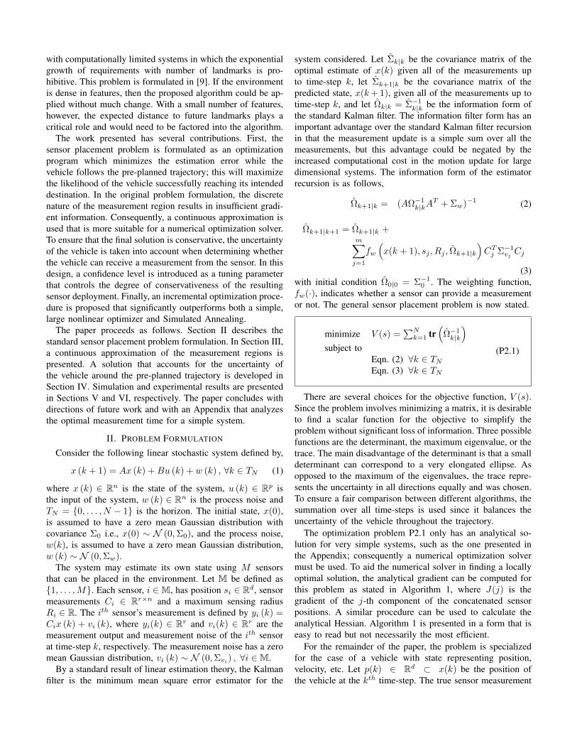
where d = ‖p− s‖ is the distance between the sensor and thevehicle. The function is a transformed sigmoid decay functionwith two parameters that control the shape. The parameter αaffects how quickly the function decays to zero beyond themaximum sensing radius R and is calculated through definingthe value of the function at the maximum sensing radius. Theparameter β controls the width of the shoulder. As β increases,the weighting function approaches the true sensing region.Figure 1 illustrates the weighting function for a maximumsensing radius of R = 2 meters, for an α parameter defined

by gw(2) = 0.01, and for values of β = [5, 10, 15, 20, 25, 30].The weighting function is approximately 0 when the vehicle isoutside the maximum sensing region and less than 1 when thevehicle is inside the sensing region. Therefore, this form ofthe weighting function is a conservative approximation of thetrue sensor weighting function which is a necessary conditionto obtain a realistic solution. Since the function is continuousand smooth everywhere, it has a well defined derivative whichis a major benefit for the numerical optimization solver.

0 0.5 1 1.5 2 2.5 30

0.25

0.5

0.75

1

distance

wei

ght

β = 5β = 10β = 15β = 20β = 25β = 30

Fig. 1. The weighting function, gw(d), for various values of the parameter βwith a maximum sensing radius of 2 meters and α is defined as gw(2) = 0.01.As β increases, the weighting function approaches the true weighting function.

IV. ACCOUNTING FOR UNCERTAINTY

For certain systems with large process noise, the pre-planned trajectory is not a good estimate of the vehicle’s pathif the system is not provided with enough measurements toaccurately estimate its state. Consequently, Eqn. (5) cannotbe used in its current form. Rather, the uncertainty in thevehicle’s position, p, at each time-step will need to be takeninto account. For the system considered, the estimate of theposition of the vehicle at each time-step has a Gaussian dis-tribution. Unfortunately the Gaussian distribution has infinitesupport, but luckily most of the probability distribution iscentered closely around the mean. Therefore, only a regionin the neighborhood of the pre-planned positions will haveto be considered for conservatively estimating whether thevehicle will receive a measurement from a sensor. This regionis represented by the ellipsoid Eρ. Consequently, d in Eqn. (5)can be replaced with Θ(p, s, Eρ) = max

o∈Eρ‖o − s‖, which is

defined as the maximum distance from the sensor position, s,to any point contained within the ellipsoid, Eρ.

For a multivariate Gaussian random variable there is anatural choice for the ellipsoid that represents the uncertaintyin the vehicle’s position. Consider the d-D position of thevehicle, p ∼ N (µ,Σ), where p ∈ Rd. A confidence level,δ, can be specified that results in a corresponding confidenceellipsoid, Eρ, such that, p (p ∈ Eρ) = δ. Given this definition,there are an infinite number of choices for the ellipsoid, but itwill be restricted to be centered around the mean µ.

Define the random variable, z ∈ R such thatz = (p− µ)TΣ−1(p− µ), which is a measure of the distanceof p from µ. It is well known that z has a Chi-square distribu-tion, X 2

d . The confidence ellipsoid, parameterized by ρ, is thendefined as, Eρ =

p ∈ Rd|z ≤ ρ

. Once the confidence level,

δ, is specified, the confidence ellipsoid parameter is calculatedvia ρ = F−1X 2

d(δ) where FX 2

dis the chi-square cumulative

distribution function. In this formulation, the confidence levelis a tuning parameter that controls the conservativeness of thesolution.

A. Example Objective Function

Several important properties of the objective function cannow be demonstrated through a simple example. Consider thedouble integrator system with 1D position defined by,

A=

[1 ∆t0 1

], B=

[0.5∆t2

∆t

], Σw=1× 10−4I,

Ci=[

1 0], Σvi =0.5, Ri=0.5,∀i∈1, 2

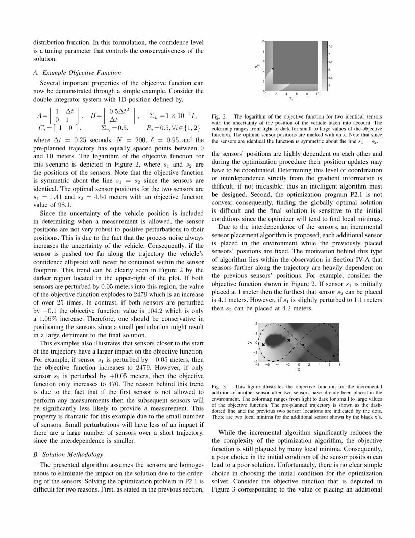
where ∆t = 0.25 seconds, N = 200, δ = 0.95 and thepre-planned trajectory has equally spaced points between 0and 10 meters. The logarithm of the objective function forthis scenario is depicted in Figure 2, where s1 and s2 arethe positions of the sensors. Note that the objective functionis symmetric about the line s1 = s2 since the sensors areidentical. The optimal sensor positions for the two sensors ares1 = 1.41 and s2 = 4.54 meters with an objective functionvalue of 98.1.

Since the uncertainty of the vehicle position is includedin determining when a measurement is allowed, the sensorpositions are not very robust to positive perturbations to theirpositions. This is due to the fact that the process noise alwaysincreases the uncertainty of the vehicle. Consequently, if thesensor is pushed too far along the trajectory the vehicle’sconfidence ellipsoid will never be contained within the sensorfootprint. This trend can be clearly seen in Figure 2 by thedarker region located in the upper-right of the plot. If bothsensors are perturbed by 0.05 meters into this region, the valueof the objective function explodes to 2479 which is an increaseof over 25 times. In contrast, if both sensors are perturbedby −0.1 the objective function value is 104.2 which is onlya 1.06% increase. Therefore, one should be conservative inpositioning the sensors since a small perturbation might resultin a large detriment to the final solution.

This examples also illustrates that sensors closer to the startof the trajectory have a larger impact on the objective function.For example, if sensor s1 is perturbed by +0.05 meters, thenthe objective function increases to 2479. However, if onlysensor s2 is perturbed by +0.05 meters, then the objectivefunction only increases to 470. The reason behind this trendis due to the fact that if the first sensor is not allowed toperform any measurements then the subsequent sensors willbe significantly less likely to provide a measurement. Thisproperty is dramatic for this example due to the small numberof sensors. Small perturbations will have less of an impact ifthere are a large number of sensors over a short trajectory,since the interdependence is smaller.

B. Solution Methodology

The presented algorithm assumes the sensors are homoge-neous to eliminate the impact on the solution due to the order-ing of the sensors. Solving the optimization problem in P2.1 isdifficult for two reasons. First, as stated in the previous section,

0 2 4 6 8 100

2

4

6

8

10

s1

s 2

5

5.5

6

6.5

7

7.5

Fig. 2. The logarithm of the objective function for two identical sensorswith the uncertainty of the position of the vehicle taken into account. Thecolormap ranges from light to dark for small to large values of the objectivefunction. The optimal sensor positions are marked with an x. Note that sincethe sensors are identical the function is symmetric about the line s1 = s2.

the sensors’ positions are highly dependent on each other andduring the optimization procedure their position updates mayhave to be coordinated. Determining this level of coordinationor interdependence strictly from the gradient information isdifficult, if not infeasible, thus an intelligent algorithm mustbe designed. Second, the optimization program P2.1 is notconvex; consequently, finding the globally optimal solutionis difficult and the final solution is sensitive to the initialconditions since the optimizer will tend to find local minimas.

Due to the interdependence of the sensors, an incrementalsensor placement algorithm is proposed; each additional sensoris placed in the environment while the previously placedsensors’ positions are fixed. The motivation behind this typeof algorithm lies within the observation in Section IV-A thatsensors further along the trajectory are heavily dependent onthe previous sensors’ positions. For example, consider theobjective function shown in Figure 2. If sensor s1 is initiallyplaced at 1 meter then the furthest that sensor s2 can be placedis 4.1 meters. However, if s1 is slightly perturbed to 1.1 metersthen s2 can be placed at 4.2 meters.

−8 −6 −4 −2 0 2 4 6 8−2

−1

0

1

2

x

y

Fig. 3. This figure illustrates the objective function for the incrementaladdition of another sensor after two sensors have already been placed in theenvironment. The colormap ranges from light to dark for small to large valuesof the objective function. The pre-planned trajectory is shown as the dash-dotted line and the previous two sensor locations are indicated by the dots.There are two local minima for the additional sensor shown by the black x’s.

While the incremental algorithm significantly reduces thethe complexity of the optimization algorithm, the objectivefunction is still plagued by many local minima. Consequently,a poor choice in the initial condition of the sensor position canlead to a poor solution. Unfortunately, there is no clear simplechoice in choosing the initial condition for the optimizationsolver. Consider the objective function that is depicted inFigure 3 corresponding to the value of placing an additional

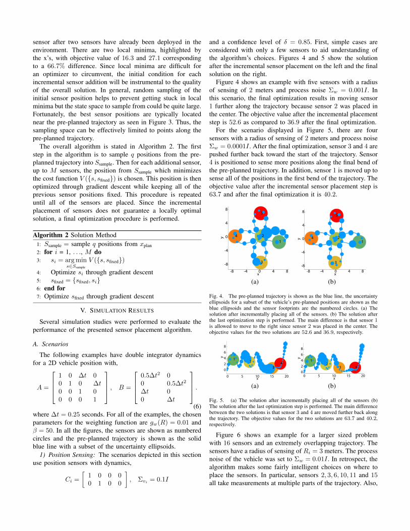
sensor after two sensors have already been deployed in theenvironment. There are two local minima, highlighted bythe x’s, with objective value of 16.3 and 27.1 correspondingto a 66.7% difference. Since local minima are difficult foran optimizer to circumvent, the initial condition for eachincremental sensor addition will be instrumental to the qualityof the overall solution. In general, random sampling of theinitial sensor position helps to prevent getting stuck in localminima but the state space to sample from could be quite large.Fortunately, the best sensor positions are typically locatednear the pre-planned trajectory as seen in Figure 3. Thus, thesampling space can be effectively limited to points along thepre-planned trajectory.

The overall algorithm is stated in Algorithm 2. The firststep in the algorithm is to sample q positions from the pre-planned trajectory into Ssample. Then for each additional sensor,up to M sensors, the position from Ssample which minimizesthe cost function V (s, sfixed) is chosen. This position is thenoptimized through gradient descent while keeping all of theprevious sensor positions fixed. This procedure is repeateduntil all of the sensors are placed. Since the incrementalplacement of sensors does not guarantee a locally optimalsolution, a final optimization procedure is performed.

Algorithm 2 Solution Method1: Ssample = sample q positions from xplan2: for i = 1, . . ., M do3: si = arg min

s∈Ssample

V (s, sfixed)

4: Optimize si through gradient descent5: sfixed = sfixed, si6: end for7: Optimize sfixed through gradient descent

V. SIMULATION RESULTS

Several simulation studies were performed to evaluate theperformance of the presented sensor placement algorithm.

A. Scenarios

The following examples have double integrator dynamicsfor a 2D vehicle position with,

A =

1 0 ∆t 00 1 0 ∆t0 0 1 00 0 0 1

, B =

0.5∆t2 00 0.5∆t2

∆t 00 ∆t

.(6)

where ∆t = 0.25 seconds. For all of the examples, the chosenparameters for the weighting function are gw(R) = 0.01 andβ = 50. In all the figures, the sensors are shown as numberedcircles and the pre-planned trajectory is shown as the solidblue line with a subset of the uncertainty ellipsoids.

1) Position Sensing: The scenarios depicted in this sectionuse position sensors with dynamics,

Ci =

[1 0 0 00 1 0 0

], Σvi = 0.1I

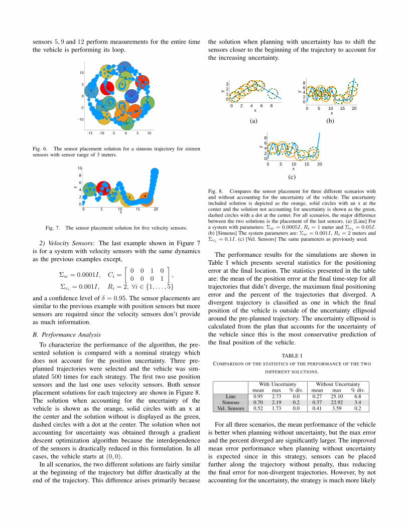
and a confidence level of δ = 0.85. First, simple cases areconsidered with only a few sensors to aid understanding ofthe algorithm’s choices. Figures 4 and 5 show the solutionafter the incremental sensor placement on the left and the finalsolution on the right.

Figure 4 shows an example with five sensors with a radiusof sensing of 2 meters and process noise Σw = 0.001I . Inthis scenario, the final optimization results in moving sensor1 further along the trajectory because sensor 2 was placed inthe center. The objective value after the incremental placementstep is 52.6 as compared to 36.9 after the final optimization.

For the scenario displayed in Figure 5, there are foursensors with a radius of sensing of 2 meters and process noiseΣw = 0.0001I . After the final optimization, sensor 3 and 4 arepushed further back toward the start of the trajectory. Sensor4 is positioned to sense more positions along the final bend ofthe pre-planned trajectory. In addition, sensor 1 is moved up tosense all of the positions in the first bend of the trajectory. Theobjective value after the incremental sensor placement step is63.7 and after the final optimization it is 40.2.

-8 -4 0 4 8

-8

-4

0

4

8

12

3

4

5

x

y

-8 -4 0 4 8-8

-4

0

4

8

12

3

4

5

x

y

(a) (b)

Fig. 4. The pre-planned trajectory is shown as the blue line, the uncertaintyellipsoids for a subset of the vehicle’s pre-planned positions are shown as theblue ellipsoids and the sensor footprints are the numbered circles. (a) Thesolution after incrementally placing all of the sensors. (b) The solution afterthe last optimization step is performed. The main difference is that sensor 1is allowed to move to the right since sensor 2 was placed in the center. Theobjective values for the two solutions are 52.6 and 36.9, respectively.

0 5 10 15 20

0

2

4

6

8

12

34

x

y

0 5 10 15 200

2

4

6

8

12

3 4

x

y

(a) (b)

Fig. 5. (a) The solution after incrementally placing all of the sensors (b)The solution after the last optimization step is performed. The main differencebetween the two solutions is that sensor 3 and 4 are moved further back alongthe trajectory. The objective values for the two solutions are 63.7 and 40.2,respectively.

Figure 6 shows an example for a larger sized problemwith 16 sensors and an extremely overlapping trajectory. Thesensors have a radius of sensing of Ri = 3 meters. The processnoise of the vehicle was set to Σw = 0.01I . In retrospect, thealgorithm makes some fairly intelligent choices on where toplace the sensors. In particular, sensors 2, 3, 6, 10, 11 and 15all take measurements at multiple parts of the trajectory. Also,

sensors 5, 9 and 12 perform measurements for the entire timethe vehicle is performing its loop.

-15 -10 -5 0 5 10

-10

-5

0

5

10

1

2

3

45

6

7

8

9

10

1113

14

15

16

12

Fig. 6. The sensor placement solution for a sinuous trajectory for sixteensensors with sensor range of 3 meters.

0 5 10 15 200

2

4

6

8

10

12

3 45

x

y

Fig. 7. The sensor placement solution for five velocity sensors.

2) Velocity Sensors: The last example shown in Figure 7is for a system with velocity sensors with the same dynamicsas the previous examples except,

Σw = 0.0001I, Ci =

[0 0 1 00 0 0 1

],

Σvi = 0.001I, Ri = 2, ∀i ∈ 1, . . . , 5

and a confidence level of δ = 0.95. The sensor placements aresimilar to the previous example with position sensors but moresensors are required since the velocity sensors don’t provideas much information.

B. Performance Analysis

To characterize the performance of the algorithm, the pre-sented solution is compared with a nominal strategy whichdoes not account for the position uncertainty. Three pre-planned trajectories were selected and the vehicle was sim-ulated 500 times for each strategy. The first two use positionsensors and the last one uses velocity sensors. Both sensorplacement solutions for each trajectory are shown in Figure 8.The solution when accounting for the uncertainty of thevehicle is shown as the orange, solid circles with an x atthe center and the solution without is displayed as the green,dashed circles with a dot at the center. The solution when notaccounting for uncertainty was obtained through a gradientdescent optimization algorithm because the interdependenceof the sensors is drastically reduced in this formulation. In allcases, the vehicle starts at (0, 0).

In all scenarios, the two different solutions are fairly similarat the beginning of the trajectory but differ drastically at theend of the trajectory. This difference arises primarily because

the solution when planning with uncertainty has to shift thesensors closer to the beginning of the trajectory to account forthe increasing uncertainty.

0 2 4 6 8

0123

x

y

0 5 10 15 20

02468

x

y

(a) (b)

0 5 10 15 2002468

x

y

(c)

Fig. 8. Compares the sensor placement for three different scenarios withand without accounting for the uncertainty of the vehicle. The uncertaintyincluded solution is depicted as the orange, solid circles with an x at thecenter and the solution not accounting for uncertainty is shown as the green,dashed circles with a dot at the center. For all scenarios, the major differencebetween the two solutions is the placement of the last sensors. (a) [Line] Fora system with parameters: Σw = 0.0005I , Ri = 1 meter and Σvi = 0.05I .(b) [Sinuous] The system parameters are: Σw = 0.001I , Ri = 2 meters andΣvi = 0.1I . (c) [Vel. Sensors] The same parameters as previously used.

The performance results for the simulations are shown inTable I which presents several statistics for the positioningerror at the final location. The statistics presented in the tableare: the mean of the position error at the final time-step for alltrajectories that didn’t diverge, the maximum final positioningerror and the percent of the trajectories that diverged. Adivergent trajectory is classified as one in which the finalposition of the vehicle is outside of the uncertainty ellipsoidaround the pre-planned trajectory. The uncertainty ellipsoid iscalculated from the plan that accounts for the uncertainty ofthe vehicle since this is the most conservative prediction ofthe final position of the vehicle.

TABLE ICOMPARISON OF THE STATISTICS OF THE PERFORMANCE OF THE TWO

DIFFERENT SOLUTIONS.

With Uncertainty Without Uncertaintymean max % div. mean max % div.

Line 0.95 2.73 0.0 0.27 25.10 6.8Sinuous 0.70 2.19 0.2 0.37 22.92 3.4

Vel. Sensors 0.52 1.73 0.0 0.41 3.59 0.2

For all three scenarios, the mean performance of the vehicleis better when planning without uncertainty, but the max errorand the percent diverged are significantly larger. The improvedmean error performance when planning without uncertaintyis expected since in this strategy, sensors can be placedfurther along the trajectory without penalty, thus reducingthe final error for non-divergent trajectories. However, by notaccounting for the uncertainty, the strategy is much more likely

to result in divergent trajectories. It is also interesting to notethat for the velocity sensors scenario, the performance statisticsare very similar for both planning strategies. This is due to thefact that velocity sensors accumulate a large amount of drift inthe position estimate of the vehicle. Thus, there is less benefitin incorporating the uncertainty in the planning stage.

C. Comparison to Simulated Annealing

For comparison, the proposed algorithm was evaluatedagainst Simulated Annealing (SA). Since SA is a stochasticalgorithm it has the potential to avoid local minima and ap-proach the globally optimal solution. The proposed algorithmand SA were evaluated on three different scenarios. Figure 9shows a histogram of the relative difference, VSA−V

V , for 50trials of each scenario.

In the first scenario, the pre-planned trajectory is a simple45 line and there are 3 sensors with a sensing radius of 6 me-ters. Figure 9(a) shows a histogram of the relative performancebetween the proposed algorithm and SA. Even for this simplescenario, SA has difficultly consistently finding a reasonablesolution. In 28% of the trials SA had an objective value largerthan 50 times the proposed solution. In the next scenario, SAwas run for the example shown in Figure 4 and the histogramof the relative performance is shown in Figure 9(b). For thefinal scenario, both algorithms were evaluated on the sinuoustrajectory displayed in Figure 5 and the results are shownin Figure 9(c). In this example, SA was able to find a 20%better solution than the proposed algorithm 30% of the time,but 70% of the solutions were over 6 times worse than theproposed algorithm. Consequently, even though SA sometimescan find a better solution, the proposed algorithm consistentlyfinds reasonable solutions. In addition, SA ran slower than theproposed algorithm by a factor of 22, 16 and 13.

0 100 300 500 7000

10

20

30

40

Relative Difference

His

togr

am

0 2 4 6 8 10 12 140

10

20

3035

Relative Difference

His

togr

am

−1 0 1 2 3 4 5 60

10

20

3035

Relative Difference

His

togr

am

(a) (b) (c)

Fig. 9. Comparison of the relative performance between the proposedalgorithm and Simulated Annealing for three different examples. A positivenumber means that Simulated Annealing found a worse solution than theproposed algorithm.

VI. EXPERIMENTAL RESULTS

The sensor placement strategies were also evaluated ona quadrotor unmanned aerial vehicle. The vehicle has anonboard inertial measurement unit which provides three-axisattitude, attitude rate and acceleration measurements. An ex-ternal Vicon [10] positioning system is also used to providemeasurements of the vehicle’s position with respect to a globalcoordinate frame.

With any aerial vehicle, the state (position, orientation andvelocity) estimation is critical to a successful flight since smallerrors can easily lead to a disastrous crash. With this in mind,instead of withholding Vicon measurements when the vehicle

is outside of the sensing regions, the vehicle was provided withdegraded measurements to prevent any major catastrophes.

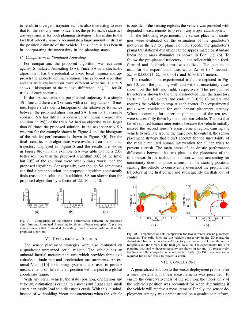
In the following experiments, the sensor placement strate-gies were evaluated on the estimation of the quadrotor’smotion in the 2D x-y plane. For low speeds, the quadrotor’splanar translational dynamics can be approximated by standardlinear point mass dynamics as shown in Eqn. (1), (6). Tofollow the pre-planned trajectory, a controller with both feed-forward and feedback terms was utilized. The parametersused for the experimental tests were: ∆t = 0.05 seconds,Σw = 0.00001I , Σvi = 0.001I and Ri = 0.25 meters.

The results of the experimental trials are depicted in Fig-ure 10, with the planning with and without uncertainty casesshown on the left and right, respectively. The pre-plannedtrajectory is shown by the blue, dash-dotted line; the trajectorystarts at (−1, 0) meters and ends at (−0.25, 0) meters andrequires the vehicle to stop at each corner. Ten experimentaltrials were conducted for each sensor placement strategy.When accounting for uncertainty, nine out of the ten testswere successfully flown by the quadrotor vehicle. The test thatfailed required human intervention because the vehicle initiallymissed the second sensor’s measurement region, causing thevehicle to oscillate around the trajectory. In contrast, the sensorplacement strategy that didn’t account for the uncertainty ofthe vehicle required human intervention for all ten trials toprevent a crash. The main cause of the drastic performancedifferences between the two plans is the placement of thefirst sensor. In particular, the solution without accounting foruncertainty does not place a sensor at the starting position,causing the vehicle to consistently overshoot the pre-plannedtrajectory at the first corner and subsequently oscillate out ofcontrol.

-1 -0.5 0 0.5 1

0

0.5

1

1.5

x (meters)

y (m

eter

s)

-1 -0.5 0 0.5 1

-0.5

0

0.5

1

1.5

x (meters)

y (m

eter

s)

(a) (b)

Fig. 10. Experimental data comparison for two different sensor placementstrategies. The solid lines are the vehicle’s trajectory in the 2D plane, thedash-dotted line is the pre-planned trajectory, the colored circles are the sensorfootprints and the x mark is the final goal location. The experimental trials forplanning with and without uncertainty are shown in (a) and (b), respectively.(a) Successfully completes nine out of ten trials. (b) Pilot intervention isrequired for all ten trials to prevent a crash.

VII. CONCLUSIONS

A generalized solution to the sensor deployment problem fora linear system with linear measurements was presented. Toensure the conservativeness of the solution, the uncertainty ofthe vehicle’s position was accounted for when determining ifthe vehicle will receive a measurement. Finally, the sensor de-ployment strategy was demonstrated on a quadrotor platform,

where the proposed algorithm showed significant performanceincreases over other strategies.

There are several interesting areas of future work thatthe authors wish to explore. First, the case of non-radialsensing regions due to obstacle occlusions should be exploredwhich will increase the applicability of the algorithm. Anotherextension to the algorithm is to incorporate nonlinear systemdynamics as well as nonlinear sensor measurements. Lastly,the authors wish to extend the algorithm to handle heteroge-neous sensors; this presents a challenging addition since theordering of the sensors heavily impacts the final solution.

ACKNOWLEDGMENT

The authors wish to thank Deborah Meduna for numerousdiscussions during the preparation of the paper.

APPENDIXANALYTICAL SOLUTION

For simple systems, an analytical solution to the optimiza-tion problem in P2.1 can be found. Consider a 1D system thathas dynamics,

xk+1 = xk + ∆tuk + wk. (7)

where xk ∈ R, wk ∼ N (0, σw) and k ∈ 1, . . . , N .In the current scenario, the system can only take a singlemeasurement, ys = xs + v with v ∼ N (0, σv), attime-step, s. The optimal measurement time can be solved forby differentiating the objective function and setting it equal to0 which results in:

s∗ =

− σ0σw

,1

σw

(−3

4(σ0 + σv) +

1

4(N + 1)σw±

1

4

√(σ0 + 9σv + (N + 1)σw) (σ0 + σv + (N + 1)σw)

).

(8)It is important to note that there is no guarantee that the valuefor s∗ will be an integer. An integer solution, s∗, can bedetermined by rounding s∗. The performance of this roundedsolution is upper bounded away from the optimal solution byV (s∗)−V (s∗). Also, the optimal solution is not guaranteed toreturn a solution in the range 1, . . . , N, but these cases canstill provide valuable insight into the optimal sensing time.

PERTURBATION ANALYSIS

An interesting analysis to perform on the optimal sensingtime is how the solution varies due to perturbations in thesystem parameters.

Time Horizon N :

One parameter of interest is the time horizon. The derivativeof the optimal sensing time with respect to the time horizonis,

∂s∗

∂N=

1 + 5σv + σ0 + (N + 1)σw

4√

(9σv + σ0 + (N + 1)σw)(σv + σ0 + (N + 1)σw).

(9)The steady state change as N approaches ∞ islimN→∞

∂s∗

∂N = 12 . Consequently, as N increases the

optimal sensing time’s dependence on the parameters of thesystem decreases; therefore, if the time horizon is increasedby one time-step, the optimal sensing time will only changeby 0.5.

Process Noise σw:

Characteristics of the optimal sensor measurement time withrespect to changes in the process noise can also be determinedanalytically. Some of the important results from this analysisare as follows. As the process noise, σw, approaches 0 islimσw→0+ s

∗ = −∞, which is ill-formed because the sensingtime is restricted to s ∈ 1, . . . , N, but a trend can still beextracted from the result. As the process noise decreases, theoptimal sensing time also decreases toward the first possiblemeasurement time. As σw approaches ∞ is limσw→∞ s∗ =12 (N + 1). Consequently, as the process noise grows towardinfinity the optimal sensing time isn’t dependent on any ofthe system parameters and approaches the middle of the timehorizon.

Measurement Noise σv:

The properties of the optimal sensing time can also beanalyzed with respect to the measurement noise. As themeasurement noise, σv , tends to 0,

limσv→0+

s∗ =(N + 1)σw − 2σ0

2σw≤ 1

2(N + 1) (10)

which is bounded to the first half of the time horizon. As σvapproaches ∞,

limσv→∞

s∗ =2(N + 1)σw − σ0

3σw≤ 2

3(N + 1) (11)

which is dependent on the other system parameters but can bebounded to the first two-thirds of the time horizon.

REFERENCES

[1] P. Misra and P. Enge, Global Positioning System: Signals, Measurements,and Performance. Lincoln, MA, USA: Ganga-Jamuna Press, second ed.,2006.

[2] M. Phatak, “Recursive method for optimum GPS satellite selection,”Aerospace and Electronic Systems, IEEE Transactions on, vol. 37,pp. 751–754, April 2001.

[3] M. Kihara and T. Okada, “A satellite selection method and accuracy forthe global positioning system,” Navigation, vol. 31, no. 1, 1984.

[4] D. B. Jourdan and N. Roy, “Optimal sensor placement for agentlocalization,” in Proceedings of the IEEE/ION Position Location andNavigation Symposium (PLANS 2006), (San Diego, CA), April 2006.

[5] H. Zhang, “Two-dimensional optimal sensor placement,” IEEE Trans-actions on Systems, Man, and Cybernetics, vol. 25, May 1995.

[6] S. Ponda and E. Frazzoli, “Trajectory optimization for target localizationusing small unmanned aerial vehicles,” in AIAA Conf. on Guidance,Navigation, and Control, (Chicago, IL), 2009.

[7] A. Sinha, T. Kirubarajan, and Y. Bar-Shalom, “Optimal cooperativeplacement of GMTI UAVs for ground target tracking,” in Proceedingsof the IEEE Aerospace Conference, (Big Sky, MT), March 2004.

[8] S. Martinez and F. Bullo, “Optimal sensor placement and motioncoordination for target tracking,” Automatica, vol. 42, pp. 661–668, April2006.

[9] H. Strasdat, C. Stachniss, and W. Burgard, “Which landmark is useful?Learning selection policies for navigation in unknown environments,”in Proceedings of the IEEE International Conference on RoboticsAutomation (ICRA), 2009.

[10] Vicon, Vicon MX Systems. visited January 2010.http://www.vicon.com/products/viconmx.html.