Embed Size (px)
Citation preview

SENSOR-BASED AUTOMATION OF IRRIGATION OF BERMUDAGRASS
By
BERNARD CARDENAS-LAILHACAR
A THESIS PRESENTED TO THE GRADUATE SCHOOL OF THE UNIVERSITY OF FLORIDA IN PARTIAL FULFILLMENT
OF THE REQUIREMENTS FOR THE DEGREE OF MASTER OF SCIENCE
UNIVERSITY OF FLORIDA
2006

Copyright 2006
by
Bernard Cardenas-Lailhacar

To my parents and sons

iv
ACKNOWLEDGMENTS
In the first place, I wish to thank my parents for their always enormous and
unconditional love, support, and guidance; my sons for being the most adorable human
beings I have ever met; my ex-wife for taking care of them while I was completing my
studies, her understanding, patience, and sacrifice; and my amorcita for her enormous
support, understanding, patience and, most of all, her immense love. Next, I would like to
thank all my thesis committee members for being not just professors, but great human
beings: Dr. Dorota Z. Haman and Dr. Grady L. Miller, also for their guidance and
patience, and a huge thank you goes to Dr. Michael D. Dukes, for giving me the
opportunity to work with him, which was always a lot of work, but also a pleasure. Also,
I wish to give a special thank you to Melissa B. Haley for being always ready to help me.
Lastly, I would also like to thank Engineer Larry Miller, Senior Engineering Technician
Danny Burch, and students Mary Shedd, Stephen Hanks, Clay Coarsey, Brent Addison,
Jason Frank, and Clay Breazeale for their assistance on this research. This research was
supported by the Pinellas-Anclotte Basin Board of the Southwest Water Management
District, the Florida Nursery and Landscape Growers Association, and the Florida
Agricultural Experiment Station.
v
TABLE OF CONTENTS page
ACKNOWLEDGMENTS ................................................................................................. iv
LIST OF TABLES........................................................................................................... viii
LIST OF FIGURES .............................................................................................................x
ABSTRACT.......................................................................................................................xv
CHAPTER
1 INTRODUCTION ........................................................................................................1
Water.............................................................................................................................1 Water Demand ..............................................................................................................2 Water Use .....................................................................................................................2 Water Use Restrictions .................................................................................................3 Landscapes in Florida ...................................................................................................5 Irrigation .......................................................................................................................6
Irrigation Timers....................................................................................................6 Soil Moisture Content Measurement.....................................................................8
Granular matrix sensor ...................................................................................8 Modern soil moisture sensors.........................................................................9
Controllers ...........................................................................................................11 Automatic Control of Irrigation...........................................................................12 Rain Sensors ........................................................................................................13
Irrigation and Turfgrass Quality .................................................................................15
2 SENSOR-BASED AUTOMATION OF IRRIGATION OF BERMUDAGRASS....20
Introduction.................................................................................................................20 Materials and Methods ...............................................................................................25
Treatments ...........................................................................................................27 Uniformity Test ...................................................................................................28 Dry-Wet Analysis................................................................................................29 Plot Irrigation Management and Data Collection................................................30 Data Analysis.......................................................................................................33
Results and Discussion ...............................................................................................34 Uniformity Tests..................................................................................................34
vi
Dry-Wet Analysis................................................................................................34 Rainfall ................................................................................................................35 Irrigation Events ..................................................................................................36 Irrigation Application Comparisons ....................................................................42
Time-based treatments vs. SMS-based treatments.......................................42 Time-based treatments .................................................................................42 Comparisons between SMS-irrigation frequencies......................................44 Soil moisture sensor-brands comparison......................................................45 Brand comparisons within irrigation frequencies ........................................46 Overall comparison ......................................................................................47
Automation of Irrigation Systems .......................................................................49 Turfgrass Quality.................................................................................................50
Summary and Conclusions .........................................................................................51
3 EXPANDING DISK RAIN SENSOR PERFORMANCE AND POTENTIAL IRRIGATION WATER SAVINGS ...........................................................................93
Rain Sensors ...............................................................................................................93 Advantages ..........................................................................................................94 Types and Methods..............................................................................................94 Installation ...........................................................................................................96 Objectives ............................................................................................................96
Materials and Methods ...............................................................................................97 Data......................................................................................................................97 Treatments ...........................................................................................................98 Statistical Analysis ..............................................................................................99
Results and Discussion ...............................................................................................99 Climatic Conditions.............................................................................................99 Number of Times in Bypass Mode......................................................................99 Depth of Rainfall Before Shut Off ....................................................................100 Duration in Irrigation Bypass Mode (Dry-Out Period) .....................................102 Potential Water Savings ....................................................................................103 Payback Period ..................................................................................................104
Summary and Conclusions .......................................................................................105
4 GRANULAR MATRIX SENSOR PERFORMANCE COMPARED TO TENSIOMETER IN A SANDY SOIL.....................................................................119
Tensiometers.............................................................................................................119 Granular Matrix Sensors...........................................................................................121 GMS – Tensiometer Comparison .............................................................................122 Objectives .................................................................................................................122 Materials and Methods .............................................................................................122
Experimental Set-Up .........................................................................................123 ECH2O Probes Calibration ................................................................................123 Treatments .........................................................................................................124 Data....................................................................................................................124

vii
Results and Discussion .............................................................................................125 Calibration of the ECH2O Probe .......................................................................125 GMSs versus Tensiometers. ..............................................................................125
Conclusions...............................................................................................................126
5 CONCLUSIONS AND FUTURE WORK...............................................................140
Conclusions...............................................................................................................140 Future Work..............................................................................................................142
APPENDIX
A LIST OF ABBREVIATIONS...................................................................................144
B STATISTICAL ANALYSES ...................................................................................145
LIST OF REFERENCES.................................................................................................199
BIOGRAPHICAL SKETCH ...........................................................................................208

viii
LIST OF TABLES
Table page 2-1. Irrigation treatment codes and descriptions...............................................................54
2-2. Monthly irrigation depth to replace historical evapotranspiration, assuming system efficiency of 60%, and considering effective rainfall. .................................54
2-3. Total number and percent of overridden scheduled irrigation cycles; 2004 and 2005. .........................................................................................................................55
2-4. Percent of irrigation cycles allowed by the SMS-based treatments through the experimental months of 2004 and 2005. ..................................................................56
2-5. Cumulative irrigation depth applied to treatments, statistical comparisons between them, and percent of water savings compared to 2-WRS, 2-DWRS, and 2-WORS; year 2004. ................................................................................................57
2-6. Cumulative irrigation depth applied to treatments, statistical comparisons between them, and percent of water savings compared to 2-WRS, 2-DWRS, and 2-WORS; year 2005. ................................................................................................58
2-7. Total cumulative irrigation depth applied to treatments, statistical comparisons between them, and percent of water savings compared to 2-WRS, 2-DWRS, and 2-WORS; years 2004 + 2005. ..................................................................................59
3-1. Treatments description. ...........................................................................................107
3-2. Average depth of rainfall before rain sensors switched to bypass mode.................107
3-3. Large rainfall events not bypassed by treatment 3-MC...........................................107
3-4. Large rainfall events not bypassed by treatment 13-MC.........................................108
3-5. Large rainfall events not bypassed by treatment 25-MC.........................................108
3-6. Hours after rain stopped and sensors switched to bypass mode; treatment 3-MC. .108
3-7. Hours after rain stopped and sensors switched to bypass mode; treatment 13-MC.109

ix
3-8. WL replications that switched to bypass mode in absence of rainfall, elapsed time that they remained in bypass mode, and relative humidity at the time when this occurred. .................................................................................................................109
3-9. Total potential water savings per treatment.............................................................109
3-10. Potential payback period per treatment. ................................................................110
4-1. Treatments. ..............................................................................................................128
4-2. GMS-Tensiometer crossing points. .........................................................................128

x
LIST OF FIGURES
Figure page 1-1. Components of an automated irrigation system: A) timer, B) power supply, C)
soil moisture sensor-controller circuitry, D) soil moisture sensor, and E) solenoid valve...........................................................................................................16
1-2. Granular matrix sensors (GMS) ................................................................................17
1-3. Components of an automated irrigation system. 1) Timer, and 2) soil moisture sensor-controllers from different brands. .................................................................18
1-4. Rain shut-off switch...................................................................................................19
1-5. The expanding material of a rain shut-off switch......................................................19
2-1. Soil water retention curve from tensiometers and calibrated ECH2O probe readings. ...................................................................................................................60
2-2. Soil moisture sensor brands tested in this study. .......................................................61
2-3. Irrigation controls as installed for this study: soil moisture sensors-controllers brands: A) Rain Bird, B) Water Watcher, C) Acclima, and D) Irrometer, and irrigation timer E) Rain Bird. ...................................................................................62
2-4. Rain sensor installed for this study............................................................................63
2-5. Catch-can display for uniformity tests on turfgrass plots..........................................64
2-6. General view of the irrigation controls used in this study.........................................65
2-7. Pipes, flowmeters, valves, and wirings for this study. ..............................................65
2-8. Control board showing timers, soil moisture sensor-controllers, solenoid valves wiring, and flowmeters-datalogger (details are shown in the next s).......................66
2-9. Control board detail showing the solenoid valves control box. ................................67
2-10. Control board detail, flowmeter-datalogger boxes showing A) multiplexers, B) CR 10X datalogger used for this study. ...................................................................67
2-11. Automated weather station near turf plots for this study.........................................68
xi
2-12. ECH2O probe, capacitance soil moisture probe shown with a HOBO data logger as installed for this study. .........................................................................................69
2-13. Plot plan showing the low-quarter distribution uniformity testing results on each plot............................................................................................................................70
2-14. Plot plan showing average volumetric water content (%) on each plot during a relatively “dry” period. Plots in red were discarded, and plots in green were used for placement of SMSs. ............................................................................................71
2-15. Plot plan showing average volumetric water content (%) on each plot during a relatively “wet” condition. Plots in red were discarded, and plots in green were used for placement of SMSs.....................................................................................72
2-16. Plot plan with the modified completely randomized design (same color depicts treatment repetitions)................................................................................................73
2-17. Daily and cumulative rainfall in 2004. Note: rainfall for 5 Sep. (188 mm) and 6 Sep. (81 mm) is shown as a cumulative total (269 mm). .........................................74
2-18. Daily and cumulative rainfall in 2005. ....................................................................74
2-19. Cumulative number of irrigation events per treatment in 2004; A) time-based treatments, and soil moisture sensor-based treatments at irrigation frequencies of B) 1 d/w, C) 2 d/w, and D) 7 d/w. ............................................................................75
2-20 Cumulative number of irrigation events per treatment in 2005; A) time-based treatments, and soil moisture sensor-based treatments at irrigation frequencies of B) 1 d/w, C) 2 d/w, and D) 7 d/w. ............................................................................76
2-21. Maximum weekly irrigation water requirement (rainfall - ETo difference); year 2004. .........................................................................................................................77
2-22. Maximum weekly irrigation water requirement (rainfall - ETo difference); year 2005. .........................................................................................................................77
2-23. Volumetric moisture content through time, on treatment 0-NI, year 2004. ............78
2-24. Volumetric moisture content (VMC) through time, showing results of the scheduled irrigation cycles (SIC); treatment 1-AC, year 2004. ...............................79
2-25. Volumetric moisture content (VMC) through time, showing results of the scheduled irrigation cycles (SIC); treatment 1-IM, year 2004.................................80
2-26. Volumetric moisture content (VMC) through time, showing results of the scheduled irrigation cycles (SIC); treatment 1-RB, year 2004. ...............................81
xii
2-27. Volumetric moisture content (VMC) through time, showing results of the scheduled irrigation cycles (SIC); treatment 1-WW, year 2004. .............................82
2-28. Volumetric moisture content (VMC) through time, showing results of the scheduled irrigation cycles (SIC); treatment 2-AC, year 2004. ...............................83
2-29. Volumetric moisture content (VMC) through time, showing results of the scheduled irrigation cycles (SIC); treatment 2-IM, year 2004.................................84
2-30. Volumetric moisture content (VMC) through time, showing results of the scheduled irrigation cycles (SIC); treatment 2-RB, year 2004. ...............................85
2-31. Volumetric moisture content (VMC) through time, showing results of the scheduled irrigation cycles (SIC); treatment 2-WW, year 2004. .............................86
2-32. Volumetric moisture content (VMC) through time, showing results of the scheduled irrigation cycles (SIC); treatment 7-AC, year 2004. ...............................87
2-33. Volumetric moisture content (VMC) through time, showing results of the scheduled irrigation cycles (SIC); treatment 7-IM, year 2004.................................88
2-34. Volumetric moisture content (VMC) through time, showing results of the scheduled irrigation cycles (SIC); treatment 7-RB, year 2004. ...............................89
2-35. Volumetric moisture content (VMC) through time, showing results of the scheduled irrigation cycles (SIC); treatment 7-WW, year 2004. .............................90
2-36. Average irrigation depth applied by brand; years 2004 and 2005 (P<0.0001)........91
2-37. View of different plots where no evident turfgrass quality differences could be detected; A) good quality, B) dormant.....................................................................92
3-1. Mini-Click (Hunter Industries, Inc.) rain sensor. A) Rain threshold set slots, B) vent ring..................................................................................................................111
3-2. Wireless Rain-Click (Hunter Industries, Inc.) rain sensor. A) Ventilation window adjustment knob, B) ventilation windows, C) antenna. .........................................111
3-3. The expanding material of a rain shut-off switch....................................................112
3-4. Rain sensor experiment layout: A) Wireless Rain-Click rain sensors, B) Mini-Click rain sensors, C) Wireless Rain-Click receivers, D) multiplexers, E) CR 10X datalogger. ......................................................................................................112
3-5. Manual rain gauge measurements compared to tipping bucket rain gauge measurements. ........................................................................................................113
3-6. Daily and cumulative rainfall. .................................................................................113

xiii
3-7. Cumulative number of times rain sensors switched to bypass mode; average per treatment. Different letters indicate a significant difference by Duncan’s Multiple Range Test (P<0.05)................................................................................114
3-8. Cumulative number of times rain sensors switched to bypass mode; WL treatment, with replicates indicated by A-D...........................................................115
3-9. Cumulative number of times rain sensors switched to bypass mode; 3-MC treatment, with replicates indicated by A-D...........................................................115
3-10. Cumulative number of times rain sensors switched to bypass mode; 13-MC treatment, with replicates indicated by A-D...........................................................116
3-11. Cumulative number of times rain sensors switched to bypass mode; 25-MC treatment, with replicates indicated by A-D...........................................................116
3-12. Histogram and frequency distribution for 6-hour intervals in bypass mode; WL.117
3-13. Histogram and frequency distribution for 6-hour intervals in bypass mode; 3-MC..........................................................................................................................117
3-14. Histogram and frequency distribution for 6-hour intervals in bypass mode; 13-MC..........................................................................................................................118
4-1. MLT-RSU Tensiometer...........................................................................................129
4-2. Watermark GMS......................................................................................................129
4-3. Temperature sensor..................................................................................................130
4-4. ECH2O probe...........................................................................................................130
4-5. Experimental layout (top view). A) Tensiometers, B) Granular matrix sensors, C) ECH2O probe, and D) Thermometer......................................................................131
4-6. Watermark monitor..................................................................................................132
4-7. ECH2O probe hooked up to a HOBO Micro Station datalogger.............................132
4-8. Volumetric moisture content (VMC) from all three ECH2O probes compared to gravimetric measurements......................................................................................133
4-9. Soil water tension through time; treatment T0. .......................................................134
4-10. Soil water tension through time; treatment T5. .....................................................134
4-11. Soil water tension through time; treatment T15. ...................................................135
4-12. Soil water tension through time; treatment T50. ...................................................135
xiv
4-13. Soil water tension through time; detail showing when curves from GMS and tensiometers cross; treatment T0............................................................................136
4-14. Soil water tension through time; detail showing when curves from GMS and tensiometers cross; treatment T5............................................................................136
4-15. Soil water tension through time; detail showing when curves from GMS and tensiometers cross; treatment T15..........................................................................137
4-16. Soil water tension through time; detail showing when curves from GMS and tensiometers cross; treatment T50..........................................................................137
4-17. Relation between the average soil matric potential (SMP) from tensiometers and GMS. ......................................................................................................................138
4-18. Relation between the average soil matric potential (SMP) from tensiometers and GMS; excluding GMS data < 10 kPa.....................................................................139
xv
Abstract of Thesis Presented to the Graduate School
of the University of Florida in Partial Fulfillment of the Requirements for the Degree of Master of Science
SENSOR-BASED AUTOMATION OF IRRIGATION OF BERMUDAGRASS
By
Bernard Cardenas-Lailhacar
August 2006
Chair: Michael D. Dukes Major Department: Agricultural and Biological Engineering
Turfgrass in landscapes contributes to substantial cropped area in Florida. New
irrigation technologies could improve irrigation efficiency, promoting water conservation
and reducing the environmental impacts. The objectives of this research were to quantify
differences in irrigation water use and turf quality among 1) a soil moisture sensor-based
irrigation system compared to a time-based scheduling, 2) different commercial irrigation
soil moisture sensor (SMSs), 3) a time-based scheduling system with or without a rain
sensor (RS), and 4) the reliability of two commercially available expanding disk RS-
types. The experimental area consisted of common bermudagrass (Cynodon dactylon L.)
plots (3.66 x 3.66 m) in a completely randomized design, located in Gainesville, Florida.
The monitoring period for the irrigation treatments took place from 20 July through 14
December of 2004 and from 25 March through 31 August of 2005. Treatments consisted
of irrigating one, two, or seven days a week, each with four different commercial SMSs
brands. A non-irrigated control and time-based treatments were also implemented. In
xvi
addition, twelve Mini-Click (MC) and four Wireless Rain-Click (WL) rain sensor models
not connected to irrigation were monitored from 25 March through 31 December 2005.
For the MCs, three different thresholds were established: 3, 13, and 25 mm (codes 3-MC,
13-MC, and 25-MC, respectively). No significant differences in turfgrass quality among
irrigation treatments were detected. On average, SMS-based treatments reduced irrigation
water application compared to time-based treatments. The treatment without-rain-sensor
(2-WORS) used significantly (52%) more water than the with-rain-sensor treatment (2-
WRS). Most brands recorded significant irrigation water savings compared to 2-WRS,
which ranged from 54% to 88%, for the best performing sensors, and depending on the
irrigation frequency. Therefore SMS-systems represent a promising technology, because
of the water savings that they can accomplish, while maintaining an acceptable turfgrass
quality during rainy periods (944 and 732 mm of rainfall, for seasons 2004 and 2005,
respectively). On average, RS treatments WL, 3-MC, 13-MC, and 25-MC responded
close to their rainfall set points (1.4, 3.4, 10.0, and 24.5 mm, respectively). However,
some replications showed erratic behavior through time. The number of times that these
sensors shut off irrigation was inversely proportional to the magnitude of their set point
(81, 43, 30, and 8 times, respectively) with potential water savings following a similar
trend (363, 245, 142, and 25 mm, respectively). Under the relatively wet testing
conditions typical to Florida, the payback period could be less than a year, except for 25-
MC (around 7 years). Consequently, RSs are strongly recommended for use by
homeowners as a means to save water, but not when accuracy is required.

1
CHAPTER 1 INTRODUCTION
Turfgrass is the main cultivated crop in Florida with nearly four times the acreage
as the next largest crop, citrus (Hodges et al., 1994; United States Department of
Agriculture [USDA], 2005). Irrigation of residential, industrial, commercial, and
recreational turf areas is necessary to ensure acceptable turf quality. As a consequence of
problems related to drought, coupled with a steadily increasing demand for water
resources, the state of Florida has imposed restrictions on irrigation water use. Water
used for turfgrass irrigation, however, remains to be publicly discussed. The development
of Best Management Practices (BMPs) for irrigation water use in landscapes has become
an undeniable strategic, economic, and environmental issue for the state. New irrigation
technologies could improve irrigation efficiency, promoting water conservation and
reducing the environmental impacts of turfgrass culture, which is a major component of
landscapes in Florida.
Water
Florida receives an average of around 1400 mm of rainfall a year (National Oceanic
and Atmospheric Administration [NOAA], 2003). Unlike many areas dependent on
irrigation, annual rainfall in Florida typically exceeds evapotranspiration. Nevertheless,
irrigation is required because total annual rainfall for Florida typically varies both
geographically and temporally (USDA, 1981; Carriker, 2000). Such rainfall variation has
a direct impact on surface water and groundwater supplies. Lack of rainfall for even a
few days causes depletion of moisture in sandy soils commonly found in Florida; along
2
with reduction of stream flow and groundwater recharge (Carriker, 2000; National
Research Council, 1996).
Water Demand
Florida has the second largest withdrawal of groundwater for public supply in the
United States (Solley et al., 1998). Groundwater was the source of more than 88% of the
water withdrawn for public supply in 1990 (Carriker, 2000). In 1995, nearly 93% of
population in Florida used groundwater as a drinking water source (Solley et al., 1998).
Water withdrawals for public supply in Florida have increased rapidly, from 600,000
m3/day in 1950 to 7.3 million m3/day in 1990 (Carriker, 2000). The population served by
public-supply systems increased from 5.42 million in 1970 to 11.23 million in 1990
(Marella, 1992).
Florida has a fast-growing population with a net inflow of more than 1100 people a
day, and ranks as the second largest net gain in the nation. The population of 17 million
in 2004 is projected to exceed 21 million people by 2015, becoming the third most
populous state in the nation (United States Census Bureau [USCB], 2004a). The U.S.
Census Bureau estimated 156.8 thousand single-family housing starts and 56.7 thousand
multi-family housing starts in Florida in 2003, accounting for approximately 11% of all
new homes constructed in the United States, the largest amount in any single state in the
U.S. (USCB, 2004b). As urban populations swell, pressures on limited supplies of clean
water are increasing, and it may become a scarce resource.
Water Use
Indoor water use per person in the U.S. is relatively constant across all geographic
and social lines. Depending on climate, residential outdoor water use can account for
22% to 67% of total annual water use (Mayer et al., 1999). The primary use of residential

3
outdoor water is irrigation. Historically, Florida exhibit dry and warm spring and fall
weather, as well as sporadic large rain events in the summer. These climatic conditions,
coupled with low water holding capacity of the soil, make irrigation indispensable for the
high quality landscapes desired by homeowners (Haley et al., 2006; National Research
Council, 1996).
Recent studies in the U.S. indicate that, on average, 58% of potable water is used
for landscape irrigation (Mayer et al., 1999). In the Central Florida Ridge, this average
has been show to be as high as 74% (Haley et al., 2006). Consequently, proper irrigation
water use clearly represents a substantial opportunity for residential water savings.
Furthermore, residential water use research, carried out by Mayer et al. (1999),
found that homeowners with a standard landscape used 77 mm per month, on average, for
irrigation purposes in U.S. However, in Central Florida, Haley et al. (2006) found that
typical homeowners with a standard landscape for the region, which consisted of
approximately three-quarters turfgrass across the irrigated area, used an average of 149
mm per month. Therefore, opportunities that result in better irrigation scheduling by
homeowners may lead to substantial savings in irrigation water use.
Water Use Restrictions
The Florida Water Resources Act of 1972 established a form of administrative
water law that brought all waters of the state under regulatory control. Five Water
Management Districts (WMDs) were formed, encompassing the entire state (National
Research Council, 1996; Burney et al., 1998). These agencies have the legal authority
and financial capacity to manage water comprehensively, and can impose conservation
and water shortage management (National Research Council, 1996).
4
The Florida Department of Environmental Protection (FDEP, 2002) specifies some
water use classifications to be employed when implementing water use restrictions,
describing landscape irrigation as “the outdoor irrigation of grass, trees and other plants
in places such as residences, businesses, golf courses, parks, recreational areas,
cemeteries, and public buildings.”
When a WMD declares a water shortage, it will impose water use restrictions in
different phases depending upon the severity of the shortage. The phase names and their
specific goals in water use reduction are: I Moderate: 15%, II Severe: 30%, III Extreme:
45%, and IV Critical: 60%. Moreover, any local government has the right to impose even
stronger water restrictions (FDEP, 2002).
Where there is a year-round watering rule, it applies to everyone who uses water
outdoors–homes, businesses, parks, golf courses, etc.–regardless of the water source,
whether private well, public utility or surface water. However, there are some exceptions
to the water restrictions, such as when reclaimed or reuse water is being used (St. John’s
River Water Management District [SJRWMD], 2006).
Much of Florida is under Phase II water restrictions. Basically, this means that lawn
watering is limited to two days a week (Wednesdays and Saturdays for odd-number
addresses, Thursdays and Saturdays for evens), and restricted to certain hours to reduce
evaporative and wind losses (before 1000 h and after 1600 h in the Orlando area, for
instance, or before 0800 h and after 1600 h in parts of South Florida). As of the end of
March 2001, the densely populated southernmost part of the state–including Palm Beach,
Broward, Dade and Monroe counties–was under even tougher regulations. Lawn
watering was allowed for only three hours, one day a week (SJRWMD, 2006). Since
5
1991, there have been water restrictions enforced by the St. Johns River Water
Management District (SJRWMD), district where this study was carried out. Residential
irrigation is limited to two days per week and prohibited between 1000 h and 1600 h,
regardless of the water source (SJRWMD, 2006).
Violating Florida's water restrictions is punishable with penalties of up to $500,
with additional fees as applicable. South Florida is enforcing a tough zero-tolerance
policy (SJRWMD, 2006).
Landscapes in Florida
Florida homeowners now maintain more than 1.5 million hectares of lawn with
20,000 hectares of new grass planted every year (American Water Works Association
[AWWA], 2005).
In an effort to meet Florida's water conservation goals, Volusia County has passed
an ordinance requiring new homes to have less grass. The ordinance mandates that new
yards at homes and businesses have landscapes requiring little or no irrigation.
Homeowners can have up to 75% of the yard with grass if the rest of the landscape
retains the original, natural vegetation without irrigation. Under the ordinance, 50 percent
of a new landscape can be irrigated up to 25 mm of water per week (AWWA, 2005).
Likewise, in Sarasota County, according to its Ordinance #2001-081, from year 2001,
new single and multi-family residences will have no more than 50% of the total irrigated
landscape dedicated to high irrigation water use zones including turf, annuals and
vegetable gardens (Sarasota County, 2006). Similar restrictions have been in effect in the
Tampa Bay area (Tampa Bay Water, 2005).
These types of ordinances that limit plant type assume that turfgrass water needs
are responsible for excessive water application. However, recent research in Central

6
Florida indicates that excessive water application is due to homeowner mis-management
of irrigation (Haley et al., 2006). Similar conclusions were found in the Tampa Bay
region, where approximately 30 percent of irrigation water use is wasted due to
inefficient irrigation system design, installation, operation, or maintenance (Tampa Bay
Water, 2005).
Irrigation
An efficient irrigation schedule is the application of water in the correct amount
and only when needed. Under-irrigation and over-irrigation can negatively affect
turfgrass quality. Over-irrigation tends to have environmentally costly effects because of
wasted water and energy, leaching of nutrients and/or agricultural chemicals into
groundwater supplies, degradation of surface water supplies by sediment-laden irrigation
water runoff, and erosion (Ley et al., 2000), and increased evapotranspiration (Biran et
al., 1981). Increasing irrigation efficiency, using just the appropriate amount of water to
irrigate lawns, can be achieved by a number of different methods.
Irrigation Timers
Irrigation time clock controllers, or timers, are an integral part of an automatic
irrigation system. They are an essential tool to apply water in the necessary quantity and
at the right time; however, through incorrect programming, timers can result in over-
irrigation. Time clock controllers have been available for many years in the form of
mechanical and electromechanical irrigation timers. These devices have evolved into
electronic systems that rely on solid state and integrated circuits, so they tend to be very
flexible and provide a large number of features at a relatively low cost, allowing accurate
control of water, while responding to environmental changes and plant demands (Zazueta
et al., 2002; Boman et al., 2002).

7
Two general types of timers are used in automatic irrigation systems: Open Control
Loop systems and Closed Control Loop systems. Open Control Loop systems apply a
preset action, as is done with simple mechanical irrigation timers. In a Closed Control
Loop (CCL) the system receives feedback from one or more sensors, make decisions, and
apply the results of these decisions to the irrigation system (Zazueta et al., 2002). First, it
is necessary to set up a general strategy in the timer. Then, the control system takes over
and makes decisions of whether or not to apply water based on data from the sensor(s).
For example, soil moisture sensors can avoid irrigation when adequate soil moisture is
already present, rain sensors can prevent irrigation during or after significant rain, wind
sensors can stop the system when a speed-threshold is surpassed, sensors can be used to
detect pressure and shut the system down if the pump is not primed or to initiate flush
cycles in filters, etc. (Zazueta et al., 2002; Boman et al., 2002).
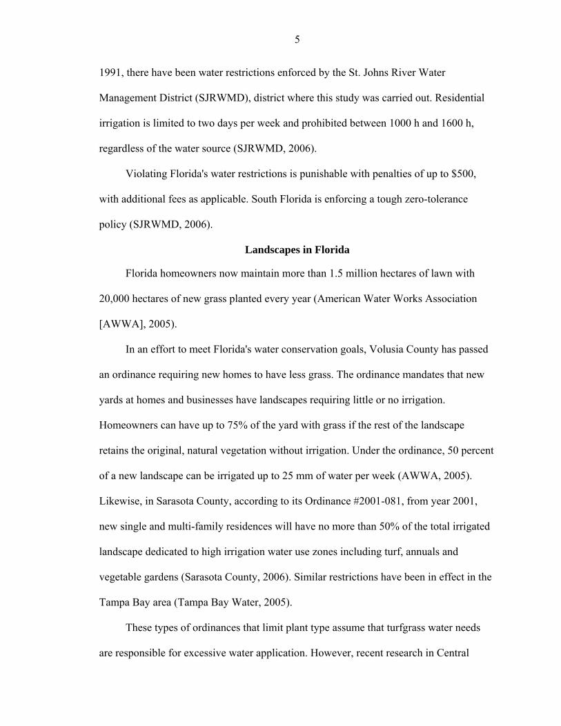
The simplest form of a CCL system is to set up a high-frequency irrigation in the
timer, which could be interrupted by a soil moisture sensor. The sensor is wired into the
line that supplies power from the timer to the electric solenoid valve (Figure 1-1). The
sensor operates as a switch that responds to soil moisture content. When sufficient soil-
moisture is available, the sensor maintains an open circuit between the timer and the
solenoid valve. When soil-moisture drops below a certain threshold, the sensing device
closes the circuit. Thus, the irrigation control system can bypass a pre-programmed
schedule, or maintain the soil water content within a specified range. These two
approaches are known as bypass and on-demand, respectively (Dukes and Muñoz-
Carpena, 2005). Bypass configurations skip an entire timed irrigation event based on the

8
soil water status at the beginning of that event or by checking the soil water status at
intervals within a time-based event (Muñoz-Carpena and Dukes, 2005).
Soil Moisture Content Measurement
The standard method of measuring soil moisture content is the thermogravimetric
method, which requires oven drying of a known volume of soil at 105 °C and
determining the weight loss. This method is time consuming and destructive to the
sampled soil, meaning that it cannot be used for repetitive measurements at the same
location. However, it is indispensable as a standard method for calibration and evaluation
purposes (Walker et al., 2004).
Among the widely used on-site soil moisture measurement techniques are neutron
scattering, gamma ray attenuation, soil electrical conductivity (including electrical
conductivity probes, electrical resistance blocks and electromagnetic induction),
tensiometry, hygrometry (including electrical resistance, capacitance, piezoelectric
sorption, infra-red absorption and transmission, dimensionally varying element, dew
point, and psychometric), and soil dielectric constant (including capacitance and time
domain reflectometry). Reviews on the advantages, disadvantages, and basis of these
measurement techniques may be found in Schmugge et al., 1980; Campbell and Mulla,
1990; Charlesworth, 2000; Ley et al., 2000; Topp, 2003; Muñoz-Carpena, 2004; and
Walker et al., 2004.
Granular matrix sensor
The granular matrix sensor (GMS) is a device that measures soil electrical
resistance, that can be converted to soil water tension (SWT), either using a calibration
formula provided in the literature for sandy soils (Irmak and Haman 2001) and silt loam
9
soils (Eldredge et al., 1993), or calibrating them for a specific soil type (Hanson et al.,
2000b; Intrigliolo and Castel, 2004).
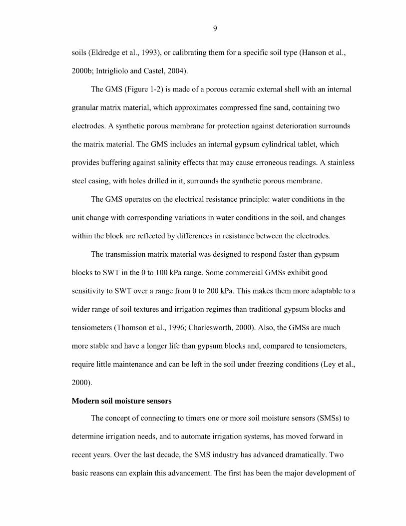
The GMS (Figure 1-2) is made of a porous ceramic external shell with an internal
granular matrix material, which approximates compressed fine sand, containing two
electrodes. A synthetic porous membrane for protection against deterioration surrounds
the matrix material. The GMS includes an internal gypsum cylindrical tablet, which
provides buffering against salinity effects that may cause erroneous readings. A stainless
steel casing, with holes drilled in it, surrounds the synthetic porous membrane.
The GMS operates on the electrical resistance principle: water conditions in the
unit change with corresponding variations in water conditions in the soil, and changes
within the block are reflected by differences in resistance between the electrodes.
The transmission matrix material was designed to respond faster than gypsum
blocks to SWT in the 0 to 100 kPa range. Some commercial GMSs exhibit good
sensitivity to SWT over a range from 0 to 200 kPa. This makes them more adaptable to a
wider range of soil textures and irrigation regimes than traditional gypsum blocks and
tensiometers (Thomson et al., 1996; Charlesworth, 2000). Also, the GMSs are much
more stable and have a longer life than gypsum blocks and, compared to tensiometers,
require little maintenance and can be left in the soil under freezing conditions (Ley et al.,
2000).
Modern soil moisture sensors
The concept of connecting to timers one or more soil moisture sensors (SMSs) to
determine irrigation needs, and to automate irrigation systems, has moved forward in
recent years. Over the last decade, the SMS industry has advanced dramatically. Two
basic reasons can explain this advancement. The first has been the major development of

10
computer technology (with more powerful, smaller and economical integrated circuits).
The other phenomenon has been the significant advances in the application of
electromagnetic methods to the measurement of soil water content. These methods make
use of the high relative permittivity (dielectric constant) of the water in soil for estimating
the water content. The relative permittivity of water is about 80, whereas the other
components in soil, including air, have relative permittivities in the range of one to seven.
Hence, methods that measure the relative permittivity are effective for the measurement
of soil water content (Topp, 2003).
Combining the computer technology and the soil dielectric concept has allowed
manufacturers to produce a number of different types of inexpensive SMSs for irrigation
scheduling. An increasing adoption of the dielectric methods has been observed, because
they are non-destructive, provide almost instantaneous measurements, do not require
maintenance, and can provide continuous readings through automation. However, they
have important differences in terms of calibration requirements, accuracy, cost,
installation and maintenance requirements, etc. (Muñoz-Carpena and Dukes, 2005).
The main techniques used by these sensors can be classified as Time Domain
Reflectometry (TDR) and Frequency Domain Reflectrometery (FDR) (Leib et al., 2003).
Time domain reflectometry. The speed of an electromagnetic signal passing
through a material varies with the dielectric of the material. Most TDR instruments
operate by sending a step pulse signal down steel rods (called wave-guides) buried in the
soil. The signal reaches the end of the probes and is reflected back to the TDR control
unit where it is detected and analyzed. The time taken for the pulse to return varies with
11
the soil dielectric, which is related to the water content of the soil surrounding the probe
(Topp, 2003).
According to Charlesworth (2000) and Edis and George (2000), TDR instruments
give the most robust soil water content data, with little need for recalibration between
different soil types. An important advantage of TDRs in turfgrass irrigation management,
is that accurate measurements may be made near the surface compared to techniques such
as the neutron probe (Ley et al., 2000).
Frequency Domain Reflectometry. Frequency domain reflectometry (FDR)
measures the soil dielectric by placing the soil (in effect) between two electrical plates to
form a capacitor. Hence ‘capacitance’ is the term commonly used to describe what these
instruments measure. When a voltage is applied to the electric plates a frequency can be
measured. This frequency varies with the soil dielectric (Charlesworth, 2000).
In spite of the advances and advantages of these modern SMSs, when comparing
the performance of different brand/types, significant differences were found in respect to
set-up requirements, accuracy, data interpretation, maintenance, and initial cost (Ley et
al., 2000) and the ability to repeat measurements accurately over time and under various
moisture regimes after initial calibration (Yoder et al., 1998).
Controllers
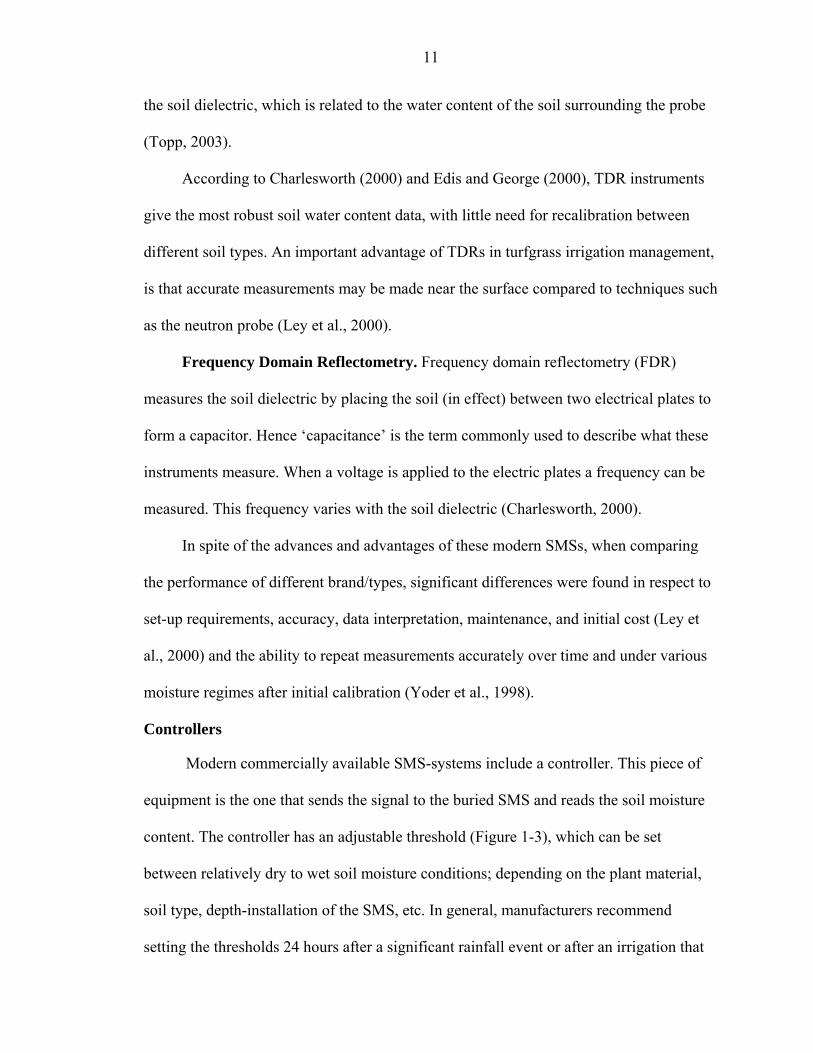
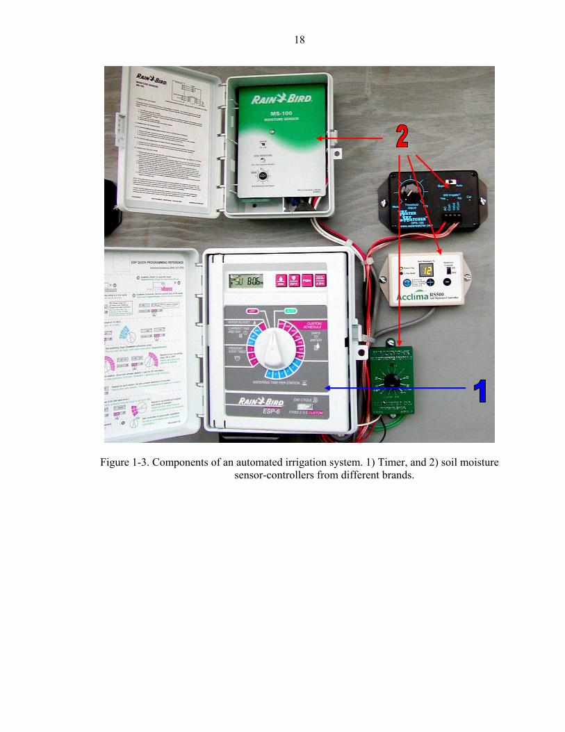
Modern commercially available SMS-systems include a controller. This piece of
equipment is the one that sends the signal to the buried SMS and reads the soil moisture
content. The controller has an adjustable threshold (Figure 1-3), which can be set
between relatively dry to wet soil moisture conditions; depending on the plant material,
soil type, depth-installation of the SMS, etc. In general, manufacturers recommend
setting the thresholds 24 hours after a significant rainfall event or after an irrigation that

12
filled the soil profile with water to field capacity. The controller is connected in series
with the residential irrigation timer and acts as a switch depending on the pre-set soil
moisture threshold.
Automatic Control of Irrigation
An automatic SMS-based irrigation system seeks to maintain a desired soil
moisture range in the root zone that is optimal or adequate for plant growth and/or
quality. This type of system adapts the amount of water applied according to plant
requirements without managers having to undertake daily monitoring or make
adjustments according to actual weather conditions (Muñoz-Carpena and Dukes, 2005;
Pathan et al., 2003).
The continuous monitoring of the soil moisture status becomes particularly
important in sandy soils. A wide range of applications to automatically control irrigation
events has been investigated in coarse textured soils. In Florida, switching tensiometers
have been studied for agricultural production (Smajstrla and Koo, 1986, Clark et al.,
1994; Smajstrla and Locascio, 1994; Muñoz-Carpena et al., 2003, Muñoz-Carpena et al.,
2005), and for maintaining bermudagrass turf (Augustin and Snyder, 1984). Although
they found water savings, these investigations suggest that tensiometers require
calibration and frequent maintenance, up to twice per week. Consequently, the adoption
of this technology will not lead to automatically controlled irrigation since it will not
eliminate human interaction in irrigation management.
Other types of sensors have been adapted to automate irrigation based on soil
moisture status. Nogueira et al. (2002) used TDR sensors to maintain soil moisture within
two preset limits (upper and lower soil moisture thresholds). Dukes and Scholberg (2005)
and Dukes et al. (2003) found 11% and 50% in water savings, without diminishing yields

13
on sweet corn and green bell pepper, using TDR probes and a commercially available
dielectric sensor, respectively. Granular matrix sensors (GMSs) have also been used to
automatically irrigate agricultural products (Muñoz-Carpena et al., 2003; Shock et al.,
2002) and, as with other solid-state sensors, do not require as much maintenance as
tensiometers. Although TDR and GMS, as well as similar types of sensors, have been
successfully used in agriculture, they have found limited use in residential landscape
irrigation (Qualls et al., 2001).
Rain Sensors
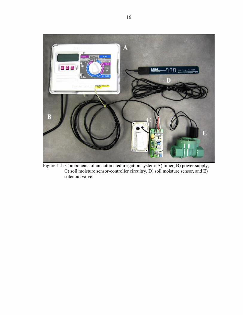
A rain sensor (RS), also called rain shut-off device (Figure 1-4), is a piece of
equipment designed to interrupt a scheduled cycle of an automatic irrigation system
controller when a specific amount of rainfall has occurred and, depending on the weather
conditions, after the said rainfall (Dukes and Haman, 2002b; Hunter Industries Inc.,
2006).
Florida law requires a RS device on all automatic lawn sprinkler systems (Florida
Statutes, Chapter 373.62, n.d.). The original text said: “Any person who purchases and
installs an automatic lawn sprinkler system after May 1, 1991, shall install a rain sensor
device or switch which will override the irrigation cycle of the sprinkler system when
adequate rainfall has occurred.” In 2001, this Chapter was amended to require the owner
not only to install, but also to maintain and operate a RS device or switch (Florida
Statutes, 2001). Moreover, some local laws also require older systems to be retrofitted
with rain shut-off switches (SJRWMD, 2006).
Florida is the only state in the nation with an overall RS statute. However, recently,
Georgia Gov. Sonny Perdue has signed into law H1277 requiring RSs on newly installed

14
irrigation systems in the Atlanta metro region. The new law affects systems installed after
January 1, 2005 (AWWA, 2004).
As with soil moisture sensors, rain sensors can be connected to any automatic
irrigation system controller and mounted in an open area where they are exposed to
rainfall. The new irrigation timers have a special connection, which allows a RS to be
attached directly. If it is not available, or the sensor does not work with a given timer, the
sensor can always be “hard-wired” into the controller, wiring the RS in series with the
common wire. When a specific amount of rainfall has occurred, the RS will interrupt the
irrigation system common wire, which disables the solenoid valves until the sensor dries
(Dukes and Haman, 2002b).
Figure 1-4 shows a simple and low cost RS. Rain causes the hygroscopic porous
disks in the device to swell and open a micro-switch (Figure 1-5). The switch remains
open as long as the disks are swollen. When the rain has passed and the disks dry out, the
switch will close again.
According to Dukes and Haman (2002b), the use of rain sensors has several
advantages: they conserve water, preventing irrigation after recent rain events; reduce
wear on the irrigation system, because the system runs only when necessary; reduce
disease and weeds development, by eliminating unnecessary irrigation events; help
protect surface and groundwater, by reducing the runoff and deep percolation that carries
pollutants, such as fertilizers and pesticides; and, finally, RSs save money, because they
reduce utility bills and maintenance costs.
Rain sensors should be mounted on any surface where they will be exposed to
unobstructed rainfall, but should not be in the path of sprinkler spray. These sensors are

15
typically installed near the roofline on the side of a building, but manufacturers
recommend mounting it in a location that receives about the same amount of sun and
shade as the turf (Hunter Industries Inc., 2006).
Irrigation and Turfgrass Quality
Under-irrigation and over-irrigation can negatively affect turfgrass quality. It has
been reported that, deeper and reduced irrigation frequency improves turfgrasses quality.
Augustin and Snyder (1984) concluded that this practice tends to reduce N leaching in
sandy soils, increasing N utilization, resulting in a better color rating (better quality).
Bonos and Murphy (1999) reported an increase in a Kentucky bluegrass (Poa pratensis
L.) cultivar root growth as drought stress was imposed. Recently, Jordan et al. (2003)
found that bentgrass irrigated every 4 days produced a significantly denser and deeper
root system, a higher shoot density, and greater overall plant health, resulting in better
turf quality, than grass watered every 1 or 2 days (even under putting green management
conditions). McCarty (2005) summarizes that drier conditions slow shoot growth and
increase root growth and leaf water content.
Moreover, limitations to establishment and survival of some turfgrass weeds
(Colbaugh and Elmore, 1985; Youngner et al., 1981), and reduction of some pathogens
severity (Davis and Dernoeden, 1991; Kackley et al., 1990) has been associated with
deep, infrequent irrigation.
16
Figure 1-1. Components of an automated irrigation system: A) timer, B) power supply,
C) soil moisture sensor-controller circuitry, D) soil moisture sensor, and E) solenoid valve.

17
Figure 1-2. Granular matrix sensors (GMS)
18
Figure 1-3. Components of an automated irrigation system. 1) Timer, and 2) soil moisture sensor-controllers from different brands.

19
Figure 1-4. Rain shut-off switch.
Figure 1-5. The expanding material of a rain shut-off switch.

20
CHAPTER 2 SENSOR-BASED AUTOMATION OF IRRIGATION OF BERMUDAGRASS
Introduction
Turfgrass in landscape applications is the most extensively cultivated crop in
Florida (Hodges et al., 1994; USDA, 2005). Irrigation of residential, industrial,
commercial, and recreational turf areas is commonly employed to ensure acceptable turf
quality. As a consequence of problems related to drought, coupled with a steadily
increasing demand for water, the state of Florida has imposed restrictions on irrigation
water use. The development of Best Management Practices (BMPs) for irrigation water
use in turf has become an undeniable strategic, economic, and environmental issue for the
state. New irrigation technologies could improve irrigation efficiency promoting water
conservation and reducing the environmental impacts of the landscapes, which are often
composed of turfgrass as a major portion of the irrigated area.
Florida receives an average of around 1400 mm of rainfall a year, which typically
exceeds evapotranspiration. Nevertheless, irrigation is required because total annual
rainfall for Florida typically varies both geographically and temporally (USDA, 1981;
Carriker, 2000; NOAA, 2003), and lack of rainfall for even a few days causes depletion
of moisture in Florida's predominately sandy soils (Carriker, 2000; National Research
Council, 1996).
Florida has the second largest withdrawal of groundwater for public supply in the
United States. In 1995, nearly 93% of population in Florida used groundwater as a
drinking water source (Solley et al., 1998). Florida has a fast-growing population with a

21
net inflow of more than 1100 people a day. By 2025, it is projected to be the third most
populous state in the nation (Office of Economic and Demographic Research [ODR],
2006; USCB 2004a). The U.S. Census Bureau estimated that Florida accounted for
approximately 11% of all new homes constructed in the U.S. in 2003, the largest amount
in any single state in the U.S. (USCB, 2004b), the majority of them with in-ground
irrigation systems1 (Tampa Bay Water, 2005). As urban populations swell, pressures on
limited supplies of clean water are increasing. Even saltwater intrusion in groundwater
from the Floridan aquifer have been found in coastal Hillsborough, Manatee and Sarasota
counties (Southern Water Use Caution Area Recovery Strategy [SWUCA], 2006)
The primary use of residential outdoor water is irrigation. Recent studies in the
U.S. indicate that, on average, 58% of potable water is used for landscape irrigation, that
households that use automatic timers to control their irrigation systems used 47% more
water outdoors than those without timers, and that homes with in-ground sprinkler
systems use 35% more water outdoors than those without in-ground systems (Mayer et
al., 1999). In the Central Florida Ridge, the potable water used for landscape irrigation is
as high as 74%, with an average of 64% (Haley et al., 2006), and even when irrigation is
restricted to two days a week and from 1000 h to 1600 h (SJRWMD, 2006), typically
homeowners tended to over-irrigate (Haley et al., 2006).
Over-irrigation or under-irrigation can negatively affect turfgrass quality. It has
been reported that deeper and reduced irrigation frequency improves turfgrass quality.
Augustin and Snyder (1984) concluded that this practice tended to reduce N leaching in
1 57% and 85% of new homes built in Pasco and Hillsborough counties, respectively, have in-ground irrigation systems. Actual percentages may be higher since many homeowners install irrigation systems after moving into the home. In the Tampa region, 70% of homes are estimated to have in-ground irrigation.

22
sandy soils, increasing N utilization, resulting in a better color rating (better quality).
Bonos and Murphy (1999) reported an increase in a Kentucky bluegrass (Poa pratensis
L.) cultivar root growth as drought stress was imposed. Recently, Jordan et al. (2003)
found that bentgrass irrigated every 4 days produced a significantly larger and deeper root
system, a higher shoot density, and an overall plant health–resulting in greater turf
quality–than that watered every 1 or 2 days (even under golf putting green management
conditions). McCarty (2005) summarizes that drier conditions slow shoot growth, and
increase root growth and leaf water content. Moreover, limitations to the establishment
and survival of some turfgrass weeds (Colbaugh and Elmore, 1985; Youngner et al.,
1981), and reduction of some pathogens severity (Davis and Dernoeden, 1991; Kackley
et al., 1990) have been associated with deep, infrequent irrigation. Hence, better irrigation
scheduling by homeowners may lead to improved turfgrass quality coupled with potential
savings in irrigation water use.
Over the last decade, the soil moisture sensor (SMS) industry has advanced
dramatically. Two basic reasons can explain this advancement. The first has been the
major development of computer technology (with more powerful, smaller and more
economical integrated circuits), and the other phenomenon has been the significant
advances in the application of electromagnetic methods to the measurement of soil water
content. These methods make use of the high relative permittivity (dielectric constant) of
the water in soil for estimating the water content. The relative permittivity of water is
about 80, whereas the other components in soil, including air, have relative permittivities
in the range of one to seven. Hence, methods that measure the relative permittivity are
effective for the measurement of the soil water content (Topp, 2003).

23
Combining the computer technology and the soil dielectric concept has allowed
manufacturers to design and produce a number of different types of inexpensive SMSs
for irrigation scheduling. However, when comparing the performance of different
brand/types of sensors for measurement of soil moisture, differences were found. For
example, Ley et al. (2000) found significant differences between sensors with respect to
set-up requirements, accuracy, data interpretation, maintenance, and initial cost. Yoder et
al. (1998) obtained differences related with error, accuracy, reliability, durability,
installation factors, and the ability to repeat measurements accurately over time and under
various moisture regimes after initial calibration.
Automation of irrigation systems, based on SMSs, has the potential to provide
maximum water use efficiency, by maintaining soil moisture between a desired range that
is optimal or adequate for plant growth and/or quality; allowing irrigation only when
necessary (Muñoz-Carpena and Dukes, 2005).
A wide range of applications to automatically control irrigation events have been
investigated in coarse textured soils. In Florida, switching tensiometers have been studied
for agricultural production (Smajstrla and Koo, 1986, Clark et al., 1994; Smajstrla and
Locascio, 1994; Muñoz-Carpena et al., 2003; Muñoz-Carpena et al., 2005), and for
maintaining bermudagrass turf (Augustin and Snyder, 1984). Although they found water
savings, these investigations suggest that tensiometers require calibration and frequent
maintenance, up to twice per week. Consequently, the adoption of this technology will
not lead to an automatically controlled irrigation system, since it will not eliminate
human interaction in irrigation management.
24
Other types of sensors have been adapted to automate irrigation based on soil
moisture status in Florida. Nogueira et al. (2002) used TDR sensors to maintain soil
moisture within two preset limits (upper and lower soil moisture thresholds). Dukes and
Scholberg (2005) and Dukes et al. (2003) found 11% and 50% in water savings–without
diminishing yields–using TDR probes on sweet corn, and a commercially available
dielectric sensor on green bell pepper, respectively. Granular matrix sensors (GMSs)
have also been used to automatically irrigate agricultural products (Muñoz-Carpena et al.,
2003; Shock et al., 2002) and, as with other solid-state sensors, do not require as much
maintenance as tensiometers.
Although SMSs have been successfully used in agriculture, they have found limited
use in residential landscape irrigation and further investigation is required to provide
evidence of their potential use in this area. A study using GMSs to control urban
landscape irrigation in Colorado, used 533 mm of water for irrigation when compared to
the theoretical requirement of 726 mm, a reduction of 27% (Qualls et al., 2001).
Since 1991, Florida law requires a rain sensor device or switch hooked up to all
automatic lawn sprinkler systems (Florida Statutes, Chapter 373.62, n.d.). A rain sensor
(RS) is a piece of equipment designed to interrupt a scheduled cycle of an automatic
irrigation system controller when a specific amount of rainfall has occurred (Dukes and
Haman, 2002b; Hunter Industries Inc., 2005). Benefits and advantages of its use are
similar to those of SMSs, and have been summarized by Dukes and Haman (2002b).
Even when this law has been in effect for a long time, and RSs have been commercially
available for many years, little evidence related to their usefulness and/or to quantify their
water savings exists

25
The goals of this research were to find out if different SMS-systems (sensor with a
proprietary controller) could reduce irrigation water application–while maintaining
acceptable turf quality–compared to current practices. The objectives of this experiment
were to quantify differences in irrigation water use and turf quality between: 1) a SMS-
based irrigation system compared to a time-based scheduling, 2) different commercial
irrigation SMSs, and 3) a time-based scheduling system with or without a RS.
Materials and Methods
The experimental area was located at the Agricultural and Biological Engineering
Department facilities, University of Florida, Gainesville, Florida; on an Arredondo fine
sand (loamy, siliceous, semiactive, hyperthermic Grossarenic Paleudults) (Thomas et.al,
1985; USDA, 2003). This soil has a field capacity of 7% (Figure 2-1), as determined
from repacked soil columns (see Chapter 4 for methodology details).
Seventy-two 3.66 m x 3.66 m plots were established on a field covered with
common bermudagrass (Cynodon dactylon L.). Each plot was sprinkler irrigated by four
quarter-circle pop-up spray heads, with an application rate of 38 mm/hr and regulated at
172 kPa (Hunter 12A, Hunter Industries, Inc., San Marcos, CA). Much of the irrigation
hardware was in place from a previous research project; however, extensive renovations
were performed to make the equipment serviceable.
Plots were mowed twice weekly at a height of 5.5 cm. Chemicals were applied as
needed to control weeds and pests. Nutrient applications were made using ammonium
sulfate (21-0-0), at a N rate of 50 kg ha-1, on April and May of 2004, before the beginning
26
of the experiment. Then, a granulated N controlled-release fertilizer (Polyon, PTI,
Sylacauga, AL) 2 was applied at a rate of 180 kg ha-1, on July 2004 and April 2005.
Four commercially available SMSs were selected for evaluation (Figure 2-2):
Acclima Digital TDT RS-500 (Acclima Inc., Meridian, ID), Watermark 200SS-5
(Irrometer Company, Inc., Riverside, CA), Rain Bird MS-100 (Rain Bird International,
Inc., Glendora, CA), and Water Watcher DPS-100 (Water Watcher, Inc., Logan, UT),
codified as AC, IM, RB, and WW, respectively. In order to find similar outcomes to
those that homeowners would encounter, sensors were not calibrated, and were used
directly “out of the box.”
Each one of these SMSs systems includes a SMS and a controller (Figure 2-3). The
controller’s thresholds can be adjusted between “dry” and “wet” on the RB (on a 1 to 8
scale), and between “moist” and “dry” on the WW (on a -3 to 3 scale). The IM can be set
at a specific soil water tension (kPa) and the AC can be set directly to a specific soil
volumetric moisture content (VMC), expressed in percent.
As recommended by manufacturers, all controller thresholds, except for the AC,
were set 24 hours after a significant rainfall event (on 20 July 2004, after four days of
rain with a total of 107 mm) that filled the soil profile with water. On RB controllers, the
thresholds were set by adjusting the dial until the LED turned off and on. On the WW,
initially the unit could not be calibrated since the soil moisture was outside the range of
the controller. After discussion with the manufacturer, a resistor was added between the
solenoid valve wire and the valve common wire. The calibration procedure consisted of
activating the reset button, which allowed its auto-calibration. The IM controller was set 2 The mention of trade and company names is for the benefit of the reader and does not imply an endorsement of the product.

27
at number 1 (equivalent to 10 kPa, and approximately to field capacity, according to the
manufacturer), whereas the AC controller was set on their display at a VMC of 7%, based
on the measured soil water release curve of the soil. All these controllers were connected
in series with typical residential irrigation timers (see description of timers under
Treatments sub-heading).
Treatments
Two basic types of treatments were defined: SMS-based treatments, and time-based
treatments (Table 2-1). In the SMS-based treatments, all four brands were tested with
three irrigation frequencies: one, two, and seven days per week (1 d/w, 2 d/w and 7 d/w,
respectively). The 1 d/w and 2 d/w watering frequencies represent typical watering
restrictions imposed in Florida (FDEP, 2002; SJRWMD, 2006).
Within the time-based treatments, a frequency of 2 d/w was defined (the most
common in Florida, and current watering restriction in the area of study). Two treatments
were connected to a rain sensor (2-WRS and 2-DWRS), to simulate requirements
imposed on homeowners by Florida Statutes (Chapter 373.62, n.d.). The rain sensor
(Figure 2-4) (Mini-click II, Hunter Industries, Inc., San Marcos, CA) was set at 6 mm
rainfall threshold. A without-rain-sensor treatment (2-WORS) was also included, in order
to simulate homeowner irrigation systems with an absent or non-functional rain sensor.
Finally, a non-irrigated treatment (0-NI) was also implemented as a control for turfgrass
quality. All experimental treatments were repeated four times, for a total of 64 plots, in a
modified completely randomized design3.
3 See Dry-Wet Analysis subheading for details
28
The weekly irrigation depth was set to replace the historical ET-based irrigation
schedule recommended by Dukes and Haman (2002a) for the area where this experiment
was carried out (Table 2-2). All treatments were programmed to have the equal
opportunity to apply the same amount of irrigation per week, except for treatments 2-
DWRS (deficit-with-rain-sensor, 60% of this amount), and 0-NI (non-irrigated). The
irrigation depths were adjusted monthly.
The irrigation cycles were programmed on two ESP-6, and three ESP-4Si model
timers (Rain Bird International, Inc., Glendora, CA) (Figure 2-3). They were
programmed to start between 0100 and 0500 h, with the purpose of diminishing wind
drift and decreasing evaporation.
Uniformity Test
An irrigation uniformity test measures the relative distribution application of water
depth over a given area. This concept results in a numeric value to quantify the variability
in depth of sprinkler irrigation over a target area. Two methods have been developed to
quantify uniformity: distribution uniformity (DU) and Christiansen’s coefficient of
uniformity (CU).
According to Merriam and Keller (1978), the low-quarter irrigation distribution
uniformity (DUlq) can be calculated with the following equation:
tot
lqlq D
DDU = [2-1]
where lqD is the lower quarter of the average of a group of catch-can measurements, and
totD is the total average of a group of catch-can measurements. This method emphasizes
the areas that receive the least irrigation by focusing on the lowest quarter. Although a
29
system may have even distribution, over-irrigation can occur because of mismanagement
(Burt et al., 1997).
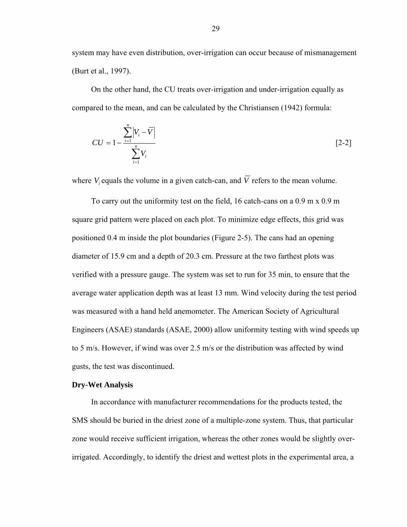
On the other hand, the CU treats over-irrigation and under-irrigation equally as
compared to the mean, and can be calculated by the Christiansen (1942) formula:
∑
∑
=
=
−−= n
ii
n
ii
V
VVCU
1
11 [2-2]
where iV equals the volume in a given catch-can, and V refers to the mean volume.
To carry out the uniformity test on the field, 16 catch-cans on a 0.9 m x 0.9 m
square grid pattern were placed on each plot. To minimize edge effects, this grid was
positioned 0.4 m inside the plot boundaries (Figure 2-5). The cans had an opening
diameter of 15.9 cm and a depth of 20.3 cm. Pressure at the two farthest plots was
verified with a pressure gauge. The system was set to run for 35 min, to ensure that the
average water application depth was at least 13 mm. Wind velocity during the test period
was measured with a hand held anemometer. The American Society of Agricultural
Engineers (ASAE) standards (ASAE, 2000) allow uniformity testing with wind speeds up
to 5 m/s. However, if wind was over 2.5 m/s or the distribution was affected by wind
gusts, the test was discontinued.
Dry-Wet Analysis
In accordance with manufacturer recommendations for the products tested, the
SMS should be buried in the driest zone of a multiple-zone system. Thus, that particular
zone would receive sufficient irrigation, whereas the other zones would be slightly over-
irrigated. Accordingly, to identify the driest and wettest plots in the experimental area, a

30
survey was carried out on each plot, before the beginning of the experiment. In addition,
because a total of 64 plots were required, this analysis was used to discard 8 plots from a
pool of 72 plots available.
On 12 March 2004, after 14 days without rainfall, a relatively “dry” soil moisture
condition was evident. The VMC was measured in each plot by means of a hand held
TDR device, which measured the moisture in the top 20 cm (Field Scout 300, Spectrum
Technologies, Inc., Plainfield, IL). Measurements were taken at five locations in the
center 1 m X 1 m of each plot and averaged. On 17 March 2004, 24 hr after a 23 mm
rainfall filled the soil profile, the VMC on a “wet” condition was measured as well. After
selecting the driest plots, the SMS that controlled a particular treatment was buried in the
center of one of these plots, thereby controlling all four replications. In all cases, SMSs
were installed in the top 7-10 cm of the soil, where most of the roots were present.
Plot Irrigation Management and Data Collection
Figures 2-6 to 2-10 show the set up of the different control features of the
experiment. Each plot was managed individually, and data were collected independently
from each plot as well. Pulse-type positive displacement flowmeters (PSMT 20mm x
190mm, Amco Water Metering Systems, Inc., Ocala, FL) were connected to nine
AM16/32 multiplexers (Campbell Scientific, Logan, UT), which were hooked up to a CR
10X model datalogger (Campbell Scientific, Logan, UT), to continually measure
irrigation volume and frequency applied to each plot (Figure 2-10). In addition, meters
were read manually each week.
Weather data were collected by an automated weather station (Campbell Scientific,
Logan, UT), located within 1 m of the experimental site (Figure 2-11). Measurements,
made every fifteen minutes, included air temperature, relative humidity, wind speed,

31
wind direction, solar radiation, barometric pressure, and soil heat flux. Rainfall was
recorded continuously by a manual rain gauge during 2004 and by a tipping bucket rain
gauge in 2005.
Reference evapotranspiration (ETo) was calculated from the Penman–Monteith
equation described in FAO-56 (Allen et al., 1998) as follows:
ETo
( ) ( )( )2
2
34.01273
900408.0
u
eeuT
GR asn
++∆
−+
+−∆=
γ
γ [2-5]
∆ = ( )23.237
3.23727.17exp6108.04098
+
⎥⎦
⎤⎢⎣
⎡⎟⎠⎞
⎜⎝⎛
+
TT
T
[2-6]
Rn = Rns - Rnl [2-7]
Rnl = ( ) ⎟⎟⎠
⎞⎜⎜⎝
⎛−−
⎥⎥⎦
⎤
⎢⎢⎣
⎡ +35.035.114.034.0
2
4min,
4max,
so
sa
KK
RRe
TTσ [2-8]
Rns = (1- α)Rs [2-9]
Rso = (0.75 + z(2 x 10⁻⁵))Ra [2-10]
Ra = [ ])cos()cos()sin()sin()sin()60(24 δϕωδϕωπ ssrscdG + [2-11]
dr = 1 + 0.033 cos ⎟⎠⎞
⎜⎝⎛ J
3652π [2-12]
δ = 0.409 sin ⎟⎠⎞
⎜⎝⎛ − 39.1
3652 Jπ [2-13]
ωs = arcos [-tan(ϕ)tan(δ)] [2-14]
es = 2
)(Te )(Te mino
maxo + [2-15]
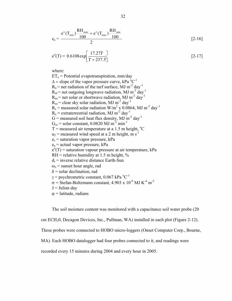
32
ea = 2
100RH)(Te
100RH)(Te min
maxomax
mino +
[2-16]
eo(T) = ⎥⎦⎤
⎢⎣⎡
+ 3.23727.17exp6108.0
TT [2-17]
where: ETo = Potential evapotranspiration, mm/day ∆ = slope of the vapor pressure curve, kPa oC-1 Rn = net radiation of the turf surface, MJ m-2 day-1 Rnl = net outgoing longwave radiation, MJ m-2 day-1 Rns = net solar or shortwave radiation, MJ m-2 day-1 Rso = clear sky solar radiation, MJ m-2 day-1 Rs = measured solar radiation W/m2 x 0.0864, MJ m-2 day-1 Ra = extraterrestrial radiation, MJ m-2 day-1 G = measured soil heat flux density, MJ m-2 day-1 Gsc = solar constant, 0.0820 MJ m-2 min-1 T = measured air temperature at a 1.5 m height, oC u2 = measured wind speed at a 2 m height, m s-1 es = saturation vapor pressure, kPa ea = actual vapor pressure, kPa eo(T) = saturation vapour pressure at air temperature, kPa RH = relative humidity at 1.5 m height, % dr = inverse relative distance Earth-Sun ωs = sunset hour angle, rad δ = solar declination, rad γ = psychrometric constant, 0.067 kPa oC-1 σ = Stefan-Boltzmann constant, 4.903 x 10⁻⁹ MJ K-4 m-2 J = Julian day ϕ = latitude, radians
The soil moisture content was monitored with a capacitance soil water probe (20
cm ECH20, Decagon Devices, Inc., Pullman, WA) installed in each plot (Figure 2-12).
These probes were connected to HOBO micro-loggers (Onset Computer Corp., Bourne,
MA). Each HOBO datalogger had four probes connected to it, and readings were
recorded every 15 minutes during 2004 and every hour in 2005.
33
Before the beginning of the experiment, calibration of the ECH2O probes was
performed at the research site using the thermogravimetric soil sampling method
(Gardner, 1986). Four probes connected to a HOBO datalogger were installed in the field.
Undisturbed soil samples were collected from the field at less than 20 cm from the
probes, and at the same depth where the probes were placed. Samples were taken from a
saturated through a dry condition. When each sample was removed, date and time was
recorded. The volumetric soil water content of each sample was then compared to the
ECH2O probe readings at the same date and time when the samples were taken (see
Chapter 4 for methodology details) and a site-specific calibration curve was developed.
Turfgrass quality was visually assessed and rated using a scale of 1 to 9, where 1
represents brown, dormant or dead turf, and 9 represents the best quality (Skogley and
Sawyer, 1992). A rating of 5 was considered the minimum acceptable turf quality for a
homeowner. Ratings were carried out in July, October and December of 2004, and in
April, May and July of 2005.
The data were obtained from 20 July through 14 December of 2004–when the
turfgrass went dormant due to cool temperatures, and irrigation was discontinued–and
from 25 March through 31 August of 2005.
Data Analysis
Statistical data analyses were performed using the general linear model (GLM)
procedure of the Statistical Analysis System software (SAS, 2000). Analysis of Variance
was used to determine treatment differences and Duncan's Multiple Range Test was used
to identify mean differences. The combined data from both years were analyzed. When
interactions between years and other parameters were detected, each year's data were
analyzed separately and, when needed, a monthly data analysis was made as well.
34
Results and Discussion
Uniformity Tests
The uniformity tests resulted in a wide range of DUlq values across the plots (15%
to 78%), with an average of 52% that, according to the Irrigation Association (2003)
overall system quality ratings, is considered “fair.” Obvious problems such as leaks and
broken heads were repaired prior to testing, but in some cases problems were discovered
as a result of testing (Figure 2-13, plots A8, A12, B9, and D1) and action was taken to
correct the problem. Baum et al. (2003) performed uniformity tests on irrigation systems
of homes in Central Florida having spray heads. That research found an average DUlq of
41%, with a range of 12% to 67%.
The average CU for all the plots was 71%, with a range of 50% to 89%. Baum et al.
(2003), found a CU average of 59%, with a range between 50% and 72%. Therefore,
these experimental plots had a better distribution application of water depth, expressed as
DUlq and CU, than actual spray irrigation zones on homes sampled in Central Florida.
It is interesting to mention that, considering all the catch-cans of the experiment
responsible for the lowest readings, 99% of them were placed on the edges of the plots,
indicating that substantial edge effects occurred in the testing. This is common for
sprinkler irrigation systems and did not negatively impact the results, because soil
moisture and turf quality ratings of each plot were always taken inside this perimeter. In
addition, this situation tended to minimize the effect of irrigation overlapping between
plots.
Dry-Wet Analysis
The data collected during the dry-wet analysis are shown in Figures 2-14 and 2-15.
The statistical analysis (Appendix B, Dry) revealed that at the dry condition, plots A11

35
and A12 were similar, but had significantly higher VMC than the other plots. Under the
wet condition, again plots A11 and A12 were significantly different from the rest, also
having a higher VMC.
Therefore, plots A11 and A12 were discarded for this experiment because they
were too “wet” (Figures 2-14 and 2-15). On the other hand, plots A4, A5, A7, A8, F11,
and F12 were also discarded, because they appeared to have the lowest VMC values of
all plots, coupled with a comparatively lower turfgrass quality before the beginning of the
experiment. These discarded plots appear in red in the plot plans shown in Figures 2-14
and 2-15. Consequently, a total of 64 plots were left for this research. When a statistical
analysis was performed (Appendix B, Wet) with the 64 plots included, the only
significant difference was that F1 and E1 showed higher values at the wet condition than
the rest, so they were discarded as locations for SMS placement.
The green plots shown in Figures 2-14 and 2-15 were selected to bury the SMS for
the control plots, because they appeared to be similarly dry and on the dryer end, and
because of the practical convenience of burying the cables of the different SMS on the
same trench, at the same time, and closer to the control board (Figure 2-8). A statistical
analysis on these plots (Appendix B, Plots with SMS) indicated that they were not
statistically different (P>0.94). Figure 2-16 shows the plot plan containing all the
treatments and repetitions, in a modified completely randomized design, where the same
color depicts treatment repetitions (plots showing an X were the discarded ones).
Rainfall
Both 2004 and 2005 were rainy years (Figures 2-17 and 2-18), with high frequency
rainfall events and a large amount of cumulative precipitation, which is not uncommon in
this region. During 2004, a tropical storm and two hurricanes–Frances and Jeanne–passed

36
over the research area during the experiment, resulting in 159, 286, and 157 mm of
rainfall, respectively. Year 2005 broke all records for the number of hurricanes and
named tropical storms in U.S., but none of them directly hit the area where the
experiment was carried out.
Nonetheless, during the data collection period of 2005, 40% of the days had rainfall
events, with a considerable amount of precipitation, 732 mm, and an average of 135
mm/month (Figure 2-18). In the course of 2004, (Figure 2-17) even when it rained less
frequently, 31% of the days, the cumulative rainfall for the experimental period was even
larger, with 944 mm, and 190+ mm/month on average. However, most of this rainfall
(530 mm, or 56%) occurred during the tropical storm and the two hurricanes. If these
events were not considered, an average of 84 mm/month fell during 2004.
Figure 2-17 shows that in 2004 most of the rain fell during August and September
(793 mm), and the least rain fell in October and November (116 mm). A relatively “dry”
period occurred from 21 October to 24 November (35 days), with only two small rainfall
events of 1.5 and 2.5 mm. A similar situation happened in 2005 (Figure 2-18) during
April and May, when 223 mm fell over 17 rainfall events. On the other hand, June, July,
and August were rainier months with 478 mm on 44 rainfall events.
Irrigation Events
Figures 2-19 and 2-20 show the evolution of the cumulative number of irrigation
events allowed per treatment in 2004 and 2005, respectively. There were a greater
number of irrigation events as the irrigation frequency increased (Parts B vs. C vs. D,
from Figures 2-19 and 2-20). The treatment without-rain-sensor (2-WORS) was
programmed to run 2 d/w, independently of the weather and/or soils moisture conditions
and, as expected, irrigation cycles were not bypassed. However, to avoid possible damage

37
to the equipment, power was turned off and no data were collected from 26 September
through 30 September 2004, due to hurricane Jeanne. This is reflected on Figure 2-19,
Part A, when through these dates the slope of the curves looks horizontal (no irrigation
events). Nevertheless, this period was rainy and very short in proportion, so final results
should not be significantly affected.
Treatments 2-WRS and 2-DWRS were controlled by the same rain sensor and set
to run the same days so, not surprisingly, they overrode the same amount of irrigation
cycles, and only one line can be seen for both treatments (Figure 2-19, Part A).
In spite of this result, it is important to know what proportion of the scheduled
irrigation cycles (SIC) were finally overridden by the different treatments (Table 2-3).
The statistical analysis (P<0.0001) showed that, as expected, 2-WORS was different from
the rest of the treatments (overriding 0% of the SIC), and that 2-WRS and 2-DWRS were
not statistically different. These last two treatments bypassed 30% and 37% of the
possible irrigation events in 2004 and 2005, respectively, and more than a third as an
average for both seasons.
Regarding the SMS-based treatments, there was not a clear difference between
them, except for the IMs. Sensors from brands AC, RB, and WW, overrode significantly
more SIC than 2-WRS and 2-DWRS, ranging from 70% to 92% in total, and considering
all frequencies tested. The proportion of SIC overridden by IMs, however, ranged from
32% to 50% the first year, from 24% to 70% in 2005, and from 28% to 56% for both
years together.
In the first year, 2-IM overrode almost the same proportion of irrigation cycles than
the control 2-WRS (32% vs. 30%, respectively). In 2005, however, 2-IM was the only
38
treatment that resulted in more irrigation cycles than the control treatment, overriding
only 24% of the possible ones compared to 37% by 2-WRS. As a result, 2-IM was not
statistically different from 2-WRS. The other two IM treatments did not differ
statistically, but overrode more irrigation cycles compared to 2-WRS and less than the
rest of the SMS-based treatments. These results suggest that IMs, except for the said 2-
IM in 2005, would be able to respond to rainfall events at least in a similar proportion
than a rain sensor device set at 6 mm.
In order to corroborate the effectiveness of the SMSs, it was important to detect
when actual irrigation cycles occurred and how were they related to rainfall and
evapotranspiration conditions.
Figures 2-21 and 2-22 show the maximum weekly irrigation water requirement–or
weekly rainfall – ETo difference (RED)–for years 2004 and 2005, respectively. In 2004,
August and September had only one week each with a negative RED. However, after 2
October, eight of eleven weeks showed a negative RED. On the other hand, in 2005, it
can be seen that every month had at least one deficitary week. However, the longest
negative REDs happened in April, May, and July of 2005, with three, four, and two
consecutive weeks, respectively.
Table 2-4 shows the percent of irrigation cycles allowed by the SMS-based
treatments through the experimental months of 2004 and 2005. In 2004, on average, a
lesser amount of irrigation events were allowed in August and September (21% and 18%,
respectively) compared to October and November (44% and 46%, respectively). In 2005,
a greater proportion of irrigation cycles were allowed in April, May, and July (31% and
46%, and 24%, respectively), and a fewer proportion in June and August (13% and 17%,
39
respectively). These tendencies were concordant with the dryer/rainier periods and, when
correlating the monthly RED values and the percent of irrigation cycles allowed per
month, r values of –0.93 and –0.76 were found for 2004 and 2005, respectively (Table 2-
4).
Looking in detail, for 2004, ACs followed this tendency allowing fewer irrigation
cycles during the rainy months of August and September, and more cycles during the
dryer period between October and November. In the case of 1-AC, the only irrigation
cycles allowed occurred in November. 2-AC allowed less irrigation cycles on August and
September (22% and 11%) and more cycles during October and November (22% and
33%, respectively); the same tendency as 7-AC (10%, 0%, 3%, and 17%, for the same
months, respectively).
RBs also responded to this tendency on the 1 d/w and 7 d/w frequencies, allowing a
greater proportion of SIC to occur during the end of the year; but 2-RB did not follow
this, and actually run more cycles at the beginning and at the end of the year (33% vs.
22%), with no irrigation cycles during September and October.
A similar situation occurred with the IM treatments. The first and second half of the
season were clearly different for 1-IM (between 20% - 25% vs. 50% - 100% of the SIC,
respectively), and for 2-IM (33% vs. 100%, respectively). However, 7-IM showed a more
even conduct for the first three months (84%, 73%, 87%, respectively), and then dropped
down in November (23%).
Finally, for 2004, WW treatments were also more active at the end of the season,
allowing between 33% and 75% of the SIC (with the exception of 2-WW, on November,
with 11%), compared to 0% to 29% for the first two months.
40
During 2005, ACs also followed the dryer/wetter period’s tendency in every
frequency tested. In the case of 1-AC, it ran 50% and 75% of the possible times on April
and May (the driest months), and did not allow irrigations on June, July, and August (the
wetter months). On these same last three months, 2-AC and 7-AC treatments allowed no
more than 13% and 10% of the potential irrigation cycles respectively.
A similar situation happened with WW sensors. No irrigation cycles were allowed
during the rainy months of June, July, and August by the 1 and 2 d/w frequencies. In the
case of 7-WW, it followed this tendency in June and August (with 10% and 6%,
respectively), but in July–month that had two consecutive weeks of negative RED–it
showed a higher number of irrigation events (32%).
In 2005, RB sensors allowed few irrigation cycles to start during all the different
months. The 1 d/w frequency permitted between 20 and 25% of the SIC, the 2 d/w
frequency resulted in 11%, and 7 d/w frequency between 6% and 19%. Nevertheless, all
the frequencies had a month when they did not allow any irrigation cycles (April, June,
and August for 1, 2, and 7 d/w, respectively).
IM, in general, permitted more irrigation cycles than the other sensors. The 1-IM
treatment showed similar behavior to the other brands during April, May, and June.
Nevertheless, during July and August, 60% and 75% of irrigation events were allowed,
respectively. Even in the rainy months of June, July, and August, 2-IM allowed 75% to
89% of the potential irrigation cycles to occur. A smaller variation in the number of
irrigation events allowed between the different months was shown by 7-IM (from 16% to
45%), and exhibited a closer pattern to the other brands, being more active in the months
41
of April and May. However, it also permitted a greater amount of irrigation cycles per
month than the other brands at this frequency.
These relationships are clearer when looking at the VMC of the plots for year 2004,
when evident differences in weather conditions through time were found. Figure 2-23
shows the VMC of treatment 0-NI where all the increments in VMC were due to rainfall
events. The differences between the dry and the wet periods were reflected in the soil
moisture content. Figures 2-24 to 2-35 show the VMC in plots that contained the SMSs
controlling the irrigation treatments. These figures, show the results of the scheduled
irrigation cycles (SIC), where the blue dots represent bypassed SIC, the red dots represent
allowed SIC, and the red lines represent the range of VMC when the SIC were allowed.
When an increment in the VMC does not have a red dot, it means that a rainfall event
occurred.
These results show that, in general, the SMS-based treatments were able to follow
the dryer and wetter periods, controlling the amount of water to be delivered to the
different treatments, and suggesting that this technology could be a useful tool to achieve
automation of landscape-turfgrass irrigation, even when a RS is not present or non-
functional. However, these are not precision instruments, which was evident because
sometimes they bypassed irrigation cycles, and sometimes they did not, even reading the
same or lower VMC. Moreover, according to the range of VMC over which the different
SMS brands allowed irrigation, AC and RB had the narrowest average range (2.8% and
3.6%, respectively) suggesting that they were more accurate and consistent to measure
the VMC than WW and IM (that had and average range of 7.0 and 8.9%, respectively).

42
The IM controllers were set at position #1, which corresponds to –10 kPa (e.g. field
capacity) according to the manufacturer. However, according to the results obtained in
Chapter 4, at –10 kPa the GMSs were actually sensing a dryer soil condition, between -17
and -23 kPa. This explains why the IMs allowed irrigation cycles when not necessary.
Therefore, setting the IM controllers at position #2 or #3 would have resulted in increased
irrigation savings.
Irrigation Application Comparisons
Tables 2-5, 2-6, and 2-7 show (for years 2004, 2005, and 2004+2005, respectively)
the irrigation depth applied to treatments, statistical comparisons between them, and
percent of water savings achieved by the treatments compared to 2-WRS, 2-DWRS, and
2-WORS. All the statistical analyses in these Tables showed a high level of confidence
(P<0.0001), and are discussed below.
Time-based treatments vs. SMS-based treatments
Comparing the average of the time-based treatments with the average of the SMS-
based treatments, Table 2-7 (Column A) shows that there was a significant difference
between them; with 1044 and 420 mm of cumulative irrigation depth, respectively. The
same statistical difference was found in 2004 and 2005 (Tables 2-5 and 2-6). This means
that the SMS-based treatments, on average, were more efficient as a means to save water
than the time-based treatments, even when a rain sensor was an important component on
two of the three time-based treatments.
Time-based treatments
The three time-based treatments (2-WORS, 2-WRS, and 2-DWRS) were
significantly different from each other during the whole period of study (Tables 2-5, 2-6
and 2-7; Column B).
43
Treatment 2-WRS (two days/week, with a rain sensor) was established to mimic a
homeowner who complies with the irrigation laws and regulations and sets the timer
according to recommended practices; therefore, it was employed as the control treatment
for water use volume. During the first season, this treatment accounted for 481 mm of
water, or an equivalent of 98 mm/month, and 514 mm, or 96 mm/month, for 2005. A
recent study, carried out by Haley et al. (2006) in Central Florida, within the St. Johns
River Water Management District (SJRWMD), found that homeowners with automatic
irrigation systems applied 149 mm/month on average. Therefore, the comparisons made
here may be considered conservative and differences in the results for actual homeowners
could be larger4.
The well-managed or water conservative homeowner profile, imitated by treatment
2-DWRS (two days/week, with a rain sensor, and 60% of 2-WRS), applied 64% and 61%
of the water used by 2-WRS in years 2004 and 2005, respectively, close to the 60%
desired5. The yearly depths were 310 and 313 mm (or an equivalent of 63 and 59
mm/month), in 2004 and 2005, respectively. Haley et al. (2006) found within this
homeowner profile (also programmed to replace 60% of historical ET) an irrigation water
use of 105 mm/month6.
The treatment simulating an irrigation system with an absent or non-functional rain
sensor (2-WORS) accounted for 696 and 818 mm in the first and second season, or 141
4 Differences could be due to a better irrigation scheduling in this experiment, which was adjusted monthly. In the Haley et al. (2006) experiment, these homeowners set their own controller run times, which generally were not adjusted seasonally, and tended to over-irrigate in the late fall.
5 Equivalent to 36% and 39% in water savings compared to 2-WRS (Tables 2-4 and 2-5).
6 This difference could be due to less rainfall (an average of 122 mm/month during Haley’s research vs. 163 mm/month in this one), different soil conditions, or because some of the homeowners in this profile probably did not have a rain sensor, or maybe they had one, but it may have been non-functional.
44
and 153 mm/month, respectively. It means that this treatment applied 45% and 59% more
water than the treatment with a functional RS (2-WRS), and 52% more water during both
years, on average. These results demonstrate the importance not only for the presence,
but also for the need of a functional and well-maintained rain shut-off device on all
automated irrigation systems in Florida; where rainy weather, particularly in the warm
months, is common (NOAA, 2003).
Moreover, as the study prepared by Whitcomb (2005) recently found, just 25% of
the surveyed homeowners in Florida with automatic irrigation systems reported having a
RS, and the author suggests that they are often incorrectly installed. Therefore,
appropriately installed and properly working rain sensors could signify not only
substantial water savings to homeowners, but could also lead to sound environmental and
economic benefits to the state. In addition, their payback period could be less than a year;
depending on the weather conditions, the area to be irrigated, the cost of water, and the
cost of installed rain sensors (see Chapter 3).
Comparisons between SMS-irrigation frequencies
When the averages of the three different SMS irrigation-frequencies were analyzed
(Tables 2-5 to 2-7, Column C), the 2 d/w frequency used a significantly higher volume of
water, followed by the 1 d/w frequency during both seasons and as a total, with 478 and
420 mm of total cumulative water depth, respectively. The 7 d/w frequency was as high
as the 2 d/w frequency in 2004, but resulted in the least water applied in 2005 (mostly
due to the decrease in water application by 7-IM between 2004 and 2005). Therefore, 7
d/w was significantly the lowest of all three frequencies, with an average of 362 mm, in
total cumulative water applied in this experiment (Table 2-7). This was probably because
45
more frequently scheduled irrigation events can be bypassed as a result of frequent
rainfall.
These results suggest that, in a long run, to schedule low volume-high frequency
irrigation cycles (7 d/w) in Closed Control Loop irrigation systems7, appears to be a
better strategy regarding water conservation in turfgrass irrigation, than to schedule them
for some specific days during the week (1 or 2 d/w) and with a higher volume during
each irrigation cycle.
Soil moisture sensor-brands comparison
The different brands were compared in terms of irrigation water applied. Figure 2-
36 shows the cumulative water applied by brand on years 2004 and 2005. As an overall
comparison, IM sensors resulted in significantly more irrigation during 2004 (P<0.0001),
with 420 mm on average, followed by WWs, 188 mm, and then by sensors from brands
AC and RB–which were not statistically different–and showed the lowest water use rate,
with 116 and 100 mm, respectively. The same relationship was found in 2005, except that
in this year, AC used a significantly higher irrigation depth than RB, with all four brands
statistically different, with 451, 164, 135 and 105 mm on average for IMs, WWs, ACs
and RBs, respectively. However, these averages could not be directly compared to find
out which brand was better in every case, because an interaction between brand and
frequency was evidenced by the statistical analysis (P<0.0001). This implies that some
SMS brands performed better at a certain frequency than other ones, but not as good at
another frequency. Hence, differences between SMSs brands were evaluated separately
within each irrigation frequency.
7 In Closed Control Loop irrigation systems the decision to whether initiate or not an irrigation cycle is regulated by a SMS.
46
Brand comparisons within irrigation frequencies
From Tables 2-5 to 2-7 (Column D), it can be seen that there were statistical
differences between brands within each frequency, for 2004, 2005, and as a total
cumulative depth for both seasons. In 2004, the highest water use rate in the 1 d/w
frequency was displayed by IM, and then by WW, RB, and AC, respectively; all
statistically different from each other. A similar trend was exhibited at the 7 d/w, except
that AC and RB were not significantly different at this frequency. At the 2 d/w frequency,
however, the least amount of water was applied by brands RB and WW (not statistically
different between them), then by AC, and then by IM.
During 2005, results from 1 and 2 d/w frequencies were similar. At 1 d/w all four
brands were statistically different from each other. However, comparatively, WW applied
less water than in 2004 and, conversely, AC applied more. So, for 2005, IM applied the
most, followed by AC, RB, and WW, respectively. Finally, at the 7 d/w frequency, the
same statistical differences between brands from 2004 were found in 2005, showing a
high consistency through time.
These similarities and differences, comparing both years, could have happened
because the number of total SIC was relatively greater in the 7 d/w frequency, and
relatively smaller in the 2 and 1 d/w frequencies (302, 87, and 43 times, respectively).
This means that timing of the rain events could have had a higher impact at the 1 d/w and
2 d/w level, but lower at the 7 d/w frequency. Basically, these differences took place in
the dry months of April and May 2005, when 1-AC, 1-WW, and 2-WW allowed some of
the SIC to run (Table 2-4).
The total cumulative irrigation depth applied in both seasons (Table 2-7,
Comparison Column D) showed that, in the 1 d/w frequency, only IM used significantly
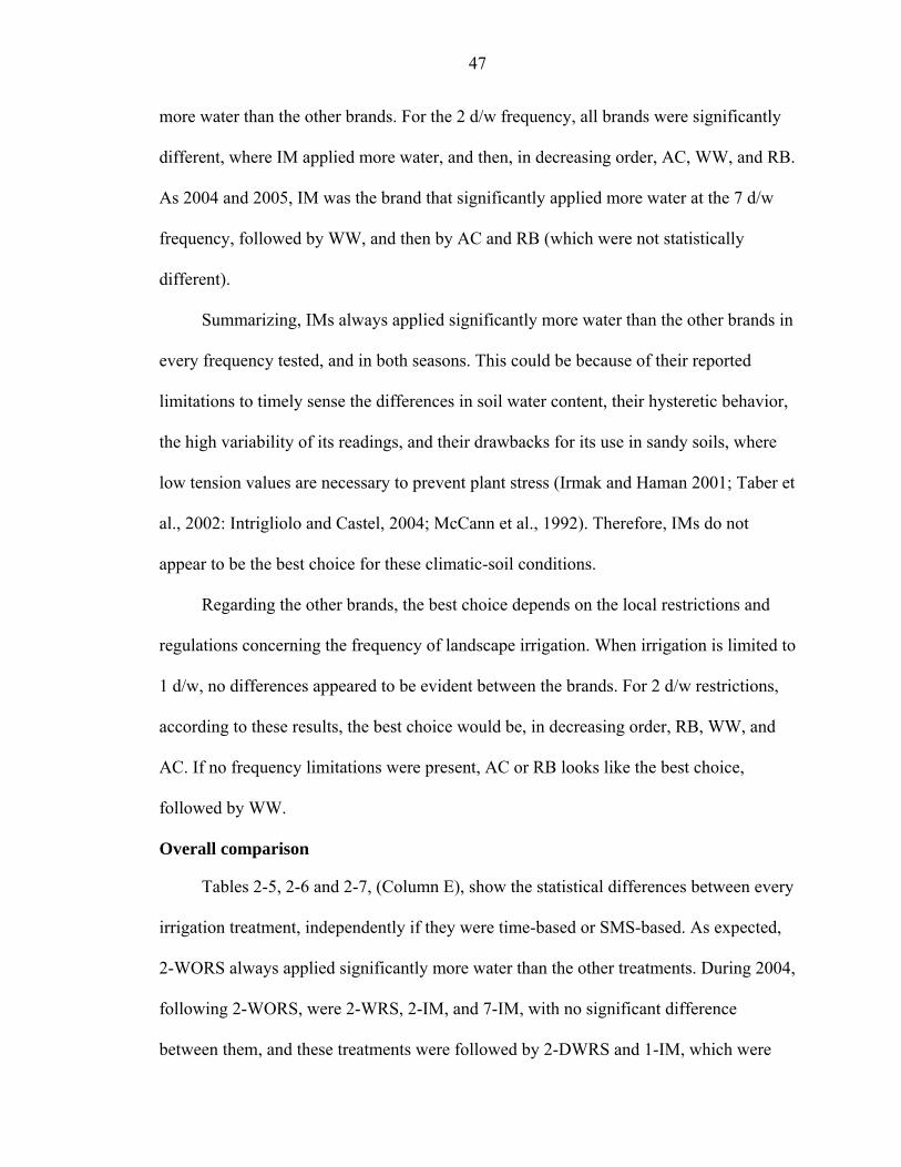
47
more water than the other brands. For the 2 d/w frequency, all brands were significantly
different, where IM applied more water, and then, in decreasing order, AC, WW, and RB.
As 2004 and 2005, IM was the brand that significantly applied more water at the 7 d/w
frequency, followed by WW, and then by AC and RB (which were not statistically
different).
Summarizing, IMs always applied significantly more water than the other brands in
every frequency tested, and in both seasons. This could be because of their reported
limitations to timely sense the differences in soil water content, their hysteretic behavior,
the high variability of its readings, and their drawbacks for its use in sandy soils, where
low tension values are necessary to prevent plant stress (Irmak and Haman 2001; Taber et
al., 2002: Intrigliolo and Castel, 2004; McCann et al., 1992). Therefore, IMs do not
appear to be the best choice for these climatic-soil conditions.
Regarding the other brands, the best choice depends on the local restrictions and
regulations concerning the frequency of landscape irrigation. When irrigation is limited to
1 d/w, no differences appeared to be evident between the brands. For 2 d/w restrictions,
according to these results, the best choice would be, in decreasing order, RB, WW, and
AC. If no frequency limitations were present, AC or RB looks like the best choice,
followed by WW.
Overall comparison
Tables 2-5, 2-6 and 2-7, (Column E), show the statistical differences between every
irrigation treatment, independently if they were time-based or SMS-based. As expected,
2-WORS always applied significantly more water than the other treatments. During 2004,
following 2-WORS, were 2-WRS, 2-IM, and 7-IM, with no significant difference
between them, and these treatments were followed by 2-DWRS and 1-IM, which were
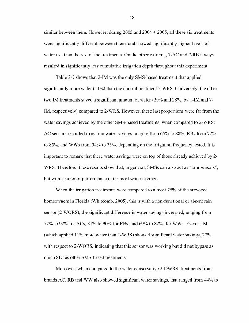
48
similar between them. However, during 2005 and 2004 + 2005, all these six treatments
were significantly different between them, and showed significantly higher levels of
water use than the rest of the treatments. On the other extreme, 7-AC and 7-RB always
resulted in significantly less cumulative irrigation depth throughout this experiment.
Table 2-7 shows that 2-IM was the only SMS-based treatment that applied
significantly more water (11%) than the control treatment 2-WRS. Conversely, the other
two IM treatments saved a significant amount of water (20% and 28%, by 1-IM and 7-
IM, respectively) compared to 2-WRS. However, these last proportions were far from the
water savings achieved by the other SMS-based treatments, when compared to 2-WRS:
AC sensors recorded irrigation water savings ranging from 65% to 88%, RBs from 72%
to 85%, and WWs from 54% to 73%, depending on the irrigation frequency tested. It is
important to remark that these water savings were on top of those already achieved by 2-
WRS. Therefore, these results show that, in general, SMSs can also act as “rain sensors”,
but with a superior performance in terms of water savings.
When the irrigation treatments were compared to almost 75% of the surveyed
homeowners in Florida (Whitcomb, 2005), this is with a non-functional or absent rain
sensor (2-WORS), the significant difference in water savings increased, ranging from
77% to 92% for ACs, 81% to 90% for RBs, and 69% to 82%, for WWs. Even 2-IM
(which applied 11% more water than 2-WRS) showed significant water savings, 27%
with respect to 2-WORS, indicating that this sensor was working but did not bypass as
much SIC as other SMS-based treatments.
Moreover, when compared to the water conservative 2-DWRS, treatments from
brands AC, RB and WW also showed significant water savings, that ranged from 44% to

49
80%, 55% to 76%, and 26 to 57%, respectively. On the other hand, all IM-frequencies
applied significantly more irrigation than 2-WORS, with values that ranged from 15% to
77% more water.
These results clearly demonstrate that the use of SMSs, along with traditional
timers in residential irrigation systems, could lead to important water savings. However,
the correct choice of the SMS, and its technology to measure or “sense” the soil water
status, is of great consequence.
Automation of Irrigation Systems
A complete automation of a residential irrigation system, based on SMSs, could be
achieved programming the timer to run every day as a scheduling strategy. Then, the
SMSs will allow the system to initiate the irrigation cycles only when it is actually
needed by the turfgrass, and override them when the sensed water content is over a pre-
set threshold.
In this experiment, this was confirmed when most of the SMS-based treatments
were able to follow the dry and rainy periods–controlling the amount of water to be
delivered to the different treatments (Table 2-4)–when the 7 d/w irrigation frequency
used significantly less water than the other frequencies (Table 2-7, Column C), and when
two of the SMS-based treatments programmed to run 7 d/w consistently used the smallest
amount of water (Tables 2-5, 2-6, and 2-7). In effect, treatments 7-AC and 7-RB recorded
total water savings of 85% or more, when compared to 2-WRS, and 90% or more when
compared to 2-WORS (Tables 2-7).
It is interesting to note that this concept (with a potential irrigation frequency of
seven days a week) is contradictory to the water use regulations and restrictions imposed
by the Water Management Districts and/or municipalities in Florida (where irrigation is

50
allowed only one or two days per week). However, these results suggest that choosing the
right type of sensor, and programming the automatic irrigation system to run everyday for
a short period of time (allowing the SMS to decide whether or not to irrigate), could save
large amounts of potable water used for irrigation purposes, and looks like a better BMP
than the current ones.
Moreover, this concept is not in opposition to the general recommendation for
deeper and less frequent irrigation for turfgrass, because these treatments (7-AC and 7-
RB) finally overrode more than 85% of the SIC (Table 2-4), resulting in a low actual
irrigation frequency, which was supplemented by large rainfall events.
Turfgrass Quality
No differences in turfgrass quality, including non-irrigated plots, were found
among treatments. This could be explained in part by the generally wet climatic
conditions that happened through almost all the time of the experiment, which favored
the growth and development of the bermudagrass. Another factor contributing to this,
even during the “dry” periods, could be found in the species itself. Common
bermudagrass is known as a more drought-tolerant grass compared to the pervasive St.
Augustinegrass [Stenotaphrum secundatum (Walt.) Kuntze] found in North-Central
Florida landscapes (Harivandi et al., 2001; Baldwin et al., 2005; Turgeon, 2005). As a
result, the treatment effects were buffered with respect of the turfgrass quality
parameters, and it could be concluded that no irrigation was necessary to maintain an
acceptable turf quality during the experiment time-period. Figure 2-37 shows, in Part A,
an homogeneous good quality between the different plots, and, in Part B, when
bermudagrass went dormant on all plots at the same time. Having analogous weather
conditions, Jordan et al. (2003) obtained similar results working with bentgrass.

51
Summary and Conclusions
High frequency rainfall events and a large amount of cumulative precipitation
prevailed during the time frame of this research, except for some weeks at the end of
2004 and at the early spring of 2005, when ETo exceeded rainfall. When the monthly
deficit rainfall values (relative to ETo) were correlated with the percent of irrigation
cycles allowed per month, r values of –0.93 and –0.76 were found for 2004 and 2005,
respectively. It was inferred that most of the SMS-based treatments automatically
canceled the majority of the irrigation cycles during the rainy periods, and responded to
dry periods by allowing irrigations to occur.
The three time-based treatments (2-WORS, 2-WRS, and 2-DWRS) were
significantly different from each other during the whole study period. The treatment
without a rain sensor (2-WORS) used, on average, 52% more water than the treatment
with a functional one (2-WRS), showing the importance of a well-maintained rain shut-
off device in all automated irrigation systems in Florida. On the other hand, treatment 2-
DWRS, applied close to 60% of the water applied by 2-WRS.
These time-based treatments were established to mimic the operation of irrigation
systems carried out by different homeowner profiles. However, according to the results of
this research, these treatments were fairly well managed compared to homeowners’ actual
operation practices in the Central Florida Ridge. Therefore, results in water use from this
experiment can be considered conservative and differences for actual homeowners could
be even larger.
When the time-based treatments were compared to the SMS-based treatments,
results showed that, on average, the SMS-based treatments were significantly more
efficient as a means to save water than the traditional time-based treatments. However,

52
not all SMS-treatments tested performed the same. The 2-IM treatment was the only
SMS-based treatment that applied significantly more water than the control 2-WRS (11%
more). The other two IM treatments, 1-IM and 7-IM, used significantly less water than 2-
WRS (20% and 28%, respectively), but always applied significantly more water than the
other brands/treatments in every frequency tested. Therefore, IMs do not appear to be the
best choice for the weather and soil conditions of this study.
All the other brands (AC, RB, and WW) recorded significant irrigation water
savings compared to the control 2-WRS, which ranged from 54% to 88%, depending on
the irrigation frequency. These results showed that most SMSs, except for 2-IM, can also
act as rain sensors, with superior performance in terms of water savings. When these last
brands were compared to 2-WORS, the differences in water savings increased, and
ranged from 69% to 92% over the 308-days study period.
Irrigation frequencies were also compared at the end of the study. All three
frequencies tested (1, 2, and 7 d/w) were significantly different. The 2 d/w frequency
used the highest volume of water, followed by the 1 d/w frequency, and 7 d/w was the
one that used the least amount of water. Moreover, and being part of this last frequency,
treatments 7-AC and 7-RB significantly and consistently used the smallest amount of
water regarding all treatments, during both seasons. They recorded total water savings of
85% or more, when compared to 2-WRS, and 90% or more when compared to 2-WORS.
These results suggest that scheduling low volume-high frequency irrigation cycles
(7 d/w) in Closed Control Loop irrigation systems, appears to be a better strategy
regarding water conservation for turfgrass irrigation in Florida’s sandy soils during rainy
periods, than scheduling irrigation cycles one or two days per week. Moreover, it was

53
concluded that no irrigation was necessary to maintain an acceptable turf quality during
the experimental period, which was evidenced by acceptable quality in non-irrigated
plots. Therefore, SMS-based technology could lead not only to a complete automation of
residential irrigation systems, but to save substantial irrigation water if implemented.
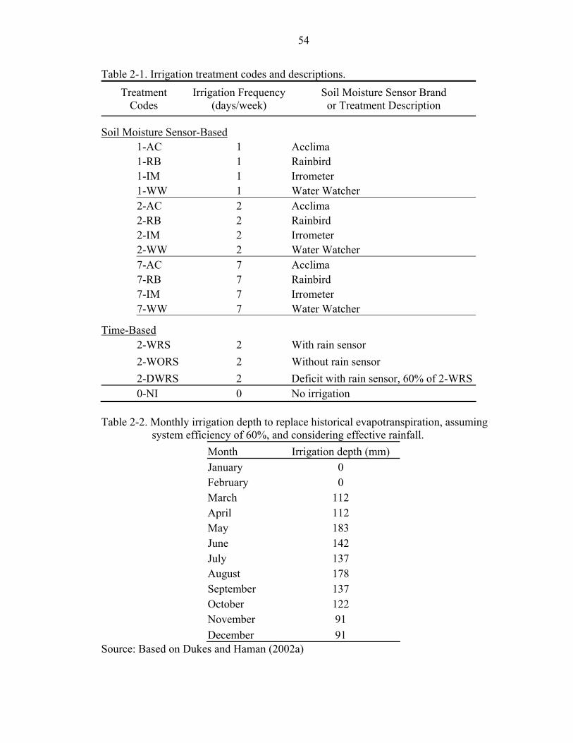
54
Table 2-1. Irrigation treatment codes and descriptions. Treatment
Codes Irrigation Frequency
(days/week) Soil Moisture Sensor Brand
or Treatment Description
Soil Moisture Sensor-Based 1-AC 1 Acclima 1-RB 1 Rainbird 1-IM 1 Irrometer 1-WW 1 Water Watcher 2-AC 2 Acclima 2-RB 2 Rainbird 2-IM 2 Irrometer 2-WW 2 Water Watcher 7-AC 7 Acclima 7-RB 7 Rainbird 7-IM 7 Irrometer 7-WW 7 Water Watcher
Time-Based 2-WRS 2 With rain sensor 2-WORS 2 Without rain sensor 2-DWRS 2 Deficit with rain sensor, 60% of 2-WRS 0-NI 0 No irrigation
Table 2-2. Monthly irrigation depth to replace historical evapotranspiration, assuming
system efficiency of 60%, and considering effective rainfall. Month Irrigation depth (mm) January 0 February 0 March 112 April 112 May 183 June 142 July 137 August 178 September 137 October 122 November 91 December 91
Source: Based on Dukes and Haman (2002a)
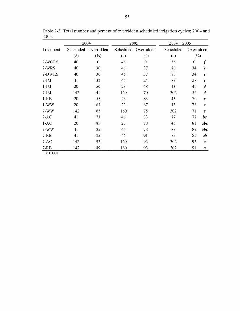
55
Table 2-3. Total number and percent of overridden scheduled irrigation cycles; 2004 and 2005. 2004 2005 2004 + 2005 Treatment Scheduled Overridden Scheduled Overridden Scheduled Overridden (#) (%) (#) (%) (#) (%) 2-WORS 40 0 46 0 86 0 f 2-WRS 40 30 46 37 86 34 e 2-DWRS 40 30 46 37 86 34 e 2-IM 41 32 46 24 87 28 e 1-IM 20 50 23 48 43 49 d 7-IM 142 41 160 70 302 56 d 1-RB 20 55 23 83 43 70 c 1-WW 20 63 23 87 43 76 c 7-WW 142 65 160 75 302 71 c 2-AC 41 73 46 83 87 78 bc1-AC 20 85 23 78 43 81 abc2-WW 41 85 46 78 87 82 abc2-RB 41 85 46 91 87 89 ab7-AC 142 92 160 92 302 92 a 7-RB 142 89 160 93 302 91 a P<0.0001
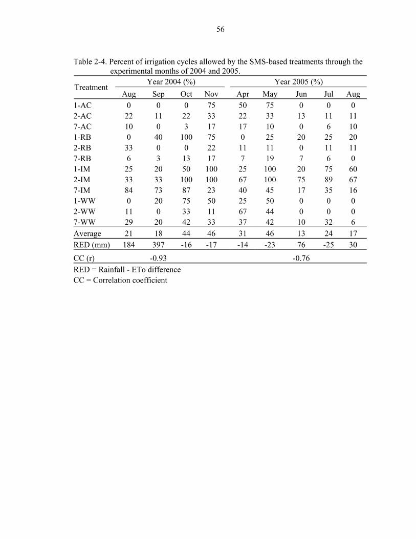
56
Table 2-4. Percent of irrigation cycles allowed by the SMS-based treatments through the
experimental months of 2004 and 2005. Year 2004 (%) Year 2005 (%)
Treatment Aug Sep Oct Nov Apr May Jun Jul Aug
1-AC 0 0 0 75 50 75 0 0 0 2-AC 22 11 22 33 22 33 13 11 11 7-AC 10 0 3 17 17 10 0 6 10 1-RB 0 40 100 75 0 25 20 25 20 2-RB 33 0 0 22 11 11 0 11 11 7-RB 6 3 13 17 7 19 7 6 0 1-IM 25 20 50 100 25 100 20 75 60 2-IM 33 33 100 100 67 100 75 89 67 7-IM 84 73 87 23 40 45 17 35 16 1-WW 0 20 75 50 25 50 0 0 0 2-WW 11 0 33 11 67 44 0 0 0 7-WW 29 20 42 33 37 42 10 32 6 Average 21 18 44 46 31 46 13 24 17 RED (mm) 184 397 -16 -17 -14 -23 76 -25 30 CC (r) -0.93 -0.76 RED = Rainfall - ETo difference CC = Correlation coefficient
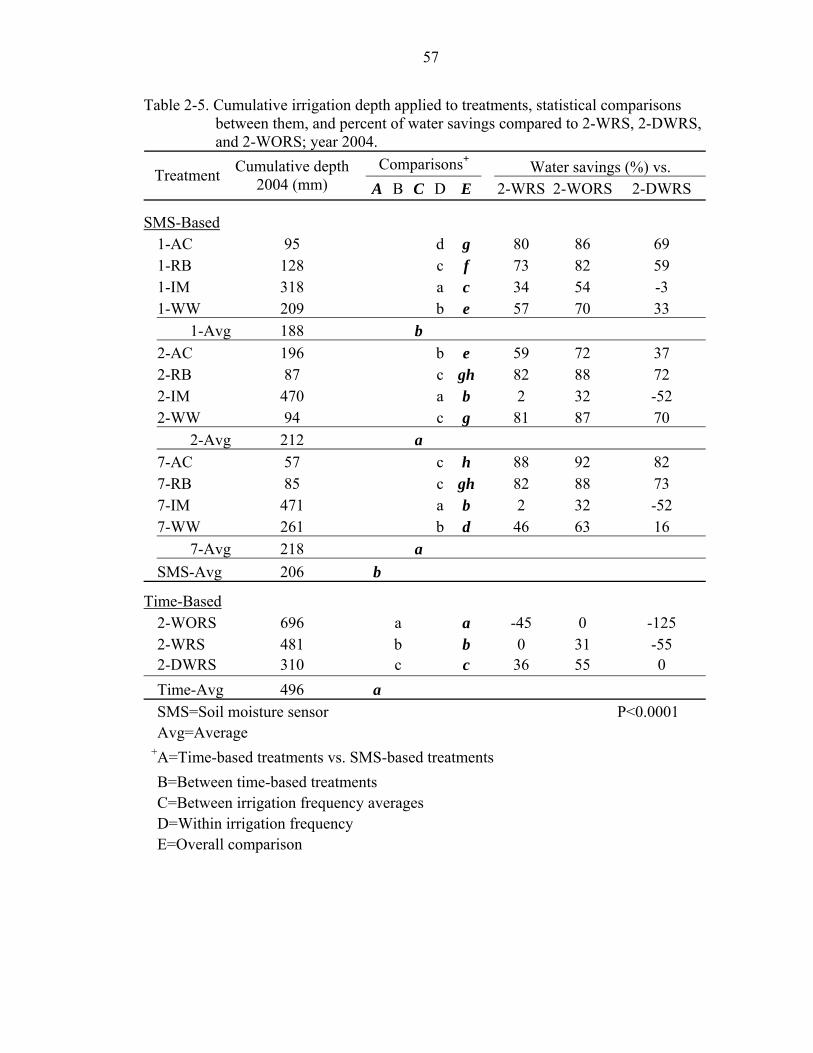
57
Table 2-5. Cumulative irrigation depth applied to treatments, statistical comparisons between them, and percent of water savings compared to 2-WRS, 2-DWRS, and 2-WORS; year 2004.
Comparisons+ Water savings (%) vs. Treatment Cumulative depth 2004 (mm) A B C D E 2-WRS 2-WORS 2-DWRS
SMS-Based 1-AC 95 d g 80 86 69 1-RB 128 c f 73 82 59 1-IM 318 a c 34 54 -3 1-WW 209 b e 57 70 33 1-Avg 188 b 2-AC 196 b e 59 72 37 2-RB 87 c gh 82 88 72 2-IM 470 a b 2 32 -52 2-WW 94 c g 81 87 70 2-Avg 212 a 7-AC 57 c h 88 92 82 7-RB 85 c gh 82 88 73 7-IM 471 a b 2 32 -52 7-WW 261 b d 46 63 16 7-Avg 218 a SMS-Avg 206 b
Time-Based 2-WORS 696 a a -45 0 -125 2-WRS 481 b b 0 31 -55 2-DWRS 310 c c 36 55 0 Time-Avg 496 a
SMS=Soil moisture sensor P<0.0001 Avg=Average
+A=Time-based treatments vs. SMS-based treatments B=Between time-based treatments
C=Between irrigation frequency averages D=Within irrigation frequency E=Overall comparison

58
Table 2-6. Cumulative irrigation depth applied to treatments, statistical comparisons between them, and percent of water savings compared to 2-WRS, 2-DWRS, and 2-WORS; year 2005.
Comparisons+ Water savings (%) vs. Treatment Cumulative depth 2005 (mm) A B C D E 2-WRS 2-WORS 2-DWRS
SMS-Based 1-AC 188 b gh 63 77 40 1-RB 153 c i 70 81 51 1-IM 475 a d 7 42 -52 1-WW 114 d j 78 86 64 1-Avg 232 b 2-AC 152 b i 70 81 51 2-RB 101 c j 80 88 68 2-IM 635 a b -24 22 -103 2-WW 177 b h 66 78 44 2-Avg 266 a 7-AC 65 c k 87 92 79 7-RB 62 c k 88 92 80 7-IM 244 a f 52 70 22 7-WW 202 b g 61 75 36 7-Avg 143 c SMS-Avg 214 b
Time-Based 2-WORS 818 a a -59 0 -161 2-WRS 514 b c 0 37 -64 2-DWRS 313 c e 39 62 0 Time-Avg 548 a
SMS=Soil moisture sensor P<0.0001 Avg=Average
+A=Time-based treatments vs. SMS-based treatments B=Between time-based treatments
C=Between irrigation frequency averages D=Within irrigation frequency E=Overall comparison
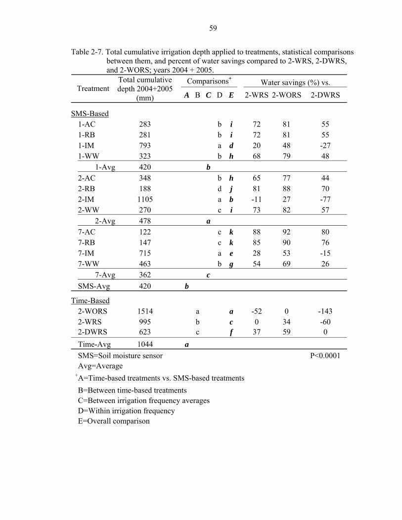
59
Table 2-7. Total cumulative irrigation depth applied to treatments, statistical comparisons between them, and percent of water savings compared to 2-WRS, 2-DWRS, and 2-WORS; years 2004 + 2005.
Comparisons+ Water savings (%) vs. Treatment
Total cumulative depth 2004+2005
(mm) A B C D E 2-WRS 2-WORS 2-DWRS
SMS-Based 1-AC 283 b i 72 81 55 1-RB 281 b i 72 81 55 1-IM 793 a d 20 48 -27 1-WW 323 b h 68 79 48 1-Avg 420 b 2-AC 348 b h 65 77 44 2-RB 188 d j 81 88 70 2-IM 1105 a b -11 27 -77 2-WW 270 c i 73 82 57 2-Avg 478 a 7-AC 122 c k 88 92 80 7-RB 147 c k 85 90 76 7-IM 715 a e 28 53 -15 7-WW 463 b g 54 69 26 7-Avg 362 c SMS-Avg 420 b
Time-Based 2-WORS 1514 a a -52 0 -143 2-WRS 995 b c 0 34 -60 2-DWRS 623 c f 37 59 0 Time-Avg 1044 a
SMS=Soil moisture sensor P<0.0001 Avg=Average
+A=Time-based treatments vs. SMS-based treatments B=Between time-based treatments
C=Between irrigation frequency averages D=Within irrigation frequency E=Overall comparison
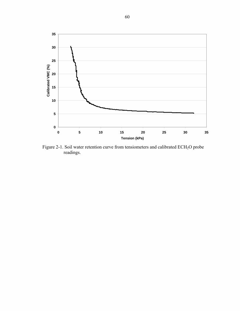
60
0
5
10
15
20
25
30
35
0 5 10 15 20 25 30 35Tension (kPa)
Cal
ibra
ted
VMC
(%)
Figure 2-1. Soil water retention curve from tensiometers and calibrated ECH2O probe
readings.
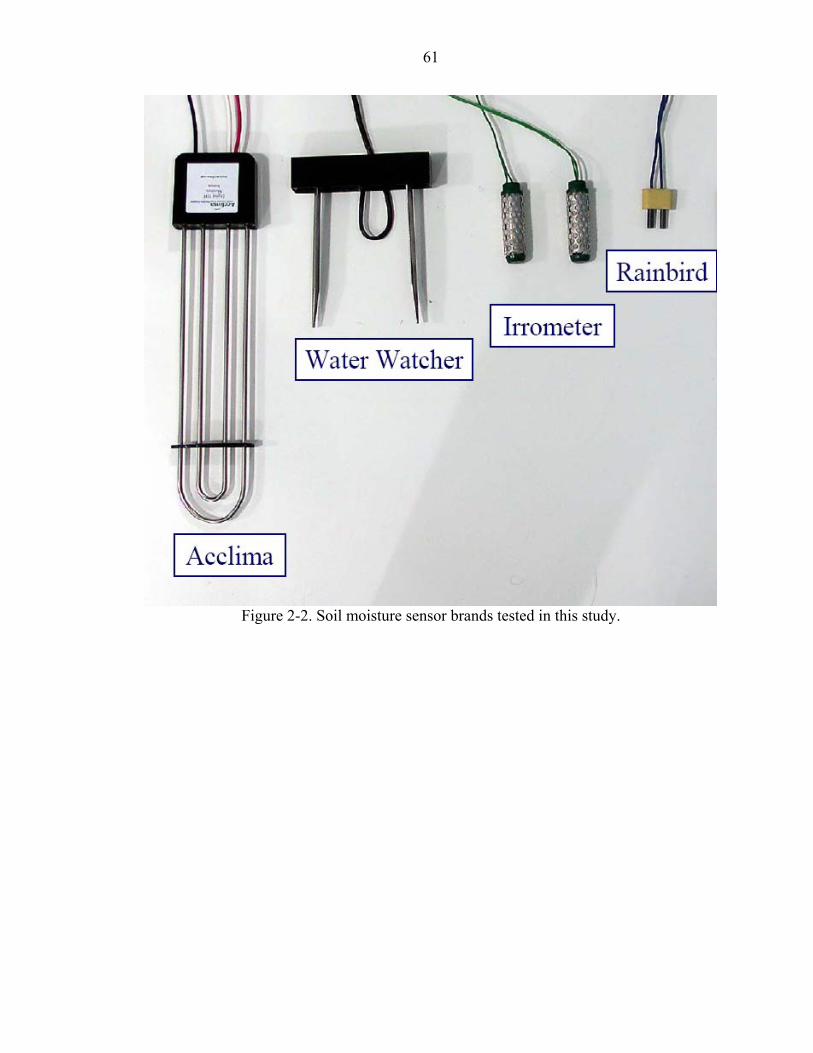
61
Figure 2-2. Soil moisture sensor brands tested in this study.
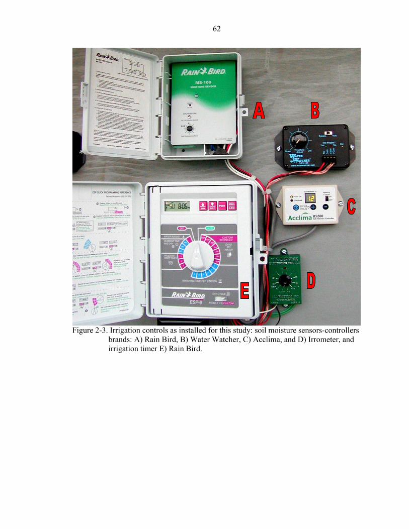
62
Figure 2-3. Irrigation controls as installed for this study: soil moisture sensors-controllers
brands: A) Rain Bird, B) Water Watcher, C) Acclima, and D) Irrometer, and irrigation timer E) Rain Bird.
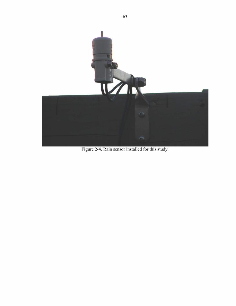
63
Figure 2-4. Rain sensor installed for this study.
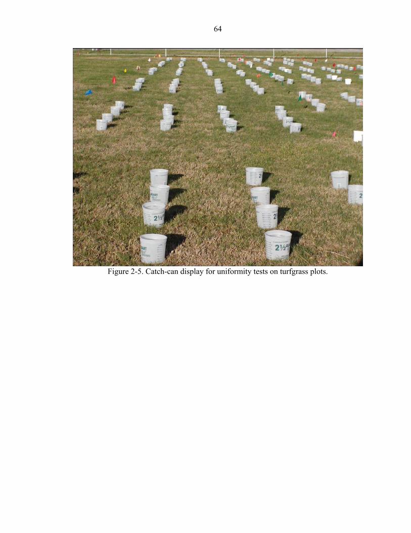
64
Figure 2-5. Catch-can display for uniformity tests on turfgrass plots.
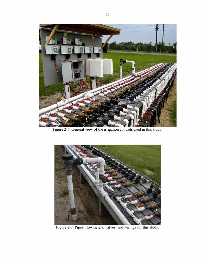
65
Figure 2-6. General view of the irrigation controls used in this study.
Figure 2-7. Pipes, flowmeters, valves, and wirings for this study.
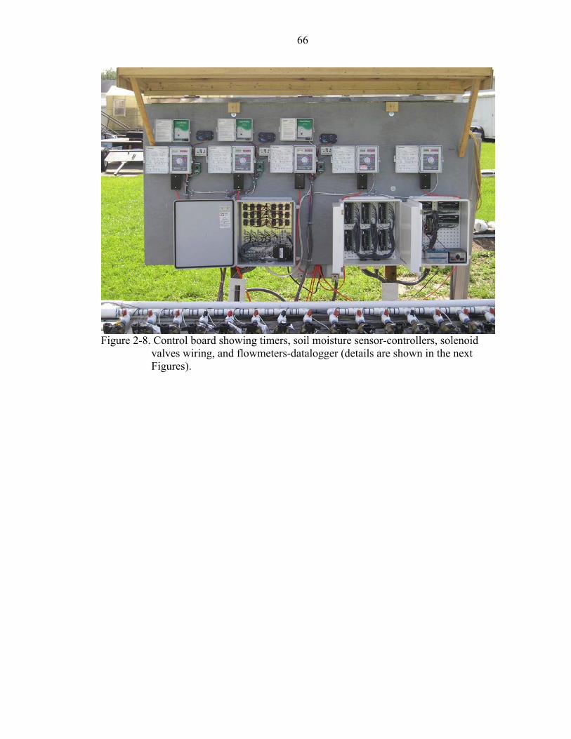
66
Figure 2-8. Control board showing timers, soil moisture sensor-controllers, solenoid
valves wiring, and flowmeters-datalogger (details are shown in the next Figures).
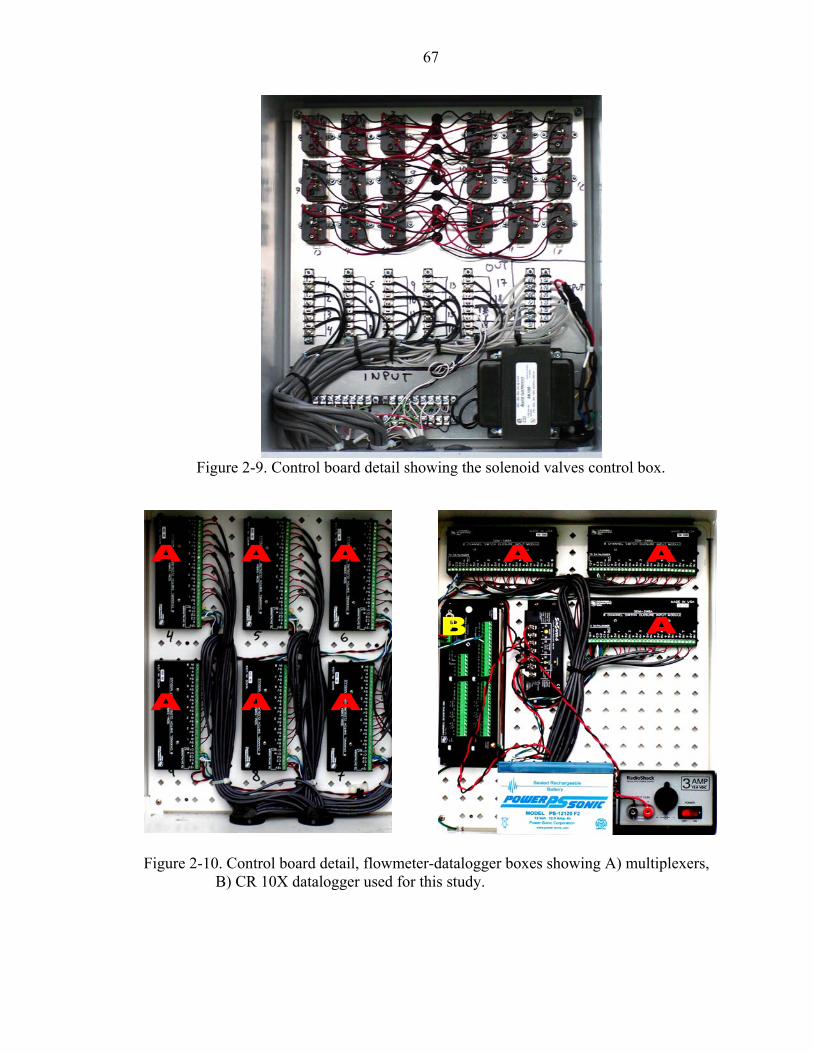
67
Figure 2-9. Control board detail showing the solenoid valves control box.
Figure 2-10. Control board detail, flowmeter-datalogger boxes showing A) multiplexers,
B) CR 10X datalogger used for this study.

68
Figure 2-11. Automated weather station near turf plots for this study.
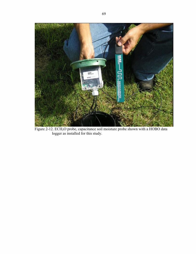
69
Figure 2-12. ECH2O probe, capacitance soil moisture probe shown with a HOBO data
logger as installed for this study.
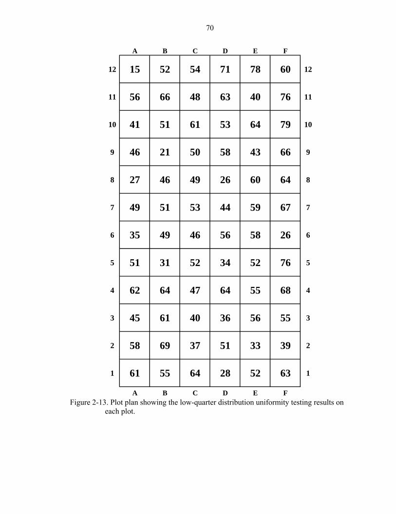
70
A B C D E F
12 15 52 54 71 78 60 12
11 56 66 48 63 40 76 11
10 41 51 61 53 64 79 10
9 46 21 50 58 43 66 9
8 27 46 49 26 60 64 8
7 49 51 53 44 59 67 7
6 35 49 46 56 58 26 6
5 51 31 52 34 52 76 5
4 62 64 47 64 55 68 4
3 45 61 40 36 56 55 3
2 58 69 37 51 33 39 2
1 61 55 64 28 52 63 1
A B C D E F Figure 2-13. Plot plan showing the low-quarter distribution uniformity testing results on
each plot.

71
A B C D E F
12 15.2 6.4 7.4 8.8 5.6 4.4 12
11 14.0 5.4 5.4 11.4 6.8 4.0 11
10 6.4 6.2 6.8 10.2 6.0 7.0 10
9 6.0 6.0 7.4 10.0 8.0 7.6 9
8 4.6 5.6 9.6 7.8 9.4 8.4 8
7 4.4 5.6 6.4 7.8 9.2 9.0 7
6 5.4 4.6 6.6 9.4 8.0 5.8 6
5 3.6 7.4 5.8 9.2 7.6 5.2 5
4 4.4 5.0 5.6 7.8 8.4 6.4 4
3 5.8 6.0 6.0 7.4 7.2 5.6 3
2 5.8 5.6 6.2 6.8 6.6 5.8 2
1 4.4 7.2 6.0 6.6 8.2 8.4 1
A B C D E F Figure 2-14. Plot plan showing average volumetric water content (%) on each plot during
a relatively “dry” period. Plots in red were discarded, and plots in green were used for placement of SMSs.

72
A B C D E F
12 20.8 11.0 11.6 12.2 11.0 12.4 12
11 27.8 11.6 12.2 12.8 10.8 9.4 11
10 12.4 8.8 10.4 10.4 10.8 9.8 10
9 11.4 11.2 11.0 11.4 10.4 10.8 9
8 11.4 10.6 12.6 12.2 11.8 10.6 8
7 10.2 9.6 12.0 11.0 11.0 11.2 7
6 10.6 11.6 10.2 10.8 9.6 9.2 6
5 9.2 12.2 10.4 9.6 10.4 9.8 5
4 9.8 10.2 9.8 9.4 8.8 9.2 4
3 9.8 9.8 12.0 10.4 10.8 8.6 3
2 12.0 11.2 10.2 11.2 14.0 10.6 2
1 12.2 11.6 11.2 12.0 14.8 15.8 1
A B C D E F Figure 2-15. Plot plan showing average volumetric water content (%) on each plot during
a relatively “wet” condition. Plots in red were discarded, and plots in green were used for placement of SMSs.
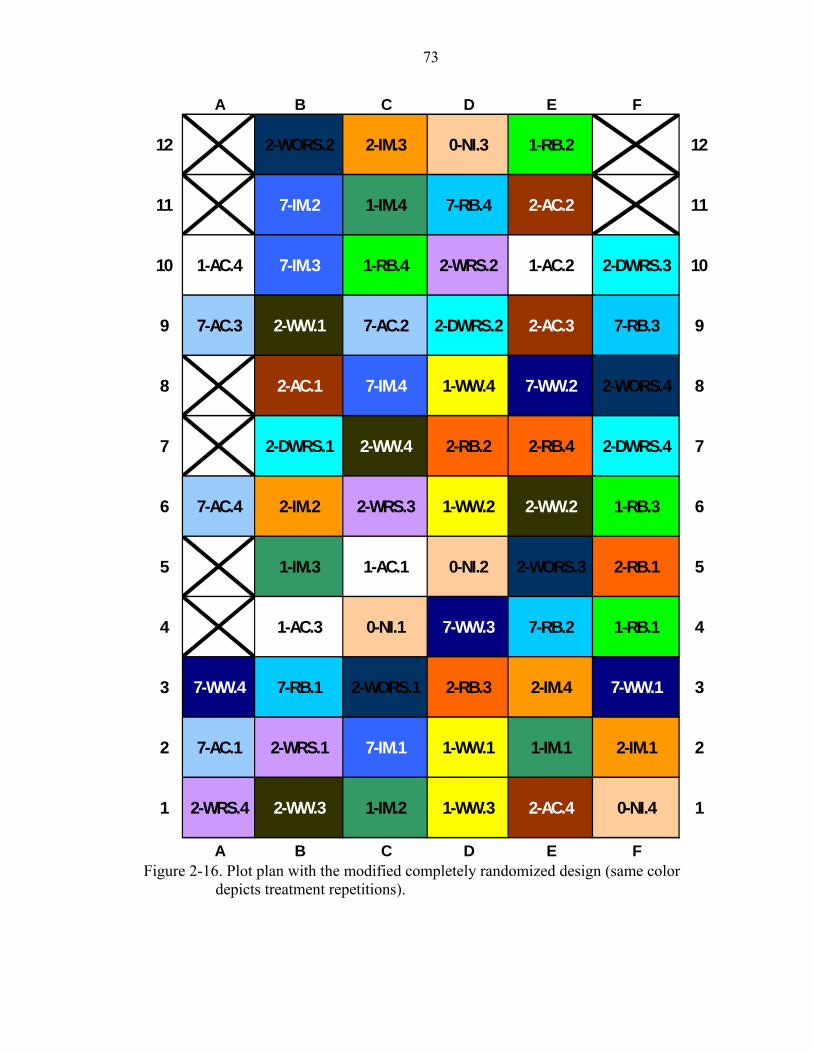
73
A B C D E F
12 2-WORS.2 2-IM.3 0-NI.3 1-RB.2 12
11 7-IM.2 1-IM.4 7-RB.4 2-AC.2 11
10 1-AC.4 7-IM.3 1-RB.4 2-WRS.2 1-AC.2 2-DWRS.3 10
9 7-AC.3 2-WW.1 7-AC.2 2-DWRS.2 2-AC.3 7-RB.3 9
8 2-AC.1 7-IM.4 1-WW.4 7-WW.2 2-WORS.4 8
7 2-DWRS.1 2-WW.4 2-RB.2 2-RB.4 2-DWRS.4 7
6 7-AC.4 2-IM.2 2-WRS.3 1-WW.2 2-WW.2 1-RB.3 6
5 1-IM.3 1-AC.1 0-NI.2 2-WORS.3 2-RB.1 5
4 1-AC.3 0-NI.1 7-WW.3 7-RB.2 1-RB.1 4
3 7-WW.4 7-RB.1 2-WORS.1 2-RB.3 2-IM.4 7-WW.1 3
2 7-AC.1 2-WRS.1 7-IM.1 1-WW.1 1-IM.1 2-IM.1 2
1 2-WRS.4 2-WW.3 1-IM.2 1-WW.3 2-AC.4 0-NI.4 1
A B C D E F Figure 2-16. Plot plan with the modified completely randomized design (same color
depicts treatment repetitions).
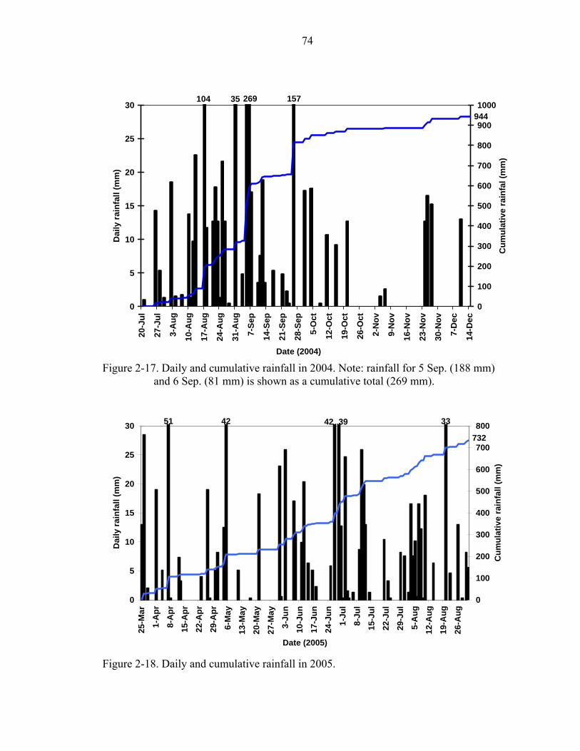
74
157269104 35
944
0
5
10
15
20
25
30
20-J
ul
27-J
ul
3-A
ug
10-A
ug
17-A
ug
24-A
ug
31-A
ug
7-Se
p
14-S
ep
21-S
ep
28-S
ep
5-O
ct
12-O
ct
19-O
ct
26-O
ct
2-N
ov
9-N
ov
16-N
ov
23-N
ov
30-N
ov
7-D
ec
14-D
ec
Date (2004)
Dai
ly ra
infa
ll (m
m)
0
100
200
300
400
500
600
700
800
900
1000
Cum
ulat
ive
rain
fal (
mm
)
Figure 2-17. Daily and cumulative rainfall in 2004. Note: rainfall for 5 Sep. (188 mm)
and 6 Sep. (81 mm) is shown as a cumulative total (269 mm).
3942 334251
732
0
5
10
15
20
25
30
25-M
ar
1-A
pr8-
Apr
15-A
pr22
-Apr
29-A
pr6-
May
13-M
ay20
-May
27-M
ay3-
Jun
10-J
un17
-Jun
24-J
un1-
Jul
8-Ju
l15
-Jul
22-J
ul29
-Jul
5-A
ug12
-Aug
19-A
ug
26-A
ug
Date (2005)
Dai
ly ra
infa
ll (m
m)
0
100
200
300
400
500
600
700
800
Cum
ulat
ive
rain
fall
(mm
)
Figure 2-18. Daily and cumulative rainfall in 2005.
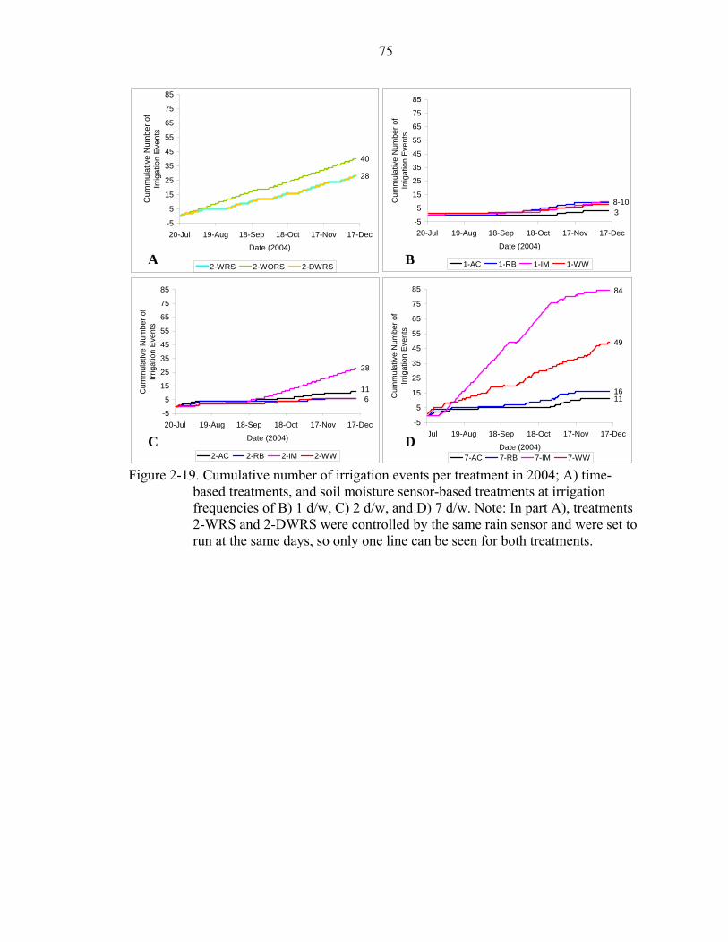
75
40
28
-5
5
15
25
35
45
55
65
75
85
20-Jul 19-Aug 18-Sep 18-Oct 17-Nov 17-DecDate (2004)
Cum
mul
ativ
e N
umbe
r of
Irrig
atio
n Ev
ents
2-WRS 2-WORS 2-DWRS
38-10
-5
5
15
25
35
45
55
65
75
85
20-Jul 19-Aug 18-Sep 18-Oct 17-Nov 17-Dec
Date (2004)
Cum
mul
ativ
e N
umbe
r of
Irrig
atio
n E
vent
s
1-AC 1-RB 1-IM 1-WW
11
28
6
-5
5
15
25
35
45
55
65
75
85
20-Jul 19-Aug 18-Sep 18-Oct 17-Nov 17-Dec
Date (2004)
Cum
mul
ativ
e N
umbe
r of
Irrig
atio
n E
vent
s
2-AC 2-RB 2-IM 2-WW
1116
84
49
-5
5
15
25
35
45
55
65
75
85
20-Jul 19-Aug 18-Sep 18-Oct 17-Nov 17-Dec
Date (2004)
Cum
mul
ativ
e N
umbe
r of
Irrig
atio
n E
vent
s
7-AC 7-RB 7-IM 7-WW Figure 2-19. Cumulative number of irrigation events per treatment in 2004; A) time-
based treatments, and soil moisture sensor-based treatments at irrigation frequencies of B) 1 d/w, C) 2 d/w, and D) 7 d/w. Note: In part A), treatments 2-WRS and 2-DWRS were controlled by the same rain sensor and were set to run at the same days, so only one line can be seen for both treatments.
A B
C D
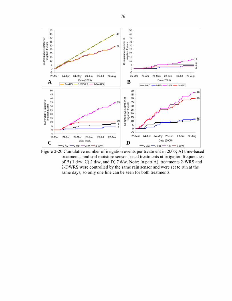
76
54
12
3
-505
101520253035404550
25-Mar 24-Apr 24-May 23-Jun 23-Jul 22-Aug
Date (2005)
Cum
mul
ativ
e N
umbe
r of
Irrig
atio
n E
vent
s
1-AC 1-RB 1-IM 1-WW
84
35
10
-5
0
5
1015
20
25
30
35
40
45
50
25-Mar 24-Apr 24-May 23-Jun 23-Jul 22-Aug
Date (2005)
Cum
mul
ativ
e N
umbe
r of
Irrig
atio
n E
vent
s
2-AC 2-RB 2-IM 2-WW
1312
48
40
-505
101520253035404550
25-Mar 24-Apr 24-May 23-Jun 23-Jul 22-AugDate (2005)
Cum
mul
ativ
e N
umbe
r of
Irrig
atio
n Ev
ents
7-AC 7-RB 7-IM 7-WW
45
29
-505
101520253035404550
25-Mar 24-Apr 24-May 23-Jun 23-Jul 22-AugDate (2005)
Cum
mul
ativ
e N
umbe
r of
Irrig
atio
n E
vent
s
2-WRS 2-WORS 2-DWRS
Figure 2-20 Cumulative number of irrigation events per treatment in 2005; A) time-based
treatments, and soil moisture sensor-based treatments at irrigation frequencies of B) 1 d/w, C) 2 d/w, and D) 7 d/w. Note: In part A), treatments 2-WRS and 2-DWRS were controlled by the same rain sensor and were set to run at the same days, so only one line can be seen for both treatments.
D C
A B
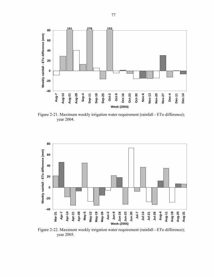
77
153276101
-40
-20
0
20
40
60
80
Aug
-7
Aug
-14
Aug
-21
Aug
-28
Sep-
4
Sep-
11
Sep-
18
Sep-
25
Oct
-2
Oct
-9
Oct
-16
Oct
-23
Oct
-30
Nov
-6
Nov
-13
Nov
-20
Nov
-27
Dec
-4
Dec
-11
Dec
-14
Week (2004)
Wee
kly
rain
fall
- ETo
diff
eren
ce (m
m)
Figure 2-21. Maximum weekly irrigation water requirement (rainfall - ETo difference);
year 2004.
-40
-20
0
20
40
60
80
Mar
-31
Apr
-7
Apr
-14
Apr
-21
Apr
-28
May
-5
May
-12
May
-19
May
-26
Jun-
2
Jun-
9
Jun-
16
Jun-
23
Jun-
30
Jul-7
Jul-1
4
Jul-2
1
Jul-2
8
Aug
-4
Aug
-11
Aug
-18
Aug
-25
Aug
-31
Week (2005)
Wee
kly
rain
fall
- ETo
diff
eren
ce (m
m)
Figure 2-22. Maximum weekly irrigation water requirement (rainfall - ETo difference);
year 2005.

78
Figure 2-23. Volumetric moisture content through time, on treatment 0-NI, year 2004.

79
Figure 2-24. Volumetric moisture content (VMC) through time, showing results of the scheduled irrigation cycles (SIC), where the
blue dots represent bypassed SIC, the red dots represent allowed SIC, and the red lines represent the range of VMC when the SIC were allowed; treatment 1-AC, year 2004.
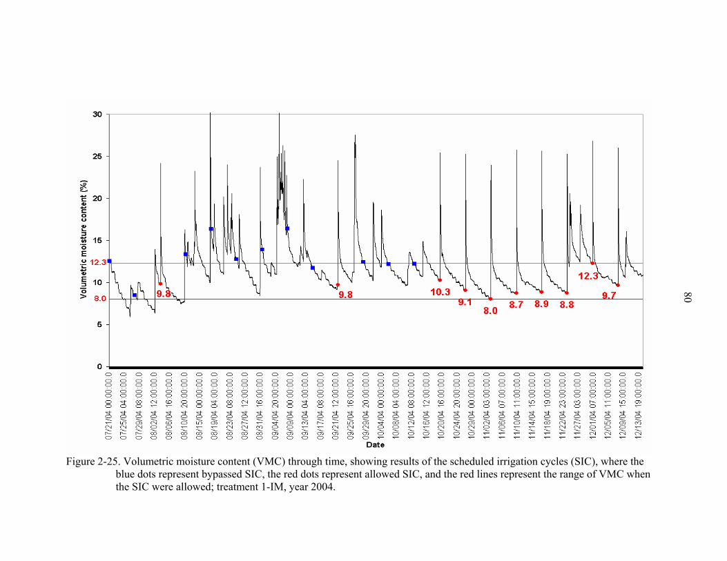
80
Figure 2-25. Volumetric moisture content (VMC) through time, showing results of the scheduled irrigation cycles (SIC), where the
blue dots represent bypassed SIC, the red dots represent allowed SIC, and the red lines represent the range of VMC when the SIC were allowed; treatment 1-IM, year 2004.
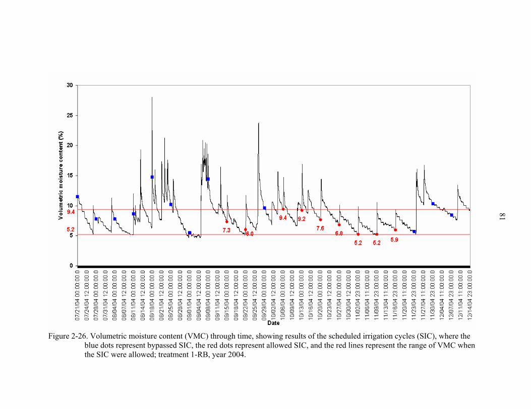
81
Figure 2-26. Volumetric moisture content (VMC) through time, showing results of the scheduled irrigation cycles (SIC), where the
blue dots represent bypassed SIC, the red dots represent allowed SIC, and the red lines represent the range of VMC when the SIC were allowed; treatment 1-RB, year 2004.
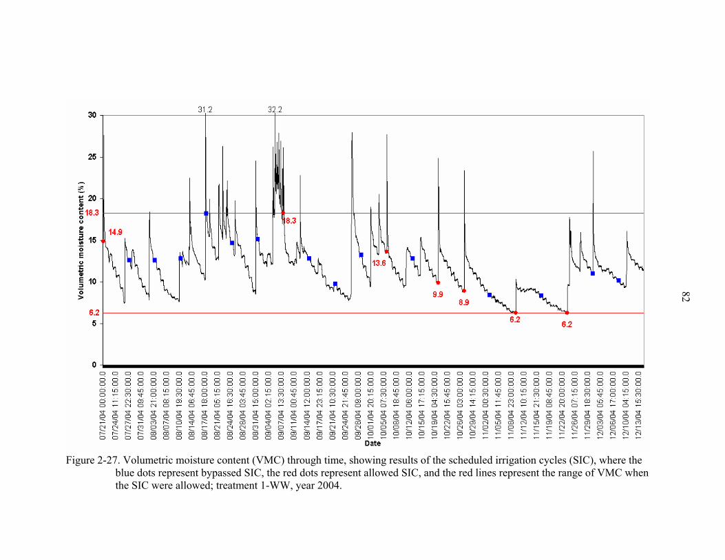
82
Figure 2-27. Volumetric moisture content (VMC) through time, showing results of the scheduled irrigation cycles (SIC), where the
blue dots represent bypassed SIC, the red dots represent allowed SIC, and the red lines represent the range of VMC when the SIC were allowed; treatment 1-WW, year 2004.

83
Figure 2-28. Volumetric moisture content (VMC) through time, showing results of the scheduled irrigation cycles (SIC), where the
blue dots represent bypassed SIC, the red dots represent allowed SIC, and the red lines represent the range of VMC when the SIC were allowed; treatment 2-AC, year 2004.
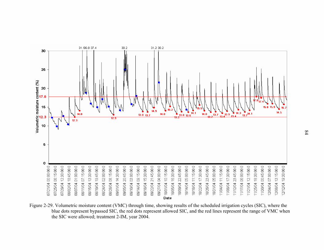
84
Figure 2-29. Volumetric moisture content (VMC) through time, showing results of the scheduled irrigation cycles (SIC), where the
blue dots represent bypassed SIC, the red dots represent allowed SIC, and the red lines represent the range of VMC when the SIC were allowed; treatment 2-IM, year 2004.
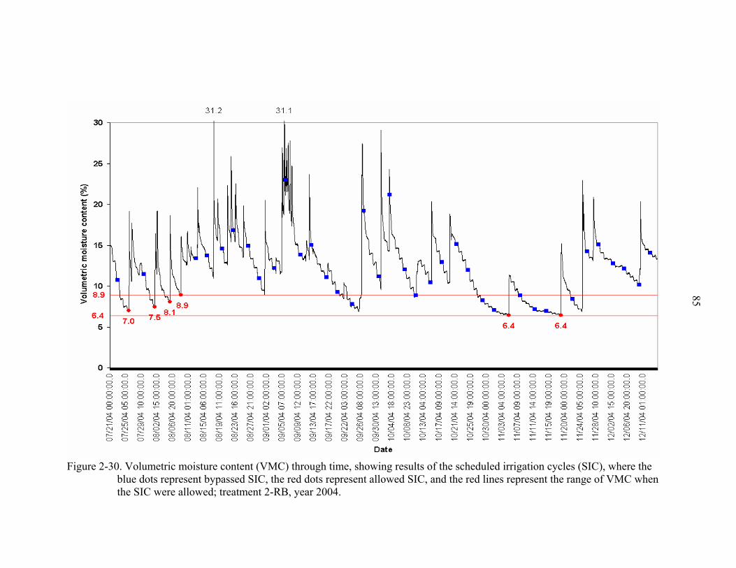
85
Figure 2-30. Volumetric moisture content (VMC) through time, showing results of the scheduled irrigation cycles (SIC), where the
blue dots represent bypassed SIC, the red dots represent allowed SIC, and the red lines represent the range of VMC when the SIC were allowed; treatment 2-RB, year 2004.

86
Figure 2-31. Volumetric moisture content (VMC) through time, showing results of the scheduled irrigation cycles (SIC), where the
blue dots represent bypassed SIC, the red dots represent allowed SIC, and the red lines represent the range of VMC when the SIC were allowed; treatment 2-WW, year 2004.
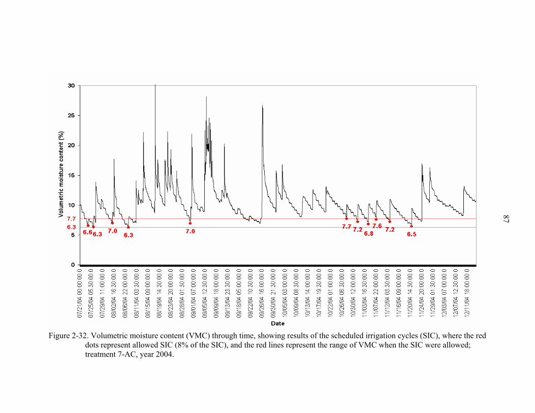
87
Figure 2-32. Volumetric moisture content (VMC) through time, showing results of the scheduled irrigation cycles (SIC), where the red
dots represent allowed SIC (8% of the SIC), and the red lines represent the range of VMC when the SIC were allowed; treatment 7-AC, year 2004.
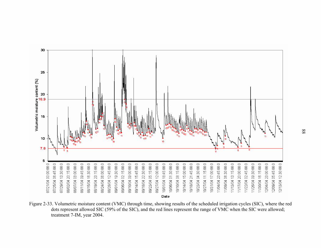
88
Figure 2-33. Volumetric moisture content (VMC) through time, showing results of the scheduled irrigation cycles (SIC), where the red
dots represent allowed SIC (59% of the SIC), and the red lines represent the range of VMC when the SIC were allowed; treatment 7-IM, year 2004.
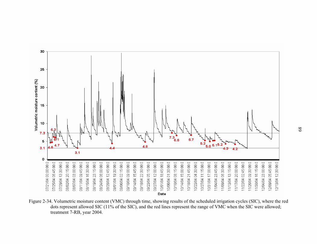
89
Figure 2-34. Volumetric moisture content (VMC) through time, showing results of the scheduled irrigation cycles (SIC), where the red
dots represent allowed SIC (11% of the SIC), and the red lines represent the range of VMC when the SIC were allowed; treatment 7-RB, year 2004.

90
Figure 2-35. Volumetric moisture content (VMC) through time, showing results of the scheduled irrigation cycles (SIC), where the red
dots represent allowed SIC (35% of the SIC), and the red lines represent the range of VMC when the SIC were allowed; treatment 7-WW, year 2004.
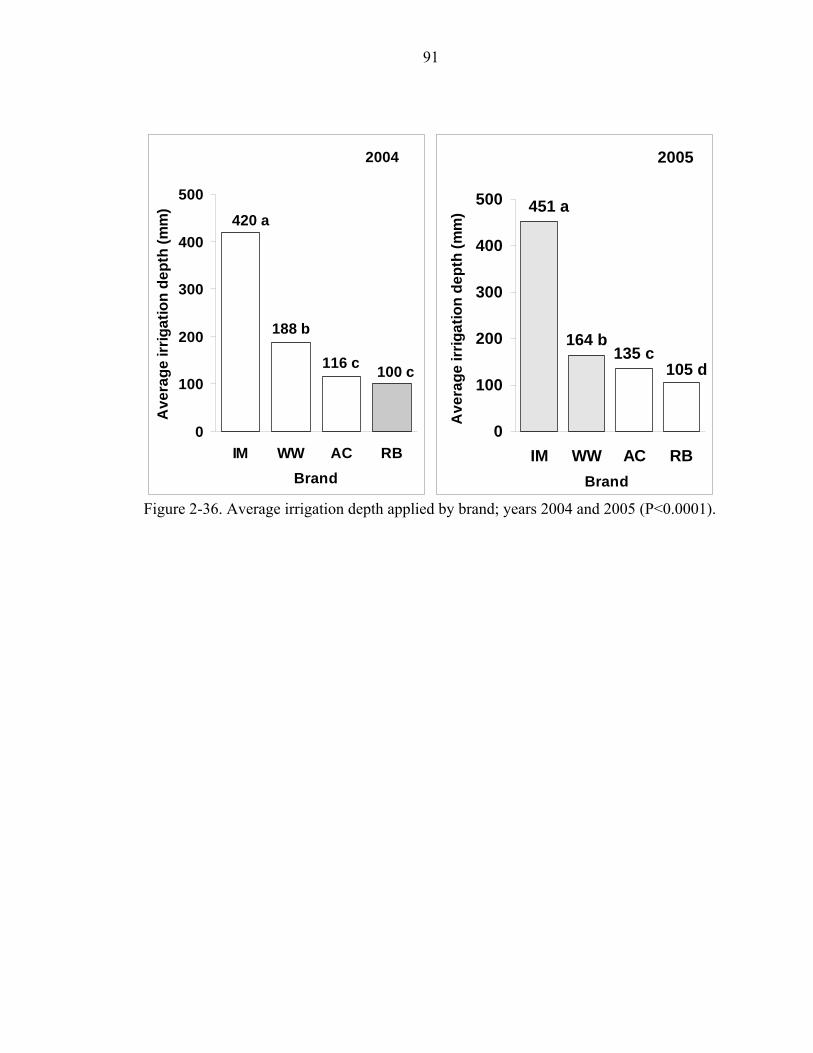
91
2004
100 c116 c
188 b
420 a
0
100
200
300
400
500
IM WW AC RBBrand
Ave
rage
irrig
atio
n de
pth
(mm
)2005
105 d135 c
164 b
451 a
0
100
200
300
400
500
IM WW AC RBBrand
Ave
rage
irrig
atio
n de
pth
(mm
)
Figure 2-36. Average irrigation depth applied by brand; years 2004 and 2005 (P<0.0001).
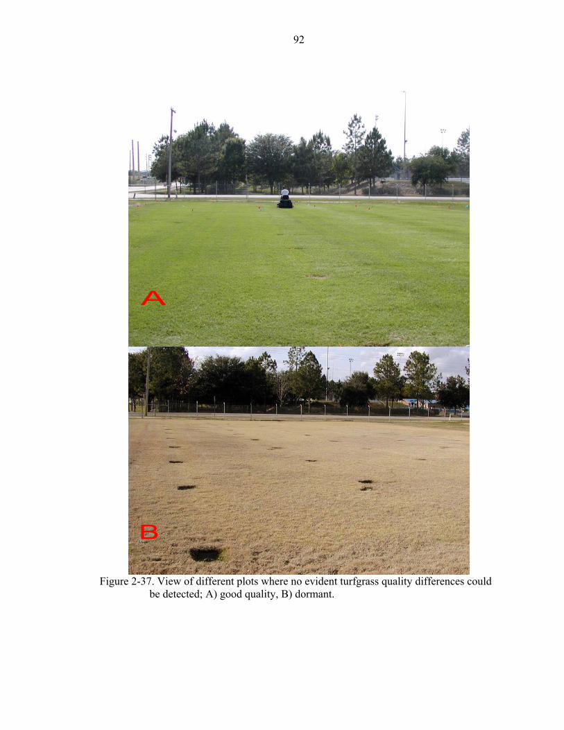
92
Figure 2-37. View of different plots where no evident turfgrass quality differences could
be detected; A) good quality, B) dormant.

93
CHAPTER 3 EXPANDING DISK RAIN SENSOR PERFORMANCE AND POTENTIAL
IRRIGATION WATER SAVINGS
Rain Sensors
A rain sensor (RS), also called rain shut-off device or rain switch (Figures 3-1 and
3-2), is a device designed to interrupt a scheduled cycle of an automatic irrigation system
controller (i.e. timer), when a specific amount of rainfall has occurred (Dukes and
Haman, 2002b; Hunter Industries, Inc., 2006).
Rain shut-off devices are the most common type of irrigation-sensor, due to an
increasing number of municipalities throughout the country that have mandates and/or
cost-saving programs for their use, on new and existing residential and commercial
irrigation systems. In addition, and except for the most arid environments, they appear to
be a useful tool for water conservation, at a relatively low cost (Dewey, 2003).
Currently, there are mandates for the use of RSs in various municipalities in New
Jersey, North and South Carolina, Georgia, Texas, Minnesota and Connecticut (Dewey,
2003). However, Florida is the only state in the nation with an overall RS statute. Florida
law requires an automatic rain sensor shut-off device that is properly installed and
functioning on all automatic irrigation systems installed after 1 May 1991 (Florida
Statutes, Chapter 373.62, n.d.; Florida Statutes, 2001). Moreover, some local laws also
require older systems to be retrofitted with rain shut-off switches1 (SJRWMD, 2006).
1 Soil Moisture Sensors, could also be considered as “rain shut-off switches” because they can bypass irrigation cycles after sufficient rainfall (see Chapter 2, Soil moisture sensor-based treatments). However, in this chapter, rain sensors are referred as their most common usage; i.e., those devices that directly sense rainfall.
94
Rain sensors can be easily hooked up to any automatic irrigation system controller
and mounted in an open area where they are exposed to rainfall. Some new irrigation
controllers have a special connection, which allows a RS to be attached directly. If this
connection is not available, it can always be “hard-wired” into the controller, connecting
the RS in series with the common wire. When a specific amount of rainfall has occurred,
the RS will interrupt the system common wire, which disables the solenoid valves until
the sensor dries out (Dukes and Haman, 2002b).
Advantages
According to Dukes and Haman (2002b) the use of RSs has several advantages: by
eliminating unnecessary irrigation events they conserve water, reduce wear on the
irrigation system, reduce disease and weed pressure, and reduce the runoff and/or deep
percolation that carries pollutants–such as fertilizers and pesticides–into storm drains and
groundwater. RSs also save money, because they reduce utility bills and turf maintenance
costs. It could be added that these benefits are supplemented by a relatively low cost,
easy installation, low maintenance, and long durability (more than ten years according to
manufacturers, and a 5-year warranty).
Types and Methods
Several types and models of RSs, which differ in their operation method, have been
developed. Some of them have a receptacle to weigh the amount of water and, after a
preset weight of water is collected, the connection to the automatic irrigation valve is
interrupted until a portion of water in the receptacle evaporates reducing the weight
below a critical level. Other models also use a receptacle but, instead of weight, they
detect the water level with a set of electrodes. The distance between the bottom of the
receptacle and the electrodes can be adjusted so the irrigation system is not switched off

95
by small rain events. The primary disadvantage of this type of device is that any other
external volume/weight (debris, small animals, etc.) can turn off the irrigation system
(Dukes and Haman, 2002b).
The third and most widely used method employs an expanding material to sense the
amount of rainfall (Figure 3-1). Hygroscopic disks (Figure 3-3) absorb water and expand
proportionally to rainfall amount. As the moisture-laden disks expand, they activate a
switch that interrupts the programmed irrigation cycle. The switch remains open as long
as the disks are swollen. When the rain has passed the disks begin to dry out, they
contract, and the switch closes again (Hunter Industries, Inc., 2006).
Different RS models have, in general, some kind of regulation to activate them
after a specific amount of rainfall. The expanding hygroscopic disks-type Mini Click
model (Hunter Industries, Inc.), very common in Florida, has five different settings
(Figure 3-1) that can bypass an irrigation cycle after rainfall quantities of 3, 6, 13, 19, or
25 mm. To adjust to the desired shut-off quantity it is necessary to rotate the cap on the
switch housing, so that the pin is located in the proper slot (Figure 3-1).
The time that it takes the Mini Click to reset for normal sprinkler operation after the
rain has stopped is determined by weather conditions (temperature, wind, sunlight,
humidity, etc.), which will determine how fast the hygroscopic discs dry out. To
compensate for the drying rate of the site's soil or for an “overly sunny” installation
location, these sensors have an adjustment capability, the “vent ring” (Figure 3-1). By
closing it, the hygroscopic discs will dry more slowly. However, drying time has not been
quantitatively evaluated.

96
Finally, a new version of these devices (also with hygroscopic discs inside) is the
radio-controlled or wireless RS (Figure 3-2). The components of this system are a sensor
unit installed in an area subject to rainfall and a receiver unit hooked up to the timer.
Some advantages of these sensors include a quicker and easier installation, and additional
mounting locations to choose from (up to 90 m away from the receiver), especially for
sites that present difficulty in routing wire as well as for retrofit applications (Hunter
Industries, Inc., 2006).
A new feature promoted by industry with regard to wireless RSs is their quick shut
down of the irrigation system after it starts to rain (they do not include specific preset
adjustments for a certain precipitation amount), and their ability to bypass irrigation for a
short period of time once it stops raining. Similar to the Mini Clicks, the wireless RSs can
be adjusted to keep the irrigation system off after the rain stops, depending on the
climatic conditions and by setting its adjustable ventilation windows (Figure 3-2), which
control the dry-out time (Hunter Industries, Inc., 2006).
Installation
In residential and light commercial irrigation applications, a RS is typically
installed near the roofline on the side of a building. Nevertheless, manufacturers
recommend mounting it on any surface where it will be exposed to unobstructed rainfall.
The RS location should receive about the same amount of sun and shade as the turf, but
should not be in the path of sprinkler spray (Hunter Industries, Inc., 2006).
Objectives
The objectives of this experiment were as follows: a) evaluate the reliability of two
commercially available expanding disk RS-types with respect to number of irrigation
cycles bypassed, accuracy of set point with rainfall depth, and duration in irrigation
97
bypass mode, b) quantify the amount of water that RSs could save compared to time-
based irrigation schedules without RS, and c) estimate the payback period of RSs at
different set points.
Materials and Methods
Twelve Mini-Click (MC) and four Wireless Rain-Click (WL) rain sensor models
(Figures 3-1 and 3-2), for a total of sixteen devices (Hunter Industries, Inc., San Marcos,
CA) were placed in a completely randomized design (Figure 3-4) at the Agricultural and
Biological Engineering Department turfgrass research facility, University of Florida,
Gainesville, Florida. The experiment took place from 25 March through 31 December
2005.
Data
Each time a rain sensor changed status (from allowing irrigation, to bypass mode,
or vice versa), the date and time was automatically recorded, at a one-minute sampling
interval, by means of two AM16/32 multiplexers (Campbell Scientific, Logan, UT),
which were hooked up to a CR 10X model datalogger (Campbell Scientific, Logan, UT)
(Figure 3-4).
Climatic conditions were recorded by an automated weather station containing a
CR 10X model data logger (Campbell Scientific, Logan, UT), located within 15 m of the
experimental site. Rainfall was measured by means of a tipping bucket rain gauge, which
was calibrated against a manual rain gauge. Results show that both methods were highly
similar (R2= 0.998) (Figure 3-5).
Total rainfall data, as well as the other weather measurements (see Chapter 2), were
collected every 15 minutes. However, because this sampling interval was too long to
quantify the precise amount of precipitation that fell before the sensors switched off,
98
rainfall data were recorded at intervals of 0.25 mm after 29 June (day of year, hour, and
minute were logged). Therefore, total rainfall before each RS switched to bypass mode
was calculated, in order to evaluate the accuracy of the rainfall thresholds. The total time
that each RS remained in the irrigation bypass mode was also computed.
Treatments
Four treatments with four replications each were established (Table 3-1). For the
MCs, three different settings were established: 3, 13, and 25 mm thresholds (treatment
codes 3-MC, 13-MC, and 25-MC, respectively). The vent rings of the MCs were kept
completely open. In the case of the WLs, the dry-out ventilation windows were set half
open.
None of these treatments were connected to irrigation timers. So, in order to
estimate how many cycles these settings would have overridden and how much water
could have been potentially saved, they were compared to the treatment With-Rain-
Sensor from the SMS-experiment (code 2-WRS, Chapter 2). In that experiment,
treatment 2-WRS used a Mini Click rain sensor set at 6 mm, so, in this chapter, it will be
referred as 6-MC. Treatment 6-MC was hooked up to a timer, which was scheduled to
run two days per week (Sunday and Thursday), beginning at 0100 h; to simulate watering
restrictions imposed in Florida (FDEP, 2002; Florida Statutes, Chapter 373.62, n.d.).
Thus, if the rain sensors were in bypass mode as a result of rainfall during a scheduled
irrigation event, this bypass was considered “potential” irrigation savings. The weekly
irrigation depth (see Table 2-2) was set to replace the historical ET, as recommended by
Dukes and Haman (2002a).
99
Statistical Analysis
Data were analyzed using the General Linear Model (GLM) procedure of SAS
(SAS, 2000). If significant F values (P < 0.05) were detected, Duncan’s Multiple Range
Test was used to separate means.
Results and Discussion
Climatic Conditions
Figure 3-6 shows the daily and cumulative rainfall during the experiment. During
the 282-day experiment, 174 days exhibited rainfall (62%), including 11 days with more
than 25 mm. The cumulative precipitation was 1112 mm, an amount that is not
uncommon in this region. However, there was one dry period in the late fall, from 25
October through 20 November, when just one event of 0.5 mm occurred.
Number of Times in Bypass Mode
The cumulative number of times that sensors switched to bypass mode, averaged
by treatment, is shown in Figure 3-7. It can be seen that the cumulative number of times
in bypass mode were statistically different, where WL > 3-MC > 13-MC > 25-MC, with
81, 43, 30, and 8 events, respectively, in the 282-day experiment. However, as seen in
Figures 3-8 to 3-11, the number of times in bypass mode within treatments was variable.
The most variable treatments were 3-MC and 13-MC (between 30 and 54 times, and
between 22 and 39 times, respectively).
The four replications of the WL treatment (Figure 3-8) were extremely consistent,
with a similar number of events in bypass mode (between 78 and 83). However, this was
not the case of 3-MC (Figure 3-9). All four 3-MC sensors behaved similarly for the first
thirteen rainfall events. After 3 June, two units (A and B) continued to have the same
behavior, while C and D units had similar performance to each other but did not bypass
100
as many events as A and B, with 30-36 vs. 53-54 times, respectively. Similar to 3-MC,
treatment 13-MC also showed an irregular performance between replicates (Figure 3-10).
With the exception of the first two rain events, which were not sensed by replicate D, all
replications switched to bypass mode on the same dates until 3 June (similar to 3-MC).
After that date, replicate A bypassed more times than the other replicates (39 times versus
32, 28, and 22 times, for replications A, B, C, and D, respectively).
Replicates from treatment 25-MC performed similarly (Figure 3-11), shutting off
between 7 to 8 times. All sensors worked identically for the first four rainfall events and
then replicates A and C operated similarly while the performance of the other two
replicates was slightly different. The difference in sensor performance for the 25-MC
treatment was not as pronounced as the other MC-treatments, in part due to the fewer
number of rain events greater than 25 mm. It should be noted that although these RS units
would have bypassed irrigation 7 to 8 times, there were 11 rainfall events greater than 25
mm.
Depth of Rainfall Before Shut Off
According to Figliola and Beasley (2000), the accuracy of an instrument refers to
its ability to indicate a true value exactly. Accuracy is related to absolute error, ε , which
is defined as the difference between the true value of a measurement and the indicated
value of the instrument:
ε = true value – indicated value [3-1]
from which the percent accuracy, A , is found by:
1001 ×⎟⎟⎠
⎞⎜⎜⎝
⎛−=
value trueA
ε [3-2]
101
The average depth of rainfall before the rain sensors switched to bypass mode is
shown in Table 3-2. Treatment WL shut off on average after 1.4 mm of rain but, because
this model does not have a specific set point, accuracy was not calculated. Treatments 3-
MC, 13-MC and 25-MC shut off after 3.4, 10.0, and 24.5 mm, resulting in accuracies of
88%, 77%, and 98%, respectively. These average accuracies suggest that, in general, the
MCs responded close to their settings, with 25-MC and 3-MC operating closest to their
set point.
However, some rainfall events, large enough to meet the RS settings and to
theoretically shut off the irrigation system, were not detected by some units. For example,
on treatment 3-MC (Table 3-3) replications C and D did not detect rainfall events
between 11.4 and 122.0 mm on ten occasions. On treatment 13-MC (Table 3-4), one or
more of three units did not bypass some rain events between 19.1 and 122.0 mm on seven
different occasions. In the case of 25-MC, five rain events larger than 33 mm were not
sensed by one or more units (Table 3-5). No relationship between this behavior and rain
intensity or other climatic condition was found.
In addition, on seven occasions some units from 3-MC (Table 3-6) shut off several
hours after the rain had stopped (even more than 24 h later). The same situation happened
with some units from 13-MC in twelve different occasions (Table 3-7). Moreover, on 7
April, replication D from 13-MC switched to bypass mode after 11.7 mm of rain, then
switched to ON when it was still raining, and did not switch to bypass mode again; even
when it rained an additional 28 mm.
These observations clearly show that some MC-units tested had different
sensitivities to specific settings and, additionally, sometimes they responded properly

102
according to their settings, and sometimes they did not. Moreover, units that had
inconsistent behavior showed problems when they were fairly new, and these units had
the most of both types of behaviors (i.e. not bypassing events or bypassing events after
rainfall stopped).
On the other hand, WL treatments switched to bypass mode in absence of rainfall
(Table 3-8). The number of times that this happened ranged between 11 and 22, with an
average of 16 times; remaining in that mode for a minimum of one minute, a maximum
exceeding 10 hours, and an average of more than 3 hours. These situations were triggered
when high relative humidities occurred (95% on average) or, on five occasions, minutes
before a rainfall event began. This shows that sometimes these sensors are too sensitive,
with the drawback that they could bypass a scheduled irrigation cycle, even when no
rainfall occurred, a situation that happened twice during this experiment.
Duration in Irrigation Bypass Mode (Dry-Out Period)
Figures 3-12 to 3-14 show histograms and frequency distribution for intervals of
time of 6 h in bypass mode for treatments WL, 3-MC and 13-MC. In the case of 25-MC,
because of the small number of occurrences (7-8 times), no interval of time had a number
of occurrences ≥5, hence no histogram and frequency distribution could be plotted
(Figliola and Beasley, 2000).
Results showed that half the time WL-sensors remained in bypass mode between 0
and 12 h (Figure 3-12), 80% of time they remained in that status for less than 24 h, and
only 5% of the events lasted between 54 and 78 h. This is concordant with
manufacturers’ advertisements, in order that WL will remain in that status shortly after
the rain stops (Hunter Industries, Inc., 2006). Treatment 3-MC (Figure 3-13) remained in
bypass mode less than 24 h most of the time (with a peak between 18 and 24 h), and more
103
than 80% of the time remained in that status for less than 48 h. For 13-MC, most of the
time in bypass mode was for less than 24 h, similar to 3-MC, and more than 80% of time
they did not stay in that status for more than 36 h (Figure 3-14). Although it was not
possible to generate a histogram for 25-MC, the maximum length in bypass mode was
just over 30 h. Hence, the lower set points tended to stay in bypass mode for a longer
period of time. This is explained by the larger number of successive small rainfall events
that occurred, keeping the sensors with lower settings in bypass mode for a longer period
of time.
Potential Water Savings
Treatment 6-MC bypassed the irrigation system on 16 occasions (37% of all the
scheduled irrigation cycles), accounting for 304 mm in water savings2. The total potential
water savings for the other treatments, by replication and as an average per treatment, are
shown in Table 3-9. Results revealed that, even when treatment averages showed logical
and statistical differences between them (363, 245, 142, and 25 mm for WL, 3-MC, 13-
MC, and 25-MC, respectively), replications from MC treatments were highly variable,
with CVs of 28%, 61%, and 34%, for 3-MC, 13-MC, and 25-MC, respectively.
Table 3-9 also shows that, on treatment 3-MC, the final amount of the potential
water savings was 304 mm for two replications, and 195 and 178 mm for the other two,
resulting in a treatment average of 245 mm, compared to 304 mm for 6-MC, contrary to
what was expected. Again, this is a consequence of the erratic behavior of units C and D
from 3-MC.
2 This corresponds to the difference between treatments 2-WORS and 2-WRS (2 days-per-week Without Rain Sensor vs. 2 days-per-week With Rain Sensor, respectively) detailed in Chapter 2.
104
Treatment 13-MC showed potential water savings ranging from 78 to 266 mm. As
expected, all replications showed lesser total potential water savings than 6-MC.
Conversely, replication A from 13-MC showed larger water savings (266 mm) than two
of the 3-MC replications (C and D, with 195 and 178 mm, respectively), again
demonstrating the variability between different MC units (Table 3-9).
The 25-MC replications showed small potential water savings (between 12 and 29
mm) compared to the other treatments (Table 3-9), despite the fact that there were 11 rain
events of 25 mm or more. However, these events would have had to occur a maximum of
30 h or less before the irrigation window so that the RS would bypass the scheduled
irrigation event.
Conversely to the erratic behavior of the MC treatments, WL showed a high
consistency among its replications and accounted for the highest potential water savings
among the treatments, between 342 and 380 mm (Table 3-9), and between 38 and 76
more mm of irrigation water savings than 6-MC.
Payback Period
In spite of the variability found, it is interesting to quantify how much money the
potential water savings could represent, and also to calculate a payback period for the
rain sensors. According to Augustin (2000), the historical net irrigation requirements for
this period of study, for the Gainesville area, are around 65% of the total requirements
per year; therefore, the water savings per year would have been 558, 377, 468, 218, and
38 mm for WL, 3-MC, 6-MC, 13-MC, and 25-MC, respectively. If a system irrigates
1000 m2 of turf, each mm of water applied is equivalent to 1 m3 applied to this surface.
Assuming a cost of $75 for the WL and $25 for the MC units, plus $50 for installation,
Table 3-10 shows the potential payback period per treatment at different water costs. If
105
the water cost was $0.264/m3 ($1.00/TG), the payback period would have been less than
a year for WL, 3-MC, and 6-MC; and between 1.3 and 7.4 years for treatments 13-MC
and 25-MC, respectively.
According to this analysis, except for 25-MC, the installation and maintenance of a
RS appears to be strongly justified. However, this contrasts profoundly with reality. As
the study by Whitcomb (2005) recently found, just 25% of the surveyed homeowners in
Florida with automatic irrigation systems reported having a RS, and the author speculates
that they are often incorrectly installed.
Finally, it is important to remember that in the soil moisture sensor-experiment, due
to favorable weather conditions, no irrigation was necessary to maintain an acceptable
turf quality during the experiment’s time-period; hence, every bypassed irrigation cycle
would have led to valuable water savings. In this example, 363, 245, 142, and 25 m3 of
fresh water that could have been lost to deep percolation or runoff, would have been
saved by WL, 3-MC, 13-MC, and 25-MC, respectively.
Summary and Conclusions
The experiment was carried out during a rainy period, where 62% of the days had
rainfall. The cumulative number of times that sensors switched to bypass mode, when
averaged by treatment, were inversely proportional to their set points.
Accuracy test results suggest that, on average, the MCs responded close to their set
points. However, some replications showed erratic behavior, sometimes responding
properly according to their settings, and sometimes not detecting rainfall events five or
more times their set points, or even shutting off several hours after the rain had stopped.
This explains the range of variation in the number of times that individual RSs switched

106
to bypass mode. On the other hand, high relative humidities some times caused WL units
to switch to bypass mode, in absence of rainfall.
In general, the lower set points on the MC treatments tended to stay in bypass mode
for a longer period of time, because of the larger number of successive small rainfall
events that occurred. Treatment WL tended to stay in bypass mode for a shorter period of
time than MC treatments.
The potential water savings of the various RS set points were inversely
proportional to their set point. Depending on the area to be irrigated and on the cost of
water, the payback period would have been close to a year for WL, 3-MC, and 13-MC.
However, setting the MC at 25 mm is not recommended in Central Florida, because it
showed small potential water savings, even in a rainy year.
Finally, rain sensors, depending on their set points, showed that they can be a
useful and highly recommended tool when used by homeowners as a means to save water
in Florida, but not when accuracy is required.
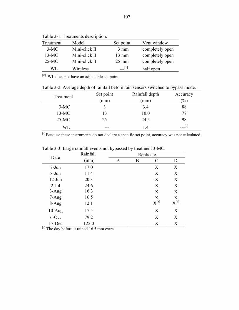
107
Table 3-1. Treatments description. Treatment Model Set point Vent window 3-MC Mini-click II 3 mm completely open 13-MC Mini-click II 13 mm completely open 25-MC Mini-click II 25 mm completely open WL Wireless ---[z] half open [z] WL does not have an adjustable set point. Table 3-2. Average depth of rainfall before rain sensors switched to bypass mode.
Set point Rainfall depth Accuracy Treatment (mm) (mm) (%)
3-MC 3 3.4 88 13-MC 13 10.0 77 25-MC 25 24.5 98
WL --- 1.4 ---[z] [z] Because these instruments do not declare a specific set point, accuracy was not calculated.
Table 3-3. Large rainfall events not bypassed by treatment 3-MC. Rainfall Replicate Date (mm) A B C D
7-Jun 17.0 X X 8-Jun 11.4 X X 12-Jun 20.3 X X 2-Jul 24.6 X X
3-Aug 16.3 X X 7-Aug 16.5 X X 8-Aug 12.1 X[z] X[z] 10-Aug 17.5 X X 6-Oct 79.2 X X
17-Dec 122.0 X X [z] The day before it rained 16.5 mm extra.
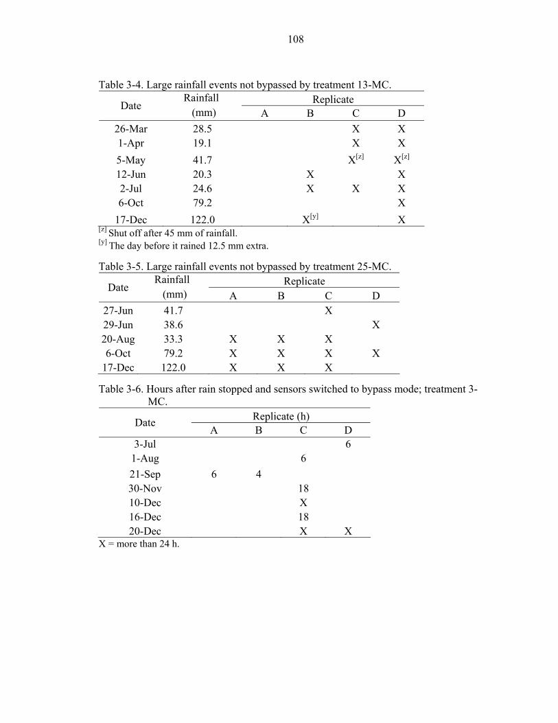
108
Table 3-4. Large rainfall events not bypassed by treatment 13-MC.
Rainfall Replicate Date (mm) A B C D 26-Mar 28.5 X X 1-Apr 19.1 X X 5-May 41.7 X[z] X[z] 12-Jun 20.3 X X 2-Jul 24.6 X X X 6-Oct 79.2 X
17-Dec 122.0 X[y] X [z] Shut off after 45 mm of rainfall. [y] The day before it rained 12.5 mm extra. Table 3-5. Large rainfall events not bypassed by treatment 25-MC.
Rainfall Replicate Date (mm) A B C D 27-Jun 41.7 X 29-Jun 38.6 X 20-Aug 33.3 X X X 6-Oct 79.2 X X X X
17-Dec 122.0 X X X Table 3-6. Hours after rain stopped and sensors switched to bypass mode; treatment 3-
MC. Replicate (h) Date
A B C D 3-Jul 6
1-Aug 6 21-Sep 6 4 30-Nov 18 10-Dec X 16-Dec 18 20-Dec X X
X = more than 24 h.
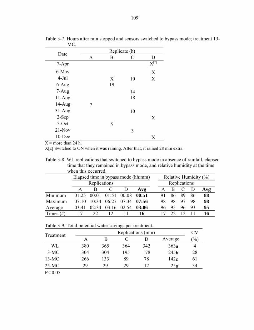
109
Table 3-7. Hours after rain stopped and sensors switched to bypass mode; treatment 13-
MC. Replicate (h) Date
A B C D 7-Apr X[z] 6-May X 4-Jul X 10 X
6-Aug 19 7-Aug 14 11-Aug 18 14-Aug 7 31-Aug 10 2-Sep X 5-Oct 5
21-Nov 3 10-Dec X
X = more than 24 h. X[z] Switched to ON when it was raining. After that, it rained 28 mm extra. Table 3-8. WL replications that switched to bypass mode in absence of rainfall, elapsed
time that they remained in bypass mode, and relative humidity at the time when this occurred.
Elapsed time in bypass mode (hh:mm) Relative Humidity (%)Replications Replications
A B C D Avg A B C D AvgMinimum 01:25 00:01 01:51 00:08 00:51 91 86 89 86 88Maximum 07:10 10:34 06:27 07:34 07:56 98 98 97 98 98Average 03:41 02:34 03:16 02:54 03:06 96 95 96 93 95Times (#) 17 22 12 11 16 17 22 12 11 16 Table 3-9. Total potential water savings per treatment.
Replications (mm) CV Treatment A B C D Average (%)
WL 380 365 364 342 363 a 4 3-MC 304 304 195 178 245 b 28 13-MC 266 133 89 78 142 c 61 25-MC 29 29 29 12 25 d 34 P< 0.05
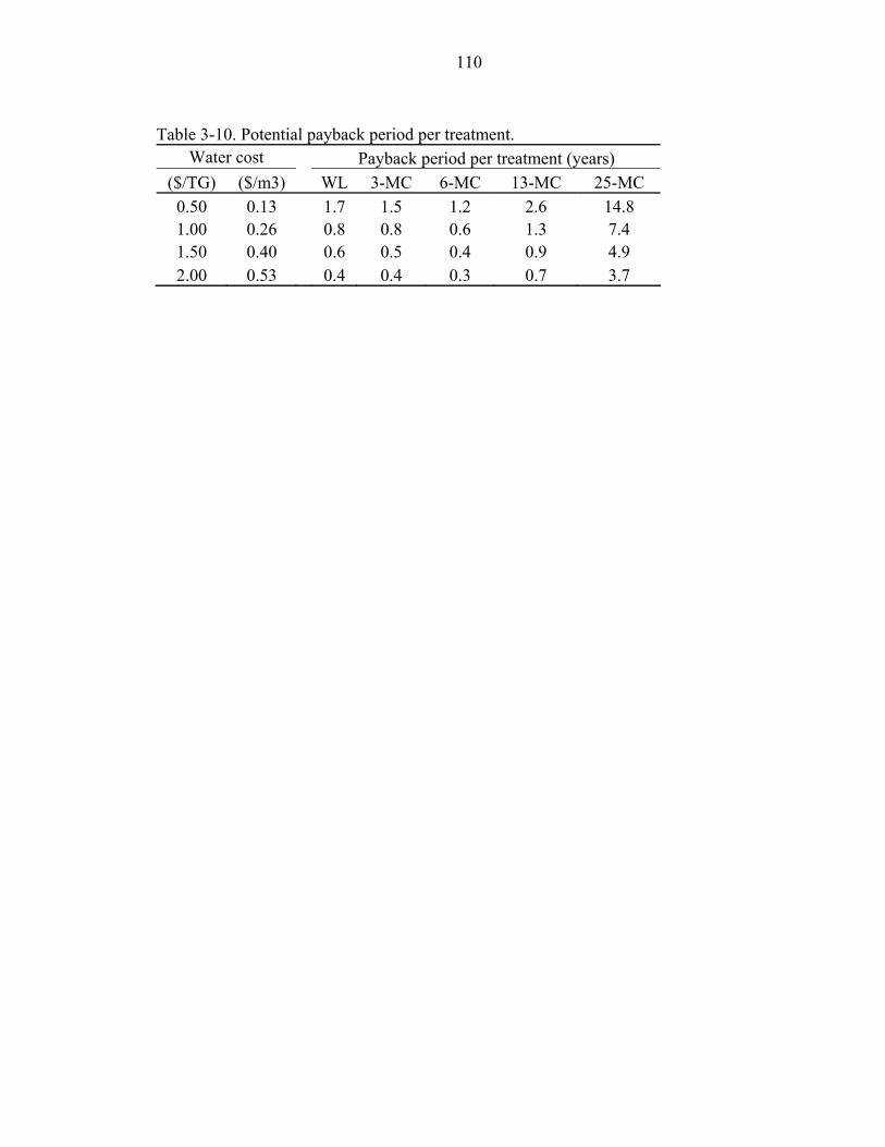
110
Table 3-10. Potential payback period per treatment.
Water cost Payback period per treatment (years) ($/TG) ($/m3) WL 3-MC 6-MC 13-MC 25-MC
0.50 0.13 1.7 1.5 1.2 2.6 14.8 1.00 0.26 0.8 0.8 0.6 1.3 7.4 1.50 0.40 0.6 0.5 0.4 0.9 4.9 2.00 0.53 0.4 0.4 0.3 0.7 3.7
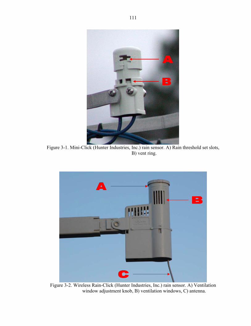
111
Figure 3-1. Mini-Click (Hunter Industries, Inc.) rain sensor. A) Rain threshold set slots,
B) vent ring.
Figure 3-2. Wireless Rain-Click (Hunter Industries, Inc.) rain sensor. A) Ventilation
window adjustment knob, B) ventilation windows, C) antenna.

112
Figure 3-3. The expanding material of a rain shut-off switch.
Figure 3-4. Rain sensor experiment layout: A) Wireless Rain-Click rain sensors, B) Mini-
Click rain sensors, C) Wireless Rain-Click receivers, D) multiplexers, E) CR 10X datalogger.
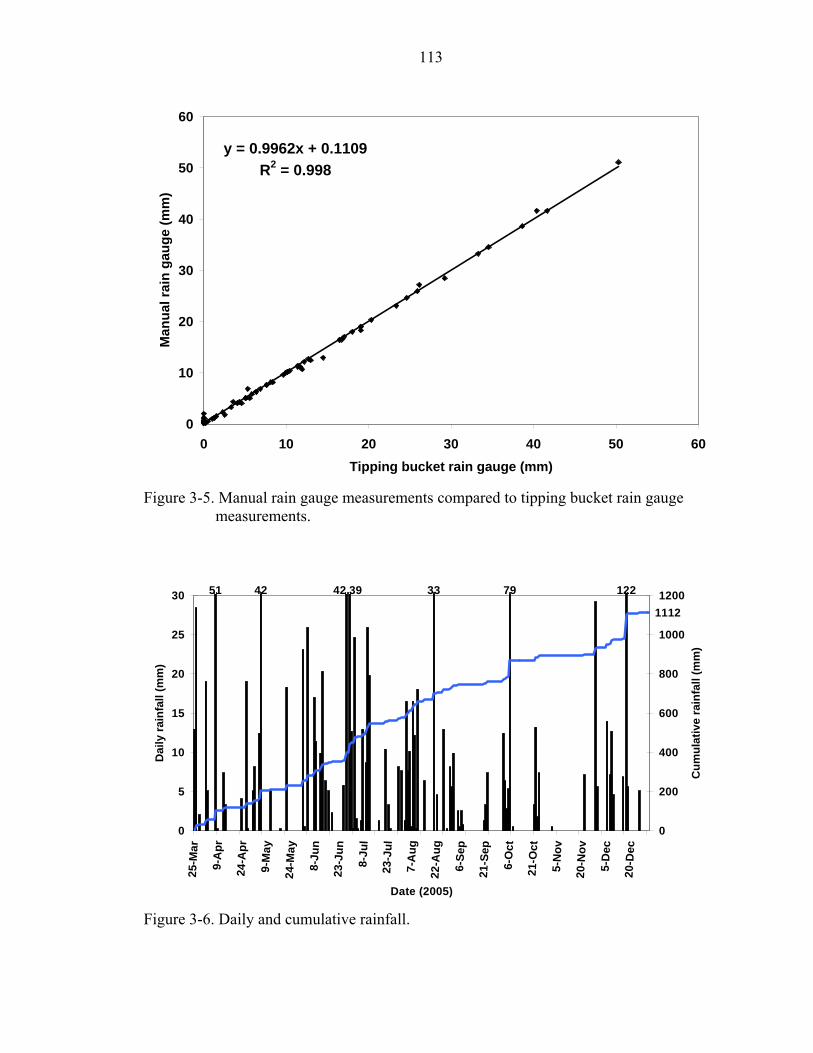
113
y = 0.9962x + 0.1109R2 = 0.998
0
10
20
30
40
50
60
0 10 20 30 40 50 60Tipping bucket rain gauge (mm)
Man
ual r
ain
gaug
e (m
m)
Figure 3-5. Manual rain gauge measurements compared to tipping bucket rain gauge
measurements.
3942 12279334251
1112
0
5
10
15
20
25
30
25-M
ar
9-A
pr
24-A
pr
9-M
ay
24-M
ay
8-Ju
n
23-J
un
8-Ju
l
23-J
ul
7-A
ug
22-A
ug
6-Se
p
21-S
ep
6-O
ct
21-O
ct
5-N
ov
20-N
ov
5-D
ec
20-D
ec
Date (2005)
Dai
ly ra
infa
ll (m
m)
0
200
400
600
800
1000
1200
Cum
ulat
ive
rain
fall
(mm
)
Figure 3-6. Daily and cumulative rainfall.

114
81a
43b
30c
8d0
10
20
30
40
50
60
70
80
90
24-Mar 24-Apr 25-May 25-Jun 26-Jul 26-Aug 26-Sep 27-Oct 27-Nov 28-DecDate
Cum
ulat
ive
even
ts in
byp
ass
mod
e
WL 3-MC 13-MC 25-MC
Figure 3-7. Cumulative number of times rain sensors switched to bypass mode; average per treatment. Different letters indicate a significant difference by Duncan’s Multiple Range Test (P<0.05)
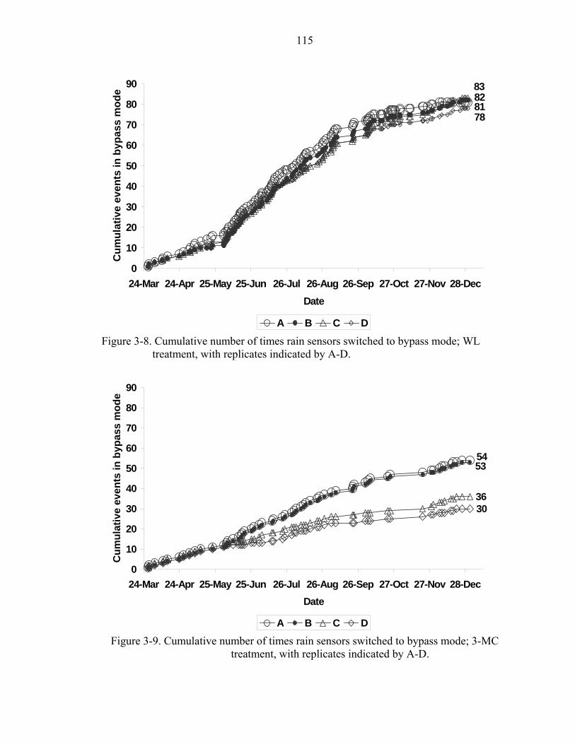
115
818283
78
0
10
20
30
40
50
60
70
80
90
24-Mar 24-Apr 25-May 25-Jun 26-Jul 26-Aug 26-Sep 27-Oct 27-Nov 28-DecDate
Cum
ulat
ive
even
ts in
byp
ass
mod
e
A B C D
Figure 3-8. Cumulative number of times rain sensors switched to bypass mode; WL treatment, with replicates indicated by A-D.
5453
3630
0
10
20
30
40
50
60
70
80
90
24-Mar 24-Apr 25-May 25-Jun 26-Jul 26-Aug 26-Sep 27-Oct 27-Nov 28-DecDate
Cum
ulat
ive
even
ts in
byp
ass
mod
e
A B C D
Figure 3-9. Cumulative number of times rain sensors switched to bypass mode; 3-MC treatment, with replicates indicated by A-D.
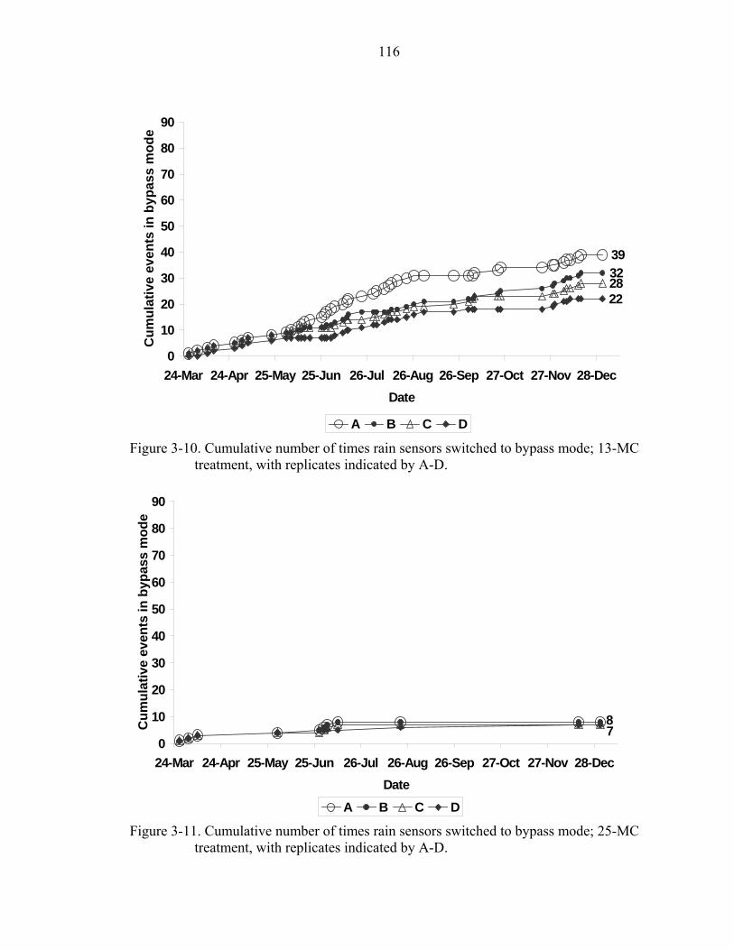
116
39322822
0
10
20
30
40
50
60
70
80
90
24-Mar 24-Apr 25-May 25-Jun 26-Jul 26-Aug 26-Sep 27-Oct 27-Nov 28-DecDate
Cum
ulat
ive
even
ts in
byp
ass
mod
e
A B C D
Figure 3-10. Cumulative number of times rain sensors switched to bypass mode; 13-MC treatment, with replicates indicated by A-D.
87
0
10
20
30
40
50
60
70
80
90
24-Mar 24-Apr 25-May 25-Jun 26-Jul 26-Aug 26-Sep 27-Oct 27-Nov 28-DecDate
Cum
ulat
ive
even
ts in
byp
ass
mod
e
A B C D
Figure 3-11. Cumulative number of times rain sensors switched to bypass mode; 25-MC treatment, with replicates indicated by A-D.
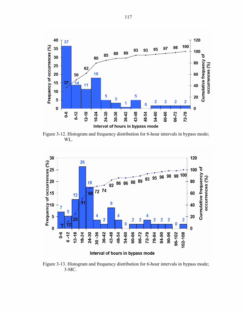
117
Figure 3-12. Histogram and frequency distribution for 6-hour intervals in bypass mode;
WL.
Figure 3-13. Histogram and frequency distribution for 6-hour intervals in bypass mode;
3-MC.
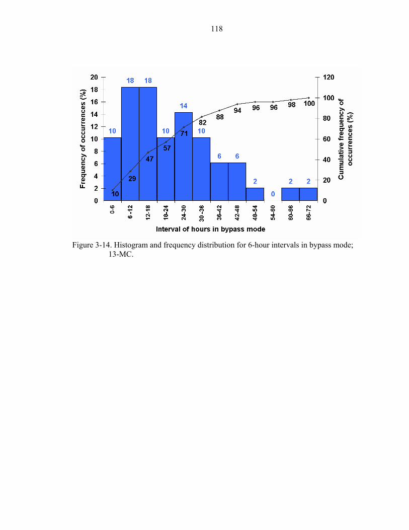
118
Figure 3-14. Histogram and frequency distribution for 6-hour intervals in bypass mode;
13-MC.

119
CHAPTER 4 GRANULAR MATRIX SENSOR PERFORMANCE COMPARED TO
TENSIOMETER IN A SANDY SOIL
Numerous methods exist to measure soil water content, including gravimetric
measurements, neutron scattering, resistance blocks, tensiometers, and granular matrix
sensors (GMS). These methods are fairly common, some of them have been used for
several decades, and continue to be used extensively in irrigation scheduling (Gardner,
1986; Seyfried, 1993; Leib et al., 2002; Leib et al., 2003; Or, 2001).
In this research, two of these methods were compared, tensiometers and granular
matrix sensors (GMS), in a sandy soil.
Tensiometers
Tensiometers have been used for many years to measure soil water tension in the
field. Of all the methods available for monitoring water potential for irrigation, the
tensiometers are perhaps the most widely used (Campbell and Mulla, 1990).
A tensiometer (Figure 4-1) consists of a sealed, water-filled tube with a permeable
porous cup on one end, an airtight seal on the other end and some means of measuring
tension (a gauge, manometer, or electronic pressure transducer). The device is installed in
the soil with the ceramic tip in close contact with the soil at the desired depth. Water is
pulled out through the ceramic tip into the soil creating a tension in the closed tube. As
the soil is re-wetted (e.g., from rain or irrigation), the tension gradient reduces, causing
water to flow into the ceramic tip (Ley et al., 2000). At equilibrium, the water pressure
(tension) in the tensiometer is equal in magnitude to the soil matric potential (Cassell and
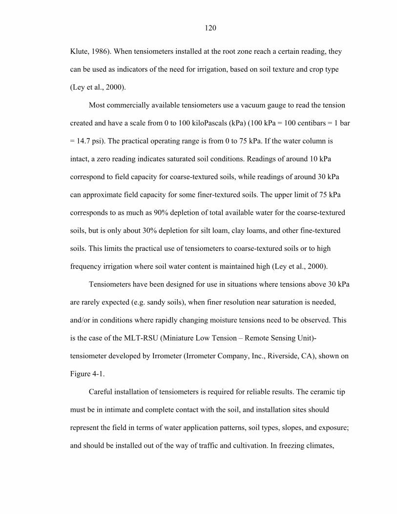
120
Klute, 1986). When tensiometers installed at the root zone reach a certain reading, they
can be used as indicators of the need for irrigation, based on soil texture and crop type
(Ley et al., 2000).
Most commercially available tensiometers use a vacuum gauge to read the tension
created and have a scale from 0 to 100 kiloPascals (kPa) (100 kPa = 100 centibars = 1 bar
= 14.7 psi). The practical operating range is from 0 to 75 kPa. If the water column is
intact, a zero reading indicates saturated soil conditions. Readings of around 10 kPa
correspond to field capacity for coarse-textured soils, while readings of around 30 kPa
can approximate field capacity for some finer-textured soils. The upper limit of 75 kPa
corresponds to as much as 90% depletion of total available water for the coarse-textured
soils, but is only about 30% depletion for silt loam, clay loams, and other fine-textured
soils. This limits the practical use of tensiometers to coarse-textured soils or to high
frequency irrigation where soil water content is maintained high (Ley et al., 2000).
Tensiometers have been designed for use in situations where tensions above 30 kPa
are rarely expected (e.g. sandy soils), when finer resolution near saturation is needed,
and/or in conditions where rapidly changing moisture tensions need to be observed. This
is the case of the MLT-RSU (Miniature Low Tension – Remote Sensing Unit)-
tensiometer developed by Irrometer (Irrometer Company, Inc., Riverside, CA), shown on
Figure 4-1.
Careful installation of tensiometers is required for reliable results. The ceramic tip
must be in intimate and complete contact with the soil, and installation sites should
represent the field in terms of water application patterns, soil types, slopes, and exposure;
and should be installed out of the way of traffic and cultivation. In freezing climates,
121
tensiometers must be insulated or removed during winter months, because it takes only a
small frost to knock the vacuum gauges out of calibration (Ley et al., 2000).
Granular Matrix Sensors
The GMS (Figure 4-2) is a device that measures soil electrical resistance, that can
be converted to soil water tension (SWT), either using a calibration formula provided in
the literature for sandy soils (Irmak and Haman, 2001) and silt loam soils (Eldredge et al.,
1993), or calibrating them for a specific soil type (Hanson et al., 2000b; Intrigliolo and
Castel, 2004).
Since the development of the GMS, many researchers (Eldredge et al., 1993;
Mitchell and Shock, 1996; Bausch and Bernard, 1996) have used it in agricultural water
management, including irrigation scheduling. However, some limitations in its use have
been found. For example, in coarse–textured soils (e.g. sand) a lack of soil–sensor
interface might be observed, and consequently may lead to incorrect estimation of SWT
(Irmak and Haman, 2001). Also, GMS has a high uncertainty in the wet range and do not
respond to changes at a SWT lower than 10 kPa and, therefore, may not be a suitable tool
in those cases where irrigation practices maintain a low SWT (Irmak and Haman, 2001;
Taber et al., 2002: Intrigliolo and Castel, 2004). In addition, McCann et al. (1992) found
that GMS has a hysteretic behavior when induced to rapid drying or partial rewetting of
the soil, which could affect the performance of the GMS in estimating the actual soil
water status. Moreover, there is also evidence that the most important drawback on its use
for irrigation scheduling is the high variability of its readings (CV of 35–50%), increasing
at the lower SWT range (Taber et al., 2002; Intrigliolo and Castel, 2004). Finally,
calibration appears to be exclusive for each individual sensor (Egbert et al., 1992; Hanson
et al., 2000b; Leib et al., 2003; Intrigliolo and Castel, 2004).
122
In spite of all these limitations, GMS may be useful when a relative indication of
soil wetness is needed, as indicated by reports of their successful use for irrigation
scheduling in onion (Shock et al., 1998a), potato (Shock et al., 1998b), tomato, and
walnut trees (Hanson et al., 2000a).
GMS – Tensiometer Comparison
Previous research found that GMSs functioned consistently over a range of SWT
from 10 kPa to 200 kPa (Hanson et al., 2000a; Leib et al., 2003; Intrigliolo and Castel,
2004). So, GMS can operate in a drier range than tensiometers, but with a lower
resolution at the wet end of SWT (Egbert et al., 1992; Irmak and Haman, 2001). This is
an important limitation for the use of GMS in the predominantly coarse-textured soils of
Florida.
Bausch and Bernard (1996) evaluated the validity of the granular matrix sensor
SWT values calculated using Thomson and Armstrong (1987) and Shock et al. (1996)
calibration equations with the tensiometer-measured SWT. However, both equations
underestimated SWT for sandy clay loam soil. Thomson et al. (1996) compared Thomson
and Armstrong (1987) and McCann et al. (1992) equations and indicated that the
equations deviated significantly for estimating SWT.
Objectives
The objectives of this research were to: a) compare GMS to tensiometer readings
on a sandy soil, b) establish a relationship between them, if any, and c) evaluate the
performance of the GMSs in a sandy soil.
Materials and Methods
The experiment was conducted in 2004 in the Water Resources Lab at the
University of Florida, Gainesville, Florida. Three PVC cylinders [19.14 L (0.30 m high ×
123
0.285 m diameter)], were hand-packed with an Arredondo fine sand (loamy, siliceous,
semiactive, hyperthermic Grossarenic Paleudults) (USDA, 2003), taken from the field
where the soil moisture sensor experiment was carried out.
Experimental Set-Up
In each PVC cylinder, three 200SS model Watermark GMSs (Irrometer Company,
Inc., Riverside, CA) were installed vertically, in a uniformly spaced pattern. (Prior to
installation, GMSs were immersed in water for two days, according to manufacturer
instructions.) A temperature sensor (Irrometer Company, Inc., Riverside, Calif.) was
installed in the center of the PVC cylinders to correct the GMS readings. In addition,
three MLT-RSU model Tensiometers (Irrometer Company, Inc., Riverside, CA),
hereafter-called tensiometers, were also placed near the GMSs. Finally, a capacitance
ECH2O probe (Decagon Devices, Inc., Pullman, WA) was also placed in each PVC
cylinder. Figures 4-1 through 4-4 show pictures of the devices. GMSs were placed with
their center at 9 cm soil depth. All other devices were installed with their sensing section
at the depth of GMS centers. The experimental layout is shown in Figure 4-5.
ECH2O Probes Calibration
Before the experiment was carried out, the ECH2O probes were calibrated through
the thermogravimetric soil sampling method (Gardner, 1986). Undisturbed soil samples
were collected (using a core sampler of 137.4 cm3) from each PVC cylinder at the same
depth where ECH2O probes were placed. Samples were taken from a saturated through a
dry condition (28.4% to 4.8% of VMC, respectively, based on gravimetric data).
The samples were weighed and then oven-dried at 104°C for 24 h. Then, the dry
samples were re-weighed. Percent soil water content on a dry mass or gravimetric basis,
Pw, was determined by the following formula:

124
100x weightdry sample
weightdry sample - weight samplewetPw = [4-1]
To convert from a gravimetric basis to water content on a volumetric basis, Pv, the
gravimetric soil water content was multiplied by the soil bulk density (BD):
Pv = Pw x BD [4-2]
and soil bulk density was determined by:
dry soil of volume dry sample of weightBD = [4-3]
The volumetric soil water content of each sample was then compared to the ECH2O
probe readings at the same date and time when the samples were taken and, then, these
data were compared to calibrate the ECH2O probe readings.
Treatments
All three PVC cylinders had a ceramic porous plate placed at the bottom to
withdraw water from the cylinders to accelerate drying. Suction was applied, using a
vacuum pump connected to the porous plate. A different initial suction time was applied
to each cylinder to create different rates of soil drying, defining the treatments (Table 4-
1): 0, 5, 15, and 50 min for treatments T0, T5, T15, and T50, respectively.
Data
The tensiometers, GMSs, and temperature sensor were connected to a Watermark
Monitor (Figure 4-6). This is a data logger developed by Irrometer (Irrometer Company,
Inc., Riverside, Calif.), which includes an automatic temperature compensation of the soil
moisture readings, and gives GMS and tensiometer readings in kPa. The ECH2O probes
were connected to a HOBO Micro Station (Figure 4-7) data logger (Onset Computer
Corporation, Bourne, MA). All sensor data were recorded every 15 minutes.

125
Results and Discussion
Calibration of the ECH2O Probe
Data from the three ECH2O probes compared to thermogravimetric measurements
is given in Figure 4-8. It can be seen that ECH2O measurements and gravimetric
measurements were highly correlated (R2 = 0.95). However, the ECH20 probes under
predicted the gravimetric water content by about 20% as seen in Figure 4-8.
GMSs versus Tensiometers.
In previous research, when comparing GMS with other SMC-methods, authors
took electrical resistance measurements from GMS, and then converted these data to
tension, through calibration equations (Irmak and Haman, 2001; Eldredge et al., 1993;
Hanson et al., 2000b). In this research, the Watermark Monitor-datalogger gave the GMS
readings expressed immediately in tension, so no conversion with a calibration curve was
theoretically necessary.
The results from the different treatments are displayed in Figures 4-9 through 4-16.
It can be seen that the curves of GMSs and tensiometers followed a similar trend, but
tension readings were different. Their soil water tension curves crossed at average values
in the range of 5.8 through 6.7 kPa, depending on the treatment, with an overall average
of 6.2 kPa (Table 4-2). At tensions less than this level, GMSs gave lower tensions than
the tensiometers, and the opposite occurred at tensions higher than these values, where
GMSs showed a consistently drier estimate of the soil moisture content compared to
tensiometers.
Relating the average of GMS and tensiometer readings (Figure 4-17), a coefficient
of determination of R2=0.9582 was found for a linear relationship between them, and a
coefficient of determination of R2=0.9916 for a logarithmic relationship between them.

126
Previous studies reported that GMSs do not respond accurately at tensions less than 10
kPa (Egbert et al., 1992; Irmak and Haman, 2001). Moreover, Eldredge et al. (1993) did
not include these data when performing their analysis. In the present experiment, GMS
values at tensions less than 7 kPa were not stable, showing fluctuations between ±1kPa
(Figures 4-13 and to 4-14). When replotting the average of GMS and tensiometer
readings without including tensions below 10 kPa (Figure 4-18) the coefficient of
determination increased to R2=0.9809 for a linear relationship, and increased to
R2=0.9956 for a logarithmic relationship.
In the sandy soils of North-Central Florida, the trigger point to start an irrigation
cycle is often reported as 10-30 kPa. If that is the case, when tensiometers were reading
10 kPa, GMSs were reading between 17 and 23 kPa, and an average of 20 kPa. This
could have a major consequence if an automatic irrigation system is controlled by a
GMS, because is highly probable that they would allow irrigation cycles when actually
they are not necessary, which is exactly what happened with the GMS-controlled
irrigation in Chapter 2. According to these results, it is evident that calibration of GMS
units in this type of soil is necessary.
Conclusions
Tension readings from tensiometers and GMSs were the same, at levels close to 6.2
kPa. Below this tension, GMSs readings were lower than those from tensiometers, and
the opposite occurred at tensions higher than this value. At the same time as tensions
continued to increase, the difference between both methods increased. In addition, GMS
readings below 7 kPa were not stable, fluctuating between ±1kPa.
The set point (kPa) to initiate irrigation could be of great consequence regarding
water use efficiency, when GMSs are set to control an automatic irrigation system.

127
According to these results, it was evident that calibration of GMS units in this type of soil
is necessary to obtain readings closer to reality, and achieve adequate irrigation
management.
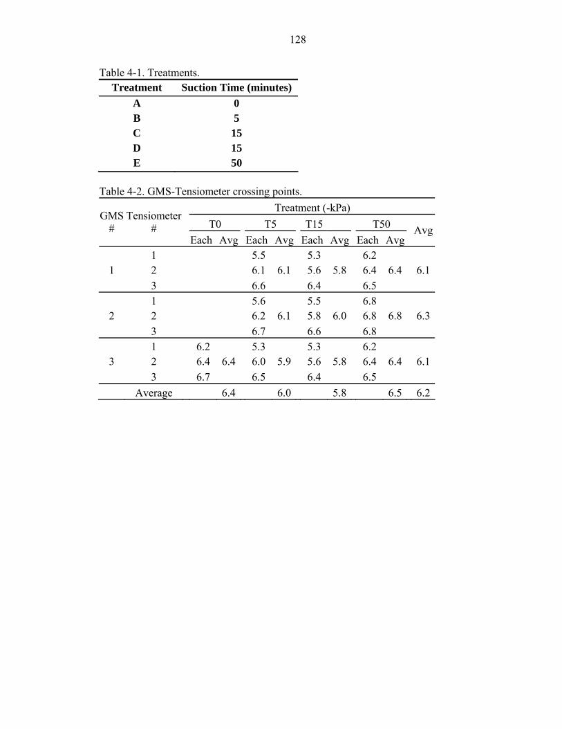
128
Table 4-1. Treatments. Treatment Suction Time (minutes)
A 0 B 5 C 15 D 15 E 50
Table 4-2. GMS-Tensiometer crossing points.
Treatment (-kPa) T0 T5 T15 T50
GMS #
Tensiometer #
Each Avg Each Avg Each Avg Each Avg Avg
1 5.5 5.3 6.2 1 2 6.1 6.1 5.6 5.8 6.4 6.4 6.1 3 6.6 6.4 6.5 1 5.6 5.5 6.8 2 2 6.2 6.1 5.8 6.0 6.8 6.8 6.3 3 6.7 6.6 6.8 1 6.2 5.3 5.3 6.2 3 2 6.4 6.4 6.0 5.9 5.6 5.8 6.4 6.4 6.1 3 6.7 6.5 6.4 6.5 Average 6.4 6.0 5.8 6.5 6.2
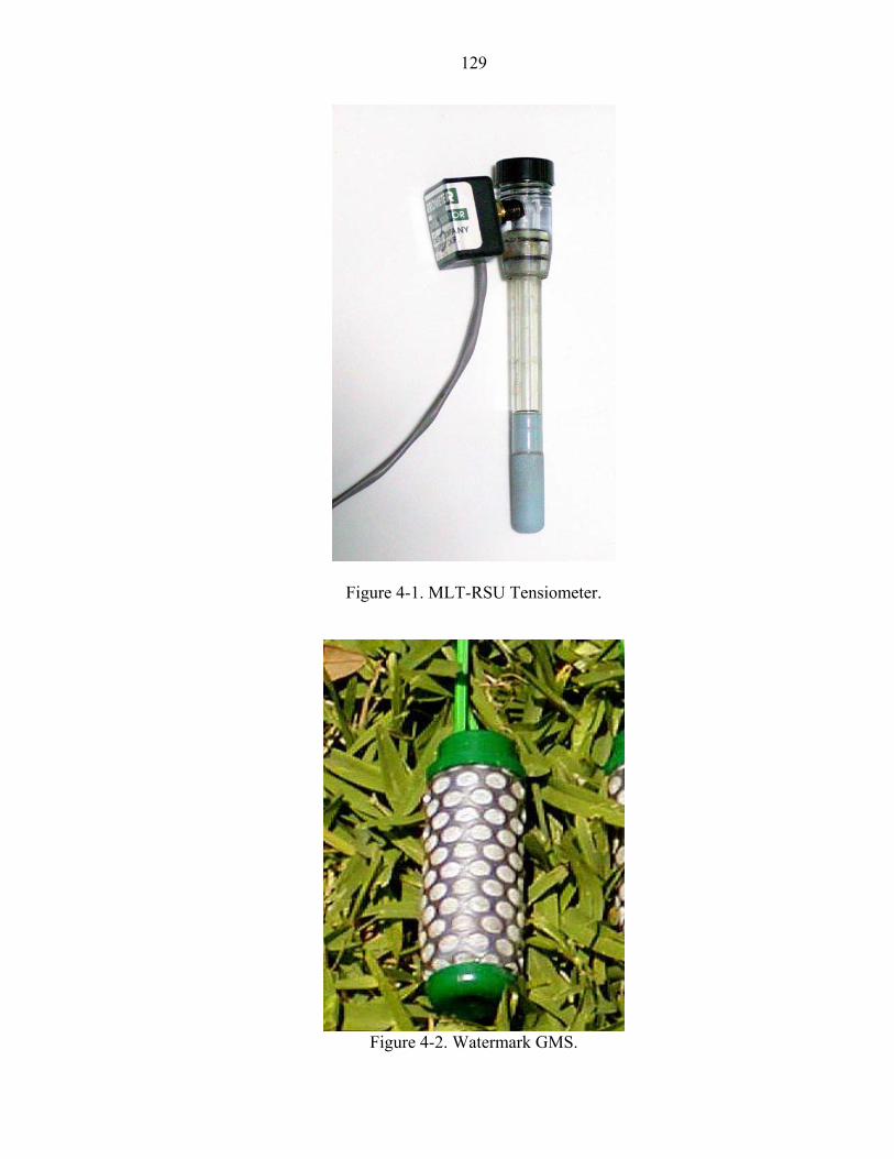
129
Figure 4-1. MLT-RSU Tensiometer.
Figure 4-2. Watermark GMS.
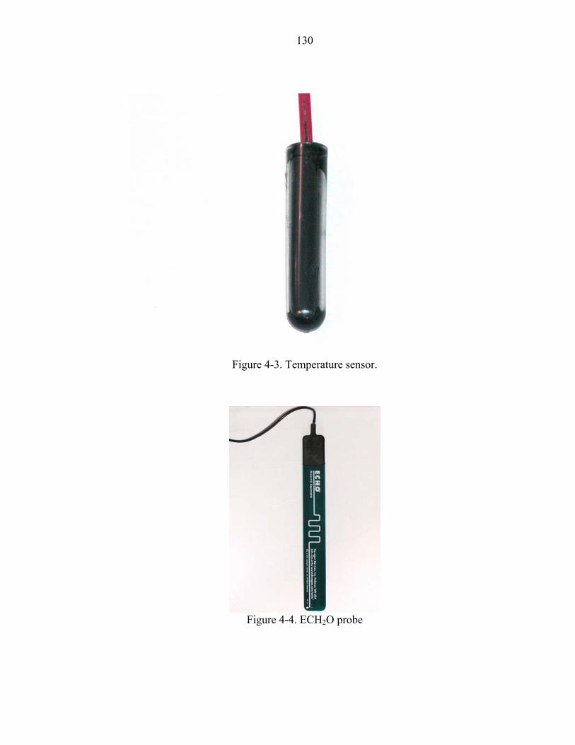
130
Figure 4-3. Temperature sensor.
Figure 4-4. ECH2O probe

131
Figure 4-5. Experimental layout (top view). A) Tensiometers, B) Granular matrix sensors, C) ECH2O probe, and D) Thermometer.
C
AA
A
B
D
B
B
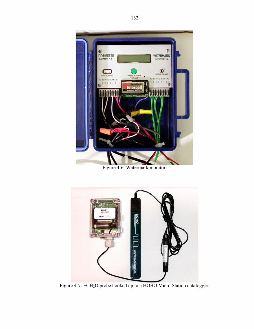
132
Figure 4-6. Watermark monitor.
Figure 4-7. ECH2O probe hooked up to a HOBO Micro Station datalogger.
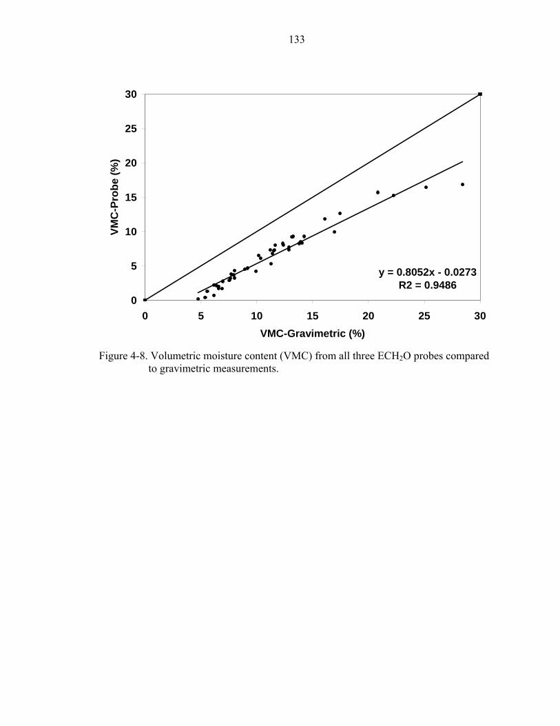
133
y = 0.8052x - 0.0273R2 = 0.9486
0
5
10
15
20
25
30
0 5 10 15 20 25 30VMC-Gravimetric (%)
VMC
-Pro
be (%
)
Figure 4-8. Volumetric moisture content (VMC) from all three ECH2O probes compared
to gravimetric measurements.
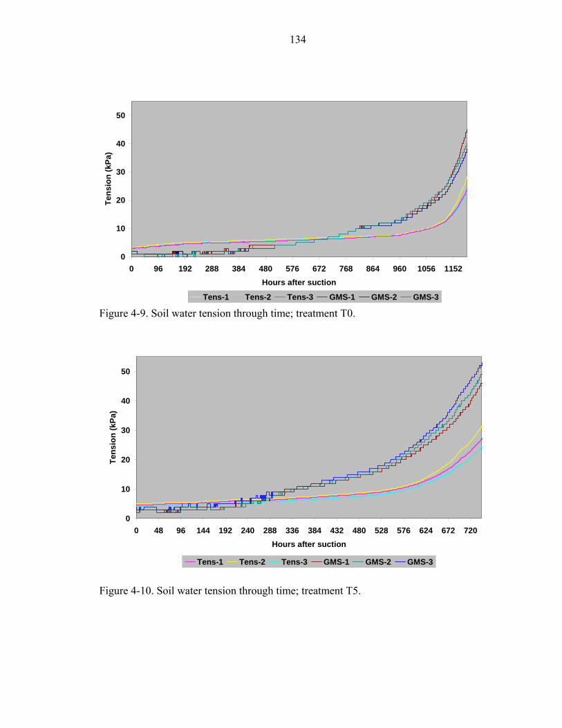
134
0
10
20
30
40
50
0 96 192 288 384 480 576 672 768 864 960 1056 1152Hours after suction
Tens
ion
(kPa
)
Tens-1 Tens-2 Tens-3 GMS-1 GMS-2 GMS-3 Figure 4-9. Soil water tension through time; treatment T0.
0
10
20
30
40
50
0 48 96 144 192 240 288 336 384 432 480 528 576 624 672 720Hours after suction
Tens
ion
(kPa
)
Tens-1 Tens-2 Tens-3 GMS-1 GMS-2 GMS-3 Figure 4-10. Soil water tension through time; treatment T5.

135
0
10
20
30
40
50
0 48 96 144 192 240 288 336 384 432 480 528 576 624 672 720 768 816Hours after suction
Tens
ion
(kPa
)
Tens-1 Tens-2 Tens-3 GMS-1 GMS-2 GMS-3 Figure 4-11. Soil water tension through time; treatment T15.
0
10
20
30
40
50
0 48 96 144 192 240Hours after suction
Tens
ion
(kPa
)
Tens-1 Tens-2 Tens-3 GMS-1 GMS-2 GMS-3 Figure 4-12. Soil water tension through time; treatment T50.
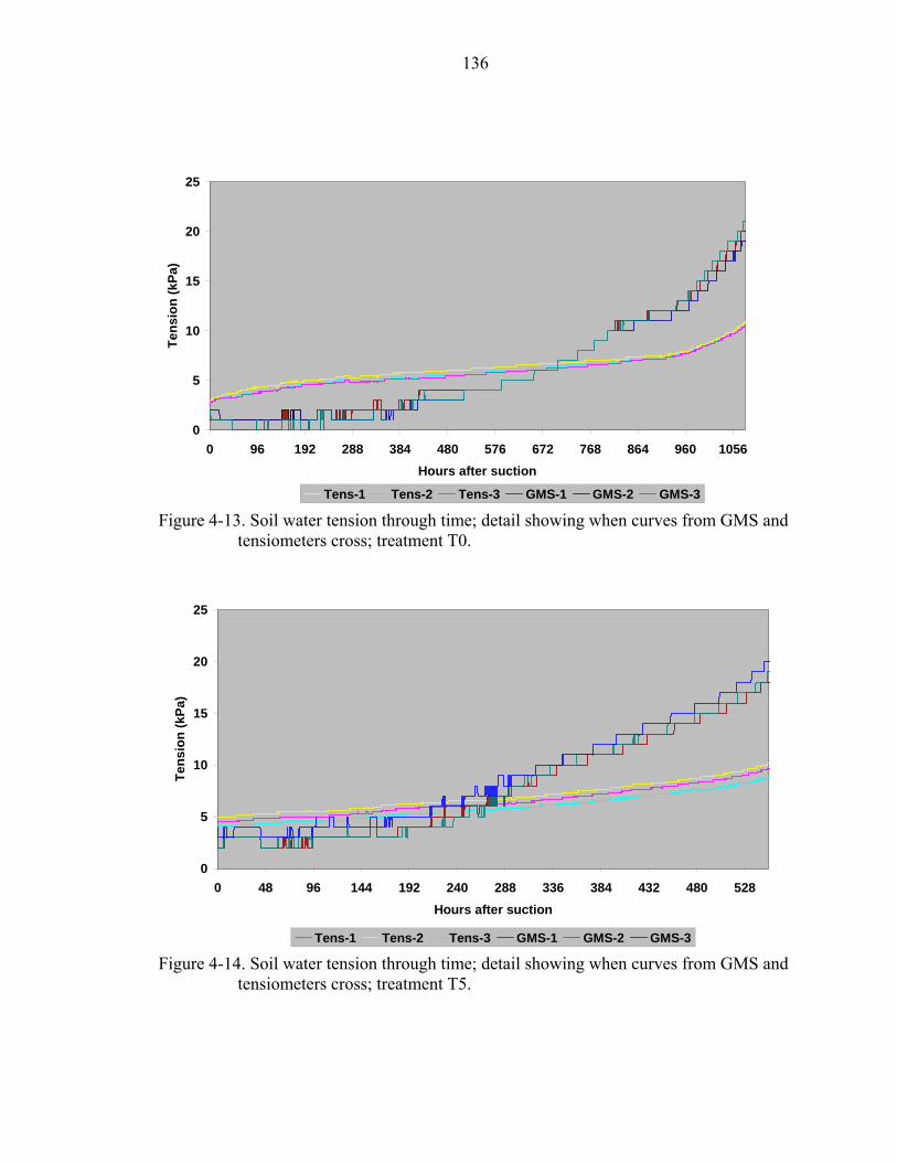
136
0
5
10
15
20
25
0 96 192 288 384 480 576 672 768 864 960 1056Hours after suction
Tens
ion
(kPa
)
Tens-1 Tens-2 Tens-3 GMS-1 GMS-2 GMS-3 Figure 4-13. Soil water tension through time; detail showing when curves from GMS and
tensiometers cross; treatment T0.
0
5
10
15
20
25
0 48 96 144 192 240 288 336 384 432 480 528Hours after suction
Tens
ion
(kPa
)
Tens-1 Tens-2 Tens-3 GMS-1 GMS-2 GMS-3 Figure 4-14. Soil water tension through time; detail showing when curves from GMS and
tensiometers cross; treatment T5.
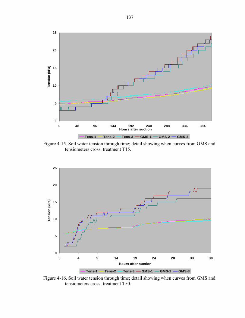
137
0
5
10
15
20
25
0 48 96 144 192 240 288 336 384Hours after suction
Tens
ion
(kPa
)
Tens-1 Tens-2 Tens-3 GMS-1 GMS-2 GMS-3 Figure 4-15. Soil water tension through time; detail showing when curves from GMS and
tensiometers cross; treatment T15.
0
5
10
15
20
25
0 4 9 14 19 24 28 33 38Hours after suction
Tens
ion
(kPa
)
Tens-1 Tens-2 Tens-3 GMS-1 GMS-2 GMS-3 Figure 4-16. Soil water tension through time; detail showing when curves from GMS and
tensiometers cross; treatment T50.
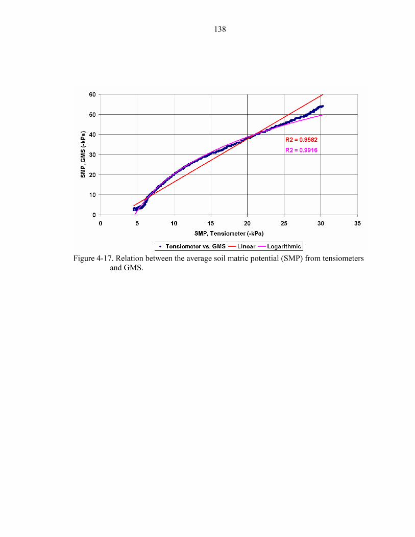
138
Figure 4-17. Relation between the average soil matric potential (SMP) from tensiometers
and GMS.
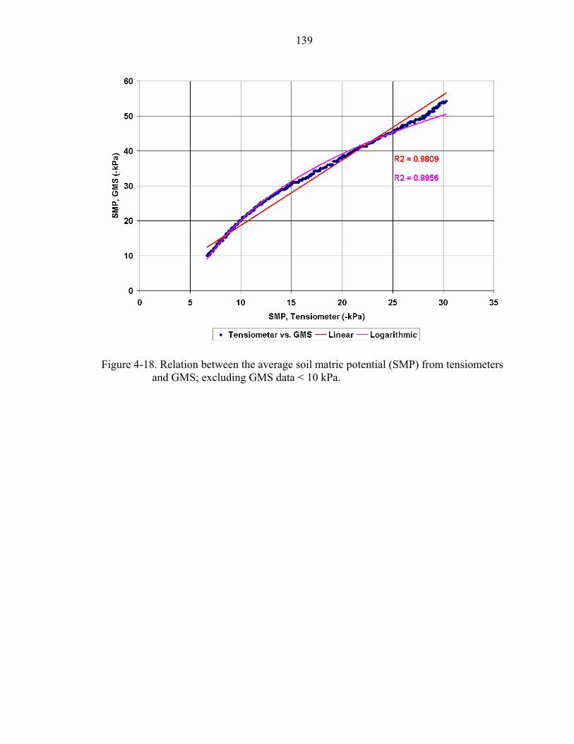
139
Figure 4-18. Relation between the average soil matric potential (SMP) from tensiometers
and GMS; excluding GMS data < 10 kPa.

140
CHAPTER 5 CONCLUSIONS AND FUTURE WORK
Conclusions
The goals of this research were to find out if different SMS-systems (sensor with a
proprietary controller) could reduce irrigation water application–while maintaining
acceptable turf quality–compared to current practices and, on the other hand, to collect
evidence related to RS performance and reliability. The main objectives of this
experiment were to quantify differences in irrigation water use and turf quality between:
1) a soil moisture sensor-based irrigation system compared to a time-based scheduling, 2)
different commercial irrigation soil moisture sensor (SMSs), and 3) a time-based
scheduling system with or without a rain sensor (RS). The secondary objectives were to:
a) evaluate the reliability of two commercially available expanding disk RS-types, b)
quantify the amount of water that RSs could save compared to time-based irrigation
schedules without RS, and c) estimate the payback period of RSs at different set points.
Results showed that no significant differences in turfgrass quality among
treatments were detected, which was evidenced by good quality in non-irrigated plots.
This was a consequence of the high frequency rainfall events and large amount of
cumulative precipitation that prevailed during the time frame of this research and, on the
other hand, because of the documented characteristics of bermudagrass as a drought-
tolerant plant.
Regarding the time-based treatments, 2-WORS (without-rain-sensor) used
significantly (52%) more water than 2-WRS (with-rain-sensor), showing the importance
141
not only for the presence but also for the need of a well-maintained rain shut-off device in
all automated irrigation systems. However, treatment 2-WRS was fairly well managed
and conservative, compared to homeowners’ actual operation practices, so “real” water
savings on residential landscapes could be even larger.
It was inferred that, in general, SMS-based treatments were able to follow and
detect fairly well when sufficient rain occurred, overriding pre-set irrigation cycles, and
allowing the rest of them to run when necessary.
SMS-based treatments were, on average, significantly more efficient as a means to
save water than the time-based treatments. However, not all SMSs tested performed the
same. Sensors from brand Irrometer always applied significantly more water than the
other brands/treatments in every frequency. All the other brands (AC, RB, and WW)
recorded significant irrigation water savings compared to 2-WRS, which ranged from
54% to 88%, depending on the irrigation frequency. When compared to 2-WORS, the
differences increased, and ranged from 69% to 92% in water savings.
Therefore SMS-systems represent a promising technology, because of the water
savings that they can accomplish, while maintaining an acceptable turfgrass quality. The
correct choice of a SMS should take into consideration features like its technology,
response-time, irrigation scheduling strategy, and cost, among other aspects.
Regarding the RS treatments, on average, treatments WL, 3-MC, 13-MC, and 25-
MC responded close to their rainfall set points (1.4, 3.4, 10.0, and 24.5 mm,
respectively). However, some replications showed erratic behavior through time.
The number of times that these sensors shut off irrigation was inversely
proportional to the magnitude of their set point (81, 43, 30, and 8 times, respectively)
142
with potential water savings following a similar trend (363, 245, 142, and 25 mm,
respectively).
Under the relatively wet testing conditions typical to Florida, the payback period of
the RSs tested could be less than a year, except for 25-MC (around 7 years).
Consequently, RSs are strongly recommended for use by homeowners as a means to save
water, but not when accuracy is required.
Moreover, as the study prepared by Whitcomb (2005) recently found, just 25% of
the surveyed homeowners in Florida with automatic irrigation systems reported having a
RS, and the author suggests that they are often incorrectly installed. Therefore,
appropriately installed and properly working rain sensors could signify not only
substantial water savings to homeowners, but could also lead to sound environmental and
economic benefits to the state.
Future Work
The SMS-system technology should be tested under real homeowner conditions in
order to validate these results. Also, future information obtained from the same research
field will give an evaluation of this SMS-based system performance over a longer period
of time, regarding its consistency and durability, and its response under different weather
conditions.
In addition, these SMSs were buried at 7-10 cm, meaning that they were placed
where the soil is more susceptible to changes in its moisture content. Theoretically (and
this should be tested), burying them a little bit deeper and/or setting the SMS-controllers
to a dryer condition could promote the turfgrass to produce a longer root system and,
consequently, could result in even less actual irrigation frequency and water use.

143
Finally, these SMS-based results, reinforced by other experiments using this
technology, open the possibility of redefining the BMPs for residential turfgrass
irrigation, and for review and further discussion of the state’s watering restrictions as
well.
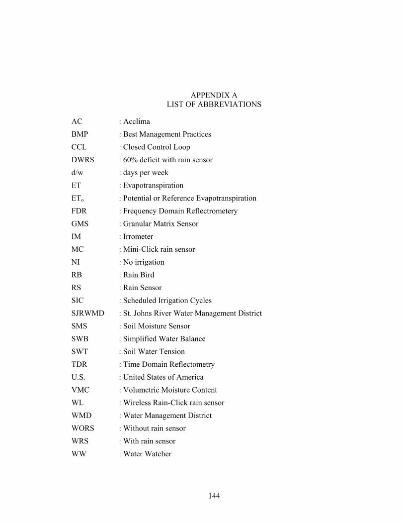
144
APPENDIX A LIST OF ABBREVIATIONS
AC : Acclima BMP : Best Management Practices CCL : Closed Control Loop DWRS : 60% deficit with rain sensor d/w : days per week ET : Evapotranspiration ETo : Potential or Reference Evapotranspiration FDR : Frequency Domain Reflectrometery GMS : Granular Matrix Sensor IM : Irrometer MC : Mini-Click rain sensor NI : No irrigation RB : Rain Bird RS : Rain Sensor SIC : Scheduled Irrigation Cycles SJRWMD : St. Johns River Water Management District SMS : Soil Moisture Sensor SWB : Simplified Water Balance SWT : Soil Water Tension TDR : Time Domain Reflectometry U.S. : United States of America VMC : Volumetric Moisture Content WL : Wireless Rain-Click rain sensor WMD : Water Management District WORS : Without rain sensor WRS : With rain sensor WW : Water Watcher
145
APPENDIX B STATISTICAL ANALYSES
The following are the SAS codes and the output text files for the statistical analyses
performed.
DRY-WET CODES
options nodate nonumber center formdlim="*"linesize=85; data sms; input plot$ rep$ dry wet; cards; /* Data is inputted here */ ; data sms; set sms; proc glm data=sms; title 'Dry'; class plot; model dry = plot /ss3; means plot/duncan; run; data sms; set sms; proc glm data=sms; title 'Wet'; class plot; model wet = plot /ss3; means plot/duncan; run;
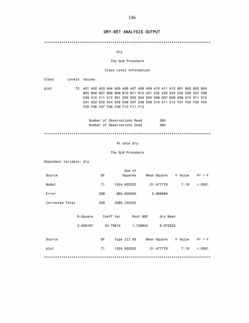
146
DRY-WET ANALYSIS OUTPUT
************************************************************************************* Dry The GLM Procedure Class Level Information Class Levels Values plot 72 A01 A02 A03 A04 A05 A06 A07 A08 A09 A10 A11 A12 B01 B02 B03 B04 B05 B06 B07 B08 B09 B10 B11 B12 C01 C02 C03 C04 C05 C06 C07 C08 C09 C10 C11 C12 D01 D02 D03 D04 D05 D06 D07 D08 D09 D10 D11 D12 E01 E02 E03 E04 E05 E06 E07 E08 E09 E10 E11 E12 F01 F02 F03 F04 F05 F06 F07 F08 F09 F10 F11 F12 Number of Observations Read 360 Number of Observations Used 360 ************************************************************************************* At once Dry The GLM Procedure Dependent Variable: dry Sum of Source DF Squares Mean Square F Value Pr > F Model 71 1524.922222 21.477778 7.19 <.0001 Error 288 860.800000 2.988889 Corrected Total 359 2385.722222 R-Square Coeff Var Root MSE dry Mean 0.639187 24.79612 1.728840 6.972222 Source DF Type III SS Mean Square F Value Pr > F plot 71 1524.922222 21.477778 7.19 <.0001 *************************************************************************************
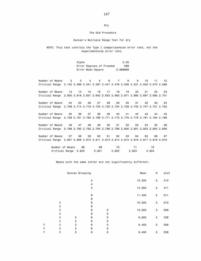
147
Dry The GLM Procedure Duncan's Multiple Range Test for dry NOTE: This test controls the Type I comparisonwise error rate, not the experimentwise error rate. Alpha 0.05 Error Degrees of Freedom 288 Error Mean Square 2.988889 Number of Means 2 3 4 5 6 7 8 9 10 11 12 Critical Range 2.152 2.266 2.341 2.397 2.441 2.476 2.506 2.531 2.553 2.572 2.589 Number of Means 13 14 15 16 17 18 19 20 21 22 23 Critical Range 2.605 2.618 2.631 2.642 2.653 2.663 2.671 2.680 2.687 2.695 2.701 Number of Means 24 25 26 27 28 29 30 31 32 33 34 Critical Range 2.708 2.714 2.719 2.725 2.730 2.734 2.739 2.743 2.747 2.751 2.755 Number of Means 35 36 37 38 39 40 41 42 43 44 45 Critical Range 2.758 2.761 2.765 2.768 2.771 2.773 2.776 2.779 2.781 2.784 2.786 Number of Means 46 47 48 49 50 51 52 53 54 55 56 Critical Range 2.788 2.790 2.792 2.794 2.796 2.798 2.800 2.801 2.803 2.804 2.806 Number of Means 57 58 59 60 61 62 63 64 65 66 67 Critical Range 2.807 2.809 2.810 2.811 2.813 2.814 2.815 2.816 2.817 2.818 2.819 Number of Means 68 69 70 71 72 Critical Range 2.820 2.821 2.822 2.823 2.824 Means with the same letter are not significantly different. Duncan Grouping Mean N plot A 15.200 5 A12 A A 14.000 5 A11 B 11.400 5 D11 B C B 10.200 5 D10 C B C B D 10.000 5 D09 C B D C E B D 9.600 5 C08 C E B D F C E B D 9.400 5 D06 F C E B D F C E B D 9.400 5 E08
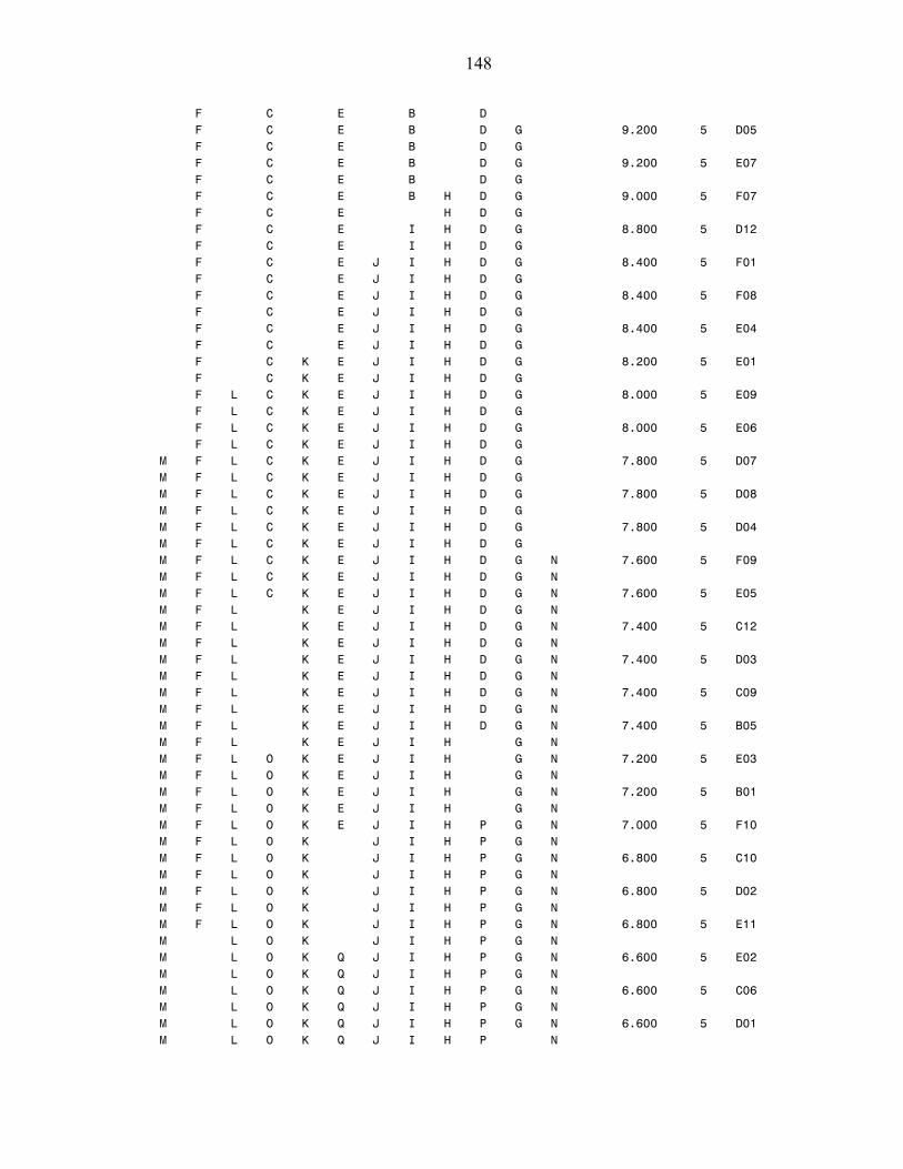
148
F C E B D F C E B D G 9.200 5 D05 F C E B D G F C E B D G 9.200 5 E07 F C E B D G F C E B H D G 9.000 5 F07 F C E H D G F C E I H D G 8.800 5 D12 F C E I H D G F C E J I H D G 8.400 5 F01 F C E J I H D G F C E J I H D G 8.400 5 F08 F C E J I H D G F C E J I H D G 8.400 5 E04 F C E J I H D G F C K E J I H D G 8.200 5 E01 F C K E J I H D G F L C K E J I H D G 8.000 5 E09 F L C K E J I H D G F L C K E J I H D G 8.000 5 E06 F L C K E J I H D G M F L C K E J I H D G 7.800 5 D07 M F L C K E J I H D G M F L C K E J I H D G 7.800 5 D08 M F L C K E J I H D G M F L C K E J I H D G 7.800 5 D04 M F L C K E J I H D G M F L C K E J I H D G N 7.600 5 F09 M F L C K E J I H D G N M F L C K E J I H D G N 7.600 5 E05 M F L K E J I H D G N M F L K E J I H D G N 7.400 5 C12 M F L K E J I H D G N M F L K E J I H D G N 7.400 5 D03 M F L K E J I H D G N M F L K E J I H D G N 7.400 5 C09 M F L K E J I H D G N M F L K E J I H D G N 7.400 5 B05 M F L K E J I H G N M F L O K E J I H G N 7.200 5 E03 M F L O K E J I H G N M F L O K E J I H G N 7.200 5 B01 M F L O K E J I H G N M F L O K E J I H P G N 7.000 5 F10 M F L O K J I H P G N M F L O K J I H P G N 6.800 5 C10 M F L O K J I H P G N M F L O K J I H P G N 6.800 5 D02 M F L O K J I H P G N M F L O K J I H P G N 6.800 5 E11 M L O K J I H P G N M L O K Q J I H P G N 6.600 5 E02 M L O K Q J I H P G N M L O K Q J I H P G N 6.600 5 C06 M L O K Q J I H P G N M L O K Q J I H P G N 6.600 5 D01 M L O K Q J I H P N
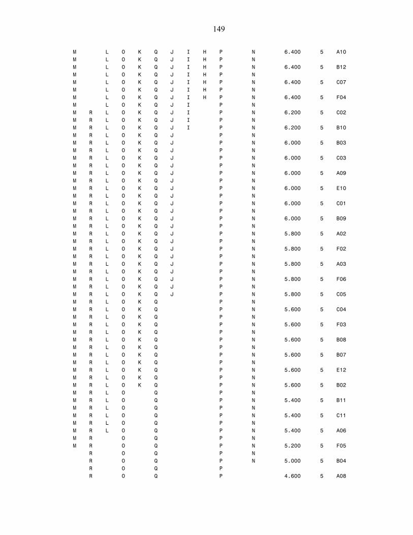
149
M L O K Q J I H P N 6.400 5 A10 M L O K Q J I H P N M L O K Q J I H P N 6.400 5 B12 M L O K Q J I H P N M L O K Q J I H P N 6.400 5 C07 M L O K Q J I H P N M L O K Q J I H P N 6.400 5 F04 M L O K Q J I P N M R L O K Q J I P N 6.200 5 C02 M R L O K Q J I P N M R L O K Q J I P N 6.200 5 B10 M R L O K Q J P N M R L O K Q J P N 6.000 5 B03 M R L O K Q J P N M R L O K Q J P N 6.000 5 C03 M R L O K Q J P N M R L O K Q J P N 6.000 5 A09 M R L O K Q J P N M R L O K Q J P N 6.000 5 E10 M R L O K Q J P N M R L O K Q J P N 6.000 5 C01 M R L O K Q J P N M R L O K Q J P N 6.000 5 B09 M R L O K Q J P N M R L O K Q J P N 5.800 5 A02 M R L O K Q J P N M R L O K Q J P N 5.800 5 F02 M R L O K Q J P N M R L O K Q J P N 5.800 5 A03 M R L O K Q J P N M R L O K Q J P N 5.800 5 F06 M R L O K Q J P N M R L O K Q J P N 5.800 5 C05 M R L O K Q P N M R L O K Q P N 5.600 5 C04 M R L O K Q P N M R L O K Q P N 5.600 5 F03 M R L O K Q P N M R L O K Q P N 5.600 5 B08 M R L O K Q P N M R L O K Q P N 5.600 5 B07 M R L O K Q P N M R L O K Q P N 5.600 5 E12 M R L O K Q P N M R L O K Q P N 5.600 5 B02 M R L O Q P N M R L O Q P N 5.400 5 B11 M R L O Q P N M R L O Q P N 5.400 5 C11 M R L O Q P N M R L O Q P N 5.400 5 A06 M R O Q P N M R O Q P N 5.200 5 F05 R O Q P N R O Q P N 5.000 5 B04 R O Q P R O Q P 4.600 5 A08

150
R O Q P R O Q P 4.600 5 B06 R Q P R Q P 4.400 5 A01 R Q P R Q P 4.400 5 A07 R Q P R Q P 4.400 5 A04 R Q P R Q P 4.400 5 F12 R Q R Q 4.000 5 F11 R R 3.600 5 A05 ************************************************************************************* Wet The GLM Procedure Class Level Information Class Levels Values plot 72 A01 A02 A03 A04 A05 A06 A07 A08 A09 A10 A11 A12 B01 B02 B03 B04 B05 B06 B07 B08 B09 B10 B11 B12 C01 C02 C03 C04 C05 C06 C07 C08 C09 C10 C11 C12 D01 D02 D03 D04 D05 D06 D07 D08 D09 D10 D11 D12 E01 E02 E03 E04 E05 E06 E07 E08 E09 E10 E11 E12 F01 F02 F03 F04 F05 F06 F07 F08 F09 F10 F11 F12 Number of Observations Read 360 Number of Observations Used 360 *************************************************************************************
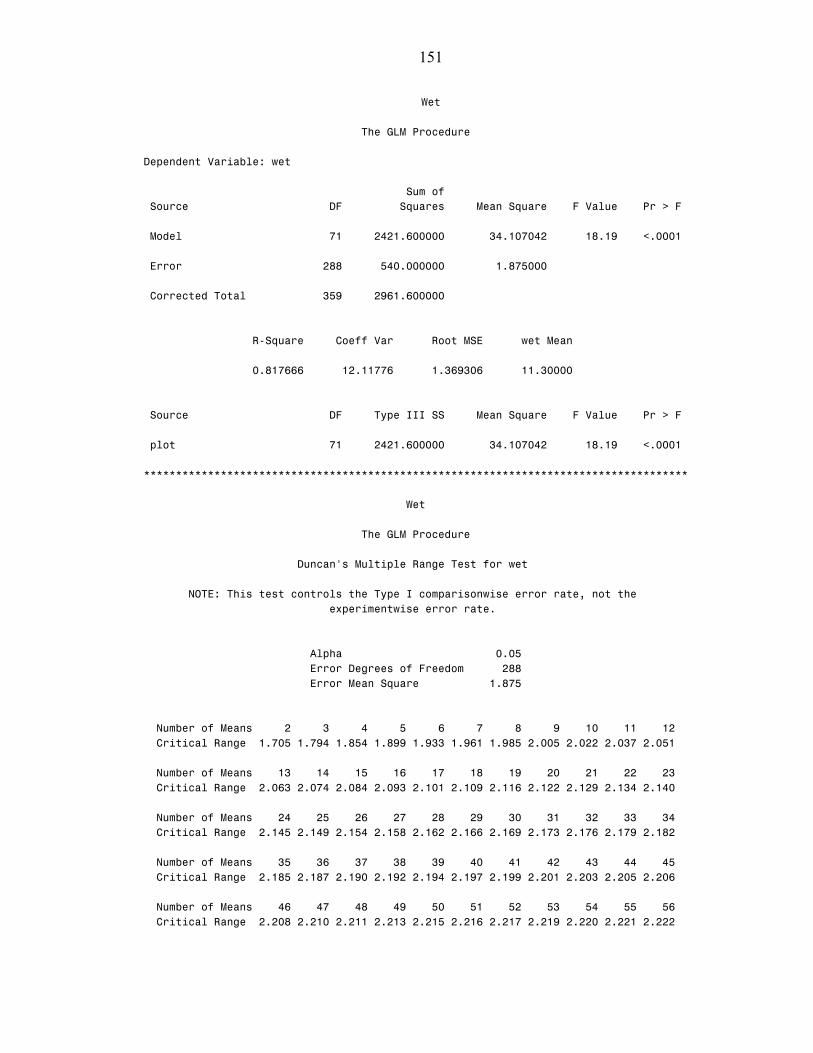
151
Wet The GLM Procedure Dependent Variable: wet Sum of Source DF Squares Mean Square F Value Pr > F Model 71 2421.600000 34.107042 18.19 <.0001 Error 288 540.000000 1.875000 Corrected Total 359 2961.600000 R-Square Coeff Var Root MSE wet Mean 0.817666 12.11776 1.369306 11.30000 Source DF Type III SS Mean Square F Value Pr > F plot 71 2421.600000 34.107042 18.19 <.0001 ************************************************************************************* Wet The GLM Procedure Duncan's Multiple Range Test for wet NOTE: This test controls the Type I comparisonwise error rate, not the experimentwise error rate. Alpha 0.05 Error Degrees of Freedom 288 Error Mean Square 1.875 Number of Means 2 3 4 5 6 7 8 9 10 11 12 Critical Range 1.705 1.794 1.854 1.899 1.933 1.961 1.985 2.005 2.022 2.037 2.051 Number of Means 13 14 15 16 17 18 19 20 21 22 23 Critical Range 2.063 2.074 2.084 2.093 2.101 2.109 2.116 2.122 2.129 2.134 2.140 Number of Means 24 25 26 27 28 29 30 31 32 33 34 Critical Range 2.145 2.149 2.154 2.158 2.162 2.166 2.169 2.173 2.176 2.179 2.182 Number of Means 35 36 37 38 39 40 41 42 43 44 45 Critical Range 2.185 2.187 2.190 2.192 2.194 2.197 2.199 2.201 2.203 2.205 2.206 Number of Means 46 47 48 49 50 51 52 53 54 55 56 Critical Range 2.208 2.210 2.211 2.213 2.215 2.216 2.217 2.219 2.220 2.221 2.222
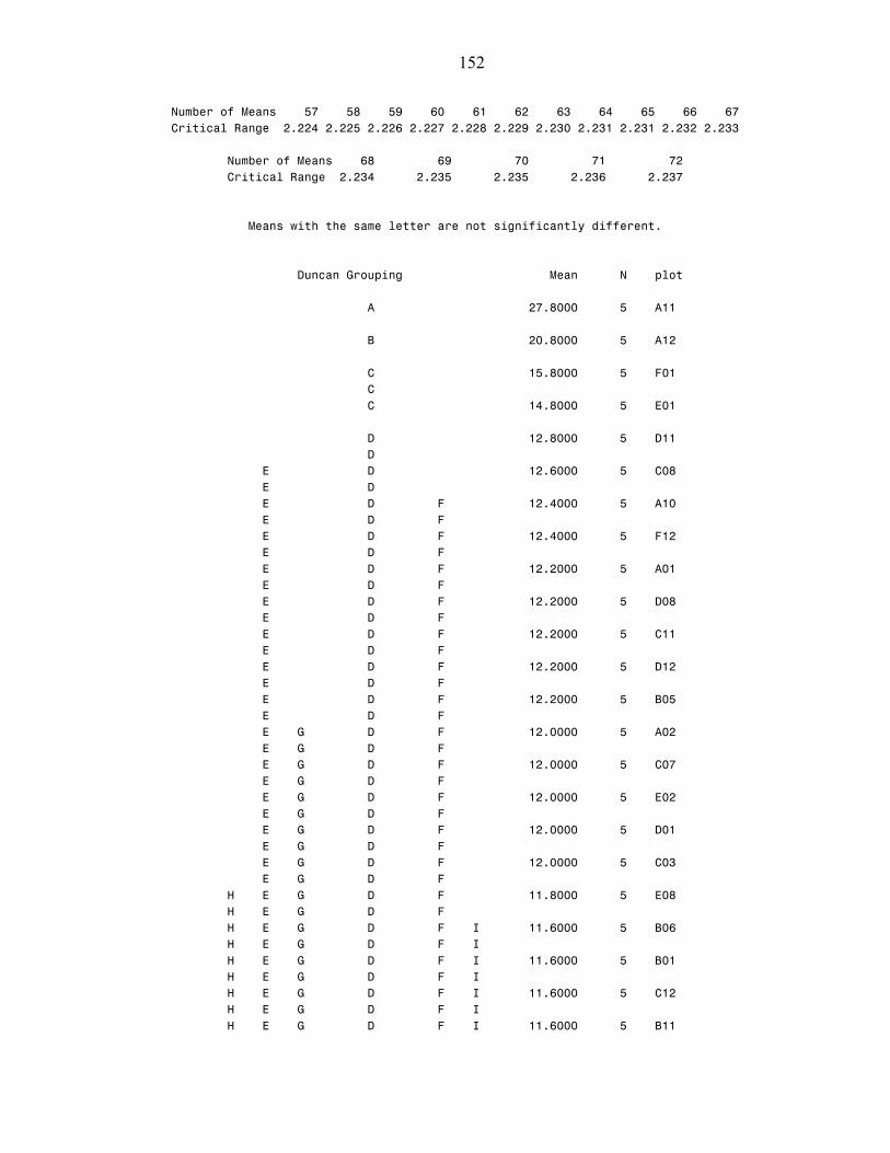
152
Number of Means 57 58 59 60 61 62 63 64 65 66 67 Critical Range 2.224 2.225 2.226 2.227 2.228 2.229 2.230 2.231 2.231 2.232 2.233 Number of Means 68 69 70 71 72 Critical Range 2.234 2.235 2.235 2.236 2.237 Means with the same letter are not significantly different. Duncan Grouping Mean N plot A 27.8000 5 A11 B 20.8000 5 A12 C 15.8000 5 F01 C C 14.8000 5 E01 D 12.8000 5 D11 D E D 12.6000 5 C08 E D E D F 12.4000 5 A10 E D F E D F 12.4000 5 F12 E D F E D F 12.2000 5 A01 E D F E D F 12.2000 5 D08 E D F E D F 12.2000 5 C11 E D F E D F 12.2000 5 D12 E D F E D F 12.2000 5 B05 E D F E G D F 12.0000 5 A02 E G D F E G D F 12.0000 5 C07 E G D F E G D F 12.0000 5 E02 E G D F E G D F 12.0000 5 D01 E G D F E G D F 12.0000 5 C03 E G D F H E G D F 11.8000 5 E08 H E G D F H E G D F I 11.6000 5 B06 H E G D F I H E G D F I 11.6000 5 B01 H E G D F I H E G D F I 11.6000 5 C12 H E G D F I H E G D F I 11.6000 5 B11

153
H E G D F I H E G D J F I 11.4000 5 A08 H E G D J F I H E G D J F I 11.4000 5 A09 H E G D J F I H E G D J F I 11.4000 5 D09 H E G D J F I H E G D J F I 11.2000 5 D02 H E G D J F I H E G D J F I 11.2000 5 B02 H E G D J F I H E G D J F I 11.2000 5 F07 H E G D J F I H E G D J F I 11.2000 5 C01 H E G D J F I H E G D J F I 11.2000 5 B09 H E G D J F I H E G D J F I 11.0000 5 E12 H E G D J F I H E G D J F I 11.0000 5 B12 H E G D J F I H E G D J F I 11.0000 5 E07 H E G D J F I H E G D J F I 11.0000 5 D07 H E G D J F I H E G D J F I 11.0000 5 C09 H E G D J F I H E G K D J F I 10.8000 5 E10 H E G K D J F I H E G K D J F I 10.8000 5 D06 H E G K D J F I H E G K D J F I 10.8000 5 E03 H E G K D J F I H E G K D J F I 10.8000 5 E11 H E G K D J F I H E G K D J F I 10.8000 5 F09 H E G K J F I H E G K L J F I 10.6000 5 A06 H E G K L J F I H E G K L J F I 10.6000 5 F02 H E G K L J F I H E G K L J F I 10.6000 5 B08 H E G K L J F I H E G K L J F I 10.6000 5 F08 H E G K L J F I H E G K L J F I 10.4000 5 D10 H E G K L J F I H E G K L J F I 10.4000 5 D03 H E G K L J F I H E G K L J F I 10.4000 5 C10 H E G K L J F I H E G K L J F I 10.4000 5 E09 H E G K L J F I H E G K L J F I 10.4000 5 E05 H E G K L J F I H E G K L J F I 10.4000 5 C05 H G K L J F I
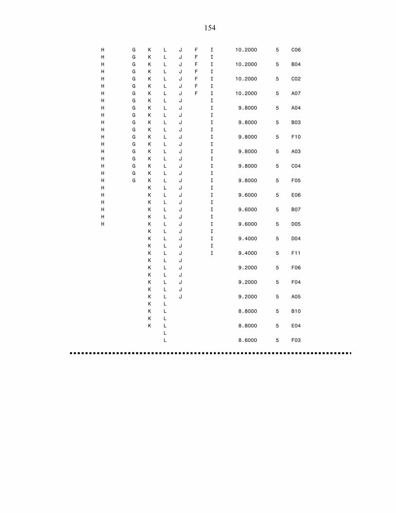
154
H G K L J F I 10.2000 5 C06 H G K L J F I H G K L J F I 10.2000 5 B04 H G K L J F I H G K L J F I 10.2000 5 C02 H G K L J F I H G K L J F I 10.2000 5 A07 H G K L J I H G K L J I 9.8000 5 A04 H G K L J I H G K L J I 9.8000 5 B03 H G K L J I H G K L J I 9.8000 5 F10 H G K L J I H G K L J I 9.8000 5 A03 H G K L J I H G K L J I 9.8000 5 C04 H G K L J I H G K L J I 9.8000 5 F05 H K L J I H K L J I 9.6000 5 E06 H K L J I H K L J I 9.6000 5 B07 H K L J I H K L J I 9.6000 5 D05 K L J I K L J I 9.4000 5 D04 K L J I K L J I 9.4000 5 F11 K L J K L J 9.2000 5 F06 K L J K L J 9.2000 5 F04 K L J K L J 9.2000 5 A05 K L K L 8.8000 5 B10 K L K L 8.8000 5 E04 L L 8.6000 5 F03
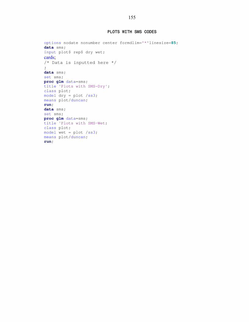
155
PLOTS WITH SMS CODES
options nodate nonumber center formdlim="*"linesize=85; data sms; input plot$ rep$ dry wet; cards; /* Data is inputted here */ ; data sms; set sms; proc glm data=sms; title 'Plots with SMS-Dry'; class plot; model dry = plot /ss3; means plot/duncan; run; data sms; set sms; proc glm data=sms; title 'Plots with SMS-Wet; class plot; model wet = plot /ss3; means plot/duncan; run;
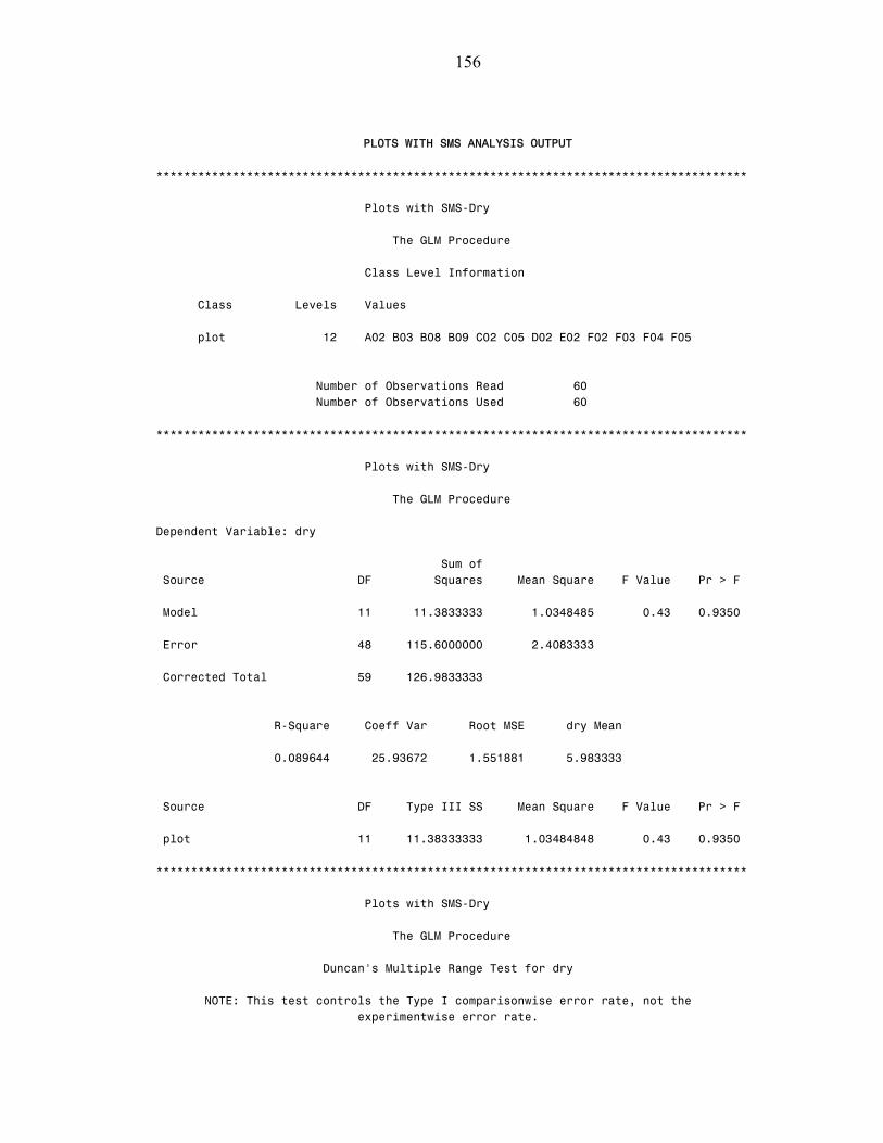
156
PLOTS WITH SMS ANALYSIS OUTPUT
************************************************************************************* Plots with SMS-Dry The GLM Procedure Class Level Information Class Levels Values plot 12 A02 B03 B08 B09 C02 C05 D02 E02 F02 F03 F04 F05 Number of Observations Read 60 Number of Observations Used 60 ************************************************************************************* Plots with SMS-Dry The GLM Procedure Dependent Variable: dry Sum of Source DF Squares Mean Square F Value Pr > F Model 11 11.3833333 1.0348485 0.43 0.9350 Error 48 115.6000000 2.4083333 Corrected Total 59 126.9833333 R-Square Coeff Var Root MSE dry Mean 0.089644 25.93672 1.551881 5.983333 Source DF Type III SS Mean Square F Value Pr > F plot 11 11.38333333 1.03484848 0.43 0.9350 ************************************************************************************* Plots with SMS-Dry The GLM Procedure Duncan's Multiple Range Test for dry NOTE: This test controls the Type I comparisonwise error rate, not the experimentwise error rate.
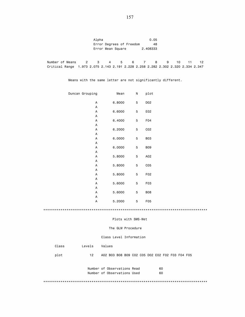
157
Alpha 0.05 Error Degrees of Freedom 48 Error Mean Square 2.408333 Number of Means 2 3 4 5 6 7 8 9 10 11 12 Critical Range 1.973 2.075 2.143 2.191 2.228 2.258 2.282 2.302 2.320 2.334 2.347 Means with the same letter are not significantly different. Duncan Grouping Mean N plot A 6.8000 5 D02 A A 6.6000 5 E02 A A 6.4000 5 F04 A A 6.2000 5 C02 A A 6.0000 5 B03 A A 6.0000 5 B09 A A 5.8000 5 A02 A A 5.8000 5 C05 A A 5.8000 5 F02 A A 5.6000 5 F03 A A 5.6000 5 B08 A A 5.2000 5 F05 *************************************************************************************
Plots with SMS-Wet The GLM Procedure Class Level Information Class Levels Values plot 12 A02 B03 B08 B09 C02 C05 D02 E02 F02 F03 F04 F05 Number of Observations Read 60 Number of Observations Used 60 *************************************************************************************

158
Plots with SMS-Wet The GLM Procedure Dependent Variable: wet Sum of Source DF Squares Mean Square F Value Pr > F Model 11 59.3333333 5.3939394 5.22 <.0001 Error 48 49.6000000 1.0333333 Corrected Total 59 108.9333333 R-Square Coeff Var Root MSE wet Mean 0.544676 9.712070 1.016530 10.46667 Source DF Type III SS Mean Square F Value Pr > F plot 11 59.33333333 5.39393939 5.22 <.0001 *************************************************************************************
Plots with SMS-Wet The GLM Procedure Duncan's Multiple Range Test for wet NOTE: This test controls the Type I comparisonwise error rate, not the experimentwise error rate. Alpha 0.05 Error Degrees of Freedom 48 Error Mean Square 1.033333 Number of Means 2 3 4 5 6 7 8 9 10 11 12 Critical Range 1.293 1.360 1.403 1.435 1.460 1.479 1.495 1.508 1.519 1.529 1.537 Means with the same letter are not significantly different. Duncan Grouping Mean N plot A 12.0000 5 A02 A A 12.0000 5 E02 A
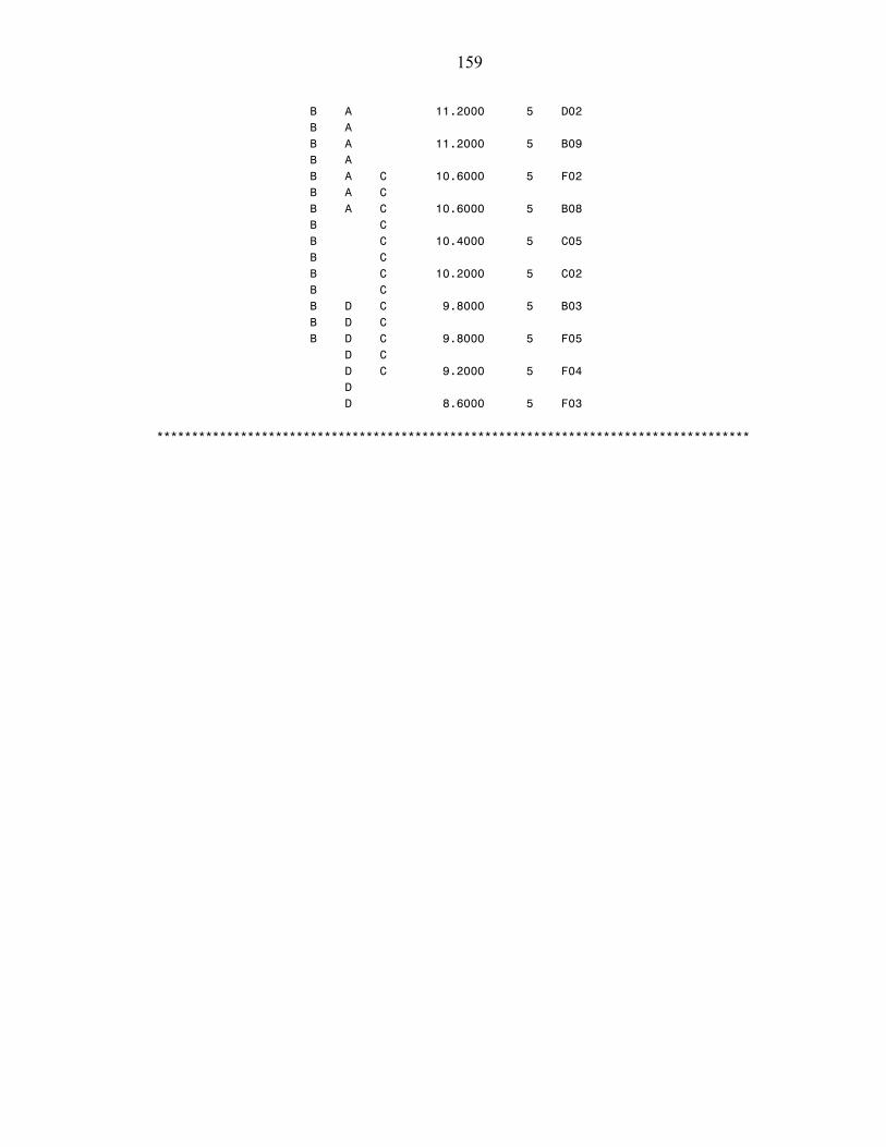
159
B A 11.2000 5 D02 B A B A 11.2000 5 B09 B A B A C 10.6000 5 F02 B A C B A C 10.6000 5 B08 B C B C 10.4000 5 C05 B C B C 10.2000 5 C02 B C B D C 9.8000 5 B03 B D C B D C 9.8000 5 F05 D C D C 9.2000 5 F04 D D 8.6000 5 F03 *************************************************************************************
160
CUMULATIVE IRRIGATION DEPTH, YEAR 2004
options nodate nonumber center formdlim="*"linesize=85; data sms; input tmt$ day$ brand$ type$ based$ timeb$ mm; cards; /* Data is inputted here */ ; data sms2; set sms(where=(type = 'sms')); proc glm data=sms2; title 'TOTAL Cumulative mm (21 July 2004 – 14 Dec 2004)'; class brand day; model mm = day brand day(brand) /ss3; test h=brand e=day(brand); means day/duncan; means brand/duncan; means brand/duncan e=day(brand); run; proc glm data=sms2; title 'Comparison of Interaction'; class brand day; model mm = brand*day /ss3; means brand*day/duncan; run; data sms3; set sms(where=(day = '1')); proc glm data=sms3; title 'Cumulative mm-- Once per Week'; class brand ; model mm = brand/ss3; means brand/duncan; run; data sms3; set sms(where=(day = '2')); proc glm data=sms3; title 'Cumulative mm-- Twice per Week'; class brand ; model mm = brand/ss3; means brand/duncan; run; data sms3; set sms(where=(day = '7')); proc glm data=sms3; title 'Cumulative mm-- Everyday'; class brand ; model mm = brand/ss3; means brand/duncan; run; data sms; set sms; proc glm data=sms; title 'Comparison of Time-based treatments'; class timeb; model mm = timeb /ss3;
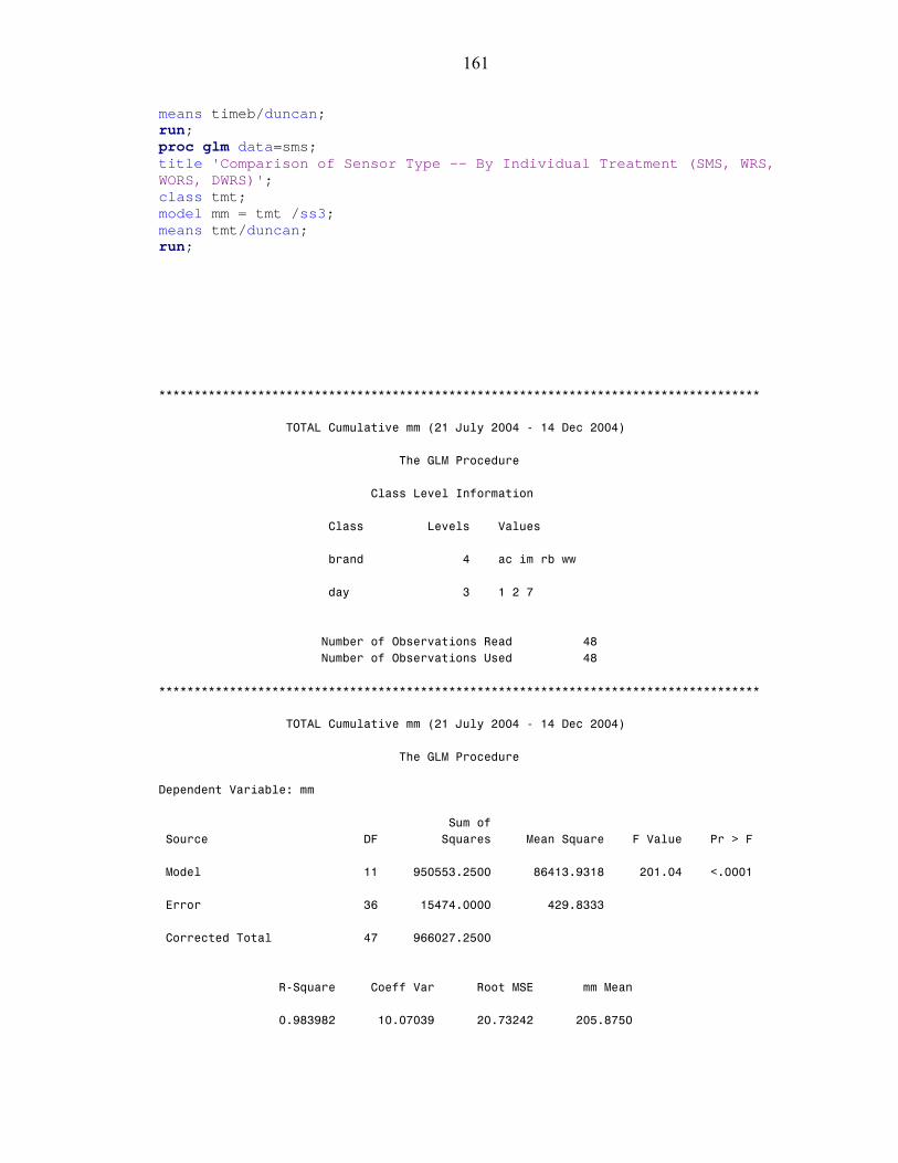
161
means timeb/duncan; run; proc glm data=sms; title 'Comparison of Sensor Type -- By Individual Treatment (SMS, WRS, WORS, DWRS)'; class tmt; model mm = tmt /ss3; means tmt/duncan; run; ************************************************************************************* TOTAL Cumulative mm (21 July 2004 - 14 Dec 2004) The GLM Procedure Class Level Information Class Levels Values brand 4 ac im rb ww day 3 1 2 7 Number of Observations Read 48 Number of Observations Used 48 ************************************************************************************* TOTAL Cumulative mm (21 July 2004 - 14 Dec 2004) The GLM Procedure Dependent Variable: mm Sum of Source DF Squares Mean Square F Value Pr > F Model 11 950553.2500 86413.9318 201.04 <.0001 Error 36 15474.0000 429.8333 Corrected Total 47 966027.2500 R-Square Coeff Var Root MSE mm Mean 0.983982 10.07039 20.73242 205.8750
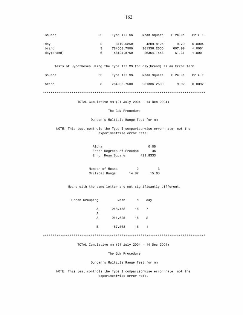
162
Source DF Type III SS Mean Square F Value Pr > F day 2 8419.6250 4209.8125 9.79 0.0004 brand 3 784008.7500 261336.2500 607.99 <.0001 day(brand) 6 158124.8750 26354.1458 61.31 <.0001 Tests of Hypotheses Using the Type III MS for day(brand) as an Error Term Source DF Type III SS Mean Square F Value Pr > F brand 3 784008.7500 261336.2500 9.92 0.0097 ************************************************************************************* TOTAL Cumulative mm (21 July 2004 - 14 Dec 2004) The GLM Procedure Duncan's Multiple Range Test for mm NOTE: This test controls the Type I comparisonwise error rate, not the experimentwise error rate. Alpha 0.05 Error Degrees of Freedom 36 Error Mean Square 429.8333 Number of Means 2 3 Critical Range 14.87 15.63 Means with the same letter are not significantly different. Duncan Grouping Mean N day A 218.438 16 7 A A 211.625 16 2 B 187.563 16 1 ************************************************************************************* TOTAL Cumulative mm (21 July 2004 - 14 Dec 2004) The GLM Procedure Duncan's Multiple Range Test for mm NOTE: This test controls the Type I comparisonwise error rate, not the experimentwise error rate.
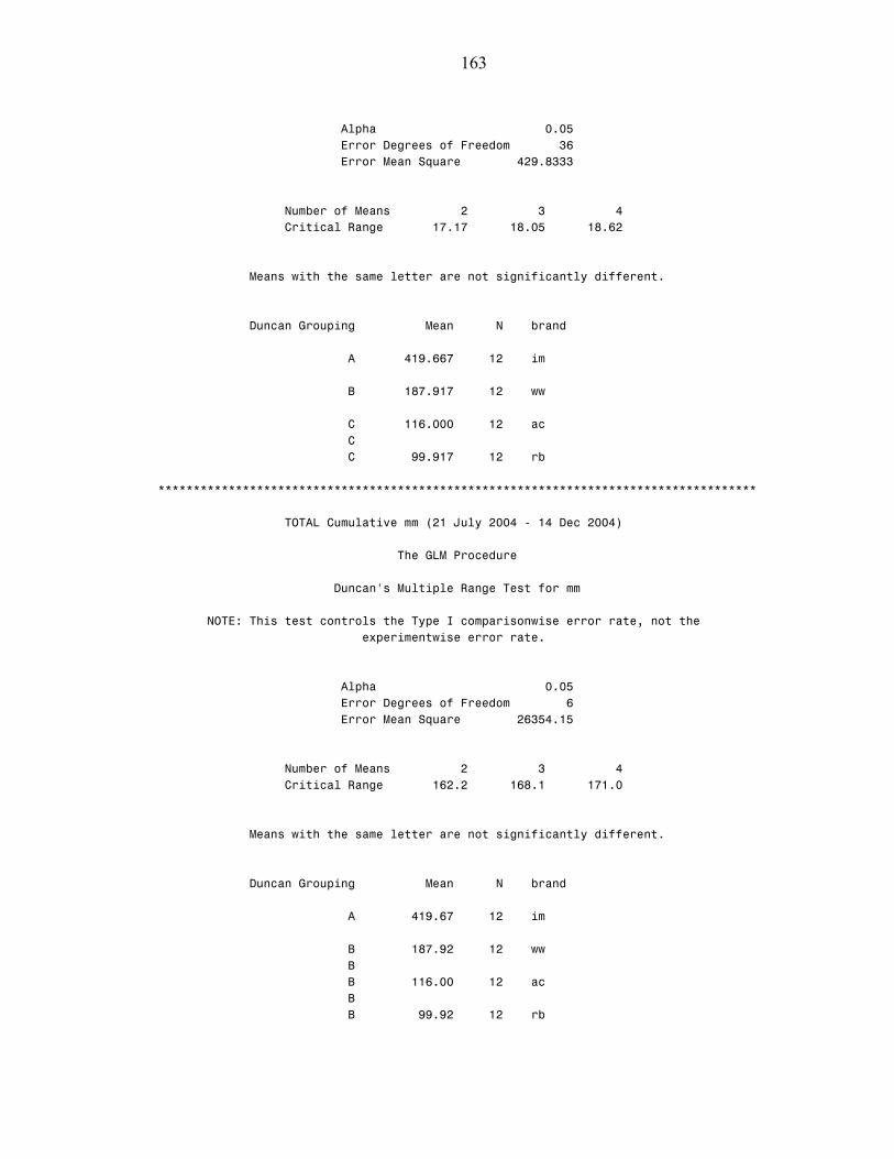
163
Alpha 0.05 Error Degrees of Freedom 36 Error Mean Square 429.8333 Number of Means 2 3 4 Critical Range 17.17 18.05 18.62 Means with the same letter are not significantly different. Duncan Grouping Mean N brand A 419.667 12 im B 187.917 12 ww C 116.000 12 ac C C 99.917 12 rb ************************************************************************************* TOTAL Cumulative mm (21 July 2004 - 14 Dec 2004) The GLM Procedure Duncan's Multiple Range Test for mm NOTE: This test controls the Type I comparisonwise error rate, not the experimentwise error rate. Alpha 0.05 Error Degrees of Freedom 6 Error Mean Square 26354.15 Number of Means 2 3 4 Critical Range 162.2 168.1 171.0 Means with the same letter are not significantly different. Duncan Grouping Mean N brand A 419.67 12 im B 187.92 12 ww B B 116.00 12 ac B B 99.92 12 rb

164
************************************************************************************* Comparison of Interaction The GLM Procedure Class Level Information Class Levels Values brand 4 ac im rb ww day 3 1 2 7 Number of Observations Read 48 Number of Observations Used 48 ************************************************************************************* Comparison of Interaction The GLM Procedure Dependent Variable: mm Sum of Source DF Squares Mean Square F Value Pr > F Model 11 950553.2500 86413.9318 201.04 <.0001 Error 36 15474.0000 429.8333 Corrected Total 47 966027.2500 R-Square Coeff Var Root MSE mm Mean 0.983982 10.07039 20.73242 205.8750 Source DF Type III SS Mean Square F Value Pr > F brand*day 11 950553.2500 86413.9318 201.04 <.0001 ************************************************************************************* Comparison of Interaction The GLM Procedure Level of Level of --------------mm------------- brand day N Mean Std Dev ac 1 4 95.250000 2.0615528 ac 2 4 196.000000 8.7939373 ac 7 4 56.750000 2.6299556
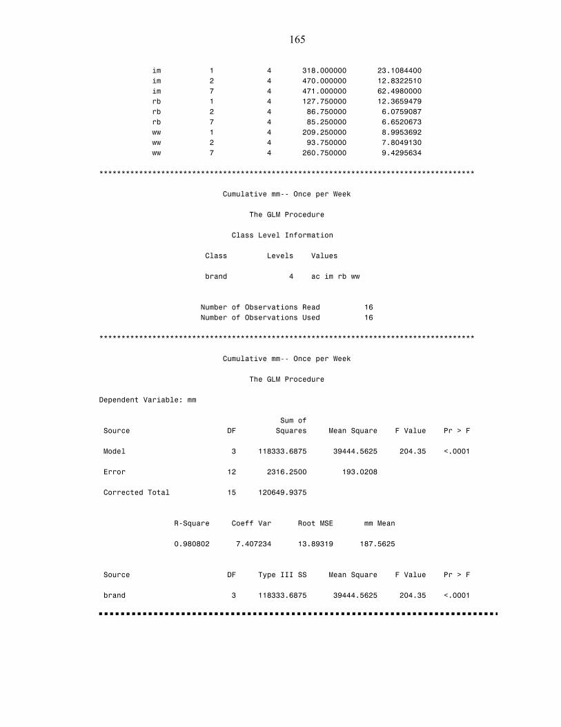
165
im 1 4 318.000000 23.1084400 im 2 4 470.000000 12.8322510 im 7 4 471.000000 62.4980000 rb 1 4 127.750000 12.3659479 rb 2 4 86.750000 6.0759087 rb 7 4 85.250000 6.6520673 ww 1 4 209.250000 8.9953692 ww 2 4 93.750000 7.8049130 ww 7 4 260.750000 9.4295634 ************************************************************************************* Cumulative mm-- Once per Week The GLM Procedure Class Level Information Class Levels Values brand 4 ac im rb ww Number of Observations Read 16 Number of Observations Used 16 ************************************************************************************* Cumulative mm-- Once per Week The GLM Procedure Dependent Variable: mm Sum of Source DF Squares Mean Square F Value Pr > F Model 3 118333.6875 39444.5625 204.35 <.0001 Error 12 2316.2500 193.0208 Corrected Total 15 120649.9375 R-Square Coeff Var Root MSE mm Mean 0.980802 7.407234 13.89319 187.5625 Source DF Type III SS Mean Square F Value Pr > F brand 3 118333.6875 39444.5625 204.35 <.0001
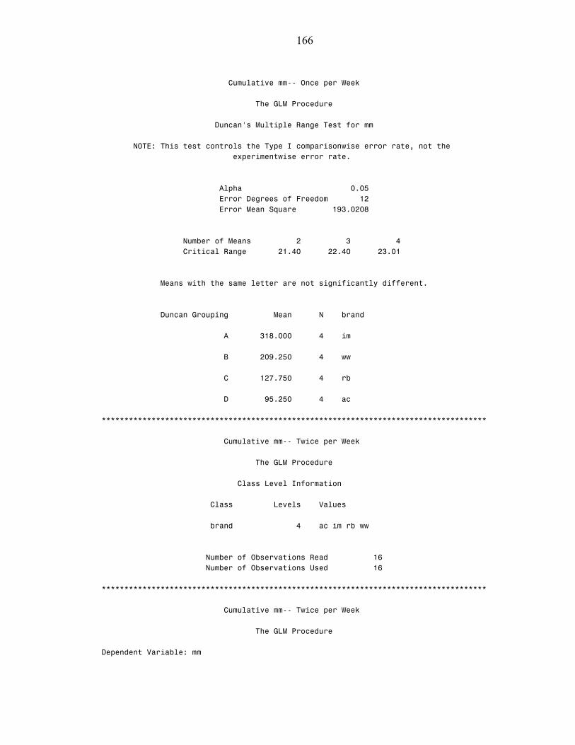
166
Cumulative mm-- Once per Week The GLM Procedure Duncan's Multiple Range Test for mm NOTE: This test controls the Type I comparisonwise error rate, not the experimentwise error rate. Alpha 0.05 Error Degrees of Freedom 12 Error Mean Square 193.0208 Number of Means 2 3 4 Critical Range 21.40 22.40 23.01 Means with the same letter are not significantly different. Duncan Grouping Mean N brand A 318.000 4 im B 209.250 4 ww C 127.750 4 rb D 95.250 4 ac ************************************************************************************* Cumulative mm-- Twice per Week The GLM Procedure Class Level Information Class Levels Values brand 4 ac im rb ww Number of Observations Read 16 Number of Observations Used 16 ************************************************************************************* Cumulative mm-- Twice per Week The GLM Procedure Dependent Variable: mm
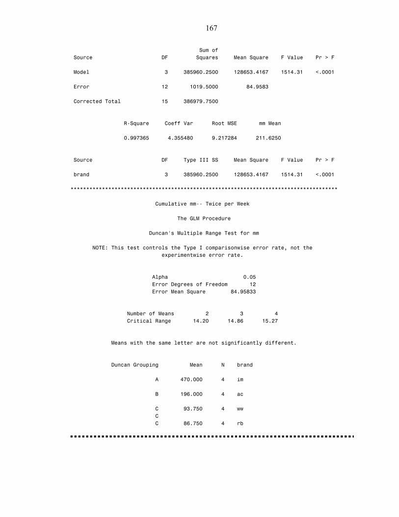
167
Sum of Source DF Squares Mean Square F Value Pr > F Model 3 385960.2500 128653.4167 1514.31 <.0001 Error 12 1019.5000 84.9583 Corrected Total 15 386979.7500 R-Square Coeff Var Root MSE mm Mean 0.997365 4.355480 9.217284 211.6250 Source DF Type III SS Mean Square F Value Pr > F brand 3 385960.2500 128653.4167 1514.31 <.0001 ************************************************************************************* Cumulative mm-- Twice per Week The GLM Procedure Duncan's Multiple Range Test for mm NOTE: This test controls the Type I comparisonwise error rate, not the experimentwise error rate. Alpha 0.05 Error Degrees of Freedom 12 Error Mean Square 84.95833 Number of Means 2 3 4 Critical Range 14.20 14.86 15.27 Means with the same letter are not significantly different. Duncan Grouping Mean N brand A 470.000 4 im B 196.000 4 ac C 93.750 4 ww C C 86.750 4 rb
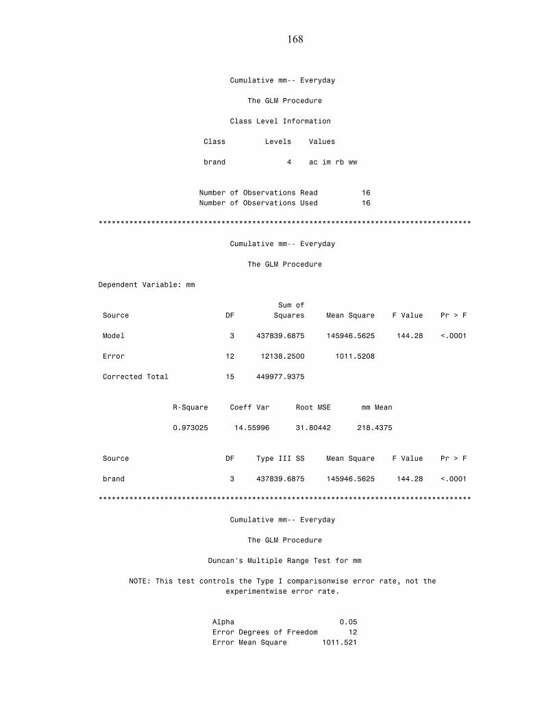
168
Cumulative mm-- Everyday The GLM Procedure Class Level Information Class Levels Values brand 4 ac im rb ww Number of Observations Read 16 Number of Observations Used 16 ************************************************************************************* Cumulative mm-- Everyday The GLM Procedure Dependent Variable: mm Sum of Source DF Squares Mean Square F Value Pr > F Model 3 437839.6875 145946.5625 144.28 <.0001 Error 12 12138.2500 1011.5208 Corrected Total 15 449977.9375 R-Square Coeff Var Root MSE mm Mean 0.973025 14.55996 31.80442 218.4375 Source DF Type III SS Mean Square F Value Pr > F brand 3 437839.6875 145946.5625 144.28 <.0001 ************************************************************************************* Cumulative mm-- Everyday The GLM Procedure Duncan's Multiple Range Test for mm NOTE: This test controls the Type I comparisonwise error rate, not the experimentwise error rate. Alpha 0.05 Error Degrees of Freedom 12 Error Mean Square 1011.521
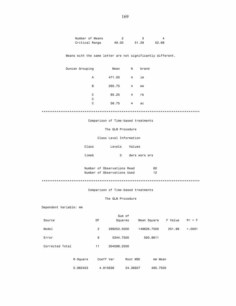
169
Number of Means 2 3 4 Critical Range 49.00 51.29 52.68 Means with the same letter are not significantly different. Duncan Grouping Mean N brand A 471.00 4 im B 260.75 4 ww C 85.25 4 rb C C 56.75 4 ac ************************************************************************************* Comparison of Time-based treatments The GLM Procedure Class Level Information Class Levels Values timeb 3 dwrs wors wrs Number of Observations Read 60 Number of Observations Used 12 ************************************************************************************* Comparison of Time-based treatments The GLM Procedure Dependent Variable: mm Sum of Source DF Squares Mean Square F Value Pr > F Model 2 299253.5000 149626.7500 251.96 <.0001 Error 9 5344.7500 593.8611 Corrected Total 11 304598.2500 R-Square Coeff Var Root MSE mm Mean 0.982453 4.915636 24.36927 495.7500
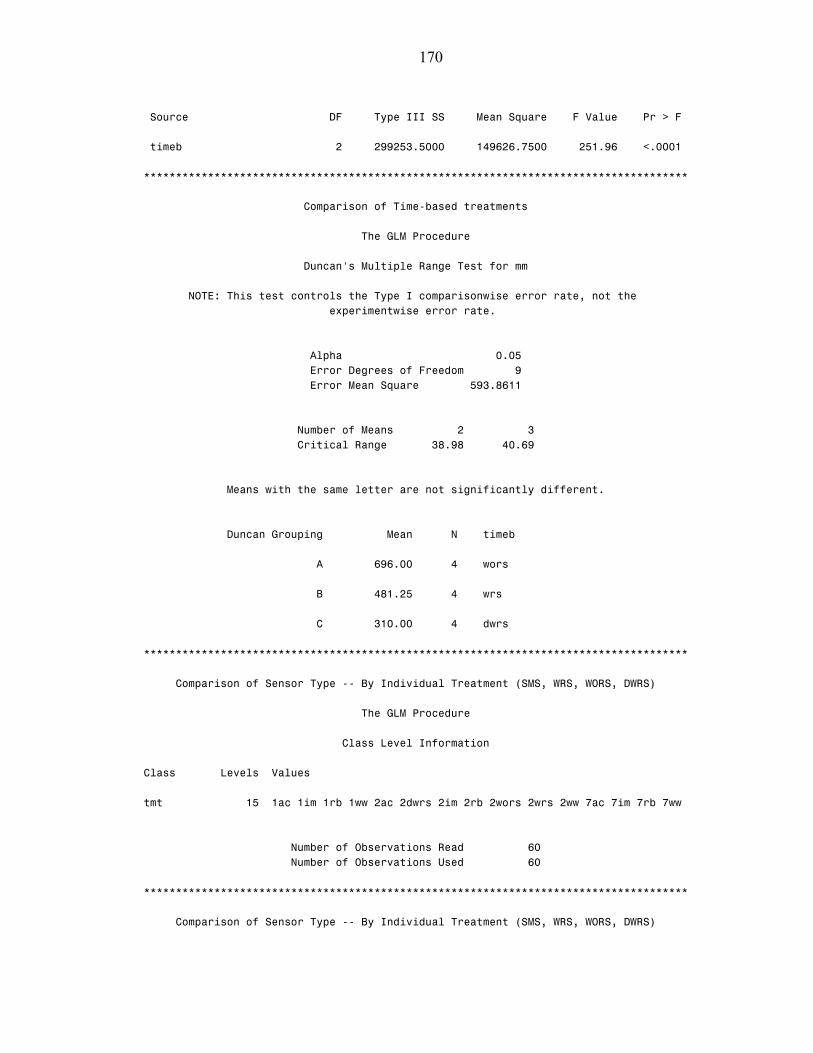
170
Source DF Type III SS Mean Square F Value Pr > F timeb 2 299253.5000 149626.7500 251.96 <.0001 ************************************************************************************* Comparison of Time-based treatments The GLM Procedure Duncan's Multiple Range Test for mm NOTE: This test controls the Type I comparisonwise error rate, not the experimentwise error rate. Alpha 0.05 Error Degrees of Freedom 9 Error Mean Square 593.8611 Number of Means 2 3 Critical Range 38.98 40.69 Means with the same letter are not significantly different. Duncan Grouping Mean N timeb A 696.00 4 wors B 481.25 4 wrs C 310.00 4 dwrs ************************************************************************************* Comparison of Sensor Type -- By Individual Treatment (SMS, WRS, WORS, DWRS) The GLM Procedure Class Level Information Class Levels Values tmt 15 1ac 1im 1rb 1ww 2ac 2dwrs 2im 2rb 2wors 2wrs 2ww 7ac 7im 7rb 7ww Number of Observations Read 60 Number of Observations Used 60 ************************************************************************************* Comparison of Sensor Type -- By Individual Treatment (SMS, WRS, WORS, DWRS)
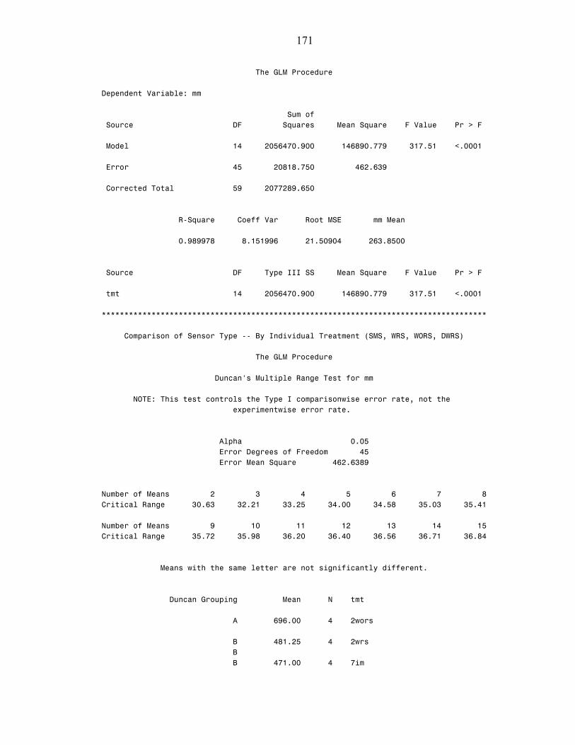
171
The GLM Procedure Dependent Variable: mm Sum of Source DF Squares Mean Square F Value Pr > F Model 14 2056470.900 146890.779 317.51 <.0001 Error 45 20818.750 462.639 Corrected Total 59 2077289.650 R-Square Coeff Var Root MSE mm Mean 0.989978 8.151996 21.50904 263.8500 Source DF Type III SS Mean Square F Value Pr > F tmt 14 2056470.900 146890.779 317.51 <.0001 ************************************************************************************* Comparison of Sensor Type -- By Individual Treatment (SMS, WRS, WORS, DWRS) The GLM Procedure Duncan's Multiple Range Test for mm NOTE: This test controls the Type I comparisonwise error rate, not the experimentwise error rate. Alpha 0.05 Error Degrees of Freedom 45 Error Mean Square 462.6389 Number of Means 2 3 4 5 6 7 8 Critical Range 30.63 32.21 33.25 34.00 34.58 35.03 35.41 Number of Means 9 10 11 12 13 14 15 Critical Range 35.72 35.98 36.20 36.40 36.56 36.71 36.84 Means with the same letter are not significantly different. Duncan Grouping Mean N tmt A 696.00 4 2wors B 481.25 4 2wrs B B 471.00 4 7im

172
B B 470.00 4 2im C 318.00 4 1im C C 310.00 4 2dwrs D 260.75 4 7ww E 209.25 4 1ww E E 196.00 4 2ac F 127.75 4 1rb G 95.25 4 1ac G G 93.75 4 2ww G H G 86.75 4 2rb H G H G 85.25 4 7rb H H 56.75 4 7ac

173
CUMULATIVE IRRIGATION DEPTH, YEAR 2005
options nodate nonumber center formdlim="*"linesize=85; data sms; input tmt$ day$ brand$ type$ based$ timeb$ mm; cards; /* Data is inputted here */ ; data sms2; set sms(where=(type = 'sms')); proc glm data=sms2; title 'Cumulative mm (March 25 - Aug 31/2005)'; class brand day; model mm = day brand day(brand) /ss3; test h=brand e=day(brand); means day/duncan; means brand/duncan; means brand/duncan e=day(brand); run; proc glm data=sms2; title 'Comparison of Interaction'; class brand day; model mm = brand*day /ss3; means brand*day/duncan; run; data sms3; set sms(where=(day = '1')); proc glm data=sms3; title 'Cumulative mm-- Once per Week'; class brand ; model mm = brand/ss3; means brand/duncan; run; data sms3; set sms(where=(day = '2')); proc glm data=sms3; title 'Cumulative mm-- Twice per Week'; class brand ; model mm = brand/ss3; means brand/duncan; run; data sms3; set sms(where=(day = '7')); proc glm data=sms3; title 'Cumulative mm-- Everyday'; class brand ; model mm = brand/ss3; means brand/duncan; run; data sms; set sms; proc glm data=sms; title 'Comparison of Time-based treatments'; class timeb; model mm = timeb /ss3; means timeb/duncan;

174
run; proc glm data=sms; title 'Comparison of Sensor Type -- By Individual Treatment (SMS, WRS, WORS, DWRS)'; class tmt; model mm = tmt /ss3; means tmt/duncan; run; ************************************************************************************* Cumulative mm (March 25 - Aug 31/2005) The GLM Procedure Class Level Information Class Levels Values brand 4 ac im rb ww day 3 1 2 7 Number of Observations Read 48 Number of Observations Used 48 ************************************************************************************* Cumulative mm (March 25 - Aug 31/2005) The GLM Procedure Dependent Variable: mm Sum of Source DF Squares Mean Square F Value Pr > F Model 11 1296396.167 117854.197 620.33 <.0001 Error 36 6839.500 189.986 Corrected Total 47 1303235.667 R-Square Coeff Var Root MSE mm Mean 0.994752 6.443418 13.78354 213.9167

175
Source DF Type III SS Mean Square F Value Pr > F day 2 128785.0417 64392.5208 338.93 <.0001 brand 3 923152.6667 307717.5556 1619.68 <.0001 day(brand) 6 244458.4583 40743.0764 214.45 <.0001 Tests of Hypotheses Using the Type III MS for day(brand) as an Error Term Source DF Type III SS Mean Square F Value Pr > F brand 3 923152.6667 307717.5556 7.55 0.0184 ************************************************************************************* Cumulative mm (March 25 - Aug 31/2005) The GLM Procedure Duncan's Multiple Range Test for mm NOTE: This test controls the Type I comparisonwise error rate, not the experimentwise error rate. Alpha 0.05 Error Degrees of Freedom 36 Error Mean Square 189.9861 Number of Means 2 3 Critical Range 9.88 10.39 Means with the same letter are not significantly different. Duncan Grouping Mean N day A 266.125 16 2 B 232.313 16 1 C 143.313 16 7 ************************************************************************************* Cumulative mm (March 25 - Aug 31/2005) The GLM Procedure Duncan's Multiple Range Test for mm NOTE: This test controls the Type I comparisonwise error rate, not the experimentwise error rate.
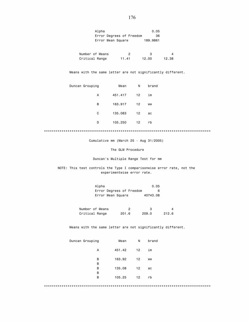
176
Alpha 0.05 Error Degrees of Freedom 36 Error Mean Square 189.9861 Number of Means 2 3 4 Critical Range 11.41 12.00 12.38 Means with the same letter are not significantly different. Duncan Grouping Mean N brand A 451.417 12 im B 163.917 12 ww C 135.083 12 ac D 105.250 12 rb ************************************************************************************* Cumulative mm (March 25 - Aug 31/2005) The GLM Procedure Duncan's Multiple Range Test for mm NOTE: This test controls the Type I comparisonwise error rate, not the experimentwise error rate. Alpha 0.05 Error Degrees of Freedom 6 Error Mean Square 40743.08 Number of Means 2 3 4 Critical Range 201.6 209.0 212.6 Means with the same letter are not significantly different. Duncan Grouping Mean N brand A 451.42 12 im B 163.92 12 ww B B 135.08 12 ac B B 105.25 12 rb *************************************************************************************
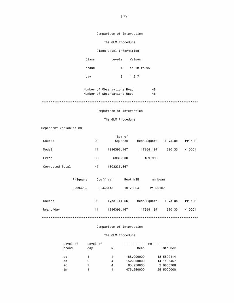
177
Comparison of Interaction The GLM Procedure Class Level Information Class Levels Values brand 4 ac im rb ww day 3 1 2 7 Number of Observations Read 48 Number of Observations Used 48 ************************************************************************************* Comparison of Interaction The GLM Procedure Dependent Variable: mm Sum of Source DF Squares Mean Square F Value Pr > F Model 11 1296396.167 117854.197 620.33 <.0001 Error 36 6839.500 189.986 Corrected Total 47 1303235.667 R-Square Coeff Var Root MSE mm Mean 0.994752 6.443418 13.78354 213.9167 Source DF Type III SS Mean Square F Value Pr > F brand*day 11 1296396.167 117854.197 620.33 <.0001 ************************************************************************************* Comparison of Interaction The GLM Procedure Level of Level of --------------mm------------- brand day N Mean Std Dev ac 1 4 188.000000 13.5892114 ac 2 4 152.000000 14.1185457 ac 7 4 65.250000 2.9860788 im 1 4 475.250000 25.5000000

178
im 2 4 634.750000 29.8817112 im 7 4 244.250000 5.0579970 rb 1 4 152.500000 10.5356538 rb 2 4 101.250000 1.2583057 rb 7 4 62.000000 3.5590261 ww 1 4 113.500000 9.3273791 ww 2 4 176.500000 7.1414284 ww 7 4 201.750000 7.4105780 ************************************************************************************* Cumulative mm-- Once per Week The GLM Procedure Class Level Information Class Levels Values brand 4 ac im rb ww Number of Observations Read 16 Number of Observations Used 16 ************************************************************************************* Cumulative mm-- Once per Week The GLM Procedure Dependent Variable: mm Sum of Source DF Squares Mean Square F Value Pr > F Model 3 325874.6875 108624.8958 420.65 <.0001 Error 12 3098.7500 258.2292 Corrected Total 15 328973.4375 R-Square Coeff Var Root MSE mm Mean 0.990581 6.917196 16.06951 232.3125 Source DF Type III SS Mean Square F Value Pr > F brand 3 325874.6875 108624.8958 420.65 <.0001

179
Cumulative mm-- Once per Week The GLM Procedure Duncan's Multiple Range Test for mm NOTE: This test controls the Type I comparisonwise error rate, not the experimentwise error rate. Alpha 0.05 Error Degrees of Freedom 12 Error Mean Square 258.2292 Number of Means 2 3 4 Critical Range 24.76 25.91 26.61 Means with the same letter are not significantly different. Duncan Grouping Mean N brand A 475.25 4 im B 188.00 4 ac C 152.50 4 rb D 113.50 4 ww ************************************************************************************* Cumulative mm-- Twice per Week The GLM Procedure Class Level Information Class Levels Values brand 4 ac im rb ww Number of Observations Read 16 Number of Observations Used 16
Cumulative mm-- Twice per Week The GLM Procedure Dependent Variable: mm Sum of
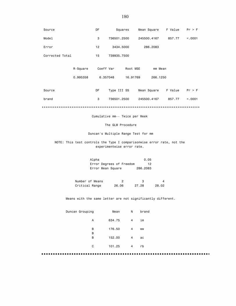
180
Source DF Squares Mean Square F Value Pr > F Model 3 736501.2500 245500.4167 857.77 <.0001 Error 12 3434.5000 286.2083 Corrected Total 15 739935.7500 R-Square Coeff Var Root MSE mm Mean 0.995358 6.357048 16.91769 266.1250 Source DF Type III SS Mean Square F Value Pr > F brand 3 736501.2500 245500.4167 857.77 <.0001 ************************************************************************************* Cumulative mm-- Twice per Week The GLM Procedure Duncan's Multiple Range Test for mm NOTE: This test controls the Type I comparisonwise error rate, not the experimentwise error rate. Alpha 0.05 Error Degrees of Freedom 12 Error Mean Square 286.2083 Number of Means 2 3 4 Critical Range 26.06 27.28 28.02 Means with the same letter are not significantly different. Duncan Grouping Mean N brand A 634.75 4 im B 176.50 4 ww B B 152.00 4 ac C 101.25 4 rb
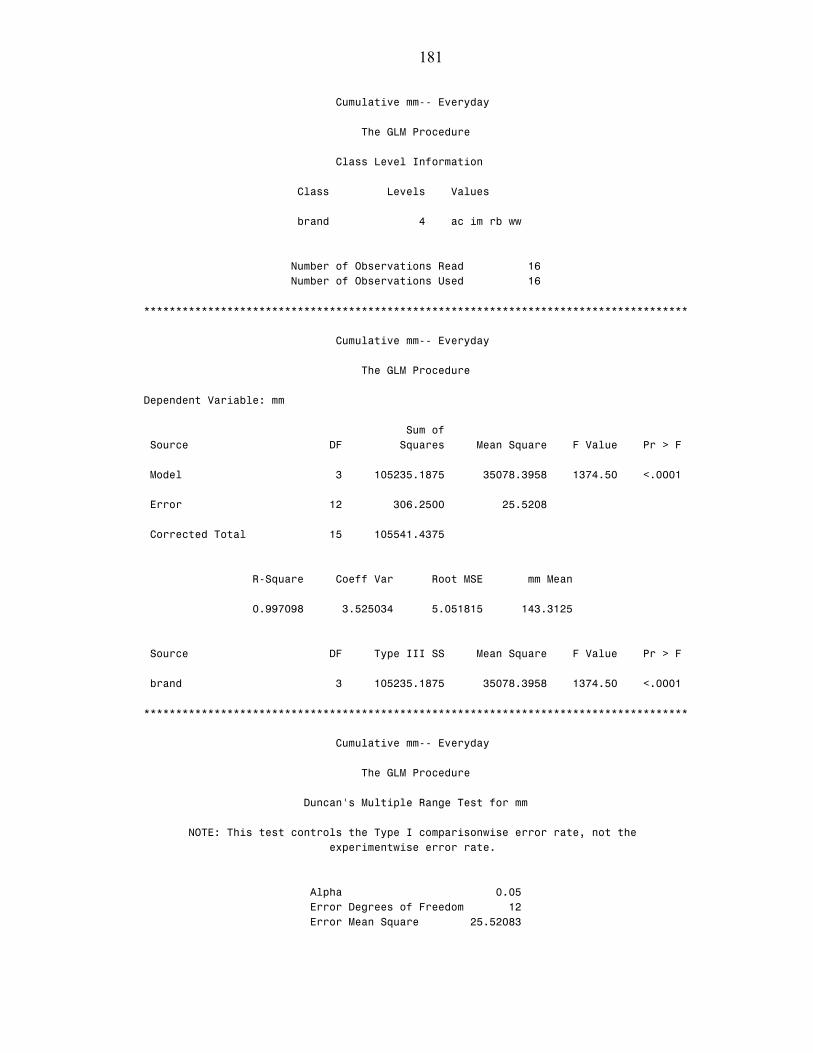
181
Cumulative mm-- Everyday The GLM Procedure Class Level Information Class Levels Values brand 4 ac im rb ww Number of Observations Read 16 Number of Observations Used 16 ************************************************************************************* Cumulative mm-- Everyday The GLM Procedure Dependent Variable: mm Sum of Source DF Squares Mean Square F Value Pr > F Model 3 105235.1875 35078.3958 1374.50 <.0001 Error 12 306.2500 25.5208 Corrected Total 15 105541.4375 R-Square Coeff Var Root MSE mm Mean 0.997098 3.525034 5.051815 143.3125 Source DF Type III SS Mean Square F Value Pr > F brand 3 105235.1875 35078.3958 1374.50 <.0001 ************************************************************************************* Cumulative mm-- Everyday The GLM Procedure Duncan's Multiple Range Test for mm NOTE: This test controls the Type I comparisonwise error rate, not the experimentwise error rate. Alpha 0.05 Error Degrees of Freedom 12 Error Mean Square 25.52083
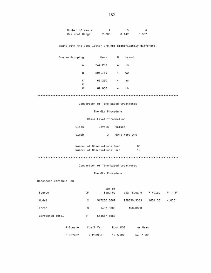
182
Number of Means 2 3 4 Critical Range 7.783 8.147 8.367 Means with the same letter are not significantly different. Duncan Grouping Mean N brand A 244.250 4 im B 201.750 4 ww C 65.250 4 ac C C 62.000 4 rb ************************************************************************************* Comparison of Time-based treatments The GLM Procedure Class Level Information Class Levels Values timeb 3 dwrs wors wrs Number of Observations Read 60 Number of Observations Used 12 ************************************************************************************* Comparison of Time-based treatments The GLM Procedure Dependent Variable: mm Sum of Source DF Squares Mean Square F Value Pr > F Model 2 517260.6667 258630.3333 1654.35 <.0001 Error 9 1407.0000 156.3333 Corrected Total 11 518667.6667 R-Square Coeff Var Root MSE mm Mean 0.997287 2.280936 12.50333 548.1667
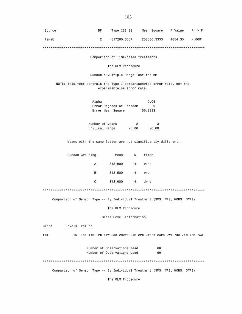
183
Source DF Type III SS Mean Square F Value Pr > F timeb 2 517260.6667 258630.3333 1654.35 <.0001 ************************************************************************************* Comparison of Time-based treatments The GLM Procedure Duncan's Multiple Range Test for mm NOTE: This test controls the Type I comparisonwise error rate, not the experimentwise error rate. Alpha 0.05 Error Degrees of Freedom 9 Error Mean Square 156.3333 Number of Means 2 3 Critical Range 20.00 20.88 Means with the same letter are not significantly different. Duncan Grouping Mean N timeb A 818.000 4 wors B 513.500 4 wrs C 313.000 4 dwrs ************************************************************************************* Comparison of Sensor Type -- By Individual Treatment (SMS, WRS, WORS, DWRS) The GLM Procedure Class Level Information Class Levels Values tmt 15 1ac 1im 1rb 1ww 2ac 2dwrs 2im 2rb 2wors 2wrs 2ww 7ac 7im 7rb 7ww Number of Observations Read 60 Number of Observations Used 60 ************************************************************************************* Comparison of Sensor Type -- By Individual Treatment (SMS, WRS, WORS, DWRS) The GLM Procedure
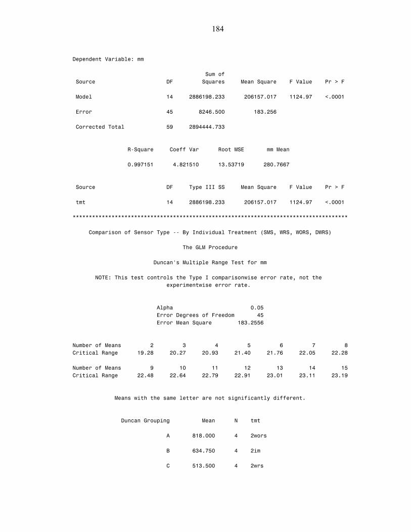
184
Dependent Variable: mm Sum of Source DF Squares Mean Square F Value Pr > F Model 14 2886198.233 206157.017 1124.97 <.0001 Error 45 8246.500 183.256 Corrected Total 59 2894444.733 R-Square Coeff Var Root MSE mm Mean 0.997151 4.821510 13.53719 280.7667 Source DF Type III SS Mean Square F Value Pr > F tmt 14 2886198.233 206157.017 1124.97 <.0001 ************************************************************************************* Comparison of Sensor Type -- By Individual Treatment (SMS, WRS, WORS, DWRS) The GLM Procedure Duncan's Multiple Range Test for mm NOTE: This test controls the Type I comparisonwise error rate, not the experimentwise error rate. Alpha 0.05 Error Degrees of Freedom 45 Error Mean Square 183.2556 Number of Means 2 3 4 5 6 7 8 Critical Range 19.28 20.27 20.93 21.40 21.76 22.05 22.28 Number of Means 9 10 11 12 13 14 15 Critical Range 22.48 22.64 22.79 22.91 23.01 23.11 23.19 Means with the same letter are not significantly different. Duncan Grouping Mean N tmt A 818.000 4 2wors B 634.750 4 2im C 513.500 4 2wrs

185
D 475.250 4 1im E 313.000 4 2dwrs F 244.250 4 7im G 201.750 4 7ww G H G 188.000 4 1ac H H 176.500 4 2ww I 152.500 4 1rb I I 152.000 4 2ac J 113.500 4 1ww J J 101.250 4 2rb K 65.250 4 7ac K K 62.000 4 7rb

186
CUMULATIVE IRRIGATION DEPTH, YEAR 2004 + 2005
options nodate nonumber center formdlim="*"linesize=85; data sms; input tmt$ day$ brand$ type$ based$ timeb$ mm; cards; /* Data is inputted here */ ; data sms2; set sms(where=(type = 'sms')); proc glm data=sms2; title 'TOTAL Cumulative mm (21 July 2004 - Aug 31/2005)'; class brand day; model mm = day brand day(brand) /ss3; test h=brand e=day(brand); means day/duncan; means brand/duncan; means brand/duncan e=day(brand); run; proc glm data=sms2; title 'Comparison of Interaction'; class brand day; model mm = brand*day /ss3; means brand*day/duncan; run; data sms3; set sms(where=(day = '1')); proc glm data=sms3; title 'Cumulative mm-- Once per Week'; class brand ; model mm = brand/ss3; means brand/duncan; run; data sms3; set sms(where=(day = '2')); proc glm data=sms3; title 'Cumulative mm-- Twice per Week'; class brand ; model mm = brand/ss3; means brand/duncan; run; data sms3; set sms(where=(day = '7')); proc glm data=sms3; title 'Cumulative mm-- Everyday'; class brand ; model mm = brand/ss3; means brand/duncan; run; data sms; set sms; proc glm data=sms; title 'Comparison of Time-based treatments'; class timeb;
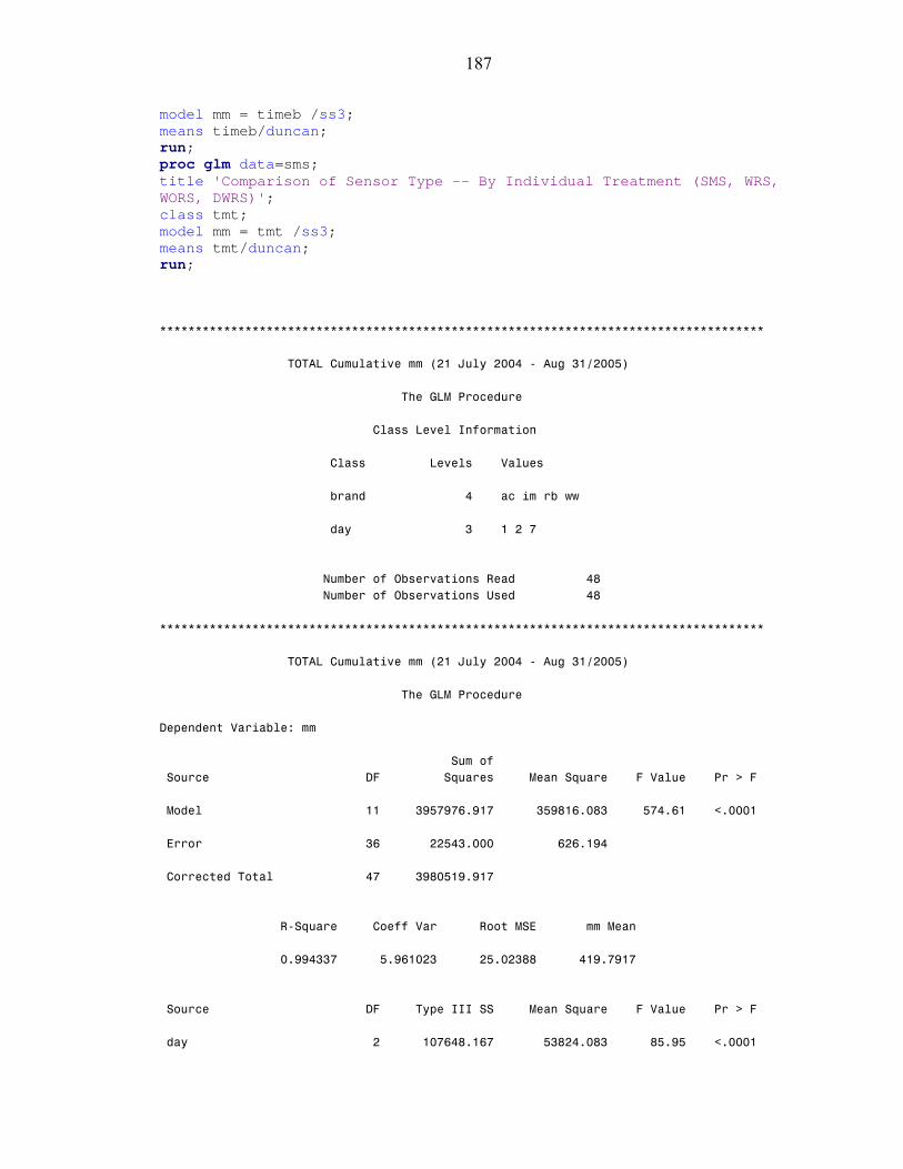
187
model mm = timeb /ss3; means timeb/duncan; run; proc glm data=sms; title 'Comparison of Sensor Type -- By Individual Treatment (SMS, WRS, WORS, DWRS)'; class tmt; model mm = tmt /ss3; means tmt/duncan; run; ************************************************************************************* TOTAL Cumulative mm (21 July 2004 - Aug 31/2005) The GLM Procedure Class Level Information Class Levels Values brand 4 ac im rb ww day 3 1 2 7 Number of Observations Read 48 Number of Observations Used 48 ************************************************************************************* TOTAL Cumulative mm (21 July 2004 - Aug 31/2005) The GLM Procedure Dependent Variable: mm Sum of Source DF Squares Mean Square F Value Pr > F Model 11 3957976.917 359816.083 574.61 <.0001 Error 36 22543.000 626.194 Corrected Total 47 3980519.917 R-Square Coeff Var Root MSE mm Mean 0.994337 5.961023 25.02388 419.7917 Source DF Type III SS Mean Square F Value Pr > F day 2 107648.167 53824.083 85.95 <.0001
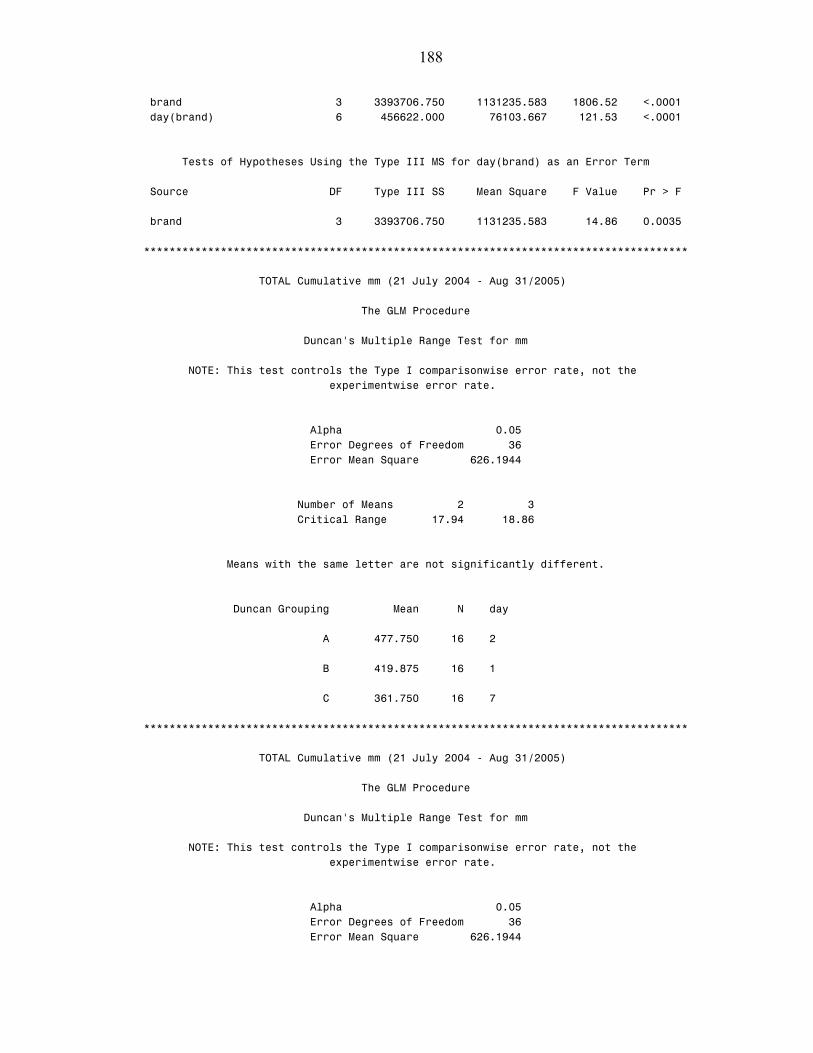
188
brand 3 3393706.750 1131235.583 1806.52 <.0001 day(brand) 6 456622.000 76103.667 121.53 <.0001 Tests of Hypotheses Using the Type III MS for day(brand) as an Error Term Source DF Type III SS Mean Square F Value Pr > F brand 3 3393706.750 1131235.583 14.86 0.0035 ************************************************************************************* TOTAL Cumulative mm (21 July 2004 - Aug 31/2005) The GLM Procedure Duncan's Multiple Range Test for mm NOTE: This test controls the Type I comparisonwise error rate, not the experimentwise error rate. Alpha 0.05 Error Degrees of Freedom 36 Error Mean Square 626.1944 Number of Means 2 3 Critical Range 17.94 18.86 Means with the same letter are not significantly different. Duncan Grouping Mean N day A 477.750 16 2 B 419.875 16 1 C 361.750 16 7 ************************************************************************************* TOTAL Cumulative mm (21 July 2004 - Aug 31/2005) The GLM Procedure Duncan's Multiple Range Test for mm NOTE: This test controls the Type I comparisonwise error rate, not the experimentwise error rate. Alpha 0.05 Error Degrees of Freedom 36 Error Mean Square 626.1944

189
Number of Means 2 3 4 Critical Range 20.72 21.78 22.47 Means with the same letter are not significantly different. Duncan Grouping Mean N brand A 871.08 12 im B 351.83 12 ww C 251.08 12 ac D 205.17 12 rb ************************************************************************************* TOTAL Cumulative mm (21 July 2004 - Aug 31/2005) The GLM Procedure Duncan's Multiple Range Test for mm NOTE: This test controls the Type I comparisonwise error rate, not the experimentwise error rate. Alpha 0.05 Error Degrees of Freedom 6 Error Mean Square 76103.67 Number of Means 2 3 4 Critical Range 275.6 285.6 290.6 Means with the same letter are not significantly different. Duncan Grouping Mean N brand A 871.1 12 im B 351.8 12 ww B B 251.1 12 ac B B 205.2 12 rb ************************************************************************************* Comparison of Interaction
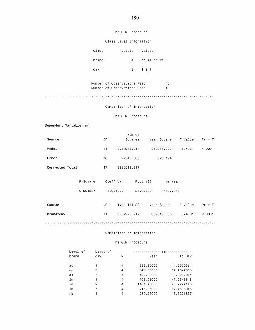
190
The GLM Procedure Class Level Information Class Levels Values brand 4 ac im rb ww day 3 1 2 7 Number of Observations Read 48 Number of Observations Used 48 ************************************************************************************* Comparison of Interaction The GLM Procedure Dependent Variable: mm Sum of Source DF Squares Mean Square F Value Pr > F Model 11 3957976.917 359816.083 574.61 <.0001 Error 36 22543.000 626.194 Corrected Total 47 3980519.917 R-Square Coeff Var Root MSE mm Mean 0.994337 5.961023 25.02388 419.7917 Source DF Type III SS Mean Square F Value Pr > F brand*day 11 3957976.917 359816.083 574.61 <.0001 ************************************************************************************* Comparison of Interaction The GLM Procedure Level of Level of --------------mm------------- brand day N Mean Std Dev ac 1 4 283.25000 14.6600364 ac 2 4 348.00000 17.4547033 ac 7 4 122.00000 3.8297084 im 1 4 793.25000 47.0345618 im 2 4 1104.75000 28.2297125 im 7 4 715.25000 57.4536045 rb 1 4 280.25000 16.5201897
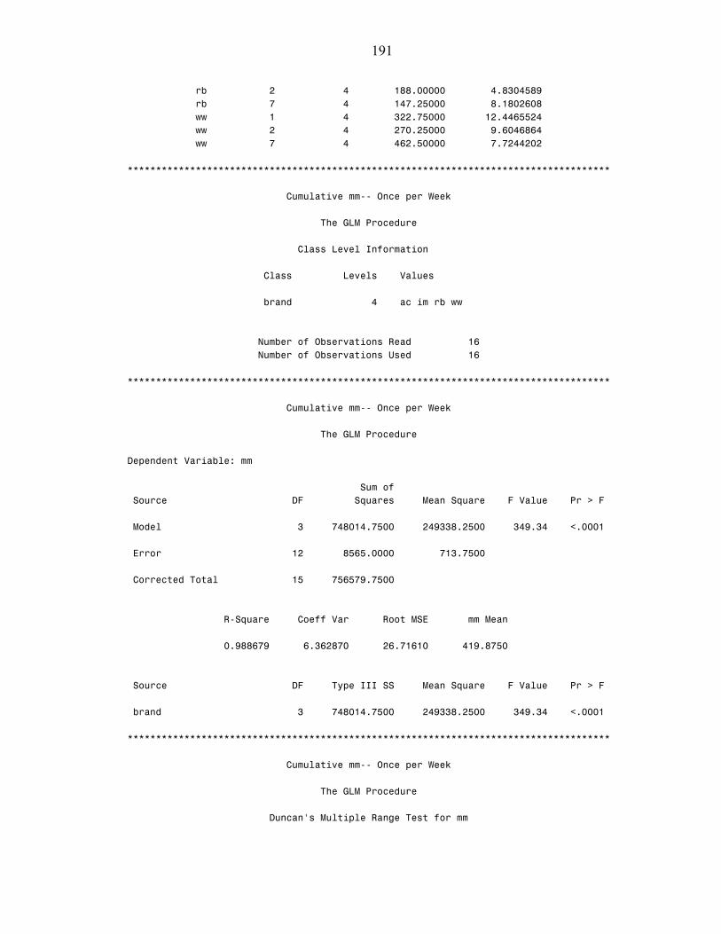
191
rb 2 4 188.00000 4.8304589 rb 7 4 147.25000 8.1802608 ww 1 4 322.75000 12.4465524 ww 2 4 270.25000 9.6046864 ww 7 4 462.50000 7.7244202 ************************************************************************************* Cumulative mm-- Once per Week The GLM Procedure Class Level Information Class Levels Values brand 4 ac im rb ww Number of Observations Read 16 Number of Observations Used 16 ************************************************************************************* Cumulative mm-- Once per Week The GLM Procedure Dependent Variable: mm Sum of Source DF Squares Mean Square F Value Pr > F Model 3 748014.7500 249338.2500 349.34 <.0001 Error 12 8565.0000 713.7500 Corrected Total 15 756579.7500 R-Square Coeff Var Root MSE mm Mean 0.988679 6.362870 26.71610 419.8750 Source DF Type III SS Mean Square F Value Pr > F brand 3 748014.7500 249338.2500 349.34 <.0001 ************************************************************************************* Cumulative mm-- Once per Week The GLM Procedure Duncan's Multiple Range Test for mm
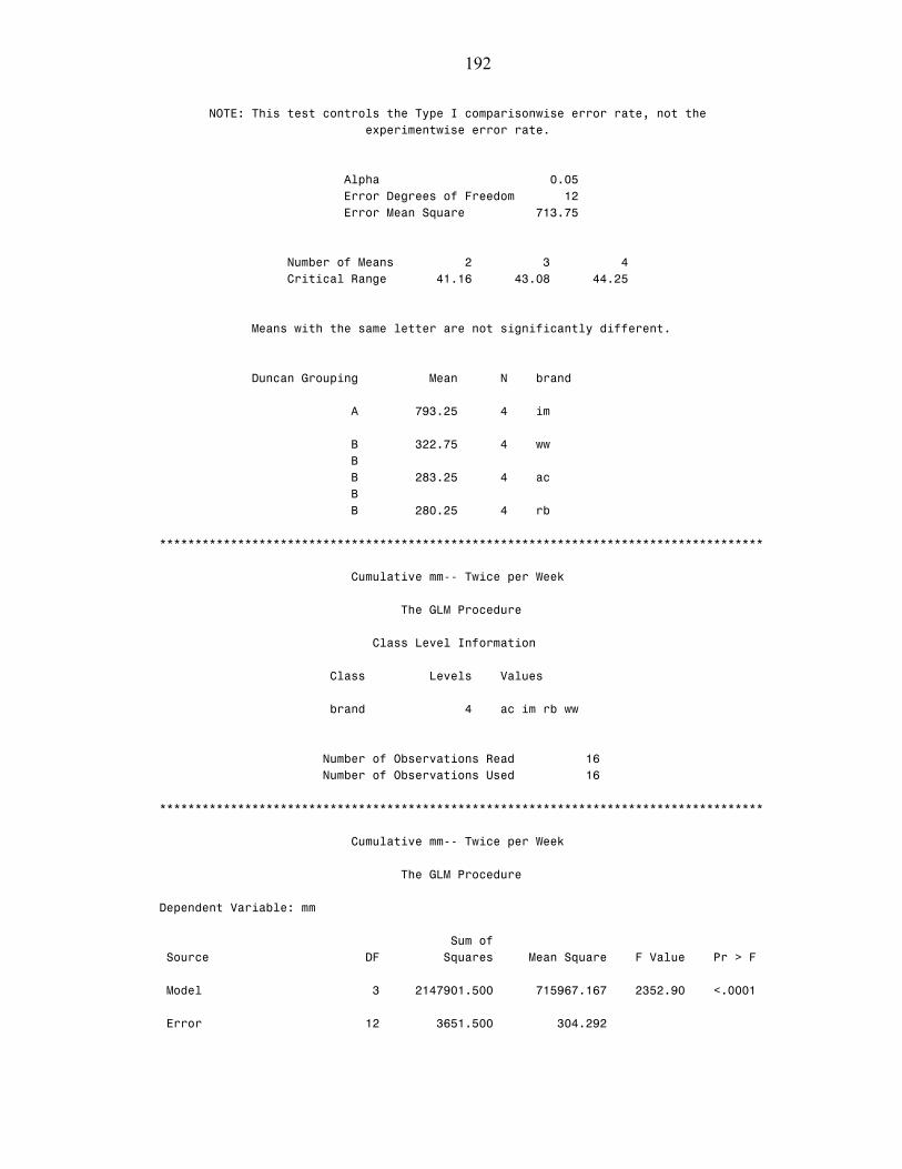
192
NOTE: This test controls the Type I comparisonwise error rate, not the experimentwise error rate. Alpha 0.05 Error Degrees of Freedom 12 Error Mean Square 713.75 Number of Means 2 3 4 Critical Range 41.16 43.08 44.25 Means with the same letter are not significantly different. Duncan Grouping Mean N brand A 793.25 4 im B 322.75 4 ww B B 283.25 4 ac B B 280.25 4 rb ************************************************************************************* Cumulative mm-- Twice per Week The GLM Procedure Class Level Information Class Levels Values brand 4 ac im rb ww Number of Observations Read 16 Number of Observations Used 16 ************************************************************************************* Cumulative mm-- Twice per Week The GLM Procedure Dependent Variable: mm Sum of Source DF Squares Mean Square F Value Pr > F Model 3 2147901.500 715967.167 2352.90 <.0001 Error 12 3651.500 304.292
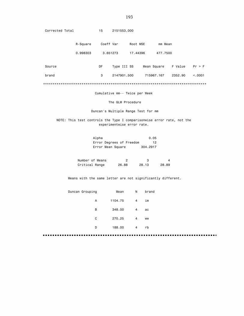
193
Corrected Total 15 2151553.000 R-Square Coeff Var Root MSE mm Mean 0.998303 3.651273 17.44396 477.7500 Source DF Type III SS Mean Square F Value Pr > F brand 3 2147901.500 715967.167 2352.90 <.0001 ************************************************************************************* Cumulative mm-- Twice per Week The GLM Procedure Duncan's Multiple Range Test for mm NOTE: This test controls the Type I comparisonwise error rate, not the experimentwise error rate. Alpha 0.05 Error Degrees of Freedom 12 Error Mean Square 304.2917 Number of Means 2 3 4 Critical Range 26.88 28.13 28.89 Means with the same letter are not significantly different. Duncan Grouping Mean N brand A 1104.75 4 im B 348.00 4 ac C 270.25 4 ww D 188.00 4 rb

194
Cumulative mm-- Everyday The GLM Procedure Class Level Information Class Levels Values brand 4 ac im rb ww Number of Observations Read 16 Number of Observations Used 16 ************************************************************************************* Cumulative mm-- Everyday The GLM Procedure Dependent Variable: mm Sum of Source DF Squares Mean Square F Value Pr > F Model 3 954412.5000 318137.5000 369.69 <.0001 Error 12 10326.5000 860.5417 Corrected Total 15 964739.0000 R-Square Coeff Var Root MSE mm Mean 0.989296 8.109189 29.33499 361.7500 Source DF Type III SS Mean Square F Value Pr > F brand 3 954412.5000 318137.5000 369.69 <.0001 ************************************************************************************* Cumulative mm-- Everyday The GLM Procedure Duncan's Multiple Range Test for mm NOTE: This test controls the Type I comparisonwise error rate, not the experimentwise error rate. Alpha 0.05 Error Degrees of Freedom 12 Error Mean Square 860.5417
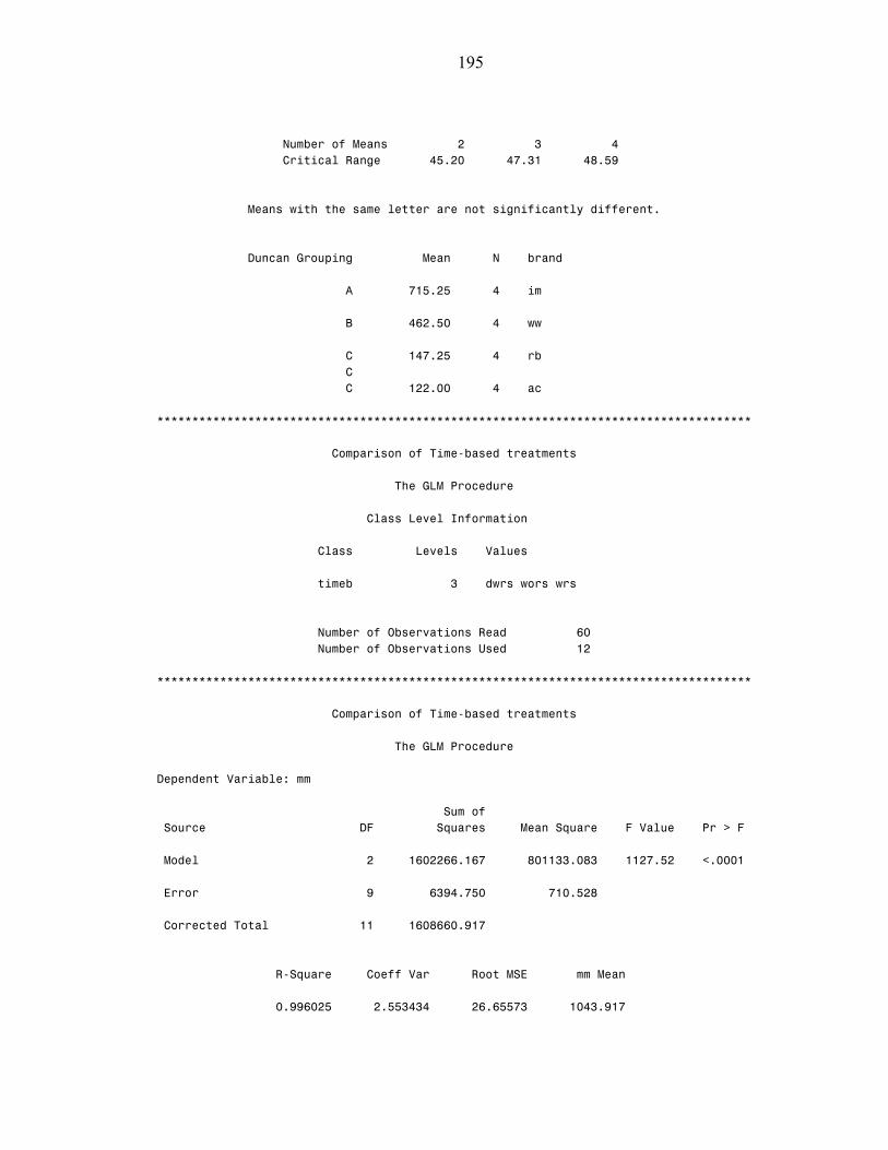
195
Number of Means 2 3 4 Critical Range 45.20 47.31 48.59 Means with the same letter are not significantly different. Duncan Grouping Mean N brand A 715.25 4 im B 462.50 4 ww C 147.25 4 rb C C 122.00 4 ac ************************************************************************************* Comparison of Time-based treatments The GLM Procedure Class Level Information Class Levels Values timeb 3 dwrs wors wrs Number of Observations Read 60 Number of Observations Used 12 ************************************************************************************* Comparison of Time-based treatments The GLM Procedure Dependent Variable: mm Sum of Source DF Squares Mean Square F Value Pr > F Model 2 1602266.167 801133.083 1127.52 <.0001 Error 9 6394.750 710.528 Corrected Total 11 1608660.917 R-Square Coeff Var Root MSE mm Mean 0.996025 2.553434 26.65573 1043.917

196
Source DF Type III SS Mean Square F Value Pr > F timeb 2 1602266.167 801133.083 1127.52 <.0001 ************************************************************************************* Comparison of Time-based treatments The GLM Procedure Duncan's Multiple Range Test for mm NOTE: This test controls the Type I comparisonwise error rate, not the experimentwise error rate. Alpha 0.05 Error Degrees of Freedom 9 Error Mean Square 710.5278 Number of Means 2 3 Critical Range 42.64 44.50 Means with the same letter are not significantly different. Duncan Grouping Mean N timeb A 1514.00 4 wors B 994.75 4 wrs C 623.00 4 dwrs ************************************************************************************* Comparison of Sensor Type -- By Individual Treatment (SMS, WRS, WORS, DWRS) The GLM Procedure Class Level Information Class Levels Values tmt 15 1ac 1im 1rb 1ww 2ac 2dwrs 2im 2rb 2wors 2wrs 2ww 7ac 7im 7rb 7ww Number of Observations Read 60 Number of Observations Used 60
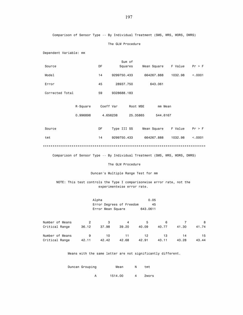
197
Comparison of Sensor Type -- By Individual Treatment (SMS, WRS, WORS, DWRS) The GLM Procedure Dependent Variable: mm Sum of Source DF Squares Mean Square F Value Pr > F Model 14 9299750.433 664267.888 1032.98 <.0001 Error 45 28937.750 643.061 Corrected Total 59 9328688.183 R-Square Coeff Var Root MSE mm Mean 0.996898 4.656238 25.35865 544.6167 Source DF Type III SS Mean Square F Value Pr > F tmt 14 9299750.433 664267.888 1032.98 <.0001 ************************************************************************************* Comparison of Sensor Type -- By Individual Treatment (SMS, WRS, WORS, DWRS) The GLM Procedure Duncan's Multiple Range Test for mm NOTE: This test controls the Type I comparisonwise error rate, not the experimentwise error rate. Alpha 0.05 Error Degrees of Freedom 45 Error Mean Square 643.0611 Number of Means 2 3 4 5 6 7 8 Critical Range 36.12 37.98 39.20 40.09 40.77 41.30 41.74 Number of Means 9 10 11 12 13 14 15 Critical Range 42.11 42.42 42.68 42.91 43.11 43.28 43.44 Means with the same letter are not significantly different. Duncan Grouping Mean N tmt A 1514.00 4 2wors
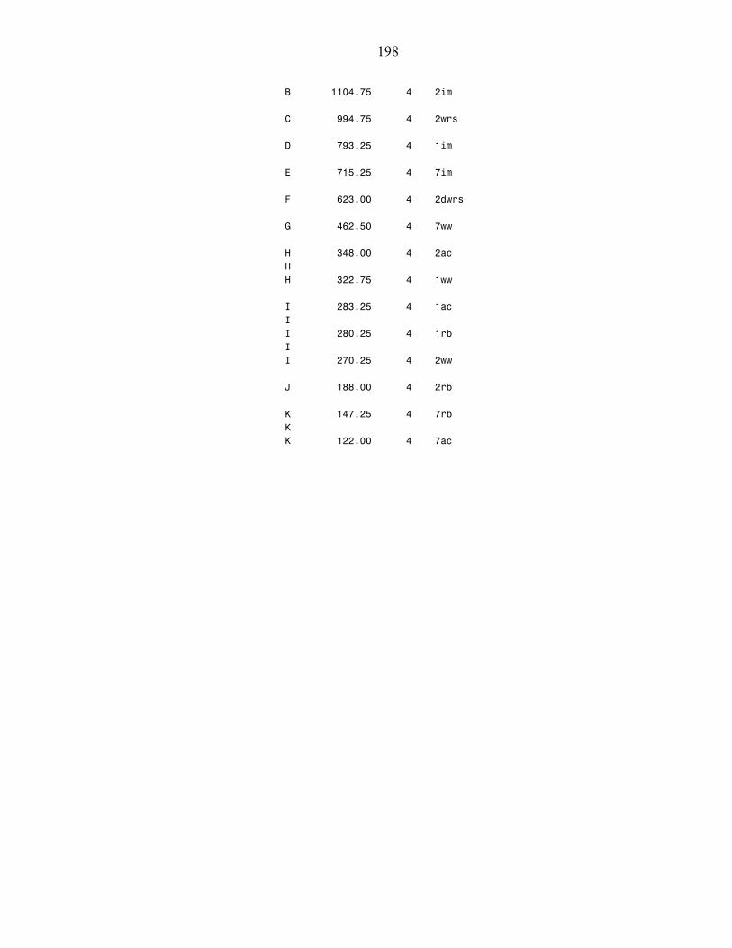
198
B 1104.75 4 2im C 994.75 4 2wrs D 793.25 4 1im E 715.25 4 7im F 623.00 4 2dwrs G 462.50 4 7ww H 348.00 4 2ac H H 322.75 4 1ww I 283.25 4 1ac I I 280.25 4 1rb I I 270.25 4 2ww J 188.00 4 2rb K 147.25 4 7rb K K 122.00 4 7ac

199
LIST OF REFERENCES
Allen R.G., L.S. Pereira, D. Raes and M. Smith. 1998. Crop evapotranspiration: Guidelines for computing crop requirements. Irrigation and Drainage Paper No. 56, FAO, Rome, Italy.
ASAE (American Society of Agricultural Engineers). 2000. Test procedure for determining the uniformity of water distribution of center pivot and lateral move irrigation machines equipped with spray or sprinkler nozzles. American Society of Agricultural Engineers Standards, ANSI/ASAE S436.1, 48th ed. St. Joseph, MI.
Augustin, B.J. 2000. Water requirements of Florida turfgrasses. BUL200, Institute of Food and Agricultural Sciences, University of Florida, Gainesville, FL. Available at: http://edis.ifas.ufl.edu/EP024. Accessed 7 January 2006.
Augustin, B.J. and G.H. Snyder. 1984. Moisture sensor-controlled irrigation for maintaining bermudagrass turf. Agron. J. 76: 848-850.
AWWA (American Water Works Association). 2004. Florida County restricts lawns. WaterWiser, September 2004. Available at: http://www.awwa.org/waterwiser/watch/archive.cfm. Accessed 7 January 2006
Baldwin, C.M., H. Liu, L.B. McCarty and W.L. Bauerle. 2005. Drought Tolerance of Six Bermudagrass Cultivars. TurfGrass Trends, Apr 1, 2005. Available at: http://www.turfgrasstrends.com/turfgrasstrends/article/articleDetail.jsp?id=156340. Accessed 7 January 2006.
Baum, M.C., M.D. Dukes, and G.L. Miller. 2003. Residential irrigation uniformity and efficiency in Florida. ASAE Meeting Paper FL03-100. St. Joseph, MI: ASAE.
Bausch, W.C., and T.M. Bernard. 1996. Validity of the Watermark sensor as a soil moisture measuring device. In: Proc. of the Intl. Conf. Evapotranspiration and Irrigation Scheduling. C.R. Camp, E.J. Sadler, and R.E. Yoder (eds.). St. Joseph, MI: ASAE. pp. 933-938.
Biran, I., B. Bravdo, I. Bushkin-Harav, and E. Rawitz. 1981. Water consumption and growth rate of 11 turfgrasses as affected by mowing height, irrigation frequency and soil moisture. Agron. J. 73: 85–90.

200
Boman, B., S. Smith, and B. Tullos. 2002. Control and automation in citrus microirrigation systems. CH194, Institute of Food and Agricultural Sciences, University of Florida, Gainesville, FL. Available at: http://edis.ifas.ufl.edu/CH194. Accessed 7 January 2006.
Bonos, S.A. and J.A. Murphy. 1999. Growth responses and performance of Kentucky bluegrass under summer stress. Crop Sci. 39:770-774.
Burney, L., T. Swihart, and J. Llewellyn. 1998. Water Supply Planning in Florida. Florida Water Resource Journal, October 1998: 27-28.
Burt, C.M.; A.J. Clemmens, and K.H. Strelkoff. 1997. Irrigation performance measurements: efficiency and uniformity. Journal of Irrigation and Drainage Engineering 123(6): 423-442.
Campbell, G.S., and D.J. Mulla. 1990. Measurement of soil water content and potential. In: Irrigation of agricultural crops. Agronomy Monograph No. 30. ASA-CSSA-SSSA, Madison, WI. pp. 127-142.
Carriker, R.R. 2000. Florida's water: supply, use, and public policy. Department of Food and Resource Economics, Report FE 207, University of Florida, Gainesville, FL.
Cassell, D.K., and A. Klute. 1986. Water potential: tensiometry. In: A. Klute (ed.) Methods of soil analysis. Part 1. 2nd ed. Agronomy 9. American Society of Agronomy, Madison, WI. pp. 563-596.
Charlesworth, P. 2000. Soil water monitoring. Irrigation Insights No.1. CSIRO Land and Water, Griffith, NSW. 96 p.
Christiansen, J.E. 1942. Irrigation by sprinkling. California Agric. Exp. Stn. Bull. 670. University of California, Berkley, CA.
Clark, G.A., C.D. Stanley, and D.N. Maynard. 1994. Tensiometer control vs. tomato crop coefficients for irrigation scheduling. ASAE Meeting Paper 94-2118, St. Joseph, MI: ASAE.
Colbaugh, P.F., and C.L. Elmore. 1985. Influence of water on pest activity. In V.A. Gibeault and S.T. Cockerham (ed.) Turfgrass water conservation. Cooperative Extension, University of California. pp. 113-129.
Davis, D.B., and P.H. Dernoeden, 1991. Summer patch and Kentucky bluegrass quality as influenced by cultural practices. Agron. J. 83:6702677.
Dewey, C. 2003. Sensors at work. Irrigation and green industry, September 2003. Available at: http://www.igin.com/Irrigation/0903sensors.html. Accessed 7 January 2006.
201
Dukes, M. D., E.H. Simonne, W.E. Davis, D.W. Studstill, and R. Hochmuth. 2003. Effect of sensor-based high frequency irrigation on bell pepper yield and water use. In Proceedings 2nd International Conference on Irrigation and Drainage, Phoenix, AZ: 665-674.
Dukes, M.D. and D. Z. Haman. 2002a. Operation of residential irrigation controllers. CIR1421, Institute of Food and Agricultural Sciences, University of Florida, Gainesville, FL.
Dukes, M.D. and D.Z. Haman. 2002b. Residential irrigation system rainfall shutoff devices. ABE325, Institute of Food and Agricultural Sciences, University of Florida, Gainesville, FL. Available at: http://edis.ifas.ufl.edu/AE221. Accessed 7 January 2006.
Dukes, M.D. and J.M. Scholberg. 2005. Soil moisture controlled subsurface drip irrigation on sandy soils. Applied Engineering in Agriculture 21(1): 89-101.
Dukes, M.D. and R. Muñoz-Carpena. 2005. Soil water sensor-based automatic irrigation of vegetable crops. In: Encyclopedia of Water Science. S.W. Trimble, B.A. Stewart and T.A. Howell (eds). Marcel-Dekker, Inc., NY. pp. 1-5.
Edis, R. and B. George, 2000. Time-domain reflectometry: an introduction. In: Soil water monitoring. P. Charlesworth (ed.). Irrigation Insights No.1. CSIRO Land and Water, Griffith, NSW. pp. 74-81.
Egbert, J.A., S. Baker, J.M. Baker. 1992. Calibration of Watermark soil moisture sensors for soil matrix potential and temperature. Plant Soil 143:213–217.
Eldredge, E.P., C.C. Schock, and T. Stieber. 1993. Calibration of granular matrix sensors for irrigation management. Agron. J. 85:1228–1232.
FDEP (Florida Department of Environmental Protection). 2002. Official notice of rule development: water shortage, NO 62-40.412. Publication Date: July 19, 2002. Available at: http://tlhora6.dep.state.fl.us/onw/publications/2-62-40RuleNoticewithruletextRevisedJuly2DT.pdf. Accessed 26 January 2005.
Figliola, R.S. and D.E. Beasley. 2000. Theory and design for mechanical measurements. 3rd ed. John Wiley and Sons, Inc. New York.
Florida Statutes, Part VI, Chapter 373.62. n.d. Water Conservation; automatic sprinkler systems. Available at: http://www.floridadep.org/water/stormwater/npdes/docs/ch373.pdf. Accessed 16 February 2006.
Florida Statutes. 2001. Changes to Chapter 373. Available at: http://www.dep.state.fl.us/cmp/federal/files/373ana01.pdf. Accessed 16 February 2006.

202
Gardner, W.H. 1986. Water content. In: Methods of soil analysis. Part 1. Physical and Mineralogical Methods, 2nd ed. A. Klute (ed.). Agronomy Monogr. No. 9. ASA and SSSA, Madison, WI. pp. 635–662.
Haley, M.B., M.D. Dukes, and G.L. Miller. 2006. Residential irrigation water use in Central Florida. Journal of Irrigation and Drainage Engineering (in press).
Hanson R.B., S. Orloff, and D. Peters. 2000a. Monitoring soil moisture helps refine irrigation management. Calif. Agric. 54:38–42
Hanson R.B., S. Orloff, and D. Peters. 2000b. Effectiveness of tensiometers and electrical resistance sensors varies with soil condition. Calif. Agric. 54:47–50
Harivandi, M.A., V.A. Gibeault, M.J. Henry, L. Wu, P.M. Geisel, and C.L. Unruh. 2001. Turfgrass selection for the home landscape. Publication 8035, University of California, Division of Agriculture and Natural Resources. Available at http://anrcatalog.ucdavis.edu/pdf/8035.pdf. Accessed 16 February 2006.
Hodges, A.W., J.J. Haydu, P.J. van Blokland, and A.P. Bell. 1994. Contribution of the turfgrass industry to Florida’s economy, 1991-1992: A value-added approach. University of Florida, Institute of Food and Agricultural Sciences, Food and Resource economics Department. Economic Report ER.
Hunter Industries, Inc. 2006. Products information. Available at: http://www.hunterindustries.com. Accessed 16 February 2006.
Irmak, S. and D.Z. Haman. 2001. Performance of the Watermark granular matrix sensor in sandy soils. Appl. Eng. Agric. 17: 787–795.
Irrigation Association. 2003. Landscape irrigation scheduling and water management. Irrigation Association Water Management Committee. Falls Church, VA.
Intrigliolo, D.S. and J.R. Castel. 2004. Continuous measurement of plant and soil water status for irrigation scheduling in plum. Irrig. Sci. 23: 93–102.
Jordan, J.E., R.H. White, D.M. Vietor, T.C. Hale, J.C. Thomas, and M.C. Engelke. 2003. Effect of irrigation frequency on turf quality, shoot density, and root length density of five bentgrass cultivars. Crop Science 43: 282–287. http://crop.scijournals.org/cgi/reprint/43/1/282
Kackley, K.E., A.P. Grybauskas, P.H. Dernoeden, and R.L. Hill. 1990. Role of drought stress in the development of summer patch in field inoculated Kentucky bluegrass. Phytopathology 80: 655-658.
Leib, B.G., M. Hattendorf, T. Elliott, and G. Matthews. 2002. Adoption and adaptation of scientific irrigation scheduling: trend from Washington, USA as of 1998. Agric. Water Manage. 55:105–120.

203
Leib, B.G., J.D. Jabro, and G.R. Matthews. 2003. Field evaluation and performance comparison of soil moisture sensors. Soil Science: 168(6) 396-408.
Ley, T.W., R.G. Stevens, R.R. Topielec and W.H. Neibling. 2000. Soil water monitoring and measurement. Pacific Northwest, WA. 33 p. Available at: http://cru.cahe.wsu.edu/CEPublications/pnw0475/pnw0475.html. Accessed 13 November 2003.
Marella, R.L. 1992. Water withdrawals, use, and trends in Florida, 1990. Water Resources Investigations Report 92-4140. United States Department of the Interior, U.S. Geological Survey, Tallahassee, FL.
Mayer, P.W., W.B. DeOreo, E.M. Opitz, J.C. Kiefer, W.Y. Davis, B. Dziegielewski, and J.O. Nelson. 1999. Residential end uses of water. American Water Works Association Research Foundation. Denver, CO.
McCann, I.R., D.C. Kincaid, and D. Wang. 1992. Operational characteristics of the watermark model 200 soil water potential sensor for irrigation management. Appl. Eng. Agric. 8:603–609
McCarty, L.B. 2005. Best Golf Course Management Practices. 2nd ed. Upper Saddle River, NJ. Prentice-Hall Inc.
Merriam, J.L., and J. Keller. 1978. Farm irrigation system evaluation: a guide for management. Department of Agricultural and Irrigation Engineering, Utah State University, Logan, UT.
Mitchell, A.R., and C.C. Shock. 1996. A Watermark datalogging system for ET measurement. In: Proc. of the Intl. Conf. Evapotranspiration and Irrigation Scheduling. C. R. Camp, E. J. Sadler, and R. E. Yoder (eds.). St. Joseph, MI: ASAE. pp. 468-473.
Muñoz-Carpena, R. 2004. Field devices for monitoring soil water content. BUL343, Institute of Food and Agricultural Sciences, University of Florida, Gainesville, FL. Available at: http://edis.ifas.ufl.edu/AE266. Accessed 7 January 2006.
Muñoz-Carpena, R. and M.D. Dukes. 2005. Automatic irrigation based on soil moisture for vegetable crops. ABE356, Institute of Food and Agricultural Sciences, University of Florida, Gainesville, FL. Available at: http://edis.ifas.ufl.edu/AE354. Accessed 7 January 2006.
Muñoz-Carpena, R., H. Bryan, W. Klassen, and M.D. Dukes. 2003. Automatic soil moisture-based drip irrigation for improving tomato production. Proceedings of the Florida State Horticultural Society 116: 80-85.
Muñoz-Carpena, R., M.D. Dukes, Y. Li, and W. Klassen. 2005. Field comparison of tensiometer and granular matrix sensor automatic drip irrigation on tomato. HortTechnology 15(3): 584-590.

204
National Research Council. 1996. A new era in irrigation. National Academies Press. Washington D.C.
NOAA (National Oceanic and Atmospheric Administration). 2003. Monthly station normals of temperature, precipitation, and heating and cooling degree days 1971 – 2000; 08 Florida. Climatography of The United States No. 81. 28p. Available at: http://hurricane.ncdc.noaa.gov/climatenormals/clim81/FLnorm.pdf. Accessed 29 April 2006.
Nogueira, L.C., M.D. Dukes, D.Z. Haman, J.M. Scholberg, and C. Cornejo. 2002. Data acquisition and irrigation controller based on CR10X datalogger and TDR sensor. Proceedings Soil and Crop Science Society of Florida 2002, 62: 38-46.
ODR (Office of Economic and Demographic Research.). 2006. Demographic Estimating Conference; Florida Demographic Forecast. Available at: http://edr.state.fl.us/conferences/population/demographic.htm Accessed 29 April 2006
Or, D. 2001. Who invented the tensiometer? Soil Sci. Soc. Am. J. 65: 1–3.
Pathan, S.M., L. Barton and T.D. Colmer. 2003. Evaluation of a soil moisture sensor to reduce water and nutrient leaching in turf. Horticulture Australia project number TU 02006. 21p.
Qualls, R.J., J.M. Scott, and W.B. DeOreo. 2001. Soil moisture sensors for urban landscape irrigation: effectiveness and reliability. Journal of the American Water Resources Association 37(3): 547-559.
Sarasota County. 2006. Water efficient landscaping ordinance; Ordinance #2001-081. Available at: http://sarasota.extension.ufl.edu/WEL/ord/docs/ord.htm. Accessed 24 April 2006.
SAS (Statistical Analysis System). 2000. SAS/STAT User’s Guide, Ver. 9. Cary, N.C.: SAS Institute, Inc.
Schmugge, T.J., T.J. Jackson, and H.L. McKim. 1980. Survey of methods for soil moisture determination. Water Resour. Res. 16: 961-979.
Seyfried, M.S. 1993. Field calibration and monitoring of soil water content with fiberglass electrical resistance sensors. Soil Sc. Soc. Am. J. 57: 1432–1436.
Shock, C.C., E. Fibert, and M. Saunders. 1996. Malheur Experiment Station Annual Report. Special Report 964, Oregon State University, Ontario, OR.
Shock, C.C., E.B.G. Feibert, and L.D. Saunders. 1998a. Onion yield and quality affected by soil water potential as irrigation threshold. HortScience 33: 1188–1191
205
Shock, C.C., E.B.G. Feibert, and L.D. Saunders. 1998b. Potato yield and quality response to deficit irrigation. HortScience 33: 655–659
Shock, C.C., E.B.G. Feibert, L.D. Saunders, and E.P. Eldredge. 2002. Automation of subsurface drip irrigation for crop research. In: Proceedings of the World Congress of Computers in Agriculture and Natural Resources. F.S. Zazueta and J. Xin eds. Iguacu Falls, Brazil. pp. 809-816
SJRWMD (Saint John’s River Water Management District). 2006. Waterwise Florida landscapes. Available at: http://sjrwmd.com/programs/outreach/conservation/landscape/principle5.html. Accessed 29 January 2006.
Skogley, C.R., and C.D. Sawyer. 1992. Field research. In: Turfgrass. Agron. Monogr. 32. D.V. Waddington, R.N. Carrow, and R.C. Shearman (eds.). ASA, CSSA, and SSSA, Madison, WI. pp. 589–614
Smajstrla, A.G. and R.C. Koo. 1986. Use of tensiometers for scheduling of citrus irrigation. Proceedings of the Florida State Horticultural Society 99: 51-56.
Smajstrla, A.G. and S.J. Locascio. 1994. Irrigation cutback effects on drip-irrigated tomato yields. Proceedings of the Florida State Horticultural Society 107: 113-118.
Solley, W.B., R.R. Pierce, and H.A. Perlman. 1998. Estimated use of water in the United States in 1995. United States Geological Survey Circular 1200. 78 p.
SWUCA (Southern Water Use Caution Area Recovery Strategy). 2006. Southwest Florida Water Management District. Revised Draft, March 2006. 145 p. Available at: http://www.swfwmd.state.fl.us/waterman/swuca/SWUCA.htm. Accessed 29 January 2006.
Taber H.G., V. Lawson, B. Smith, and D. Shogren. 2002. Scheduling microirrigation with tensiometers or Watermarks. Int. Water Irrig. 22: 22–26
Tampa Bay Water. 2005. Evaluating implementation of multiple irrigation and landscape ordinances in the Tampa Bay region. April 2005. Available at: http://www.tampabaywater.org/conservation/reportsdocs.aspx. Accessed 19 January 2006.
Thomas, B.D., E. Cummings, and W.H. Whittstruck. 1985. Soil survey of Alachua County, Florida. USDA/NRCS in cooperation with the University of Florida, Institute of Food and Agricultural Sciences, Soil Science Department and the Florida Department of Agriculture and Consumer Services.
Thomson, S.J., and C.F. Armstrong. 1987. Calibration of the Watermark model 200 soil moisture sensor. Applied Engineering in Agriculture 3(2): 186–189.
206
Thomson, S.J., T. Younos, and K. Wood. 1996. Evaluation of calibration equations and application methods for the Watermark granular matrix soil moisture sensor. Applied Engineering in Agriculture 12(1): 99–103.
Topp, G.C. 2003. State of the art of measuring soil water content. Hydrological Processes 17: 2993–2996.
Turgeon, A.J. 2005. Turfgrass Management. 7th ed. Upper Saddle River, NJ. Prentice- Hall Inc. 415p.
USCB (United States Census Bureau). 2004a. Population estimates. Washington, DC. Available at: http://www.census.gov/popest/estimates.php. Accessed 19 January 2006.
USCB (United States Census Bureau). 2004b. Housing unit estimates. Washington, DC. Available at: http://www.census.gov/popest/housing/. Accessed 19 January 2006.
USDA (United States Department of Agriculture). 1981. Land resource regions and major land resource areas of the united states. Soil Conservation Service Handbook 256. USDA, Washington, DC.
USDA (United States Department of Agriculture). 2003. Official soil series descriptions. Natural Resource and Conservation Service, Washington, DC. Available at: http://soils.usda.gov/technical/classification/osd/index.html. Accessed 13 April 2005.
USDA (United States Department of Agriculture). 2005. Florida State agriculture overview – 2005. National Agricultural Statistics Service. Available at: http://www.nass.usda.gov/Statistics_by_State/Ag_Overview/AgOverview_FL.pdf Accessed 13 April 2006.
Walker, J.P., G.R. Willgoose and J.D. Kalma. 2004. In situ measurement of soil moisture: a comparison of techniques. Journal of Hydrology 293: 85-99.
Whitcomb, J.B. 2005. Florida water rates evaluation of single-family homes. Southwest Florida Water Management District. Available at: http://www.swfwmd.state.fl.us/documents/reports/water_rate_report.pdf. Accessed 29 January 2006.
Yoder, R.E., D.L. Johnson, J.B. Wilkerson, and D.C. Yoder. 1998. Soil water sensor performance. Appl. Eng. Agric. 14: 121-133.
Youngner, V.B., A.W. Marsh, R.A. Strohman, V.A. Gibeault, and S. Spaulding. 1981. Water use and turfgrasses. Calif. Turfgrass Cult. 31: 1-4.

207
Zazueta, F.S., A.G. Smajstrla and G.A. Clark. 2002. Irrigation system controllers. SS-AGE-22, Institute of Food and Agricultural Sciences, University of Florida, Gainesville, FL. Available at: http://edis.ifas.ufl.edu/AE077. Accessed 10 April 2005.

208
BIOGRAPHICAL SKETCH
Bernard Cardenas-Lailhacar was born in Santiago, Chile. He received a Bachelor of
Science degree in agricultural engineering from the Universidad Austral de Chile. Later,
he accepted a graduate assistantship position in the Agricultural and Biological
Engineering Department at the University of Florida, and began studying toward a
Master of Science degree. On August 2006, Cardenas-Lailhacar received his M.Sc.
degree after defending his dissertation untitled “Sensor-based Automation of Irrigation of
Bermudagrass.”
While at the University of Florida, he obtained the highest grade of his class (GPA:
4.0), received five awards, and was invited to be part of two Honor Societies, on the basis
of his class performance. Moreover, he obtained the second place at the 2006 Graduate
Student Research Award of the American Society of Agricultural and Biological
Engineers (ASABE).
He is proficient in three languages (English, Spanish, and French), and has traveled
to 12 different countries in Europe and the Americas.