Embed Size (px)
Citation preview
DISCRETE APPLIED MATHEMATICS
Discrete Applied Mathematics 81 (1998) 133-139
Sensitivity analysis for knapsack problems: a negative result
Charles Blair*
Business Administration Department, University of Illinois, 1206 South Sixth St.- Box 8, Champaign, IL 61820, USA
Received 25 September 1996; received in revised form 4 April 1997; accepted 14 April 1997
Abstract
We show that, for any pair of knapsack problems, there is a single problem whose optimal solution corresponds to each problem of the pair, for two adjacent right-hand sides.
1. Introduction
We will be concerned with optimal solutions to (zero-one) knapsack problems:
max c cix, , iEI
c a-x. <b 2 IL > XiE{O,l}, iE1. (1) IEI
We will assume throughout that ai, ci, and b are natural numbers. Two knapsack
problems with identical a, c, and I but right-hand sides different by 1 will be called
“adjacent”. We are concerned with the relationship between optimal solutions to adja-
cent problems.
It is often the case that adjacent knapsack problems have the same optimal solution,
or that there is substantial overlap in the set of positive variables for the two problems.
However, it is easy to show that optimal solutions to adjacent problems may be com-
pletely unrelated. If, for some j E I, aj = b + 1 and cj is very large, then the optimal
solution to one problem has xj = 1, while the optimal solution to the other problem,
with xj = 0, is completely separate.
* E-mail: [email protected].
0166-218x198/$19.00 0 1998 Elsevier Science B.V. All rights reserved PII SOl66-218X(97)00080-2
134 C. Blair1 Discrete Applied Mathematics 81 (1998) 133-139
This example shows there may be no connection between adjacent knapsack prob-
lems, but is too simple to be interesting. The possibility remains that when optimal
solutions to adjacent problems are very different, one of the problems may be easy to
solve.
In this note, we show that there are adjacent knapsack problems with arbitrarily
complex solutions. For any pair of knapsack problems, new ai and ci are constructed
so that the optimal solutions to (1) for b + 1 and for b correspond to the optimal
solutions of the given pair of problems.
An integer programming problem with a single constraint arises from (1) if we
replace the requirement xi E (0, 1) by the requirement that xi is a non-negative in-
teger. A similar result can be established for such problems. We refer to [3] for
details.
2. The main result
We will refer to a knapsack problem (1) by the 4-tuple (a, c,Z, b). Two such problems
with right-hand sides L and M will be denoted by (a, c, II, L) and (a, c, Iz,M), where
Ii and I, are disjoint index sets.
We will be constructing adjacent knapsack problems from two arbitrary given prob-
lems. The adjacent problems will have variables corresponding to each of the given
problems, together with some additional variables. The new variables will correspond
to the index sets J1 and Jz in the statement of Theorem 1.
Theorem 1. Suppose we are given any two knapsack problems (a,c,Zl,L) and (a, c,Z2,A4). We can construct a knapsack problem (a’, c’, I, b), with I=Il U J1 U 12 U J2,
such that: 1. For some natural numbers T and U, a; = Tai for i E I,, and af = Uai for i E Ix. 2. If x is optimal for (a’, c’,I, b), then xi = 0 for all i E 12 U J2, and x is an optimal
solution to (a, c, II, L). 3. If x is optimal for (a’, cl, I, b + l), then xi = 0 for all i E I, U J1, and x is an optimal
solution to (a, c, I2,M). 4. (a’, cl, J1 U J2, b) is easy to solve for any b.
Moreover, (a’, c’,Z, b) may be easily constructed without knowing the optimal solu-
tions of the two original problems.
Condition 1 insures that the constraint coefficients of the original problems are pre-
served, up to multiplication by constants. Conditions 2 and 3 show that the optimal
solutions for right-hand sides b and b + 1 come from the original problems. Since
these were arbitrarily chosen, they may be completely unrelated and may both be com-
plicated. Condition 4 suggests that the difficulty of the newly constructed problems
comes from the variables of the two original problems, rather than from the variables
corresponding to J1 U J2.
C. Blair1 Discrete Applied Mathematics 81 (1998) 133-139 135
3. Some lemmas
It will be necessary to replace a problem (1) by an equivalent problem in which
b is replaced by a new right-hand side b’> b. This can be done by adding one new
variable.
Lemma 2. Let 0 6 I. We can find a0 and co such that x is an optimal solution to
max c CiXi ) iE{O}UI
C aixi <b’,xi E (0, I}, i E (0) “1 (2) iE{O}UI
if and only if x0 = 1 and (xi, i E I) is an optimal solution to (1). Moreover, a0 and
CO can be found without knowing the optimal solution to (1).
Proof, Let a0 = b’ - b and CO be sufficiently large so that any feasible solution to (2)
with x0 = 0 will be smaller than having x0 = 1, even if all other xi = 0. A simple choice
for CO would be 1 + CiEI ci. 0
We want to confine our attention to problems (1) in which the constraint is tight for
any optimal solution x*, i.e., C six* = b. For any problem, we can create an equivalent
new problem with log, b additional variables for which this is the case.
Lemma 3. For a knapsack problem (1) let 2j <b <2j+‘. Let J = (0,. . . , j} and as-
sume I n J = 8. Then (xi, i E I U J), is an optimal solution to:
max C (Ci + Ui)Xi + C 2’Xi (3) iEl iEJ
C aixi + C 2’xi<b (4) iEl iEJ
xiE{O,l}, iEZUJ (5)
if and only if(4) is tight (satis$ed as an equation) and (xi, i E Z) is an optimal solution
to (1).
Proof. Let (x1?, i E I) be an optimal solution to (1 ), with objective value v* = CiE1 cix*.
Let (xl?, i E J) be such that
C 2’~: = b - C aixr. iCJ iEI
If (Xi, i E I U J) is any feasible solution to (4) and (5), then
C (Ci + ai)& + C 2’Xi < C cixi + b iEI iEJ iEI
(6)
136 C. Blair I Discrete Applied Mathematics 81 (1998) 133-139
<v*+b (7)
= C (ci + Ui)X* + C 2’X*, (8) iEI iEJ
so x* is an optimal solution to (3)-(5).
Conversely, if x is feasible, but (4) is not tight or xi,, CiXi <v*, then (6) or (7)
will be a strict inequality, and x will not be optimal. 0
The use of powers of 2 is a common device in establishing NP-completeness results,
e.g. [6, Theorem 3.51.
We will need a simple result from number theory.
Lemma 4. Suppose that L, a, 1, b are non-negative integers, and that
(L+2)m+(L+ l)P=b.
If b = (L + 1)2 or b = L2 + 2L, then CI = 0 or j3 = 0, respectively.
(9)
Proof. If b=(L + 1)2, (9) implies
a=(L+l)(L+l-_-Lx),
i.e., M is divisible by L + 1. Since cx > L + 1 would imply p < 0, we must have CI = 0.
The case b = L2 + 2L is similar, based on showing /I is divisible by L + 2. q
Our next result shows how to achieve the main conclusions of Theorem 1 when we
start with a pair of problems that have some special properties.
Lemma 5. Suppose II n I2 = 0 and that the knapsack problems:
max c CiXi, max C CiXi,
iEIl iCI2
c UiXi <L, c UiXi <L + 1, (10)
iEIl iEI2
Xi E (0, I}, Xi E (0, I}
have the property that every optimal solution to each problem satisfies its constraint as an equality. Choose a natural number N so that
N> C ci. (11) iEIl VI2
LetL1=L,L2=L+1,b~=L2+2L,andb2=(L+1)2=bl+1. Thenxwillbean optimal solution to:
maxC(ci+N(L+2)ai)xi+C(ci+N(L+l)ai)Xi, (12) iEIl iEI2
C. Blair1 Discrete Applied Mathematics 81 (1998) 133-139 137
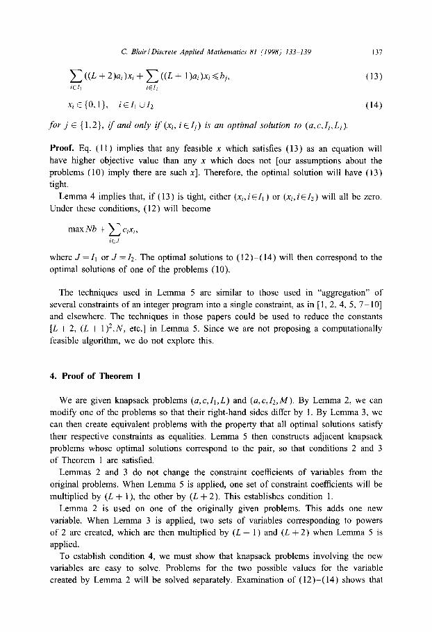
C((L+2)Qi)%+C((L+ l)Qi)xidbj, (13) iEIl iEI2
Xi E (0, l}, iEZr UI* (14)
for j E {1,2}, ifand only if(xi, ills) 1s an optimal solution to (a, C, Ij, Lj).
Proof. Eq. (11) implies that any feasible x which satisfies (13) as an equation will
have higher objective value than any x which does not [our assumptions about the
problems (10) imply there are such x]. Therefore, the optimal solution will have ( 13)
tight.
Lemma 4 implies that, if (13) is tight, either (x,,i~Il) or (xi, i~lz) will all be zero.
Under these conditions, (12) will become
max A% + C CjXi,
LEJ
where J =I1 or J =Z,. The optimal solutions to (12)-(14) will then correspond to the
optimal solutions of one of the problems (10).
The techniques used in Lemma 5 are similar to those used in “aggregation” of
several constraints of an integer program into a single constraint, as in [ 1, 2, 4, 5, 7- lo]
and elsewhere. The techniques in those papers could be used to reduce the constants
[L + 2, (L + 1)2,N, etc.] in Lemma 5. Since we are not proposing a computationally
feasible algorithm, we do not explore this.
4. Proof of Theorem 1
We are given knapsack problems (a,c,Il,L) and (LI,c,I~,M). By Lemma 2, we can
modify one of the problems so that their right-hand sides differ by 1. By Lemma 3, we
can then create equivalent problems with the property that all optimal solutions satisfy
their respective constraints as equalities. Lemma 5 then constructs adjacent knapsack
problems whose optimal solutions correspond to the pair, so that conditions 2 and 3
of Theorem 1 are satisfied.
Lemmas 2 and 3 do not change the constraint coefficients of variables from the
original problems. When Lemma 5 is applied, one set of constraint coefficients will be
multiplied by (L + l), the other by (L + 2). This establishes condition 1.
Lemma 2 is used on one of the originally given problems. This adds one new
variable. When Lemma 3 is applied, two sets of variables corresponding to powers
of 2 are created, which are then multiplied by (L + 1) and (L + 2) when Lemma 5 is
applied.
To establish condition 4, we must show that knapsack problems involving the new
variables are easy to solve. Problems for the two possible values for the variable
created by Lemma 2 will be solved separately. Examination of (12)-(14) shows that
138 C. BIairIDiscrete Applied Mathematics 81 (1998) 133-139
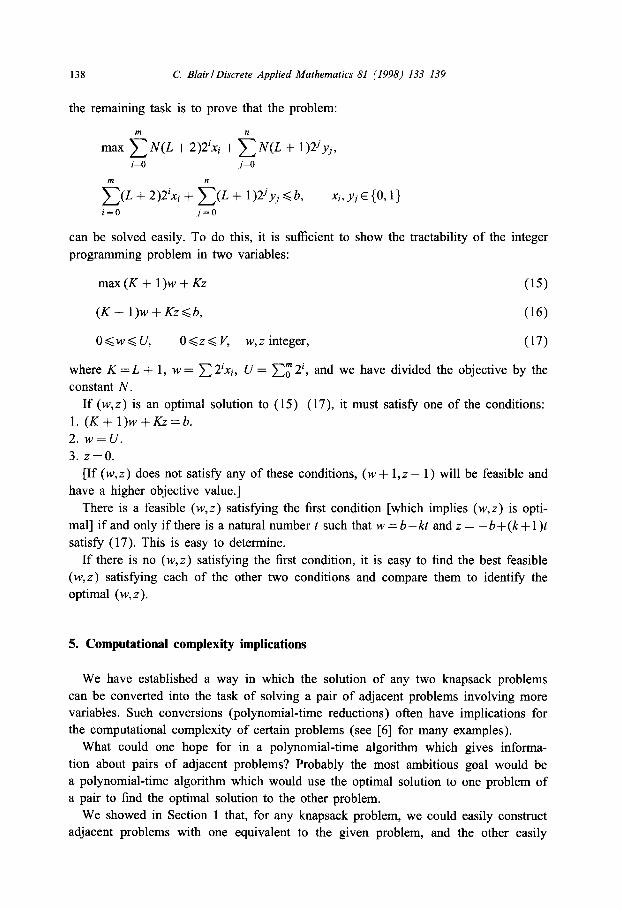
the remaining task is to prove that the problem:
max e N(L + 2)2’Xj + 2 N(L + 1)2j&, i=O j=O
e(L+2)2’Xi+k(L+ 1)2jyj<b, Xi,vjE{O,l} i=o j=O
can be solved easily. To do this, it is sufficient to show the tractability of the integer
programming problem in
max(K + 1)w +Kz
(K + 1)w +Kz<b,
two variables:
(15)
(16)
o<w<u, 0 <z < V, w,z integer, (17)
where K = L + 1, w = C 2iXi, U = Cl: 2’, and we have divided the objective by the
constant N.
If (w,z) is an optimal solution to (15)-(17), it must satisfy one of the conditions:
1. (K+ l)w+Kz=b.
2. w=u.
3. z=o.
[If (w,z) does not satisfy any of these conditions, (w + 1,z - 1) will be feasible and
have a higher objective value.]
There is a feasible (w,z) satisfying the first condition [which implies (w,z) is opti-
mal] if and only if there is a natural number t such that w = b-kt and z = -b+(k+ 1 )t
satisfy (17). This is easy to determine.
If there is no (w,z) satisfying the first condition, it is easy to find the best feasible
(w,z) satisfying each of the other two conditions and compare them to identify the
optimal (w, z).
5. Computational complexity implications
We have established a way in which the solution of any two knapsack problems
can be converted into the task of solving a pair of adjacent problems involving more
variables. Such conversions (polynomial-time reductions) often have implications for
the computational complexity of certain problems (see [6] for many examples).
What could one hope for in a polynomial-time algorithm which gives informa-
tion about pairs of adjacent problems? Probably the most ambitious goal would be
a polynomial-time algorithm which would use the optimal solution to one problem of
a pair to find the optimal solution to the other problem.
We showed in Section 1 that, for any knapsack problem, we could easily construct
adjacent problems with one equivalent to the given problem, and the other easily
C. Blair1 Discrete Applied Mathematics 81 (1998) 133-139 139
solvable. Thus, the suggested algorithm would be capable of solving any knapsack
problem. This is unlikely, given the NP-completeness of knapsack problems.
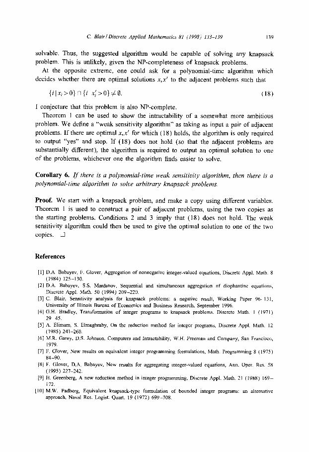
At the opposite extreme, one could ask for a polynomial-time algorithm which
decides whether there are optimal solutions x,x’ to the adjacent problems such that
I conjecture that this problem is also NP-complete.
Theorem 1 can be used to show the intractability of a somewhat more ambitious
problem. We define a “weak sensitivity algorithm” as taking as input a pair of adjacent
problems. If there are optimal x,x’ for which (18) holds, the algorithm is only required
to output “yes” and stop. If (18) does not hold (so that the adjacent problems are
substantially different), the algorithm is required to output an optimal solution to one
of the problems, whichever one the algorithm finds easier to solve.
Corollary 6. If there is a polynomial-time weak sensitivity algorithm, then there is u
polynomial-time algorithm to solve arbitrary knapsack problems.
Proof. We start with a knapsack problem, and make a copy using different variables.
Theorem 1 is used to construct a pair of adjacent problems, using the two copies as
the starting problems. Conditions 2 and 3 imply that (18) does not hold. The weak
sensitivity algorithm could then be used to give the optimal solution to one of the two
copies. 0
References
[l] D.A. Babayev, F. Glover, Aggregation of nomregative integer-valued equations, Discrete Appl. Math. 8 (1984) 125-130.
[2] D.A. Babayev, S.S. Mardanov, Sequential and simultaneous aggregation of diophantine equations, Discrete Appl. Math. 50 (1994) 209-220.
[3] C. Blair, Sensitivity analysis for knapsack problems: a negative result, Working Paper 96-131, University of Illinois Bureau of Economics and Business Research, September 1996.
[4] G.H. Bradley, Transformation of integer programs to knapsack problems, Discrete Math. I (1971) 29-45.
[5] A. Elimam, S. Elmaghraby, On the reduction method for integer programs, Discrete Appt. Math. 12 (1985) 241-260.
[6] M.R. Garey, D.S. Johnson, Computers and Intractability, W.H. Freeman and Company, San Francisco, 1979.
[7] F. Glover, New results on equivalent integer programming formulations, Math. Programming 8 (1975) 84-90.
[8] F. Glover, D.A. Babayev, New results for aggregating integer-valued equations, Ann. Oper. Res. 58 (1995) 227-242.
[9] H. Greenberg, A new reduction method in integer programming, Discrete Appl. Math. 21 ( 1988) 169- 172.
[IO] M.W. Padberg, Equivalent knapsack-type formulation of bounded integer programs: an alternative approach, Naval Res. Logist. Quart. 19 (1972) 699-708.