Embed Size (px)
DESCRIPTION
Sensitivity Analysis A. Saltelli European Commission, Joint Research Centre of Ispra, Italy [email protected] Toulouse, February 3, 2006. Outline Definitions and requirements Suggested practices. Why uncertainty and sensitivity analyses?. Why sensitivity analysis?. - PowerPoint PPT Presentation
Citation preview

http://www.jrc.cec.eu.int/uasa 1
Sensitivity Analysis
A. SaltelliEuropean Commission,
Joint Research Centre of Ispra, Italy
Toulouse, February 3, 2006

http://www.jrc.cec.eu.int/uasa 2
Outline •Definitions and requirements •Suggested practices

http://www.jrc.cec.eu.int/uasa 3
Why uncertainty and sensitivity analyses?
http://www.jrc.cec.eu.int/uasa 4
Would you go to an orthopaedist who did not use X-rays? (J.M. Furbinger)
Why sensitivity analysis?
http://www.jrc.cec.eu.int/uasa 5
Sometime scientific theories compete as to which best describe the evidence. This competition takes place in the space of uncertainties (otherwise there would be no competition).
Sensitivity analysis can help make the overall appreciation of the merits of each theory clearer, by mapping a theory’s assumptions onto its inferences.
This may even lead to the falsification of one of the theories.
Why sensitivity analysis?
http://www.jrc.cec.eu.int/uasa 6
Sometime scientific information feeds into the policy process. When this is the case, all parties manipulate uncertainty.
Uncertainty cannot be resolved into certitude in most instances. Instead, transparency can be offered by sensitivity analysis. Transparency is what is needed to ensure that the negotiating parties do retain science as an ingredient of decision making.
Why sensitivity analysis?
http://www.jrc.cec.eu.int/uasa 7
• A Definition
[Global*] sensitivity analysis: “The study of how the uncertainty in the output of a model (numerical or otherwise) can be apportioned to different sources of uncertainty in the model input”
*Global could be an unnecessary specification, were it not for the fact that most analysis met in the literature are local or one-factor-at-a-time … but not at this workshop!
http://www.jrc.cec.eu.int/uasa 8
One factor at a time methods are those whereby each input variable is varied or perturbed in turn and the effect on the output measured.
OAT methods
http://www.jrc.cec.eu.int/uasa 9
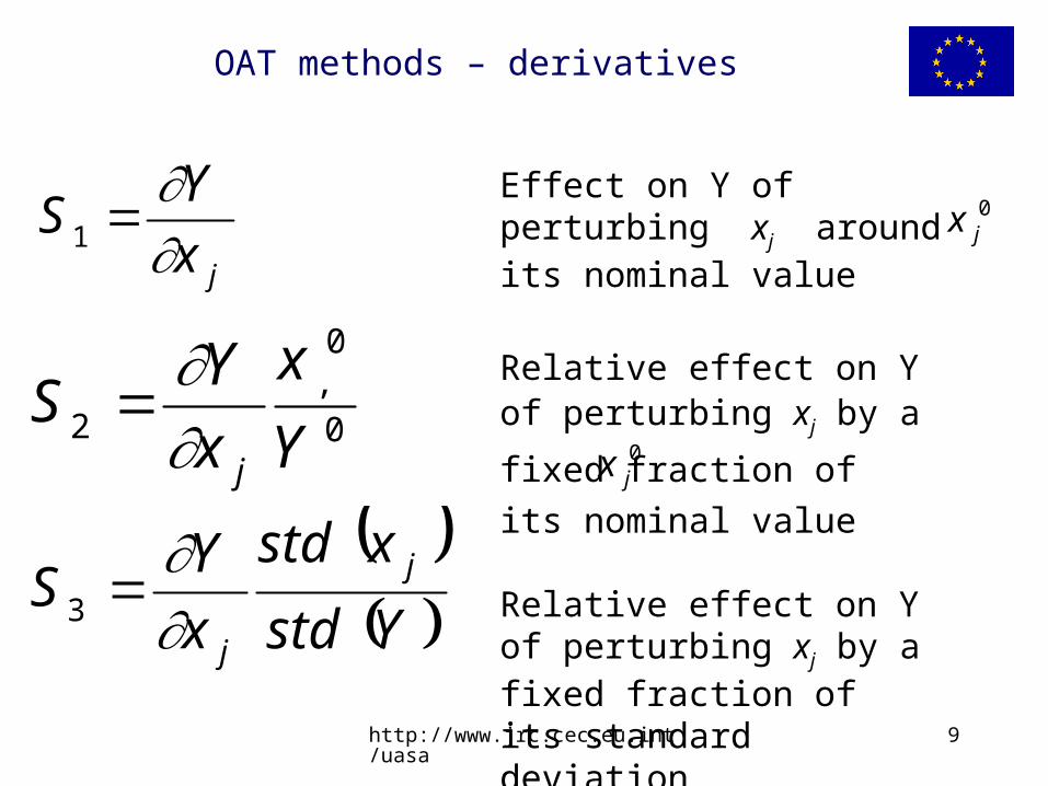
OAT methods – derivatives
jxY
S
1
0
0,
2 Y
x
xY
Sj
Ystd
xstd
xY
S j
j
3
Effect on Y of perturbing xj around its nominal value
Relative effect on Y of perturbing xj by a fixed
fraction of its nominal
value
Relative effect on Y of perturbing xj by a fixed fraction of its standard deviation
0jx
0jx
http://www.jrc.cec.eu.int/uasa 10
Derivatives can be computed efficiently using an array of different analytic, numeric or coding techniques (Turanyi and Rabitz 2000).
When coding methods are used, computer programmes are modified (e.g. inserting lines of code and coupling with libraries) so that derivatives of large set of variables can be automatically computed at runtime (Grievank, 2000; Cacuci, 2005).
OAT methods
http://www.jrc.cec.eu.int/uasa 11
While derivatives are valuable for an array of estimation, calibration, inverse problem solving, and related settings, their use in sensitivity analysis proper is modest in the presence of finite factors uncertainty and non linear models.
OAT methods
http://www.jrc.cec.eu.int/uasa 12
A search was made on January 2004 on Science Online, a companion web side of Science magazine (impact factor above 20!). All articles having “sensitivity analysis” as a keyword (23 in number) were reviewed.
All articles either presented what we would call an uncertainty analysis (assessing the uncertainty in Y) or performed an OAT type of sensitivity analysis.
OAT methods
http://www.jrc.cec.eu.int/uasa 13
Among practitioners of sensitivity analysis this is a known problem – non OAT approaches are considered too complex to be implemented by the majority of investigators.
Among the global methods used by informed practitioners are:
•variance based methods, already described, •the method of Morris, •various types of Monte Carlo filtering.
OAT methods
14
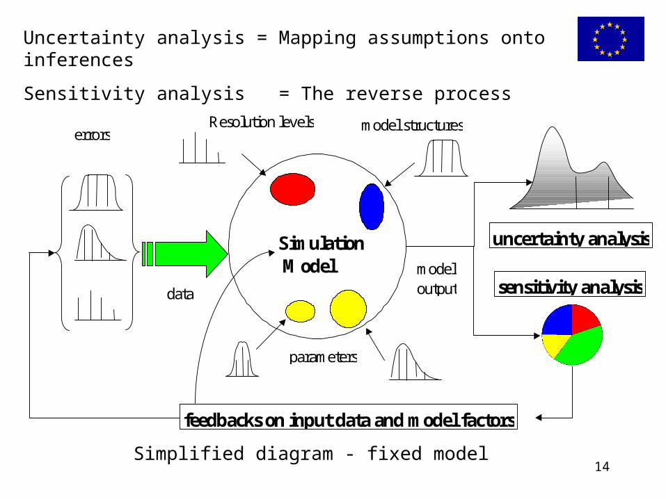
Uncertainty analysis = Mapping assumptions onto inferences
Sensitivity analysis = The reverse process
Simulation Model
parameters
Resolution levels
data
errorsmodel structures
uncertainty analysis
sensitivity analysismodel output
feedbacks on input data and model factors
Simplified diagram - fixed model
15
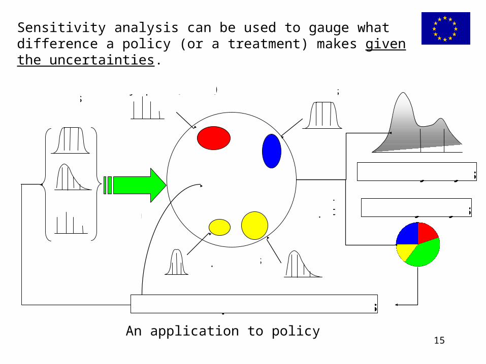
Sensitivity analysis can be used to gauge what difference a policy (or a treatment) makes given the uncertainties.
Simulation Model
parameters
Policy Options (latitude)
data
errorsmodel structures
uncertainty analysis
sensitivity analysismodel output
feedbacks on input data and model factors
An application to policy
http://www.jrc.cec.eu.int/uasa 16
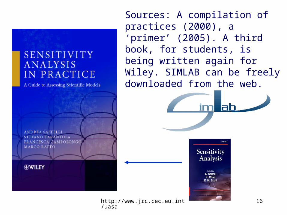
Sources: A compilation of practices (2000), a ‘primer’ (2005). A third book, for students, is being written again for Wiley. SIMLAB can be freely downloaded from the web.
http://www.jrc.cec.eu.int/uasa 17
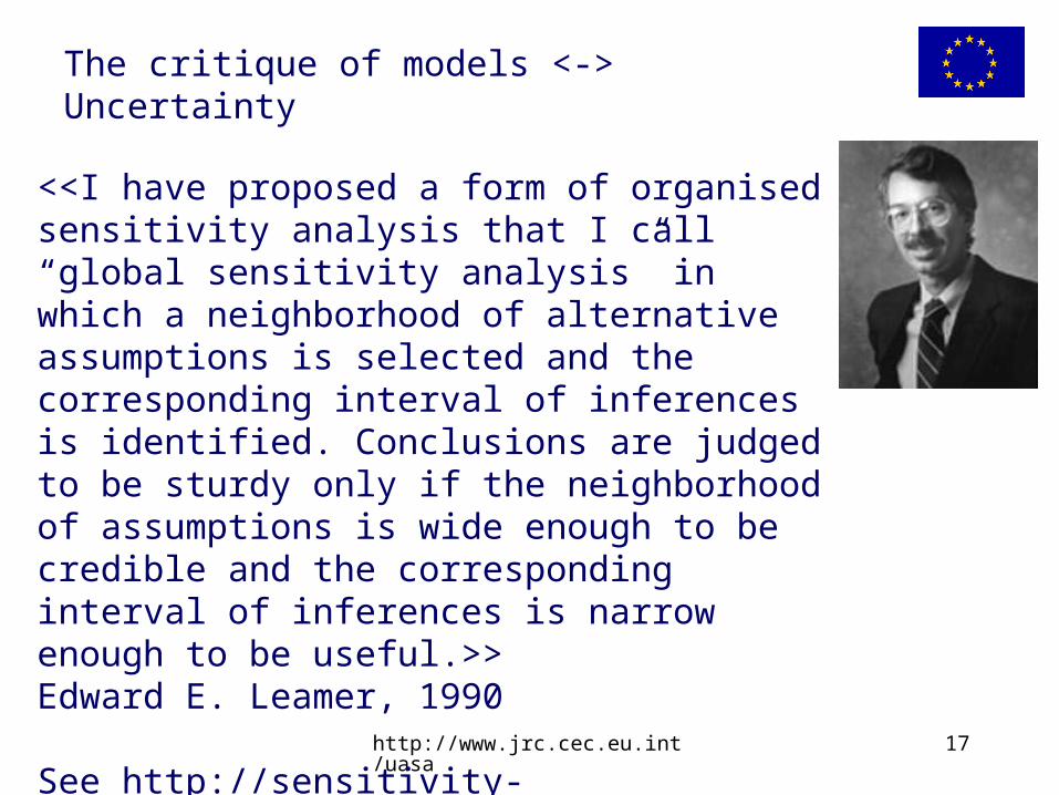
The critique of models <-> Uncertainty
<<I have proposed a form of organised sensitivity analysis that I call “global sensitivity analysis” in which a neighborhood of alternative assumptions is selected and the corresponding interval of inferences is identified. Conclusions are judged to be sturdy only if the neighborhood of assumptions is wide enough to be credible and the corresponding interval of inferences is narrow enough to be useful.>>Edward E. Leamer, 1990
See http://sensitivity-analysis.jrc.cec.eu.int/ for all references quoted in this talk.
http://www.jrc.cec.eu.int/uasa 18
Requirement 1. Focus About the output Y of interest.
The target of interest should not be the model output per se, but the question that the model has been called to answer. To make an example, if a model predicts contaminant distribution over space and time, it is the total area where a given threshold is exceeded at a given time which would play as output of interest, or the total health effects per time unit.
Our suggestions on useful requirements
http://www.jrc.cec.eu.int/uasa 19
… about the output Y of interest (continued)
One should seek from the analyses conclusions of relevance to the question put to the model, as opposed to relevant to the model, e.g.
•Uncertainty in emission inventories [in transport] are driven by variability in driving habits more than from uncertainty in engine emission data.
•In transport with chemical reaction problems, uncertainty in the chemistry dominates over uncertainty in the inventories.
Requirement 1 - Focus

http://www.jrc.cec.eu.int/uasa 20
A few words about the output Y of interest (continued)
•Engineered barrier count less than geologicalbarriers in radioactive waste migration.
Requirement 1 - Focus
http://www.jrc.cec.eu.int/uasa 21
On the output Y of interest(continued)
An implication of what just said is that models must change as the question put to them changes.
The optimality of a model must be weighted with respect to the task. According to Beck et al. 1997, a model is “relevant” when its input factors actually cause variation in the model response that is the object of the analysis.
Requirement 1 - Focus

http://www.jrc.cec.eu.int/uasa 22
Bruce Beck’s thought, continued
Model “un-relevance” could flag a bad model, or a model unnecessarily complex, used to fend off criticism from stakeholders (e.g. in environmental assessment studies). As an alternative, empirical model adequacy should be sought, especially when the model must be audited.
Requirement 1 - Focus
http://www.jrc.cec.eu.int/uasa 23
Requirement 2. Multidimensional averaging. In a sensitivity analysis all known sources of uncertainty should be explored simultaneously, to ensure that the space of the input uncertainties is thoroughly explored and that possible interactions are captured by the analysis. (as in EPA’s guidelines).
Requirements

http://www.jrc.cec.eu.int/uasa 24
Some of the uncertainties might be the result of a parametric estimation, but others may be linked to alternative formulations of the problems, or different framing assumptions which might reflect different views of reality, as well as different value judgements posed on it.
Requirement 2 – Multidimensional Averaging
http://www.jrc.cec.eu.int/uasa 25
Most models will be linear if one or few factors are changed in turn, and/or the range of variation is modest. Most models will be non linear and/or non additive otherwise.
Requirement 2 – Multidimensional Averaging
http://www.jrc.cec.eu.int/uasa 26
Typical non linear problems are multi-compartment or -phase, multi process models involving transfer of mass and/or energy, coupled with chemical reaction or transformation (e.g. filtration, decay…).
Our second requirement can also be formulated as: sensitivity analysis should work regardless of the properties of the model. It should be “model free”.
Requirement 2 – Multidimensional Averaging
http://www.jrc.cec.eu.int/uasa 27
Averaging across models.
When there are observations available to compute posterior probabilities on different plausible models, then sensitivity analysis should plug into a Bayesian model averaging.
Requirement 2 – Multidimensional Averaging
http://www.jrc.cec.eu.int/uasa 28
Requirement 3. Important how?. Another way for a sensitivity analysis to become irrelevant is to have different tests thrown at a problem, and different factors importance rankings produced without clue as to what to believe. To avoid this, a third requirement for sensitivity analysis is that the concept of importance be defined rigorously before the analysis.
Requirements
http://www.jrc.cec.eu.int/uasa 29
Requirement 4. Pareto. Most often input factors importance is distributed as wealth in nations, with few factors making all the uncertainty and most factors making a negligible contribution to it. A good method should do more than rank the factors, so that this Pareto effect, if present, can be revealed.
Requirement 5. Groups. When factors can be logically grouped in subsets, it is handy if the sensitivity measure can be computed for the group, with the same meaning as for the individual factor (as done by all speakers at this workshop when discussing variance based methods).
…
Requirements
http://www.jrc.cec.eu.int/uasa 30
Sensitivity analysis can
•surprise the analyst, •find technical errors, •gauge model adequacy and relevance,•identify critical regions in the space of the inputs (including interactions),•establish priorities for research, •simplify models,•verify if policy options (or treatments) make a difference or can be distinguished.•anticipate (prepare against) falsifications of the analysis •…
Incentives for sensitivity analysis
http://www.jrc.cec.eu.int/uasa 31
… there can be infinite applications as modelling setting are infinite. A model can be:
•Prognostic or diagnostic •Exploratory or consolidative (see Steven C. Bankes – ranging from an accurate predictor to a wild speculation) •Data driven (P. Young) or first-principle, i.e. parsimonious (usually to describe the past) or over-parametrised (to allow features of the future to emerge)•Disciplinary (physics, genetics, chemistry…) or statistical •Concerned with risk, control, optimisation, management, discovery, benchmark, didactic, …
Incentives for sensitivity analysis

http://www.jrc.cec.eu.int/uasa 32
What methods would meet these promises and fulfil our requirements?
The next section will try to introduce the methods, and some of their properties, using a very simple example.
Incentives for sensitivity analysis

http://www.jrc.cec.eu.int/uasa 33
Practices
We try to build a case for the use of a set of methods which in our experience met the requirements illustrated thus far. These are •Variance Based Methods •Morris method•Monte Carlo filtering and related measures

http://www.jrc.cec.eu.int/uasa 34
The first example introduces the variance based measures and the method of Morris.
35
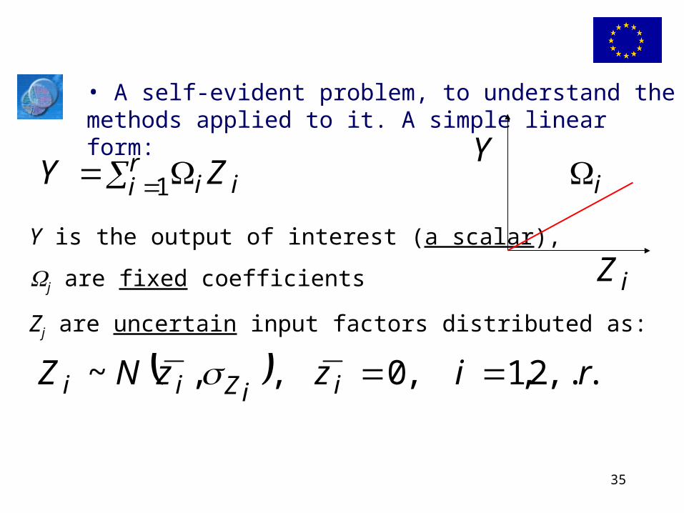
• A self-evident problem, to understand the methods applied to it. A simple linear form:
ri ii ZY 1
rizzNZ iiZii ,...,,,,~ 210
Y is the output of interest (a scalar),
j are fixed coefficients
Zj are uncertain input factors distributed as:
Y
iZ
i
36
ri ii ZY 1
Y
iZ
i
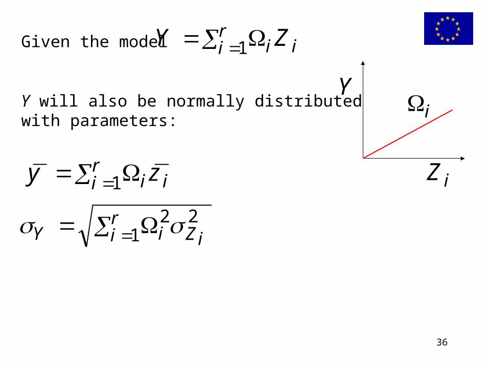
Given the model
Y will also be normally distributed with parameters:
ri ii zy 1
ri iZiY 1
22
37
ri ii ZY 1
Y
iZ
i
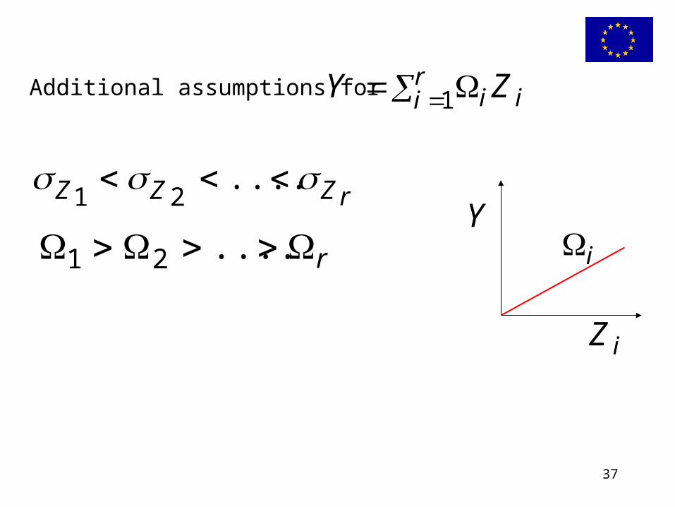
Additional assumptions for
rZZZ ....21
r ....21
http://www.jrc.cec.eu.int/uasa 38
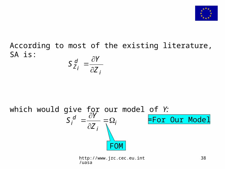
According to most of the existing literature, SA is:
which would give for our model of Y:
i
diZ Z
YS
ii
di Z
YS
FOM
=For Our Model
39
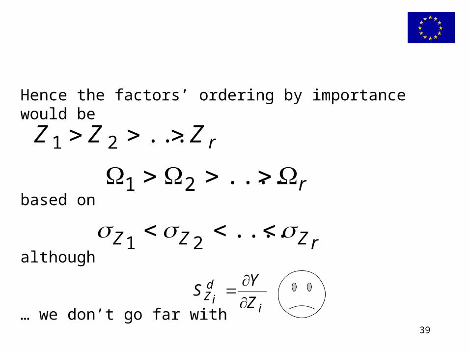
Hence the factors’ ordering by importance would be
based on
although
… we don’t go far with
rZZZ ...21
r ....21
rZZZ ....21
i
diZ Z
YS
http://www.jrc.cec.eu.int/uasa 40
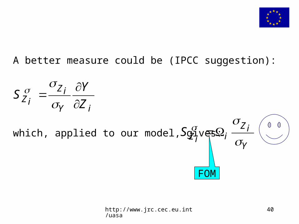
A better measure could be (IPCC suggestion):
which, applied to our model, gives:
iY
iZiZ Z
YS
Y
iZiiZS
FOM
41
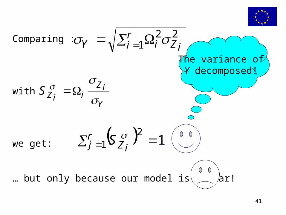
Comparing :
with
we get:
… but only because our model is linear!
Y
iZiiZS
ri iZiY 1
22
12
1 rj iZS
The variance of Y decomposed!
42
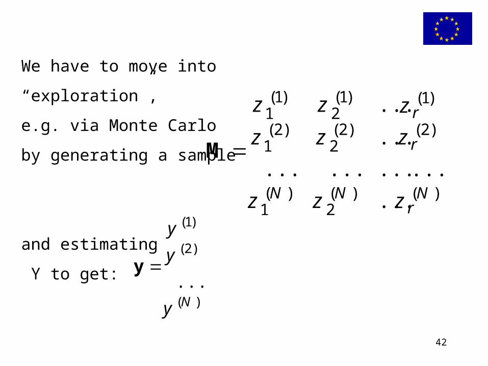
We have to move into
“exploration”,
e.g. via Monte Carlo
by generating a sample
and estimating
Y to get:
)(
)(
)(
)()(
)()(
)()(
...
...
.........
...
...
Nr
r
r
NN z
z
z
zz
zz
zz2
1
21
22
21
12
11
M
)(
)(
)(
...Ny
y
y2
1
y
http://www.jrc.cec.eu.int/uasa 43
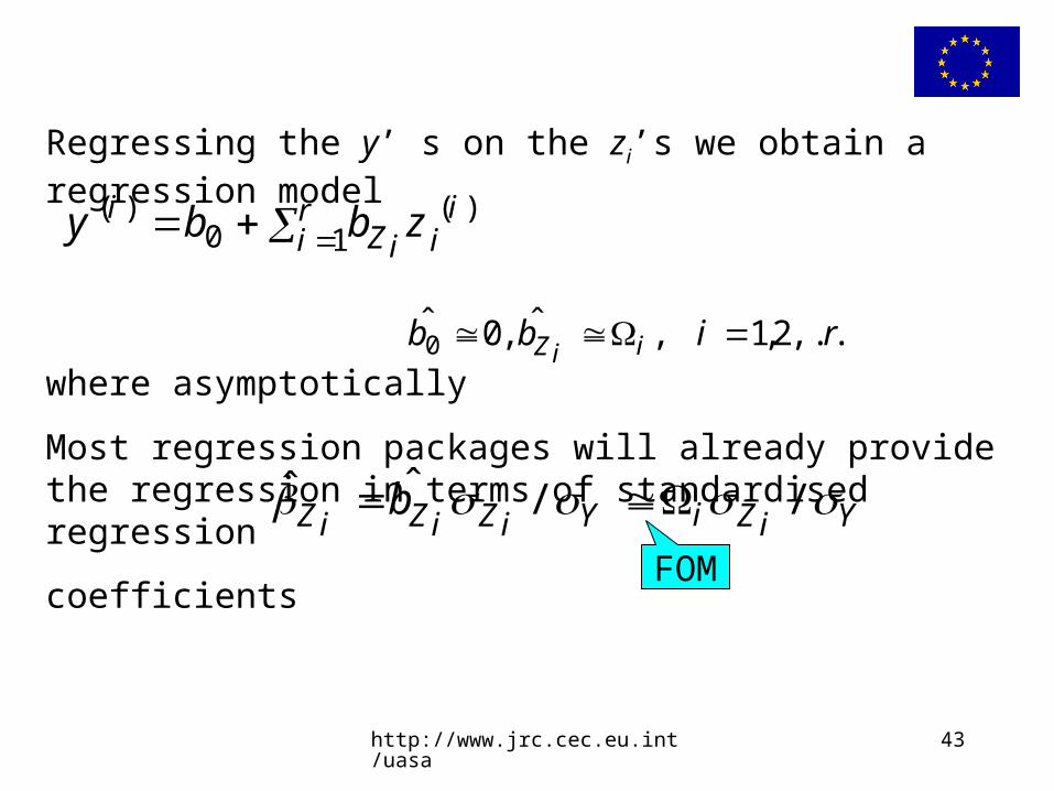
Regressing the y’ s on the zi’s we obtain a regression model
where asymptotically
Most regression packages will already provide the regression in terms of standardised regression
coefficients
)()( ii
ri iZ
i zbby 10
ribb iiZ ,...,,ˆ,ˆ 2100
YiZiYiZiZiZ b //ˆˆ
FOM
http://www.jrc.cec.eu.int/uasa 44
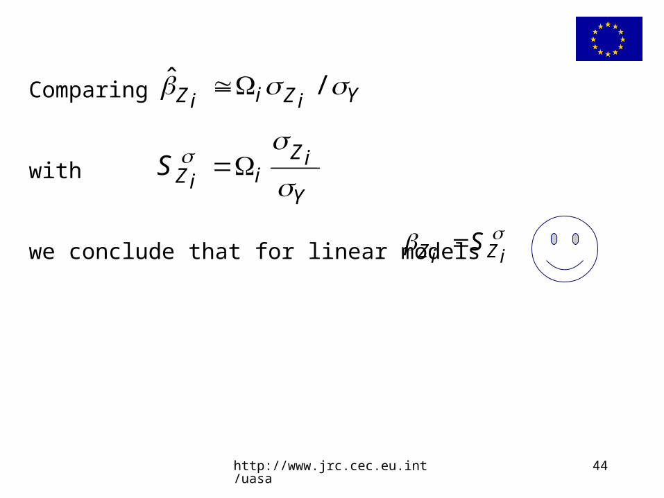
Comparing
with
we conclude that for linear models iZiZ S
YiZiiZ /ˆ
Y
iZiiZS
http://www.jrc.cec.eu.int/uasa 45
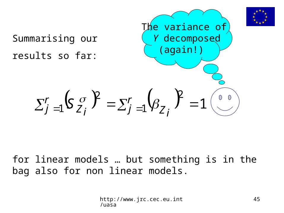
Summarising our
results so far:
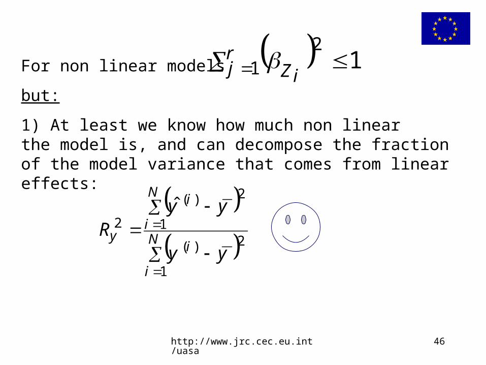
for linear models … but something is in the bag also for non linear models.
12
12
1 rj iZ
rj iZS
The variance of Y decomposed
(again!)
http://www.jrc.cec.eu.int/uasa 46
For non linear models
but:
1) At least we know how much non linear the model is, and can decompose the fractionof the model variance that comes from linear effects:
12
1 rj iZ
N
i
i
N
i
i
yyy
yyR
1
21
2
2
)(
)(ˆ
http://www.jrc.cec.eu.int/uasa 47
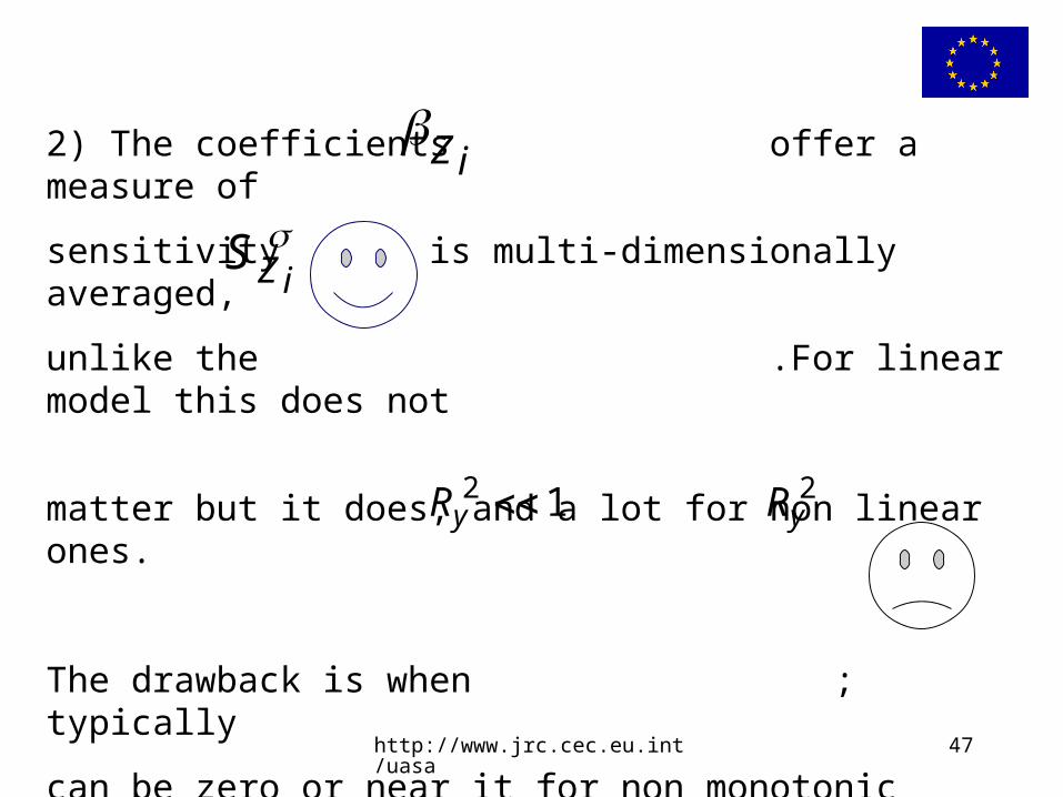
2) The coefficients offer a measure of
sensitivity that is multi-dimensionally averaged,
unlike the .For linear model this does not
matter but it does, and a lot for non linear ones.
The drawback is when ; typically
can be zero or near it for non monotonic models.
iZ
iZS
12 yR 2yR

http://www.jrc.cec.eu.int/uasa 48
Wrapping up the results so far obtained.
We like the idea of decomposing the variance of the model output of interest according to source (the input factors), but would like to do this for all models, independently from their degree of linearity or monotonicity. We would like a model-free approach.
http://www.jrc.cec.eu.int/uasa 49
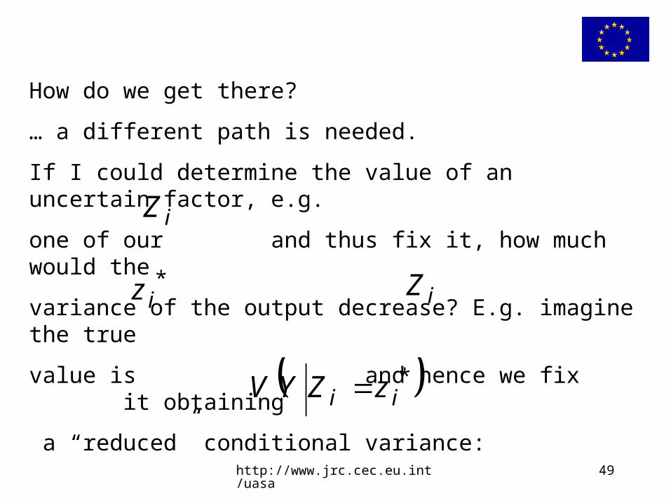
How do we get there?
… a different path is needed.
If I could determine the value of an uncertain factor, e.g.
one of our and thus fix it, how much would the
variance of the output decrease? E.g. imagine the true
value is and hence we fix it obtaining
a “reduced” conditional variance: *
ii zZYV
iZ
*iz iZ
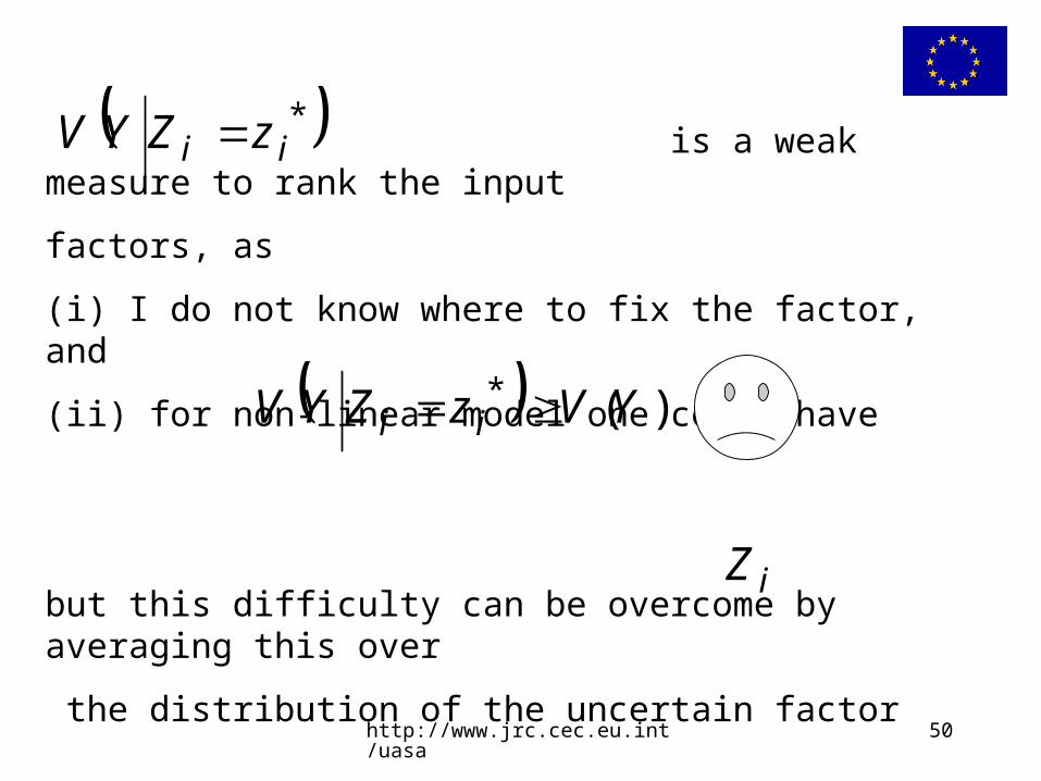
http://www.jrc.cec.eu.int/uasa 50
is a weak measure to rank the input
factors, as
(i) I do not know where to fix the factor, and
(ii) for non-linear model one could have
but this difficulty can be overcome by averaging this over
the distribution of the uncertain factor
)(* YVzZYV ii
*ii zZYV
iZ
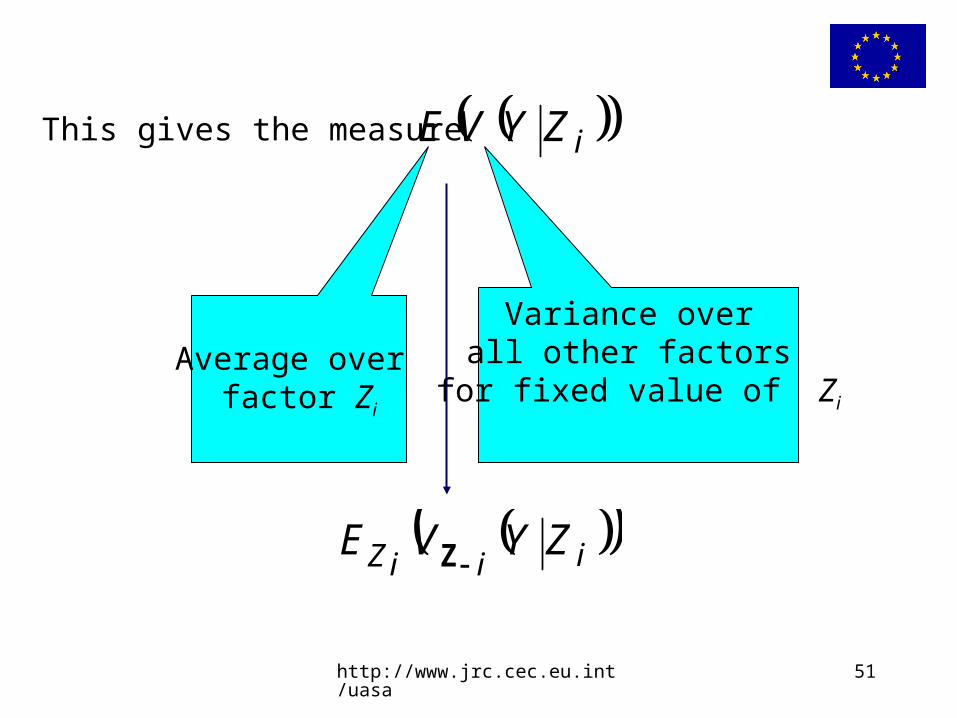
http://www.jrc.cec.eu.int/uasa 51
This gives the measure iZYVE
Average over factor Zi
Variance over all other factors
for fixed value of Zi
iiiZ ZYVEZ
http://www.jrc.cec.eu.int/uasa 52
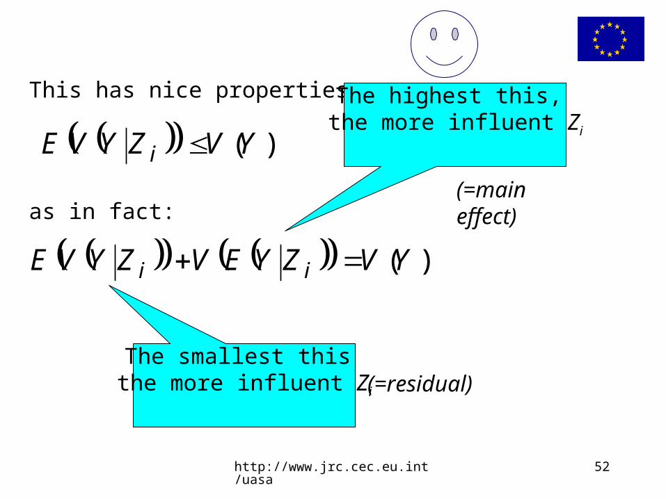
This has nice properties
as in fact:
)(YVZYVE i
)(YVZYEVZYVE ii
The smallest this the more influent Zi
The highest this, the more influent Zi
(=residual)
(=main effect)
http://www.jrc.cec.eu.int/uasa 53
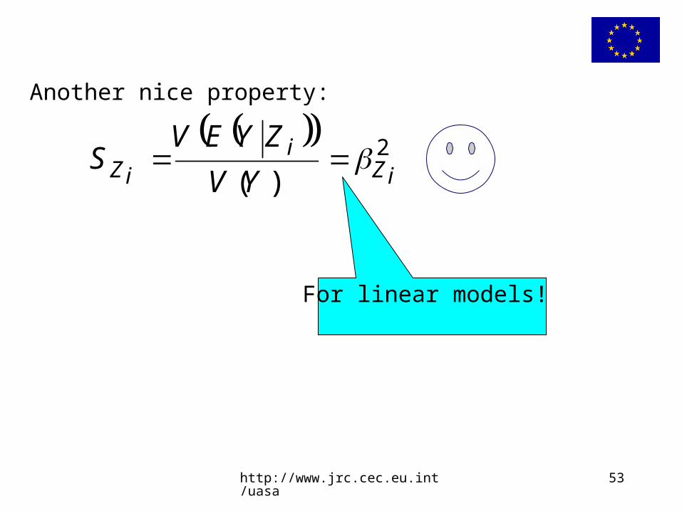
Another nice property:
2iZ
iiZ YV
ZYEVS
)(
For linear models!
http://www.jrc.cec.eu.int/uasa 54
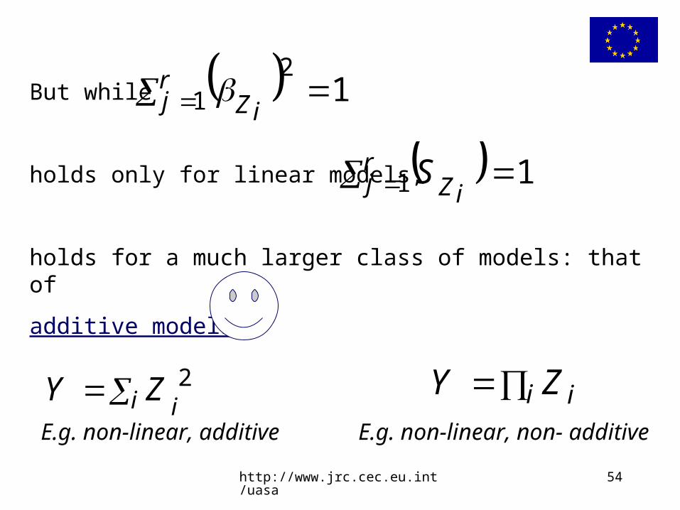
But while
holds only for linear models,
holds for a much larger class of models: that of
additive models.
12
1 rj iZ
11 rj iZS
i iZY 2 i iZY
E.g. non-linear, additive E.g. non-linear, non- additive
http://www.jrc.cec.eu.int/uasa 55
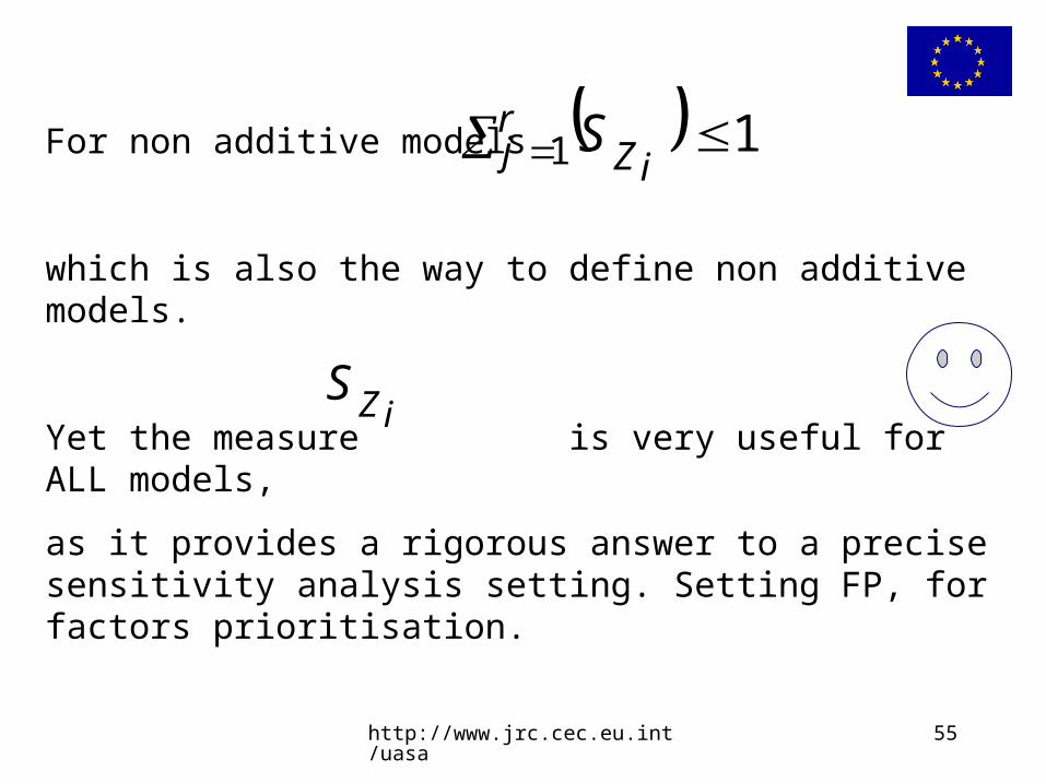
For non additive models
which is also the way to define non additive models.
Yet the measure is very useful for ALL models,
as it provides a rigorous answer to a precise sensitivity analysis setting. Setting FP, for factors prioritisation.
11 rj iZS
iZS
56
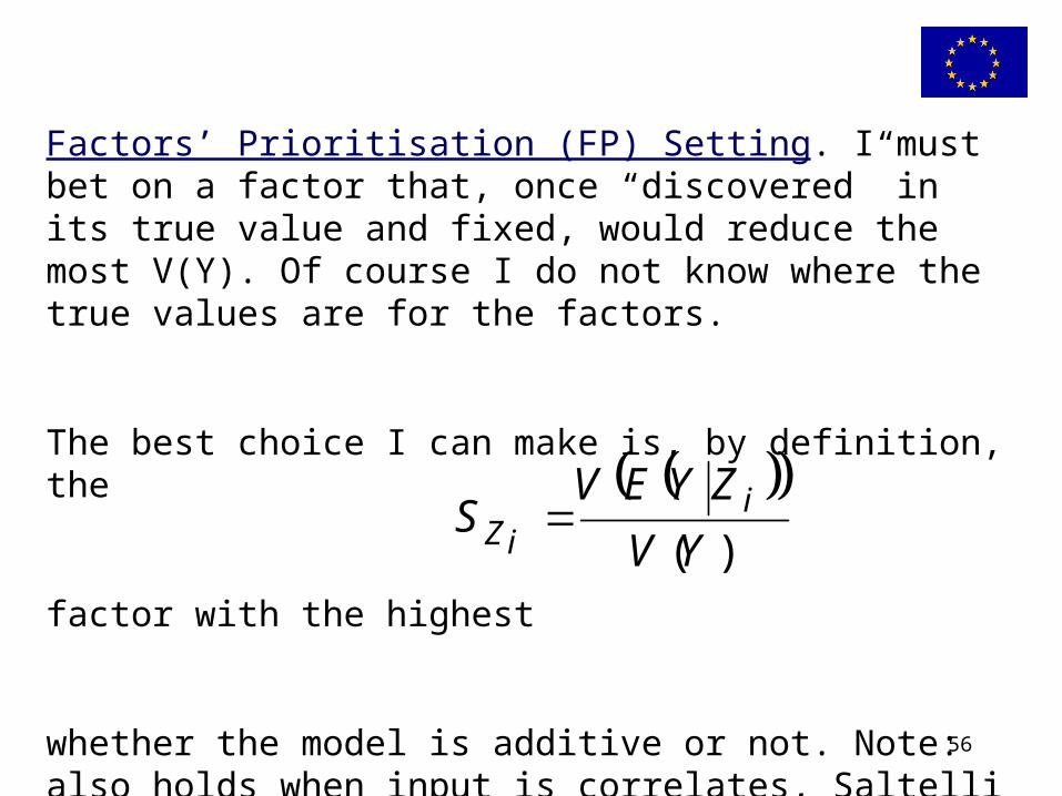
Factors’ Prioritisation (FP) Setting. I must bet on a factor that, once “discovered” in its true value and fixed, would reduce the most V(Y). Of course I do not know where the true values are for the factors.
The best choice I can make is, by definition, the
factor with the highest
whether the model is additive or not. Note: also holds when input is correlates, Saltelli and Tarantola, JASA 2002.
)(YV
ZYEVS i
iZ

http://www.jrc.cec.eu.int/uasa 57
To complete all this, we must say something about non additive model treatment, so let us complicate our model
by allowing both thej and Zj to be uncertain, i.e.
as before and riciN iiii ,...,, ,,~ 21
ri ii ZY 1
rizzNZ iiZii ,...,,,,~ 210
http://www.jrc.cec.eu.int/uasa 58
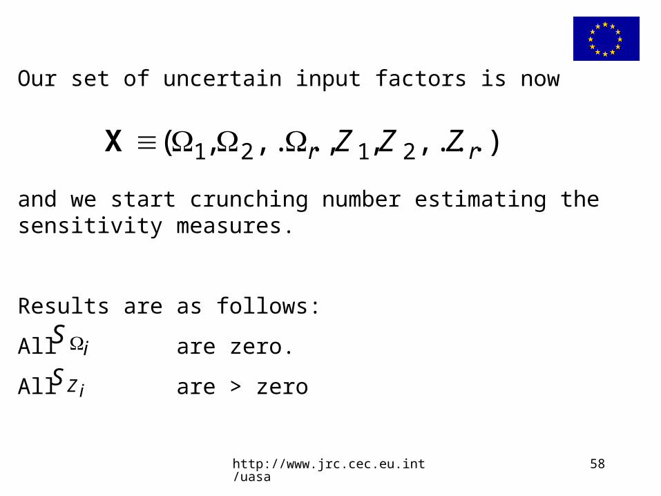
Our set of uncertain input factors is now
and we start crunching number estimating the sensitivity measures.
Results are as follows:
All are zero.
All are > zero
),...,,,...,( rr ZZZ 2121 X
iS
iZS
http://www.jrc.cec.eu.int/uasa 59
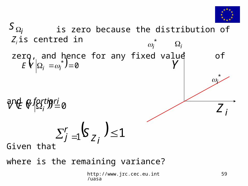
is zero because the distribution of Zi is centred in
zero, and hence for any fixed value of
and a fortiori
Given that
where is the remaining variance?
iS
0 *iiYE
*i i
0iYEV
11 rj iZS
Y
iZ
*i
http://www.jrc.cec.eu.int/uasa 60
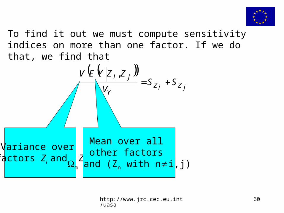
To find it out we must compute sensitivity indices on more than one factor. If we do that, we find that
jZiZ
Y
jiSS
V
ZZYEV
,
Variance over factors Zi and Zj
Mean over all other factors
m and (Zn with ni,j)
61
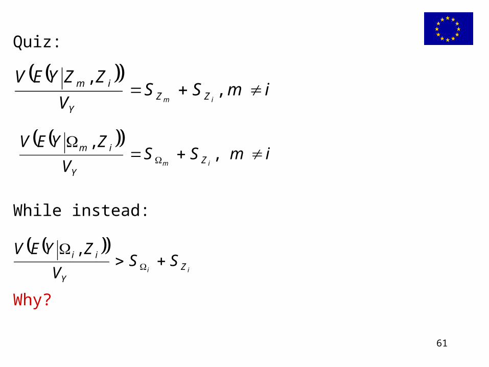
Quiz:
While instead:
Why?
ii Z
Y
ii SSV
ZYEV
,
imSS
V
ZZYEVim ZZ
Y
im ,,
imSS
V
ZYEVim Z
Y
im
,,
62
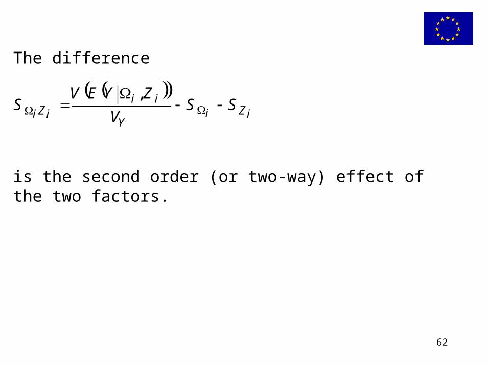
The difference
is the second order (or two-way) effect of the two factors.
iZi
Y
iiiZi
SSV
ZYEVS
,
http://www.jrc.cec.eu.int/uasa 63
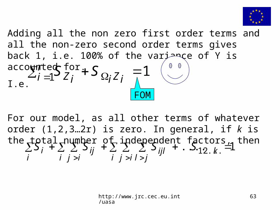
Adding all the non zero first order terms and all the non-zero second order terms gives back 1, i.e. 100% of the variance of Y is accounted for.
I.e.
For our model, as all other terms of whatever order (1,2,3…2r) is zero. In general, if k is the total number of independent factors, then
11 ri iZiiZ SS
i ij jl
kijli ij
iji
i SSSS 112.......
FOM
http://www.jrc.cec.eu.int/uasa 64
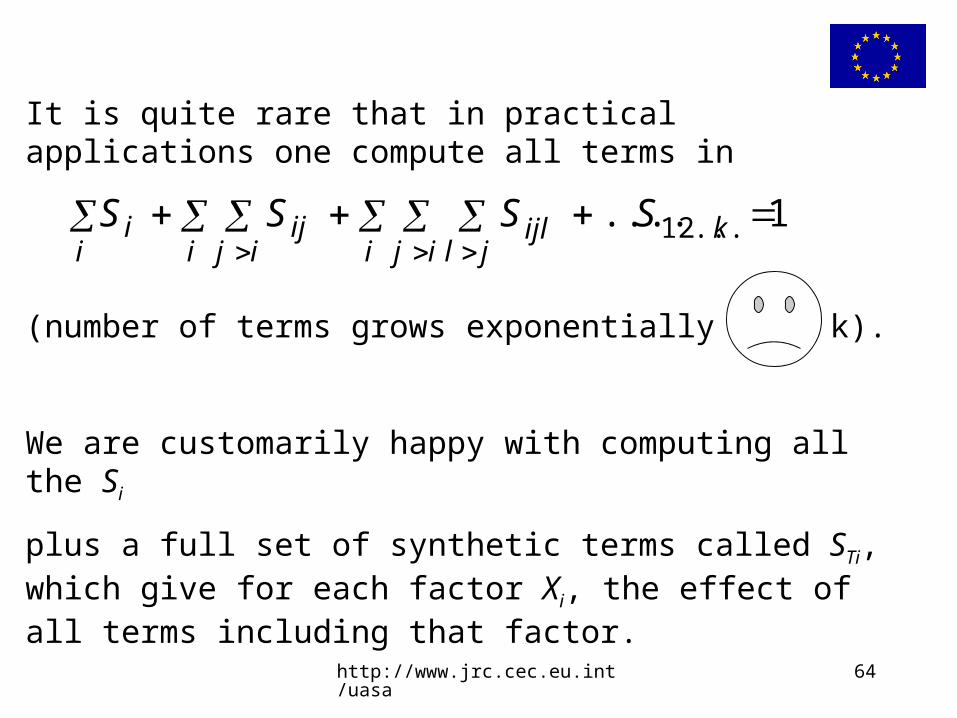
It is quite rare that in practical applications one compute all terms in
(number of terms grows exponentially with k).
We are customarily happy with computing all the Si
plus a full set of synthetic terms called STi, which give for each factor Xi, the effect of all terms including that factor.
i ij jl
kijli ij
iji
i SSSS 112.......
65
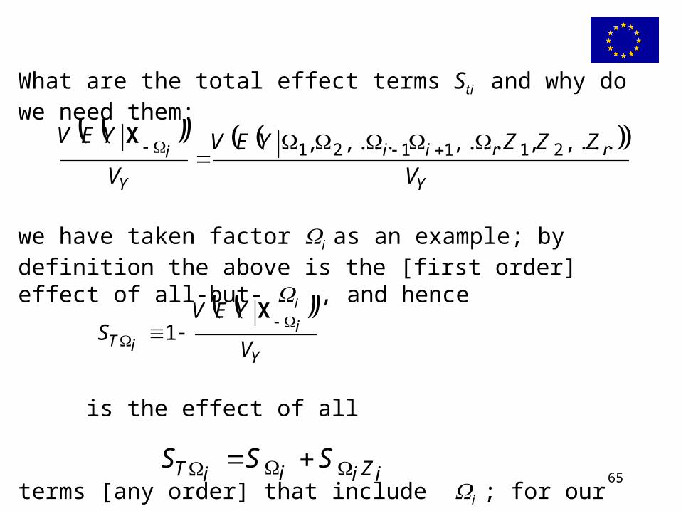
What are the total effect terms Sti and why do we need them:
we have taken factor i as an example; by definition the above is the [first order] effect of all-but- i , and hence
is the effect of all
terms [any order] that include i ; for our model
this is simply
Y
rrii
Y
i
V
ZZZYEV
V
YEV ,...,,...,..., 211121 X
Y
iiT V
YEVS
X1
iZiiiT SSS
66
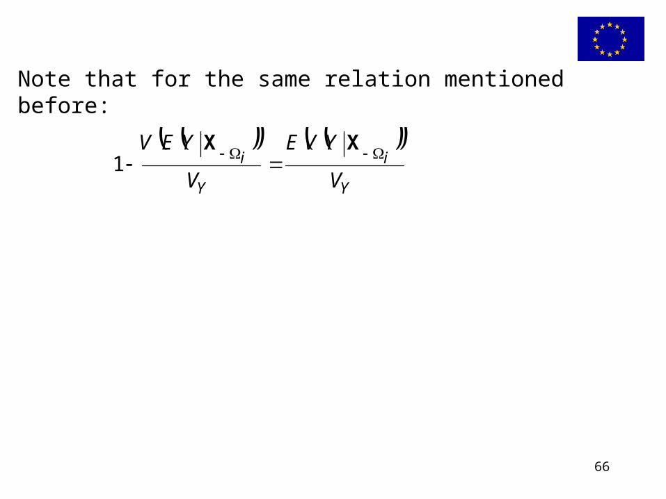
Note that for the same relation mentioned before:
Y
i
Y
i
V
YVE
V
YEV XX
1
http://www.jrc.cec.eu.int/uasa 67
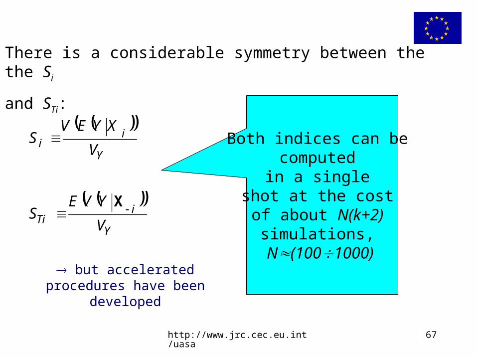
There is a considerable symmetry between the the Si
and STi:
Y
iTi V
YVES
X
Y
ii V
XYEVS Both indices can be
computed in a single
shot at the cost of about N(k+2)
simulations, N(1001000)
but accelerated procedures have been developed
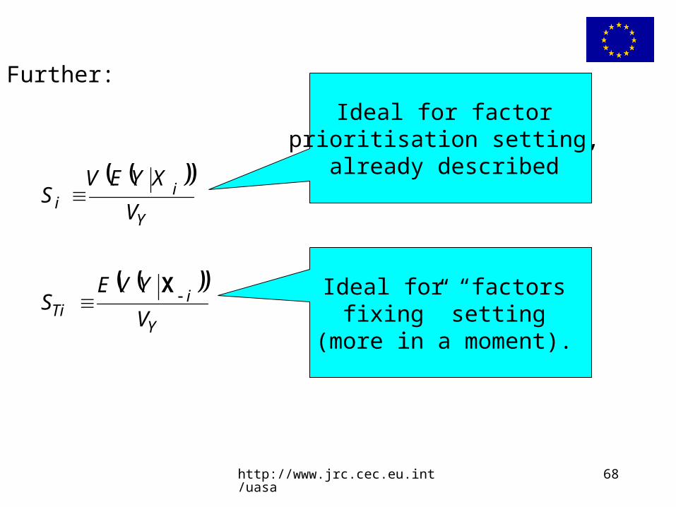
http://www.jrc.cec.eu.int/uasa 68
Further:
Y
iTi V
YVES
X
Y
ii V
XYEVS
Ideal for factor prioritisation setting,
already described
Ideal for “factors fixing” setting
(more in a moment).
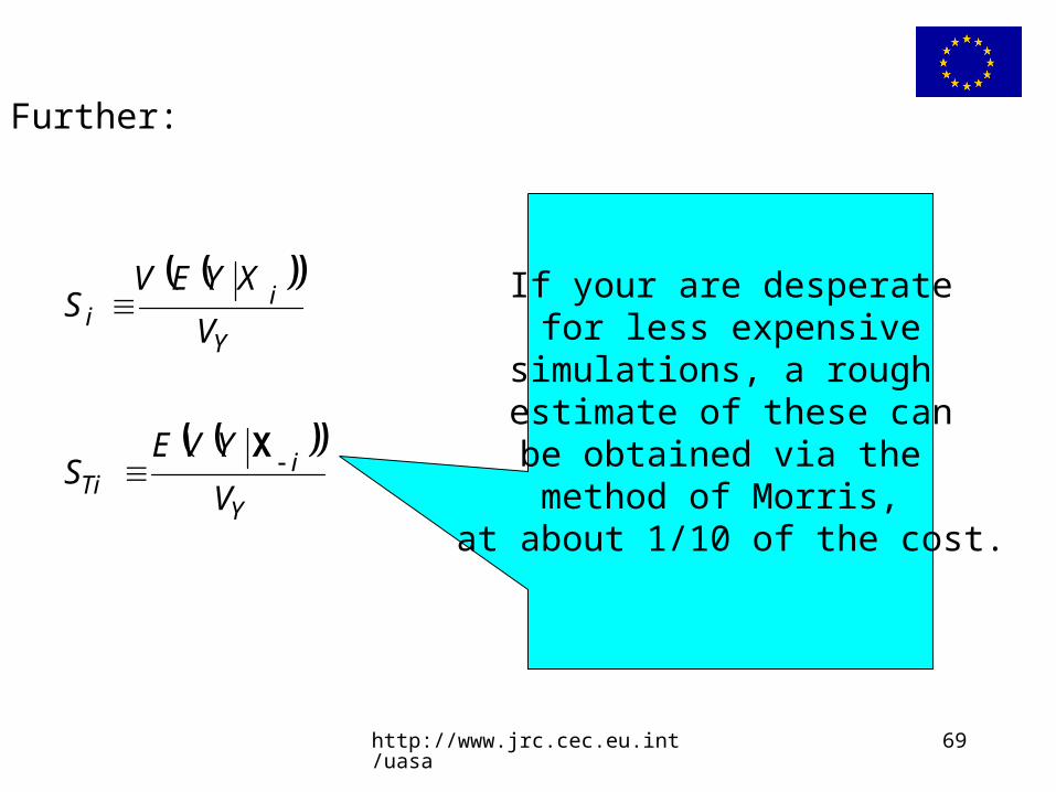
http://www.jrc.cec.eu.int/uasa 69
Further:
Y
iTi V
YVES
X
Y
ii V
XYEVS If your are desperate
for less expensive simulations, a rough estimate of these canbe obtained via the method of Morris,
at about 1/10 of the cost.
http://www.jrc.cec.eu.int/uasa 70
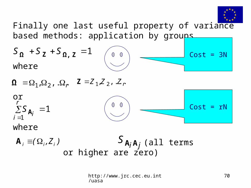
Finally one last useful property of variance based methods: application by groups.
where
or
where
(all terms or higher are zero)
1 ZΩ,ZΩ SSS
r ,..., 21Ω rZZZ ,..., 21Z
11
r
ii
SA
)Z,( iii A jiS AA
Cost = 3N
Cost = rN

http://www.jrc.cec.eu.int/uasa 71
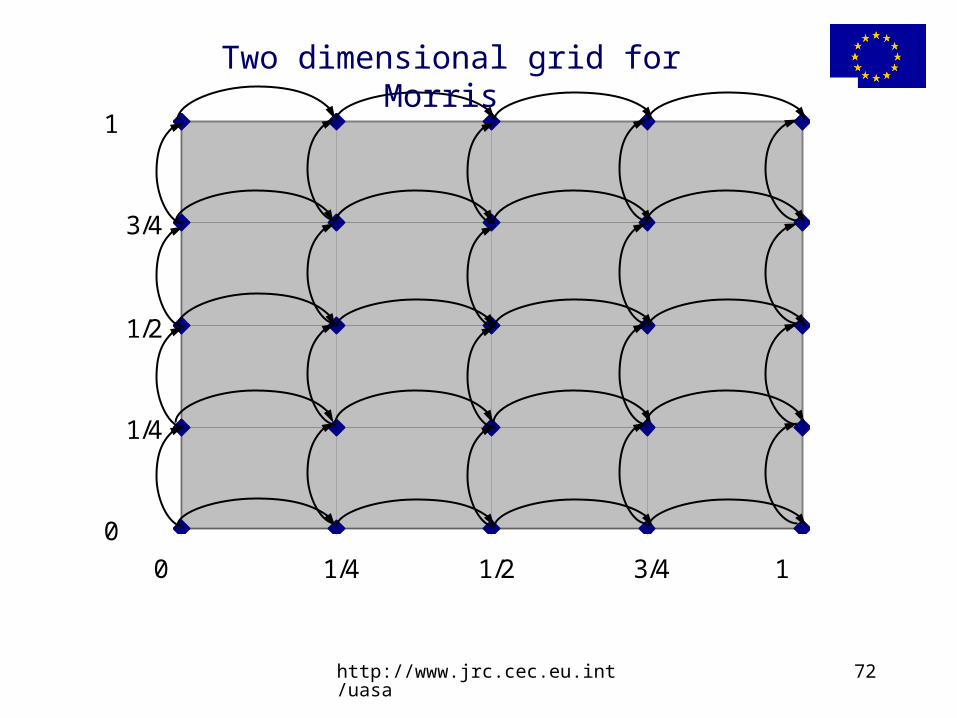
We mentioned the method of Morris – how does it work?
In brief, Morris is simply a derivative (in the form of an incremental ratios) computed at different point in the space of the input and averaged over the same space.
Hints about Morris
http://www.jrc.cec.eu.int/uasa 72
0
1/4
1/2
3/4
1
0 1/4 1/2 3/4 1
Two dimensional grid for Morris

http://www.jrc.cec.eu.int/uasa 73
We compute modulus elementary effects
|(Y(X)-Y(X-i,Xi+Delta)|
(increment only one factor by one step keeping the others fixed)
We do this at different points in the grid and take their average. This is not the original version of the test but it is the one proven by practice to be the most effective.
Hints about Morris

http://www.jrc.cec.eu.int/uasa 74
The next example offers an illustration of Monte Carlo filtering.
The idea behind MC filtering is straightforward and has been used extensively by hydro-geologists. Its history can be tracked back to ….
In MC filtering one runs a Monte Carlo experiment producing realisations of the output of interests corresponding to different sampled points in the input factors space.
Hints about Monte Carlo filtering
http://www.jrc.cec.eu.int/uasa 75
Done this, one can ‘filter’ the realisations, e.g. elements of the Y vector, by for instance comparing them with some sort of evidence or plausibility (e.g. one may have a good reason to reject all negatives values of Y).
This will partition the vector Y into two subsets: that of the well behaved Yi and that of the misbehaving Yi.
The same will apply to the (marginal) distributions of each of the input factors.
Hints about Monte Carlo filtering
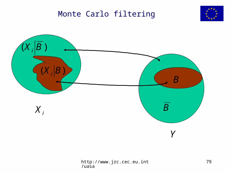
http://www.jrc.cec.eu.int/uasa 76
The input vector of each of the generic factors Xj explored in our experiments will result in a behaving subset Xij and a misbehaving Xij.
If the factor Xj is non influential in producing the [un] desired behaviour, than the two sub-samples will resample the original unfiltered sample of Xj.
Vice-versa, if the factor Xj is influential, than the two sub-samples will be different form one another as well as from the original unfiltered sample of Xj.
Hints about Monte Carlo filtering
http://www.jrc.cec.eu.int/uasa 77
Monte Carlo filtering
Summary of MC filtering, step by step:
•Define a range for k input factors Xi [1 < i < k], reflecting uncertainties in the model and make a number of Monte Carlo simulations. Each Monte Carlo simulation is associated to a vector of values of the input factors.
•Classify model outputs, according to the specification of the ‘acceptable’ model behaviour, [qualify a simulation as behaviour if the model output lies within constraints, non-behaviour otherwise]
BB
http://www.jrc.cec.eu.int/uasa 78
Monte Carlo filtering
Step by step:
Classifying simulations as either or , a set of binary elements is defined allowing to distinguish two
sub-sets for each Xi: of m elements and
of n elements [where n+m=N, the total number of Monte Carlo runs performed].
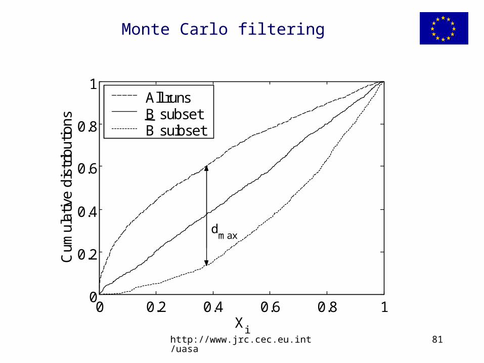
The Smirnov two-sample test (two-sided version) is performed for each factor independently, analyzing the maximum distance between the cumulative distributions of the and sets.
)( BX i
BB
)( BX i
B B
http://www.jrc.cec.eu.int/uasa 79
Monte Carlo filtering
)( BX i
iX
Y
)( BX i
B
B
http://www.jrc.cec.eu.int/uasa 80
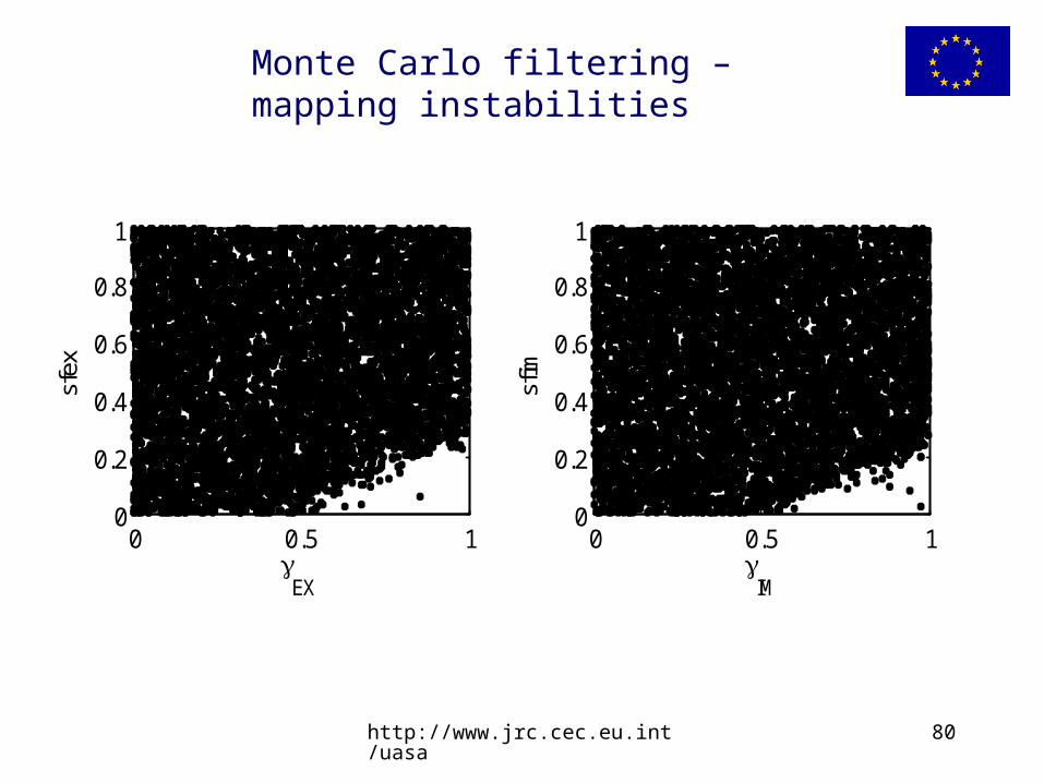
Monte Carlo filtering – mapping instabilities
0 0.5 10
0.2
0.4
0.6
0.8
1
IM
sfim
0 0.5 10
0.2
0.4
0.6
0.8
1
EX
sfex
http://www.jrc.cec.eu.int/uasa 81
Monte Carlo filtering
0 0.2 0.4 0.6 0.8 10
0.2
0.4
0.6
0.8
1
Xi
Cum
ulat
ive
dist
ribut
ions
All runsB subsetB suibset
dmax
http://www.jrc.cec.eu.int/uasa 82
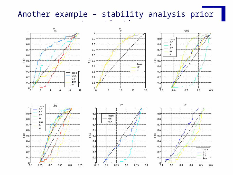
Another example – stability analysis prior to estimation
0 2 4 6 8 100
0.1
0.2
0.3
0.4
0.5
0.6
0.7
0.8
0.9
1
F(x
)
PX
baseGEXGIMinomX
0 5 10 15 200
0.1
0.2
0.3
0.4
0.5
0.6
0.7
0.8
0.9
1
F(x
)
W
baseW
0.5 0.6 0.7 0.8 0.90
0.1
0.2
0.3
0.4
0.5
0.6
0.7
0.8
0.9
1
F(x
)
habl
baseGCGLGYW
0.6 0.65 0.7 0.75 0.8 0.850
0.1
0.2
0.3
0.4
0.5
0.6
0.7
0.8
0.9
1
F(x
)
ilagbaseGCGIGYW
inomC
M
0.1 0.2 0.3 0.4 0.5 0.60
0.1
0.2
0.3
0.4
0.5
0.6
0.7
0.8
0.9
1
F(x
)
C
baseGCGYinom
0.15 0.2 0.25 0.3 0.35 0.40
0.1
0.2
0.3
0.4
0.5
0.6
0.7
0.8
0.9
1
F(x
)
IM
baseGEGIM
http://www.jrc.cec.eu.int/uasa 83
No time for any of the above?
Maybe I have no time to code any of the methods described so far.
Is there a quick and robust (as opposed to quick and dirty) way to obtain a good understanding of the input – output relationship using simply input and output values?
In fact for models with non too many factors to be looked at, a simple X-Y scatterplot can tell most of the story.
84
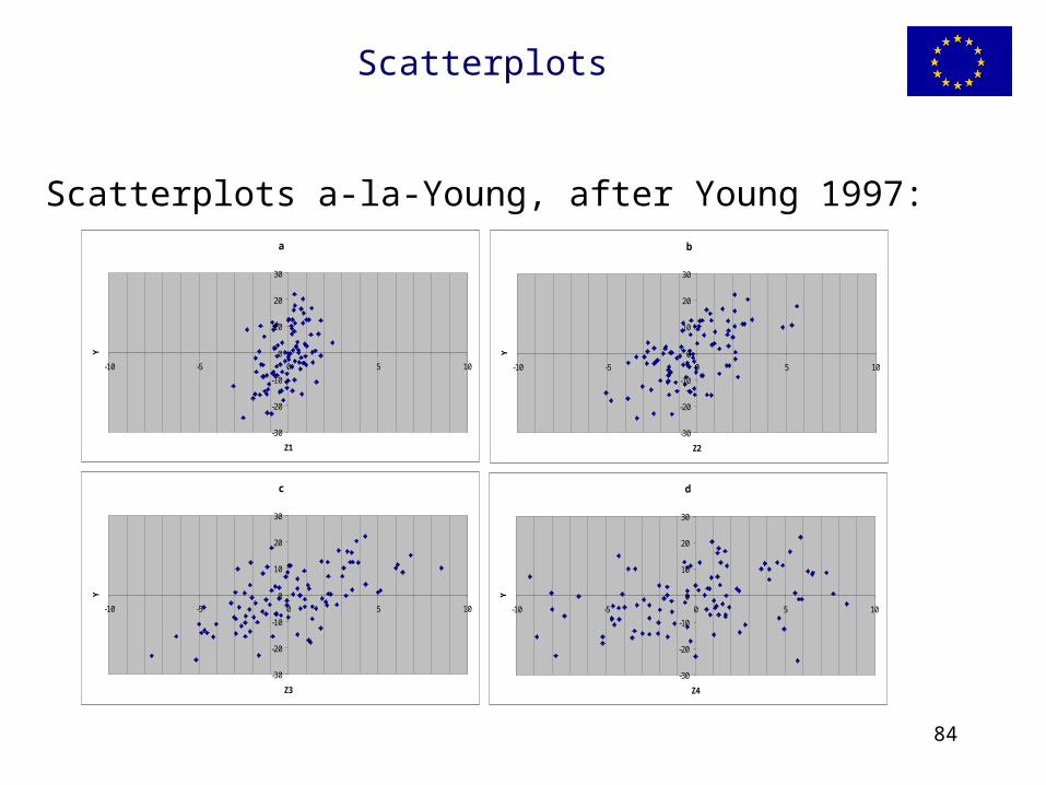
Scatterplots
Scatterplots a-la-Young, after Young 1997:
b
-30
-20
-10
0
10
20
30
-10 -5 0 5 10
Z2
Y
c
-30
-20
-10
0
10
20
30
-10 -5 0 5 10
Z3
Y
d
-30
-20
-10
0
10
20
30
-10 -5 0 5 10
Z4
Y
a
-30
-20
-10
0
10
20
30
-10 -5 0 5 10
Z1
Y

http://www.jrc.cec.eu.int/uasa 85
Scatterplots
If you look at the clouds, it will be intuitive that clouds with shapes (features) will be those of influential factors. Clouds with no shape will be those of non influential ones.
Another way of looking at those plots is to imagine to cut a vertical slice though each plot. Averaging all points on the slice will tell you the average value of Y at a fixed value of the point Xi. If this average changes moving about the Xi axis, then that factor is doing something.
http://www.jrc.cec.eu.int/uasa 86
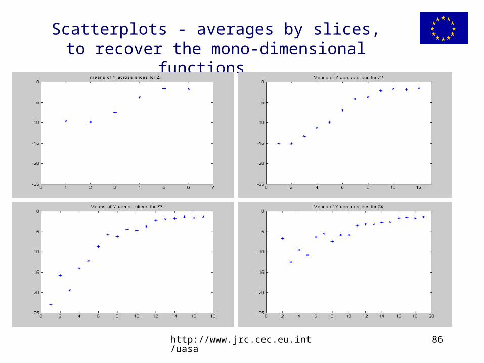
Scatterplots - averages by slices, to recover the mono-dimensional functions
http://www.jrc.cec.eu.int/uasa 87
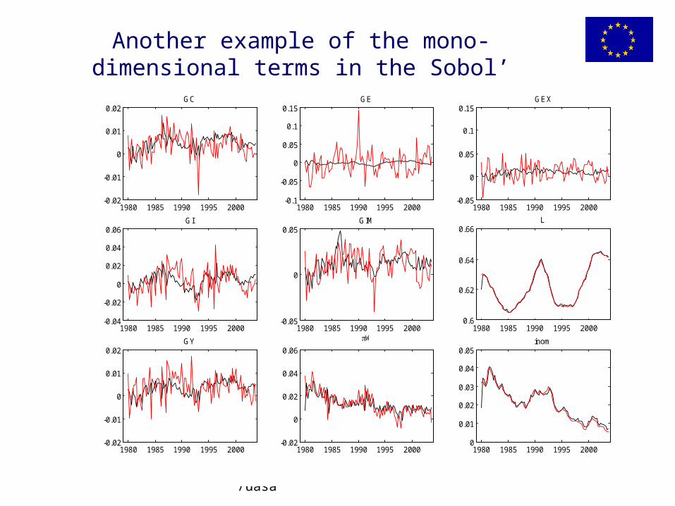
Another example of the mono-dimensional terms in the Sobol’ decomposition
1980 1985 1990 1995 2000-0.02
-0.01
0
0.01
0.02GC
1980 1985 1990 1995 2000-0.1
-0.05
0
0.05
0.1
0.15GE
1980 1985 1990 1995 2000-0.05
0
0.05
0.1
0.15GEX
1980 1985 1990 1995 2000-0.04
-0.02
0
0.02
0.04
0.06GI
1980 1985 1990 1995 2000-0.05
0
0.05GIM
1980 1985 1990 1995 20000.6
0.62
0.64
0.66L
1980 1985 1990 1995 2000-0.02
-0.01
0
0.01
0.02GY
1980 1985 1990 1995 2000-0.02
0
0.02
0.04
0.06
W
1980 1985 1990 1995 20000
0.01
0.02
0.03
0.04
0.05inom

http://www.jrc.cec.eu.int/uasa 88
Scatterplots
If V(E(Y|Xi) is high (over the slices), then Xi is doing something.
We have re-discovered the first order effect.
http://www.jrc.cec.eu.int/uasa 89
Scatterplots
In fact, instead of looking at the clouds, I can look at theses moving averages instead. This was done by practitioners such as Sacks, Welch and co-authors in the late 80’s - early 90’s.
Sacks et al., 1989, suggest a method of sensitivity analysis that is based on decomposing Y into terms (functions) of increasing dimensionality, and look at these as measure of sensitivity (see also an application in Welch et al., 1992).
http://www.jrc.cec.eu.int/uasa 90
Scatterplots – regression
Even better, if we manage to interpolate across these data clouds to yield robust estimates of E(Y|Xi). In fact today we do just that using modern interpolation methods derived by time series analysis (state dependent methods).
We then used a ‘rich’ sample of estimated E(Y|Xi) to compute the first order indices, i.e. V(E(Y|Xi))/V(Y).
http://www.jrc.cec.eu.int/uasa 91
Scatterplots – MC filtering
Scatterplots and Monte Carlo filtering can also be used in tandem – I can look at filtered plus unfiltered scatterplot of Y versus Xi to gain insight on the effect of Xi on Y in the behavioural runs (also in 2D).
Instead of filtering, I can also take a measure Z of the agreement between Y and observations (e.g. a likelihood) and compute V(E(Z|Xi)) , Sensitivity analysis for calibration.
http://www.jrc.cec.eu.int/uasa 92
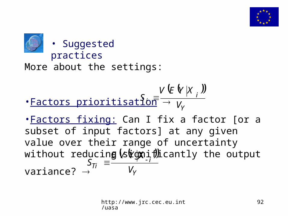
More about the settings:
•Factors prioritisation
•Factors fixing: Can I fix a factor [or a subset of input factors] at any given value over their range of uncertainty without reducing significantly the output
variance?
Y
ii V
XYEVS
Y
iTi V
YVES
X
• Suggested practices
http://www.jrc.cec.eu.int/uasa 93
More about the settings (continued):
•Factors mapping: Which factor is mostly responsible for producing realisations of Y in the region of interest? Monte Carlo Filtering and related tools (Ratto et al., 2000, 2005)
•Variance cutting: Reducing the variance of the output of a prescribed amount fixing the smallest number of factors… a combination of Si and Sti.

http://www.jrc.cec.eu.int/uasa 94
Why do we need settings?
•One way in which a SA can go wrong is because its purpose is left unspecified or vague (find the most important factors…). One throws different statistical tests and measures to the problem and obtains different factors rankings … then?
•Models can be audited and settings for sensitivity analysis can be audited as well.
Importance must be defined beforehand (Requirement Important how )

http://www.jrc.cec.eu.int/uasa 95
What else can go wrong in a sensitivity analysis?
•Too many outputs of interest - our initial discussion. What is the question? Is the model relevant to the question? See Beck et al. 1997 (Requirement Focus)
•Piecewise sensitivity (by sub-model, or one possible model at a time, or one factor at a time). Not only conflicts with the previous requirement but leads to a dangerously incomplete exploration of the uncertainties; interactions are overlooked. Plug all uncertainties is one shot (Requirement multidimensional averaging)
96
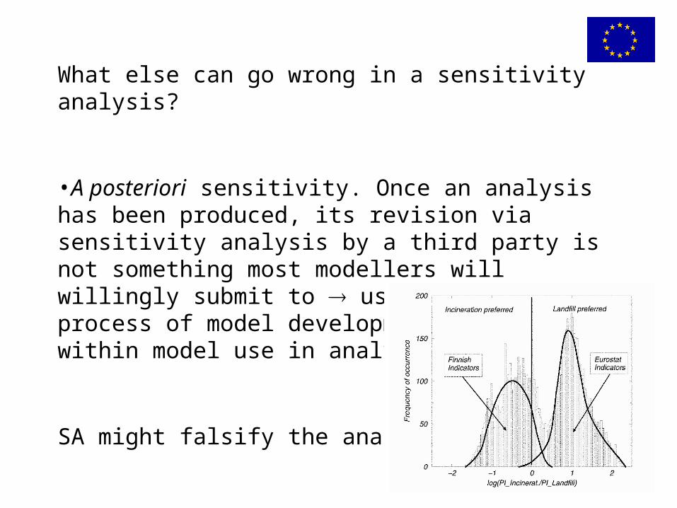
What else can go wrong in a sensitivity analysis?
•A posteriori sensitivity. Once an analysis has been produced, its revision via sensitivity analysis by a third party is not something most modellers will willingly submit to use SA in the process of model development, prior and within model use in analysis.
SA might falsify the analysis ...

http://www.jrc.cec.eu.int/uasa 97
Conclusions
•Increased need, scope and prescription for quantitative uncertainty and sensitivity analyses.
•Methods are mature for use, e.g. in terms of literature, software, computational cost, tested practice, ease of communication.
•Accelerated estimation procedures based on simulators, meta-models (RSM), such as those presented at this workshop appear very promising.
http://www.jrc.cec.eu.int/uasa 98
An set of presentations given at a recent school on SA, plus downloadable recent publications and software, can be found at:
http://sensitivity-analysis.jrc.cec.eu.int/
Saltelli, A., M. Ratto, S. Tarantola and F. Campolongo (2005) Sensitivity Analysis for Chemical Models, Chemical Reviews, 105(7) pp 2811 – 2828.
Free summer school in Venice, September 11-13 2006.
… and next SAMO will likely be in June 2007 in Budapest.

http://www.jrc.cec.eu.int/uasa 99
Petroleum System Modelling (viewgraphs are courtesy of ENI-AGIP, group of Paolo Ruffo, see
Ruffo et al. 2004)
http://www.jrc.cec.eu.int/uasa 100
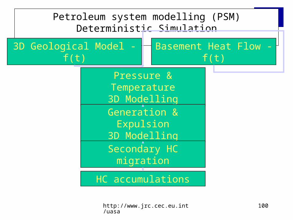
Petroleum system modelling (PSM) Deterministic Simulation
3D Geological Model - f(t) Basement Heat Flow - f(t)
Pressure & Temperature3D Modelling
Generation & Expulsion3D Modelling
Secondary HC migration
HC accumulations
http://www.jrc.cec.eu.int/uasa 101
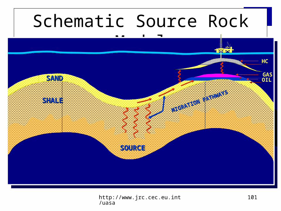
Schematic Source Rock Model
SHALESHALE
SOURCESOURCE
SANDSAND GASOIL
MIGRATION PATHWAYS
MIGRATION PATHWAYS
HC
http://www.jrc.cec.eu.int/uasa 102
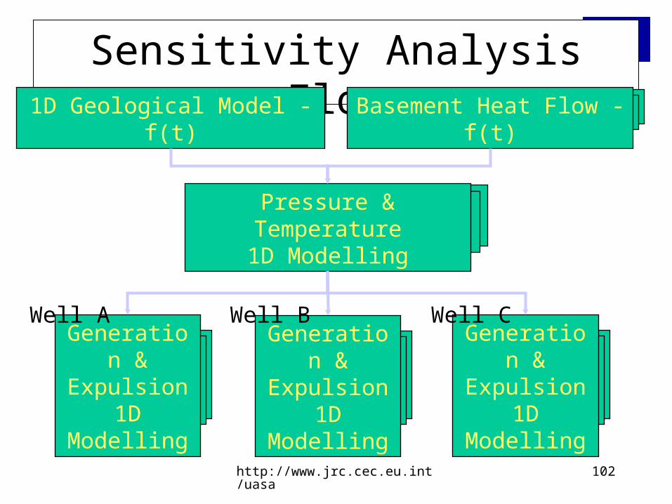
Sensitivity Analysis Flow
1D Geological Model - f(t)
Generation & Expulsion
1D Modelling
Well A
Basement Heat Flow - f(t)
Pressure & Temperature1D Modelling
Generation & Expulsion
1D Modelling
Well B
Generation & Expulsion
1D Modelling
Well C
http://www.jrc.cec.eu.int/uasa 103
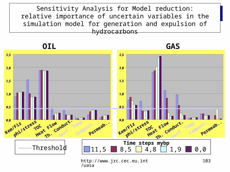
Sensitivity Analysis for Model reduction:relative importance of uncertain variables in the simulation model for
generation and expulsion of hydrocarbons
OIL GAS
ThresholdTime steps mybp
11,5 8,5 4,8 1,9 0,0
0,0
0,5
1,0
1,5
2,0
2,5
Kem/Fiz
phi/stres
s
TOC
Heat Flow
Th. Conduct.
Surf. Tem
p.
Compact.
Permeab..
0,0
0,5
1,0
1,5
2,0
2,5
Kem/Fiz
Compact.
phi/stres
sTOC
Heat Flow
Th. Conduct.
Surf. Tem
p.
Permeab..
http://www.jrc.cec.eu.int/uasa 104
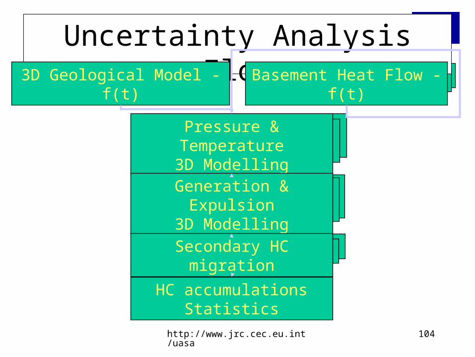
Uncertainty Analysis Flow
3D Geological Model - f(t) Basement Heat Flow - f(t)
Pressure & Temperature3D Modelling
Generation & Expulsion3D Modelling
Secondary HC migration
HC accumulations Statistics
http://www.jrc.cec.eu.int/uasa 105
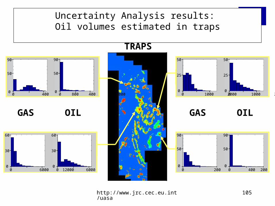
Uncertainty Analysis results: Oil volumes estimated in traps
TRAPS
60
30
0 0 6000 12000
60
30
0 0 6000 12000
50
25
0
50
25
0 0 1000 20000 1000 2000
90
50
0 0 200 400
90
50
0 0 200 400
GAS OIL GAS OIL
90
50
0 0 400 800 0 400 800
90
50
0
http://www.jrc.cec.eu.int/uasa 106
Conclusions
• The evaluation of the geological risk through a Probabilistic Petroleum System Modelling approach can be done combining Sensitivity and Uncertainty analyses.
• Sensitivity Analysis helps in reducing the number of parameters and particularly of scenarios.
• Uncertainty Analysis is usually based on a Monte Carlo approach: a sampling scheme can be used to reduce the number of runs.
• Calibration to experimental data, when available, can also help in reducing uncertainty ranges or even parameters/scenarios.


![Sensitivity analysis: An introduction - andrea saltelli · [Global*] sensitivity analysis: “The study of how the uncertainty in the output of a model (numerical or otherwise) can](https://img.pdfslide.us/doc/110x75/5e8c7fc23a7b6461e12bbfff/sensitivity-analysis-an-introduction-andrea-global-sensitivity-analysis-aoethe.jpg)