Semilinear parabolic partial differential equationsTheory, approximation, and applications

Stig Larsson

Chalmers University of Techology

Goteborg University

http://www.math.chalmers.se/˜stig

– p.1/65

Outline

Semilinear parabolic equation

Finite element method for elliptic equation

Finite element method for semilinear parabolic equation

Application to dynamical systems

Stochastic parabolic equation

Computer exercises with the software Puffin

– p.2/65

Lecture 1: Semilinear parabolic PDE

– p.3/65

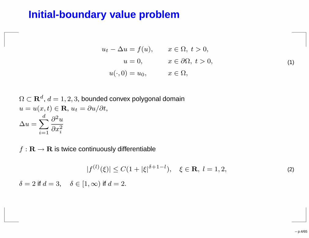
Initial-boundary value problem

ut − ∆u = f(u), x ∈ Ω, t > 0,

u = 0, x ∈ ∂Ω, t > 0,

u(·, 0) = u0, x ∈ Ω,

(1)

Ω ⊂ Rd, d = 1, 2, 3, bounded convex polygonal domain

u = u(x, t) ∈ R, ut = ∂u/∂t,

∆u =dX

i=1

∂2u

∂x2i

f : R → R is twice continuously differentiable

|f (l)(ξ)| ≤ C(1 + |ξ|δ+1−l), ξ ∈ R, l = 1, 2, (2)

δ = 2 if d = 3, δ ∈ [1,∞) if d = 2.

– p.4/65

Example: Allen-Cahn equation

f(ξ) = −V ′(ξ)

V (ξ) =1

4ξ4 −

1

2ξ2

ut − ∆u = −(u3 − u)

– p.5/65

Sobolev spaces

Hilbert space H = L2(Ω), with standard norm and inner product

‖v‖ =“

Z

Ω|v|2 dx

”1/2, (v,w) =

Z

Ωv · w dx. (3)

Sobolev spaces Hm(Ω), m ≥ 0, norms denoted by

‖v‖m =

X

|α|≤m

‖Dαv‖2

!1/2

. (4)

Hilbert space V = H10 (Ω), with norm ‖·‖1, the functions in H1(Ω) that vanish on ∂Ω.

V ∗ = H−1(Ω) is the dual space of V with norm

‖v‖−1 = supχ∈V

|(v, χ)|

‖χ‖1. (5)

– p.6/65

Sobolev spaces

X,Y Banach spacesL(X,Y ) denotes the space of bounded linear operators from X into YL(X) = L(X,X)

BX (x,R) denotes the closed ball in X with center x and radius R.BR = BV (0, R) denote the the closed ball of radius R in V :

BR = v ∈ V : ‖v‖1 ≤ R.

We also use the notation

‖v‖L∞([0,T ],X) = supt∈[0,T ]

‖v(t)‖X .

– p.7/65

Abstract framework

unbounded operator A = −∆ on Hdomain of definition D(A) = H2(Ω) ∩H1

0 (Ω)

A is a closed, densely defined, and self-adjoint positive definite operator in H with compactinverse.nonlinear operator f : V → H defined by f(v)(x) = f(v(x))

The initial-boundary value problem (??) may then be formulated as an initial value problem inV : find u(t) ∈ V such that

u′ +Au = f(u), t > 0; u(0) = u0. (6)

Eigenvalue problem:

Aϕ = λϕ

0 < λ1 < λ2 ≤ λ3 ≤ · · · ≤ λj → ∞

orthonormal basis of eigenvectors ϕj∞j=1

– p.8/65

Abstract framework

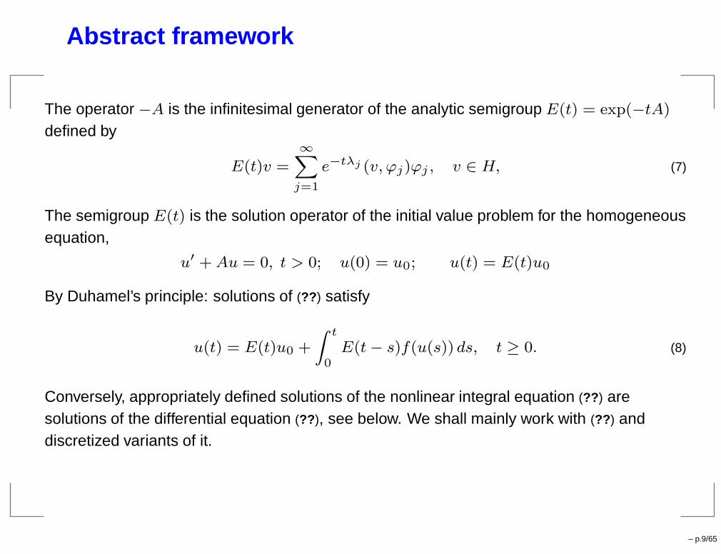
The operator −A is the infinitesimal generator of the analytic semigroup E(t) = exp(−tA)

defined by

E(t)v =∞X

j=1

e−tλj (v, ϕj)ϕj , v ∈ H, (7)

The semigroup E(t) is the solution operator of the initial value problem for the homogeneousequation,

u′ +Au = 0, t > 0; u(0) = u0; u(t) = E(t)u0

By Duhamel’s principle: solutions of (??) satisfy

u(t) = E(t)u0 +

Z t

0E(t− s)f(u(s)) ds, t ≥ 0. (8)

Conversely, appropriately defined solutions of the nonlinear integral equation (??) aresolutions of the differential equation (??), see below. We shall mainly work with (??) anddiscretized variants of it.

– p.9/65

Fractional powers of A

‖Aαv‖ =“

∞X

j=1

“

λαj (v, ϕj)

”2”1/2, α ∈ R,

D(Aα) =n

v : ‖Aαv‖ <∞o

, α ∈ R.

(9)

elliptic regularity estimate

‖v‖2 ≤ C‖Av‖, v ∈ H2(Ω) ∩H10 (Ω), (10)

trace inequality

‖v‖L2(∂Ω) ≤ C‖v‖1, v ∈ H1(Ω),

D(Al/2) = Hl(Ω) ∩H10 (Ω), l = 1, 2, with the equivalence of norms

c‖v‖l ≤ ‖Al/2v‖ ≤ C‖v‖l, v ∈ D(Al/2), l = 1, 2; (11)

D(A−1/2) = H−1(Ω)

c‖v‖−1 ≤ ‖A−1/2v‖ ≤ C‖v‖−1; (12)

– p.10/65

Analytic semigroup

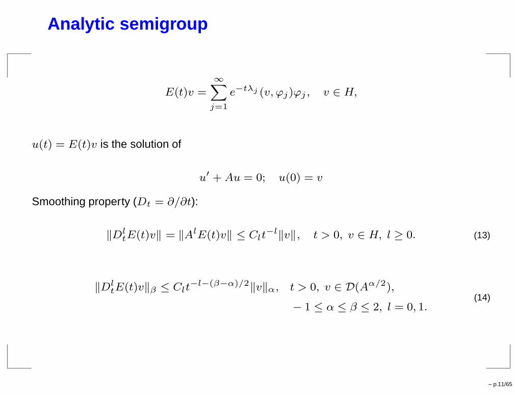
E(t)v =∞X

j=1

e−tλj (v, ϕj)ϕj , v ∈ H,

u(t) = E(t)v is the solution of

u′ +Au = 0; u(0) = v

Smoothing property (Dt = ∂/∂t):

‖DltE(t)v‖ = ‖AlE(t)v‖ ≤ Clt

−l‖v‖, t > 0, v ∈ H, l ≥ 0. (13)

‖DltE(t)v‖β ≤ Clt

−l−(β−α)/2‖v‖α, t > 0, v ∈ D(Aα/2),

− 1 ≤ α ≤ β ≤ 2, l = 0, 1.(14)

– p.11/65

Local Lipschitz condition

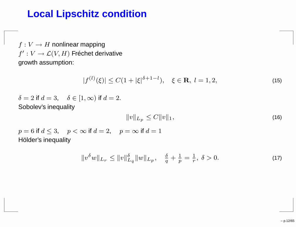
f : V → H nonlinear mappingf ′ : V → L(V,H) Fréchet derivativegrowth assumption:

|f (l)(ξ)| ≤ C(1 + |ξ|δ+1−l), ξ ∈ R, l = 1, 2, (15)

δ = 2 if d = 3, δ ∈ [1,∞) if d = 2.Sobolev’s inequality

‖v‖Lp≤ C‖v‖1, (16)

p = 6 if d ≤ 3, p <∞ if d = 2, p = ∞ if d = 1

Hölder’s inequality

‖vδw‖Lr≤ ‖v‖δ

Lq‖w‖Lp

, δq

+ 1p

= 1r, δ > 0. (17)

– p.12/65

Local Lipschitz condition

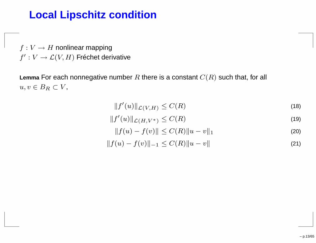
f : V → H nonlinear mappingf ′ : V → L(V,H) Fréchet derivative

Lemma For each nonnegative number R there is a constant C(R) such that, for allu, v ∈ BR ⊂ V ,

‖f ′(u)‖L(V,H) ≤ C(R) (18)

‖f ′(u)‖L(H,V ∗) ≤ C(R) (19)

‖f(u) − f(v)‖ ≤ C(R)‖u− v‖1 (20)

‖f(u) − f(v)‖−1 ≤ C(R)‖u− v‖ (21)

– p.13/65

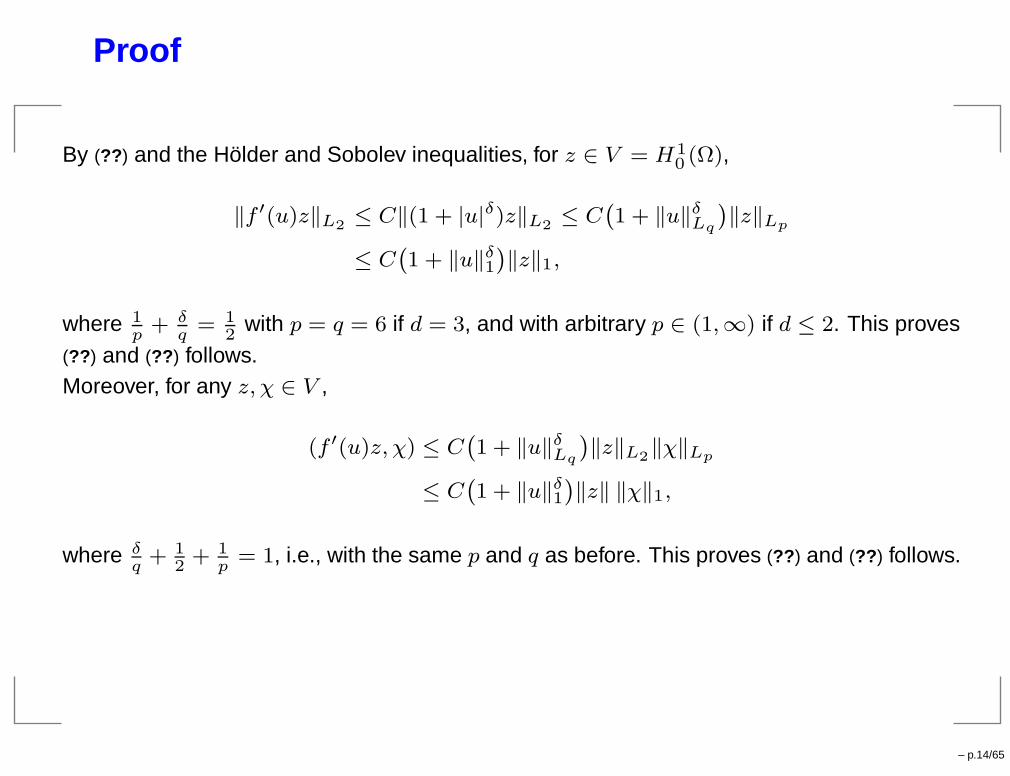
Proof

By (??) and the Hölder and Sobolev inequalities, for z ∈ V = H10 (Ω),

‖f ′(u)z‖L2≤ C‖(1 + |u|δ)z‖L2

≤ C`

1 + ‖u‖δLq

´

‖z‖Lp

≤ C`

1 + ‖u‖δ1

´

‖z‖1,

where 1p

+ δq

= 12

with p = q = 6 if d = 3, and with arbitrary p ∈ (1,∞) if d ≤ 2. This proves(??) and (??) follows.Moreover, for any z, χ ∈ V ,

(f ′(u)z, χ) ≤ C`

1 + ‖u‖δLq

´

‖z‖L2‖χ‖Lp

≤ C`

1 + ‖u‖δ1

´

‖z‖ ‖χ‖1,

where δq

+ 12

+ 1p

= 1, i.e., with the same p and q as before. This proves (??) and (??) follows.

– p.14/65

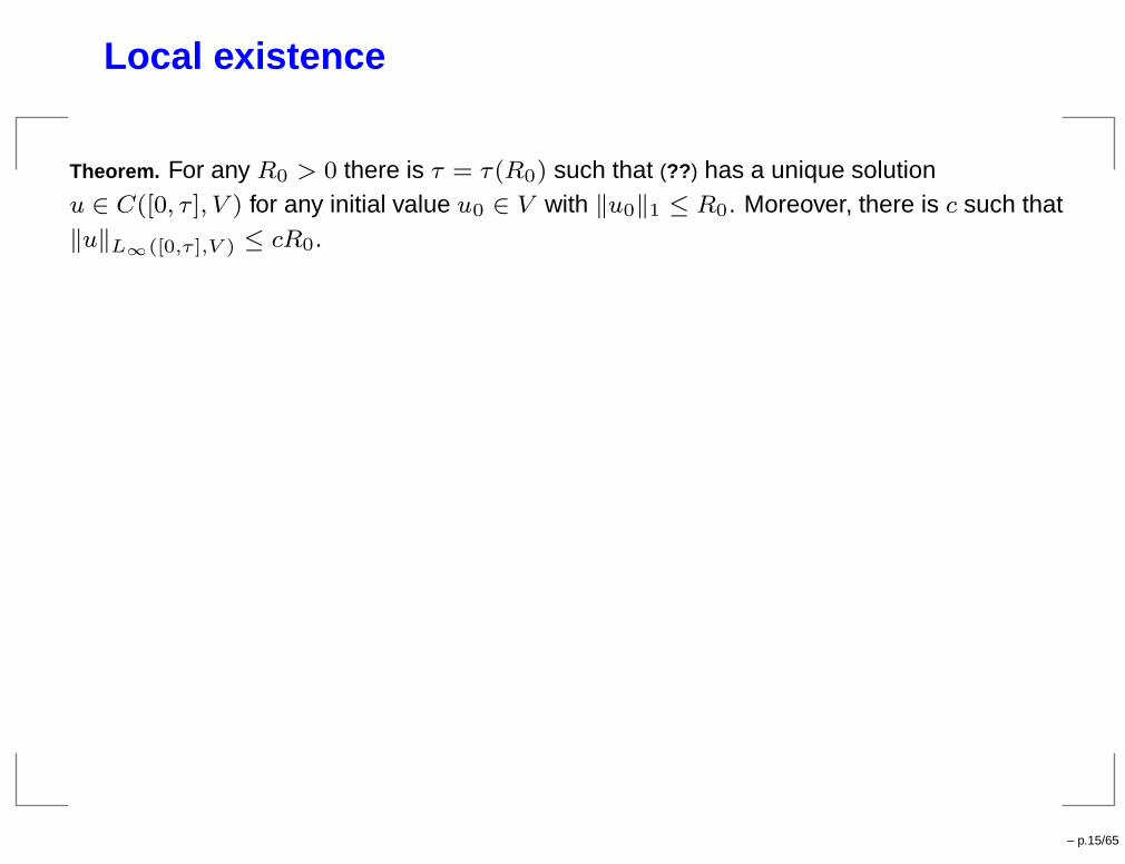
Local existence

Theorem. For any R0 > 0 there is τ = τ(R0) such that (??) has a unique solutionu ∈ C([0, τ ], V ) for any initial value u0 ∈ V with ‖u0‖1 ≤ R0. Moreover, there is c such that‖u‖L∞([0,τ ],V ) ≤ cR0.

– p.15/65

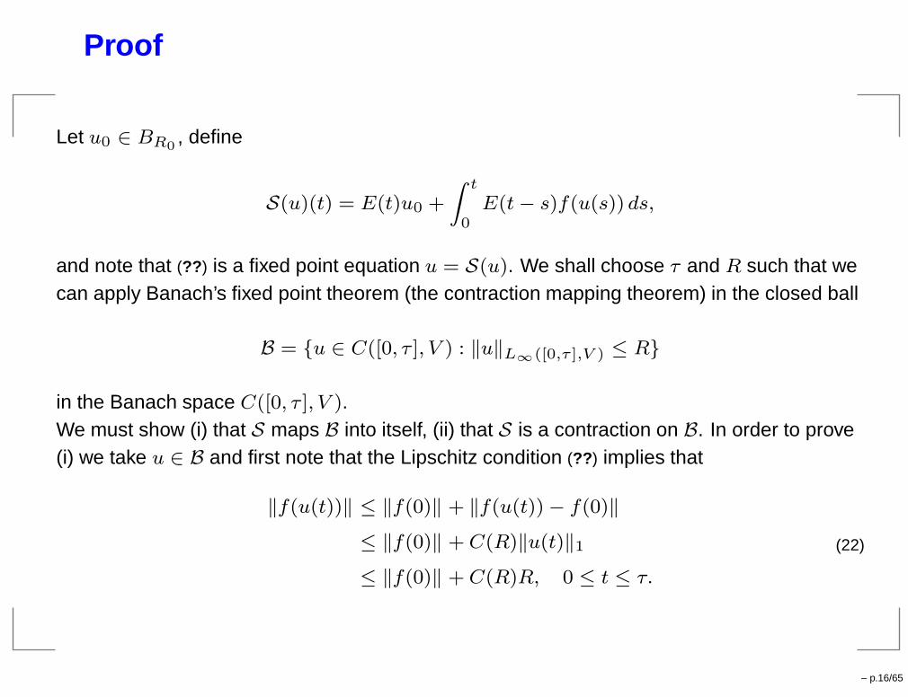
Proof

Let u0 ∈ BR0, define

S(u)(t) = E(t)u0 +

Z t

0E(t− s)f(u(s)) ds,

and note that (??) is a fixed point equation u = S(u). We shall choose τ and R such that wecan apply Banach’s fixed point theorem (the contraction mapping theorem) in the closed ball

B = u ∈ C([0, τ ], V ) : ‖u‖L∞([0,τ ],V ) ≤ R

in the Banach space C([0, τ ], V ).We must show (i) that S maps B into itself, (ii) that S is a contraction on B. In order to prove(i) we take u ∈ B and first note that the Lipschitz condition (??) implies that

‖f(u(t))‖ ≤ ‖f(0)‖ + ‖f(u(t)) − f(0)‖

≤ ‖f(0)‖ + C(R)‖u(t)‖1

≤ ‖f(0)‖ + C(R)R, 0 ≤ t ≤ τ.

(22)

– p.16/65

Proof, cont’d

Hence, using also (??), we get

‖S(u)(t)‖1 ≤ ‖E(t)u0‖1 +

Z t

0‖E(t− s)f(u(s))‖1 ds

≤ c0‖u0‖1 + c1

Z t

0(t− s)−1/2‖f(u(s))‖ ds

≤ c0R0 + 2c1τ1/2`

‖f(0)‖ + C(R)R´

, 0 ≤ t ≤ τ.

This implies

‖S(u)‖L∞([0,τ ],V ) ≤ c0R0 + 2c1τ1/2`

‖f(0)‖ + C(R)R´

.

Choose R = 2c0R0 and τ = τ(R0) so small that

2c1τ1/2`

‖f(0)‖ + C(R)R´

≤ 12R. (23)

Then ‖S(u)‖L∞([0,τ ],V ) ≤ R and we conclude that S maps B into itself.

– p.17/65

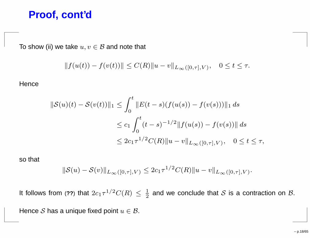
Proof, cont’d

To show (ii) we take u, v ∈ B and note that

‖f(u(t)) − f(v(t))‖ ≤ C(R)‖u− v‖L∞([0,τ ],V ), 0 ≤ t ≤ τ.

Hence

‖S(u)(t) − S(v(t))‖1 ≤

Z t

0‖E(t− s)(f(u(s)) − f(v(s)))‖1 ds

≤ c1

Z t

0(t− s)−1/2‖f(u(s)) − f(v(s))‖ ds

≤ 2c1τ1/2C(R)‖u− v‖L∞([0,τ ],V ), 0 ≤ t ≤ τ,

so that

‖S(u) − S(v)‖L∞([0,τ ],V ) ≤ 2c1τ1/2C(R)‖u− v‖L∞([0,τ ],V ).

It follows from (??) that 2c1τ1/2C(R) ≤ 12

and we conclude that S is a contraction on B.

Hence S has a unique fixed point u ∈ B.

– p.18/65

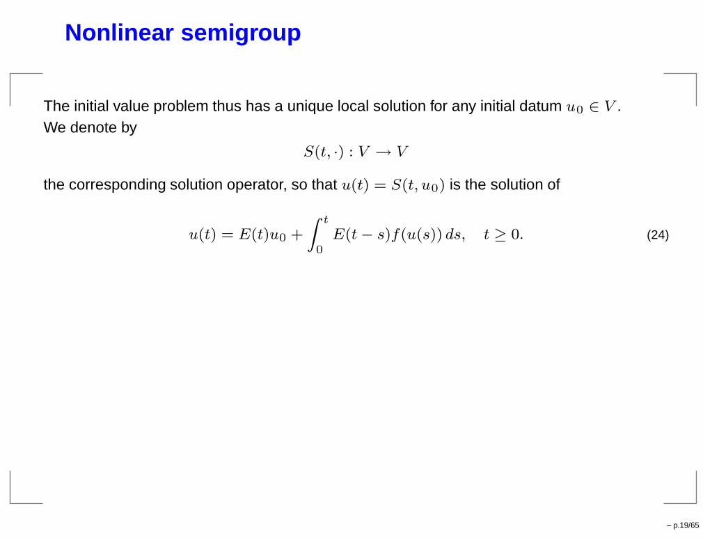
Nonlinear semigroup

The initial value problem thus has a unique local solution for any initial datum u0 ∈ V .We denote by

S(t, ·) : V → V

the corresponding solution operator, so that u(t) = S(t, u0) is the solution of

u(t) = E(t)u0 +

Z t

0E(t− s)f(u(s)) ds, t ≥ 0. (24)

– p.19/65

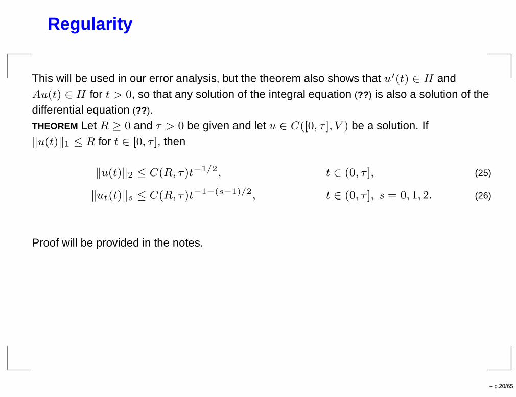
Regularity

This will be used in our error analysis, but the theorem also shows that u′(t) ∈ H andAu(t) ∈ H for t > 0, so that any solution of the integral equation (??) is also a solution of thedifferential equation (??).THEOREM Let R ≥ 0 and τ > 0 be given and let u ∈ C([0, τ ], V ) be a solution. If‖u(t)‖1 ≤ R for t ∈ [0, τ ], then

‖u(t)‖2 ≤ C(R, τ)t−1/2, t ∈ (0, τ ], (25)

‖ut(t)‖s ≤ C(R, τ)t−1−(s−1)/2, t ∈ (0, τ ], s = 0, 1, 2. (26)

Proof will be provided in the notes.

– p.20/65

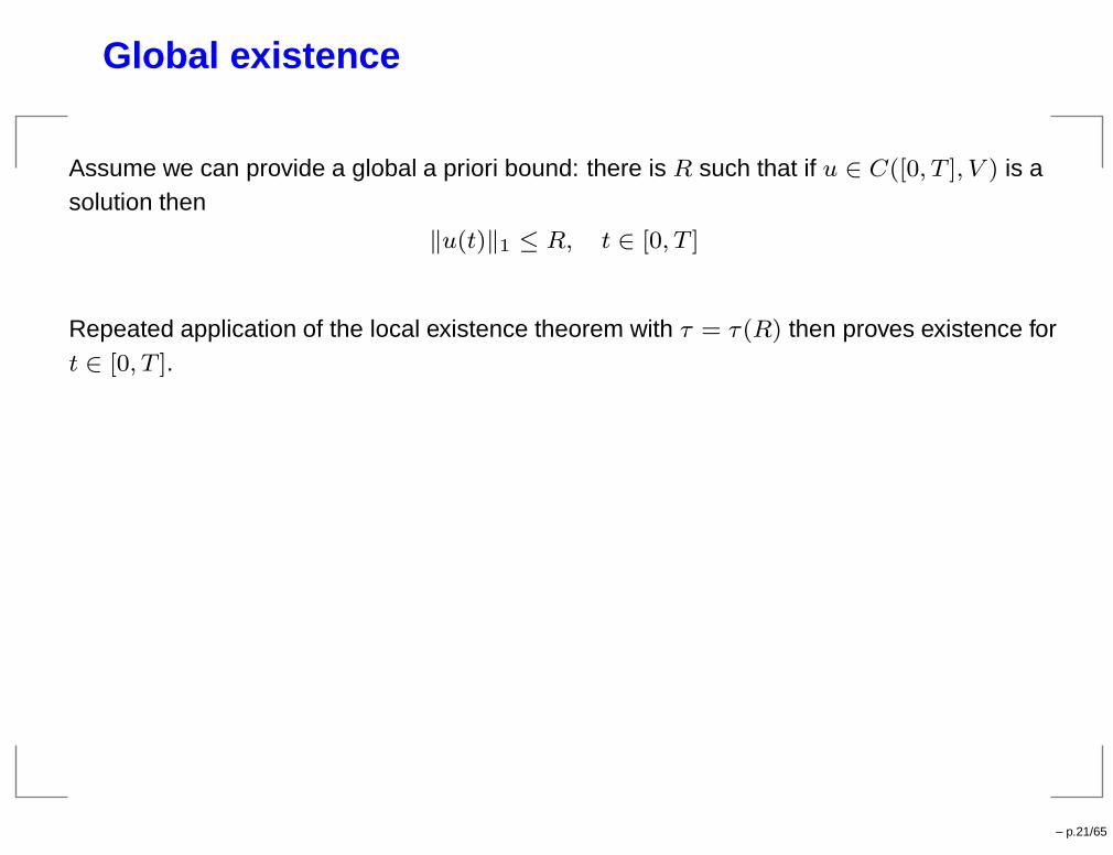
Global existence

Assume we can provide a global a priori bound: there is R such that if u ∈ C([0, T ], V ) is asolution then

‖u(t)‖1 ≤ R, t ∈ [0, T ]

Repeated application of the local existence theorem with τ = τ(R) then proves existence fort ∈ [0, T ].

– p.21/65

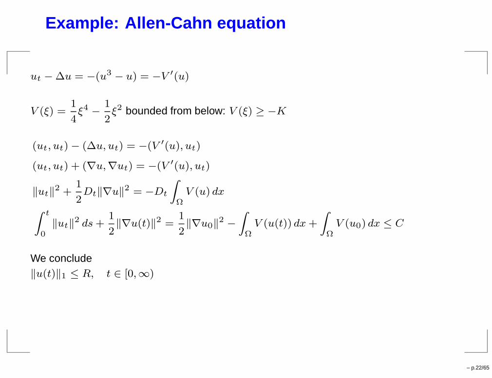
Example: Allen-Cahn equation

ut − ∆u = −(u3 − u) = −V ′(u)

V (ξ) =1

4ξ4 −

1

2ξ2 bounded from below: V (ξ) ≥ −K

(ut, ut) − (∆u, ut) = −(V ′(u), ut)

(ut, ut) + (∇u,∇ut) = −(V ′(u), ut)

‖ut‖2 +

1

2Dt‖∇u‖

2 = −Dt

Z

ΩV (u) dx

Z t

0‖ut‖

2 ds+1

2‖∇u(t)‖2 =

1

2‖∇u0‖

2 −

Z

ΩV (u(t)) dx+

Z

ΩV (u0) dx ≤ C

We conclude‖u(t)‖1 ≤ R, t ∈ [0,∞)

– p.22/65

Lecture 2: Finite element method

– p.23/65

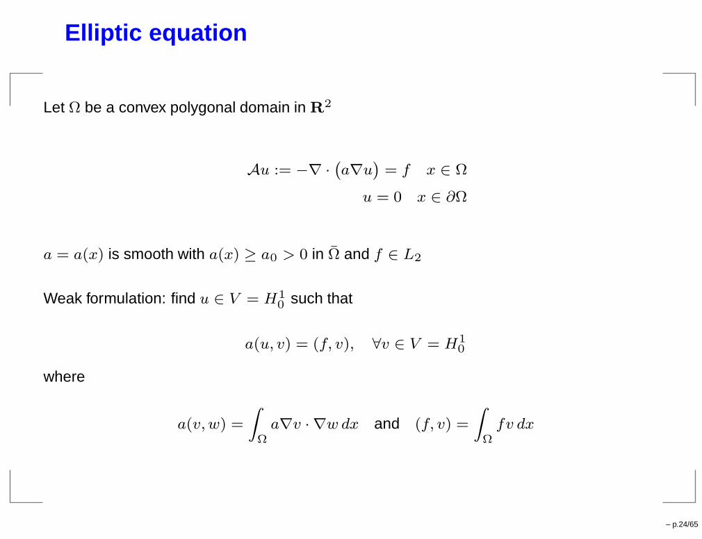
Elliptic equation

Let Ω be a convex polygonal domain in R2

Au := −∇ ·`

a∇u´

= f x ∈ Ω

u = 0 x ∈ ∂Ω

a = a(x) is smooth with a(x) ≥ a0 > 0 in Ω and f ∈ L2

Weak formulation: find u ∈ V = H10 such that

a(u, v) = (f, v), ∀v ∈ V = H10

where

a(v,w) =

Z

Ωa∇v · ∇w dx and (f, v) =

Z

Ωfv dx

– p.24/65

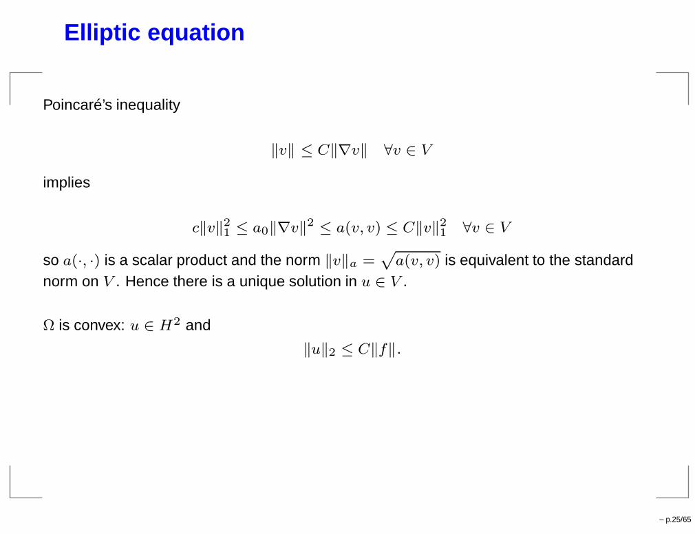
Elliptic equation

Poincaré’s inequality

‖v‖ ≤ C‖∇v‖ ∀v ∈ V

implies

c‖v‖21 ≤ a0‖∇v‖

2 ≤ a(v, v) ≤ C‖v‖21 ∀v ∈ V

so a(·, ·) is a scalar product and the norm ‖v‖a =p

a(v, v) is equivalent to the standardnorm on V . Hence there is a unique solution in u ∈ V .

Ω is convex: u ∈ H2 and

‖u‖2 ≤ C‖f‖.

– p.25/65

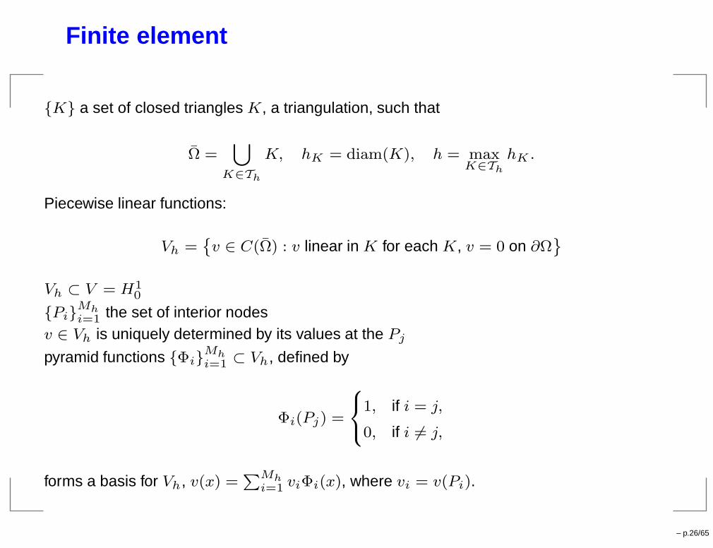
Finite element

K a set of closed triangles K, a triangulation, such that

Ω =[

K∈Th

K, hK = diam(K), h = maxK∈Th

hK .

Piecewise linear functions:

Vh =˘

v ∈ C(Ω) : v linear in K for each K, v = 0 on ∂Ω¯

Vh ⊂ V = H10

PiMhi=1 the set of interior nodes

v ∈ Vh is uniquely determined by its values at the Pj

pyramid functions ΦiMhi=1 ⊂ Vh, defined by

Φi(Pj) =

8

<

:

1, if i = j,

0, if i 6= j,

forms a basis for Vh, v(x) =PMh

i=1 viΦi(x), where vi = v(Pi).

– p.26/65

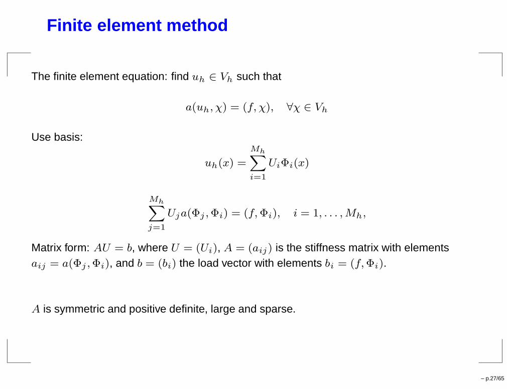
Finite element method

The finite element equation: find uh ∈ Vh such that

a(uh, χ) = (f, χ), ∀χ ∈ Vh

Use basis:

uh(x) =

MhX

i=1

UiΦi(x)

MhX

j=1

Uja(Φj ,Φi) = (f,Φi), i = 1, . . . ,Mh,

Matrix form: AU = b, where U = (Ui), A = (aij) is the stiffness matrix with elementsaij = a(Φj ,Φi), and b = (bi) the load vector with elements bi = (f,Φi).

A is symmetric and positive definite, large and sparse.

– p.27/65

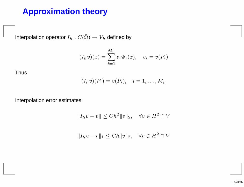
Approximation theory

Interpolation operator Ih : C(Ω) → Vh defined by

(Ihv)(x) =

MhX

i=1

viΦi(x), vi = v(Pi)

Thus

(Ihv)(Pi) = v(Pi), i = 1, . . . ,Mh

Interpolation error estimates:

‖Ihv − v‖ ≤ Ch2‖v‖2, ∀v ∈ H2 ∩ V

‖Ihv − v‖1 ≤ Ch‖v‖2, ∀v ∈ H2 ∩ V

– p.28/65

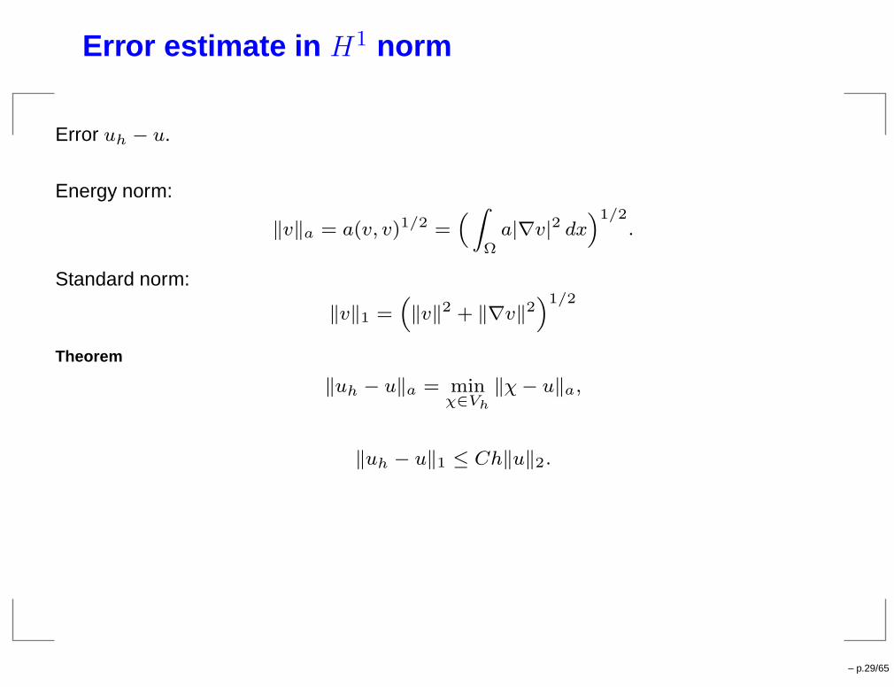
Error estimate in H1 norm

Error uh − u.

Energy norm:

‖v‖a = a(v, v)1/2 =“

Z

Ωa|∇v|2 dx

”1/2.

Standard norm:

‖v‖1 =“

‖v‖2 + ‖∇v‖2”1/2

Theorem

‖uh − u‖a = minχ∈Vh

‖χ− u‖a,

‖uh − u‖1 ≤ Ch‖u‖2.

– p.29/65

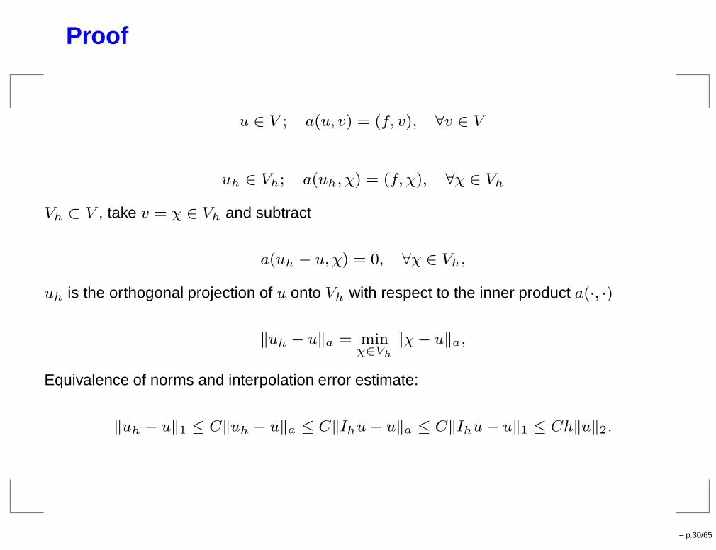
Proof

u ∈ V ; a(u, v) = (f, v), ∀v ∈ V

uh ∈ Vh; a(uh, χ) = (f, χ), ∀χ ∈ Vh

Vh ⊂ V , take v = χ ∈ Vh and subtract

a(uh − u, χ) = 0, ∀χ ∈ Vh,

uh is the orthogonal projection of u onto Vh with respect to the inner product a(·, ·)

‖uh − u‖a = minχ∈Vh

‖χ− u‖a,

Equivalence of norms and interpolation error estimate:

‖uh − u‖1 ≤ C‖uh − u‖a ≤ C‖Ihu− u‖a ≤ C‖Ihu− u‖1 ≤ Ch‖u‖2.

– p.30/65

Error estimate in L2 norm

Theorem

‖uh − u‖ ≤ Ch2‖u‖2.

– p.31/65

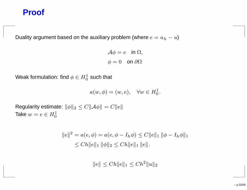
Proof

Duality argument based on the auxiliary problem (where e = uh − u)

Aφ = e in Ω,

φ = 0 on ∂Ω

Weak formulation: find φ ∈ H10 such that

a(w,φ) = (w, e), ∀w ∈ H10 .

Regularity estimate: ‖φ‖2 ≤ C‖Aφ‖ = C‖e‖

Take w = e ∈ H10

‖e‖2 = a(e, φ) = a(e, φ− Ihφ) ≤ C‖e‖1 ‖φ− Ihφ‖1

≤ Ch‖e‖1 ‖φ‖2 ≤ Ch‖e‖1 ‖e‖.

‖e‖ ≤ Ch‖e‖1 ≤ Ch2‖u‖2

– p.32/65

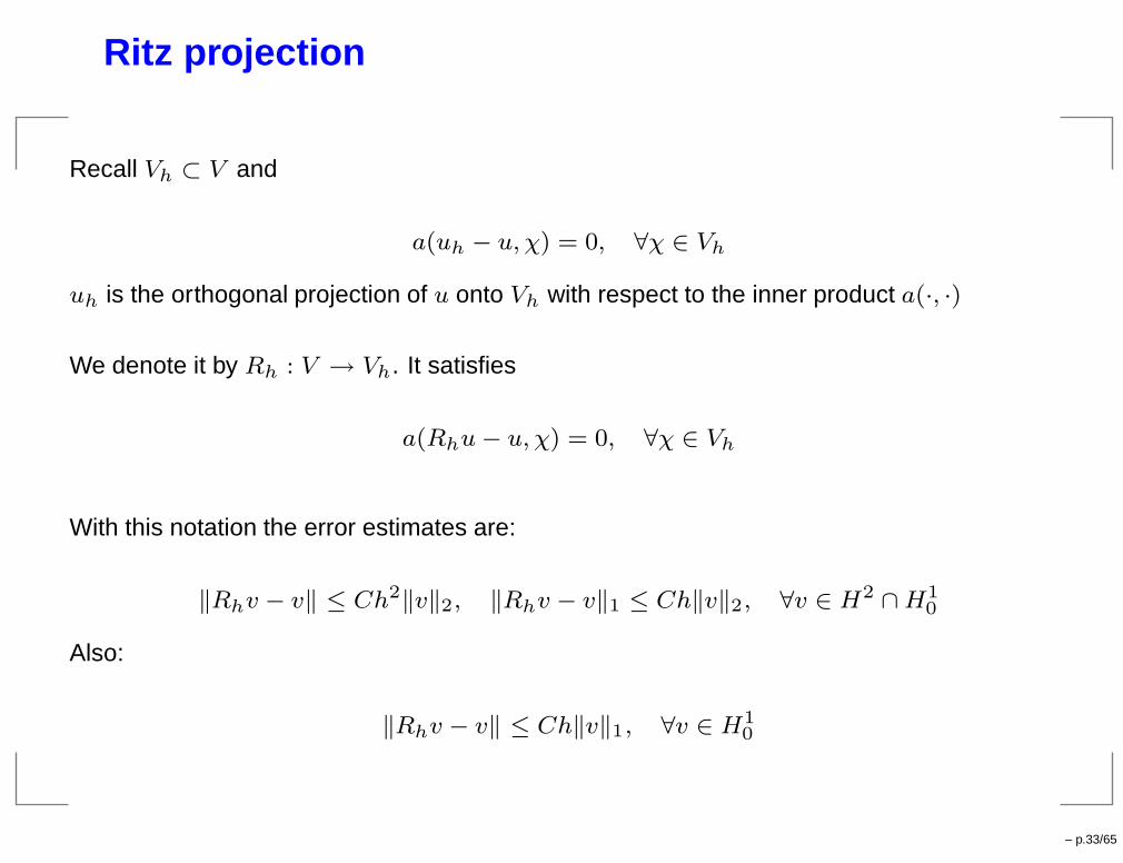
Ritz projection

Recall Vh ⊂ V and

a(uh − u, χ) = 0, ∀χ ∈ Vh

uh is the orthogonal projection of u onto Vh with respect to the inner product a(·, ·)

We denote it by Rh : V → Vh. It satisfies

a(Rhu− u, χ) = 0, ∀χ ∈ Vh

With this notation the error estimates are:

‖Rhv − v‖ ≤ Ch2‖v‖2, ‖Rhv − v‖1 ≤ Ch‖v‖2, ∀v ∈ H2 ∩H10

Also:

‖Rhv − v‖ ≤ Ch‖v‖1, ∀v ∈ H10

– p.33/65

Lecture 3: Finite elements for semilinear parabolic PDE

– p.34/65

Abstract framework

Find u(t) ∈ V such that

u′ +Au = f(u), t > 0; u(0) = u0.

Linear homogenous equation:

u′ +Au = 0, t > 0; u(0) = u0; u(t) = E(t)u0

By Duhamel’s principle:

u(t) = E(t)u0 +

Z t

0E(t− s)f(u(s)) ds, t ≥ 0.

– p.35/65

Local existence and regularity

THEOREM For any R0 > 0 there is τ = τ(R0) such that there is a unique solutionu ∈ C([0, τ ], V ) for any initial value u0 ∈ V with ‖u0‖1 ≤ R0. Moreover, there is c such that‖u‖L∞([0,τ ],V ) ≤ cR0.

THEOREM Let R ≥ 0 and τ > 0 be given and let u ∈ C([0, τ ], V ) be a solution. If‖u(t)‖1 ≤ R for t ∈ [0, τ ], then

‖u(t)‖2 ≤ C(R, τ)t−1/2, t ∈ (0, τ ],

‖ut(t)‖s ≤ C(R, τ)t−1−(s−1)/2, t ∈ (0, τ ], s = 0, 1, 2.

Global solution on [0, T ] if we can prove a priori bound

‖u(t)‖1 ≤ R, t ∈ [0, T ]

– p.36/65

Finite element method

Linear elliptic equation:−∇ ·

`

a∇u´

= f x ∈ Ω

u = 0 x ∈ ∂Ω

Weak formulation: find u ∈ V = H10 such that

a(u, v) = (f, v), ∀v ∈ V = H10

where

a(v,w) =

Z

Ωa∇v · ∇w dx and (f, v) =

Z

Ωfv dx

The finite element equation: find uh ∈ Vh such that

a(uh, χ) = (f, χ), ∀χ ∈ Vh

– p.37/65

Error estimates

‖uh − u‖1 ≤ Ch‖u‖2

‖uh − u‖ ≤ Ch2‖u‖2

– p.38/65

Ritz projection

Recall Vh ⊂ V and

a(uh − u, χ) = 0, ∀χ ∈ Vh

uh is the orthogonal projection of u onto Vh with respect to the inner product a(·, ·)

We denote it by Rh : V → Vh. It satisfies

a(Rhu− u, χ) = 0, ∀χ ∈ Vh

With this notation the error estimates are:

‖Rhv − v‖ ≤ Ch2‖v‖2, ‖Rhv − v‖1 ≤ Ch‖v‖2, ∀v ∈ H2 ∩H10

Also:

‖Rhv − v‖ ≤ Ch‖v‖1, ∀v ∈ H10

– p.39/65

Spatially semidiscrete approximation

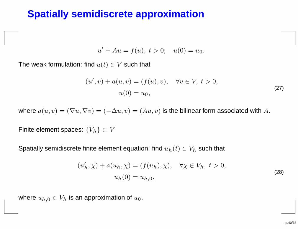
u′ +Au = f(u), t > 0; u(0) = u0.

The weak formulation: find u(t) ∈ V such that

(u′, v) + a(u, v) = (f(u), v), ∀v ∈ V, t > 0,

u(0) = u0,(27)

where a(u, v) = (∇u,∇v) = (−∆u, v) = (Au, v) is the bilinear form associated with A.

Finite element spaces: Vh ⊂ V

Spatially semidiscrete finite element equation: find uh(t) ∈ Vh such that

(u′h, χ) + a(uh, χ) = (f(uh), χ), ∀χ ∈ Vh, t > 0,

uh(0) = uh,0,(28)

where uh,0 ∈ Vh is an approximation of u0.

– p.40/65

Abstract framework

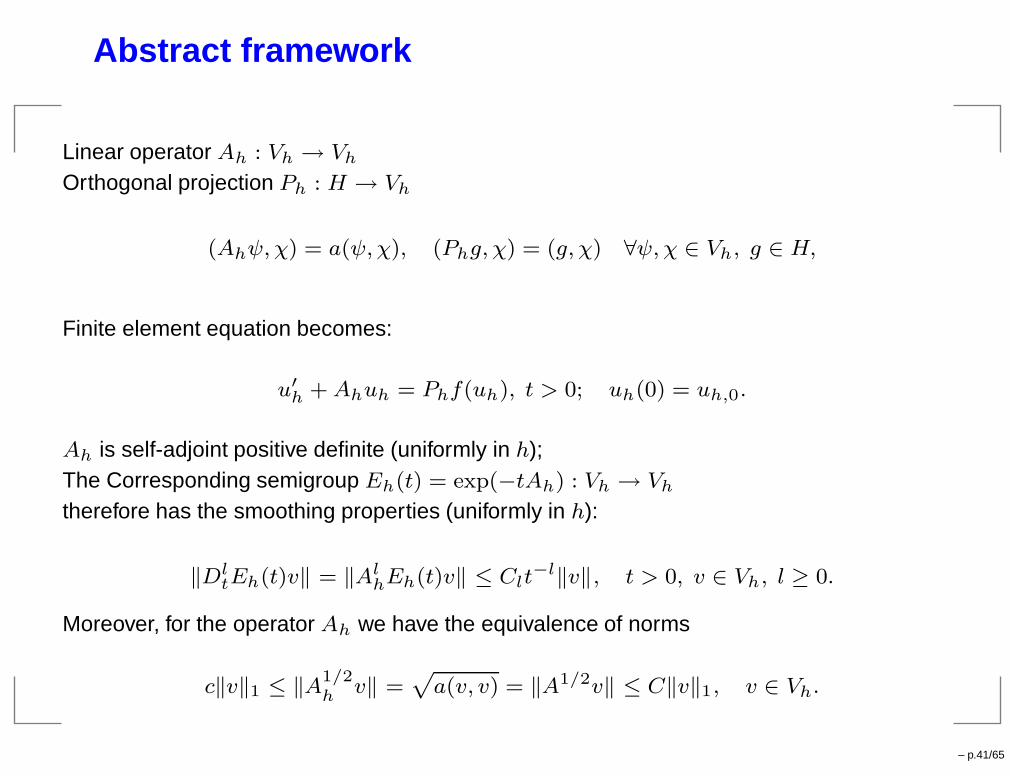
Linear operator Ah : Vh → Vh

Orthogonal projection Ph : H → Vh

(Ahψ, χ) = a(ψ,χ), (Phg, χ) = (g, χ) ∀ψ, χ ∈ Vh, g ∈ H,

Finite element equation becomes:

u′h +Ahuh = Phf(uh), t > 0; uh(0) = uh,0.

Ah is self-adjoint positive definite (uniformly in h);The Corresponding semigroup Eh(t) = exp(−tAh) : Vh → Vh

therefore has the smoothing properties (uniformly in h):

‖DltEh(t)v‖ = ‖Al

hEh(t)v‖ ≤ Clt−l‖v‖, t > 0, v ∈ Vh, l ≥ 0.

Moreover, for the operator Ah we have the equivalence of norms

c‖v‖1 ≤ ‖A1/2h v‖ =

p

a(v, v) = ‖A1/2v‖ ≤ C‖v‖1, v ∈ Vh.

– p.41/65

Abstract formulation

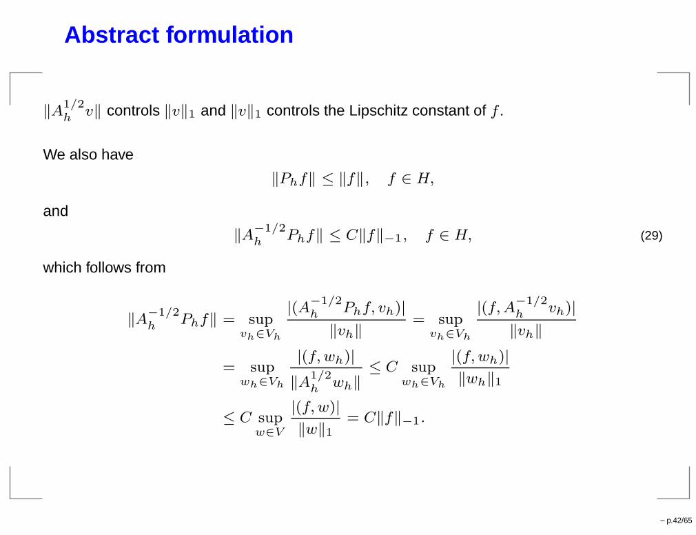
‖A1/2h v‖ controls ‖v‖1 and ‖v‖1 controls the Lipschitz constant of f .

We also have

‖Phf‖ ≤ ‖f‖, f ∈ H,

and

‖A−1/2h Phf‖ ≤ C‖f‖−1, f ∈ H, (29)

which follows from

‖A−1/2h Phf‖ = sup

vh∈Vh

|(A−1/2h Phf, vh)|

‖vh‖= sup

vh∈Vh

|(f,A−1/2h vh)|

‖vh‖

= supwh∈Vh

|(f,wh)|

‖A1/2h wh‖

≤ C supwh∈Vh

|(f,wh)|

‖wh‖1

≤ C supw∈V

|(f,w)|

‖w‖1= C‖f‖−1.

– p.42/65

Abstract formulation

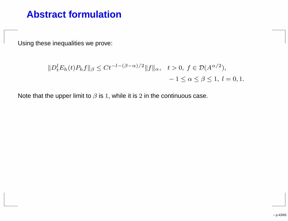
Using these inequalities we prove:

‖DltEh(t)Phf‖β ≤ Ct−l−(β−α)/2‖f‖α, t > 0, f ∈ D(Aα/2),

− 1 ≤ α ≤ β ≤ 1, l = 0, 1.

Note that the upper limit to β is 1, while it is 2 in the continuous case.

– p.43/65

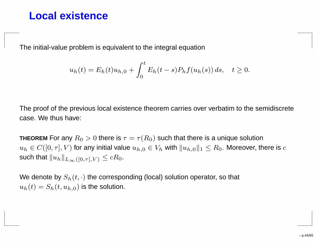
Local existence

The initial-value problem is equivalent to the integral equation

uh(t) = Eh(t)uh,0 +

Z t

0Eh(t− s)Phf(uh(s)) ds, t ≥ 0.

The proof of the previous local existence theorem carries over verbatim to the semidiscretecase. We thus have:

THEOREM For any R0 > 0 there is τ = τ(R0) such that there is a unique solutionuh ∈ C([0, τ ], V ) for any initial value uh,0 ∈ Vh with ‖uh,0‖1 ≤ R0. Moreover, there is csuch that ‖uh‖L∞([0,τ ],V ) ≤ cR0.

We denote by Sh(t, ·) the corresponding (local) solution operator, so thatuh(t) = Sh(t, uh,0) is the solution.

– p.44/65

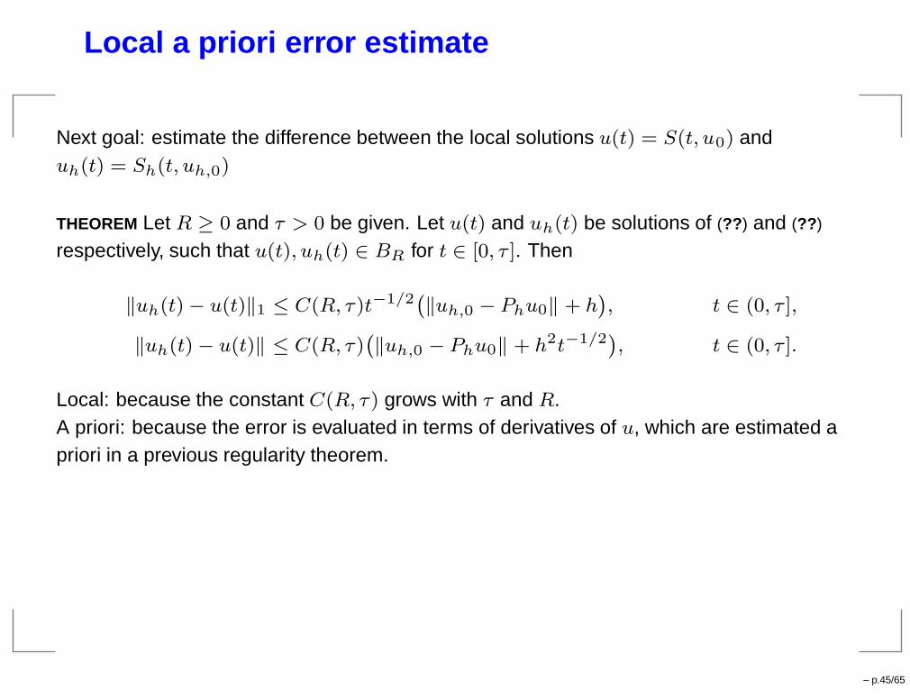
Local a priori error estimate

Next goal: estimate the difference between the local solutions u(t) = S(t, u0) anduh(t) = Sh(t, uh,0)

THEOREM Let R ≥ 0 and τ > 0 be given. Let u(t) and uh(t) be solutions of (??) and (??)

respectively, such that u(t), uh(t) ∈ BR for t ∈ [0, τ ]. Then

‖uh(t) − u(t)‖1 ≤ C(R, τ)t−1/2`

‖uh,0 − Phu0‖ + h´

, t ∈ (0, τ ],

‖uh(t) − u(t)‖ ≤ C(R, τ)`

‖uh,0 − Phu0‖ + h2t−1/2´

, t ∈ (0, τ ].

Local: because the constant C(R, τ) grows with τ and R.A priori: because the error is evaluated in terms of derivatives of u, which are estimated apriori in a previous regularity theorem.

– p.45/65

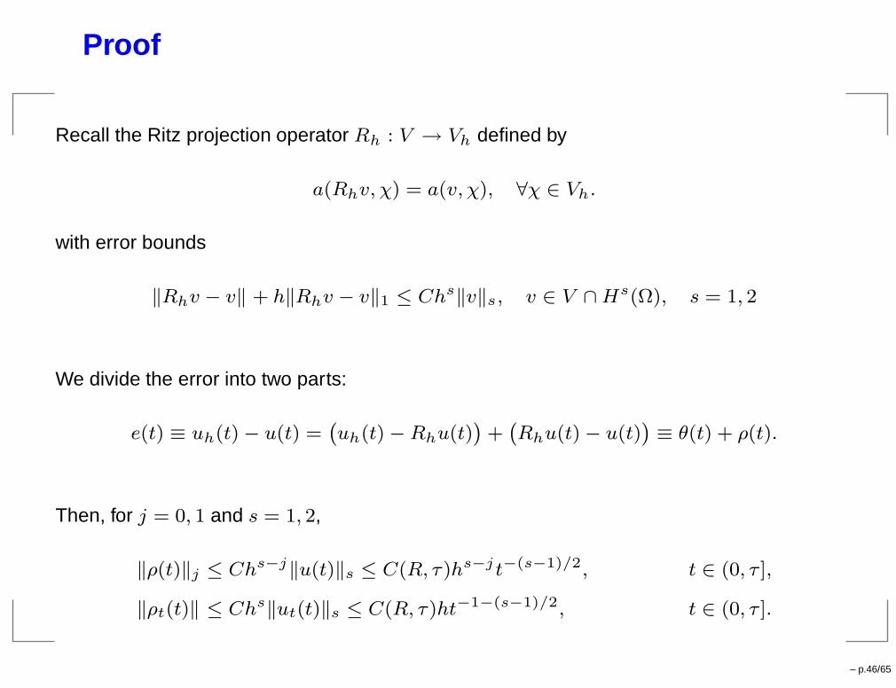
Proof

Recall the Ritz projection operator Rh : V → Vh defined by

a(Rhv, χ) = a(v, χ), ∀χ ∈ Vh.

with error bounds

‖Rhv − v‖ + h‖Rhv − v‖1 ≤ Chs‖v‖s, v ∈ V ∩Hs(Ω), s = 1, 2

We divide the error into two parts:

e(t) ≡ uh(t) − u(t) =`

uh(t) −Rhu(t)´

+`

Rhu(t) − u(t)´

≡ θ(t) + ρ(t).

Then, for j = 0, 1 and s = 1, 2,

‖ρ(t)‖j ≤ Chs−j‖u(t)‖s ≤ C(R, τ)hs−jt−(s−1)/2, t ∈ (0, τ ],

‖ρt(t)‖ ≤ Chs‖ut(t)‖s ≤ C(R, τ)ht−1−(s−1)/2, t ∈ (0, τ ].

– p.46/65

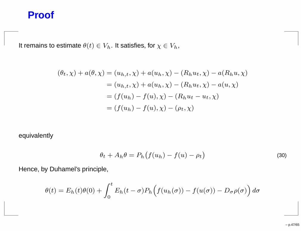
Proof

It remains to estimate θ(t) ∈ Vh. It satisfies, for χ ∈ Vh,

(θt, χ) + a(θ, χ) = (uh,t, χ) + a(uh, χ) − (Rhut, χ) − a(Rhu,χ)

= (uh,t, χ) + a(uh, χ) − (Rhut, χ) − a(u, χ)

= (f(uh) − f(u), χ) − (Rhut − ut, χ)

= (f(uh) − f(u), χ) − (ρt, χ)

equivalently

θt +Ahθ = Ph

`

f(uh) − f(u) − ρt´

(30)

Hence, by Duhamel’s principle,

θ(t) = Eh(t)θ(0) +

Z t

0Eh(t− σ)Ph

“

f(uh(σ)) − f(u(σ)) −Dσρ(σ)”

dσ

– p.47/65

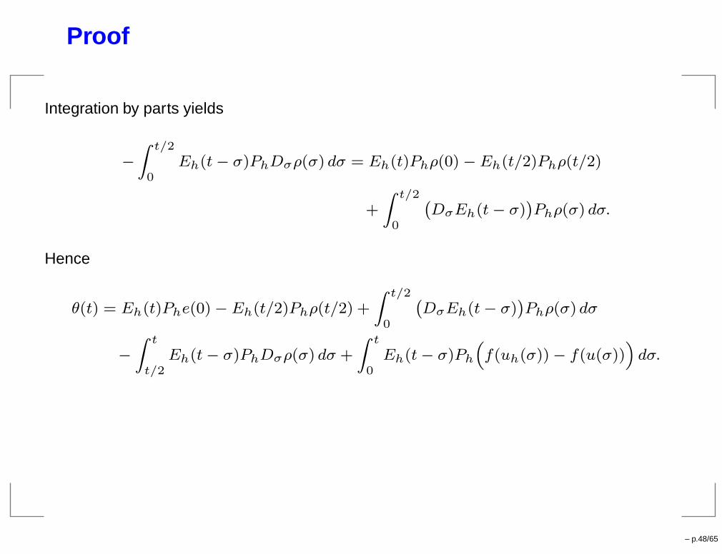
Proof

Integration by parts yields

−

Z t/2

0Eh(t− σ)PhDσρ(σ) dσ = Eh(t)Phρ(0) −Eh(t/2)Phρ(t/2)

+

Z t/2

0

`

DσEh(t− σ)´

Phρ(σ) dσ.

Hence

θ(t) = Eh(t)Phe(0) − Eh(t/2)Phρ(t/2) +

Z t/2

0

`

DσEh(t− σ)´

Phρ(σ) dσ

−

Z t

t/2Eh(t− σ)PhDσρ(σ) dσ +

Z t

0Eh(t− σ)Ph

“

f(uh(σ)) − f(u(σ))”

dσ.

– p.48/65

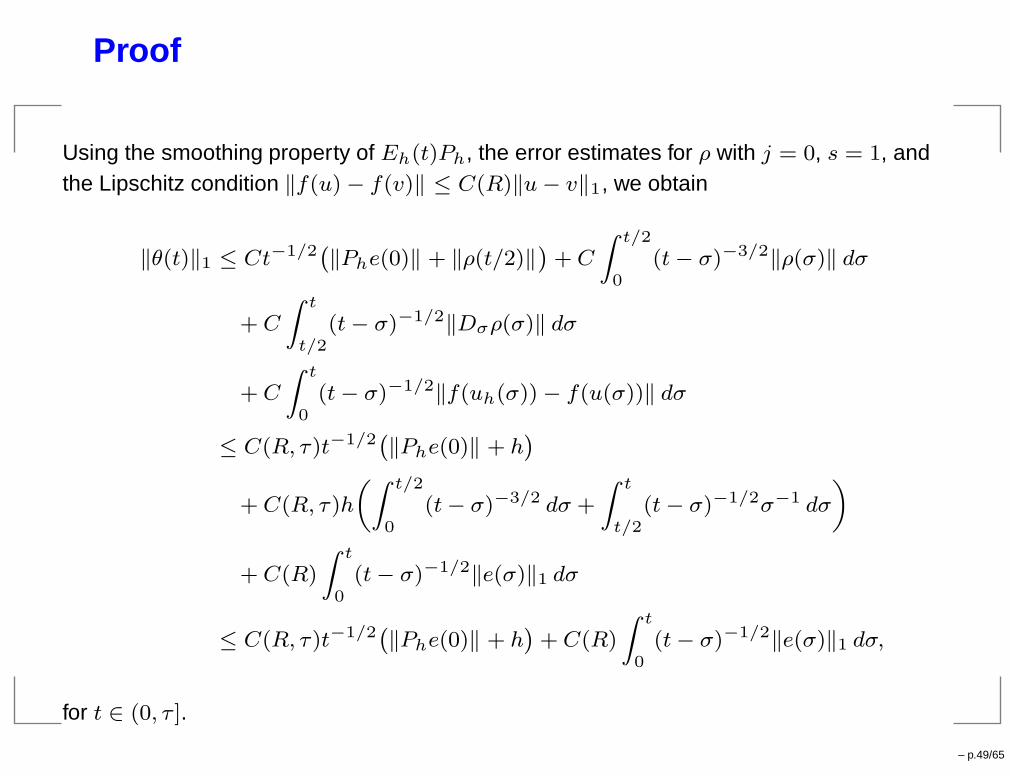
Proof

Using the smoothing property of Eh(t)Ph, the error estimates for ρ with j = 0, s = 1, andthe Lipschitz condition ‖f(u) − f(v)‖ ≤ C(R)‖u− v‖1, we obtain

‖θ(t)‖1 ≤ Ct−1/2`

‖Phe(0)‖ + ‖ρ(t/2)‖´

+ C

Z t/2

0(t− σ)−3/2‖ρ(σ)‖ dσ

+ C

Z t

t/2(t− σ)−1/2‖Dσρ(σ)‖ dσ

+ C

Z t

0(t− σ)−1/2‖f(uh(σ)) − f(u(σ))‖ dσ

≤ C(R, τ)t−1/2`

‖Phe(0)‖ + h´

+ C(R, τ)h

„Z t/2

0(t− σ)−3/2 dσ +

Z t

t/2(t− σ)−1/2σ−1 dσ

«

+ C(R)

Z t

0(t− σ)−1/2‖e(σ)‖1 dσ

≤ C(R, τ)t−1/2`

‖Phe(0)‖ + h´

+ C(R)

Z t

0(t− σ)−1/2‖e(σ)‖1 dσ,

for t ∈ (0, τ ].

– p.49/65

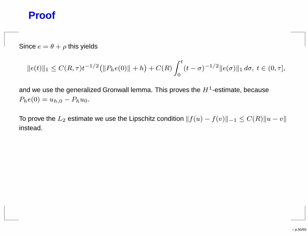
Proof

Since e = θ + ρ this yields

‖e(t)‖1 ≤ C(R, τ)t−1/2`

‖Phe(0)‖ + h´

+ C(R)

Z t

0(t− σ)−1/2‖e(σ)‖1 dσ, t ∈ (0, τ ],

and we use the generalized Gronwall lemma. This proves the H1-estimate, becausePhe(0) = uh,0 − Phu0.

To prove the L2 estimate we use the Lipschitz condition ‖f(u) − f(v)‖−1 ≤ C(R)‖u− v‖

instead.

– p.50/65

Generalized Gronwall lemma

Lemma Let the function ϕ(t, τ) ≥ 0 be continuous for 0 ≤ τ < t ≤ T . If

ϕ(t, τ) ≤ A (t− τ)−1+α + B

Z t

τ(t− s)−1+βϕ(s, τ) ds, 0 ≤ τ < t ≤ T,

for some constants A,B ≥ 0, α, β > 0, then there is a constant C = C(B,T, α, β) such that

ϕ(t, τ) ≤ CA (t− τ)−1+α, 0 ≤ τ < t ≤ T.

The constant in Gronwall’s lemma grows exponentially with the length T of the time interval.Hence, results derived by means of this lemma are often useful only for short time intervals.

– p.51/65

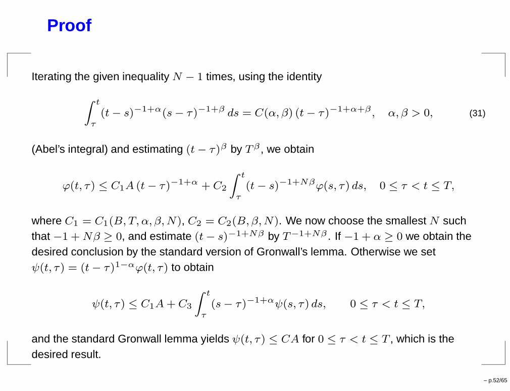
Proof

Iterating the given inequality N − 1 times, using the identity

Z t

τ(t− s)−1+α(s− τ)−1+β ds = C(α, β) (t− τ)−1+α+β , α, β > 0, (31)

(Abel’s integral) and estimating (t− τ)β by Tβ , we obtain

ϕ(t, τ) ≤ C1A (t− τ)−1+α + C2

Z t

τ(t− s)−1+Nβϕ(s, τ) ds, 0 ≤ τ < t ≤ T,

where C1 = C1(B,T, α, β,N), C2 = C2(B, β,N). We now choose the smallest N suchthat −1 +Nβ ≥ 0, and estimate (t− s)−1+Nβ by T−1+Nβ . If −1 + α ≥ 0 we obtain thedesired conclusion by the standard version of Gronwall’s lemma. Otherwise we setψ(t, τ) = (t− τ)1−αϕ(t, τ) to obtain

ψ(t, τ) ≤ C1A+ C3

Z t

τ(s− τ)−1+αψ(s, τ) ds, 0 ≤ τ < t ≤ T,

and the standard Gronwall lemma yields ψ(t, τ) ≤ CA for 0 ≤ τ < t ≤ T , which is thedesired result.

– p.52/65

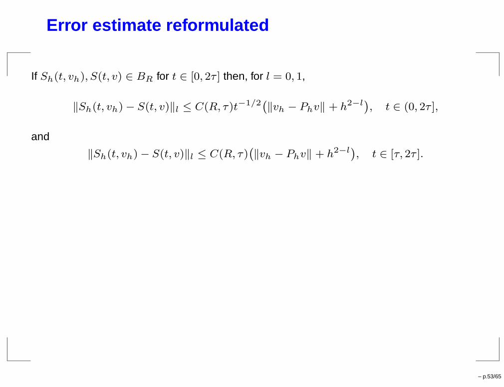
Error estimate reformulated

If Sh(t, vh), S(t, v) ∈ BR for t ∈ [0, 2τ ] then, for l = 0, 1,

‖Sh(t, vh) − S(t, v)‖l ≤ C(R, τ)t−1/2`

‖vh − Phv‖ + h2−l´

, t ∈ (0, 2τ ],

and

‖Sh(t, vh) − S(t, v)‖l ≤ C(R, τ)`

‖vh − Phv‖ + h2−l´

, t ∈ [τ, 2τ ].

– p.53/65

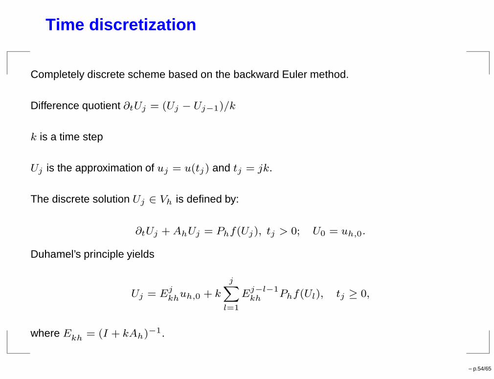
Time discretization

Completely discrete scheme based on the backward Euler method.

Difference quotient ∂tUj = (Uj − Uj−1)/k

k is a time step

Uj is the approximation of uj = u(tj) and tj = jk.

The discrete solution Uj ∈ Vh is defined by:

∂tUj +AhUj = Phf(Uj), tj > 0; U0 = uh,0.

Duhamel’s principle yields

Uj = Ejkhuh,0 + k

jX

l=1

Ej−l−1kh Phf(Ul), tj ≥ 0,

where Ekh = (I + kAh)−1.

– p.54/65

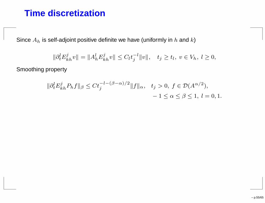
Time discretization

Since Ah is self-adjoint positive definite we have (uniformly in h and k)

‖∂ltE

jkhv‖ = ‖Al

hEjkhv‖ ≤ Clt

−lj ‖v‖, tj ≥ tl, v ∈ Vh, l ≥ 0,

Smoothing property

‖∂ltE

jkhPhf‖β ≤ Ct

−l−(β−α)/2j ‖f‖α, tj > 0, f ∈ D(Aα/2),

− 1 ≤ α ≤ β ≤ 1, l = 0, 1.

– p.55/65

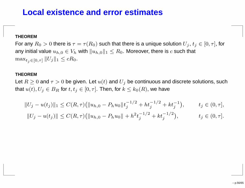
Local existence and error estimates

THEOREM

For any R0 > 0 there is τ = τ(R0) such that there is a unique solution Uj , tj ∈ [0, τ ], forany initial value uh,0 ∈ Vh with ‖uh,0‖1 ≤ R0. Moreover, there is c such thatmaxtj∈[0,τ ] ‖Uj‖1 ≤ cR0.

THEOREM

Let R ≥ 0 and τ > 0 be given. Let u(t) and Uj be continuous and discrete solutions, suchthat u(t), Uj ∈ BR for t, tj ∈ [0, τ ]. Then, for k ≤ k0(R), we have

‖Uj − u(tj)‖1 ≤ C(R, τ)`

‖uh,0 − Phu0‖t−1/2j + ht

−1/2j + kt−1

j

´

, tj ∈ (0, τ ],

‖Uj − u(tj)‖ ≤ C(R, τ)`

‖uh,0 − Phu0‖ + h2t−1/2j + kt

−1/2j

´

, tj ∈ (0, τ ].

– p.56/65

Lecture 4: Application to dynamical systems theory

– p.57/65

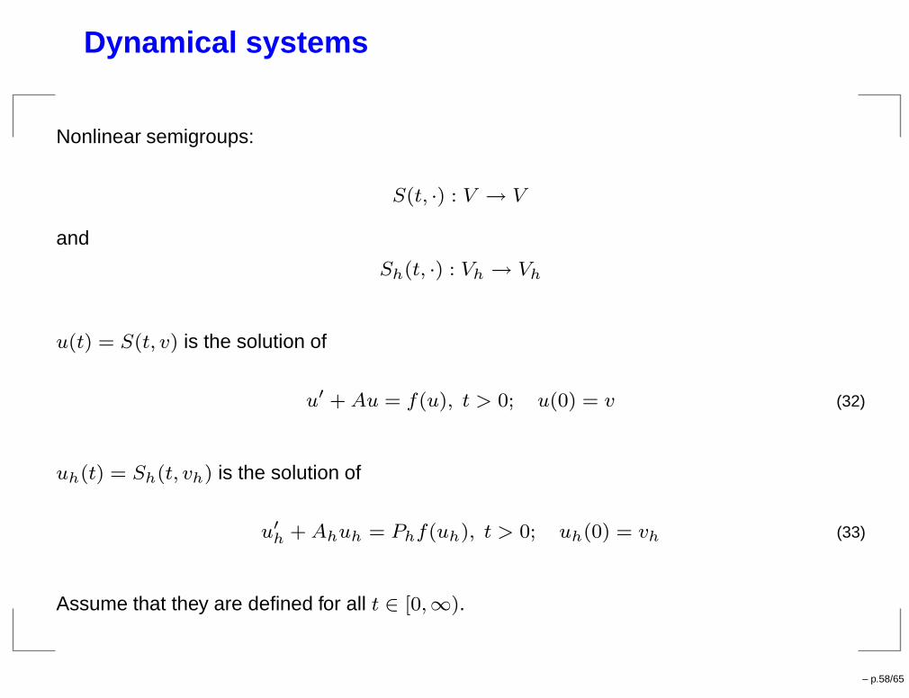
Dynamical systems

Nonlinear semigroups:

S(t, ·) : V → V

and

Sh(t, ·) : Vh → Vh

u(t) = S(t, v) is the solution of

u′ + Au = f(u), t > 0; u(0) = v (32)

uh(t) = Sh(t, vh) is the solution of

u′h + Ahuh = Phf(uh), t > 0; uh(0) = vh (33)

Assume that they are defined for all t ∈ [0,∞).

– p.58/65

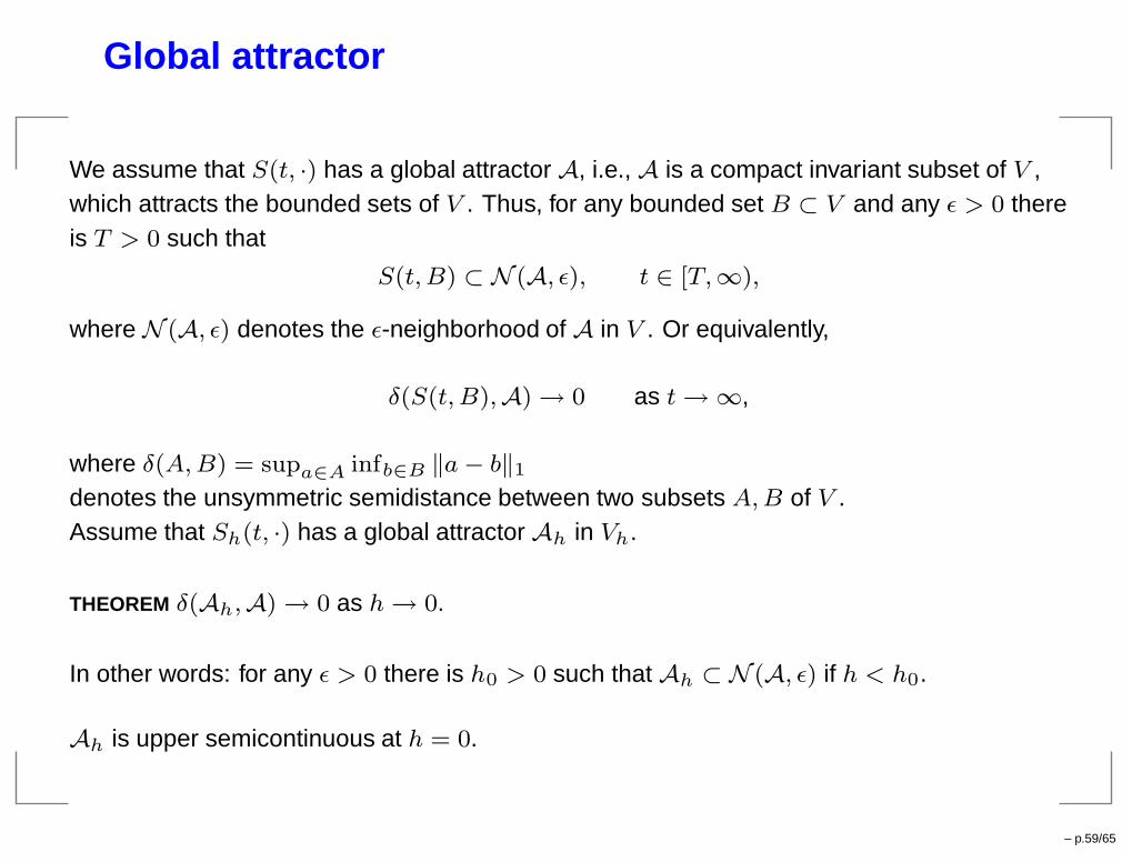
Global attractor

We assume that S(t, ·) has a global attractor A, i.e., A is a compact invariant subset of V ,which attracts the bounded sets of V . Thus, for any bounded set B ⊂ V and any ε > 0 thereis T > 0 such that

S(t,B) ⊂ N (A, ε), t ∈ [T,∞),

where N (A, ε) denotes the ε-neighborhood of A in V . Or equivalently,

δ(S(t, B),A) → 0 as t→ ∞,

where δ(A,B) = supa∈A infb∈B ‖a− b‖1

denotes the unsymmetric semidistance between two subsets A,B of V .Assume that Sh(t, ·) has a global attractor Ah in Vh.

THEOREM δ(Ah,A) → 0 as h→ 0.

In other words: for any ε > 0 there is h0 > 0 such that Ah ⊂ N (A, ε) if h < h0.

Ah is upper semicontinuous at h = 0.

– p.59/65

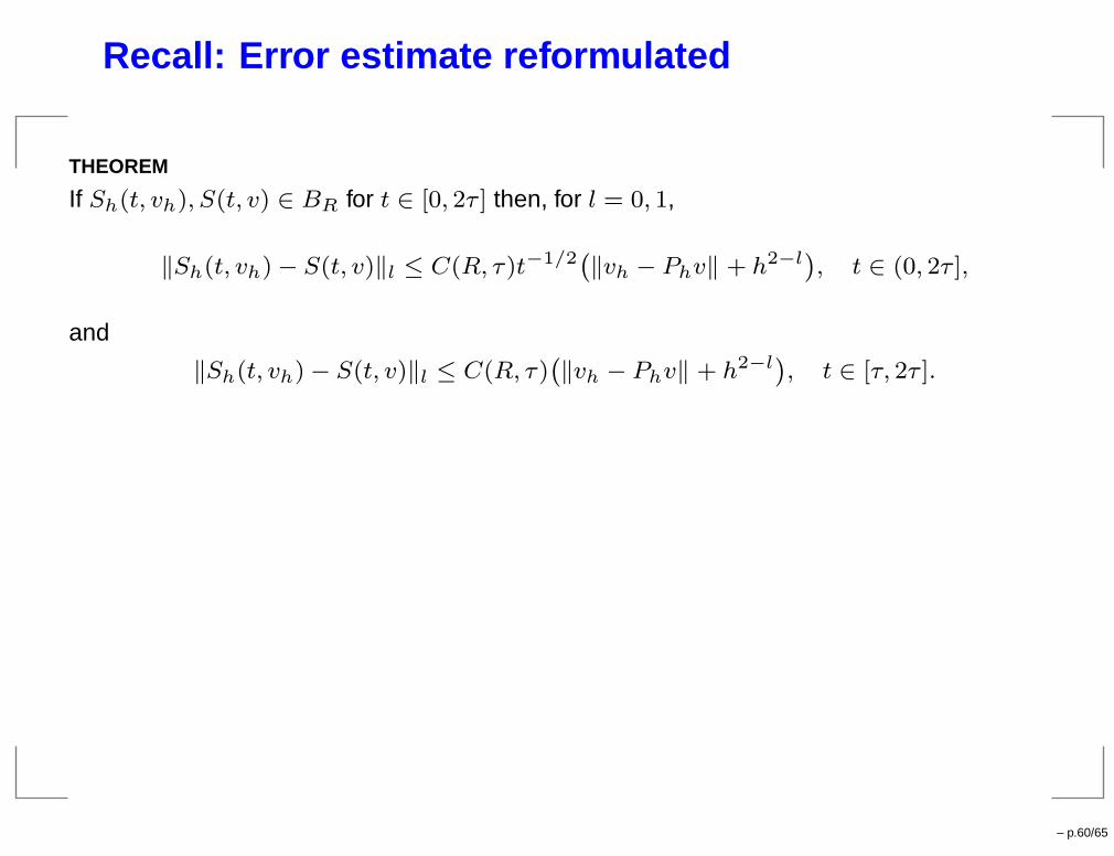
Recall: Error estimate reformulated

THEOREM

If Sh(t, vh), S(t, v) ∈ BR for t ∈ [0, 2τ ] then, for l = 0, 1,

‖Sh(t, vh) − S(t, v)‖l ≤ C(R, τ)t−1/2`

‖vh − Phv‖ + h2−l´

, t ∈ (0, 2τ ],

and

‖Sh(t, vh) − S(t, v)‖l ≤ C(R, τ)`

‖vh − Phv‖ + h2−l´

, t ∈ [τ, 2τ ].

– p.60/65

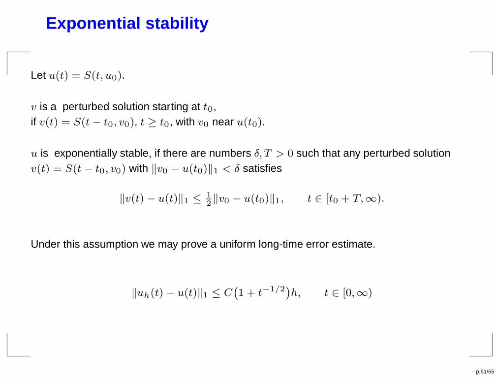
Exponential stability

Let u(t) = S(t, u0).

v is a perturbed solution starting at t0,if v(t) = S(t− t0, v0), t ≥ t0, with v0 near u(t0).

u is exponentially stable, if there are numbers δ, T > 0 such that any perturbed solutionv(t) = S(t− t0, v0) with ‖v0 − u(t0)‖1 < δ satisfies

‖v(t) − u(t)‖1 ≤ 12‖v0 − u(t0)‖1, t ∈ [t0 + T,∞).

Under this assumption we may prove a uniform long-time error estimate.

‖uh(t) − u(t)‖1 ≤ C`

1 + t−1/2´

h, t ∈ [0,∞)

– p.61/65

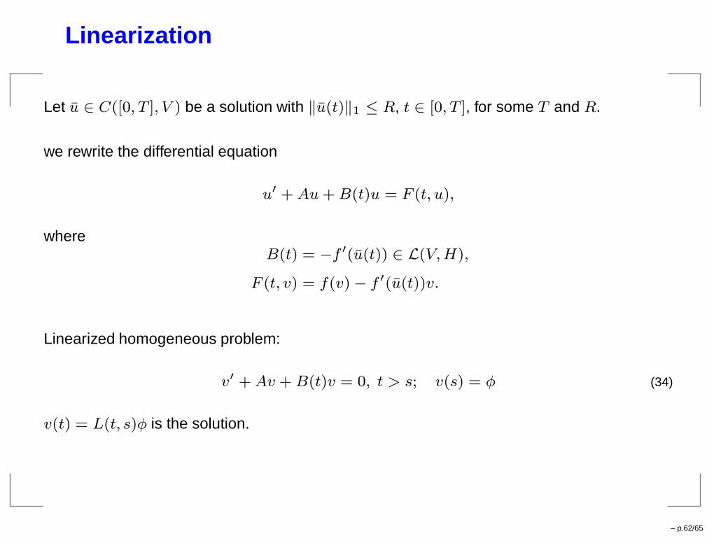
Linearization

Let u ∈ C([0, T ], V ) be a solution with ‖u(t)‖1 ≤ R, t ∈ [0, T ], for some T and R.

we rewrite the differential equation

u′ +Au+B(t)u = F (t, u),

whereB(t) = −f ′(u(t)) ∈ L(V,H),

F (t, v) = f(v) − f ′(u(t))v.

Linearized homogeneous problem:

v′ +Av + B(t)v = 0, t > s; v(s) = φ (34)

v(t) = L(t, s)φ is the solution.

– p.62/65

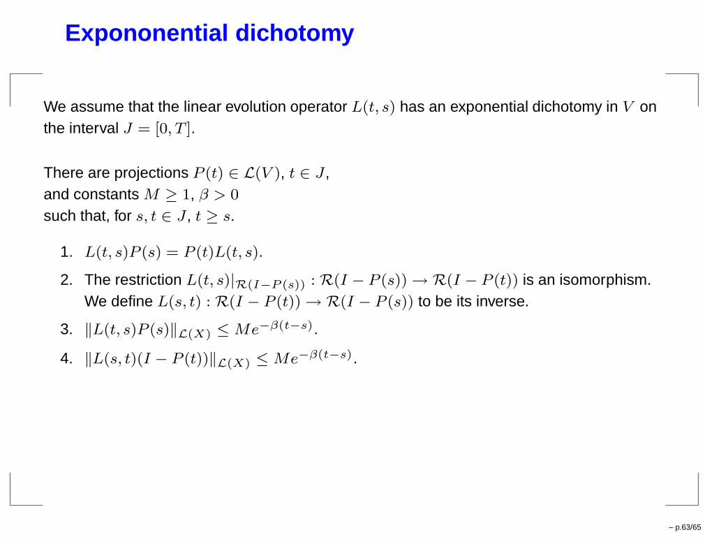
Expononential dichotomy

We assume that the linear evolution operator L(t, s) has an exponential dichotomy in V onthe interval J = [0, T ].

There are projections P (t) ∈ L(V ), t ∈ J ,and constants M ≥ 1, β > 0

such that, for s, t ∈ J , t ≥ s.

1. L(t, s)P (s) = P (t)L(t, s).

2. The restriction L(t, s)|R(I−P (s)) : R(I − P (s)) → R(I − P (t)) is an isomorphism.We define L(s, t) : R(I − P (t)) → R(I − P (s)) to be its inverse.

3. ‖L(t, s)P (s)‖L(X) ≤Me−β(t−s).

4. ‖L(s, t)(I − P (t))‖L(X) ≤Me−β(t−s).

– p.63/65

Shadowing

THEOREM

Let u ∈ C([0, T ], V ) be a solution of with

maxt∈[0,T ]

‖u(t)‖1 ≤ R,

for some T and R.Assume that the solution operator L(t, s) of the linearized problem has an exponentialdichotomy in V on the interval [0, T ]. Then there are numbers ρ0 and C such that, for eachsolution uh(t) = Sh(t, uh,0), t ∈ [0, T ], with

maxt∈[0,T ]

‖uh(t) − u(t)‖1 ≤ ρ0,

there is a solution u such that

‖uh(t) − u(t)‖1 ≤ C`

1 + t−1/2´

h, t ∈ (0, T ].

The numerical solution uh is shadowed by an exact solution u in a neighborhood of u.

– p.64/65

Open problem

Numerical shadowing: prove that shadowing can be detected “a posteriori” in the numericalcomputation.

– p.65/65