Classification Of Partial Differential

Equations And Their Solution

Characteristics

8th Indo-German Winter Academy 2009, IIT Roorkee, India, December 13-19, 2009

High Performance Computing for Engineering Problems

Characteristics

Swetha Jain Kothari

IIT Roorkee

Tutors:

Prof. S. Mishra

Prof. U. Rüde

Prof. V. Buwa

Contents

• Partial Differential Equations

• Linear Partial Differential Equations

• Classification of second order linear PDEs

• Canonical Forms

• Characteristics• Characteristics

• Initial and Boundary Conditions

• Elliptic Partial Differential Equations

• Parabolic Partial Differential Equations

• Hyperbolic Partial Differential Equations

• Summary

Partial Differential Equations

• An equation which involves several independentvariables (usually denoted x, y, z, t, …..), a dependentfunction u of these variables, and the partialderivatives of the dependent function u with respect tothe independent variables such as

F(x, y, z, t, ….., u , u , u , u , ….., u , u , ….., u , …..)=0F(x, y, z, t, ….., ux, uy, uz, ut, ….., uxx, uyy, ….., uxy, …..)=0

is called a partial differential equation.

• Partial differential equations are used to formulate,and thus aid the solution of, problems involvingfunctions of several variables; such as the propagationof sound or heat, electrostatics, electrodynamics, fluidflow, and elasticity.

Partial Differential Equations cont.

• Examples:

i. ut=k(uxx + uyy + uzz) [linear three-dimensionalheat equation]

ii. uxx + uyy + uzz=0 [Laplace equation in threeii. uxx + uyy + uzz=0 [Laplace equation in threedimensions]

iii. utt=c2(uxx + uyy + uzz) [linear three-dimensionalwave equation]

iv. ut + uux=µuxx [nonlinear one-dimensionalBurger equation]

Partial Differential Equations cont.

• The order of a partial differential equation is

the order of the highest derivative occurring in

the equation.

• All the above examples are second order• All the above examples are second order

partial differential equations.

• ut=uuxxx + sin x is an example for third order

partial differential equation.

Ordinary Differential Equations vs.

Partial Differential Equations

Partial Differential Equations

• A relatively simple partial

differential equation is

ux(x, y)=0

Ordinary Differential Equations

• The analogous ordinary

differential equation is

u’(x)=0

• General solution of the

above equation is

u(x, y)=f(y)

• General solution involves

arbitrary functions

• General solution of the

above equation is

u(x)=c

• General solution involves

arbitrary constants

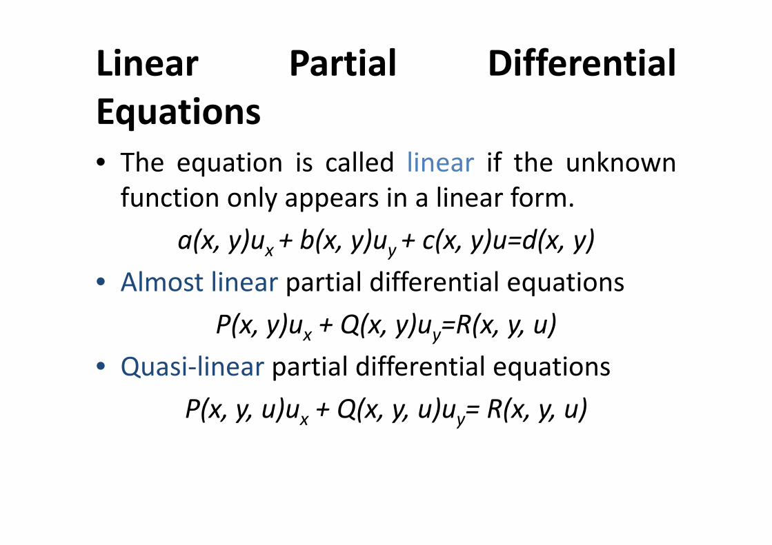
Linear Partial Differential

Equations

• The equation is called linear if the unknown

function only appears in a linear form.

a(x, y)ux + b(x, y)uy + c(x, y)u=d(x, y)

• Almost linear partial differential equations• Almost linear partial differential equations

P(x, y)ux + Q(x, y)uy=R(x, y, u)

• Quasi-linear partial differential equations

P(x, y, u)ux + Q(x, y, u)uy= R(x, y, u)

Classification of second order linear

PDEs

Consider the second order linear PDE in two variablesAuxx + Buxy +Cuyy +Dux+ Euy+ Fu=G (1)

The discriminant

d=B2(x0, y0) – 4A(x0, y0)C(x0, y0)

At (x0, y0), the equation is said to beAt (x0, y0), the equation is said to be

� Elliptic if d<0

� Parabolic if d=0

� Hyperbolic if d>0

If this is true at all points in a domain Ω, then theequation is said to be elliptic, parabolic, or hyperbolicin that domain

Classification of second order linear

PDEs cont.

• If there are n independent variables x1, x2 , ...,

xn, a general linear partial differential equation

of second order has the form

• ∑∑a u plus lower order terms =0• ∑∑ai,juxixjplus lower order terms =0

• The classification depends upon the signature

of the eigenvalues of the coefficient matrix.

Classification of second order linear

PDEs cont.

i. Elliptic: The eigenvalues are all positive or all

negative.

ii. Parabolic : The eigenvalues are all positive or

all negative, save one which is zero.all negative, save one which is zero.

iii. Hyperbolic: There is only one negative

eigenvalue and all the rest are positive, or

there is only one positive eigenvalue and all

the rest are negative.

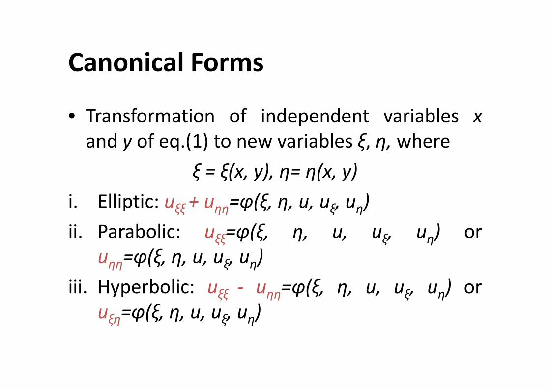
Canonical Forms

• Transformation of independent variables x

and y of eq.(1) to new variables ξ, η, where

ξ = ξ(x, y), η= η(x, y)

i. Elliptic: u + u =φ(ξ, η, u, u , u )i. Elliptic: uξξ + uηη=φ(ξ, η, u, uξ, uη)

ii. Parabolic: uξξ=φ(ξ, η, u, uξ, uη) or

uηη=φ(ξ, η, u, uξ, uη)

iii. Hyperbolic: uξξ - uηη=φ(ξ, η, u, uξ, uη) or

uξη=φ(ξ, η, u, uξ, uη)

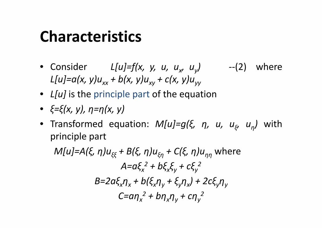
Characteristics

• Consider L[u]=f(x, y, u, ux, uy) --(2) where

L[u]=a(x, y)uxx + b(x, y)uxy + c(x, y)uyy

• L[u] is the principle part of the equation

• ξ=ξ(x, y), η=η(x, y)• ξ=ξ(x, y), η=η(x, y)

• Transformed equation: M[u]=g(ξ, η, u, uξ, uη) with

principle part

M[u]=A(ξ, η)uξξ + B(ξ, η)uξη + C(ξ, η)uηη where

A=aξx2 + bξxξy + cξy

2

B=2aξxηx + b(ξxηy + ξyηx) + 2cξyηy

C=aηx2 + bηxηy + cηy

2

Characteristics cont.

• An integral of an ordinary differential equation is a

function φ whose level curves, φ(x, y)=k, characterize

solutions of the equation implicitly.

• a(x, y)ξx2 + b(x, y)ξxξy + c(x, y)ξy

2=0 iff ξ is an integral of

the ordinary differential equationthe ordinary differential equation

a(x, y)y’2 - b(x, y)y’ + c(x, y)=0 --(3)

=>y’=[b(x, y) ± {b2(x, y) – 4a(x, y)c(x, y)}1/2]/2a

• An integral curve, φ(x, y)=k, of (3) is a characteristic

curve, and (3) is called the characteristic equation for

the partial differential equation (2)

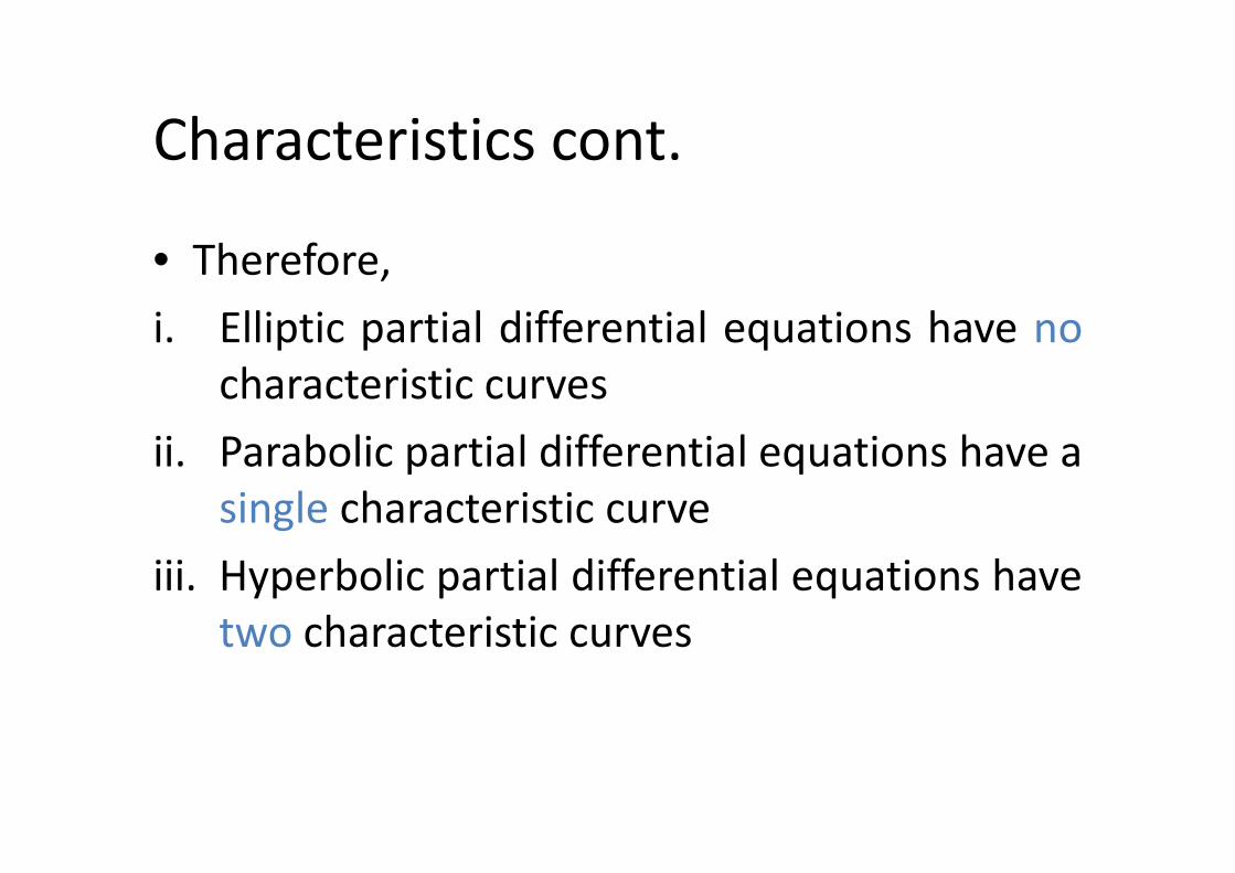
Characteristics cont.

• Therefore,

i. Elliptic partial differential equations have no

characteristic curves

ii. Parabolic partial differential equations have aii. Parabolic partial differential equations have a

single characteristic curve

iii. Hyperbolic partial differential equations have

two characteristic curves

Initial and Boundary Conditions

(a) Elliptic Equations: Boundary conditions

e.g. uxx + uyy=G in a finite region R bounded by a

closed curve C.

yy

C

x

R

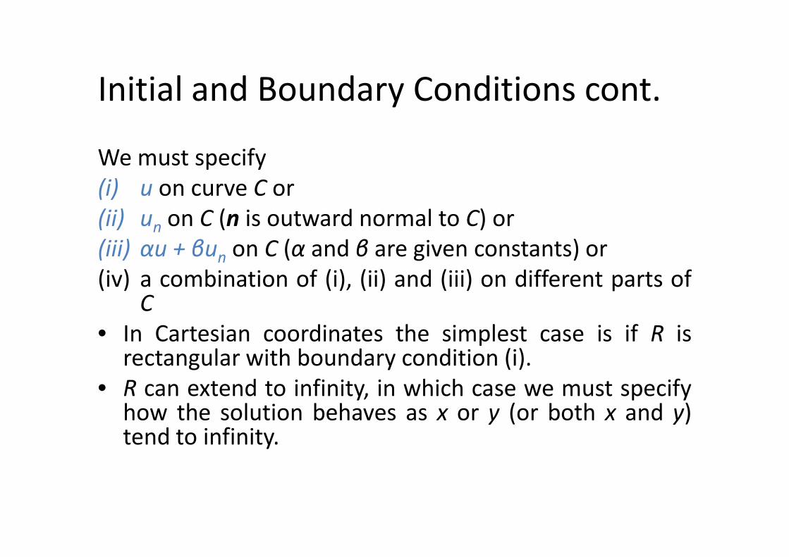
Initial and Boundary Conditions cont.

We must specify

(i) u on curve C or

(ii) un on C (n is outward normal to C) or

(iii) αu + βun on C (α and β are given constants) or

(iv) a combination of (i), (ii) and (iii) on different parts of(iv) a combination of (i), (ii) and (iii) on different parts ofC

• In Cartesian coordinates the simplest case is if R isrectangular with boundary condition (i).

• R can extend to infinity, in which case we must specifyhow the solution behaves as x or y (or both x and y)tend to infinity.

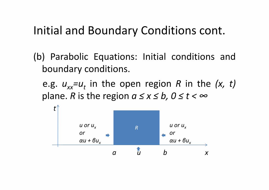
Initial and Boundary Conditions cont.

(b) Parabolic Equations: Initial conditions and

boundary conditions.

e.g. uxx=ut in the open region R in the (x, t)

plane. R is the region a ≤ x ≤ b, 0 ≤ t < ∞

R

plane. R is the region a ≤ x ≤ b, 0 ≤ t < ∞

t

a u b x

u or ux

or

αu + βux

u or ux

or

αu + βux

Initial and Boundary Conditions cont.

• We must specify u on t=0 (i.e. u(x, 0)) for a ≤ x ≤

b. This is an initial condition (e.g. an initial

temperature distribution) and suitable boundary

conditions x on a and b are as shown.conditions x on a and b are as shown.

(c) Hyperbolic Equations: e.g. uxx=utt Initial

conditions and boundary conditions as for (b)

except that we must also specify ut at t=0 for a ≤ x

≤ b (in addition to u) and R is the region a ≤ x ≤ b,

-∞ < t < ∞

Elliptic Partial Differential Equations

• The discriminant B2 - 4AC < 0

• Solutions of elliptic PDEs are as smooth as the

coefficients allow, within the interior of the

region where the equation and solutions areregion where the equation and solutions are

defined.

• For example, solutions of Laplace's equation

are analytic within the domain where they are

defined, but solutions may assume boundary

values that are not smooth.

Elliptic Partial Differential Equations

cont.

• Region of Influence: Entire domain

• Region of Dependence: Entire domain

• Any disturbance at P is felt throughout the

domain

P

Elliptic Partial Differential Equations cont.

Examples:

(i) Laplace Equation: ∆u=0

• The Laplace equation is often encountered in heat andmass transfer theory, fluid mechanics, elasticity,electrostatics, and other areas of mechanics andelectrostatics, and other areas of mechanics andphysics.

• The two dimensional Laplace equation has thefollowing form:

uxx + uyy=0 in the Cartesian coordinate system,

(1/r)(rur)r +(1/r2)uθθ=0 in the polar coordinate system

Laplace Equation cont.

• A function which satisfies Laplace's equation issaid to be harmonic.

• A solution to Laplace's equation has the propertythat the average value over a spherical surface isequal to the value at the center of the sphereequal to the value at the center of the sphere(Gauss’ harmonic function theorem).

• Solutions have no local maxima or minima.

• Because Laplace's equation is linear andhomogeneous, the superposition of any twosolutions is also a solution

Laplace Equation cont.

Solution of Laplace’s equation:

Consider uxx + uyy=0 (2)

Solve by separation of variables

Let u=X(x)Y(y)Let u=X(x)Y(y)

Substituting it in (2), we get

(1/X)X’’=-(1/Y)Y’’=k

Solution of Laplace Equation cont.

i. k=p2: X=c1epx + c2e-px, Y=c3cos py + c4sin py

ii. k=-p2: X=c5cos px + c6sin px, Y=c7epy + c8e-py

iii. k=0: X=c9x + c10, Y=c11y + c12

Thus, various possible solutions are:Thus, various possible solutions are:

u=(c1epx + c2e-px)(c3cos py + c4sin py)

u=(c5cos px + c6sin px)(c7epy + c8e-py)

u=(c9x + c10)(c11y + c12)

Laplace Equation cont.

Analytic functions:

• The real and imaginary parts of a complex analyticfunction both satisfy the Laplace equation.

• If f(x + iy)=u(x, y) + iv(x, y) is an analytic function, thenu + u =0, v + v =0uxx + uyy=0, vxx + vyy=0

• The close connection between the Laplace equationand analytic functions implies that any solution of theLaplace equation has derivatives of all orders, and canbe expanded in a power series, at least inside a circlethat does not enclose a singularity.

Elliptic Partial Differential Equations

cont.

(ii) Poisson Equation: ∆u + Φ=0

• The two dimensional Poisson equation has thefollowing form:

uxx + uyy + f(x, y)=0 in the Cartesian coordinate system,

(1/r)(ru ) +(1/r2)u + g(r, θ)=0 in the polar coordinate (1/r)(rur)r +(1/r2)uθθ + g(r, θ)=0 in the polar coordinate system

• Poisson’s equation is a partial differential equationwith broad utility in electrostatics, mechanicalengineering and theoretical physics.

• E.g. In electrostatics: ∆V=-ρ/ε

Elliptic Partial Differential Equations

cont.

(iii) Helmholtz Equation: ∆u + λu=-Φ

• Many problems related to steady state

oscillations (mechanical, acoustical, thermal,

electromagnetic) lead to the two dimensionalelectromagnetic) lead to the two dimensional

Helmholtz equation. For ¸ λ< 0, this equation

describes mass transfer processes with

volume chemical reactions of the first order.

Helmholtz Equation cont.

• The two dimensional Helmholtz equation has

the following form:

uxx + uyy + λu=-f(x, y) in the Cartesian coordinate

system,system,

(1/r)(rur)r +(1/r2)uθθ + λu=-g(r, θ) in the polar

coordinate system

Parabolic Partial Differential

Equations

• The discriminant B2 - 4AC = 0

• Equations that are parabolic at every point can

be transformed into a form analogous to the

heat equation by a change of independentheat equation by a change of independent

variables.

• Solutions smooth out as the transformed time

variable increases

Parabolic Partial Differential Equations

cont.

• Region of influence: Part of domain away from

initial data line from the characteristic curve

• Region of dependence: Part of domain from

the initial data line to the characteristic curvethe initial data line to the characteristic curve

PRegionofinfluence

Regionofdependence

Boundary

Boundary

Characteristic curve at P

Parabolic Partial Differential Equations

cont.

Examples:

i. ut=auxx heat equation (linear heat equation)

ii. ut=auxx + f(x, t) non-homogeneous heat

equationequation

iii. ut=auxx + bux + cu + f(x, t) convective heat

equation with a source

iv. ut=a(urr + (1/r)ur) heat equation with axial

symmetry

Parabolic Partial Differential Equations

cont.

v. ut=a(urr + (1/r)ur) + g(r, t) heat equation with

axial symmetry (with a source)

vi. ut=a(urr + (2/r)ur) heat equation with central

symmetrysymmetry

vii. ut=a(urr + (2/r)ur) + g(r, t) heat equation with

central symmetry (with a source)

viii.iħut=-(ħ2/2m)uxx + h(x)u Schrodinger

equation (linear schrodinger equation)

Parabolic Partial Differential Equations

cont.

• Heat equation: ut=a∆u

• The maximum value of u is either earlier in time than

the region of concern or on the edge of the region of

concern.

• even if u has a discontinuity at an initial time t = t , the• even if u has a discontinuity at an initial time t = t0, the

temperature becomes smooth as soon as t > t0. For

example, if a bar of metal has temperature 0 and

another has temperature 100 and they are stuck

together end to end, then very quickly the temperature

at the point of connection is 50 and the graph of the

temperature is smoothly running from 0 to 100.

Parabolic Partial Differential Equations

cont.

Solution of the heat equation:

Consider ut=auxx (3)

• In plain English, this equation says that the temperature at a given time and point will rise or fall at a rate proportional to the difference between the temperature at that point and the average temperature a rate proportional to the difference between the temperature at that point and the average temperature near that point.

Solve by separation of variables

Let u(x, t)=X(x)T(t)

Substituting this in (3), we get

X’’/X=T’/aT=k

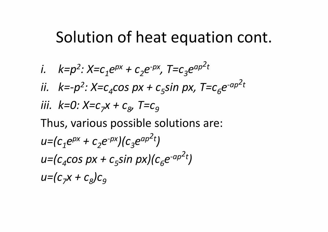
Solution of heat equation cont.

i. k=p2: X=c1epx + c2e-px, T=c3eap2t

ii. k=-p2: X=c4cos px + c5sin px, T=c6e-ap2t

iii. k=0: X=c7x + c8, T=c9

Thus, various possible solutions are:Thus, various possible solutions are:

u=(c1epx + c2e-px)(c3eap2t)

u=(c4cos px + c5sin px)(c6e-ap2t)

u=(c7x + c8)c9

Parabolic Partial Differential Equations

cont.

• Let u(x, t) be a continuous function and a

solution of ut=auxx for 0 ≤ x ≤ l, 0 ≤ t ≤ T, where

T > 0 is a fixed time. Then the maximum and

minimum values of u are attained either at minimum values of u are attained either at

time t=0 or at the end points x=0 and x=l at

some time in the interval 0 ≤ t ≤ T

Hyperbolic Partial Differential

Equations

• The discriminant B2 - 4AC > 0

• Hyperbolic equations retain any discontinuities of

functions or derivatives in the initial data

• If a disturbance is made in the initial data of a• If a disturbance is made in the initial data of a

hyperbolic differential equation, then not every point

of space feels the disturbance at once. Relative to a

fixed time coordinate, disturbances have a finite

propagation speed. They travel along the

characteristics of the equation

• An example is the wave equation

Hyperbolic Partial Differential

Equations cont.

• Region of influence: Part of domain, between the

characteristic curves, from point P to away from the

initial data line

• Region of dependence: Part of domain, between the

characteristic curves, from the initial data line to thecharacteristic curves, from the initial data line to the

point P

Regionofdependence

Regionofinfluence

P

Characteristic curves at P

Hyperbolic Partial Differential

Equations cont.

Examples:

i. utt=a2uxx wave equation (linear wave

equation)

ii. u =a2u + f(x, t) non-homogeneous waveii. utt=a2uxx + f(x, t) non-homogeneous wave

equation

iii. utt=a2uxx – bu Klein-Gordon equation

iv. utt=a2uxx – bu + f(x, t) non-homogeneous

Klein-Gordon equation

Hyperbolic Partial Differential

Equations cont.

v. utt=a2(urr + (1/r)ur) + g(r, t) non-

homogeneous wave equation with axial

symmetry

vi. u =a2(u + (2/r)u ) + g(r, t) non-vi. utt=a2(urr + (2/r)ur) + g(r, t) non-

homogeneous wave equation with central

symmetry

vii. utt + kut=a2uxx + bw Telegraph equation

Hyperbolic Partial Differential

Equations cont.

Solution of the wave equation:

Consider utt=a2uxx (4)

• The equation has the property that, if u and its first time derivative are arbitrarily specified initial data on the initial line t = 0 (with sufficient smoothness properties), then there exists a solution for all time.there exists a solution for all time.

D’Alembert’s solution

Introduce new independent variables:

y=x + at, z=x – at

Substituting these in (4), we get

uyz=0 (5)

Solution of Wave Equation cont.

Integrating (5) w.r.t. z, we get uy=f(y) (6)

Integrating (6) w.r.t. y, we obtain

u=φ(y) + ψ(z), where φ(y)=∫f(y)dy

Thus, u(x, t)= φ(x + at) + ψ(x – at) (7) is the Thus, u(x, t)= φ(x + at) + ψ(x – at) (7) is the general solution of (4)

Now suppose, u(x, 0)=g(x) and ut(x, 0)=0, then (7) takes the form u(x, t)=g(x + at) + g(x - at)

which is the d’Alembert’s solution of the wave equation (4)

Summary

• Second order semi-linear equation in two

variables: A(x, y)uxx + B(x, y)uxy + C(x, y)uyy =

φ(x, y, u, ux, uy) classified as

i. Elliptic: B2 - 4AC < 0i. Elliptic: B2 - 4AC < 0

ii. Parabolic: B2 - 4AC = 0

iii. Hyperbolic: B2 - 4AC > 0

Summary & Conclusion

General relation between the physical problems

and the type of PDEs

• Propagation problems lead to parabolic or

hyperbolic PDEs.hyperbolic PDEs.

• Equilibrium equations lead to elliptic PDE.

• Most fluid equations with an explicit time

dependence are Hyperbolic PDEs

• For dissipation problem, Parabolic PDEs

References

• K. Sankara Rao, “Introduction to Partial

Differential Equations”

• Dr. B. S. Grewal, “Higher Engineering

Mathematics”Mathematics”

• Wikipedia

• Different universities’ lecture series

• Previous years’ talks