arX

iv:1

402.

6837

v1 [

cond

-mat

.sta

t-m

ech]

27

Feb

2014

Thermodynamical Phase transitions, the

mean-field theories, and the renormalization

(semi)group: A pedagogical introduction

Navinder Singh∗

February 28, 2014

“Since ’tis Nature’s law to change,Constancy alone is strange” — Earl of Rochester.

Abstract

While analyzing second order thermodynamical phase transitions, LevLandau (the famous Russian physicist) introduced a very vital concept,the concept of an ”order parameter”. This not only amalgamated theprevious fragmentary theoretical understanding of phase transitions (anarsenal of mean-field theories) but also it put forward the important theoryof ”spontaneous symmetry breaking”. Today, order parameter concept isa paradigm both in condensed matter physics and in high energy physics,and Landau theory is a pinnacle of all mean-field theories. Mean fieldtheories are good qualitative descriptors of the phase transition behavior.But all mean-field theories (including Landau’s theory) fail at the criti-cal point (the problem of large correlation length). The problems withlarge correlation length in quantum many-body systems are the hardestproblems known in theoretical physics (both in condensed matter and inparticle physics). It was Ken Wilson’s physical insights and his power-ful mathematical skills that opened a way to the solution of such hardproblems.

This manuscript is a perspective on these issues. Starting with sim-ple examples of phase transitions (like ice/water; diamond/graphite etc.)we address the following important questions: Why does non-analyticity(sharp phase transitions) arise when thermodynamical functions (i.e., freeenergies etc) are good analytic functions? How does Landau’s programunify all the previous mean-field theories? Why do all the mean-field theo-ries fail near the critical point? How does Wilson’s program go beyond allthe mean-field theories? What is the origin emergence and universality?

Contents

1 Introduction to Thermodynamical Phase Transitions 21.1 Some examples . . . . . . . . . . . . . . . . . . . . . . . . . . . . 3

∗navinder.phy@gmail.com

1

2 Phase transitions without Landau’s paradigm 82.1 Ehrenfest’s classification of phase transitions . . . . . . . . . . . 82.2 The Mean-Field Theories(MFTs) . . . . . . . . . . . . . . . . . . 10

3 Landau’s paradigm: symmetry breaking and the order param-eter concept 15

4 Problems of the Mean-Field Theories and Landau’s paradigm 18

5 Going beyond Landau’s paradigm–The renormalization (semi)group(RG) 185.1 Kadanoff’s great insight . . . . . . . . . . . . . . . . . . . . . . . 205.2 Wilson’s formulation . . . . . . . . . . . . . . . . . . . . . . . . . 22

6 Why do MFTs fail and how does RGT rectify that? 27

7 Appendix: K. G. Wilson–a short biographical sketch 28

1 Introduction to Thermodynamical Phase Tran-sitions

Mankind is familiar with various phases of matter and transitions between thephases from antiquity. For example, ice-water-steam; ice is solid that exhibitcharacteristic rigidity, water is liquid and it flows like other liquids, and steam isa gas, much like other gases. It is only in the 19th century that with the adventof the science of thermodynamics the phases of matter and their transformationswere rationalized within the scientific domain. The phase transition of waterto steam gave birth to the great discovery of the steam engine by ThomasNewcomen in 1712, and it resulted in the subsequent great industrial revolutionfirst in Britain and then in Europe. It is beyond doubt that man is able to use,for the service of humanity, the great practical potential of the fundamentalunderstanding of the materials and their transformations.

Aim of the the present paper is to give a broad overview of the phase tran-sition phenomena from fundamental perspective starting from early works ofAndrews and van der Waals. The Mean-Field Theories (MFTs) were devel-oped to understand thermodynamical phase transitions from atomic/molecularperspective, and van der Waals was the pioneer in this[1]. We discuss variousMean-Field Theories (MFTs) and their reformulation by Lev Landau in 1937[2].MFTs are good qualitative descriptors of the phase transition behavior. Butall mean-field theories fail at the critical point including the Landau’s formu-lation. At the critical point correlation length (defined precisely in the text)diverges and fluctuations dominate over the average behavior. It is this failureof the MFTs that triggered further investigations that resulted the formulationof renormalization group by Wilson and others in 1970s[3]. The problems withlarge correlation length in quantum many-body systems are the hardest prob-lems known in theoretical physics (both in condensed matter and in particlephysics) and this branch of physics is far from being closed.

The present paper is a pedagogical introduction to this vast but coherenttopic. The story of the successes and failures of MFTs and their systematic

2

replacement at the critical point by the renormalization group theory is givenin a clear and pedagogical way. We also address, more specifically, the follow-ing questions: Why does non-analyticity (sharp phase transitions) arise whenthermodynamical functions (i.e., free energies etc) are good analytic functions?How does Landau’s program unify all the previous mean-field theories? Whydo all the mean-field theories fail near the critical point? How does Wilson’sprogram go beyond all the mean-field theories? What is origin emergence anduniversality?

The answers of above questions are well known[3, 4, 5]. Presentation hereis sufficiently self-contained to address the above questions. Thus it will beuseful to the students learning the subject. We also express our standpoint re-garding the failure of MFTs, and point out that MFTs faithfully reproducediverging fluctuations at the critical point and divergence of fluctuations can beunderstood most clearly by recognizing the fact that the property of Statisti-cal Independence (SI) is violated in systems with long correlation length (whenvarious parts of the system become statistically correlated)[6]. And the funda-mental thesis of Boltzmann-Gibbs statistical mechanics–fluctuations convergeas ∝ 1

N in sum-function observables[6]–is no longer applicable in systems withlarge correlation length (of the order of the system’s size) making the fluctu-ations to dominate over the average behavior. The reason why MFTs predictwrong values of critical indices is given in[7], that also clarifies a common mis-conception.

The paper is organized as follows. In the next subsection we give some exam-ples of phase transitions. The next section (section 2) is devoted to Ehrenfest’sclassification and to some mean-field theories. Then in section 3 we presentLandau’s formulation of MFTs. Section 4 deals with the problems of MFTs.After recognizing the difficulties when dealing with problems with long correla-tion length we present Kadanoff’s construction and Wilson’s RenormalizationGroup (RG) formulation that rectify the problems of MFTs (section 5). Thisis illustrated by a specific example of φ4-theory. Although there are many dif-ferent formulations of renormalization group method and has been applied tomany different problems[3, 4, 5, 8, 9, 10, 11], our point here is to present theessence of the method for pedagogical purposes. In section 6 we also addressthe important question: Why do all the mean-field theories fail near the criticalpoint and how does Wilson’s program go beyond MFTs? A short biographicalsketch of Ken Wilson is given in the appendix.

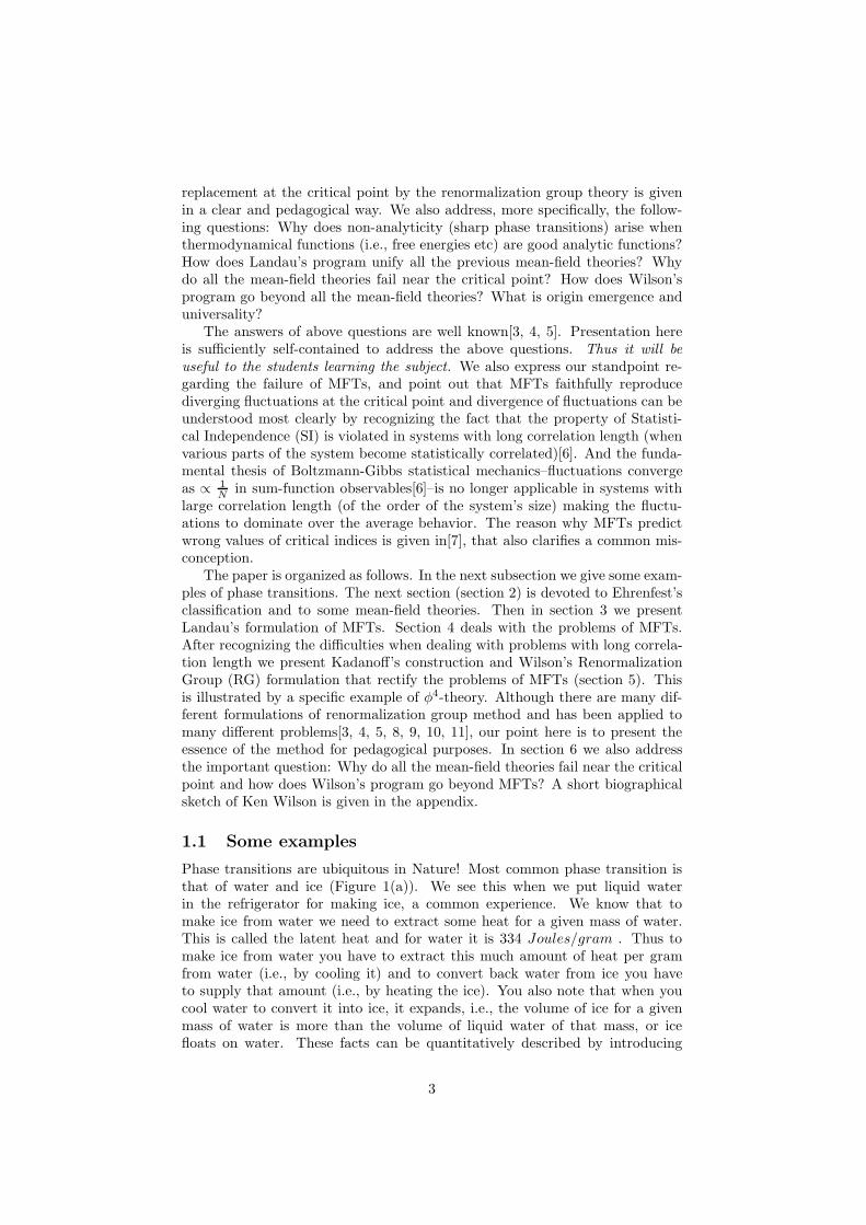
1.1 Some examples

Phase transitions are ubiquitous in Nature! Most common phase transition isthat of water and ice (Figure 1(a)). We see this when we put liquid waterin the refrigerator for making ice, a common experience. We know that tomake ice from water we need to extract some heat for a given mass of water.This is called the latent heat and for water it is 334 Joules/gram . Thus tomake ice from water you have to extract this much amount of heat per gramfrom water (i.e., by cooling it) and to convert back water from ice you haveto supply that amount (i.e., by heating the ice). You also note that when youcool water to convert it into ice, it expands, i.e., the volume of ice for a givenmass of water is more than the volume of liquid water of that mass, or icefloats on water. These facts can be quantitatively described by introducing

3

the thermodynamical free energy[22]. Discontinuity of its first order derivativeswith respect to thermodynamical parameters leads to above discontinuities. Wewill explain this in the section devoted to Ehrenfest’s classification.

0

Vapour

LiquidCritical Point

Solid

Triple Point

T

P

Melting Curve

Sublimation Curve

Vapour−pressure Curve

1 ATM

0.006 ATM

100 C0.01 C

.

(a) (b)

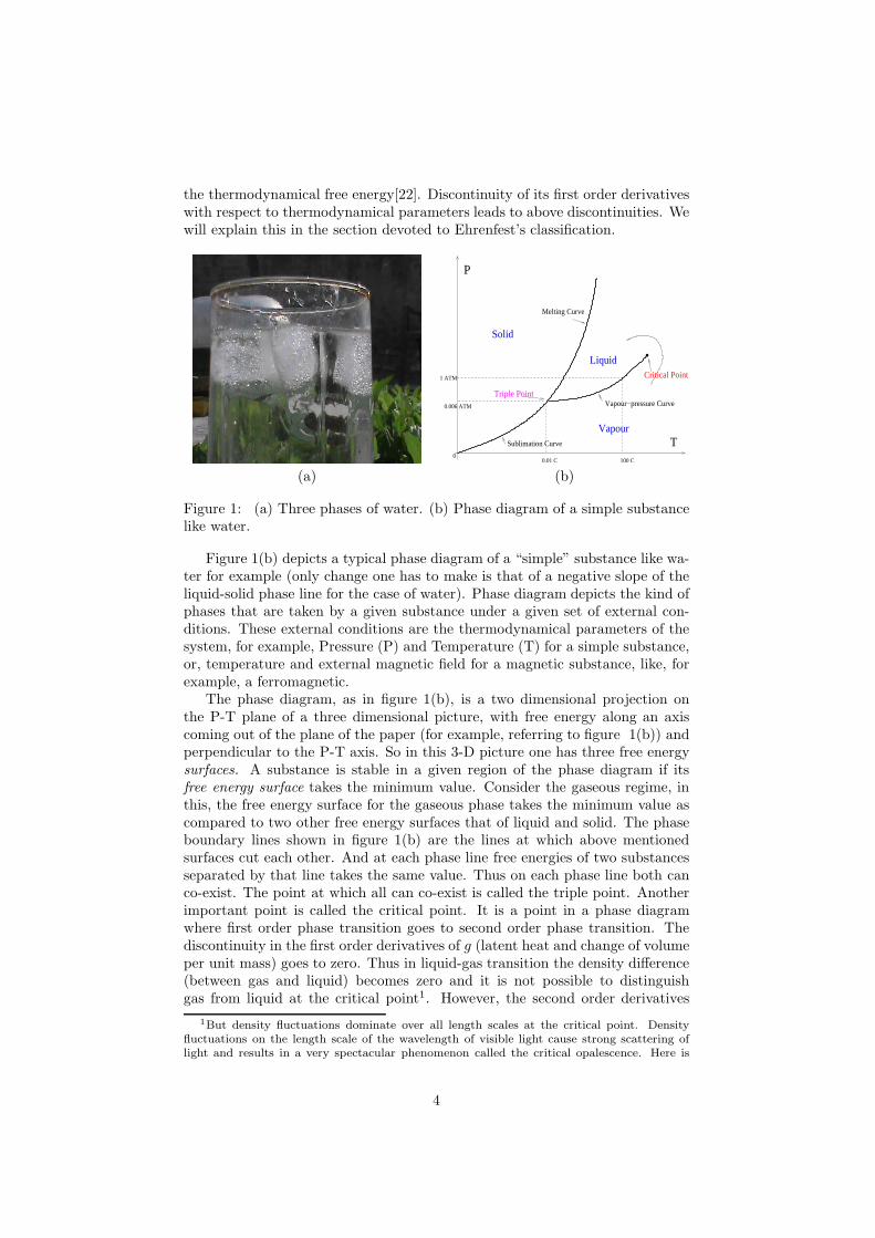
Figure 1: (a) Three phases of water. (b) Phase diagram of a simple substancelike water.

Figure 1(b) depicts a typical phase diagram of a “simple” substance like wa-ter for example (only change one has to make is that of a negative slope of theliquid-solid phase line for the case of water). Phase diagram depicts the kind ofphases that are taken by a given substance under a given set of external con-ditions. These external conditions are the thermodynamical parameters of thesystem, for example, Pressure (P) and Temperature (T) for a simple substance,or, temperature and external magnetic field for a magnetic substance, like, forexample, a ferromagnetic.

The phase diagram, as in figure 1(b), is a two dimensional projection onthe P-T plane of a three dimensional picture, with free energy along an axiscoming out of the plane of the paper (for example, referring to figure 1(b)) andperpendicular to the P-T axis. So in this 3-D picture one has three free energysurfaces. A substance is stable in a given region of the phase diagram if itsfree energy surface takes the minimum value. Consider the gaseous regime, inthis, the free energy surface for the gaseous phase takes the minimum value ascompared to two other free energy surfaces that of liquid and solid. The phaseboundary lines shown in figure 1(b) are the lines at which above mentionedsurfaces cut each other. And at each phase line free energies of two substancesseparated by that line takes the same value. Thus on each phase line both canco-exist. The point at which all can co-exist is called the triple point. Anotherimportant point is called the critical point. It is a point in a phase diagramwhere first order phase transition goes to second order phase transition. Thediscontinuity in the first order derivatives of g (latent heat and change of volumeper unit mass) goes to zero. Thus in liquid-gas transition the density difference(between gas and liquid) becomes zero and it is not possible to distinguishgas from liquid at the critical point1. However, the second order derivatives

1But density fluctuations dominate over all length scales at the critical point. Densityfluctuations on the length scale of the wavelength of visible light cause strong scattering oflight and results in a very spectacular phenomenon called the critical opalescence. Here is

4

of the Gibbs free energy remains discontinuous (see the section on Ehrenfest’sclassification).

2000 T (K)0

Artificial Diamonds 20

40

60

Pre

ssur

e G

Pa

4000

Liquid

Diamond

Graphite

(a) (b)

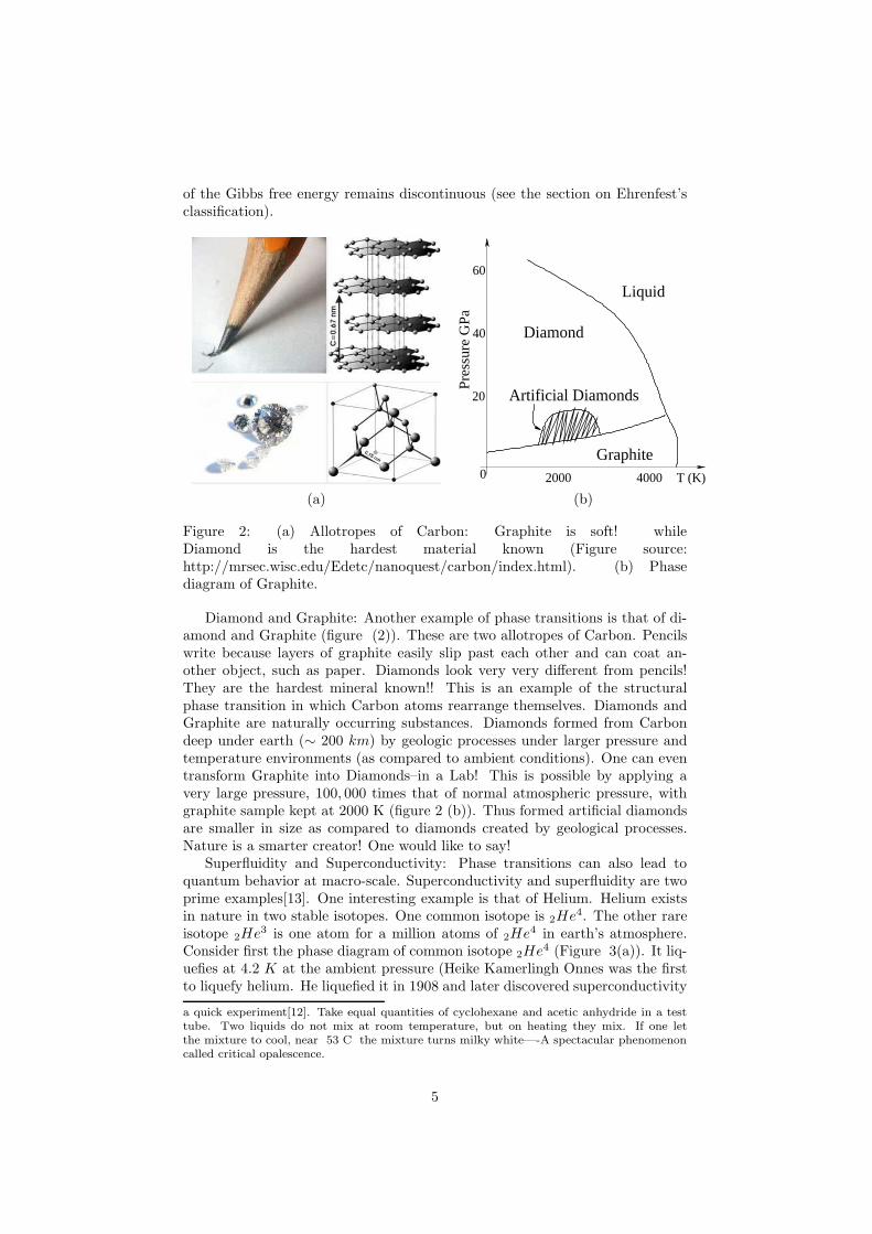
Figure 2: (a) Allotropes of Carbon: Graphite is soft! whileDiamond is the hardest material known (Figure source:http://mrsec.wisc.edu/Edetc/nanoquest/carbon/index.html). (b) Phasediagram of Graphite.

Diamond and Graphite: Another example of phase transitions is that of di-amond and Graphite (figure (2)). These are two allotropes of Carbon. Pencilswrite because layers of graphite easily slip past each other and can coat an-other object, such as paper. Diamonds look very very different from pencils!They are the hardest mineral known!! This is an example of the structuralphase transition in which Carbon atoms rearrange themselves. Diamonds andGraphite are naturally occurring substances. Diamonds formed from Carbondeep under earth (∼ 200 km) by geologic processes under larger pressure andtemperature environments (as compared to ambient conditions). One can eventransform Graphite into Diamonds–in a Lab! This is possible by applying avery large pressure, 100, 000 times that of normal atmospheric pressure, withgraphite sample kept at 2000 K (figure 2 (b)). Thus formed artificial diamondsare smaller in size as compared to diamonds created by geological processes.Nature is a smarter creator! One would like to say!

Superfluidity and Superconductivity: Phase transitions can also lead toquantum behavior at macro-scale. Superconductivity and superfluidity are twoprime examples[13]. One interesting example is that of Helium. Helium existsin nature in two stable isotopes. One common isotope is 2He

4. The other rareisotope 2He

3 is one atom for a million atoms of 2He4 in earth’s atmosphere.

Consider first the phase diagram of common isotope 2He4 (Figure 3(a)). It liq-

uefies at 4.2 K at the ambient pressure (Heike Kamerlingh Onnes was the firstto liquefy helium. He liquefied it in 1908 and later discovered superconductivity

a quick experiment[12]. Take equal quantities of cyclohexane and acetic anhydride in a testtube. Two liquids do not mix at room temperature, but on heating they mix. If one letthe mixture to cool, near 53 C the mixture turns milky white—-A spectacular phenomenoncalled critical opalescence.

5

0 TVapour

2He

(ATM)P

Pc

. ...

. ..

.... . . .

... .

0 K

SuperfluidNormal Liquid

4Common Isotope

lambda line

He IHe II

Solid

1 K 4 K3 K2 K

20

30

40

10

0

Liquid

TVapour

Solid

2He

3

1 K 2 K 3 K

30

10

20

40(ATM)P

Pc

Rare Isotope

0.18 0.49 K

. ...

. ..

.... . . .

... .

0.001 K

0 K

B

A

Superfluid

(a) (b)

Figure 3: Phase transitions in Helium. (a) Common Isotope 2He4, (b) The rare

isotope 2He3.

in Mercury in 1911). When cooled further ∼ 2.17 K it transforms to a newform of liquid (a new thermodynamical phase called the superfluid phase). Inthis phase liquid Helium flows without friction (zero viscosity) and becomes a“super-heat-conductor”. This superfluid phase of 2He

4 is also called the HeIIphase (the normal one is called HeI). Heat capacity shows an infinite disconti-nuity at 2.17 K (figure (4)). There is no latent heat involved2. The shape ofheat capacity curve resembles with that of a Greek letter lambda (λ). Thus itis also called the lambda-transition in liquid Helium literature. Liquid Heliumcan be made solid by applying a pressure of 25 atm for temperature less than 2K. Higher temperatures require higher pressure for solidification (figure 3 (a)).Interestingly it does not have a triple point! The rare isitope 2He

3 behaves

0 K 1 K 4 K3 K2 KT

transition inλ−

He2

4

SuperfluidHe II

C (cal/g/deg)

4

3

2

2.172 K

Liquid He I

Figure 4: The lambda-transition in common Helium.

exotically (figure 3(b)). If you start from a very low temperature, say 0.0001 K,

2But it is not the second order phase transition! see Ehrenfest’s classification in the nextsection.

6

Hea

t Cap

acit

y

Tc T(K)

−1.7 T /Te c

c

c T

c

Figure 5: Superconducting phase transition. (a) Heat capacity show a finite dis-continuity at Tc, (b) Superconducting substances show Meissner effect (Image:public domain/Wikimedia Commons.).

with a sample of 2He3 at 30 atm pressure, you first have liquid Helium. On

reaching 0.18 K it solidifies! It remains solid upto 0.49 K and again turns liquidfor higher temperatures. This behavior of the rare isotope of Helium is quiteunusual (as common solids remain solid with reducing temperature!).

The superfluidity of the normal isotope 2He4 is due to the Bose-Einstein

condensation below the condensation temperature ∼ 2.17 K. As 2He4 atoms

are bosons they condense into the ground state with order parameter (the con-densate wavefunction) as ρeφ. Where ρ is the superfluid density and φ is phaseof the wave function. All the observed properties can be understood using two-fluid picture (see for details[14]). The reason why Helium remains liquid downto the lowest temperatures achievable at normal pressure is the large amplitudesof the zero-point quantum oscillations that disrupt the crystalline order.

The case of the rare isotope is much more interesting. As 2He3 atoms are

fermions they cannot show BEC directly and thus superfuildity. But experimen-tally superfuildity has been seen. The reason for superfluidity in the rare iso-tope is the formation of Cooper pairs between Helium atoms much like the BCS(Bardeen-Cooper-Schrieffer) theory of superconductivity[15], but with impor-tant differences: As there is no crystalline lattice, phonons are not operative informing Cooper pairs (in contrast to simple metals explainable by BCS theory).The origin of Cooper pairing in the rare isotope is magnetic and Coopers pairsresides in higher angular momentum states with internal degrees-of-freedom (seeAnderson-Morel[16]).

Superconductivity is an another example that show macroscopic quantumeffects. First discovered by Heike Kamerlingh Onnes in 1911, it took aboutfifty years of theoretical efforts and finally the microscopic understanding camewith BCS theory of superconductivity in 1957[15]. Loosely speaking the basis ofsuperconductivity is the Bose-Einstein condensation of Cooper pairs formed dueto mutual attractive interaction mediated by the exchange of lattice phonons.The important difference between rare isotope of Helium and superconductivityin simple metals is that the size of a Cooper pair in metals is much greater thanmean particle separation (∼ 1000 times the lattice constant) while in Heliumit is like forming a bosonic molecule by two fermionic atoms (the size of the

7

Cooper pair is mean particle separation). BCS theory quantitatively accountfor many observed properties of simple superconductors (excluding Cupratesuperconductors[13, 17]).

Magnetism of Iron: Iron loses its magnetic properties above 770 C (theCurie temperature). What happens is that due to thermal agitation the orderedarrangement of electronic spins becomes unstable. The origin of magnetism inIron is due to a dual role played by d-band electrons[18, 19]. They participate inmetallic bounding as well as act like localized spins. Iron drives its magnetismfrom electron-electron repulsive Coloumb interaction due to which they avoideach other in real space and that is effectively executed by keeping spins in thesame direction. This a rough picture (see for more accurate and quantitativeanalysis[19]).

Cosmological Phase Transition: The origin of SU3, Isospin, and Parity! Ithas been postulated (after the discovery of Hubble expansion) that when ouruniverse was very young (only sub-pico seconds of age) after the Big-Bang,our universe underwent a phase transition from that high energy scale–calledthe Cosmological phase transition. Below that high energy scale the electroweaksymmetry is broken. This the phase transition of vacuum itself in which vacuumexpectation value of a scalar field takes non-zero value[20]. This is intimatelyconnected to the Higgs mechanism[21].

The above are some examples of phase transitions. Obviously, there aremany more examples. The above are sufficient for our purpose of illustratingthe mean-field theories and renormalization group. Before we discuss the MFTswe first review the work of Ehrenfest on the classifications of phase transitions.

2 Phase transitions without Landau’s paradigm

2.1 Ehrenfest’s classification of phase transitions

Paul Ehrenfest (1880-1933)3 classified various phase transitions in 1933 accord-ing to the behavior of the derivatives of the Gibbs free energy (unfortunately,later that year he killed himself as he was suffering from severe depression).

Figure 6: Ehrenfest andhis son with Einstein1920.

According to this scheme, the order of a phase transi-tion is given by the order of the discontinuous deriva-tive of Gibbs free energy. On the line separatingthe two phases (say, in the liquid-gas transition) theGibbs free energies per unit mass g(T, P ) of the twophases take the same value. On the left of the line, gis less for the liquid, and on the right of it it is lessfor the gas. By definition[22]: g(T, P ) = U −Ts+Pvor dg = −sdT + vdP with

Entropy/mass = s = −∂g

∂T|P .

V olume/mass = v =∂g

∂P|T

First order phase transitions are those in which first order derivatives of theGibbs’ Free energy are discontinuous: i.e., if the above derivatives are discon-

3He was a student of Ludwig Boltzmann.

8

tinuous. If we cross the liquid-solid line vertically in up direction (at constanttemperature, see figure 1 (b)) clearly:

∂gl∂P

|T >∂gs∂P

|T

As the system goes from liquid stability to solid stability (an experimental fact!).This implies that:

vl =∂gl∂P

|T > vs =∂gs∂P

|T

In other words, for a given mass, volume of the liquid phase is more than thatof the solid phase, or, substances expand on melting!4

If we cross the liquid-gas line horizontally (ref. figure 1(b)) from left to right(at constant pressure) clearly:

∂gs∂T

|P >∂gl∂T

|P

As system goes from solid stability to liquid stability (again an experimentalfact!). Above implies that

−ss > −sl

or

ss < sl, ⇒ql − qsT

> 0.

Where ql − qs = l is called the latent heat of solid-to-liquid transition, whichis positive! as it should be! Thus heat must be absorbed from solid to liquidtransition. Examples of first order are: Solid-liquid-vapor, transitions in simplefluids, allotropic transformations (like diamond graphite) etc.

For the second order phase transitions, first order derivative of Gibbs freeenergy, i.e., v, s, are continuous, but the second order derivatives, i.e., heatcapacity c, and compressibility κ are discontinuous. Thus no latent heat andvolume change occur during a second order phase transition. But in a secondorder transition, heat capacity and compressibility show finite discontinuity. Anideal second order transition is the superconducting transition in zero magneticfield[22].

Phase transition in liquid Helium is not second order (as the discontinuityin heat capacity is infinite). This is a special transition called the λ−transition.

Above is called the Ehrenfest’s classification scheme. One can define higherorder phase transitions along these lines (third and higher order derivatives ofthe Gibbs free energy), but those are seldom observed in practice. Ehrenfest’sscheme is based on the fundamental thermodynamical principle: the phase ofminimum free energy is the stable one[22]. From this it derives other propertiesof phase transitions like latent heat, volume changes etc. Importantly, it doesnot provide more fundamental statistical mechanical formulation of the phasetransition behavior. We will see in the next section that MFTs are the firststeps in these directions.

We will also see that with the Landau’s paradigm above scheme of Ehren-fests’ can be nicely re-interpreted by using the order parameter concept.

4Note that the case of water is opposite (ice is lighter) as the ice-water (solid-liquid) linehas negative slop.

9

2.2 The Mean-Field Theories(MFTs)

The above is the macroscopic way of understanding/classifying the phase tran-sitions without any microscipic (atomic/molecular) point of view. Attemptsto understand the laws of heat from the microscipic (atomic/molecular) per-spective resulted in the science of statistical mechanics and Ludwig Boltzamnn(1844-1906) was the pioneer[23]. Similar to this philosophy, to understand phasetransition phenomena from atomic/moleculaer perspective, early attempts weremade by van der Waals5.

Thus the credit of first mean-field theory goes to van der Waals’[1]. Van derWaals was interested in the notion of continuity of matter, namely, how a gaseoussubstance, on cooling, transforms into a liquid while chemically, at molecularlevel things remain intact6. His main concern was the ideal gas equation andthe problems of the Boyle’s law. Here is a rough sketch of his argument.

We know that the ideal gas equation

PV = NkBT = nRT

shows no phase transition for obvious reasons (due to the neglect of inter-molecular forces). In contrast, real gases at low temperature and high pressuredeviate markedly from the ideal gas behavior. To see this, let V 0

m be the molarvolume (volume per mole) of an ideal gas:

pV 0m = RT.

Define the compression factor Z at a temperature T for a real gas (PVm = RT ):

Z =VmV 0m

=pVmRT

.

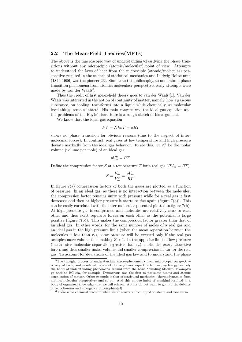
In figure 7(a) compression factors of both the gases are plotted as a functionof pressure. In an ideal gas, as there is no interaction between the molecules,the compression factor remains unity with pressure while for a real gas it firstdecreases and then at higher pressure it starts to rise again (figure 7(a)). Thiscan be easily correlated with the inter-molecular potential plotted in figure 7(b).At high pressure gas is compressed and molecules are relatively near to eachother and thus exert repulsive forces on each other as the potential is largepositive (figure 7(b)). This makes the compression factor greater than that ofan ideal gas. In other words, for the same number of moles of a real gas andan ideal gas in the high pressure limit (when the mean separation between themolecules is less than rc), same pressure will be exerted only if the real gasoccupies more volume thus making Z > 1. In the opposite limit of low pressure(mean inter molecular separation greater than rc), molecules exert attractiveforces and thus smaller molar volume and smaller compression factor for the realgas. To account for deviations of the ideal gas law and to understand the phase

5The thought process of understanding macro-phenomema from microscopic perspectiveis very old one, and is related to one of the very basic aspect of human psychology, namelythe habit of understanding phenomena around from the basic “building blocks”. Examplesgo back to BC era, for example, Democritus was the first to postulate atoms and atomicconstitution of matter. Other example is that of statistical mechanics (thermodynamics fromatomic/molecular perspective) and so on. And this unique habit of mankind resulted in abody of organized knowledge that we call science. Author do not want to go into the debatesof reductionism and emergence philosophies[24]

6There is no chemical reaction when water converts from liquid to steam and vice versa.

10

0

Com

pres

sion F

acto

r, Z

200 400 600p/atm

Real Gas ( CH )4

Meth

ane

Z=1

Perfect gas

T=0 C

Pote

ntia

l ene

rgy

of in

tera

ctio

n

Separationrc

Figure 7: (a) Behavior of the compression factor for an ideal gas as comparedwith a real gas. (b) Inter molecular force as a function of separation in a realgas.

VReal gas isotherms

V

PP1

2

3

12

3

van der Waals isotherms

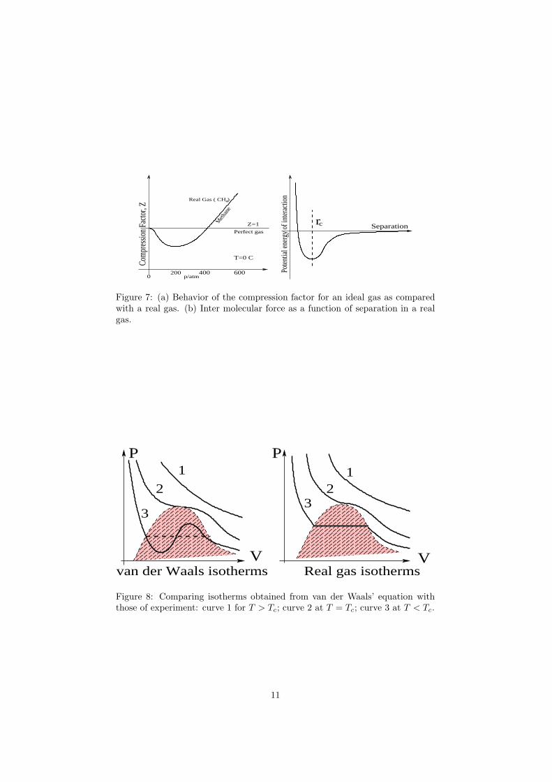
Figure 8: Comparing isotherms obtained from van der Waals’ equation withthose of experiment: curve 1 for T > Tc; curve 2 at T = Tc; curve 3 at T < Tc.

11

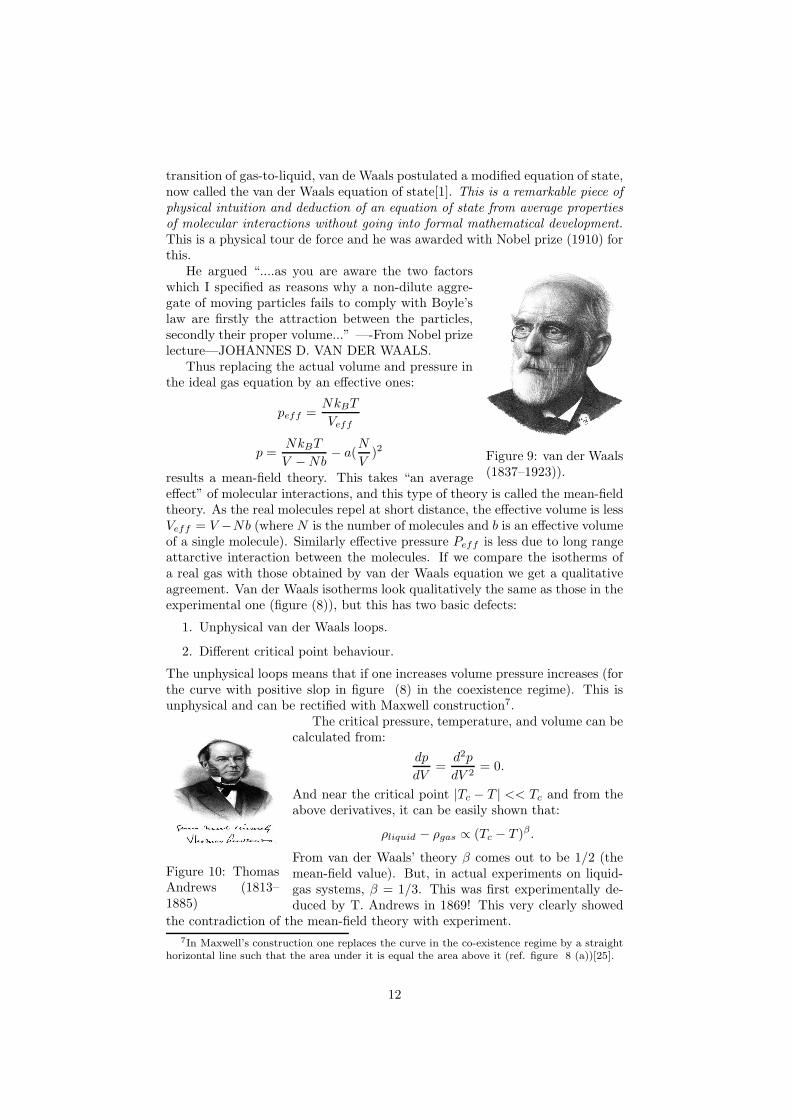
transition of gas-to-liquid, van de Waals postulated a modified equation of state,now called the van der Waals equation of state[1]. This is a remarkable piece ofphysical intuition and deduction of an equation of state from average propertiesof molecular interactions without going into formal mathematical development.This is a physical tour de force and he was awarded with Nobel prize (1910) forthis.

Figure 9: van der Waals(1837–1923)).

He argued “....as you are aware the two factorswhich I specified as reasons why a non-dilute aggre-gate of moving particles fails to comply with Boyle’slaw are firstly the attraction between the particles,secondly their proper volume...” —-From Nobel prizelecture—JOHANNES D. VAN DER WAALS.

Thus replacing the actual volume and pressure inthe ideal gas equation by an effective ones:

peff =NkBT

Veff

p =NkBT

V −Nb− a(

N

V)2

results a mean-field theory. This takes “an averageeffect” of molecular interactions, and this type of theory is called the mean-fieldtheory. As the real molecules repel at short distance, the effective volume is lessVeff = V −Nb (where N is the number of molecules and b is an effective volumeof a single molecule). Similarly effective pressure Peff is less due to long rangeattarctive interaction between the molecules. If we compare the isotherms ofa real gas with those obtained by van der Waals equation we get a qualitativeagreement. Van der Waals isotherms look qualitatively the same as those in theexperimental one (figure (8)), but this has two basic defects:

1. Unphysical van der Waals loops.

2. Different critical point behaviour.

The unphysical loops means that if one increases volume pressure increases (forthe curve with positive slop in figure (8) in the coexistence regime). This isunphysical and can be rectified with Maxwell construction7.

Figure 10: ThomasAndrews (1813–1885)

The critical pressure, temperature, and volume can becalculated from:

dp

dV=

d2p

dV 2= 0.

And near the critical point |Tc − T | << Tc and from theabove derivatives, it can be easily shown that:

ρliquid − ρgas ∝ (Tc − T )β.

From van der Waals’ theory β comes out to be 1/2 (themean-field value). But, in actual experiments on liquid-gas systems, β = 1/3. This was first experimentally de-duced by T. Andrews in 1869! This very clearly showed

the contradiction of the mean-field theory with experiment.

7In Maxwell’s construction one replaces the curve in the co-existence regime by a straighthorizontal line such that the area under it is equal the area above it (ref. figure 8 (a))[25].

12

We will see that this discrepancy is not specific to van der Waals theory buta basic defect of all such theories called the MFTs at the critical point. It tookabout 100 years for the resolution of this discrepancy!! This happened in thehands of K. G. Wilson in early 70s. The culprit is non-negligible fluctuations(density fluctuations in this liquid-gas case) at all length scales that invalidatesthe application of the mean-field theory itself[7].

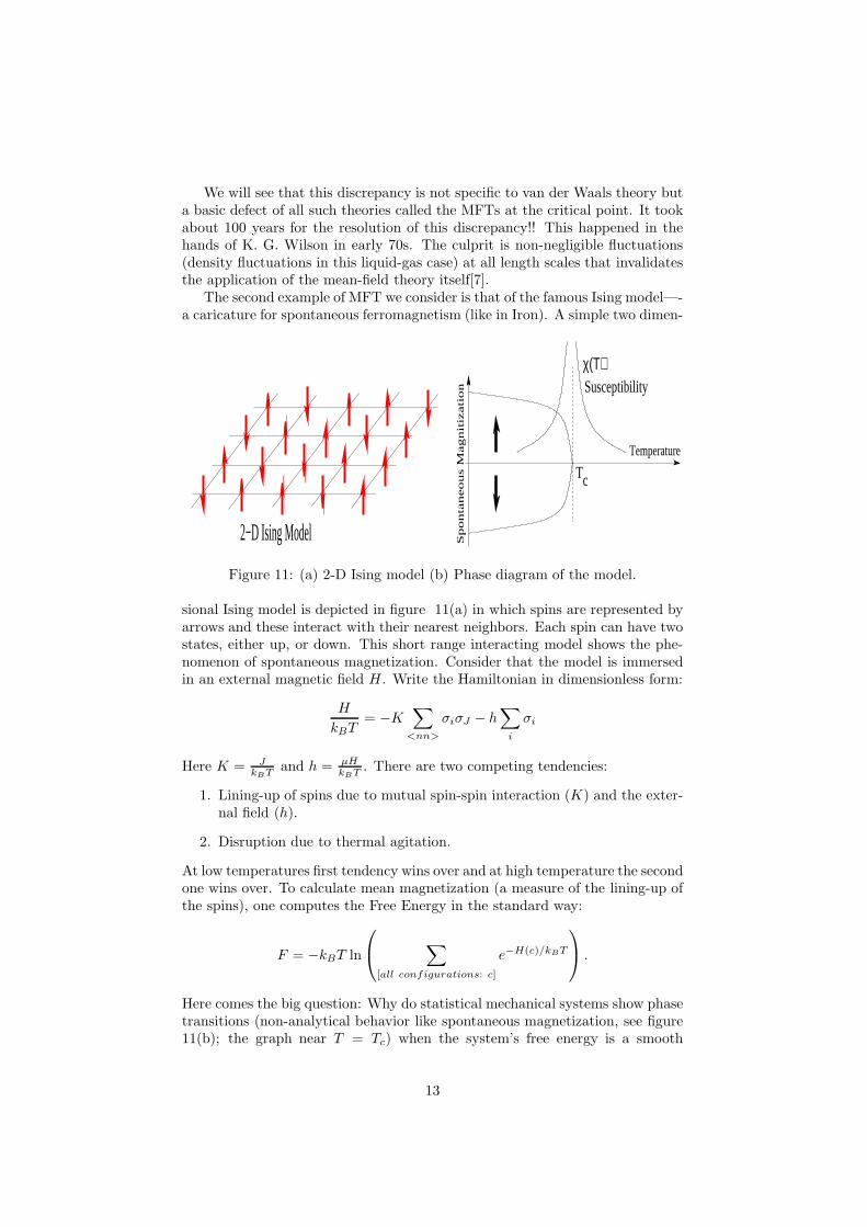
The second example of MFT we consider is that of the famous Ising model—-a caricature for spontaneous ferromagnetism (like in Iron). A simple two dimen-

2−D Ising Model

χ(Τ)Susceptibility

Tc

TemperatureS

ponta

neous M

agnit

izati

on

Figure 11: (a) 2-D Ising model (b) Phase diagram of the model.

sional Ising model is depicted in figure 11(a) in which spins are represented byarrows and these interact with their nearest neighbors. Each spin can have twostates, either up, or down. This short range interacting model shows the phe-nomenon of spontaneous magnetization. Consider that the model is immersedin an external magnetic field H . Write the Hamiltonian in dimensionless form:

H

kBT= −K

∑

<nn>

σiσJ − h∑

i

σi

Here K = JkBT and h = µH

kBT . There are two competing tendencies:

1. Lining-up of spins due to mutual spin-spin interaction (K) and the exter-nal field (h).

2. Disruption due to thermal agitation.

At low temperatures first tendency wins over and at high temperature the secondone wins over. To calculate mean magnetization (a measure of the lining-up ofthe spins), one computes the Free Energy in the standard way:

F = −kBT ln

∑

[all configurations: c]

e−H(c)/kBT

.

Here comes the big question: Why do statistical mechanical systems show phasetransitions (non-analytical behavior like spontaneous magnetization, see figure11(b); the graph near T = Tc) when the system’s free energy is a smooth

13

function of temperature and of system’s parameters (an analytical function)?Sum of smooth exponentials is a smooth function!

The origin of non-analyticity (like spontaneous magnetization) is in the ther-modynamical limit (infinite system size!): Larger the system size sharper is thetransition: As real phase transitions involve thermodynamical systems havingvery large number of particles of the order of Avogadro number, transitionsappear infinitely sharp to human perception! This has been dubbed as “ex-tended singularity theorem” by Leo Kadanoff or better one can say “extendedsingularity conjecture”[4]. As the proof exists only in one special case[26].

Mean-field theory for the Ising model is done in usual way[4, 27, 28]:

1. First, consider that just one spin is immersed in magnetic field (that cantake two values: +1 (up-spin, say), and −1 (down-spin)). Thermal expec-tation value of the spin is:

〈σ〉 =

∑

σ=±1 σehσ

∑

σ=±1 ehσ

= tanh(h).

2. Second, when our test spin is interacting with many neighboring spins, allimmersed in magnetic field:

〈σ〉 =

∑

σ=±1 σeheffσ

∑

σ=±1 eheffσ

= tanh(h+K∑

<nn>

σi) ≃ tanh(heff ).

heff = h+ effective field due to other spins = h+ zK 〈σ〉.

Here the exact field K∑

<nn> σi due to near-neighbor spins is replacedby the effective field ∼ zK〈σ〉 (z is called the coordination number, = 4in 2D). This constitutes the mean-field approximation.

Thus in MFT: 〈σ〉 = tanh(h + zK〈σ〉). To see what values 〈σ〉 can take,one must solve this self-consistently. As K ∝ 1

T it turns out that zK = Tc

T(where Tc is the critical temperature). In zero external field h = 0 the equation〈σ〉 = tanh(Tc

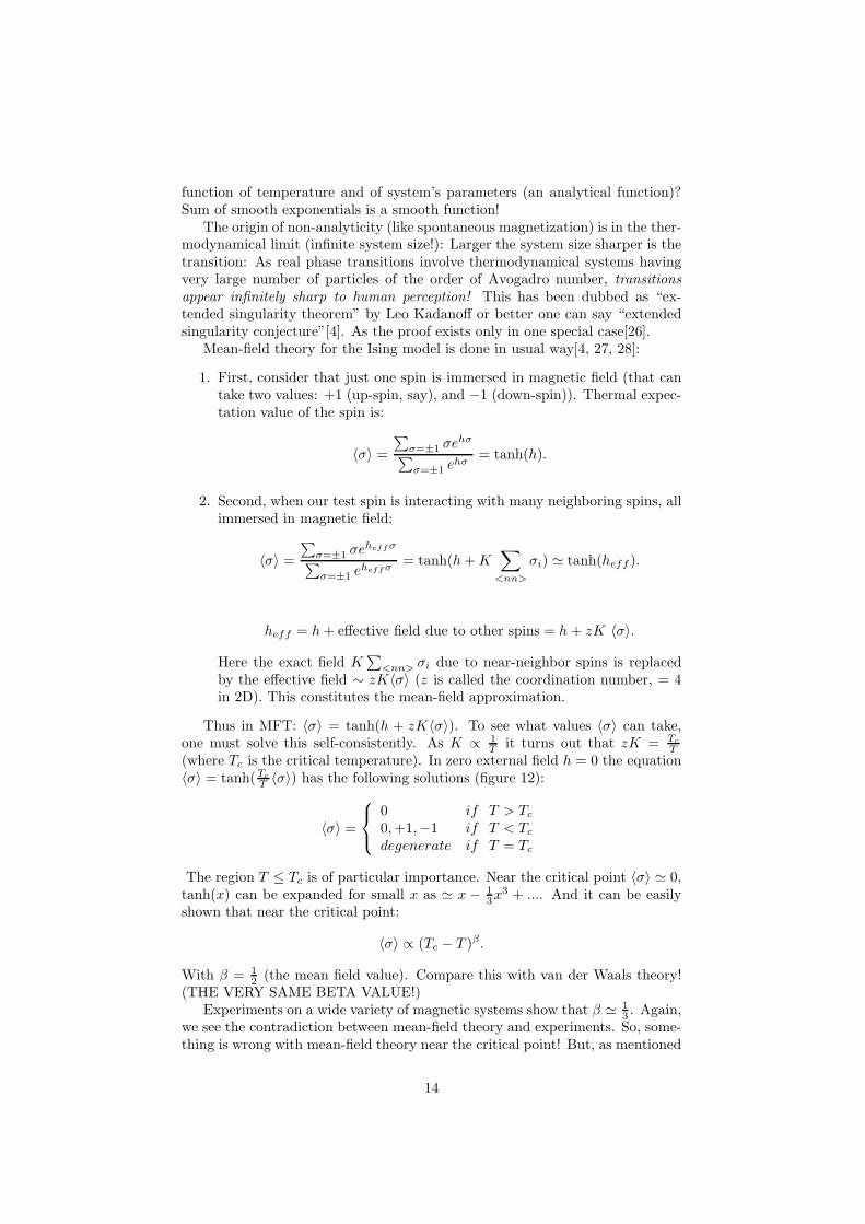
T 〈σ〉) has the following solutions (figure 12):

〈σ〉 =

0 if T > Tc0,+1,−1 if T < Tcdegenerate if T = Tc

The region T ≤ Tc is of particular importance. Near the critical point 〈σ〉 ≃ 0,tanh(x) can be expanded for small x as ≃ x − 1

3x3 + .... And it can be easily

shown that near the critical point:

〈σ〉 ∝ (Tc − T )β.

With β = 12 (the mean field value). Compare this with van der Waals theory!

(THE VERY SAME BETA VALUE!)Experiments on a wide variety of magnetic systems show that β ≃ 1

3 . Again,we see the contradiction between mean-field theory and experiments. So, some-thing is wrong with mean-field theory near the critical point! But, as mentioned

14

T=TT<TT>Tc c ctanh

Figure 12: Solutions of the zero field mean-field equation.

before, solution comes much later. However, the great merit of MFTs is thatthey qualitatively explain the emergence of phases below Tc (refer to the middlegraph in figure (12)). One can show that the free energy for 〈σ〉 = 0 phase isgreater than the other phases with non-zero 〈σ〉, and the phase with minimumfree energy is the phase that is realized in a thermodynamical system. Thus onehas non-zero 〈σ〉 for temperature less than the critical temperature (figure 11).

3 Landau’s paradigm: symmetry breaking andthe order parameter concept

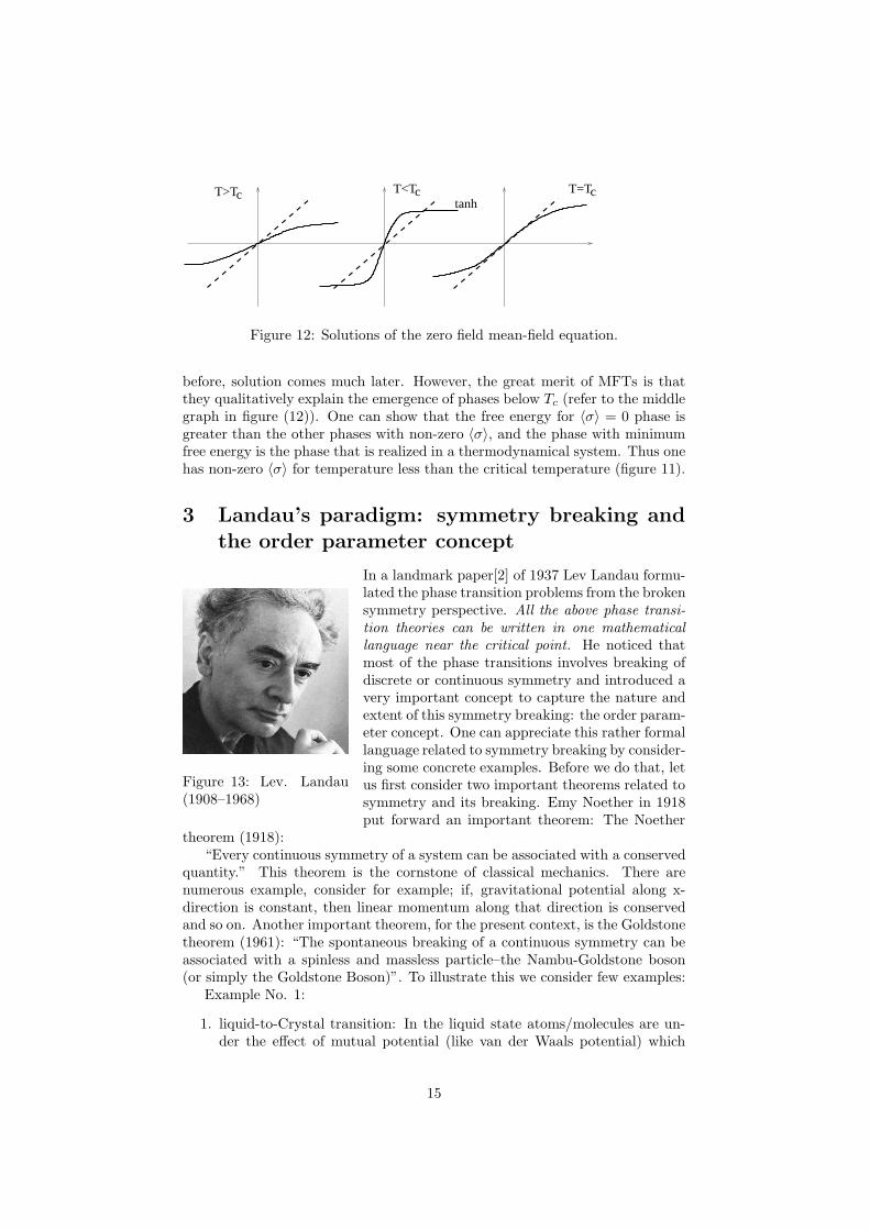
Figure 13: Lev. Landau(1908–1968)

In a landmark paper[2] of 1937 Lev Landau formu-lated the phase transition problems from the brokensymmetry perspective. All the above phase transi-tion theories can be written in one mathematicallanguage near the critical point. He noticed thatmost of the phase transitions involves breaking ofdiscrete or continuous symmetry and introduced avery important concept to capture the nature andextent of this symmetry breaking: the order param-eter concept. One can appreciate this rather formallanguage related to symmetry breaking by consider-ing some concrete examples. Before we do that, letus first consider two important theorems related tosymmetry and its breaking. Emy Noether in 1918put forward an important theorem: The Noether

theorem (1918):“Every continuous symmetry of a system can be associated with a conserved

quantity.” This theorem is the cornstone of classical mechanics. There arenumerous example, consider for example; if, gravitational potential along x-direction is constant, then linear momentum along that direction is conservedand so on. Another important theorem, for the present context, is the Goldstonetheorem (1961): “The spontaneous breaking of a continuous symmetry can beassociated with a spinless and massless particle–the Nambu-Goldstone boson(or simply the Goldstone Boson)”. To illustrate this we consider few examples:

Example No. 1:

1. liquid-to-Crystal transition: In the liquid state atoms/molecules are un-der the effect of mutual potential (like van der Waals potential) which

15

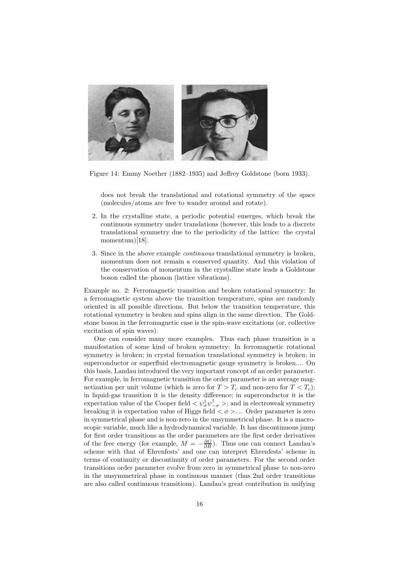
Figure 14: Emmy Noether (1882–1935) and Jeffrey Goldstone (born 1933).

does not break the translational and rotational symmetry of the space(molecules/atoms are free to wander around and rotate).

2. In the crystalline state, a periodic potential emerges, which break thecontinuous symmetry under translations (however, this leads to a discretetranslational symmetry due to the periodicity of the lattice: the crystalmomentum)[18].

3. Since in the above example continuous translational symmetry is broken,momentum does not remain a conserved quantity. And this violation ofthe conservation of momentum in the crystalline state leads a Goldstoneboson called the phonon (lattice vibrations).

Example no. 2: Ferromagnetic transition and broken rotational symmetry: Ina ferromagnetic system above the transition temperature, spins are randomlyoriented in all possible directions. But below the transition temperature, thisrotational symmetry is broken and spins align in the same direction. The Gold-stone boson in the ferromagnetic case is the spin-wave excitations (or, collectiveexcitation of spin waves).

One can consider many more examples. Thus each phase transition is amanifestation of some kind of broken symmetry: In ferromagnetic rotationalsymmetry is broken; in crystal formation translational symmetry is broken; insuperconductor or superfluid electromagnetic gauge symmetry is broken.... Onthis basis, Landau introduced the very important concept of an order parameter.For example, in ferromagnetic transition the order parameter is an average mag-netization per unit volume (which is zero for T > Tc and non-zero for T < Tc);in liquid-gas transition it is the density difference; in superconductor it is theexpectation value of the Cooper field < ψ†

σψ†−σ >; and in electroweak symmetry

breaking it is expectation value of Higgs field < φ >.... Order parameter is zeroin symmetrical phase and is non-zero in the unsymmetrical phase. It is a macro-scopic variable, much like a hydrodynamical variable. It has discontinuous jumpfor first order transitions as the order parameters are the first order derivativesof the free energy (for example, M = − ∂G

∂H ). Thus one can connect Landau’sscheme with that of Ehrenfests’ and one can interpret Ehrenfests’ scheme interms of continuity or discontinuity of order parameters. For the second ordertransitions order parameter evolve from zero in symmetrical phase to non-zeroin the unsymmetrical phase in continuous manner (thus 2nd order transitionsare also called continuous transitions). Landau’s great contribution in unifying

16

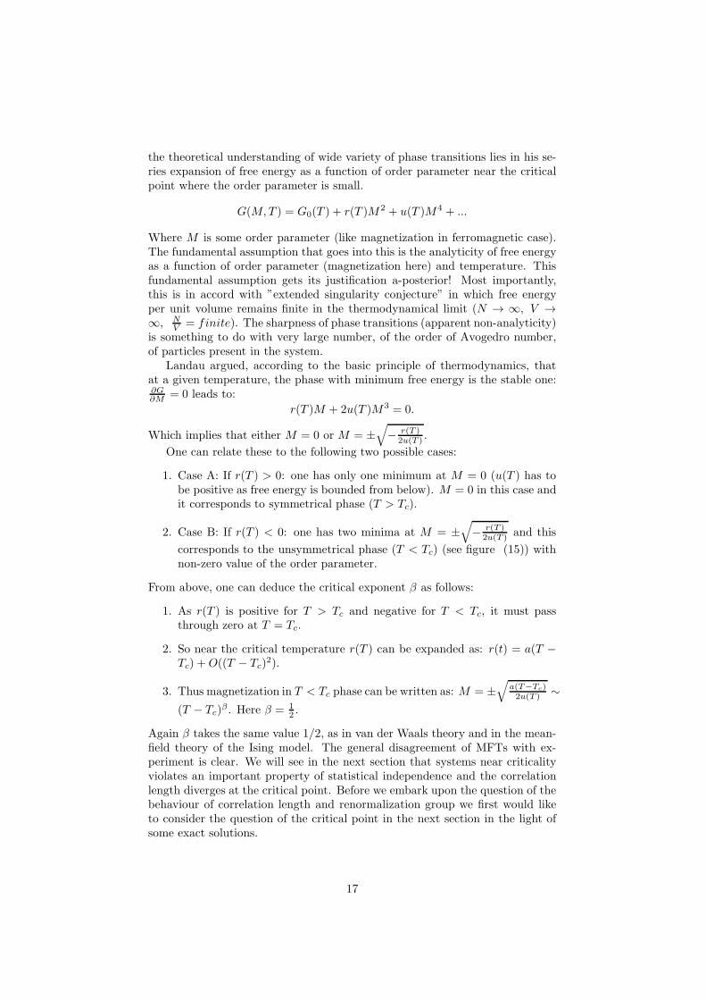
the theoretical understanding of wide variety of phase transitions lies in his se-ries expansion of free energy as a function of order parameter near the criticalpoint where the order parameter is small.

G(M,T ) = G0(T ) + r(T )M2 + u(T )M4 + ...

Where M is some order parameter (like magnetization in ferromagnetic case).The fundamental assumption that goes into this is the analyticity of free energyas a function of order parameter (magnetization here) and temperature. Thisfundamental assumption gets its justification a-posterior! Most importantly,this is in accord with ”extended singularity conjecture” in which free energyper unit volume remains finite in the thermodynamical limit (N → ∞, V →∞, N

V = finite). The sharpness of phase transitions (apparent non-analyticity)is something to do with very large number, of the order of Avogedro number,of particles present in the system.

Landau argued, according to the basic principle of thermodynamics, thatat a given temperature, the phase with minimum free energy is the stable one:∂G∂M = 0 leads to:

r(T )M + 2u(T )M3 = 0.

Which implies that either M = 0 or M = ±√

− r(T )2u(T ) .

One can relate these to the following two possible cases:

1. Case A: If r(T ) > 0: one has only one minimum at M = 0 (u(T ) has tobe positive as free energy is bounded from below). M = 0 in this case andit corresponds to symmetrical phase (T > Tc).

2. Case B: If r(T ) < 0: one has two minima at M = ±√

− r(T )2u(T ) and this

corresponds to the unsymmetrical phase (T < Tc) (see figure (15)) withnon-zero value of the order parameter.

From above, one can deduce the critical exponent β as follows:

1. As r(T ) is positive for T > Tc and negative for T < Tc, it must passthrough zero at T = Tc.

2. So near the critical temperature r(T ) can be expanded as: r(t) = a(T −Tc) +O((T − Tc)

2).

3. Thus magnetization in T < Tc phase can be written as: M = ±√

a(T−Tc)2u(T ) ∼

(T − Tc)β . Here β = 1

2 .

Again β takes the same value 1/2, as in van der Waals theory and in the mean-field theory of the Ising model. The general disagreement of MFTs with ex-periment is clear. We will see in the next section that systems near criticalityviolates an important property of statistical independence and the correlationlength diverges at the critical point. Before we embark upon the question of thebehaviour of correlation length and renormalization group we first would liketo consider the question of the critical point in the next section in the light ofsome exact solutions.

17

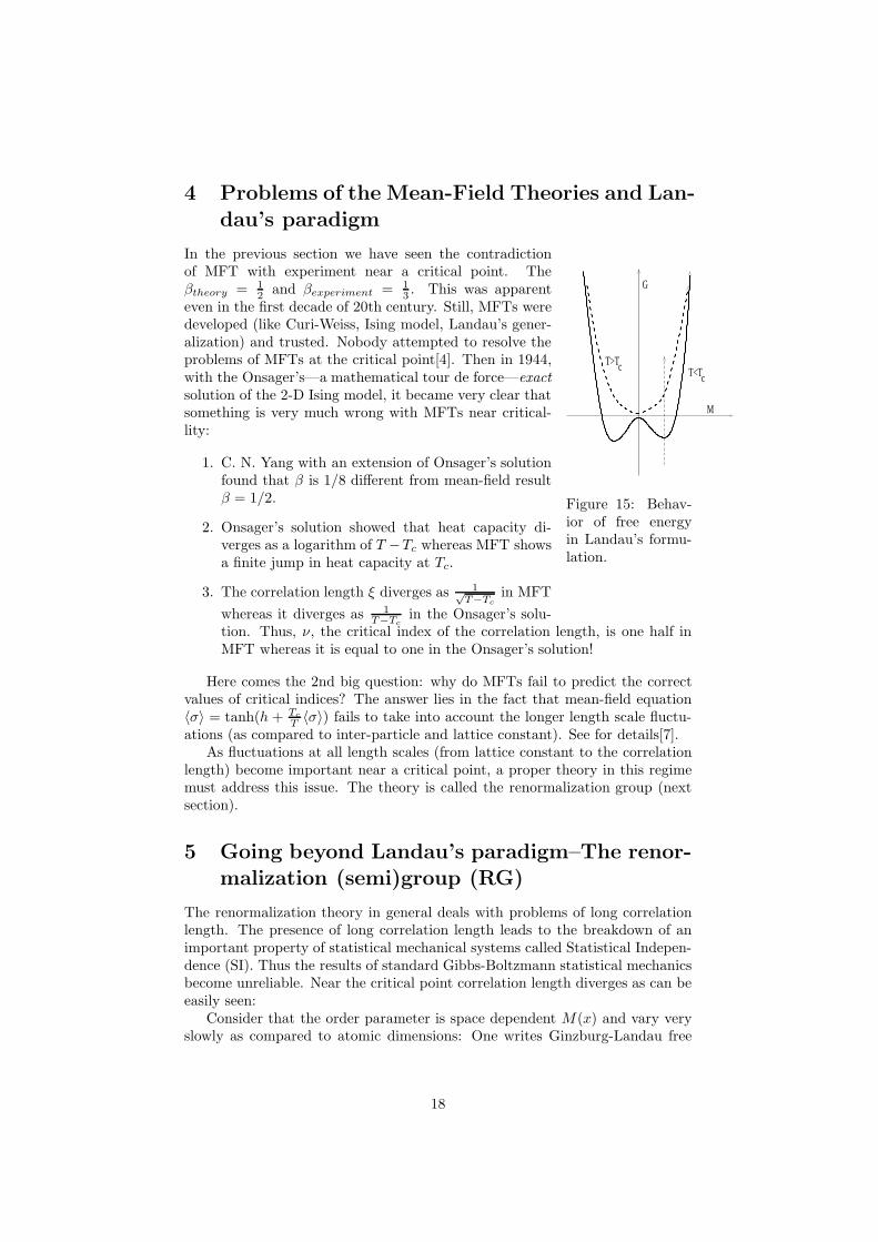
4 Problems of the Mean-Field Theories and Lan-

dau’s paradigm

T<TT>T

cc

G

M

Figure 15: Behav-ior of free energyin Landau’s formu-lation.

In the previous section we have seen the contradictionof MFT with experiment near a critical point. Theβtheory = 1

2 and βexperiment = 13 . This was apparent

even in the first decade of 20th century. Still, MFTs weredeveloped (like Curi-Weiss, Ising model, Landau’s gener-alization) and trusted. Nobody attempted to resolve theproblems of MFTs at the critical point[4]. Then in 1944,with the Onsager’s—a mathematical tour de force—exactsolution of the 2-D Ising model, it became very clear thatsomething is very much wrong with MFTs near critical-lity:

1. C. N. Yang with an extension of Onsager’s solutionfound that β is 1/8 different from mean-field resultβ = 1/2.

2. Onsager’s solution showed that heat capacity di-verges as a logarithm of T −Tc whereas MFT showsa finite jump in heat capacity at Tc.

3. The correlation length ξ diverges as 1√T−Tc

in MFT

whereas it diverges as 1T−Tc

in the Onsager’s solu-tion. Thus, ν, the critical index of the correlation length, is one half inMFT whereas it is equal to one in the Onsager’s solution!

Here comes the 2nd big question: why do MFTs fail to predict the correctvalues of critical indices? The answer lies in the fact that mean-field equation〈σ〉 = tanh(h + Tc

T 〈σ〉) fails to take into account the longer length scale fluctu-ations (as compared to inter-particle and lattice constant). See for details[7].

As fluctuations at all length scales (from lattice constant to the correlationlength) become important near a critical point, a proper theory in this regimemust address this issue. The theory is called the renormalization group (nextsection).

5 Going beyond Landau’s paradigm–The renor-malization (semi)group (RG)

The renormalization theory in general deals with problems of long correlationlength. The presence of long correlation length leads to the breakdown of animportant property of statistical mechanical systems called Statistical Indepen-dence (SI). Thus the results of standard Gibbs-Boltzmann statistical mechanicsbecome unreliable. Near the critical point correlation length diverges as can beeasily seen:

Consider that the order parameter is space dependent M(x) and vary veryslowly as compared to atomic dimensions: One writes Ginzburg-Landau free

18

energy functional[3]:

F =

∫

d3x{(∇M(x))2 + r(T )M(x)2 + u(T )M(x)4 −B(x)M(x)}.

Correlation length ξ is defined as the distance over which the effect of a testspin extends out to other nearby spins. To calculate ξ consider B(x) = B0δ

3(x)(magnetic field in a narrow region of space). Neglect the smaller 4th order termand by minimizing F with a variational calculation, one readily obtains:

−∇2M(x) + r(T )M(x) = B0δ3(x).

With Fourier transforms one gets an immediate solution:M(x) ∼ e√

r(T )|x|

|x| . From

which one defines a correlation length ξ = 1r(T ) ∝ 1

(T−Tc)1/2. Thus correlation

length diverges at the critical point with critical index ν = 1/2.Due to this diverging correlation length various parts of the system respond

in a correlated way. This makes the system non-self-averaging! The funda-mental hypothesis (actually an important property of ordinary statistical me-chanical systems with short range interactions) of statistical independence ashighlighted by Landau[6] cannot be applied and fluctuations in the additive ob-servables (sum-functions) do not obey 1√

Nlaw[6]. In other words, fluctuations

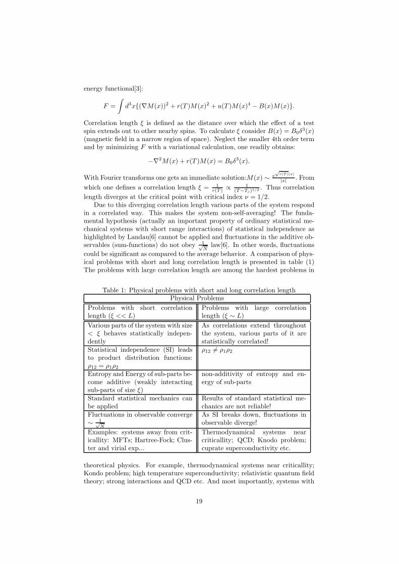
could be significant as compared to the average behavior. A comparison of phys-ical problems with short and long correlation length is presented in table (1)The problems with large correlation length are among the hardest problems in

Table 1: Physical problems with short and long correlation lengthPhysical Problems

Problems with short correlationlength (ξ << L)

Problems with large correlationlength (ξ ∼ L)

Various parts of the system with size< ξ behaves statistically indepen-dently

As correlations extend throughoutthe system, various parts of it arestatistically correlated!

Statistical independence (SI) leadsto product distribution functions:ρ12 = ρ1ρ2

ρ12 6= ρ1ρ2

Entropy and Energy of sub-parts be-come additive (weakly interactingsub-parts of size ξ)

non-additivity of entropy and en-ergy of sub-parts

Standard statistical mechanics canbe applied

Results of standard statistical me-chanics are not reliable!

Fluctuations in observable converge∼ 1√

N

As SI breaks down, fluctuations inobservable diverge!

Examples: systems away from crit-icallity: MFTs; Hartree-Fock; Clus-ter and virial exp...

Thermodynamical systems nearcriticallity; QCD; Knodo problem;cuprate superconductivity etc.

theoretical physics. For example, thermodynamical systems near criticallity;Kondo problem; high temperature superconductivity; relativistic quantum fieldtheory; strong interactions and QCD etc. And most importantly, systems with

19

Kadanoff’s construction2−D Ising Model

16 original spins

spins are well correlated on l<< ξ

4 effective spins

effective lattice

Figure 16: Kadanoff’s Block spin renormalization idea

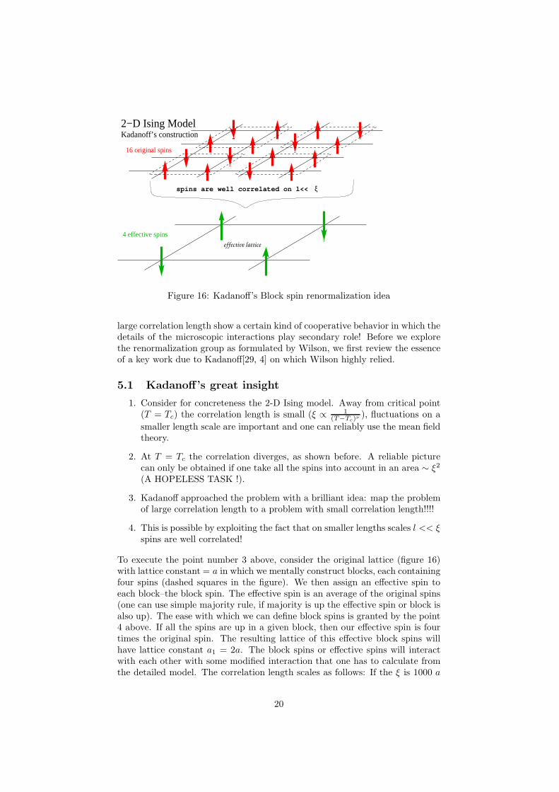
large correlation length show a certain kind of cooperative behavior in which thedetails of the microscopic interactions play secondary role! Before we explorethe renormalization group as formulated by Wilson, we first review the essenceof a key work due to Kadanoff[29, 4] on which Wilson highly relied.

5.1 Kadanoff’s great insight

1. Consider for concreteness the 2-D Ising model. Away from critical point(T = Tc) the correlation length is small (ξ ∝ 1

(T−Tc)ν), fluctuations on a

smaller length scale are important and one can reliably use the mean fieldtheory.

2. At T = Tc the correlation diverges, as shown before. A reliable picturecan only be obtained if one take all the spins into account in an area ∼ ξ2

(A HOPELESS TASK !).

3. Kadanoff approached the problem with a brilliant idea: map the problemof large correlation length to a problem with small correlation length!!!!

4. This is possible by exploiting the fact that on smaller lengths scales l << ξspins are well correlated!

To execute the point number 3 above, consider the original lattice (figure 16)with lattice constant = a in which we mentally construct blocks, each containingfour spins (dashed squares in the figure). We then assign an effective spin toeach block–the block spin. The effective spin is an average of the original spins(one can use simple majority rule, if majority is up the effective spin or block isalso up). The ease with which we can define block spins is granted by the point4 above. If all the spins are up in a given block, then our effective spin is fourtimes the original spin. The resulting lattice of this effective block spins willhave lattice constant a1 = 2a. The block spins or effective spins will interactwith each other with some modified interaction that one has to calculate fromthe detailed model. The correlation length scales as follows: If the ξ is 1000 a

20

(in the original lattice), then it will be 500 a1 (in the scaled lattice).Thus the problem with ξ = 1000 is reduced to the problem with ξ = 500!

Repetition of this procedure ultimately leads to ξ ∼ 1 (for a finite system). Butfor a system in thermodynamical limit (system of infinite extent) one can exploitthe following fundamental fact: “ξ diverges at the critical point” This funda-mental fact in an infinite system leads to a very curious behavior of system’scouplings. They tend towards a fixed point as explained below:

Let the Hamiltonian of un-scaled system be H =∑

n,iK0snsn+i. HereK0 is near neighbor interaction in the un-scaled lattice. After first scaling, let

K0 → Keff1 and sn → s

(1)n (i.e., block spins s

(1)n interact with effective coupling

Keff1 ). Thus after first scaling:

∑

n,i

K0snsn+i →∑

n,i

Keff1 s(1)n s

(1)n+i.

After m repetitions:

H(m)effective =

∑

n,i

Keffm s(m)

n s(m)n+i.

The correlation length behaves as follows:After first scaling ξ(1)(Keff

1 ) = 12ξ(K0) (If the ξ is 1000 a (in the origi-

nal lattice), then it will be 500 a1 (in the scaled lattice)). After m-scalings: ξ(m)(Keff

m ) = 12m ξ(K0). Now the fundamental assumption that goes in

Kadanoff treatment is this: The scaling does not change the physics of theproblem, namely, ξ(m)(Keff

m ) diverges as Keffm → Kc as the original correla-

tion length ξ(K0) does at Kc (Kc = JkBTc

). If one knows the functional form

Keffm = f(Keff

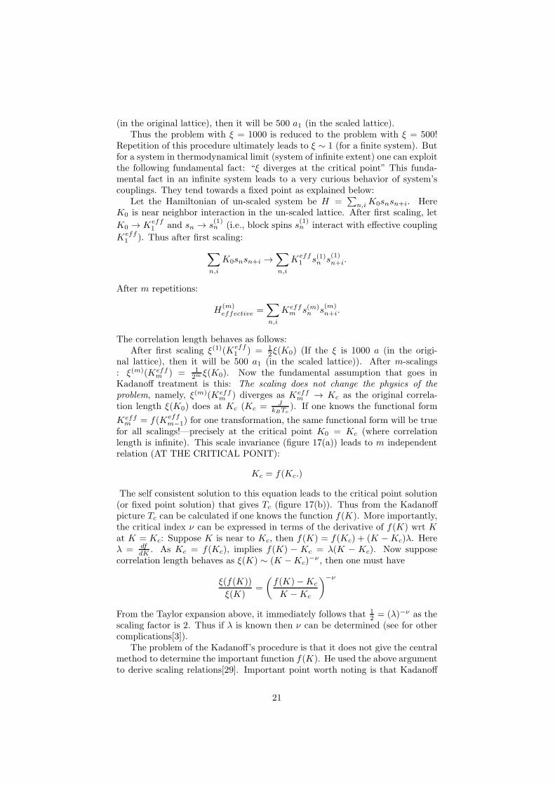
m−1) for one transformation, the same functional form will be truefor all scalings!—precisely at the critical point K0 = Kc (where correlationlength is infinite). This scale invariance (figure 17(a)) leads to m independentrelation (AT THE CRITICAL PONIT):

Kc = f(Kc.)

The self consistent solution to this equation leads to the critical point solution(or fixed point solution) that gives Tc (figure 17(b)). Thus from the Kadanoffpicture Tc can be calculated if one knows the function f(K). More importantly,the critical index ν can be expressed in terms of the derivative of f(K) wrt Kat K = Kc: Suppose K is near to Kc, then f(K) = f(Kc) + (K −Kc)λ. Hereλ = df

dK . As Kc = f(Kc), implies f(K) − Kc = λ(K − Kc). Now supposecorrelation length behaves as ξ(K) ∼ (K −Kc)

−ν , then one must have

ξ(f(K))

ξ(K)=

(f(K)−Kc

K −Kc

)−ν

From the Taylor expansion above, it immediately follows that 12 = (λ)−ν as the

scaling factor is 2. Thus if λ is known then ν can be determined (see for othercomplications[3]).

The problem of the Kadanoff’s procedure is that it does not give the centralmethod to determine the important function f(K). He used the above argumentto derive scaling relations[29]. Important point worth noting is that Kadanoff

21

Scale Invariance fixed point

K

f(K)

f(K)

K

K

K co

Figure 17: (a) Scale invariance: same kind of structure re-appears at all lengthscales when correlation length diverges (if one magnifies any part of the system,then it is not possible to notice the difference between the magnified part andthe original system). (b) Fixed points: self-consistent solution of K = f(K).

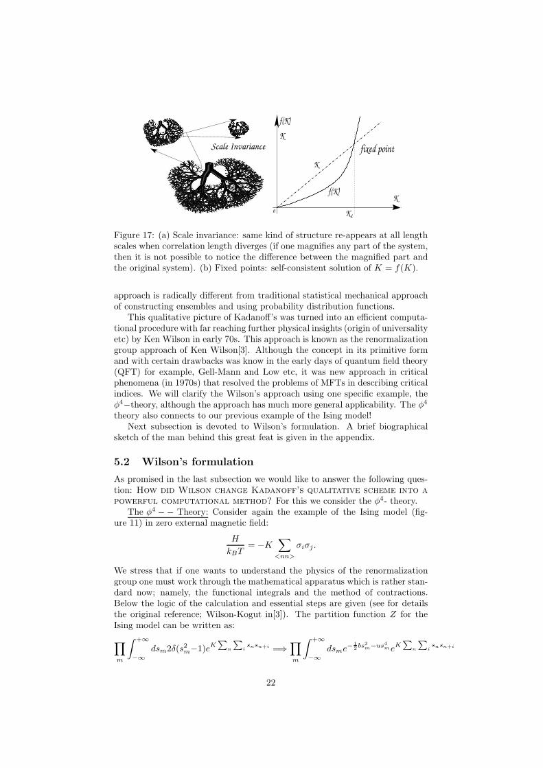
approach is radically different from traditional statistical mechanical approachof constructing ensembles and using probability distribution functions.

This qualitative picture of Kadanoff’s was turned into an efficient computa-tional procedure with far reaching further physical insights (origin of universalityetc) by Ken Wilson in early 70s. This approach is known as the renormalizationgroup approach of Ken Wilson[3]. Although the concept in its primitive formand with certain drawbacks was know in the early days of quantum field theory(QFT) for example, Gell-Mann and Low etc, it was new approach in criticalphenomena (in 1970s) that resolved the problems of MFTs in describing criticalindices. We will clarify the Wilson’s approach using one specific example, theφ4−theory, although the approach has much more general applicability. The φ4

theory also connects to our previous example of the Ising model!Next subsection is devoted to Wilson’s formulation. A brief biographical

sketch of the man behind this great feat is given in the appendix.

5.2 Wilson’s formulation

As promised in the last subsection we would like to answer the following ques-tion: How did Wilson change Kadanoff’s qualitative scheme into a

powerful computational method? For this we consider the φ4- theory.The φ4 −− Theory: Consider again the example of the Ising model (fig-

ure 11) in zero external magnetic field:

H

kBT= −K

∑

<nn>

σiσj .

We stress that if one wants to understand the physics of the renormalizationgroup one must work through the mathematical apparatus which is rather stan-dard now; namely, the functional integrals and the method of contractions.Below the logic of the calculation and essential steps are given (see for detailsthe original reference; Wilson-Kogut in[3]). The partition function Z for theIsing model can be written as:

∏

m

∫ +∞

−∞dsm2δ(s2m−1)eK

∑

n

∑

isnsn+i =⇒

∏

m

∫ +∞

−∞dsme

− 12 bs

2m−us4meK

∑

n

∑

isnsn+i

22

Sm+1 −1 +1 −1

Sm

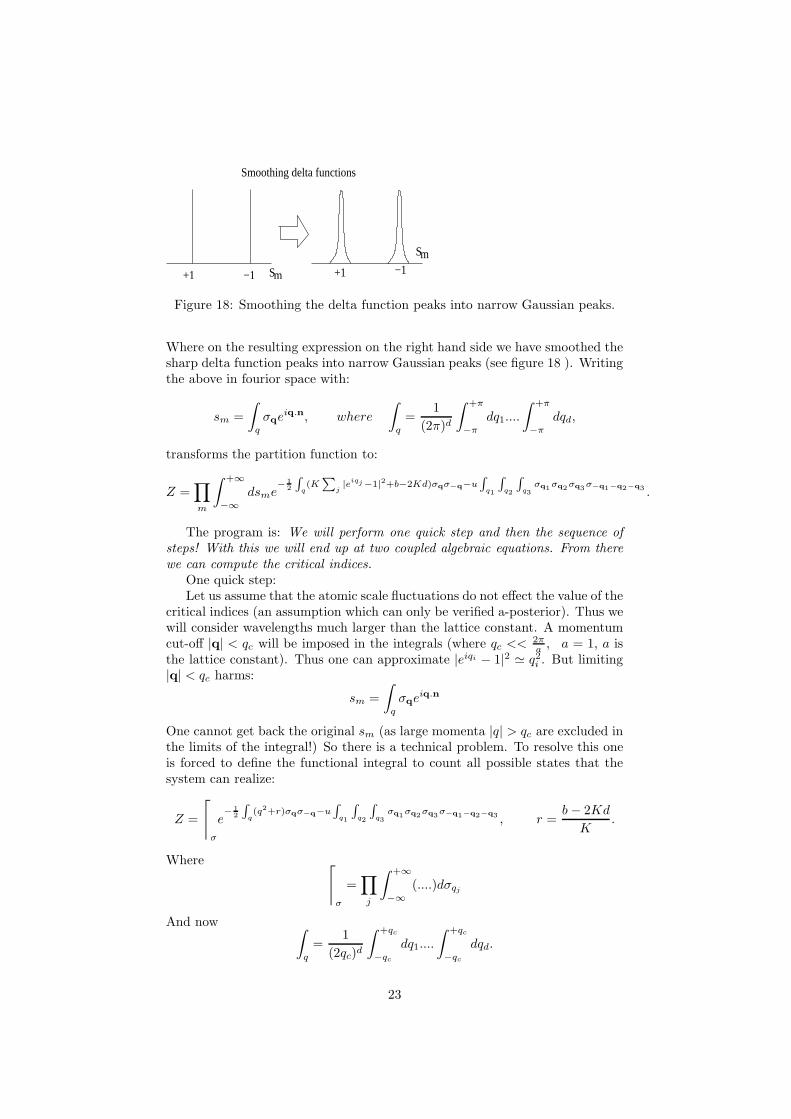
Smoothing delta functions

Figure 18: Smoothing the delta function peaks into narrow Gaussian peaks.

Where on the resulting expression on the right hand side we have smoothed thesharp delta function peaks into narrow Gaussian peaks (see figure 18 ). Writingthe above in fourior space with:

sm =

∫

q

σqeiq.n, where

∫

q

=1

(2π)d

∫ +π

−π

dq1....

∫ +π

−π

dqd,

transforms the partition function to:

Z =∏

m

∫ +∞

−∞dsme

− 12

∫

q(K∑

j|eiqj−1|2+b−2Kd)σqσ−q−u

∫

q1

∫

q2

∫

q3σq1σq2σq3σ−q1−q2−q3 .

The program is: We will perform one quick step and then the sequence ofsteps! With this we will end up at two coupled algebraic equations. From therewe can compute the critical indices.

One quick step:Let us assume that the atomic scale fluctuations do not effect the value of the

critical indices (an assumption which can only be verified a-posterior). Thus wewill consider wavelengths much larger than the lattice constant. A momentumcut-off |q| < qc will be imposed in the integrals (where qc <<

2πa , a = 1, a is

the lattice constant). Thus one can approximate |eiqi − 1|2 ≃ q2i . But limiting|q| < qc harms:

sm =

∫

q

σqeiq.n

One cannot get back the original sm (as large momenta |q| > qc are excluded inthe limits of the integral!) So there is a technical problem. To resolve this oneis forced to define the functional integral to count all possible states that thesystem can realize:

Z =

⌈

σ

e− 1

2

∫

q(q2+r)σqσ−q−u

∫

q1

∫

q2

∫

q3σq1σq2σq3σ−q1−q2−q3 , r =

b − 2Kd

K.

Where ⌈

σ

=∏

j

∫ +∞

−∞(....)dσqj

And now ∫

q

=1

(2qc)d

∫ +qc

−qc

dq1....

∫ +qc

−qc

dqd.

23

This is one typical example of defining an Effective Field Theory (EFT)! Our aimis to execute Kadanoff’s idea of “thinning out the degrees-of-freedom”. Here weare doing in momentum space (instead in real space as was done in the previousexample of the last subsection). Higher momentum states will be integratedout iteratively. The logic of the procedure is given below. The fundamentalimportance of Wilson’s iterative procedure (the renormalization group) is thatwe will get the pivotal function f(K) of the previous example. From that it ispossible to get the critical point and all the critical indices etc.

The Procedure: Define the functional integral as: Z =

⌈

σ

eH[σ] with H [σ] =

− 12

∫

q(q2+r)σqσ−q−u

∫

q1

∫

q2

∫

q3σq1σq2σq3σ−q1−q2−q3 . This functional integral

can be written as the product of two functional integrals (as is clear from thedefinition of the functional integral above).

Z =

⌈

σ0

(⌈

σ1

eH[σ0+σ1]

)

︸ ︷︷ ︸

higher momenta integrals

Here

σq =

{σ0,q ≡ σ0 if 0 < |q| < qc

2σ1,q ≡ σ1 if qc

2 < |q| < qc

We want to integrate out σ1s (the higher momentum shell). Also rename variousparts of the Hamiltonian as:

H [σ] = −1

2

∫

q

(q2 + r)σqσ−q

︸ ︷︷ ︸

HF [σ]

+−u

∫

q1

∫

q2

∫

q3

σq1σq2σq3σ−q1−q2−q3

︸ ︷︷ ︸

HI [σ]

.

Let the integration of higher momenta states yields:

eH′[σ′] = eHF [σ0]

⌈

σ1

eHF [σ1]+HI [σ0+σ1].

Here we define σ′ ≡ σ′q′ = 1

ζσ0,q (i.e., σ′ and q′ are rescaled variables with

0 < |q′| < qc and 0 < |q| < qc2 ). HF [σ0] can be written in terms of scaled

variables trivially as:

−1

2

∫

0<|q|< qc2

(q2 + r)σqσ−q =⇒ −1

2(ζ22−d−2)

∫

0<|q′|<qc

(q′2+ 4r)

︸ ︷︷ ︸

notice!

σ′q′σ′

−q′ .

This trivial scaling cannot be done on the interaction term (due to coupling ofmomenta). One must use perturbation theory and express:

eHI [σ] ≃ 1−×+1

2(×)(×)− ...

Where × ≡ −HI [σ]. In this series expansion inside the functional integral onewill encounter terms like:

I(q1,q2, ....qk) =

⌈

σ1

σ1,q1σ1,q2 .........σ1,qkeHF [σ1] ∝ {σ1,q1σ1,q2σ1,q3σ1,q4 ......+ ....all combinations...} .

24

un+1 = nuun+1

u* unu0 u (T )0

r (T )0c c

u r* *

u

r

fixed pt

direction of iterations

1

2

3 Starting pts.

D

(a) (b)

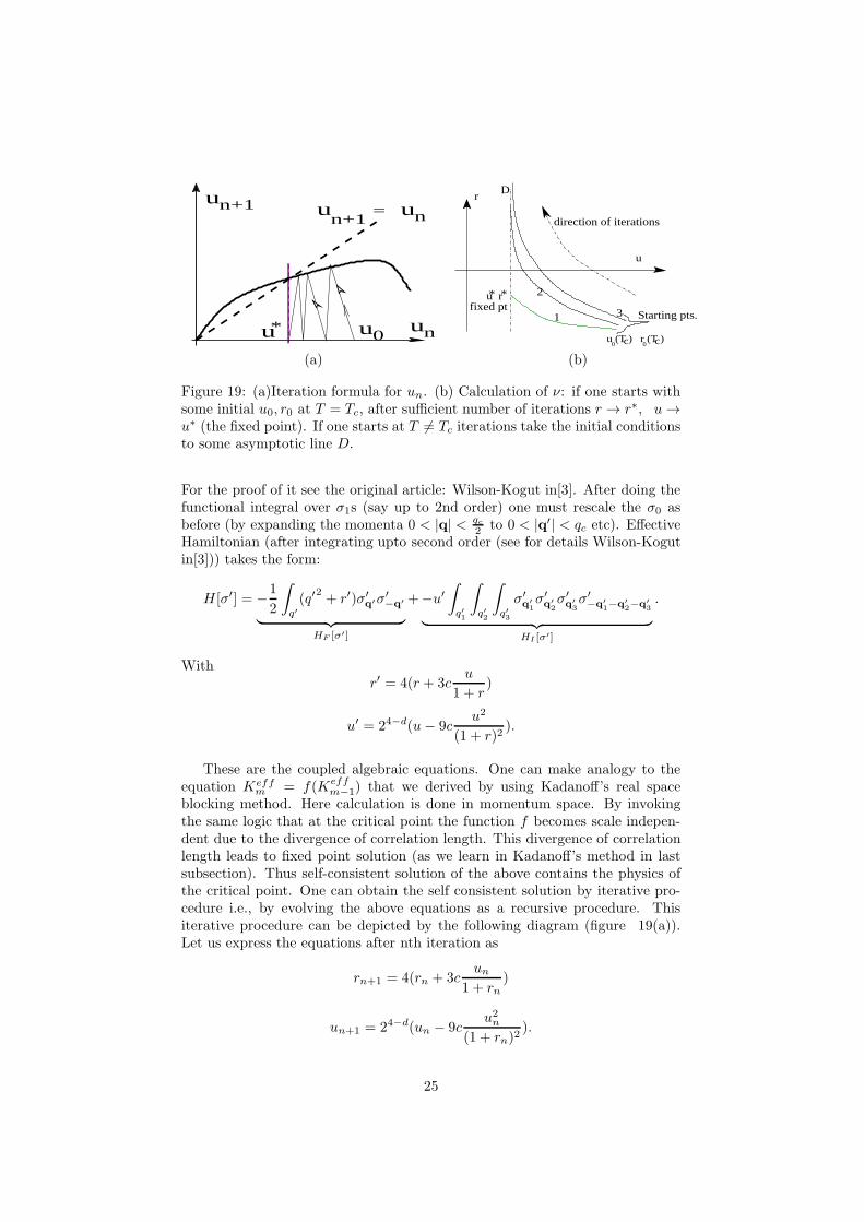
Figure 19: (a)Iteration formula for un. (b) Calculation of ν: if one starts withsome initial u0, r0 at T = Tc, after sufficient number of iterations r → r∗, u→u∗ (the fixed point). If one starts at T 6= Tc iterations take the initial conditionsto some asymptotic line D.

For the proof of it see the original article: Wilson-Kogut in[3]. After doing thefunctional integral over σ1s (say up to 2nd order) one must rescale the σ0 asbefore (by expanding the momenta 0 < |q| < qc

2 to 0 < |q′| < qc etc). EffectiveHamiltonian (after integrating upto second order (see for details Wilson-Kogutin[3])) takes the form:

H [σ′] = −1

2

∫

q′(q′

2+ r′)σ′

q′σ′−q′

︸ ︷︷ ︸

HF [σ′]

+−u′∫

q′1

∫

q′2

∫

q′3

σ′q′1σ′q′2σ′q′3σ′−q

′1−q

′2−q

′3

︸ ︷︷ ︸

HI [σ′]

.

Withr′ = 4(r + 3c

u

1 + r)

u′ = 24−d(u− 9cu2

(1 + r)2).

These are the coupled algebraic equations. One can make analogy to theequation Keff

m = f(Keffm−1) that we derived by using Kadanoff’s real space

blocking method. Here calculation is done in momentum space. By invokingthe same logic that at the critical point the function f becomes scale indepen-dent due to the divergence of correlation length. This divergence of correlationlength leads to fixed point solution (as we learn in Kadanoff’s method in lastsubsection). Thus self-consistent solution of the above contains the physics ofthe critical point. One can obtain the self consistent solution by iterative pro-cedure i.e., by evolving the above equations as a recursive procedure. Thisiterative procedure can be depicted by the following diagram (figure 19(a)).Let us express the equations after nth iteration as

rn+1 = 4(rn + 3cun

1 + rn)

un+1 = 24−d(un − 9cu2n

(1 + rn)2).

25

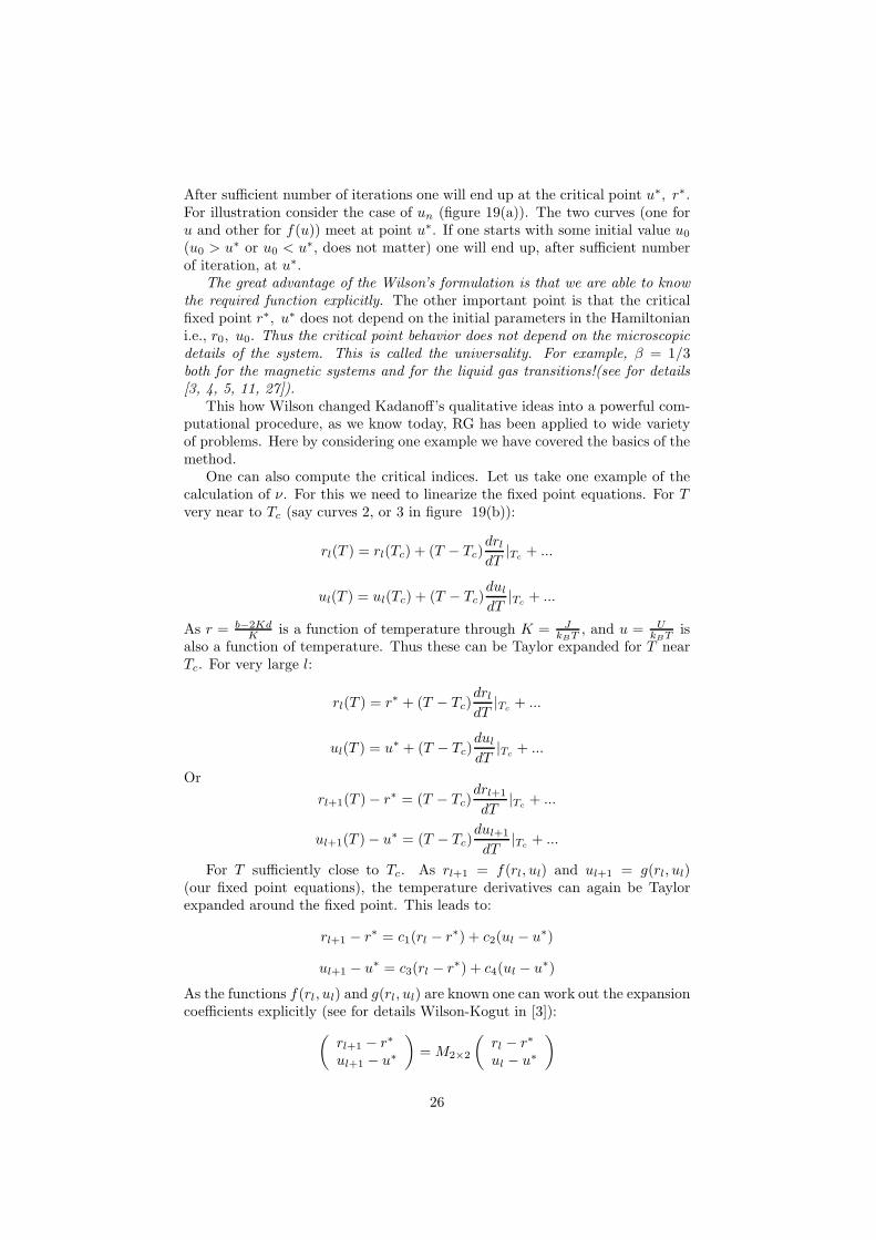
After sufficient number of iterations one will end up at the critical point u∗, r∗.For illustration consider the case of un (figure 19(a)). The two curves (one foru and other for f(u)) meet at point u∗. If one starts with some initial value u0(u0 > u∗ or u0 < u∗, does not matter) one will end up, after sufficient numberof iteration, at u∗.

The great advantage of the Wilson’s formulation is that we are able to knowthe required function explicitly. The other important point is that the criticalfixed point r∗, u∗ does not depend on the initial parameters in the Hamiltoniani.e., r0, u0. Thus the critical point behavior does not depend on the microscopicdetails of the system. This is called the universality. For example, β = 1/3both for the magnetic systems and for the liquid gas transitions!(see for details[3, 4, 5, 11, 27]).

This how Wilson changed Kadanoff’s qualitative ideas into a powerful com-putational procedure, as we know today, RG has been applied to wide varietyof problems. Here by considering one example we have covered the basics of themethod.

One can also compute the critical indices. Let us take one example of thecalculation of ν. For this we need to linearize the fixed point equations. For Tvery near to Tc (say curves 2, or 3 in figure 19(b)):

rl(T ) = rl(Tc) + (T − Tc)drldT

|Tc + ...

ul(T ) = ul(Tc) + (T − Tc)duldT

|Tc + ...

As r = b−2KdK is a function of temperature through K = J

kBT , and u = UkBT is

also a function of temperature. Thus these can be Taylor expanded for T nearTc. For very large l:

rl(T ) = r∗ + (T − Tc)drldT

|Tc + ...

ul(T ) = u∗ + (T − Tc)duldT

|Tc + ...

Or

rl+1(T )− r∗ = (T − Tc)drl+1

dT|Tc + ...

ul+1(T )− u∗ = (T − Tc)dul+1

dT|Tc + ...

For T sufficiently close to Tc. As rl+1 = f(rl, ul) and ul+1 = g(rl, ul)(our fixed point equations), the temperature derivatives can again be Taylorexpanded around the fixed point. This leads to:

rl+1 − r∗ = c1(rl − r∗) + c2(ul − u∗)

ul+1 − u∗ = c3(rl − r∗) + c4(ul − u∗)

As the functions f(rl, ul) and g(rl, ul) are known one can work out the expansioncoefficients explicitly (see for details Wilson-Kogut in [3]):

(rl+1 − r∗

ul+1 − u∗

)

=M2×2

(rl − r∗

ul − u∗

)

26

By iterating n−times:

(rl+n − r∗

ul+n − u∗

)

= (M2×2)n

(rl − r∗

ul − u∗

)

The purpose of iterating n-times is that the matrixMn is completely dominatedby the largest eigenvalue λn (λ = 4 for u = 0 case). One can find eigensystemof the above matrix and finally (as the largest eigenvalue dominates!):

rl+n − r∗ ≃ λn1w11cl(T − Tc).

here λ1 is the largest eigen value, w11 is the corresponding eigenvector, and cl isa constant (see for details Wilson-Kogut in[3]). And a similar expression holdsfor the ul. One observe that:

rl+n+1(T )− r∗ at (T − Tc =τ

λ1) = rl+n(T )− r∗ at T − Tc = τ

Thus the correlation length:

ξ(rl+n+1, ul+n+1)∣∣T=Tc+τ/λ1

= ξ(rl+n, ul+n)∣∣T=Tc+τ

.

Now

1

2l+n+1ξ(Tc + τ/λ1) =

1

2l+nξ(Tc + τ), as ξ(rl+n, ul+n) =

1

2l+nξ(r0, u0).

If correlation length scales as:

ξ(Tc + τ) ∝ τ−ν

Then from above:

(τ

λ1)−ν = 2τ−ν =⇒ ν =

ln2

lnλ1.

If u = 0 (simple Gaussian model), then λ1 = 4 which leads to ν = 0.5 (the MFTresult). With explicit calculation of λ1 for u 6= 0 (see for details Wilson-Kogutin[3]), ν comes out to be:

ν ≃ 0.58

This is very close to the experimentally observed value ν = 0.6 (in MFT it is0.5!!!!). Similarly other critical indices can be calculated and are quite close towhat is observed experimentally[11, 27].

6 Why do MFTs fail and how does RGT rectifythat?

Thus, by exploiting scale invariance at the critical point and by finding the crit-ical point from fixed point equations by iterative procedure one is able to calcu-lated correct values of critical indices. The important point that goes implicit inthe above statement is that iterative procedure is not only a mathematical de-vice to reach to the fixed point but also at each step of iteration one is averagingover smaller length scale (or higher momentum scale) fluctuations and with thisappropriate averaging over increasingly longer length scales one is able calculate

27

the correct values of critical indices. With this sophistication of renormalizationgroup method we immediately see the drawback of MFTs. In MFTs we do anabrupt step in dealing with the fluctuations: 〈σ〉 = tanh(h + Tc

T 〈σ〉) i.e., weaverage out only the smaller length scale (of the order of lattice constant) fluc-tuations (in calculating the effective field seen by the test spin). Near the criticalpoint just below the critical temperature, ensemble averages over smaller lengthscales (of the order of lattice constant) lead to zero value of the order parameter(here mean magnetization). Only when one averages over a large length scale(of the order of correlation length) can one see some tiny magnetization just be-low criticality. Thus our assumption of tiny mean magnetization over a smallerlength scale (of the order of lattice constant) in MFT breaks down! And MFTpredicts wrong values of critical indices( see also[7]).

7 Appendix: K. G. Wilson–a short biographicalsketch

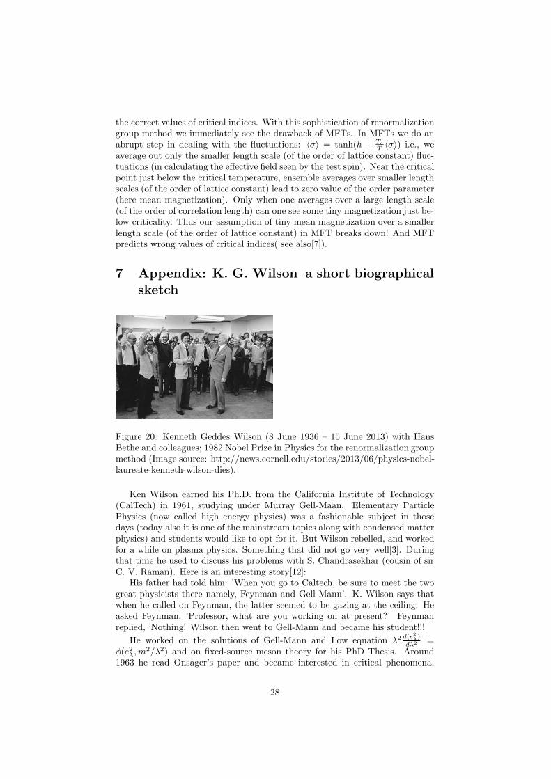
Figure 20: Kenneth Geddes Wilson (8 June 1936 – 15 June 2013) with HansBethe and colleagues; 1982 Nobel Prize in Physics for the renormalization groupmethod (Image source: http://news.cornell.edu/stories/2013/06/physics-nobel-laureate-kenneth-wilson-dies).

Ken Wilson earned his Ph.D. from the California Institute of Technology(CalTech) in 1961, studying under Murray Gell-Maan. Elementary ParticlePhysics (now called high energy physics) was a fashionable subject in thosedays (today also it is one of the mainstream topics along with condensed matterphysics) and students would like to opt for it. But Wilson rebelled, and workedfor a while on plasma physics. Something that did not go very well[3]. Duringthat time he used to discuss his problems with S. Chandrasekhar (cousin of sirC. V. Raman). Here is an interesting story[12]:

His father had told him: ’When you go to Caltech, be sure to meet the twogreat physicists there namely, Feynman and Gell-Mann’. K. Wilson says thatwhen he called on Feynman, the latter seemed to be gazing at the ceiling. Heasked Feynman, ’Professor, what are you working on at present?’ Feynmanreplied, ’Nothing! Wilson then went to Gell-Mann and became his student!!!

He worked on the solutions of Gell-Mann and Low equation λ2d(e2λ)dλ2 =

φ(e2λ,m2/λ2) and on fixed-source meson theory for his PhD Thesis. Around

1963 he read Onsager’s paper and became interested in critical phenomena,

28

and after that studying other works on critical phenomena he developed therenormalization group theory, using tricks and techniques that he had learnt inparticle physics.

References

[1] van der Waals, Nobel Lecture (Nobel prize 1910), Physics, 1901, ElsevierPub. Company, Amsterdam (1967).

[2] L. D. Landau, Phys. Zurn. Sowjetunion 26, 11 (1937) [see collected papersof Lev Landau; D ter Haar, Vol II, Pergamon Press, Oxford, 1969].

[3] K. G. Wilson, Rev. Mod. Phys. 55, 583 (1983); K. G. Wilson and J.Kogut, Phys. Rep. 12, 75 (1974).

[4] Leo Kadanoff, arXiv: 1002.2985v1 (2010); Leo Kadanoff, J. Stat. Phys.137, 777 (2009).

[5] K. G. Wilson, Scientific American , 158 (1979).

[6] L. D. Landau and E. M. Lifschitz, Statistical Physics, Vol. 6, PergamonPress, U.K.(1980).

[7] Navinder Singh, accompanying paper, arXiv:..... (2014).

[8] K. G. Wilson, Rev. Mod. Phys. 47, 773 (1975).

[9] R. Shankar, Rev. Mod. Phys. 66, 129 (1994).

[10] S. R. White, Phys. Rev. Lett. 69, 2863 (1992).

[11] J. Zinn-Justin, Quantum field theory and critical phenomena, Oxford,Clarendon Press (2002); N. Goldenfeld, Lectures on Phase transitions andthe renormalization group, Addison-Wesley (1992).

[12] G. Venkataraman, The many phases of matter, Universities Press, India(1997).

[13] A. Leggett, Quantum liquids: Bose condensation and cooper pairing incondensed-matter systems, OUP, Oxford (2006).

[14] L. D. Landau and E. M. Lifschitz, Statistical Physics, Part 2, Vol. 9,Pergamon Press, U. K.(1980).

[15] J. Bardeen, L. Cooper, R. Schrieffer, Phys. Rev. 108, 1175 (1957).

[16] P. W. Anderson and P. Morel, Phys. Rev. 123, 1911 (1963).

[17] D. J. Scalapino, Rev. Mod. Phys. 84, 1383 (2012); P. W. Anderson, Int.J. Mod. Phys. B 25, 1 (2011).

[18] Charles Kittel, Introduction to solid state physics, 6th Ed. John Wiley andsons (1986).

[19] J. Hubbard, Phys. Rev. B 19, 2626 (1979).

29

[20] T. W. B. Kibble, Phys. Rep. 67, 183 (1980).

[21] P. W. Higgs, Phys. Lett. 12, 132 (1964).

[22] A. B. Pippard, Elements of classical thermodynamics, CUP, U.K. (1966).

[23] G. Gallavotti, W. L. Reiter, J. Yngvason, Boltzmann Legacy, EuropeanMath. Soc. (2008); Navinder Singh, Mod. Phys. Lett. B 27, 1330003(2013).

[24] A. Scott, J. of Consciousness Studies, 11, 51 (2004); Eric R. Kandel,In search of memory: the emergence of a new science of mind, Norton(2007); P. W. Anderson, Science, 177, 4047 (1972); R. B. Laughlin andDavid Pines, PNAS 97, 28 (2000).

[25] P. W. Atkins and J. de Paula, Physical Chemistry, OUP, Oxford (2002).

[26] S. N. Isakov, Comm. Math. Phys. 95, 427 (1984).

[27] Leo Kadanoff, Statistical Physics–statics, dynamics and renormalization,WS (2000).

[28] K. Huang, Statistical Mechanics, Wiley, Canada (1987).

[29] L. P. Kadanoff, Physics, 2, 263 (1965).

30