Semiempirical modeling of abiotic and biotic factorscontrolling ecosystem respiration across eddy covariancesitesM I R C O M I G L I AVA C C A *w , M A R K U S R E I C H S T E I N w , A N D R E W D . R I C H A R D S O N z,R O B E R T O C O L O M B O *, M A R K A . S U T T O N § , G I T T A L A S S L O P w , E N R I C O T O M E L L E R I w ,

G E O R G W O H L F A H R T } , N U N O C A R VA L H A I S kw , A L E S S A N D R O C E S C AT T I **,

M I G U E L D . M A H E C H A w w w , L E O N A R D O M O N T A G N A N I zz, § § , D A R I O PA PA L E } } ,

S O N K E Z A E H L E kk, A L T A F A R A I N ***, A L M U T A R N E T H w w w , T . A N D R E W B L A C K zzz,ARNAUD CARRARA§§§, SABINA DORE}}} , DAMIANO GIANELLEkkk, CAROLE HELFTER§ ,

D AV I D H O L L I N G E R ****, W E R N E R L . K U T S C H w w w w , P E T E R M . L A F L E U R zzzz,YA N N N O U V E L L O N § § § § , C O R I N N A R E B M A N N } } } } kkkk, H U M B E R T O R . D A R O C H A *****,

MIRCO RODEGHIEROkkk, OL IVIE R ROUPSARD§§§§wwwww , MARIA-TERESA SE BASTIAzzzzz§ § § § § ,

G U E N T H E R S E U F E R T **, J E A N - F R A N C O I S E S O U S S A N A } } } } } and

M I C H I E L K . VA N D E R M O L E N kkkkk*Remote Sensing of Environmental Dynamics Laboratory, DISAT, University of Milano-Bicocca, P.zza della Scienza 1, 20126,

Milano, Italy, wModel Data Integration Group, Max Planck Institute for Biogeochemistry, Postfach 10 01 64, 07701 Jena, Germany,

zDepartment of Organismic and Evolutionary Biology, Harvard University, Cambridge, MA 02138, USA, §Centre for Ecology and

Hydrology, Edinburgh Research Station, Bush Estate, Penicuik, Midlothian, Scotland EH26 0QB, UK, }Institut fur Okologie,

Universitat Innsbruck, 6020 Innsbruck, Austria, kFaculdade de Ciencias e Tecnologia, FCT, Universidade Nova de Lisboa, 2829-516

Caparica, Portugal, **European Commission, DG-JRC, Institute for Environment and Sustainability, Climate Change Unit, Via Enrico

Fermi 2749, T.P. 050, 21027 Ispra (VA), Italy, wwDepartment of Environmental Sciences, Swiss Federal Institute of Technology-ETH

Zurich, 8092 Zurich, Switzerland, zzProvincia Autonoma di Bolzano, Agenzia per l’Ambiente; Servizi Forestali, 39100 Italy, §§Free

University of Bolzano/Bozen, Faculty of Science and Technology, Piazza Universita, 5, 39100 Bozen-Bolzano, Italy, }}DISAFRI,

University of Tuscia, via C. de Lellis, 01100 Viterbo Italy, kkDepartment for Biogeochemical System, Max Planck Institute for

Biogeochemistry, Postfach 10 01 64, 07701 Jena, Germany, ***McMaster University, School of Geography & Earth Sciences, 1280 Main

Street West, Hamilton, ON, Canada L8S 4K1, wwwDepartment of Physical Geography and Ecosystems Analysis, Lund University,

Solvegatan 12, SE-223 62 Lund, Sweden, zzzFaculty of Land and Food Systems, University of British Columbia, Vancouver, BC,

V6T 1Z4 Canada, §§§Fundacion Centro de Estudios Ambientales del Mediterraneo (CEAM), Program of Air Pollutants Effects,

Calle Charles H. Darwin, 14, 46980 Paterna, Spain, }}}Department of Biological Sciences and Merriam-Powell Center for

Environmental Research, Northern Arizona University, Flagstaff, AZ 86011, USA, kkkIASMA Research and Innovation Centre,

Fondazione E. Mach, Environment and Natural Resources Area, San Michele all’Adige, I-38040 Trento, Italy, ****USDA Forest Service,

NE Research Station, Durham, NH 03824, USA, wwwwJohann Heinrich von Thunen Institut (vTI), Institut fur Agrarrelevante

Klimaforschung, 38116 Braunschweig, Germany, zzzzDepartment of Geography, Trent University, Peterborough, ON, Canada K 9J 7B8,

§§§§CIRAD, Persyst, UPR80, TA10/D, 34398 Montpellier Cedex 5, France, }}}}Department of Micrometeorology, University of

Bayreuth, Postfach 10 01 64, 07701 Bayreuth, Germany, kkkkMax Planck Institute for Biogeochemistry, Jena, Germany,*****Departamento de Ciencias Atmosfericas/IAG/Universidade de Sao Paulo, Rua do Matao, 1226 Cidade Universitaria, Sao Paulo, SP,

Brazil, wwwwwCATIE, Centro Agronomico Tropical de Investigacion y Ensenanza, Turrialba 7170, Costa Rica, zzzzzLaboratory of Plant

Ecology and Botany, Forest Technology Centre of Catalonia, 25280 Solsona, Spain, §§§§§Agronomical Engineering School, University of

Lleida, E-25198 Lleida, Spain, }}}}}INRA, Grassland Ecosyst Res UR874, F-63100 Clermont Ferrand, France, kkkkkDepartment of

Hydrology and Geo-Environmental Sciences, VU-University, de Boeleaan 1085, 1081 HVAmsterdam, The Netherlands

Abstract

In this study we examined ecosystem respiration (RECO) data from 104 sites belonging to FLUXNET, the global

network of eddy covariance flux measurements. The goal was to identify the main factors involved in the variability of

RECO: temporally and between sites as affected by climate, vegetation structure and plant functional type (PFT)

(evergreen needleleaf, grasslands, etc.). We demonstrated that a model using only climate drivers as predictors of

RECO failed to describe part of the temporal variability in the data and that the dependency on gross primary

production (GPP) needed to be included as an additional driver of RECO. The maximum seasonal leaf area index

Correspondence: Mirco Migliavacca, tel. 1 39 026 448 2848, fax 1 39 026 448 2895, e-mail: m.migliavacca1@campus.unimib.it

Global Change Biology (2011) 17, 390–409, doi: 10.1111/j.1365-2486.2010.02243.x

390 r 2010 Blackwell Publishing Ltd

(LAIMAX) had an additional effect that explained the spatial variability of reference respiration (the respiration at

reference temperature Tref 5 15 1C, without stimulation introduced by photosynthetic activity and without water

limitations), with a statistically significant linear relationship (r2 5 0.52, Po0.001, n 5 104) even within each PFT.

Besides LAIMAX, we found that reference respiration may be explained partially by total soil carbon content (SoilC).

For undisturbed temperate and boreal forests a negative control of total nitrogen deposition (Ndepo) on reference

respiration was also identified. We developed a new semiempirical model incorporating abiotic factors (climate),

recent productivity (daily GPP), general site productivity and canopy structure (LAIMAX) which performed well in

predicting the spatio-temporal variability of RECO, explaining 470% of the variance for most vegetation types.

Exceptions include tropical and Mediterranean broadleaf forests and deciduous broadleaf forests. Part of the

variability in respiration that could not be described by our model may be attributed to a series of factors, including

phenology in deciduous broadleaf forests and management practices in grasslands and croplands.

Keywords: ecosystem respiration, eddy covariance, FLUXNET, inverse modeling, leaf area index, productivity

Received 7 January 2010 and accepted 22 February 2010

Introduction

Respiration of terrestrial ecosystems (RECO) is one of the

major fluxes in the global carbon cycle and its responses

to environmental change are important in understand-

ing climate–carbon cycle interactions (e.g. Houghton

et al., 1998; Cox et al., 2000). It has been hypothesized

that relatively small climatic changes may impact re-

spiration with the effect of rivaling the annual fossil fuel

loading of atmospheric CO2 (Jenkinson et al., 1991;

Raich & Schlesinger, 1992).

Recently, efforts have been made to mechanistically

understand how temperature and other environmental

factors affect ecosystem and soil respiration, and var-

ious modeling approaches have been proposed (e.g.

Lloyd & Taylor, 1994; Reichstein et al., 2003a; Davidson

et al., 2006a; Reichstein & Beer, 2008). Nevertheless, the

conceptual processes and complex interactions control-

ling RECO are still incompletely understood and the

associated uncertainty continues to hamper bottom-up

scaling to larger spatial scales (e.g. regional and con-

tinental), which is one of the major challenges for

biogeochemists and climatologists.

Heterotrophic and autotrophic respiration in both

data-oriented and process-based biogeochemical mod-

els are usually described as a function of air or soil

temperature and occasionally soil water content (e.g.

Lloyd & Taylor, 1994; Thornton et al., 2002; Reichstein

et al., 2005), although the functional form of these

relationships varies from model to model. These func-

tions represent the dominant role of reaction kinetics,

possibly modulated or confounded by other environ-

mental factors such as soil water content or precipita-

tion, which some model formulations include as a

secondary effect (e.g. Carlyle & Ba Than, 1988; Reich-

stein et al., 2003a; Richardson et al., 2006).

A large number of statistical, climate-driven models

of ecosystem and soil respiration have been tested and

compared using data from individual sites (Janssens &

Pilegaard, 2003; Del Grosso et al., 2005; Richardson &

Hollinger, 2005; Savage et al., 2009), multiple sites (Falge

et al., 2001; Rodeghiero & Cescatti, 2005), and from a

wide range of models compared across different eco-

system types and measurement techniques (Richardson

et al., 2006).

Over the course of the last decades, the scientific

community has debated the role of productivity in

determining ecosystem and soil respiration. Several

authors (Valentini et al., 2000; Janssens et al., 2001;

Reichstein et al., 2003a; Curiel-Yuste et al., 2004; David-

son et al., 2006a; Bahn et al., 2008) have discussed and

clarified the role of photosynthetic activity, vegetation

productivity and their relationship to respiration.

Linking photosynthesis and respiration might be of

particular relevance when modeling RECO across

biomes or at the global scale. Empirical evidence for

the link between gross primary production (GPP) and

RECO is reported for most, if not all, ecosystems: grass-

lands (e.g. Craine et al., 1999; Hungate et al., 2002; Bahn

et al., 2008, 2009), crops (e.g. Kuzyakov & Cheng, 2001;

Moyano et al., 2007), boreal forests (Hogberg et al., 2001;

Gaumont-Guay et al., 2008) and temperate forests, both

deciduous (e.g. Curiel-Yuste et al., 2004; Liu et al., 2006)

and evergreen (e.g. Irvine et al., 2005).

Moreover, several authors have found a time lag

between productivity and respiration response. This

time lag depends on the vegetation structure: it is

related to the translocation time of assimilates from

aboveground to belowground organs through the

phloem. Although the existence of a time lag is still

under debate, it has been found to be a few hours in

grasslands and croplands and a few days in forests

(Knohl & Buchmann, 2005; Baldocchi et al., 2006; Moya-

no et al., 2008; Savage et al., 2009).

While the link between productivity and respiration

appears to be clear, to our knowledge few model

S E M I E M P I R I C A L M O D E L I N G O F E C O S Y S T E M R E S P I R A T I O N 391

r 2010 Blackwell Publishing Ltd, Global Change Biology, 17, 390–409

formulations include the effect of productivity or photo-

synthesis as a biotic driver of respiration and these

models are mainly developed for the simulation of soil

respiration using a relatively small dataset of soil re-

spiration measurements (e.g. Reichstein et al., 2003a;

Hibbard et al., 2005).

In this context, the increasing availability of ecosys-

tem carbon, water and energy flux measurements col-

lected by means of the eddy covariance technique (e.g.

Baldocchi, 2008) over different plant functional types

(PFTs) at more than 400 research sites, represents a

useful tool in understanding processes and interactions

behind carbon fluxes and ecosystem respiration. These

data serve as a backbone for bottom-up estimates of

continental carbon balance components (e.g. Papale &

Valentini, 2003; Ciais et al., 2005; Reichstein et al., 2007)

and for ecosystem model development, calibration and

validation (e.g. Baldocchi, 1997; Law et al., 2000; Reich-

stein et al., 2002, 2003b; Hanson et al., 2004; Verbeeck

et al., 2006; Owen et al., 2007). The database includes a

number of added products such as gap-filled net eco-

system exchange (NEE), GPP, RECO and meteorological

drivers (air temperature, radiation, precipitation etc.)

aggregated at different timescales (e.g. half-hourly, dai-

ly, annually) and consistent for data treatment (Reich-

stein et al., 2005; Papale et al., 2006).

In this paper we analyze RECO with a semiempirical

modeling approach at 104 different sites belonging to the

FLUXNET database with the primary objective of

synthesizing and identifying the main factors controlling

(i) the temporal variability of RECO, (ii) the between-site

variability (hereafter referred to as spatial variability).

The second objective was to provide a model that can be

used for diagnostic up-scaling of RECO from eddy covar-

iance flux sites to large spatial scales.

Specifically, the analysis and model development

followed these three steps:

(1) we developed a semiempirical RECO model site by

site (site-by-site analysis) with the aim of clarifying

if and how GPP should be included in a model for

improving the description of RECO and which fac-

tors are best suited for describing the spatial varia-

bility of reference respiration (i.e. the daily RECO at

the reference temperature without moisture limita-

tions). We performed the following two steps:

� the analysis of RECO data was conducted using a

purely climate-driven model: TP Model (Raich

et al., 2002). The accuracy of the model and the

main bias were analyzed and discussed;

� we evaluated the inclusion of biotic factors (i.e.

GPP) as drivers of RECO. A range of different

model formulations, which differ mainly in re-

gard to the functional responses of RECO to

photosynthesis, were tested to identify the best

model formulation for the daily description of

RECO at each site;

(2) we analyzed the variability of the reference respira-

tion estimated at each site with the aim of identify-

ing, among the different site characteristics, one or

more predictors of the spatial variability of this

crucial parameter. This can be extremely useful in

the application of the model at a large spatial scale;

(3) we optimized the developed model for each PFT

(PFT analysis) with the aim of generalizing the

model parameters in a way that can be useful in

diagnostic, PFT-based, up-scaling of RECO. The ac-

curacy of the model was assessed by a cross-valida-

tion technique and its main weak points were

critically evaluated and discussed.

Material and methods

Dataset

The data used in this analysis are from version 2 of the

LaThuile FLUXNET dataset (http://www.fluxdata.org), a

dataset including 253 research sites belonging to the FLUXNET

eddy covariance network (Baldocchi et al., 2001; Baldocchi,

2008). The analysis was restricted to 104 sites (cf. Table in

Appendices S1 and S2) on the basis of ancillary data avail-

ability [i.e. only sites containing at least both maximum

ecosystem leaf area index of understorey and overstorey

(LAIMAX) were selected] and of the time series length (all sites

containing at least 1 year of carbon fluxes and meteorological

data of good quality were used). Further, we analyzed only

those sites for which the relative standard error of the esti-

mates of model parameters E0 (activation energy) and refer-

ence respiration (R0) (see further sections for more details on

the meaning of parameters) were o50% and where E0 esti-

mates were within an acceptable range (0–450 K). Sites in

which the estimated parameters were unacceptable were

around 6% of the entire dataset.

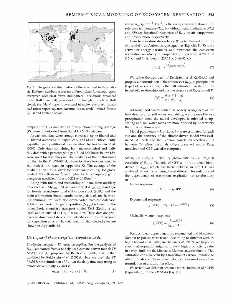
The latitude ranges from 71.321 at the Alaska Barrow site

(US-Brw) to �21.621 at the Sao Paulo Cerrado (BR-Sp1). The

climatic regions include tropical to arctic (Fig. 1).

All the main PFTs as defined by the International Geo-

sphere–Biosphere Programme (IGBP) were included in this

study: the selected sites included 28 evergreen needleleaf

forests (ENF), 17 deciduous broadleaf forests (DBF), 16 grass-

lands (GRA), 11 croplands (CRO), eight mixed forests (MF),

five savannas (SAV), nine shrublands (SHB), seven evergreen

broadleaved forests (EBF) and three wetlands (WET). Because

of the limited number of sites and their similarity, the class

SAV included both the sites classified as savanna (SAV) and

woody savannas (WSA), while the class SHB included both the

open (OSH) and closed (CSH) shrubland sites. For abbrevia-

tions and symbols refer to Appendix S3.

Daily RECO, GPP and the associated uncertainties of NEE

data, together with daily meteorological data such as mean air

392 M . M I G L I AVA C C A et al.

r 2010 Blackwell Publishing Ltd, Global Change Biology, 17, 390–409

temperature (TA) and 30-day precipitation running average

(P), were downloaded from the FLUXNET database.

At each site data were storage-corrected, spike-filtered and

u�-filtered according to Papale et al. (2006) and subsequently

gap-filled and partitioned as described by Reichstein et al.

(2005). Only days containing both meteorological and daily

flux data with a percentage of gap-filled half hours below 15%

were used for this analysis. The medians of the u� threshold

applied in the FLUXNET database for the site-years used in

the analysis are listed in Appendix S2. The average of the

median u� values is lower for short canopies (e.g. for grass-

lands 0.075 � 0.047 ms�1) and higher for tall canopies (e.g. for

evergreen needleleaf forests 0.221 � 0.115 ms�1).

Along with fluxes and meteorological data, main ancillary

data such as LAIMAX, LAI of overstorey (LAIMAX,o), stand age

for forests (StandAge), total soil carbon stock (SoilC) and the

main information about disturbance (e.g. date of cuts, harvest-

ing, thinning, fire) were also downloaded from the database.

Total atmospheric nitrogen deposition (Ndepo) is based on the

atmospheric chemistry transport model TM3 (Rodhe et al.,

2002) and calculated at 11� 11 resolution. These data are grid-

average downward deposition velocities and do not account

for vegetation effects. The data used for the selected sites are

shown in Appendix S2.

Development of the ecosystem respiration model

Site-by-site analysis – TP model description. For the analysis of

RECO we started from a widely used climate-driven model: TP

Model [Eqn (1)] proposed by Raich et al. (2002) and further

modified by Reichstein et al. (2003a). Here we used the TP

Model for the simulation of RECO at the daily time-step using as

abiotic drivers daily TA and P:

RECO ¼ Rref � fðTAÞ � fðPÞ; ð1Þ

where Rref (g C m�2 day�1) is the ecosystem respiration at the

reference temperature (Tref, K) without water limitations. f(TA)

and f(P) are functional responses of RECO to air temperature

and precipitation, respectively.

Here temperature dependency f(TA) is changed from the

Q10 model to an Arrhenius type equation [Eqn (2)]. E0 (K) is the

activation energy parameter and represents the ecosystem

respiration sensitivity to temperature, Tref is fixed at 288.15 K

(15 1C) and T0 is fixed at 227.13 K (�46.02 1C):

fðTAÞ ¼ eE0

1Tref�T0

� 1TA�T0

� �: ð2Þ

We refine the approach of Reichstein et al. (2003a, b) and

propose a reformulation of the response of RECO to precipitation

[Eqn (3)], where k (mm) is the half saturation constant of the

hyperbolic relationship and a is the response of RECO to null P.

fðPÞ ¼ akþ P 1� að Þkþ P 1� að Þ : ð3Þ

Although soil water content is widely recognized as the

best descriptor of soil water availability, we preferred to use

precipitation since the model developed is oriented to up-

scaling and soil water maps are more affected by uncertainty

than precipitation maps.

Model parameters – Rref, E0, a, k – were estimated for each

site and the accuracy of the climate-driven model was eval-

uated. At each site the Pearson correlation coefficient (r)

between TP Model residuals (RECO observed minus RECO

modeled) and GPP was also computed.

Site-by-site analysis – effect of productivity on the temporal

variability of RECO. The role of GPP as an additional biotic

driver of RECO, which has been included in Eqn (1), was

analyzed at each site using three different formulations of

the dependency of ecosystem respiration on productivity

f(GPP):

Linear response:

fðGPPÞ ¼ k2GPP: ð4Þ

Exponential response:

fðGPPÞ ¼ R2 � 1� e�k2GPP� �

: ð5Þ

Michaelis-Menten response:

fðGPPÞ ¼ RmaxGPP

hRmaxþGPP

: ð6Þ

Besides linear dependency, the exponential and Michaelis-

Menten responses were tested. According to different authors

(e.g. Hibbard et al., 2005; Reichstein et al., 2007), we hypothe-

sized that respiration might saturate at high productivity rates

in a way similar to the Michaelis-Menten enzyme kinetics. This

saturation can also occur by a transition of carbon limitation to

other limitations. The exponential curve was used as another

formulation of a saturation effect.

We tested two different schemes for the inclusion of f(GPP)

[Eqns (4)–(6)] in the TP Model [Eq. (1)]:

Fig. 1 Geographical distribution of the sites used in the analy-

sis. Different symbols represent different plant functional types:

evergreen needleleaf forest (full square), deciduous broadleaf

forest (full diamond), grassland (full triangle), cropland (full

circle), shrubland (open downward triangle), evergreen broad-

leaf forest (open square), savanna (open circle), mixed forests

(plus) and wetland (cross).

S E M I E M P I R I C A L M O D E L I N G O F E C O S Y S T E M R E S P I R A T I O N 393

r 2010 Blackwell Publishing Ltd, Global Change Biology, 17, 390–409

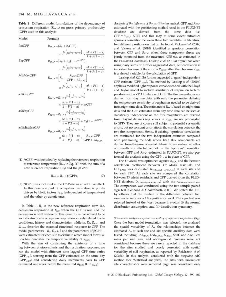
(1) f (GPP) was included by replacing the reference respiration

at reference temperature [Rref in Eq. (1)] with the sum of a

new reference respiration (R0) and the f(GPP):

Rref ¼ R0 þ f GPPð Þ: ð7Þ

(2) f (GPP) was included in the TP Model as an additive effect.

In this case one part of ecosystem respiration is purely

driven by biotic factors (e.g. independent of temperature)

and the other by abiotic ones.

In Table 1, R0 is the new reference respiration term (i.e.

ecosystem respiration at Tref, when the GPP is null and the

ecosystem is well watered). This quantity is considered to be

an indicator of site ecosystem respiration, closely related to site

conditions, history and characteristics, while k2, R2, Rmax and

hRmax describe the assumed functional response to GPP. The

model parameters – R0, E0, a, k and the parameters of f(GPP) –

were estimated for each site to evaluate which model formula-

tion best describes the temporal variability of RECO.

With the aim of confirming the existence of a time

lag between photosynthesis and the respiration response, we

ran the model with different time lagged GPP time series

(GPPlag,i), starting from the GPP estimated on the same day

(GPPlag,0) and considering daily increments back to GPP

estimated one week before the measured RECO (GPPlag,7).

Analysis of the influence of the partitioning method. GPP and RECO

estimated with the partitioning method used in the FLUXNET

database are derived from the same data (i.e.

GPP 5 RECO�NEE) and this may to some extent introduce

spurious correlation between these two variables. In literature,

two different positions on that can be found: Vickers et al. (2009)

and Vickers et al. (2010) identified a spurious correlation

between GPP and RECO when these component fluxes are

jointly estimated from the measured NEE (i.e. as estimated in

the FLUXNET database). Lasslop et al. (2010a) argue that when

using daily sums or further aggregated data, self-correlation is

important because of the error in RECO rather than because RECO

is a shared variable for the calculation of GPP.

Lasslop et al. (2010b) further suggested a ‘quasi’-independent

GPP estimate (GPPLASS). The method by Lasslop et al. (2010b)

applies a modified light response curve extended with the Lloyd

and Taylor model to include sensitivity of respiration to tem-

perature with a VPD limitation of GPP. The flux magnitudes are

derived from daytime data, with only the parameter defining

the temperature sensitivity of respiration needed to be derived

from night-time data. The estimates of RECO based on night-time

data and the GPP estimated from day-time data can be seen as

statistically independent as the flux magnitudes are derived

from disjoint datasets (e.g. errors in RECO are not propagated

to GPP). They are of course still subject to potential systematic

errors, but no constant error affects the correlation between the

two flux components. Hence, if existing, ‘spurious’ correlations

are minimized for the two independent estimates compared

with partitioning methods where both flux components are

derived from the same observed dataset. To understand whether

our results are affected or not by the ‘spurious’ correlation

between GPP and RECO estimated in FLUXNET, we also per-

formed the analysis using the GPPLASS in place of GPP.

The TP Model was optimized against RECO and the Pearson

correlation coefficient between TP Model residuals and

GPPLASS was calculated (rTPModel�GPPLASS) at each site and

for each PFT. At each site we compared the correlation

between TP Model residuals and GPP derived from the FLUX-

NET database (rTPModel�GPPFLUX) with the rTPModel�GPPLASS.

The comparison was conducted using the two sample paired

sign test (Gibbons & Chakraborti, 2003). We tested the null

hypothesis that the median of the difference between two

samples is zero, for a 1% significance level. The sign test was

selected instead of the t-test because it avoids: (i) the normal

distribution assumption; and (ii) distribution symmetry.

Site-by-site analysis – spatial variability of reference respiration (R0).Once the best model formulation was selected, we analyzed

the spatial variability of R0: the relationships between the

estimated R0 at each site and site-specific ancillary data were

tested, including LAIMAX, LAIMAX,o, Ndepo, SoilC and Age. Leaf

mass per unit area and aboveground biomass were not

considered because these are rarely reported in the database

for the sites studied and poorly correlated with spatial

variability of soil respiration, as reported by Reichstein et al.

(2003a). In this analysis, conducted with the stepwise AIC

method (see ‘Statistical analysis’), the sites with incomplete

site characteristics were removed (Age was considered only

Table 1 Different model formulations of the dependency of

ecosystem respiration (RECO) on gross primary productivity

(GPP) used in this analysis

Model Formula

LinGPP RECO ¼ R0 þ k2GPPð Þ

� eE0

1Tref�T0

� 1TA�T0

� �� akþ P 1� að Þ

kþ P 1� að ÞExpGPP RECO ¼ R0 þ R2 1� ek2GPP

� �� �

� eE0

1Tref�T0

� 1TA�T0

� �� akþ P 1� að Þ

kþ P 1� að ÞMicMenGPP

RECO ¼ R0 þRMAXGPP

GPPþ hRMAX

�

� eE0

1Tref�T0

� 1TA�T0

� �� akþ P 1� að Þ

kþ P 1� að ÞaddLinGPP

RECO ¼R0 � eE0

1Tref�T0

� 1TA�T0

� �

� akþ P 1� að Þkþ P 1� að Þ þ k2GPP

addExpGPPRECO ¼R0 � e

E01

Tref�T0� 1

TA�T0

� �

� akþ P 1� að Þkþ P 1� að Þ þ R2 1� ek2GPP

� �addMicMenGPP

RECO ¼R0 � eE0

1Tref�T0

� 1TA�T0

� �

� akþ P 1� að Þkþ P 1� að Þ þ

RMAXGPP

GPPþ hRMAX

394 M . M I G L I AVA C C A et al.

r 2010 Blackwell Publishing Ltd, Global Change Biology, 17, 390–409

for the analysis of forest ecosystems). On the basis of this

analysis the model was reformulated by adding the explicit

dependency of R0 on the site characteristics that best explained

its variability.

PFT-analysis. In this phase we tried to generalize the model

parameters to obtain a parameterization useful for diagnostic

PFT-based up-scaling. For this reason model parameters were

estimated including all the sites for each PFT at the same time.

The dependency of R0 was prescribed as a function of site

characteristics that best explain the spatial R0 variability

within each PFT class.

The model was corroborated with two different cross-

validation methods:

(1) Training/evaluation splitting cross-validation: one site at a

time was excluded using the remaining subset as the

training set and the excluded one as the validation set.

The model was fitted against each training set and the

resulting parameterization was used to predict the RECO of

the excluded site.

(2) k-fold cross-validation: the whole dataset for each PFT was

divided into k randomly selected subsets (k 5 15) called a

fold. The model was fitted against k�1 remaining folds

(training set) while the excluded fold (validation set) was

used for model evaluation. The cross-validation process

was then repeated k times, with each of the k-folds used

exactly once as the validation set.

For each validation set of the cross-validated model, statistics

were calculated (see ‘Statistical analysis’). Finally, for each PFT

we averaged the cross-validated statistics to produce a single

estimation of model accuracy in prediction.

Statistical analysis

Model parameter estimates. Model parameters were estimated

using the Levenberg–Marquardt method, implemented in the

data analysis package ‘PV-WAVE 8.5 ADVANTAGE’ (Visual Numerics,

2005), a nonlinear regression analysis that optimizes model

parameters finding the minimum of a defined cost function.

The cost function used here is the sum of squared residuals

weighted for the uncertainty of the observation (e.g. Richardson

& Hollinger, 2005). The uncertainty used here is an estimate of

the random error associated with the night-time fluxes (from

which RECO is derived).

Model parameter standard errors were estimated using a

bootstrapping algorithm with N 5 500 random resampling with

replacement of the dataset. As described by Efron & Tibshirani

(1993), the distribution of parameter estimates obtained provided

an estimate of the distribution of the true model parameters.

Best model formulation selection. For the selection of the ‘best’

model from among the six different formulations listed in Table 1

and the TP Model, we used the approach of the information

criterion developed by Akaike (1973) which is considered a useful

metric for model selection (Anderson et al., 2000; Richardson et al.,

2006). In this study the cAIC [Eqn (8)] was preferred to the AIC

because the latter is biased with large datasets (Shono, 2005),

tending to select more complicated models (e.g. many

explanatory variables exist in regression analysis):

cAIC ¼ �2 log L Yð Þ þ p log nð Þ þ 1� �

; ð8Þ

where L(Y) is the within-samples residual sum of squares, p is the

number of unknown parameters and n is the number of data (i.e.

sample size). Essentially, when the dimension of the dataset is

fixed, cAIC is a measure of the trade-off between the goodness of

fit (model explanatory power) and model complexity (number of

parameters), thus cAIC selects against models with an exces-

sive number of parameters. Given a dataset, several competing

models (e.g. different model formulations proposed in Table 1)

can be ranked according to their cAIC, with the formulation

having the lowest cAIC being considered the best according to

this approach.

For the selection of the best set of predictive variables for R0

we used the stepwise AIC, a multiple regression method for

variable selection based on the AIC criterion (Venables & Ripley,

2002; Yamashita et al., 2007). The stepwise AIC was preferred to

other stepwise methods for variable selection since it can be

applied to nonnormally distributed data (Yamashita et al., 2007).

Evaluation of model accuracy. Model accuracy was evaluated by

means of different statistics according to Janssen & Heuberger

(1995): root mean square error (RMSE), EF (modeling efficiency),

determination coefficient (r2) and mean absolute error (MAE). In

particular, EF is a measure of the coincidence between observed

and modeled data and it is sensitive to systematic deviation

between model and observations. EF can range from �1 to 1.

An EF of 1 corresponds to a perfect agreement between model

and observation. An EF of 0 indicates that the model is as

accurate as the mean of the observed data, whereas a negative

EF means that the observed mean is a better predictor than the

model. In the PFT analysis for each validation set the cross-

validated statistics were calculated. The averages of cross-

validated statistics were calculated for each PFT both for

training/evaluation splitting (EFcv, RMSEcv, r2cv) and for k-fold

cross-validation (EFkfold-cv, RMSEkfold-cv, r2kfold�cv).

Results

Site-by-site analysis

TP model results. The RMSE and EF obtained with TP

Model fitting (Table 2) showed a within-PFT-average EF

ranging from 0.38 for SAV to 0.71 for ENF and an RMSE

ranging from 0.67 for SHB to 1.55 g C m�2 day�1 for CRO.

The importance of productivity is highlighted by the

analysis of the residuals. A significant positive correlation

between the TP Model residuals (z) and the GPP was

observed with a systematic underestimation of respira-

tion when GPP was large.

In Fig. 2a, the mean rTPModel�GPPFLUX for each PFT as

a function of the time lag is summarized.

The lowest correlation was observed for wetlands

(r 5 0.29 � 0.14). The mean rTPModel�GPPFLUX is higher

for herbaceous ecosystems such as grasslands and

S E M I E M P I R I C A L M O D E L I N G O F E C O S Y S T E M R E S P I R A T I O N 395

r 2010 Blackwell Publishing Ltd, Global Change Biology, 17, 390–409

croplands (0.55 � 0.11 and 0.63 � 0.18, respectively)

than for forest ecosystems (ENF, DBF, MF, EBF), which

behaved in the same way (Fig. 2a), with values ranging

from 0.35 � 0.13 for ENF to 0.45 � 0.13 for EBF. No time

lag was observed with the analysis of residuals.

GPP as a driver of RECO. The effect of GPP as an

additional driver of RECO was analyzed at each site by

testing six different models (Table 1). The model

ranking based on the cAIC calculated for each

different model formulation at each site showed

agreement in considering the models using the linear

dependency of RECO on GPP (LinGPP) as the best model

formulation (Table 2), since the cAICs obtained with

LinGPP were lower than those obtained with all the

other formulations. This model ranking was also

maintained when analyzing each PFT separately,

except for croplands where the addLinGPP formulation

provided the minimum cAIC. It is notable that the

difference between the average cAIC estimated for the

two model formulations was almost negligible (cAIC was

38.22 � 2.52 and 38.26 � 2.45 for addLinGPP and LinGPP,

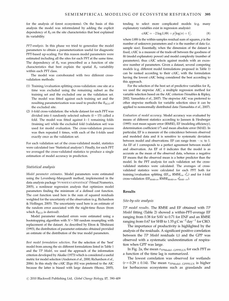
Table 2 Statistics of fit for the climate-driven model (TP Model) and the best model selected among the models listed in Table 1

according to the consistent Akaike Information Criterion (cAIC)

PFT

TP Model LinGPP Model

Best model selectedEF RMSE EF RMSE

ENF 0.71 (0.14) 1.02 (0.35) 0.78 (0.14) 0.83 (0.21) LinGPP

DBF 0.63 (0.17) 1.15 (0.51) 0.72 (0.13) 0.98 (0.41) LinGPP

GRA 0.62 (0.18) 1.35 (0.43) 0.83 (0.07) 0.91 (0.33) LinGPP

CRO 0.55 (0.18) 1.55 (0.53) 0.82 (0.08) 1.01 (0.33) addLinGPP

SAV 0.38 (0.16) 0.78 (0.24) 0.72 (0.06) 0.53 (0.15) LinGPP

SHB 0.59 (0.29) 0.67 (0.50) 0.66 (0.29) 0.58 (0.51) LinGPP

EBF 0.42 (0.27) 1.11 (0.55) 0.58 (0.23) 0.91 (0.49) LinGPP

MF 0.67 (0.18) 0.96 (0.72) 0.82 (0.13) 0.78 (0.50) LinGPP

WET 0.67 (0.18) 0.96 (0.51) 0.85 (0.48) 0.79 (0.07) LinGPP

Statistics are averaged per plant functional type (PFT). Except for croplands (CRO), LinGPP is selected as the best model formulation. EF

is the modeling efficiency while RMSE is the root mean square error (Jannsen and Heuberger, 1995). Values in brackets are the standard

deviations. The list of acronyms is also provided in Appendix S2.

The definitions of different PFTs are: evergreen needleleaf forest (ENF), deciduous broadleaf forest (DBF), grassland (GRA),

cropland (CRO), savanna (SAV), shrubland (SHB), evergreen broadleaf forest (EBF), mixed forest (MF) and wetland (WET).

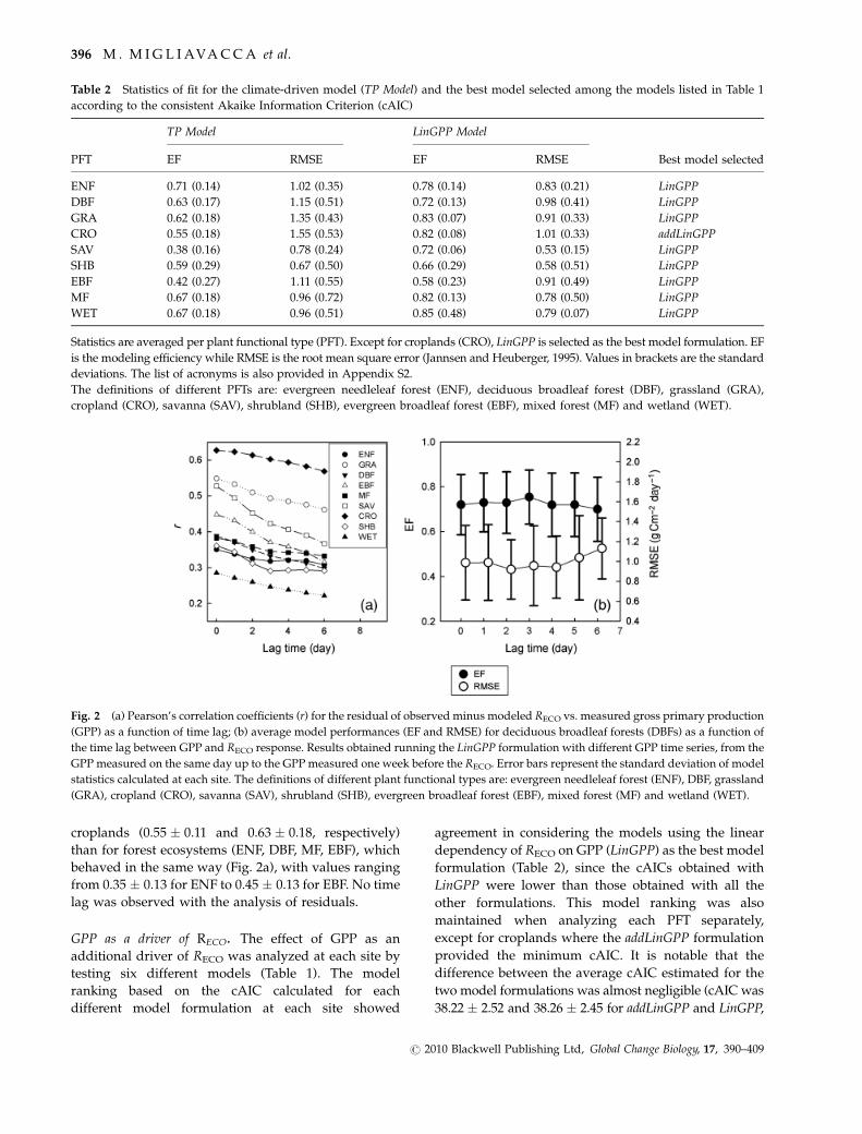
Fig. 2 (a) Pearson’s correlation coefficients (r) for the residual of observed minus modeled RECO vs. measured gross primary production

(GPP) as a function of time lag; (b) average model performances (EF and RMSE) for deciduous broadleaf forests (DBFs) as a function of

the time lag between GPP and RECO response. Results obtained running the LinGPP formulation with different GPP time series, from the

GPP measured on the same day up to the GPP measured one week before the RECO. Error bars represent the standard deviation of model

statistics calculated at each site. The definitions of different plant functional types are: evergreen needleleaf forest (ENF), DBF, grassland

(GRA), cropland (CRO), savanna (SAV), shrubland (SHB), evergreen broadleaf forest (EBF), mixed forest (MF) and wetland (WET).

396 M . M I G L I AVA C C A et al.

r 2010 Blackwell Publishing Ltd, Global Change Biology, 17, 390–409

respectively) and the standard errors of parameter

estimates were lower for the LinGPP formulation. In

general, the cAIC values obtained at all sites with the

LinGPP model formulation [39.50 (37.50–42.22), in

parenthesis the first and third quartile are reported]

were lower than the ones obtained with the TP Model

[41.08 (39.02–44.40)], although the complexity of the

latter was lower (one parameter less). On this basis

we considered the LinGPP as the best model

formulation.

The statistics of model fitting obtained with the

LinGPP model formulation are reported in Table 2.

The model optimized site by site showed a within-

PFT-average of EF between 0.58 for EBF and 0.85 for

WET with an RMSE ranging from 0.53 for SAV to

1.01 g C m�2 day�1 for CRO. On average, EF was

40.65 for all the PFTs except for EBF. In terms of

improvement of statistics, the use of LinGPP in the TP

Model led to a reduction of the RMSE from 13.4% for

shrublands to almost one-third for croplands (34.8%),

grasslands (32.5%) and savannas (32.0%) with respect to

the statistics corresponding to the purely climate-driven

TP Model.

No time lag between photosynthesis and respiration

response was detected. In fact, using GPPlag,�i as a

model driver we observed a general decrease in mean

model performances for each PFT (i.e. decrease in EF

and increase in RMSE) for increasing i values (i.e.

number of days in which the GPP was observed before

the observed RECO). The only exception was DBF in

which we found a time lag between the GPP and RECO

response of 3 days as shown by the peak in average EF

and by the minimum in RMSE in Fig. 2b, although these

differences were not statistically significant.

Analysis of the importance of ‘spurious’ correlation between

RECO and GPP. At each site we compared the correlation

between TP Model residuals and GPP included in

FLUXNET and the one computed by Lasslop et al.

(2010b). The paired sign test between rTPModel�GPPFLUX

and rTPModel�GPPLASS performed for each PFT indicates

that the median of the differences of the populations are

negligible for almost all the PFTs (Fig. 3 and Table 3).

The only exception was observed in tall canopies such

as ENF, MF and EBF, for which the differences were

statistically significant (Po0.01 for ENF and MF; Po0.05

for EBF). However, the rTPModel�GPPLASS is only slightly

lower than rTPModel�GPPFLUX: �0.035 for MF and �0.050

for ENF.

In conclusion, these results confirm that in this case

the bias observed in the purely climate driven model it

is not imputable to a ‘spurious’ correlation between

RECO and GPP introduced by the partitioning method

used in the FLUXNET database and that when using a

CRO DBF EBF ENF GRA MF SAV SHB WET

−1.0

−0.5

0.0

0.5

1.0

PFT

r TP

Mod

el–G

PP

LAS

S−r

TP

Mod

el−G

PP

FLU

X

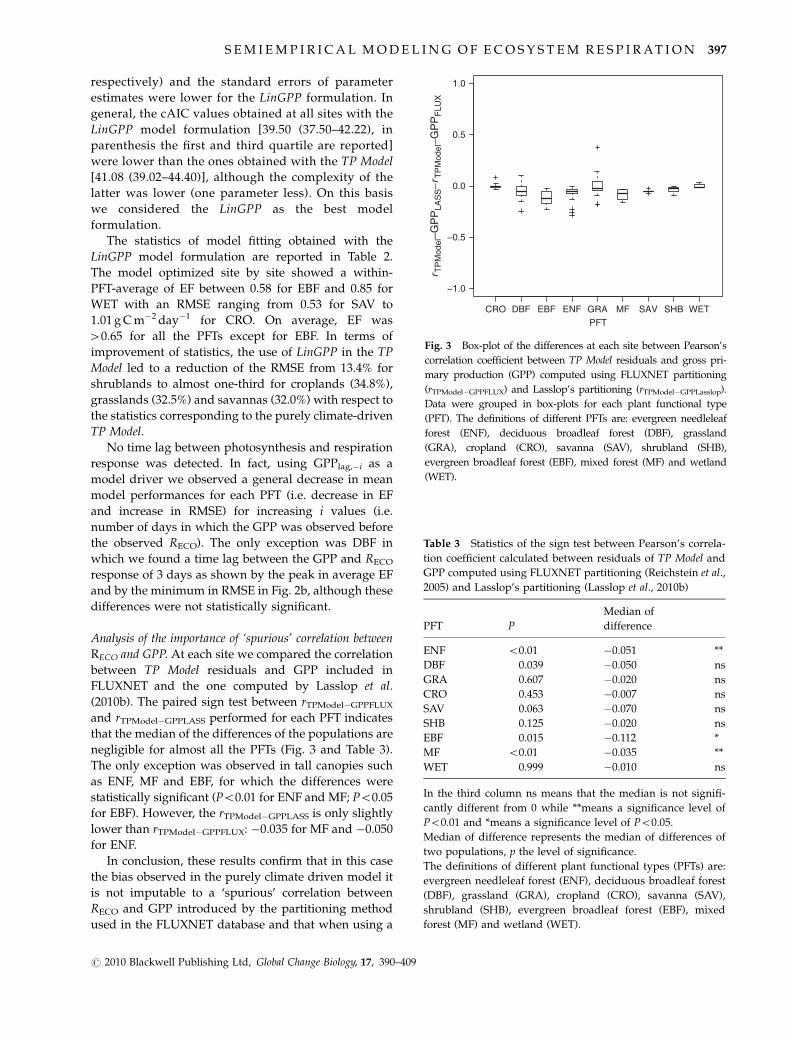
Fig. 3 Box-plot of the differences at each site between Pearson’s

correlation coefficient between TP Model residuals and gross pri-

mary production (GPP) computed using FLUXNET partitioning

(rTPModel�GPPFLUX) and Lasslop’s partitioning (rTPModel�GPPLasslop).

Data were grouped in box-plots for each plant functional type

(PFT). The definitions of different PFTs are: evergreen needleleaf

forest (ENF), deciduous broadleaf forest (DBF), grassland

(GRA), cropland (CRO), savanna (SAV), shrubland (SHB),

evergreen broadleaf forest (EBF), mixed forest (MF) and wetland

(WET).

Table 3 Statistics of the sign test between Pearson’s correla-

tion coefficient calculated between residuals of TP Model and

GPP computed using FLUXNET partitioning (Reichstein et al.,

2005) and Lasslop’s partitioning (Lasslop et al., 2010b)

PFT P

Median of

difference

ENF o0.01 �0.051 **

DBF 0.039 �0.050 ns

GRA 0.607 �0.020 ns

CRO 0.453 �0.007 ns

SAV 0.063 �0.070 ns

SHB 0.125 �0.020 ns

EBF 0.015 �0.112 *

MF o0.01 �0.035 **

WET 0.999 �0.010 ns

In the third column ns means that the median is not signifi-

cantly different from 0 while **means a significance level of

Po0.01 and *means a significance level of Po0.05.

Median of difference represents the median of differences of

two populations, p the level of significance.

The definitions of different plant functional types (PFTs) are:

evergreen needleleaf forest (ENF), deciduous broadleaf forest

(DBF), grassland (GRA), cropland (CRO), savanna (SAV),

shrubland (SHB), evergreen broadleaf forest (EBF), mixed

forest (MF) and wetland (WET).

S E M I E M P I R I C A L M O D E L I N G O F E C O S Y S T E M R E S P I R A T I O N 397

r 2010 Blackwell Publishing Ltd, Global Change Biology, 17, 390–409

quasi-independent estimate of GPP the overall meaning

of the results is the same.

Spatial variability of reference respiration rates. The

reference respiration rates (R0) estimated site by site

with the LinGPP model formulation represent daily

ecosystem respiration at each site at a reference

temperature (i.e. 15 1C), without water limitation

and carbon assimilation. Hence, R0 can be

considered the respiratory potential of a particular site.

R0 assumed the highest values for the ENF

(3.01 � 1.35 g C m�2 day�1) while the lowest values

were found for SHB (1.49 � 0.82 g C m�2 day�1) and

WET (1.11 � 0.17 g C m�2 day�1), possibly reflecting

lower carbon pools for shrublands or lower

decomposition rates due to anoxic conditions or

carbon stabilization for wetlands.

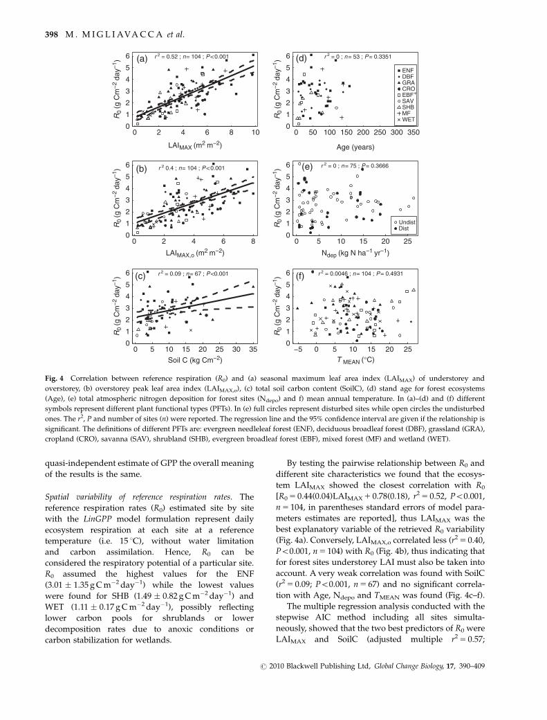
By testing the pairwise relationship between R0 and

different site characteristics we found that the ecosys-

tem LAIMAX showed the closest correlation with R0

[R0 5 0.44(0.04)LAIMAX 1 0.78(0.18), r2 5 0.52, Po0.001,

n 5 104, in parentheses standard errors of model para-

meters estimates are reported], thus LAIMAX was the

best explanatory variable of the retrieved R0 variability

(Fig. 4a). Conversely, LAIMAX,o correlated less (r2 5 0.40,

Po0.001, n 5 104) with R0 (Fig. 4b), thus indicating that

for forest sites understorey LAI must also be taken into

account. A very weak correlation was found with SoilC

(r2 5 0.09; Po0.001, n 5 67) and no significant correla-

tion with Age, Ndepo and TMEAN was found (Fig. 4c–f).

The multiple regression analysis conducted with the

stepwise AIC method including all sites simulta-

neously, showed that the two best predictors of R0 were

LAIMAX and SoilC (adjusted multiple r2 5 0.57;

0 2 4 6 8 100

1

2

3

4

5

6

LAIMAX (m2 m−2)

R0

(g C

m−

2 da

y–1)

0 2 4 6 80

1

2

3

4

5

6

LAIMAX,o (m2 m−2)

R0

(g C

m−

2 da

y–1)

0 5 10 15 20 25 30 350

1

2

3

4

5

6

Soil C (kg Cm−2)

R0

(g C

m−

2 da

y–1)

0 50 100 150 200 250 300 3500

1

2

3

4

5

6

Age (years)

R0

(g C

m−

2 da

y–1)

ENFDBFGRACROEBFSAVSHBMFWET

0 5 10 15 20 250

1

2

3

4

5

6

Ndep (kg N ha−1 yr−1)

R0

(g C

m−

2 da

y–1)

UndistDist

−5 0 5 10 15 20 250

1

2

3

4

5

6

T MEAN (°C)

R0

(g C

m−

2 da

y–1)

r = 0.52 ; n= 104 ; P <0.001

r 0.4 ; n= 104 ; P <0.001

r = 0.09 ; n= 67 ; P <0.001

r = 0 ; n= 53 ; P= 0.3351

r = 0 ; n= 75 ; P= 0.3666

r = 0.0046 ; n= 104 ; P= 0.4931

(a) (d)

(e)(b)

(c) (f)

Fig. 4 Correlation between reference respiration (R0) and (a) seasonal maximum leaf area index (LAIMAX) of understorey and

overstorey, (b) overstorey peak leaf area index (LAIMAX,o), (c) total soil carbon content (SoilC), (d) stand age for forest ecosystems

(Age), (e) total atmospheric nitrogen deposition for forest sites (Ndepo) and f) mean annual temperature. In (a)–(d) and (f) different

symbols represent different plant functional types (PFTs). In (e) full circles represent disturbed sites while open circles the undisturbed

ones. The r2, P and number of sites (n) were reported. The regression line and the 95% confidence interval are given if the relationship is

significant. The definitions of different PFTs are: evergreen needleleaf forest (ENF), deciduous broadleaf forest (DBF), grassland (GRA),

cropland (CRO), savanna (SAV), shrubland (SHB), evergreen broadleaf forest (EBF), mixed forest (MF) and wetland (WET).

398 M . M I G L I AVA C C A et al.

r 2010 Blackwell Publishing Ltd, Global Change Biology, 17, 390–409

Tab

le4

Res

ult

so

fm

od

else

lect

ion

con

du

cted

wit

hth

est

epw

ise

AIC

met

ho

dfo

rth

esi

tes

bel

on

gin

gto

all

the

pla

nt

fun

ctio

nal

typ

e(P

FT

)(A

llP

FT

s)an

dfo

ru

nd

istu

rbed

tem

per

ate

and

bo

real

fore

sts

iden

tifi

edin

Ap

pen

dix

S2

(Un

dis

turb

edF

ore

sts)

Mo

del

Bes

tm

od

else

lect

eda 1

a 2C

on

str2

r2 adju

sted

Pn

All

PF

Ts

R0

5a 1

LA

I MA

X1

a 2S

oil

C1

con

st0.

412

(0.0

48)*

**0.

045

(0.0

15)*

*0.

582

(0.2

51)*

0.58

0.57

o0.

001

68

Un

dis

turb

edF

ore

st(M

F1

DB

F1

EN

F)

R0

5a 1

LA

I MA

X1

a 2N

dep

o1

con

st0.

469

(0.0

69)*

**�

0.02

5(0

.017

)�

0.94

8(0

.377

)*0.

700.

67o

0.00

123

Dis

turb

edF

ore

sts

R0

5a 1

So

ilC

1a 2

TM

EA

N1

con

st0.

211

(0.0

51)*

*�

0.18

8(0

.059

)**

3.48

7(0

.982

)*0.

850.

80o

0.00

110

Co

effi

cien

ts(a

1,

a 2an

dco

nst

ant)

,th

eir

sig

nifi

can

cean

dth

est

atis

tics

of

the

bes

tm

od

else

lect

edar

ere

po

rted

.In

par

enth

eses

the

stan

dar

der

ror

of

coef

fici

ents

isre

po

rted

.T

he

sig

nifi

can

ceo

fco

effi

cien

tsis

also

rep

ort

ed(

*** P

o0.

001,

**Po

0.01

,* P

o0.

05,�

Po

0.1)

.

AIC

,A

kai

ke

Info

rmat

ion

Cri

teri

on

.

Tab

le5

Par

amet

ers

of

the

rela

tio

nsh

ips

bet

wee

nre

fere

nce

resp

irat

ion

(R0)

defi

ned

at15

1C

and

seas

on

alm

axim

um

LA

Ifo

rea

chp

lan

tfu

nct

ion

alty

pe

(PF

T)

PF

T

Par

amet

ers

and

stat

isti

cs(R

0v

s.L

AI M

AX)

Fin

alm

od

elp

aram

eter

sF

itti

ng

stat

isti

cs

RL

AI5

0a L

AI

r2P

k 2E

0(K

)a

K(m

m)

r2E

F

RM

SE

(gC

m�

2d

ay�

1)

MA

E

(gC

m�

2d

ay�

1)

EN

F1.

02(0

.42)

0.42

(0.0

8)0.

50o

0.00

10.

478

(0.0

13)

124.

833

(4.6

56)

0.60

4(0

.065

)0.

222

(0.0

70)

0.79

0.70

1.07

20.

788

DB

F1.

27(0

.50)

0.34

(0.1

0)0.

46o

0.01

0.24

7(0

.009

)87

.655

(4.4

05)

0.79

6(0

.031

)0.

184

(0.0

64)

0.65

0.52

1.32

20.

899

GR

A0.

41(0

.71)

1.14

(0.3

3)0.

60o

0.00

10.

578

(0.0

62)

101.

181

(6.3

62)

0.67

0(0

.052

)0.

765

(1.5

89)

0.82

0.80

1.08

30.

838

CR

O0.

25(0

.66)

0.40

(0.1

1)0.

52o

0.00

10.

244

(0.0

16)

129.

498

(5.6

18)

0.93

4(0

.065

)0.

035

(3.0

18)

0.80

0.79

0.93

30.

659

SA

V0.

42(0

.39)

0.57

(0.1

7)0.

54o

0.00

50.

654

(0.0

24)

81.5

37(7

.030

)0.

474

(0.0

18)

0.56

7(0

.119

)0.

650.

600.

757

0.53

5

SH

B0.

42(0

.39)

0.57

(0.1

7)0.

54o

0.00

50.

354

(0.0

21)

156.

746

(8.2

22)

0.85

0(0

.070

)0.

097

(1.3

04)

0.73

0.60

0.61

80.

464

EB

F�

0.47

(0.5

0)0.

82(0

.13)

0.87

o0.

001

0.60

2(0

.044

)52

.753

(4.3

51)

0.59

3(0

.032

)2.

019

(1.0

52)

0.55

0.41

1.00

20.

792

MF

0.78

(0.1

8)0.

44(0

.04)

0.52

o0.

001

0.39

1(0

.068

)17

6.54

2(8

.222

)0.

703

(0.0

83)

2.83

1(4

.847

)0.

860.

790.

988

0.72

3

WE

T0.

78(0

.18)

0.44

(0.0

4)0.

52o

0.00

10.

398

(0.0

13)

144.

705

(8.7

62)

0.58

2(0

.163

)0.

054

(0.5

93)

0.87

0.86

0.40

30.

292

Th

est

and

ard

erro

rso

fm

od

elp

aram

eter

sar

ere

po

rted

inp

aren

thes

es.

Det

erm

inat

ion

coef

fici

ents

and

stat

isti

cal

sig

nifi

can

cear

eal

sosh

ow

n.

TP

GP

P-L

AI

Mod

elp

aram

eter

s

esti

mat

edfo

rea

chp

lan

tfu

nct

ion

alty

pe

(see

Ap

pen

dix

S2)

.S

tan

dar

der

rors

esti

mat

edw

ith

the

bo

ots

trap

alg

ori

thm

are

rep

ort

edin

par

enth

eses

.T

PG

PP

-LA

IM

odel

isd

efin

edin

Eq

n(9

).T

he

defi

nit

ion

so

fd

iffe

ren

tP

FT

sar

e:ev

erg

reen

nee

dle

leaf

fore

st(E

NF

),d

ecid

uo

us

bro

adle

affo

rest

(DB

F),

gra

ssla

nd

(GR

A),

cro

pla

nd

(CR

O),

sav

ann

a(S

AV

),sh

rub

lan

d

(SH

B),

ever

gre

enb

road

leaf

fore

st(E

BF

),m

ixed

fore

st(M

F)

and

wet

lan

d(W

ET

).

S E M I E M P I R I C A L M O D E L I N G O F E C O S Y S T E M R E S P I R A T I O N 399

r 2010 Blackwell Publishing Ltd, Global Change Biology, 17, 390–409

Po0.001; n 5 68) which were both positively correlated

with R0 (Table 4). LAIMAX was the best predictor of

spatial variability of R0 for all sites, thus confirming the

results of the aforementioned pairwise regression ana-

lysis, but the linear model that included SoilC as an

additional predictor led to a significant, though small,

reduction in the AIC during the stepwise procedure.

Considering only the undisturbed temperate and

boreal forest sites (ENF, DBF, MF), the predictive vari-

ables of R0 selected were LAIMAX and Ndepo (adjusted

multiple r2 5 0.67; Po0.001; n 5 23). For these sites both

LAIMAX, which was still the main predictor of spatial

variability of R0, and Ndepo controlled the spatial varia-

bility of R0, with Ndepo negatively correlated to R0

(Table 4). This means that for these sites, once having

removed the effect of LAIMAX, Ndepo showed a negative

control on R0 with a reduction of 0.025 g C m�2 day�1 in

reference respiration for an increase of 1 kg N ha�1 yr�1

in total nitrogen depositions. Considering only the

disturbed forest sites, we found that SoilC and TMEAN

were the best predictors of the spatial variability of R0

(adjusted multiple r2 5 0.80, Po0.001, n 5 10).

In Table 5 the statistics of the pairwise regression

analysis between R0 and LAIMAX for each PFT are

reported. The best fitting was obtained with the linear

relationship for all PFTs except for deciduous forests for

which the best fitting was obtained with the exponential

relationship R0 5 RLAI 5 0(1�e�aLAI).

PFT-analysis

Final formulation of the model. On the basis of the afore-

mentioned results, GPP as well as the linear dependency

between R0 and LAIMAX were included in the TP Model,

thus leading to a new model formulation [Eqn (9)]. The

final formulation is basically the TP Model with the

addition of biotic drivers (daily GPP and LAIMAX) and

hereafter referred to as TPGPP-LAI Model, where GPP

and LAIMAX reflect the inclusion of the biotic drivers in

the climate-driven model:

RECO ¼ RLAI¼0 þ aLAI � LAIMAX|fflfflfflfflfflfflfflfflfflfflfflfflfflfflfflfflfflfflfflfflffl{zfflfflfflfflfflfflfflfflfflfflfflfflfflfflfflfflfflfflfflfflffl}R0

þk2GPP

0@

1A

� eE0

1Tref�T0

� 1TA�T0

� �� akþ P 1� að Þ

kþ P 1� að Þ

; ð9Þ

where the term, RLAI 5 0 1 aLAI LAIMAX, describes the

dependency of the basal rate of respiration (R0 in Table

1) on site maximum seasonal ecosystem LAI. Although

we found that SoilC and Ndepo may help to explain the

spatial variability of R0, in the final model formulation

we included only the LAIMAX. The model is primarily

oriented to the up-scaling and spatial distribution

information of SoilC, Ndepo and disturbance may be

difficult to gather and is usually affected by high

uncertainty.

The parameters RLAI 5 0 and aLAI listed in Table 5

were introduced as fixed parameters in the TPGPP-LAI

Model. For wetlands and mixed forests the overall

relationship between LAIMAX and R0 was used. For

wetlands, available sites were insufficient to construct

a statistically significant relationship, while for mixed

forests the relationship was not significant (P 5 0.146).

PFT specific model parameters (k2, E0, k, a) of the

TPGPP-LAI Model were then derived using all data

from each PFT at the same time and listed with their

relative standard errors in Table 5. No significant differ-

ences in parameter values were found when estimating

all the parameters simultaneously (aLAI, RLAI 5 0,

k2, E0, k, a).

The scatterplots of the observed vs. modeled annual

sums of RECO are shown in Fig. 5, while results and

statistics are summarized in Table 6. The model was

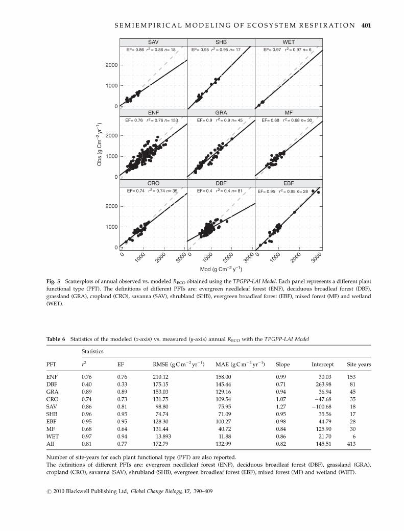
able to describe the interannual and intersite vari-

ability of the annual sums over different PFTs, with

the explained variance varying between 40% for DBF

and 97% for SHB and EBF. Considering all sites,

the explained variance is 81%, with a mean error of

about 17% (132.99 g C m�2 yr�1) of the annual observed

RECO.

Evaluation of model prediction accuracy and weak points.

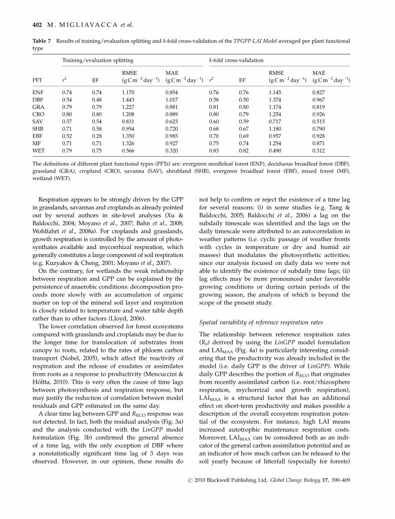
The results obtained with the k-fold and training/

evaluation split cross-validation are listed in Table 7.

The r2cv ranges from 0.52 (for EBF) to 0.80 (for CRO)

while the rcv,kfold2 ranges from 0.58 (for DBF) to 0.83 (for

WET). The cross-validated statistics averaged for each

PFT are in all cases higher for the k-fold than for the

training/evaluation splitting cross-validation.

The analysis of model residual time series of the DBF

(Fig. 6) showed a systematic underestimation during

the springtime development phase and, although less

clear, on the days immediately after leaf-fall. A similar

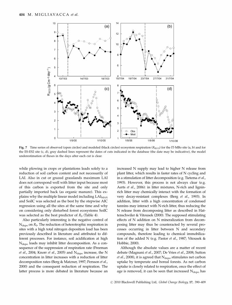
behavior was also found for croplands and grasslands

during the days after harvesting or cuts (Fig. 7).

Discussion

GPP as a driver of ecosystem respiration

The results obtained with the purely climate-driven

model (TP Model) and the best model formulation

selected in the site-by-site analysis (i.e. LinGPP,

Table 1) confirm the strong relationship between carbon

assimilation and RECO, thus highlighting that this rela-

tionship must be included in models aimed at simulat-

ing the temporal variability of RECO.

400 M . M I G L I AVA C C A et al.

r 2010 Blackwell Publishing Ltd, Global Change Biology, 17, 390–409

Mod (g Cm–2 y–1)

Obs

(g

Cm

–2 y

r–1)

0

1000

2000

010

0020

0030

00

CRO

010

0020

0030

00

DBF

010

0020

0030

00

EBF0

1000

2000

ENF GRA MF0

1000

2000

SAV SHB WET

EF= 0.76 = 0.76 n= 153 EF= 0.9 = 0.9 n= 45 EF= 0.68 = 0.68 n= 30

EF= 0.86 = 0.86 n= 18 EF= 0.95 = 0.95 n= 17 EF= 0.97 = 0.97 n= 6

EF= 0.74 = 0.74 n= 35 EF= 0.4 = 0.4 n= 81 EF= 0.95 = 0.95 n= 28

Fig. 5 Scatterplots of annual observed vs. modeled RECO obtained using the TPGPP-LAI Model. Each panel represents a different plant

functional type (PFT). The definitions of different PFTs are: evergreen needleleaf forest (ENF), deciduous broadleaf forest (DBF),

grassland (GRA), cropland (CRO), savanna (SAV), shrubland (SHB), evergreen broadleaf forest (EBF), mixed forest (MF) and wetland

(WET).

Table 6 Statistics of the modeled (x-axis) vs. measured (y-axis) annual RECO with the TPGPP-LAI Model

PFT

Statistics

r2 EF RMSE (g C m�2 yr�1) MAE (g C m�2 yr�1) Slope Intercept Site years

ENF 0.76 0.76 210.12 158.00 0.99 30.03 153

DBF 0.40 0.33 175.15 145.44 0.71 263.98 81

GRA 0.89 0.89 153.03 129.16 0.94 36.94 45

CRO 0.74 0.73 131.75 109.54 1.07 �47.68 35

SAV 0.86 0.81 98.80 75.95 1.27 �100.68 18

SHB 0.96 0.95 74.74 71.09 0.95 35.56 17

EBF 0.95 0.95 128.30 100.27 0.98 44.79 28

MF 0.68 0.64 131.44 40.72 0.84 125.90 30

WET 0.97 0.94 13.893 11.88 0.86 21.70 6

All 0.81 0.77 172.79 132.99 0.82 145.51 413

Number of site-years for each plant functional type (PFT) are also reported.

The definitions of different PFTs are: evergreen needleleaf forest (ENF), deciduous broadleaf forest (DBF), grassland (GRA),

cropland (CRO), savanna (SAV), shrubland (SHB), evergreen broadleaf forest (EBF), mixed forest (MF) and wetland (WET).

S E M I E M P I R I C A L M O D E L I N G O F E C O S Y S T E M R E S P I R A T I O N 401

r 2010 Blackwell Publishing Ltd, Global Change Biology, 17, 390–409

Respiration appears to be strongly driven by the GPP

in grasslands, savannas and croplands as already pointed

out by several authors in site-level analyses (Xu &

Baldocchi, 2004; Moyano et al., 2007; Bahn et al., 2008;

Wohlfahrt et al., 2008a). For croplands and grasslands,

growth respiration is controlled by the amount of photo-

synthates available and mycorrhizal respiration, which

generally constitutes a large component of soil respiration

(e.g. Kuzyakov & Cheng, 2001; Moyano et al., 2007).

On the contrary, for wetlands the weak relationship

between respiration and GPP can be explained by the

persistence of anaerobic conditions: decomposition pro-

ceeds more slowly with an accumulation of organic

matter on top of the mineral soil layer and respiration

is closely related to temperature and water table depth

rather than to other factors (Lloyd, 2006).

The lower correlation observed for forest ecosystems

compared with grasslands and croplands may be due to

the longer time for translocation of substrates from

canopy to roots, related to the rates of phloem carbon

transport (Nobel, 2005), which affect the reactivity of

respiration and the release of exudates or assimilates

from roots as a response to productivity (Mencuccini &

Holtta, 2010). This is very often the cause of time lags

between photosynthesis and respiration response, but

may justify the reduction of correlation between model

residuals and GPP estimated on the same day.

A clear time lag between GPP and RECO response was

not detected. In fact, both the residual analysis (Fig. 3a)

and the analysis conducted with the LinGPP model

formulation (Fig. 3b) confirmed the general absence

of a time lag, with the only exception of DBF where

a nonstatistically significant time lag of 3 days was

observed. However, in our opinion, these results do

not help to confirm or reject the existence of a time lag

for several reasons: (i) in some studies (e.g. Tang &

Baldocchi, 2005; Baldocchi et al., 2006) a lag on the

subdaily timescale was identified and the lags on the

daily timescale were attributed to an autocorrelation in

weather patterns (i.e. cyclic passage of weather fronts

with cycles in temperature or dry and humid air

masses) that modulates the photosynthetic activities;

since our analysis focused on daily data we were not

able to identify the existence of subdaily time lags; (ii)

lag effects may be more pronounced under favorable

growing conditions or during certain periods of the

growing season, the analysis of which is beyond the

scope of the present study.

Spatial variability of reference respiration rates

The relationship between reference respiration rates

(R0) derived by using the LinGPP model formulation

and LAIMAX (Fig. 4a) is particularly interesting consid-

ering that the productivity was already included in the

model (i.e. daily GPP is the driver of LinGPP). While

daily GPP describes the portion of RECO that originates

from recently assimilated carbon (i.e. root/rhizosphere

respiration, mychorrizal and growth respiration),

LAIMAX is a structural factor that has an additional

effect on short-term productivity and makes possible a

description of the overall ecosystem respiration poten-

tial of the ecosystem. For instance, high LAI means

increased autotrophic maintenance respiration costs.

Moreover, LAIMAX can be considered both as an indi-

cator of the general carbon assimilation potential and as

an indicator of how much carbon can be released to the

soil yearly because of litterfall (especially for forests)

Table 7 Results of training/evaluation splitting and k-fold cross-validation of the TPGPP-LAI Model averaged per plant functional

type

PFT

Training/evaluation splitting k-fold cross-validation

r2 EF

RMSE

(g C m�2 day�1)

MAE

(g C m�2 day�1) r2 EF

RMSE

(g C m�2 day�1)

MAE

(g C m�2 day�1)

ENF 0.74 0.74 1.170 0.854 0.76 0.76 1.145 0.827

DBF 0.54 0.48 1.443 1.017 0.58 0.50 1.374 0.967

GRA 0.79 0.79 1.227 0.881 0.81 0.80 1.174 0.819

CRO 0.80 0.80 1.208 0.889 0.80 0.79 1.254 0.926

SAV 0.57 0.54 0.831 0.623 0.60 0.59 0.717 0.515

SHB 0.71 0.58 0.954 0.720 0.68 0.67 1.180 0.790

EBF 0.52 0.28 1.350 0.985 0.70 0.69 0.957 0.928

MF 0.71 0.71 1.326 0.927 0.75 0.74 1.254 0.871

WET 0.79 0.75 0.566 0.320 0.83 0.82 0.490 0.312

The definitions of different plant functional types (PFTs) are: evergreen needleleaf forest (ENF), deciduous broadleaf forest (DBF),

grassland (GRA), cropland (CRO), savanna (SAV), shrubland (SHB), evergreen broadleaf forest (EBF), mixed forest (MF),

wetland (WET).

402 M . M I G L I AVA C C A et al.

r 2010 Blackwell Publishing Ltd, Global Change Biology, 17, 390–409

and leaf turnover, which are directly related to basal soil

respiration (Moyano et al., 2007). At recently disturbed

sites, this equilibrium between LAIMAX and soil carbon

(through litter inputs) may be broken, for example,

thinning might lead to a reduction of LAIMAX without

any short-term effect on the amount of soil carbon,

Fig. 6 Time series of average monthly model residuals for different deciduous broadleaf forest (DBF) sites. The vertical gray dashed

lines represent the phenological dates. Average phenological dates were derived for US-Ha1 from literature (Jolly et al., 2005) while for

other sites they were retrieved from the FLUXNET database. Average phenological dates, bud-burst and end-of-growing season are

respectively: US-Ha1 (115–296), DE-Hai (126–288), FR-Hes (120–290), FR-Fon (125–292), IT-Ro1 (104–298) and CA-Oas (146–258).

S E M I E M P I R I C A L M O D E L I N G O F E C O S Y S T E M R E S P I R A T I O N 403

r 2010 Blackwell Publishing Ltd, Global Change Biology, 17, 390–409

while plowing in crops or plantations leads solely to a

reduction of soil carbon content and not necessarily of

LAI. Also in cut or grazed grasslands maximum LAI

does not correspond well with litter input because most

of this carbon is exported from the site and only

partially imported back (as organic manure). This ex-

plains why the multiple linear model including LAIMAX

and SoilC was selected as the best by the stepwise AIC

regression using all the sites at the same time and why

on considering only disturbed forest ecosystems SoilC

was selected as the best predictor of R0 (Table 4).

Also particularly interesting is the negative control of

Ndepo on R0. The reduction of heterotrophic respiration in

sites with a high total nitrogen deposition load has been

previously described in literature and attributed to dif-

ferent processes. For instance, soil acidification at high

Ndepo loads may inhibit litter decomposition. As a con-

sequence of the suppression of respiration rate (Freeman

et al., 2004; Knorr et al., 2005) and Ndepo increase, the N

concentration in litter increases with a reduction of litter

decomposition rates (Berg & Matzner, 1997; Persson et al.,

2000) and the consequent reduction of respiration. The

latter process is more debated in literature because an

increased N supply may lead to higher N release from

plant litter, which results in faster rates of N cycling and

in a stimulation of litter decomposition (e.g. Tietema et al.,

1993). However, this process is not always clear (e.g.

Aerts et al., 2006): in litter mixtures, N-rich and lignin-

rich litter may chemically interact with the formation of

very decay-resistant complexes (Berg et al., 1993). In

addition, litter with a high concentration of condensed

tannins may interact with N-rich litter, thus reducing the

N release from decomposing litter as described in Hat-

tenschwiler & Vitousek (2000). The supposed stimulating

effects of N addition on N mineralization from decom-

posing litter may thus be counteracted by several pro-

cesses occurring in litter between N and secondary

compounds, therefore leading to chemical immobiliza-

tion of the added N (e.g. Pastor et al., 1987; Vitousek &

Hobbie, 2000).

Although the absolute values are a matter of recent

debate (Magnani et al., 2007; De Vries et al., 2008; Sutton

et al., 2008), it is agreed that Ndepo stimulates net carbon

uptake by temperate and boreal forests. As net carbon

uptake is closely related to respiration, once the effect of

age is removed, it can be seen that increased Ndepo has

Fig. 7 Time series of observed (open circles) and modeled (black circles) ecosystem respiration (RECO) for the IT-MBo site (a, b) and for

the ES-ES2 site (c, d), gray dashed lines represent the dates of cuts indicated in the database (the date may be indicative), the model

underestimation of fluxes in the days after each cut is clear.

404 M . M I G L I AVA C C A et al.

r 2010 Blackwell Publishing Ltd, Global Change Biology, 17, 390–409

the potential to drive RECO in either direction. The

stimulation of GPP as a consequence of increasing Ndepo

is already included in the model since GPP is a driver.

Additionally, our analysis suggests that on the whole an

increased total Ndepo in forests tends to reduce reference

respiration. Without considering the effects introduced

by Ndepo in our models we may overestimate RECO,

with a consequent underestimation of the carbon sink

strength of such terrestrial ecosystems. It is also clear

that in managed sites such interactions apply equally to

other anthropogenic nitrogen inputs (fertilizers, animal

excreta) (cf. Galloway et al., 2008; Janssens et al., 2010).

However, considering (i) that LAIMAX is the most

important predictor of R0, (ii) that the uncertainty in

soil carbon and total nitrogen deposition maps is usual-

ly high, (iii) that the spatial information on disturbance

is often lacking and finally (iv) that our model formula-

tion is oriented to up-scaling issues, we introduced

LAIMAX as the only robust predictor of the spatial

variability of R0 in the final model formulation. The

use of LAIMAX is useful from an up-scaling perspec-

tive (e.g. at regional or global scale) as it can be derived

by remotely sensed vegetation indices (e.g. normalized

vegetation index or enhanced vegetation index) thus

opening interesting perspectives for the assimilation of

remote sensing products in the TPGPP-LAI Model.

The intercepts of the PFT-based linear regression

between R0 and LAIMAX (Table 5) suggest that when

the LAIMAX is close to 0 (‘ideally’ bare soil) the lowest R0

takes place in arid (e.g. EBF) and agricultural ecosys-

tems. The frequent disturbances of agricultural soils (i.e.

plowing and tillage), as well as management, reduce

soil carbon content dramatically. In croplands, the esti-

mated R0 is very low in sites with low LAI. However,

with increasing LAIMAX, R0 shows a rapid increase, thus

resulting in high respiration rates for crop sites with

high LAI. For SHB and SAV the retrieved slopes are

typical of forest ecosystems, while the intercepts are

close to zero because of the lower soil carbon content

usually found in these PFTs (Raich & Schlesinger, 1992).

Because of the few available sites representing savannas

and shrublands, these were grouped on the basis of

climatic characteristics.

In grasslands, the steeper slope (aLAI) value found

(1.14 � 0.33) suggests that R0 increases rapidly with

increasing aboveground biomass as already pointed

out in literature (Wohlfahrt et al., 2005a, b, 2008a), i.e.

an increase in LAIMAX leads to a stronger increase in R0

than in other PFTs.

In forest ecosystems, and in particular in ENF and DBF,

the physical meaning of the higher intercept may reflect

the fact that transient soil carbon sources and sinks

dampen the interannual variability of RECO. For boreal

and high latitude forests another hypothesis is that these

ecosystems may be recovering from fire within the last

century or two, which means that variation in LAIMAX

across sites has more to do with how quickly carbon

stocks are reaccumulating than rates of RECO. In other

words, most boreal forests have some threshold main-

tenance respiration rate, and excess GPP beyond that

respiration rate goes toward biomass growth and reaccu-

mulation of surface layers of soil carbon. Thus, variations

in LAIMAX are less well correlated with RECO than they

are where recovery from previous stand-clearing fires or

other disturbances is less important (i.e. at lower lati-

tudes). This hypothesis is also supported by the lower r2

reported in Table 5 for DBF and ENF.

Final formulation of the model and weak points

The results obtained through cross-validation of the

TPGPP-LAI Model indicate that the developed model

describes RECO quite well. In particular, results indicate

a better description of the temporal variability of RECO

rather than the spatial variability (or across-site varia-

bility), in the light of the poorer results of the training/

evaluation splitting (in which one site at a time is

removed) compared with the k-fold cross-validation.

The derived parameterization of the TPGPP-LAI Model

reported in Table 5 may be considered as an optimized

parameterization for the application of the model at large

scale (e.g. continental or global). For this application it is

300 10 20 40

0.5

0.6

0.7

0.8

0.9

1.0

Daily precipitation (mm)

f (P

)

Fig. 8 Response function of ecosystem respiration to the 30-day

running average of daily precipitation [Eqn (2)] for each plant

functional type (PFT). The parameters in Table 4 were used to draw

the curves. The definitions of different PFTs are: evergreen needle-

leaf forest (ENF), deciduous broadleaf forest (DBF), grassland

(GRA), cropland (CRO), savanna (SAV), shrubland (SHB), ever-

green broadleaf forest (EBF), mixed forest (MF) and wetland (WET).

S E M I E M P I R I C A L M O D E L I N G O F E C O S Y S T E M R E S P I R A T I O N 405

r 2010 Blackwell Publishing Ltd, Global Change Biology, 17, 390–409

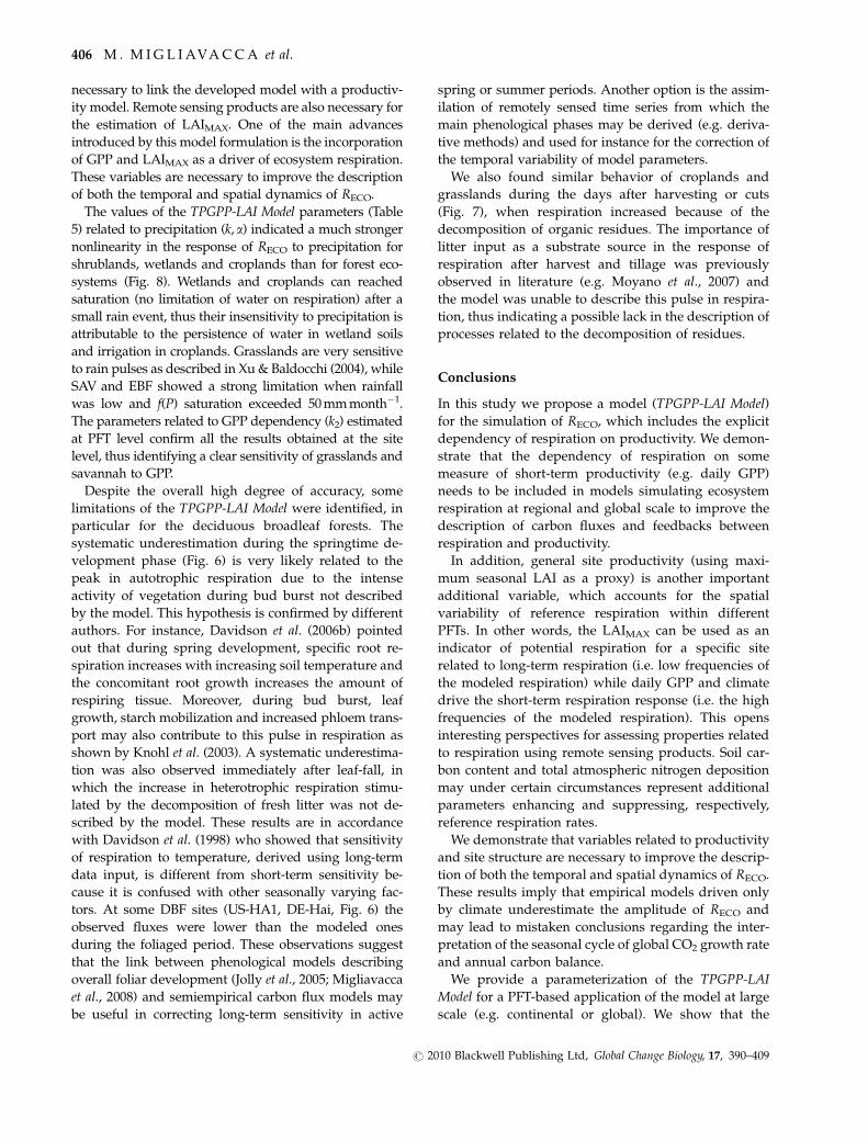
necessary to link the developed model with a productiv-

ity model. Remote sensing products are also necessary for

the estimation of LAIMAX. One of the main advances

introduced by this model formulation is the incorporation

of GPP and LAIMAX as a driver of ecosystem respiration.

These variables are necessary to improve the description

of both the temporal and spatial dynamics of RECO.

The values of the TPGPP-LAI Model parameters (Table

5) related to precipitation (k,a) indicated a much stronger

nonlinearity in the response of RECO to precipitation for

shrublands, wetlands and croplands than for forest eco-

systems (Fig. 8). Wetlands and croplands can reached

saturation (no limitation of water on respiration) after a

small rain event, thus their insensitivity to precipitation is

attributable to the persistence of water in wetland soils

and irrigation in croplands. Grasslands are very sensitive

to rain pulses as described in Xu & Baldocchi (2004), while

SAV and EBF showed a strong limitation when rainfall

was low and f(P) saturation exceeded 50 mm month�1.

The parameters related to GPP dependency (k2) estimated

at PFT level confirm all the results obtained at the site

level, thus identifying a clear sensitivity of grasslands and

savannah to GPP.

Despite the overall high degree of accuracy, some

limitations of the TPGPP-LAI Model were identified, in

particular for the deciduous broadleaf forests. The

systematic underestimation during the springtime de-

velopment phase (Fig. 6) is very likely related to the

peak in autotrophic respiration due to the intense

activity of vegetation during bud burst not described

by the model. This hypothesis is confirmed by different

authors. For instance, Davidson et al. (2006b) pointed

out that during spring development, specific root re-

spiration increases with increasing soil temperature and

the concomitant root growth increases the amount of

respiring tissue. Moreover, during bud burst, leaf

growth, starch mobilization and increased phloem trans-

port may also contribute to this pulse in respiration as

shown by Knohl et al. (2003). A systematic underestima-

tion was also observed immediately after leaf-fall, in

which the increase in heterotrophic respiration stimu-

lated by the decomposition of fresh litter was not de-

scribed by the model. These results are in accordance

with Davidson et al. (1998) who showed that sensitivity

of respiration to temperature, derived using long-term

data input, is different from short-term sensitivity be-

cause it is confused with other seasonally varying fac-

tors. At some DBF sites (US-HA1, DE-Hai, Fig. 6) the

observed fluxes were lower than the modeled ones

during the foliaged period. These observations suggest

that the link between phenological models describing

overall foliar development (Jolly et al., 2005; Migliavacca

et al., 2008) and semiempirical carbon flux models may

be useful in correcting long-term sensitivity in active

spring or summer periods. Another option is the assim-

ilation of remotely sensed time series from which the

main phenological phases may be derived (e.g. deriva-

tive methods) and used for instance for the correction of

the temporal variability of model parameters.

We also found similar behavior of croplands and

grasslands during the days after harvesting or cuts

(Fig. 7), when respiration increased because of the

decomposition of organic residues. The importance of

litter input as a substrate source in the response of

respiration after harvest and tillage was previously

observed in literature (e.g. Moyano et al., 2007) and

the model was unable to describe this pulse in respira-

tion, thus indicating a possible lack in the description of

processes related to the decomposition of residues.

Conclusions

In this study we propose a model (TPGPP-LAI Model)

for the simulation of RECO, which includes the explicit

dependency of respiration on productivity. We demon-

strate that the dependency of respiration on some

measure of short-term productivity (e.g. daily GPP)

needs to be included in models simulating ecosystem

respiration at regional and global scale to improve the

description of carbon fluxes and feedbacks between

respiration and productivity.

In addition, general site productivity (using maxi-

mum seasonal LAI as a proxy) is another important

additional variable, which accounts for the spatial

variability of reference respiration within different

PFTs. In other words, the LAIMAX can be used as an

indicator of potential respiration for a specific site

related to long-term respiration (i.e. low frequencies of

the modeled respiration) while daily GPP and climate

drive the short-term respiration response (i.e. the high

frequencies of the modeled respiration). This opens

interesting perspectives for assessing properties related

to respiration using remote sensing products. Soil car-

bon content and total atmospheric nitrogen deposition

may under certain circumstances represent additional

parameters enhancing and suppressing, respectively,

reference respiration rates.

We demonstrate that variables related to productivity

and site structure are necessary to improve the descrip-

tion of both the temporal and spatial dynamics of RECO.

These results imply that empirical models driven only

by climate underestimate the amplitude of RECO and

may lead to mistaken conclusions regarding the inter-

pretation of the seasonal cycle of global CO2 growth rate

and annual carbon balance.

We provide a parameterization of the TPGPP-LAI

Model for a PFT-based application of the model at large

scale (e.g. continental or global). We show that the

406 M . M I G L I AVA C C A et al.

r 2010 Blackwell Publishing Ltd, Global Change Biology, 17, 390–409

temporal, spatial and interannual variability of ecosys-

tem respiration can be captured well by the proposed

model. For this application a link of the developed

model with a productivity model is necessary (for

GPP estimation) as well as remote sensing products

(necessary for the estimation of LAI). One future per-

spective is the integration of the proposed model for-

mulation into the MODIS-GPP/NPP data stream (e.g.

MOD17 Light Use Efficiency model) for regional and

global estimates of RECO.

Finally, we observe that a part of ecosystem respira-

tion variance not explained by the model may be related

to phenology in deciduous forests and to management

in grasslands and croplands. For these reasons we

consider the link between phenological and respiration

models, as well as the inclusion of total nitrogen deposi-

tion and soil carbon stock, as additional drivers for

improving the description of ecosystem respiration in

both space and time.

Acknowledgements

The authors would like to thank all the PIs of eddy-covariancesites, technicians, postdoctoral fellows, research associates andsite collaborators involved in FLUXNET who are not included ascoauthors of this paper, without whose work this analysis wouldnot have been possible. This work is the outcome of the LaThuile FLUXNET Workshop 2007, which would not have beenpossible without the financial support provided by CarboEur-opeIP, FAO-GTOS-TCO, iLEAPS, Max Planck Institute for Bio-geochemistry, National Science Foundation, University of Tusciaand the US Department of Energy. Moreover, we acknowledgedatabasing and technical support from Berkeley Water Center,Lawrence Berkeley National Laboratory, Microsoft ResearcheScience, Oak Ridge National Laboratory, University of Califor-nia-Berkeley and University of Virginia. The following networksparticipated with flux data: AmeriFlux, AfriFlux, AsiaFlux,CarboAfrica, CarboEuropeIP, ChinaFlux, Fluxnet-Canada,KoFlux, LBA, NECC, OzFlux, TCOS-Siberia and USCCC. Amer-iFlux grant: US Department of Energy, Biological and Environ-mental Research and Terrestrial Carbon Program (DE-FG02-04ER63917). Data collection for the US-ARM sites was supportedby the Office of Biological and Environmental Research of the USDepartment of Energy under contract DE-AC02-05CH11231 aspart of the Atmospheric Radiation Measurement Program. M. A.S contribution was supported by the Nitro-Europe Project. M. M.was supported by the University of Milano-Bicocca and by theModel-Data Integration Group of the Max-Planck Institute forBiogeochemistry. M. M. acknowledges the Remote Sensing forEnvironmental Dynamics Laboratory, LTDA (in particular L.Busetto, M. Meroni and M. Rossini), C. Beer and M. Jung fromthe Max-Planck Institute for Biogeochemistry for the fruitfuldiscussions during the data analysis. M. R. acknowledges fund-ing from the Max-Planck-Society for the Max-Planck ResearchGroup Biogeochemical Model-Data Integration. M. M. alsothanks the participants in the 2009 Kittery Point workshop,D. D. Baldocchi and B. E. Law for their feedback and sugges-tions. Last but not least, we are grateful to the subject editor andthe three anonymous reviewers for their constructive comments,

suggestions and feedbacks, which greatly improve the overallquality and structure of the manuscript.

References

Aerts R, Van Logtestijn R, Karlsson PS (2006) Nitrogen supply differentially affects

litter decomposition rates and nitrogen dynamics of sub-arctic bog species. Oeco-

logia, 146, 652–658.

Akaike H (1973) Information theory and an extension of the maximum likelihood

principle. In: Proceedings of the Second International Symposium on Information Theory,

(eds Petrov BN, Csaki F), pp. 267–281. Akademiai Kiado, Budapest. Reproduced in

Kotz S, Johnson NL (eds), 2003. Breakthroughs in Statistics, Vol. I, Foundations and

Basic Theory. Springer-Verlag, New York, pp. 610–624.

Anderson DR, Burnham KP, Thompson WL (2000) Null hypothesis testing: problems,

prevalence, and an alternative. Journal of Wildlife Management, 64, 912–923.

Bahn M, Rodeghiero M, Anderson-Dunn M et al. (2008) Soil respiration in European

grasslands in relation to climate and assimilate supply. Ecosystems, 11, 1352–1367.

Bahn M, Schmitt M, Siegwolf R, Richter A, Bruggemann N (2009) Does photosynthesis

affect grassland soil-respired CO2 and its carbon isotope composition on a diurnal

timescale? New Phytologist, 182, 451–460.

Baldocchi D (1997) Measuring and modelling carbon dioxide and water vapour

exchange over a temperate broad-leaved forest during the 1995 summer drought.

Plant Cell and Environment, 20, 1108–1122.

Baldocchi D (2008) Breathing of the terrestrial biosphere: lessons learned from a global

network of carbon dioxide flux measurement systems. Australian Journal of Botany,

56, 1–26.

Baldocchi D, Falge E, Gu LH et al. (2001) FLUXNET: a new tool to study the temporal

and spatial variability of ecosystem-scale carbon dioxide, water vapor, and energy

flux densities. Bulletin of the American Meteorological Society, 82, 2415–2434.

Baldocchi D, Tang JW, Xu LK (2006) How switches and lags in biophysical regulators

affect spatial-temporal variation of soil respiration in an oak-grass savanna. Journal

of Geophysical Research – Biogeosciences, 111, G02008, doi: 10.1029/2005JG000063.

Berg B, Berg MP, Bottner P et al. (1993) Litter mass-loss rates in pine forests of Europe

and eastern United States – some relationship with climate and litter quality.

Biogeochemistry, 20, 127–159.

Berg B, Matzner E (1997) Effect of N deposition on decomposition of plant litter and

soil organic matter in forest ecosystems. Environmental Reviews, 5, 1–25.

Carlyle JC, Ba Than U (1988) Abiotic controls of soil respiration beneath an eighteen-year-

old Pinus radiata stand in south-eastern Australia. Journal of Ecology, 76, 654–662.

Ciais P, Reichstein M, Viovy N et al. (2005) Europe-wide reduction in primary

productivity caused by the heat and drought in 2003. Nature, 437, 529–533.

Cox PM, Betts RA, Jones CD, Spall SA, Totterdell IJ (2000) Acceleration of global

warming due to carbon-cycle feedbacks in a coupled climate model. Nature, 408,

184–187.

Craine J, Wedin D, Chapin F (1999) Predominance of ecophysiological controls on soil

CO2 flux in a Minnesota grassland. Plant and Soil, 207, 77–86.

Curiel-Yuste J, Janssens IA, Carrara A, Ceulemans R (2004) Annual Q10 of soil

respiration reflects plant phenological patterns as well as temperature sensitivity.

Global Change Biology, 10, 161–169.

Davidson EA, Belk E, Boone RD (1998) Soil water content and temperature as

independent or confounded factors controlling soil respiration in a temperate

mixed hardwood forest. Global Change Biology, 4, 217–227.

Davidson EA, Janssens IA, Luo Y (2006a) On the variability of respiration in terrestrial

ecosystems: moving beyond Q10. Global Change Biology, 12, 154–164.

Davidson EA, Richardson AD, Savage KE, Hollinger DY (2006b) A distinct seasonal

pattern of the ratio of soil respiration to total ecosystem respiration in a spruce-

dominated forest. Global Change Biology, 12, 230–239.

De Vries W, Solberg S, Dobbertin M et al. (2008) Ecologically implausible carbon

response? Nature, 451, E1–E3.

Del Grosso SJ, Parton WJ, Mosier AR, Holland EA, Pendall E, Schimel DS, Ojima DS

(2005) Modeling soil CO2 emissions from ecosystems. Biogeochemistry, 73, 71–91.

Efron B, Tibshirani R (1993) An Introduction to the Bootstrap. Chapman and Hall,

New York.

Falge E, Baldocchi D, Olson R et al. (2001) Gap filling strategies for defensible annual

sums of net ecosystem exchange. Agricultural and Forest Meteorology, 107, 43–69.

Freeman C, Fenner N, Ostle NJ et al. (2004) Export of dissolved organic carbon from

peatlands under elevated carbon dioxide levels. Nature, 430, 195–198.

Galloway JN, Townsend AR, Erisman JW et al. (2008) Transformation of the nitrogen

cycle: recent trends, questions, and potential solutions. Science, 320, 889–892.

Gaumont-Guay D, Black TA, Barr AG, Jassal RS, Nesic Z (2008) Biophysical controls on

rhizospheric and heterotrophic components of soil respiration in a boreal black

spruce stand. Tree Physiology, 28, 161–171.

S E M I E M P I R I C A L M O D E L I N G O F E C O S Y S T E M R E S P I R A T I O N 407

r 2010 Blackwell Publishing Ltd, Global Change Biology, 17, 390–409

Gibbons JD, Chakraborti S (2003) Nonparametric Statistical Inference, 4th edn. Marcel

Dekker, New York.

Hanson PJ, Amthor JS, Wullschleger SD et al. (2004) Oak forest carbon and water

simulations: model intercomparisons and evaluations against independent data.

Ecological Monographs, 74, 443–489.

Hattenschwiler S, Vitousek PM (2000) The role of polyphenols in terrestrial ecosystem

nutrient cycling. Trends in Ecology & Evolution, 15, 238–243.

Hibbard KA, Law BE, Reichstein M, Sulzman J (2005) An analysis of soil respiration

across northern hemisphere temperate ecosystems. Biogeochemistry, 73, 29–70.

Hogberg P, Nordgren A, Buchmann N et al. (2001) Large-scale forest girdling shows

that current photosynthesis drives soil respiration. Nature, 411, 789–792.

Houghton RA, Davidson EA, Woodwell GM (1998) Missing sinks, feedbacks, and

understanding the role of terrestrial ecosystems in the global carbon balance. Global

Biogeochemical Cycles, 12, 25–34.

Hungate BA, Reichstein M, Dijkstra P et al. (2002) Evapotranspiration and soil water

content in a scrub-oak woodland under carbon dioxide enrichment. Global Change

Biology, 8, 289–298.

Irvine J, Law BE, Kurpius MR (2005) Coupling of canopy gas exchange with root and

rhizosphere respiration in a semi-arid forest. Biogeochemistry, 73, 271–282.

Janssen PHM, Heuberger PSC (1995) Calibration of process-oriented models. Ecological

Modelling, 83, 55–66.

Janssens IA, Dieleman W, Luyssaert S et al. (2010) Reduction of forest soil respiration in

response to nitrogen deposition. Nature Geosciences, 3, 315–322.

Janssens IA, Lankreijer H, Matteucci G et al. (2001) Productivity overshadows

temperature in determining soil and ecosystem respiration across European forests.

Global Change Biology, 7, 269–278.

Janssens IA, Pilegaard K (2003) Large seasonal changes in Q10 of soil respiration in a

beech forest. Global Change Biology, 9, 911–918.

Jenkinson DS, Adams DE, Wild A (1991) Model estimates of CO2 emissions from soil

in response to global warming. Nature, 351, 304–306.

Jolly WM, Nemani R, Running SW (2005) A generalized, bioclimatic index to predict

foliar phenology in response to climate. Global Change Biology, 11, 619–632.

Knohl A, Buchmann N (2005) Partitioning the net CO2 flux of a deciduous forest into

respiration and assimilation using stable carbon isotopes. Global Biogeochemical

Cycles, 19, GB4008, doi: 10.1029/2004GB002301.

Knohl A, Schulze ED, Kolle O, Buchmann N (2003) Large carbon uptake by an

unmanaged 250-year-old deciduous forest in Central Germany. Agricultural and

Forest Meteorology, 118, 151–167.

Knorr M, Frey SD, Curtis PS (2005) Nitrogen additions and litter decomposition: a

meta-analysis. Ecology, 86, 3252–3257.

Kuzyakov Y, Cheng W (2001) Photosynthesis controls of rhizosphere respiration and

organic matter decomposition. Soil Biology and Biochemistry, 33, 1915–1925.

Lasslop G, Reichstein M, Detto M, Richardson AD, Baldocchi DD (2010a) Comment on

Vickers et al: self-correlation between assimilation and respiration resulting from

flux partitioning of eddy-covariance CO2 fluxes. Agricultural and Forest Meteorology,

150, 312–314.

Lasslop G, Reichstein M, Papale D et al. (2010b) Separation of net ecosystem exchange

into assimilation and respiration using a light response curve approach: critical

issues and global evaluation. Global Change Biology, 16, 187–208.

Law BE, Williams M, Anthoni PM, Baldocchi DD, Unsworth MH (2000) Measur-

ing and modelling seasonal variation of carbon dioxide and water vapour exchange

of a Pinus ponderosa forest subject to soil water deficit. Global Change Biology, 6,

613–630.

Liu Q, Edwards NT, Post WM, Gu L, Ledford J, Lenhart S (2006) Free air CO2

enrichment (FACE); soil respiration; temperature response. Global Change Biology,

12, 2136–2145.

Lloyd CR (2006) Annual carbon balance of a managed wetland meadow in the

Somerset Levels, UK. Agricultural and Forest Meteorology, 138, 168–179.

Lloyd J, Taylor JA (1994) On the temperature dependence of soil respiration. Functional

Ecology, 8, 315–323.

Magnani F, Mencuccini M, Borghetti M et al. (2007) The human footprint in the carbon

cycle of temperate and boreal forests. Nature, 447, 848–850.

Mencuccini M, Holtta T (2010) The significance of phloem transport for the speed with

which canopy photosynthesis and belowground respiration are linked. New

Phytologist, 185, 189–203.

Migliavacca M, Cremonese E, Colombo R et al. (2008) European larch phenology in the

Alps: can we grasp the role of ecological factors by combining field observations

and inverse modelling? International Journal of Biometeorology, 52, 587–605.

Moyano FE, Kutsch WL, Rebmann C (2008) Soil respiration fluxes in relation to

photosynthetic activity in broad-leaf and needle-leaf forest stands. Agricultural and

Forest Meteorology, 148, 135–143.

Moyano FE, Kutsch WL, Schulze ED (2007) Response of mycorrhizal, rhizosphere and

soil basal respiration to temperature and photosynthesis in a barley field. Soil

Biology & Biochemistry, 39, 843–853.

Nobel PS (2005) Physicochemical and Environmental Plant Physiology, (3rd edn). Elsevier/

Academic Press, San Diego, 567pp.

Owen KE, Tenhunen J, Reichstein M et al. (2007) Linking flux network measurements

to continental scale simulations: ecosystem carbon dioxide exchange capacity

under non-water-stressed conditions. Global Change Biology, 13, 734–760.

Papale D, Reichstein M, Aubinet M et al. (2006) Towards a standardized processing of

net ecosystem exchange measured with eddy covariance technique: algorithms and

uncertainty estimation. Biogeosciences, 3, 571–583.

Papale D, Valentini A (2003) A new assessment of European forests carbon exchanges

by eddy fluxes and artificial neural network spatialization. Global Change Biology, 9,

525–535.

Pastor J, Stillwell MA, Tilman D (1987) Little bluestem litter dynamics in Minnesota

old fields. Oecologia, 72, 327–330.

Persson T, Karlsson PS, Seyferth U, Sjoberg RM, Rudebeck A (2000) Carbon Miner-

alization in European Forest Soils. Springer, Berlin.

Raich JW, Potter CS, Bhagawati D (2002) Interannual variability in global soil

respiration, 1980–94. Global Change Biology, 8, 800–812.

Raich JW, Schlesinger WH (1992) The global carbon dioxide flux in soil respiration and

its relationship to vegetation and climate. Tellus B, 44, 81–99.

Reichstein M, Beer C (2008) Soil respiration across scales: the importance of a model-

data integration framework for data interpretation. Journal of Plant Nutrition and Soil

Science, 171, 344–354.

Reichstein M, Ciais P, Papale D et al. (2007) Reduction of ecosystem productivity and

respiration during the European summer 2003 climate anomaly: a joint flux tower,

remote sensing and modelling analysis. Global Change Biology, 13, 634–651.

Reichstein M, Falge E, Baldocchi D et al. (2005) On the separation of net ecosystem

exchange into assimilation and ecosystem respiration: review and improved

algorithm. Global Change Biology, 11, 1424–1439.

Reichstein M, Rey A, Freibauer A et al. (2003a) Modeling temporal and large-scale

spatial variability of soil respiration from soil water availability, temperature

and vegetation productivity indices. Global Biogeochemical Cycles, 17, GB1104, doi:

10.1029/2003GB002035.

Reichstein M, Tenhunen JD, Roupsard O et al. (2002) Severe drought effects on

ecosystem CO2 and H2O fluxes at three Mediterranean evergreen sites: revision

of current hypotheses? Global Change Biology, 8, 999–1017.

Reichstein M, Tenhunen J, Roupsard O et al. (2003b) Inverse modeling of seasonal

drought effects on canopy CO2/H2O exchange in three Mediterranean ecosystems.

Journal of Geophysical Research – Atmospheres, 108, 4726, doi: 10.1029/2003JD003430.

Richardson AD, Braswell BH, Hollinger DY et al. (2006) Comparing simple respiration

models for eddy flux and dynamic chamber data. Agricultural and Forest Meteorol-

ogy, 141, 219–234.

Richardson AD, Hollinger DY (2005) Statistical modeling of ecosystem respiration

using eddy covariance data: maximum likelihood parameter estimation, and Monte

Carlo simulation of model and parameter uncertainty, applied to three simple

models. Agricultural and Forest Meteorology, 131, 191–208.

Rodeghiero M, Cescatti A (2005) Main determinants of forest soil respiration along an

elevation/temperature gradient in the Italian Alps. Global Change Biology, 11, 1024–

1041.

Rodhe H, Dentener F, Schulz M (2002) The global distribution of acidifying wet

deposition. Environmental Science & Technology, 36, 4382–4388.

Savage K, Davidson EA, Richardson AD, Hollinger DY (2009) Three scales of temporal

resolution from automated soil respiration measurements. Agricultural and Forest

Meteorology, 149, 2012–2021.

Shono H (2005) Is model selection using Akaike’s information criterion appropriate

for catch per unit effort standardization in large samples? Fisheries Science, 71,

978–986.

Sutton MA, Simpson D, Levy PE, Smith RI, Reis S, Van Oijen M, De Vries W (2008)

Uncertainties in the relationship between atmospheric nitrogen deposition and

forest carbon sequestration. Global Change Biology, 14, 2057–2063.

Tang JW, Baldocchi DD (2005) Spatial-temporal variation in soil respiration in an oak-

grass savanna ecosystem in California and its partitioning into autotrophic and

heterotrophic components. Biogeochemistry, 73, 183–207.

Thornton PE, Law BE, Gholz HL et al. (2002) Modeling and measuring the effects of

disturbance history and climate on carbon and water budgets in evergreen

needleleaf forests. Agricultural and Forest Meteorology, 113, 185–222.

Tietema A, Riemer L, Verstraten JM, Vandermaas MP, Vanwijk AJ, Vanvoorthuyzen I

(1993) Nitrogen cycling in acid forest soils subject to increased atmospheric

nitrogen input. Forest Ecology and Management, 57, 29–44.

408 M . M I G L I AVA C C A et al.

r 2010 Blackwell Publishing Ltd, Global Change Biology, 17, 390–409

Valentini R, Matteucci G, Dolman AJ et al. (2000) Respiration as the main determinant

of carbon balance in European forests. Nature, 404, 861–865.

Venables WN, Ripley BD (2002) Modern Applied Statistics with S. Springer, New York.

Verbeeck H, Samson R, Verdonck F, Lemeur R (2006) Parameter sensitivity and

uncertainty of the forest carbon flux model FORUG: a Monte Carlo analysis. Tree

Physiology, 26, 807–817.

Vickers D, Thomas CK, Martin JG, Law B (2009) Self-correlation between assimilation

and respiration resulting from flux partitioning of eddy-covariance CO2 fluxes.

Agricultural and Forest Meteorology, 149, 1552–1555.

Vickers D, Thomas CK, Martin JG, Law B (2010) Reply to the comment on Vickers

et al: Self-correlation between assimilation and respiration resulting from flux

partitioning of eddy-covariance CO2 fluxes. Agricultural and Forest Meteorology,

150, 315–317.

Vitousek PM, Hobbie S (2000) Heterotrophic nitrogen fixation in decomposing litter:

patterns and regulation. Ecology, 81, 2366–2376.

Wohlfahrt G, Anderson-Dunn M, Bahn M et al. (2008a) Biotic, abiotic, and manage-

ment controls on the net ecosystem CO2 exchange of European mountain grassland

ecosystems. Ecosystems, 11, 1338–1351.

Wohlfahrt G, Anfang C, Bahn M et al. (2005a) Quantifying nighttime ecosystem

respiration of a meadow using eddy covariance, chambers and modelling. Agri-

cultural and Forest Meteorology, 128, 141–162.

Wohlfahrt G, Bahn M, Haslwanter A, Newesely C, Cernusca A (2005b) Estimation of

daytime ecosystem respiration to determine gross primary production of a moun-

tain meadow. Agricultural and Forest Meteorology, 130, 13–25.

Xu LK, Baldocchi DD (2004) Seasonal variation in carbon dioxide exchange over a

Mediterranean annual grassland in California. Agricultural and Forest Meteorology,

123, 79–96.

Yamashita T, Yamashita K, Kamimura R (2007) A stepwise AIC method for variable

selection in linear regression. Communications in Statistics – Theory and Methods, 36,

2395–2403.

Supporting Information

Additional Supporting Information may be found in the online version of this article:

Appendix S1. List of sites. ID, Name, country, belonging network, coordinates PFT, climate and LAIMAX of the sites used in the

analysis. Climate abbreviations follow the Koeppen classification (Peel et al., 2007). Networks are described in http://www.

fluxdata.org

Appendix S2. Site characteristics derived from the FLUXNET database. R0 is the reference respiration estimated with the LinGPP

model formulation, LAI is the maximum seasonal leaf area index of the ecosystems (understorey and overstorey), LAIMAX,o is the

maximum leaf area index of the solely overstorey, SoilC is the total soil carbon content, Age is the stand age, Tmean is the annual

average mean temperature, Ndepo is the total atmospheric nitrogen deposition derived as described in the method section. Sites with

(*) in the column dist (disturbance) represent sites with recent disturbance according to what is reported in the FLUXNET database.

Appendix S3. List of Acronyms and abbreviations.

Please note: Wiley-Blackwell are not responsible for the content or functionality of any supporting materials supplied by the authors.

Any queries (other than missing material) should be directed to the corresponding author for the article.

S E M I E M P I R I C A L M O D E L I N G O F E C O S Y S T E M R E S P I R A T I O N 409

r 2010 Blackwell Publishing Ltd, Global Change Biology, 17, 390–409