Research Article Evaluation of a Semiempirical, Zero ...downloads.hindawi.com/journals/jc/2016/6202438.pdf · Research Article Evaluation of a Semiempirical, Zero-Dimensional, Multizone

Research ArticleEvaluation of a Semiempirical, Zero-Dimensional,Multizone Model to Predict Nitric Oxide Emissions inDI Diesel Engines’ Combustion Chamber

Nicholas S. Savva and Dimitrios T. Hountalas

Internal Combustion Engines Lab, National Technical University of Athens, Zografou Campus,9 Heroon Polytechniou, 15780 Athens, Greece

Correspondence should be addressed to Nicholas S. Savva; [email protected]

Received 30 November 2015; Accepted 7 February 2016

Academic Editor: Satyanarayanan R. Chakravarthy

Copyright © 2016 N. S. Savva and D. T. Hountalas. This is an open access article distributed under the Creative CommonsAttribution License, which permits unrestricted use, distribution, and reproduction in any medium, provided the original work isproperly cited.

In the present study, a semiempirical, zero-dimensional multizone model, developed by the authors, is implemented on twoautomotive diesel engines, a heavy-duty truck engine and a light-duty passenger car engine with pilot fuel injection, for variousoperating conditions including variation of power/speed, EGR rate, fuel injection timing, fuel injection pressure, and boost pressure,to verify its capability for Nitric Oxide (NO) emission prediction.Themodel utilizes cylinder’s basic geometry and engine operatingdata and measured cylinder pressure to estimate the apparent combustion rate which is then discretized into burning zonesaccording to the calculation step used. The requisite unburnt charge for the combustion in the zones is calculated using thezone equivalence ratio provided from a new empirical formula involving parameters derived from the processing of the measuredcylinder pressure and typical engine operating parameters. For the calculation ofNO formation, the extendedZeldovichmechanismis used. From this approach, the model is able to provide the evolution of NO formation inside each burned zone and, cumulatively,the cylinder’s NO formation history. As proven from the investigation conducted herein, the proposed model adequately predictsNO emissions andNO trendswhen the engine settings vary, with low computational cost.These encourage its use for engine controloptimization regarding NOx abatement and real-time/model-based NOx control applications.

1. Introduction

Pollution and hence human health and life quality deteriora-tion [1] due to exhaust emissions from vehicles have become asevere problem especially in populated areas and large cities.To mitigate pollution from this source, strict regulations [2]have been applied forcing the internal combustion engines(ICE) industry to reduce such harmful emissions. Hence,the ICE manufacturers invest on technologies of exhaustemissions control, in order to comply with the regulationsand guarantee their presence in the markets.

There exist various methodologies to achieve exhaustemissions abatement [1, 3] such as engine development forlow emissions (in-cylinder emission control) and/or use ofafter-treatment technologies. A useful tool to assist theirdevelopment and application is the use of simulationmodels,

due to their ability to predict exhaust emissions. Consideringthat Nitric Oxides (NOx) is one of the most importantcontrolled pollutants of Diesel engines, authors were moti-vated to evolve a recently developed simplified model [4] forthe prediction of NO emissions (predominant of NOx) forvarious engine settings/configurations and engine types.

According to the relevant literature, various types ofmod-els for exhaust emissions prediction have been reported. Acommon type of model used for NOx prediction is the multi-zone phenomenological models [5–7]. These models employthe fuel injection rate accompanied with phenomenologi-cal/semiempirical relations for combustion mixture prepa-ration and spray characteristics. Alternatively CFD models[8, 9] can be used, because they are able to realisticallydescribe the in-cylinder phenomena temporally and spatiallybecause they are based on fundamental physics. However

Hindawi Publishing CorporationJournal of CombustionVolume 2016, Article ID 6202438, 14 pageshttp://dx.doi.org/10.1155/2016/6202438

2 Journal of Combustion

both model types, and especially the CFD ones, have sig-nificantly increased computational cost which makes theminappropriate for real-time applications. In addition, theypresent high complexity and calibration demands and aredifficult to handle. These limit the prospective for theirimplementation in practical applications (e.g., model-basedcontrol). A solution for this could be the use of single-zone models [10–12] which are very fast and simple, butbecause of their single-zone concept, they can provide onlythe average cylinder temperature (and conditions) whichalone cannot be utilized for NOx formation calculation. Toovercome this drawback, zero-dimensional, two-zone [13–15]or multizone [16–18] models can be used. Furthermore, fullyempirical/statistical [19–21] or semiempirical models [22–27]which present very low computational cost can be employed.However, for the calibration of these models (i.e., coefficientsdetermination) a comprehensive experimental database isrequired, but even then, due to the lack of physical base, theycan provide adequate predictions only inside the range thatthey have been calibrated.

Considering the pros and cons of the aforementionedmodel types along with the industry requirement for fast,simplified, versatile, and reliable NOx prediction models,with low calibration demands and easy handling/application,the authors have developed a model for NO predictionby following a zero-dimensional, multizone approach. Themodel had been implemented on a limited number ofoperating points of two different DI Diesel engines (a heavy-duty truck engine and a light-duty car engine) [28, 29].In the present work, an effort has been made to improvemodel’s predictive ability by enhancing its physical base andexpanding its implementation range. For this reason, the newmodel was further validated on additional operating pointsand engine configurations/settings of the aforementionedengines. Namely, the capability of the model to predict NOtrends with engine load, injection timing, injection pressure,EGR rate, and boost pressure variation is evaluated. It is alsonoted that the model has been previously implemented ona number of 4- and 2-stroke large-scale DI Diesel engines,providing adequate results as reported in [4].

The proposedmodel uses the measured cylinder pressureto calculate the apparent combustion rate via heat releaserate (HRR) analysis, which is then discretized into com-bustion zones according to the calculation step (in crankangle degrees). The zones are autonomous and are evolvinginside the cylinder as the time elapses following the firstlaw of thermodynamics. NO formation inside each zone iscalculated via extended Zeldovich mechanism.

Some models that follow similar concepts can be foundin literature [30–32] which, however, are much more com-plicated because they use phenomenological/semiempiricalformulas for fuel/air mixing, air entrainment, heat and masstransfer, and so forth, and so forth, which require significantcalibration effort for different engine characteristics andoperating conditions.This, limits themodel’s implementationrange. On the contrary, the proposed model does not followthe common approach of air entrainment rate (continuousair entrainment inside the zone) during the engine cycleas suggests the spray evolution theory [8, 33, 34]. Instead,

the unburnt charge is distributed to each zone at the time of itsgeneration. The amount of the distributed unburnt charge toeach zone is calculated from the zone equivalence ratio (Φ)and from the amount of fuel attributed to each zone. Φ isassumed to be constant for all zones but varies with engineoperating conditions. The value of Φ is calculated only onceduring the cycle by using a simple empirical correlation.Thisfeature minimizes model’s complexity, computational cost,and calibration effort and at the same time improves model’sprediction ability.Thus, in the proposedmodel a combinationof physical and empirical concepts is made, which allows, asshown later in the text, achieving satisfactory tailpipe NOpredictions. From the results, models’ suitability for bothresearch and practical/field applications is evaluated.

2. Presentation of the Proposed Model

The model presented herein is a physically based, zero-dimensional multizone one, for the prediction of NO emis-sions from Diesel engines by using as input the measuredcylinder pressure. Alternatively, a calculated in-cylinder pres-sure can be used, derived from well validated single-zonemodels which, as mentioned, do not have NO predictioncapabilities.

At first, the charge conditions before combustion com-mencement are calculated accounting for the cylinder resid-ual gas (RG) fraction, EGR rate, and intake air mass flow.Then, the apparent combustion rate is calculated via HRRanalysis using the measured cylinder pressure. Afterwards,the NO model is implemented at the time period fromthe start of combustion (SOC) up to exhaust valve opening(EVO).

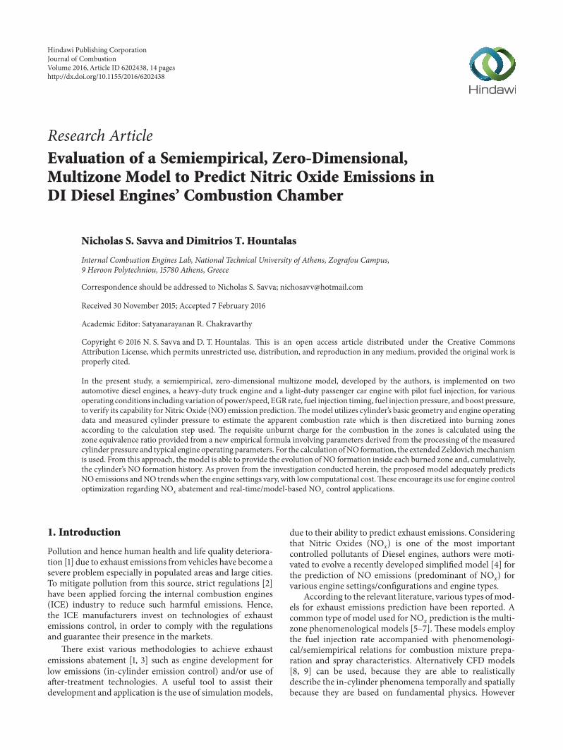
The model’s concept is described schematically in Fig-ure 1. Each filled symbol corresponds to the generation of acombustion zone. The fuel attributed to each zone is derivedfrom the discretization of combustion rate according to thecrank angle (CA) calculation step. The unburnt charge mass(air + EGR + RG) amount used at the zone generationis determined from the zone equivalence ratio (Φ) andthe corresponding zone fuel amount. Complete/homogenousmixing of the fuel and unburnt charge is assumed. Bythis approach, the employment of spray models (e.g., phe-nomenological multizone) or/and space geometrical dis-cretization (e.g., mesh) is avoided. After their generation, thecombustion zones are being compressed/expanded (emptysquares in Figure 1), according to the pressure derivative,inside the cylinder until EVO. The zones are autonomousand do not exchange mass and heat between them. NO isformed inside each zone from its generation up to EVO byusing the extended Zeldovich mechanism. Via this concept,the evolution of zone NO formation inside the cylinder,during an engine cycle, is provided.The cumulative NO fromthe zones at each calculation CA step provides the overallevolution of NO formation as shown in Figure 2.

3. Basic Calculations

3.1. Initial Conditions. The initial conditions required fromthe model are the in-cylinder trapped mass (unburnt charge)

Journal of Combustion 3

EOCSOC

EOC

EVO

Figure 1: The multizone approach for the NO calculation [4].

160 180 200 220 240 260 280 300 320 3400.0

0.5

1.0

1.5

2.0

2.5

NO

(km

ol)

0

0.1

0.2

0.3

Inst

anta

neou

s bur

nt fu

el m

ass (

mg)

0

20

40

60

80

100

In-c

ylin

der p

ress

ure (

bar)

NO formationhistory

p

MFB

EVO

Tailpipe NO

×10−8

Crank angle (∘ABDC)

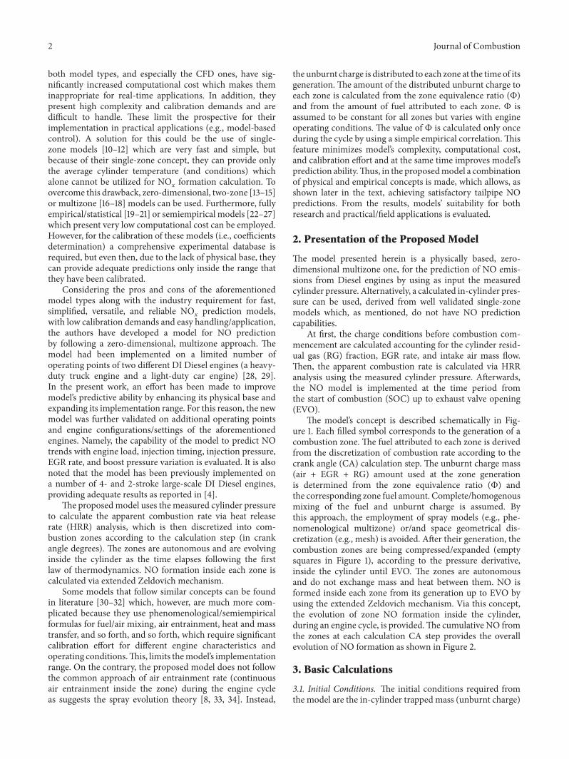
Figure 2: NO formation history inside the combustion chamberduring an engine cycle alongwith cylinder pressure and fuel amountburnt at each CA step.

and its composition and temperature at combustion com-mencement. The trapped mass (��tr [g/cycle]) is assumedto be unchanged from intake valve closure (IVC) up toSOC-1. Its composition is considered constant throughoutthe cycle assuming no interaction between the zones. Thetrapping efficiency is assumed to be equal to unity (realisticfor 4-stroke engines) [34] and thus the trapped mass iscalculated from (1) by using the following inputs: number ofcylinders (𝑛cyl), engine speed (𝑁 [rpm]), intake air mass flow(��IA [kg/h]), and EGR and RG mass fractions:

��tr =��IA ⋅ 100/3

𝑛cyl ⋅ 𝑁⋅

1 + RG1 − EGR

. (1)

In the presentwork, the experimental data for ��IA , EGR rate,and RG fraction were supplied from external provider. Here,it is noted that the values of ��IA and EGR rate (EGR valve

position) can be reliably measured “on-board” in real-timeand RG fraction can be estimated using simplified models.Furthermore, these parameters can be obtained from theECU since they can be mapped as functions of engine speedand load. Alternatively, ��IA could be estimated directly usingthe measured pressure and temperature at intake manifoldand the cylinder pressure, via a simplified zero-dimensionalmodel [35, 36], or indirectly from the exhaust gas oxygencontent.

The composition of EGR and RG gases is assumed to beidentical to the one of the exhaust gas which is calculatedby assuming ideal combustion using the global Φ andaccounting for the fuel composition (H/C). The compositionof the unburnt charge is calculated using the EGR, RG,and ambient air mass fractions and compositions. Using thetrappedmass, its composition (molecular weight (MW)), andthe corresponding cylinder pressure and volume via the idealgas state equation, the unburnt charge temperature at SOC-1 is provided. This temperature serves as the initial value forthe calculation of unburnt zone temperature.

3.2. Utilizing the Measured Cylinder Pressure and HRR. Theprocesses evolving inside the engine cylinder are directlyor implicitly reflected on the measured cylinder pressure[34]. From these processes that involve compression, fuel-air mixing, combustion, expansion, and so forth, the ther-modynamic condition of the charge, which affects NOxformation mechanism, is determined. Moreover, the effect ofheat transfer, leakages, inlet conditions, turbulence, fuel-airmixing, engine geometry, and so forth on these mechanismsis also implicitly accounted for when the actual cylinderpressure is used. Furthermore, the effect of injection strategy(pilot/post, multiple injection) is implicitly accounted forbecause the actual cylinder pressure and combustion rate (i.e.,HRR) are used. Thus, the use of measured cylinder pressureadds versatility to the model since the variations occurringinside the cylinder, and having an effect on NO formation,can be captured.

As mentioned, the combustion rate (i.e., fuel amount(𝑚𝑓) combusted at each time (CA) step; e.g., see Figure 2)is calculated directly from HRR, assuming instantaneouscombustion, as shown in (2) (𝑑𝑝 is derived from the mea-sured cylinder pressure), by dividing the gross heat release(𝑑𝑄gross [J]) by the fuel lower heating value (LHV [J/kg]) asdescribed in (3):

𝑑𝑄gross

𝑑CA=

𝑑𝐻sens𝑑CA

− 𝑉 ⋅𝑑𝑝

𝑑CA+

𝑑𝑄𝑤

𝑑CA, (2)

𝑚𝑓 =

𝑑𝑄gross/𝑑CA ⋅ ΔCALHV

. (3)

For the heat exchange (𝑑𝑄𝑤/𝑑CA [J/∘CA]) through thecylinder wall, the Annand formula has been used [34, 37] dueto the less computational cost and calibration effort requiredcompared to theWoschni [38]model. Detailed description ofthe HRR calculations is presented in [4].


3.3. Unburnt Zone Evolution inside the Cylinder. The chem-ical composition of the unburnt zone is assumed to be con-stant for the entire closed cycle; namely, it does not interactwith the combustion zones. When combustion commences,the requisite unburnt charge amount for the combustionduring zone formation is obtained from the unburnt zone.Thus the unburnt zone mass is consumed as combustionpersists. The volume (𝑉ub [m

3]) of the unburnt zone at each

calculation step is calculated by subtracting the volumes ofthe existing combustion zones from the current cylindervolume. Its temperature, which corresponds to reactants’temperature during combustion at zone generation, is calcu-lated by using the first law of thermodynamics at eachCA step(𝑖) following an iterative procedure. This procedure involves(4) for the enthalpy calculation and (5) (Newton-Raphson[39] method) for the temperature calculation:

ℎ𝑘𝑖 =

𝑛𝑖−1 ⋅ ℎ𝑖−1 + 𝑑𝑝𝑖 ⋅ (𝑉𝑖−1 + 𝑉𝑖) /2 − 𝑛out ⋅ (ℎ𝑖−1 + ℎ𝑘−1𝑖 ) /2 − 𝑑𝑄𝑤

𝑘𝑖

𝑛𝑖

, 𝑛𝑖 = 𝑛𝑖−1 − 𝑛out, (4)

𝑇𝑘𝑖 = 𝑇

𝑘−1𝑖 −

ℎ𝑘𝑖 − ℎ𝑘−1𝑖

𝑐𝑝𝑘−1𝑖

. (5)

In the previous expressions 𝑛 [kmol] is the number ofmoles comprised in the unburnt zone and is calculated bysubtracting from the number of moles of the previous CAstep the moles required from the zone (𝑛out [kmol]), whichis generated at the current CA step. Furthermore, 𝑑𝑄𝑤 [J]corresponds to the heat transfer through the cylinder wallcalculated using Annand’s model [37] where the current in-cylinder area is multiplied by 𝑉

𝑘ub,𝑖/𝑉cyl𝑖 to fairly represent

the equivalent zone area. Superscript 𝑘 denotes the iterationsequence number. Detailed description of the heat transferthrough the cylinder wall method used can be found in [4].

3.4. Generation and Evolution of the Combustion Zones. Inorder to consider convincingly the local conditions (i.e.,temperature, species concentration) inside the combustionchamber, which determine the NO formation [34, 40, 41], amultizone approach is adopted (see Figure 1).

The mass of each zone (𝑚 [kg]), after its generation,remains constant throughout the cycle since the zones donot interact. The pressure inside the zones coincides withthe measured cylinder pressure. Zone temperature (𝑇𝑝 [K])is determined by the use of the first law of thermodynamicsvia a Newton-Raphson [39] iterative methodology describedin

𝑇𝑝𝑘𝑧,𝑖 = 𝑇𝑝

𝑘−1𝑧,𝑖

−ℎ𝑝𝑘−1𝑧,𝑖 − ℎ𝑟𝑧,𝑖 + 𝑑𝑞𝑤

𝑘−1𝑧,𝑖 − 𝑉

𝑘−1𝑧,𝑖 ⋅ 𝑑𝑝𝑖/𝑚𝑧

𝑐𝑝𝑘−1𝑧,𝑖

.

(6)

Zone composition is derived from the combustion of the fueland the corresponding unburnt charge, accounting for chem-ical dissociation (see Section 3.5) of combustion products.For the calculation of enthalpy before combustion (ℎ𝑟 [J/kg]),the reactants’ temperature (𝑇𝑟 [K]) and composition are used,which are equal to the ones of the unburnt charge at theexamined CA step (see Section 3.3). On the other hand,enthalpy after combustion (ℎ𝑝 [J/kg]) is a function of 𝑇𝑝 andcombustion products composition. Zone volume (𝑉 [m3])

is calculated via the ideal gas state equation. 𝑑𝑞𝑤 [J/kg]corresponds to the heat transfer between the zone andcylinder wall and is calculated using Annand’s model [37]similarly to the unburnt zone calculation (see Section 3.3).

After its formation, the zone evolves throughout the closeengine cycle following the first law of thermodynamics andaccording to the cylinder pressure evolution. Therefore, ateach CA step (𝑖), the values of volume, composition, enthalpy,and temperature of the examined zone (𝑧) are calculatediteratively.The enthalpy (ℎ) and temperature (𝑇) of each zone(𝑧) are calculated from the following equations, respectively:

ℎ𝑘𝑧,𝑖 =

𝑛𝑧,𝑖−1 ⋅ ℎ𝑧,𝑖−1 + 𝑑𝑝𝑖 ⋅ (𝑉𝑧,𝑖−1 + 𝑉𝑘𝑧,𝑖) /2 − 𝑑𝑄𝑤

𝑘𝑧,𝑖

𝑚𝑧/MW𝑘𝑧,𝑖, (7)

𝑇𝑘𝑧,𝑖 = 𝑇

𝑘−1𝑧,𝑖 −

ℎ𝑘𝑧,𝑖 − ℎ

𝑘−1𝑧,𝑖

𝑐𝑝𝑘−1𝑧,𝑖

. (8)

Apparently, the initiation values for the iteration at each CAstep equal the respective final ones of the previous step.When the zone temperature (𝑇) converges, the calculationprocedure proceeds to the next CA step.

3.5. Chemical Dissociation Mechanism. The calculation ofzone temperature accounts for the combustion productsdissociation.This mechanism results in a noticeable decreaseof combustion temperature since most of its reactions areendothermic. Furthermore, for the zone equilibrium compo-sition calculation, the proposed model uses a chemical dis-sociation scheme [42–44], which involves 11 chemical species(O2 for fuel lean or C12H26 for fuel rich, N2, CO2, H2O,H,H2,N,NO,O,OH,CO), seven equilibrium reactions, and the fourconservation equations describing the combustion for theC/H/O/N system. Equilibrium composition is utilized duringthe NO formation calculation described next. Equilibriumconstants are derived from minimization of the Gibbs freeenergy of the chemical reactions used. This scheme has beendescribed in detail in previous publications [4, 28, 29] of theauthors.


3.6. Calculation of Nitric Oxide Formation. In the presentstudy only the thermal NOx formation mechanism is consid-ered (i.e., NO formation), since this mechanism is predom-inant at high-temperature, stoichiometric diffusion flamewhich characterizes DI Diesel combustion [34, 40, 45].

Due to the higher time required for NO formationcompared to the time available for combustion processesinside the combustion chamber of DI Diesel engines, NOrarely reaches equilibrium. Hence, NO formation is kineti-cally controlled [34, 41] while equilibrium concentration isassumed for the remaining species. Therefore, the extendedZeldovich mechanism [34, 40, 46, 47] has been used, whichis described from the three reactions shown in

O + N2𝑅1

←→ NO + N

N + O2𝑅2

←→ NO + O

N + OH𝑅3

←→ NO + H

(9)

Their reaction rate constants, which are functions oftemperature and used for the reaction rates calculation(𝑅1,2,3 [kmol/m3/s]), are derived from [48].

NO formation rate is calculated from (10), which isderived from the mathematical processing [40, 41] of the dif-ferential equations that describe the kinetics of the extendedZeldovich mechanism:

(𝑑NO𝑑CA

)

𝑧,𝑖

= (𝑑 [NO]

𝑑𝑡)

𝑧,𝑖

⋅ 𝑉𝑧,𝑖 ⋅𝑑𝑡

𝑑CA

=

2 ⋅ 𝑅1 ⋅ {1 − ([NO] / [NO]𝑒)2}

1 + ([NO] / [NO]𝑒) ⋅ 𝑅1/ (𝑅2 + 𝑅3)

⋅𝑉𝑧,𝑖

6 ⋅ 𝑁.

(10)

In the previous expression,𝑉𝑧,𝑖 [m3] is the zone (𝑧) volume at

the examined CA step (𝑖). The integration of (10) in the CAdomain until EVO provides the NO [Kmol] amount formedinside each zone and cumulatively inside the cylinder, at eachCA step.

Comprehensive description of the model can be found in[4]. In the present work, an improved correlation for zoneequivalence ratioΦ is introduced, as presented next, in orderto enhance model’s NO prediction capability.

3.7. Calculation of Zone Equivalence Ratio Φ. According tothe model’s rationale (see Section 2), the total mass of eachzone is determined from the mass of the combusted fuel atthe time of its generation and the requisite unburnt chargemass. The latest is determined from the corresponding zonefuelmass and the zone equivalence ratio (Φ). Alongwith zonemass, the value of Φ also affects zone volume, temperature,and chemical composition which in turn affect significantlythe NO formation mechanism.

For NO formation, a constant value of Φ is used which isidentical for all zones, instead of using a phenomenological

0.6 0.7 0.8 0.9 1 1.1 1.2

0

1

2

3

4

5

6Passengercar engine

Truckengine

Calculated NO =Measured NO

Theoretical zone equivalence ratio (Φz)

NO

calc

ulat

ed/N

Om

easu

red

Figure 3: Variation of calculated/measured NO ratio with zoneequivalent ratio Φ.

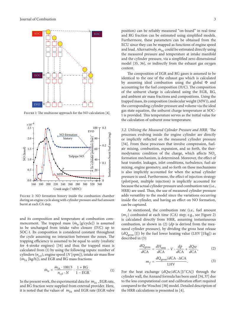
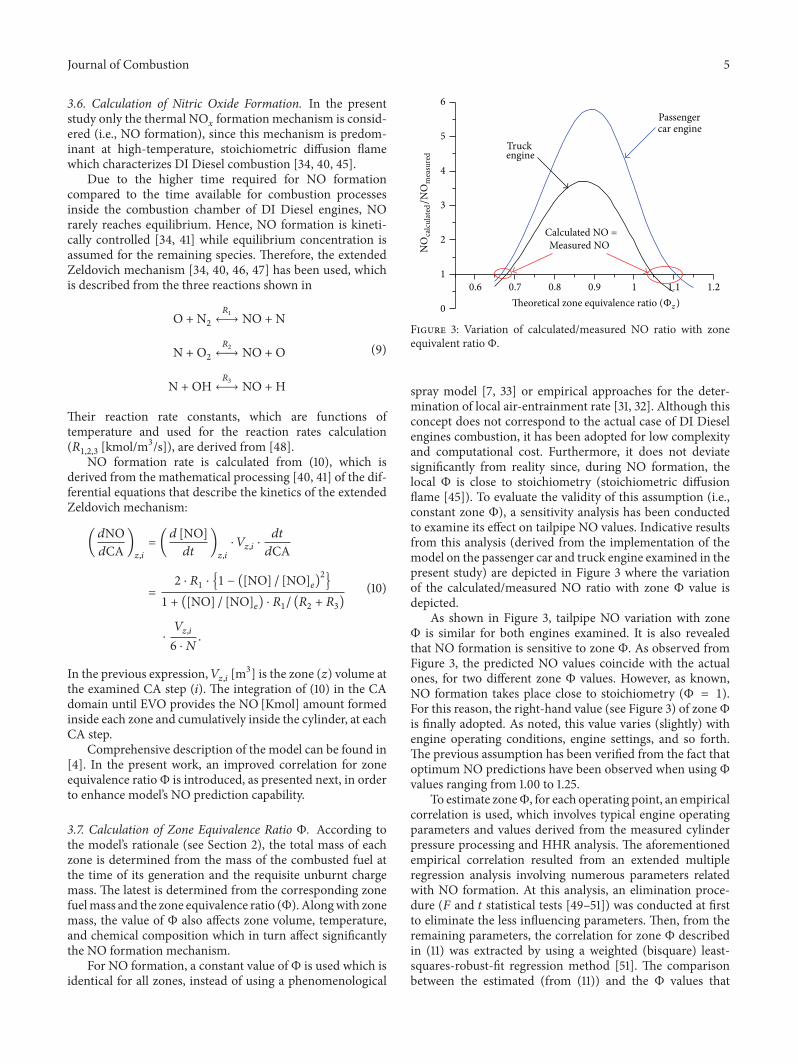
spray model [7, 33] or empirical approaches for the deter-mination of local air-entrainment rate [31, 32]. Although thisconcept does not correspond to the actual case of DI Dieselengines combustion, it has been adopted for low complexityand computational cost. Furthermore, it does not deviatesignificantly from reality since, during NO formation, thelocal Φ is close to stoichiometry (stoichiometric diffusionflame [45]). To evaluate the validity of this assumption (i.e.,constant zone Φ), a sensitivity analysis has been conductedto examine its effect on tailpipe NO values. Indicative resultsfrom this analysis (derived from the implementation of themodel on the passenger car and truck engine examined in thepresent study) are depicted in Figure 3 where the variationof the calculated/measured NO ratio with zone Φ value isdepicted.

As shown in Figure 3, tailpipe NO variation with zoneΦ is similar for both engines examined. It is also revealedthat NO formation is sensitive to zone Φ. As observed fromFigure 3, the predicted NO values coincide with the actualones, for two different zone Φ values. However, as known,NO formation takes place close to stoichiometry (Φ = 1).For this reason, the right-hand value (see Figure 3) of zoneΦ

is finally adopted. As noted, this value varies (slightly) withengine operating conditions, engine settings, and so forth.The previous assumption has been verified from the fact thatoptimum NO predictions have been observed when using Φ

values ranging from 1.00 to 1.25.To estimate zoneΦ, for each operating point, an empirical

correlation is used, which involves typical engine operatingparameters and values derived from the measured cylinderpressure processing and HHR analysis. The aforementionedempirical correlation resulted from an extended multipleregression analysis involving numerous parameters relatedwith NO formation. At this analysis, an elimination proce-dure (𝐹 and 𝑡 statistical tests [49–51]) was conducted at firstto eliminate the less influencing parameters. Then, from theremaining parameters, the correlation for zone Φ describedin (11) was extracted by using a weighted (bisquare) least-squares-robust-fit regression method [51]. The comparisonbetween the estimated (from (11)) and the Φ values that


Table 1: Engine data.

Engine A Engine BNumber of cylinders 6 4Bore [mm] 102 88Stroke [mm] 130 88.4Connecting rod length [mm] 215 149Compression ratio 18.5 18.0Displacement volume [lt] 6.37 2.15

Maximum brake power output 205 kW@2300 rpm

92 kW@4200 rpm

Inlet valve close [∘CA ATDC] −171 −123Exhaust valve open [∘CAATDC] 121 135

provide matching between experimental and calculated NOvalues (see Figure 3) presents an RMSE = 1.47%:

Φ = 𝑐0 + 𝑐1 ⋅ (𝑝IVC𝑝amb

)

−1

+ 𝑐2 ⋅ (𝑝SOCmain

𝑝amb)

−1

+ 𝑐3

⋅𝑝comb. max𝑝SOCmain

+ 𝑐4 ⋅COCTDC

+ 𝑐5 ⋅ Φeng. overall + 𝑐6

⋅

𝑆𝑝

𝑆𝑝ref+ 𝑐7 ⋅

𝑃

𝑃ref.

(11)

In the previous expression SOCmain corresponds to theCA [∘CA ABDC] (BDC ≡ 0∘CA) of the main combustioncommencement, TDC (≡180∘CA ABDC) to top dead center,COC to center of combustion, and IVC to intake valveclosure;𝑃 and 𝑆𝑝 are the engine brake power output [kW] andmean piston speed [m/s], respectively. The reference 𝑃 (𝑃ref)corresponds to themaximumengine brake power output (seeTable 1) and the reference 𝑆𝑝 (𝑆𝑝ref ) equals 10 [m/s].

The first parameter (𝑝IVC/𝑝amb) of (11) accounts for theeffect of intake air pressure, while the second (𝑝SOCmain

/𝑝amb)accounts for the effect of compression ratio. The thirdone (𝑝comb. max/𝑝SOCmain

) accounts for the effect of pres-sure derivative (pressure increase due to combustion whichstrongly affects NO formation) which is also related with SOI.The fourth parameter (COC/TDC) accounts for the effectof combustion duration. The fifth parameter (Φeng. overall)provides information for the overall air supply while the sixth(𝑆𝑝/𝑆𝑝ref ) accounts for the effect of engine speed on fuel-air mixing and available time for NO formation. Finally, theseventh parameter (𝑃/𝑃ref ) accounts for the effect of engineload.

4. Test Engine Description

The present model is implemented on a heavy-duty truckengine (Engine A) and a light-duty passenger car engine(Engine B) to test its ability to predict NO emissions. Bothengines are supercharged Diesels, equipped with a common-rail DI fuel injection system and a high pressure EGR system

using EGR cooler. The defenses between the two testedengines are the following:

(1) In contrast with the truck engine, the passenger carengine uses pilot fuel injection, mainly to reduceengine noise.

(2) The truck engine has two additional cylinders andtreble displacement volume compared to the carengine.

(3) Since the examined engines are designed for differentoperating areas, they have different fuel injectionstrategy (i.e., injection profile, timing, etc.) and valvetiming. Furthermore, due to the high torque demandof the truck engine, it produces higher power outputand operates at lower engine speeds.

The main data of the test engines are summarized in Table 1.

5. Test Cases Examined

In the present work, numerous measurements were used toevaluate the ability of the proposed model to predict NOemissions. The experimental measurements were providedby AVL and ETH during cooperation under an EU fundedproject. It is emphasized that the provided experimentalmeasurements were tailpipe NO concentrations (measuredusing chemiluminescence analyzers able to provide bothmeasurements: NO and total NOx) which, as mentioned (seeSection 3.6), is usually the predominant of NOx regardingDiesel engines.

The examined operating points for Engine A are catego-rized as follows:

(1) Operating points corresponding to the ExtendedEuropean Stationary Cycle (EESC). The EESCincludes seven load points for five engine speed cases(1400–2200 rpm), namely, 35 operating points.As for the mid-speed and mid-load engine operation(1800 rpm and 86 kW) the following cases are exam-ined:

(2) SOI variation from −20 to +10∘CA ATDC.(3) EGR rate variation from 2 to 18%.(4) Fuel injection pressure (rail pressure) variation from

1000 to 1400 bar.(5) Inlet manifold pressure variation from 1.3 to 2 bar

(abs.).

For Engine B, the following parameters are varied, consid-ering three operating points, namely, 2000 rpm and 29.4 kW,2500 rpm and 18.3 kW, and 2500 rpm and 31.4 kW:

(1) EGR rate from 0 to 25%.(2) Fuel injection pressure from 500 to 1000 bar.(3) SOI from −10 to 6∘CA ATDC.(4) Inlet manifold pressure from 1.1 to 1.7 bar (abs.)

Thus a total of 132 operating points were examined, 60 ofwhich are attributed to Engine A and 72 to Engine B.


6. Results and Discussion

6.1. Heavy-Duty Truck Engine (Engine A)

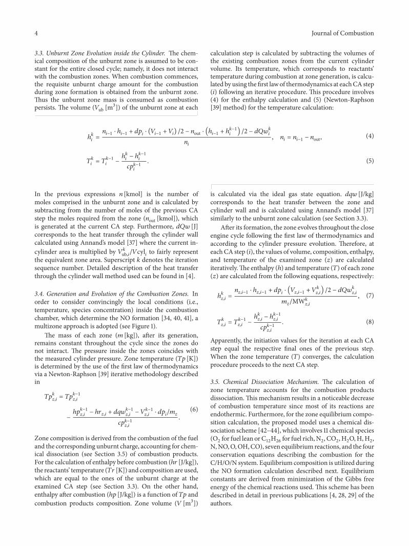
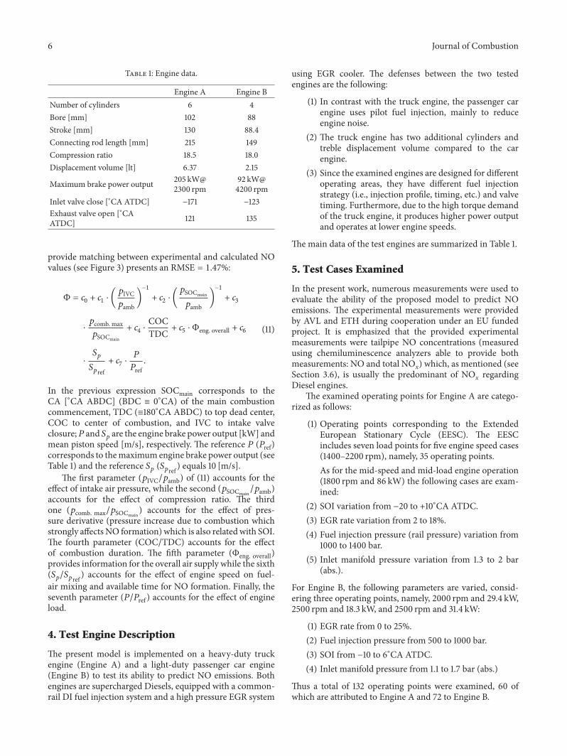
6.1.1. Prediction of NO at the EESC Operating Points. Initiallythe model was implemented on Engine A, for various oper-ating points corresponding to the EESC, to predict NO emis-sions. The operating points of this cycle are defined by theengine load and speed.The SOI, EGR, fuel injection pressure,and intake manifold pressure settings were obtained fromthe ECU (default settings).The comparison of calculated andmeasured NO values against engine power for various speedsis presented in Figure 4.

As revealed from the observation of Figure 4, the pro-posed model is able to predict satisfactorily the NO trendwith engine power. The trend is approximately linear anddecreases with engine speed. A higher difference betweencalculated andmeasured absolute values for the highest loadscan be also observed. This is mostly attributed to the highestin-cylinder pressure signal noise during expansion phase.Theresult is combustion duration overestimation and high heatrelease peeks causing increased NO formation.

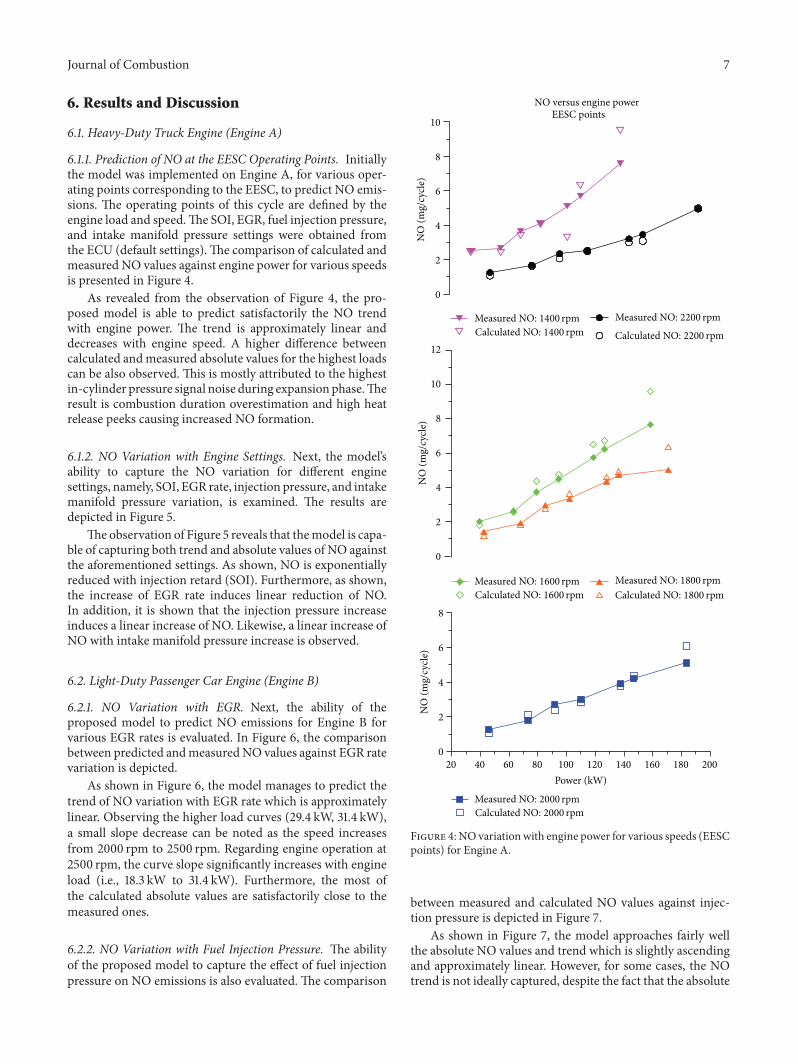
6.1.2. NO Variation with Engine Settings. Next, the model’sability to capture the NO variation for different enginesettings, namely, SOI, EGR rate, injection pressure, and intakemanifold pressure variation, is examined. The results aredepicted in Figure 5.

The observation of Figure 5 reveals that themodel is capa-ble of capturing both trend and absolute values of NO againstthe aforementioned settings. As shown, NO is exponentiallyreduced with injection retard (SOI). Furthermore, as shown,the increase of EGR rate induces linear reduction of NO.In addition, it is shown that the injection pressure increaseinduces a linear increase of NO. Likewise, a linear increase ofNO with intake manifold pressure increase is observed.

6.2. Light-Duty Passenger Car Engine (Engine B)

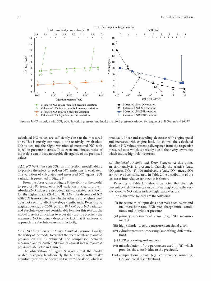
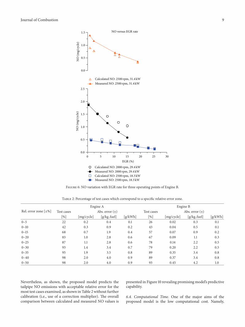
6.2.1. NO Variation with EGR. Next, the ability of theproposed model to predict NO emissions for Engine B forvarious EGR rates is evaluated. In Figure 6, the comparisonbetween predicted andmeasuredNO values against EGR ratevariation is depicted.

As shown in Figure 6, the model manages to predict thetrend of NO variation with EGR rate which is approximatelylinear. Observing the higher load curves (29.4 kW, 31.4 kW),a small slope decrease can be noted as the speed increasesfrom 2000 rpm to 2500 rpm. Regarding engine operation at2500 rpm, the curve slope significantly increases with engineload (i.e., 18.3 kW to 31.4 kW). Furthermore, the most ofthe calculated absolute values are satisfactorily close to themeasured ones.

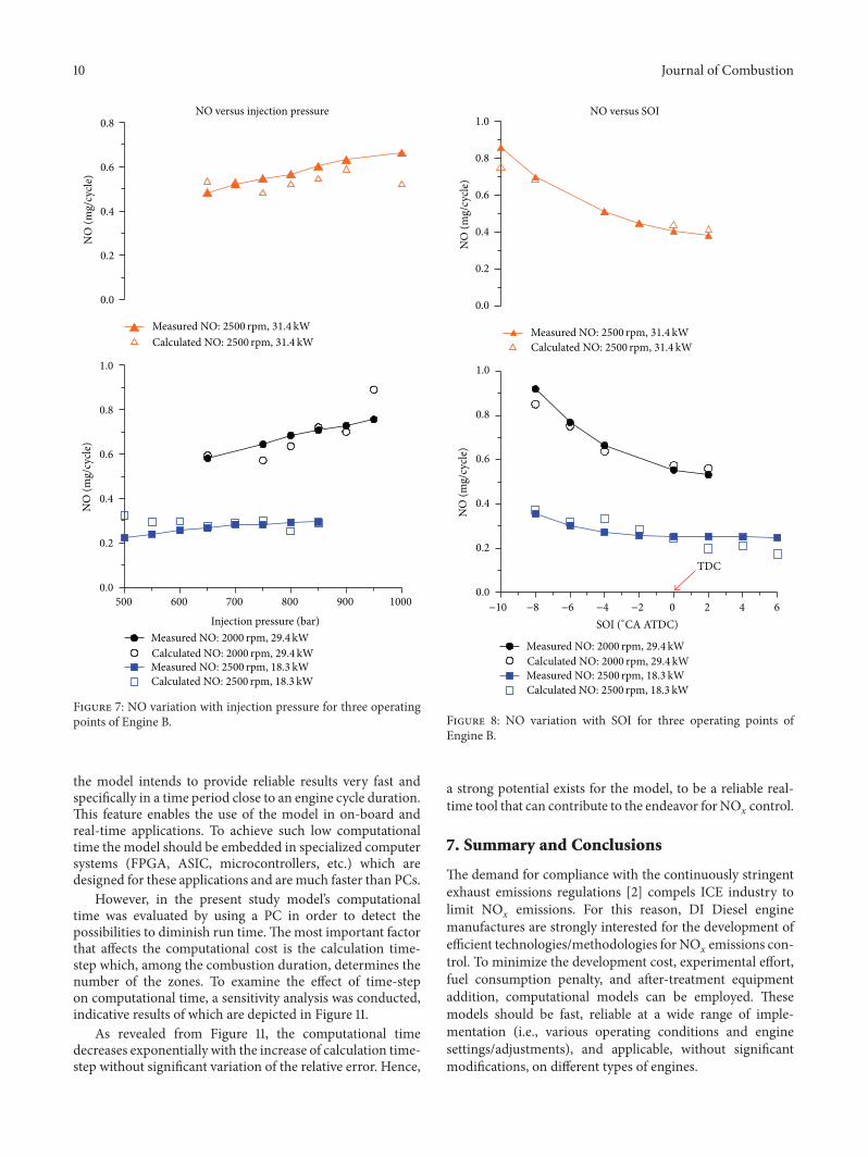
6.2.2. NO Variation with Fuel Injection Pressure. The abilityof the proposed model to capture the effect of fuel injectionpressure on NO emissions is also evaluated. The comparison

20 40 60 80 100 120 140 160 180 200Power (kW)

0

2

4

6

8

0

2

4

6

8

10

12

NO

(mg/

cycle

)N

O (m

g/cy

cle)

NO

(mg/

cycle

)

0

2

4

6

8

10

NO versus engine powerEESC points

Measured NO: 1400 rpmCalculated NO: 1400 rpm

Measured NO: 2200 rpm

Calculated NO: 2200 rpm




Figure 4: NO variationwith engine power for various speeds (EESCpoints) for Engine A.

between measured and calculated NO values against injec-tion pressure is depicted in Figure 7.

As shown in Figure 7, the model approaches fairly wellthe absolute NO values and trend which is slightly ascendingand approximately linear. However, for some cases, the NOtrend is not ideally captured, despite the fact that the absolute


−20 −15 −10 −5 0 5 10

2 4 6 8 10 12 14 16 18EGR (%)

1000 1100 1200 1300 1400

1.3 1.4 1.5 1.6 1.7 1.8 1.9 2

0

2

4

6

8

10

12

14

16

18

0

2

4

6

8

10

12

14

16

18

NO versus engine settings variation

Measured NO: SOI variationCalculated NO: SOI variationMeasured NO: EGR variationCalculated NO: EGR variation

Measured NO: intake manifold pressure variationCalculated NO: intake manifold pressure variationMeasured NO: injection pressure variationCalculated NO: injection pressure variation

TDC

NO

(mg/

cycle

)

NO

(mg/

cycle

)

Intake manifold pressure (bar (abs.))

Injection pressure (bar) SOI (∘CA ATDC)

Figure 5: NO variation with SOI, EGR, injection pressure, and intake manifold pressure variation for Engine A at 1800 rpm and 86 kW.

calculated NO values are sufficiently close to the measuredones. This is mostly attributed to the relatively low absoluteNO values and the slight variation of measured NO withinjection pressure increase. Thus, even small inaccuracies ofinput data can induce noticeable divergence of the predictedvalues.

6.2.3. NO Variation with SOI. In this section, model’s abilityto predict the effect of SOI on NO emissions is evaluated.The variation of calculated and measured NO against SOIvariation is presented in Figure 8.

From the observation of Figure 8, the ability of the modelto predict NO trend with SOI variation is clearly proven.Absolute NO values are also adequately calculated. As shown,for the higher loads (29.4 and 31.4 kW) the decrease of NOwith SOI is more intensive. On the other hand, engine speeddoes not seem to affect the slope significantly. Referring toengine operation at 2500 rpm and 18.3 kW, bothNO variationand absolute values are considerably low. For this reason, themodel presents difficulties to accurately capture precisely themeasured NO tendency despite the fact that it achieves toapproach the absolute values satisfactorily.

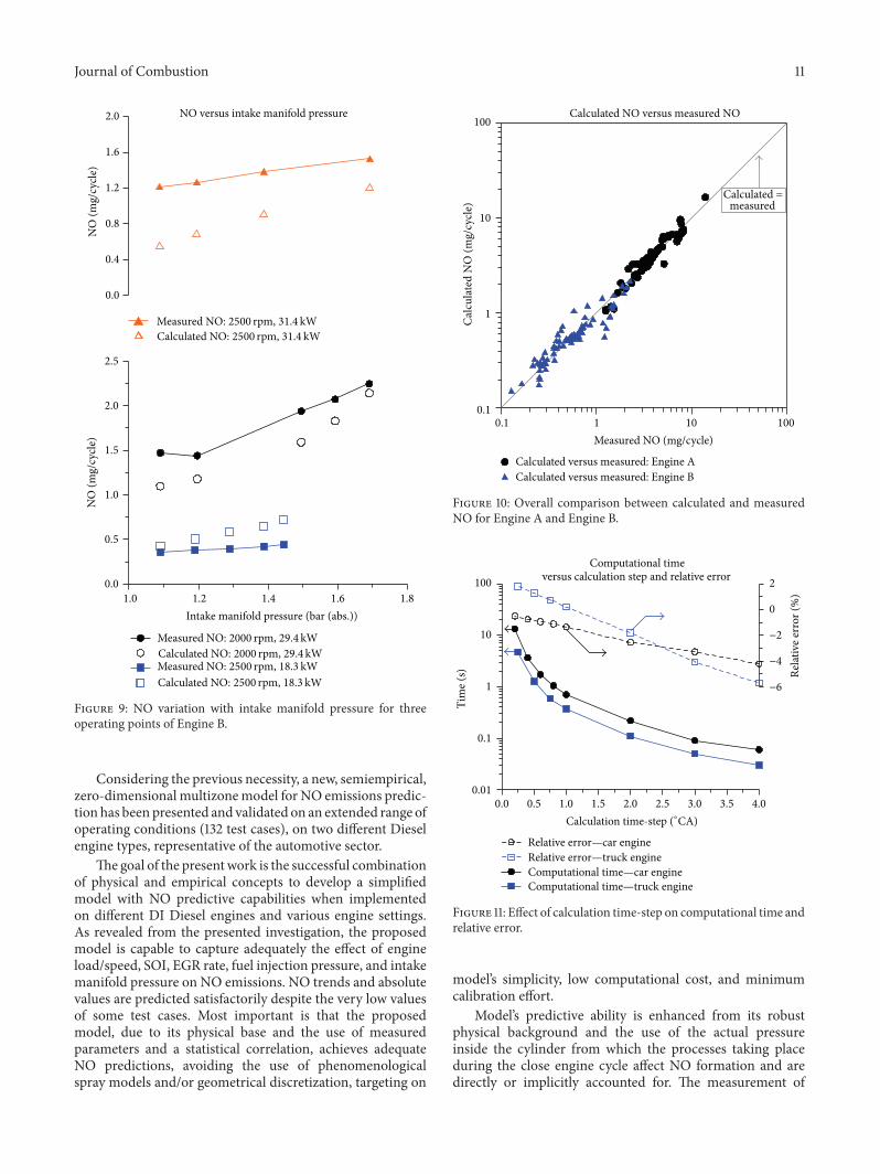
6.2.4. NO Variation with Intake Manifold Pressure. Finally,the ability of themodel to predict the effect of intakemanifoldpressure on NO is evaluated. The comparison betweenmeasured and calculated NO values against intake manifoldpressure is depicted in Figure 9.

The observation of Figure 9 reveals that the modelis able to approach adequately the NO trend with intakemanifold pressure. As shown in Figure 9, the slope, which is

practically linear and ascending, decreases with engine speedand increases with engine load. As shown, the calculatedabsolute NO values present a divergence from the respectivemeasured ones which is possibly due to their very low valueswhich induce high relative errors.

6.3. Statistical Analysis and Error Sources. At this point,an error analysis is presented. Namely, the relative (calc.NOx/meas. NOx− 1) ⋅ 100 and absolute (calc. NO−meas. NO)errors have been calculated. In Table 2 the distribution of thetest cases into relative error zones is shown.

Referring to Table 2, it should be noted that the highpercentage (relative) error can bemisleading because the verylow absolute NO values induce high relative errors.

The main error sources are the following:

(i) inaccuracies of input data (normal) such as air andfuel mass flow rate, EGR rate, charge initial condi-tions, and in-cylinder pressure,

(ii) primary measurement error (e.g., NO measure-ments),

(iii) high cylinder pressure measurement signal error,(iv) cylinder pressure processing (smoothing, differentia-

tion),(v) HRR processing and analysis,(vi) miscalculation of the parameters used in (11) which

provides the zone Φ (due to the previous),(vii) computational errors (e.g., convergence, rounding,

CA, and zonal discretization).


0 5 10 15 20 25 30EGR (%)

0.0

0.5

1.0

1.5

2.0

2.5

0.0

0.5

1.0

1.5 NO versus EGR rate

NO

(mg/

cycle

)N

O (m

g/cy

cle)

Calculated NO: 2500 rpm, 31.4 kWMeasured NO: 2500 rpm, 31.4 kW

Calculated NO: 2000 rpm, 29.4 kWMeasured NO: 2000 rpm, 29.4 kWCalculated NO: 2500 rpm, 18.3 kWMeasured NO: 2500 rpm, 18.3 kW

Figure 6: NO variation with EGR rate for three operating points of Engine B.

Table 2: Percentage of test cases which correspond to a specific relative error zone.

Rel. error zone [±%]Engine A Engine B

Test cases Abs. error (±) Test cases Abs. error (±)[%] [mg/cycle] [g/kg fuel] [g/kWh] [%] [mg/cycle] [g/kg fuel] [g/kWh]

0–5 22 0.2 0.4 0.1 26 0.02 0.3 0.10–10 42 0.3 0.9 0.2 43 0.04 0.5 0.10–15 68 0.7 1.9 0.4 57 0.07 0.9 0.20–20 83 1.0 2.8 0.6 67 0.09 1.1 0.30–25 87 1.1 2.8 0.6 78 0.14 2.2 0.50–30 93 1.4 3.4 0.7 79 0.20 2.2 0.50–35 95 1.9 3.5 0.8 89 0.35 3.4 0.80–40 98 2.0 4.0 0.9 89 0.37 3.4 0.80–50 98 2.0 4.0 0.9 93 0.45 4.2 1.0

Nevertheless, as shown, the proposed model predicts thetailpipe NO emissions with acceptable relative error for themost test cases examined, as shown in Table 2 without furthercalibration (i.e., use of a correction multiplier). The overallcomparison between calculated and measured NO values is

presented in Figure 10 revealing promisingmodel’s predictivecapability.

6.4. Computational Time. One of the major aims of theproposed model is the low computational cost. Namely,


500 600 700 800 900 1000

Injection pressure (bar)

0.0

0.2

0.4

0.6

0.8

1.0

0.0

0.2

0.4

0.6

0.8NO versus injection pressure

NO

(mg/

cycle

)N

O (m

g/cy

cle)

Calculated NO: 2000 rpm, 29.4kWMeasured NO: 2000 rpm, 29.4 kW



Figure 7: NO variation with injection pressure for three operatingpoints of Engine B.

the model intends to provide reliable results very fast andspecifically in a time period close to an engine cycle duration.This feature enables the use of the model in on-board andreal-time applications. To achieve such low computationaltime the model should be embedded in specialized computersystems (FPGA, ASIC, microcontrollers, etc.) which aredesigned for these applications and are much faster than PCs.

However, in the present study model’s computationaltime was evaluated by using a PC in order to detect thepossibilities to diminish run time.Themost important factorthat affects the computational cost is the calculation time-step which, among the combustion duration, determines thenumber of the zones. To examine the effect of time-stepon computational time, a sensitivity analysis was conducted,indicative results of which are depicted in Figure 11.

As revealed from Figure 11, the computational timedecreases exponentially with the increase of calculation time-step without significant variation of the relative error. Hence,

−10 −8 −6 −4 −2 0 2 4 60.0

0.2

0.4

0.6

0.8

1.0

0.0

0.2

0.4

0.6

0.8

1.0NO versus SOI

TDC

NO

(mg/

cycle

)N

O (m

g/cy

cle)

SOI (∘CA ATDC)

Calculated NO: 2000 rpm, 29.4kWMeasured NO: 2000 rpm, 29.4kW



Figure 8: NO variation with SOI for three operating points ofEngine B.

a strong potential exists for the model, to be a reliable real-time tool that can contribute to the endeavor forNOx control.

7. Summary and Conclusions

The demand for compliance with the continuously stringentexhaust emissions regulations [2] compels ICE industry tolimit NOx emissions. For this reason, DI Diesel enginemanufactures are strongly interested for the development ofefficient technologies/methodologies for NOx emissions con-trol. To minimize the development cost, experimental effort,fuel consumption penalty, and after-treatment equipmentaddition, computational models can be employed. Thesemodels should be fast, reliable at a wide range of imple-mentation (i.e., various operating conditions and enginesettings/adjustments), and applicable, without significantmodifications, on different types of engines.


1.0 1.2 1.4 1.6 1.8Intake manifold pressure (bar (abs.))

0.0

0.4

0.8

1.2

1.6

2.0

0.0

0.5

1.0

1.5

2.0

2.5

NO versus intake manifold pressure

NO

(mg/

cycle

)N

O (m

g/cy

cle)

Calculated NO: 2000 rpm, 29.4 kWMeasured NO: 2000 rpm, 29.4kW



Figure 9: NO variation with intake manifold pressure for threeoperating points of Engine B.

Considering the previous necessity, a new, semiempirical,zero-dimensional multizonemodel for NO emissions predic-tion has beenpresented and validated on an extended range ofoperating conditions (132 test cases), on two different Dieselengine types, representative of the automotive sector.

The goal of the presentwork is the successful combinationof physical and empirical concepts to develop a simplifiedmodel with NO predictive capabilities when implementedon different DI Diesel engines and various engine settings.As revealed from the presented investigation, the proposedmodel is capable to capture adequately the effect of engineload/speed, SOI, EGR rate, fuel injection pressure, and intakemanifold pressure on NO emissions. NO trends and absolutevalues are predicted satisfactorily despite the very low valuesof some test cases. Most important is that the proposedmodel, due to its physical base and the use of measuredparameters and a statistical correlation, achieves adequateNO predictions, avoiding the use of phenomenologicalspray models and/or geometrical discretization, targeting on

0.1 1 10 100Measured NO (mg/cycle)

Calc

ulat

ed N

O (m

g/cy

cle)

0.1

1

10

100Calculated NO versus measured NO

Calculated versus measured: Engine ACalculated versus measured: Engine B

Calculated =measured

Figure 10: Overall comparison between calculated and measuredNO for Engine A and Engine B.

0.0 0.5 1.0 1.5 2.0 2.5 3.0 3.5 4.00.01

0.1

1

10

100

Tim

e (s)

−6

−4

−2

0

2

Relat

ive e

rror

(%)

Computational time—car engineComputational time—truck engine

Relative error—car engineRelative error—truck engine

Computational timeversus calculation step and relative error

Calculation time-step (∘CA)

Figure 11: Effect of calculation time-step on computational time andrelative error.

model’s simplicity, low computational cost, and minimumcalibration effort.

Model’s predictive ability is enhanced from its robustphysical background and the use of the actual pressureinside the cylinder from which the processes taking placeduring the close engine cycle affect NO formation and aredirectly or implicitly accounted for. The measurement of


cylinder pressure is currently standard practice for lab inves-tigations and marine applications, but the perspective existsfor its implementation in production vehicles in the nearfuture. Furthermore, the parameters used in the empiricalcorrelation for the zone Φ calculation are strongly relatedwith NO formation and, along with the use of cylinderpressure, provide versatility to the model (i.e., expanding itsimplementation range).

Hence, the NO emissions prediction model presentedherein can become a useful tool for ICE industry andresearchers, after additional development and validation, forthe following:

(1) Contribution to the development or/and real-timecontrol of the in-cylinder (primary) NO abatementtechnologies/methodologies (e.g., model-based con-trol).

(2) Contribution to the management of NOx after-treat-ment systems.

(3) Contribution to the field of engine research, devel-opment, and optimization regarding NOx controlon existing engines (i.e., improvement of injectionstrategy, EGR rate, etc.).

Nomenclature

ABDC: After bottom dead centerATDC: After top dead centerCA: Crank angleCFD: Computational flow dynamicsCOC: Center of combustion𝑐𝑝: Constant pressure specific heat capacity

[J/kmol/K]𝑑𝐻sens: Sensible enthalpy difference between reactants

and combustion productsDI: Direct injection𝑑𝑄: Energy (heat) differential [J]ECU: Engine control unitEESC: Extended European Stationary CycleEGR: Exhaust gas recirculationEVO: Exhaust valve openℎ: Specific enthalpy [J/kmol] or [J/kg]𝐻: Total enthalpy [J]𝐻sens: Sensible enthalpy (𝐻sens(𝑇) = 𝐻(𝑇) − 𝐻(25

∘C))[J]

HRR: Heat release rateICE: Internal combustion engineIVC: Intake valve closure [∘CA ATDC]LHV: Lower heating value [J/kg]𝑚: Mass [kg]MW: Molecular weight [kg/kmol]𝑁: Engine speed [rpm]𝑛: Number of moles [kmole]𝑛cyl: Number of cylinders [–]𝑃: Power [kW]𝑝: Pressure [Pa]𝑝 IM: Intake manifold pressure [bar (abs)]𝑅: Reaction rates [kmol/m3/s]RG: Residual gas

RMSE: Root mean square errorSOC: Start of combustionSOI: Start of injection𝑆𝑝: Mean piston speed [m/s]𝑇: Temperature [K]TDC: Top dead center𝑉: Volume [m3].

Greek Symbols

ΔCA: Crank angle step [∘]Φ: Equivalence ratio [–].

Subscripts

𝑏: Burntcyl: Cylinder𝑒: Equilibrium𝑓: Fuel𝑖: 𝑖th cylinder, 𝑖th crank angle, and 𝑖th operating pointIA: Intake air𝑘: 𝑘th iteration𝑝: Products𝑟: Reactantstr: Trappedub: Unburnt𝑧: Zone order number.

Conflict of Interests

The authors declare that there is no conflict of interestsregarding the publication of this paper.

Acknowledgments

Many thanks are attributed to Alexander S. Onassis PublicBenefit Foundation for providing to the first author a fullscholarship (Grant no. GZG037/2010-2011). Authors alsothank AVL and ETH for the supply of the experimental data,which were provided as part of the EU funded I.P. “GreenHeavy Duty Engine.”

References

[1] A. C. Lloyd and T. A. Cackette, “Diesel engines: environmentalimpact and control,” Journal of the Air and Waste ManagementAssociation, vol. 51, no. 6, pp. 809–847, 2001.

[2] Diesel Net, 1997—2015, https://www.dieselnet.com/standards/.[3] T. V. Johnson, “Review of diesel emissions and control,” Inter-

national Journal of Engine Research, vol. 10, no. 5, pp. 275–285,2009.

[4] N. S. Savva and D. T. Hountalas, “Evolution and application of apseudo-multi-zone model for the prediction of NOx emissionsfrom large-scale diesel engines at various operating conditions,”Energy Conversion and Management, vol. 85, pp. 373–388, 2014.

[5] H. Hiroyasu, “Diesel engine combustion and its modeling,” inProceedings of the 1st International Symposium on Diagnosticsand Modeling of Combustion in Internal Combustion Engines,Tokyo, Japan, 1985.


[6] D. Jung andD. N. Assanis, “Multi-zone DI diesel spray combus-tion model for cycle simulation studies of engine performanceand emissions,” SAE Technical Paper 2001-01-1246, 2001.

[7] D. T. Hountalas, D. Kouremenos, G.Mavropoulos et al., “Multi-zone combustion modelling as a tool for DI diesel enginedevelopment—application for the effect of Injection pressure,”SAE Paper, SAE International, 2004.

[8] R. D. Reitz and C. J. Rutland, “Development and testing ofdiesel engine CFD models,” Progress in Energy and CombustionScience, vol. 21, no. 2, pp. 173–196, 1995.

[9] G. Li and S. M. Sapsford, CFD Simulation of HSDI EngineCombustion Using VECTIS, Ricardo Consulting Engineer’s,Shoreham-by-Sea, UK, 2003.

[10] I. Arsie, C. Pianese, M. Sorrentino et al., “A single-zone modelfor combustion and NOx simulation in common-rail multi-jet Diesel engines,” in Proceedings of the 6th InternationalConference on Engines for Automobile, Capri, Italy, September2003.

[11] S. Awad, E. G. Varuvel, K. Loubar, andM. Tazerout, “Single zonecombustionmodeling of biodiesel fromwastes in diesel engine,”Fuel, vol. 106, pp. 558–568, 2013.

[12] H. Yasar, H. S. Soyhan, H. Walmsley, B. Head, and C. Sorusbay,“Double-Wiebe function: an approach for single-zone HCCIengine modeling,” Applied Thermal Engineering, vol. 28, no. 11-12, pp. 1284–1290, 2008.

[13] S. Provataris, N. S. Savva, and D. T. Hountalas, “Detailedevaluation of a new semi-empirical two-zone nox model byapplication on various diesel engine configurations,” in Proceed-ings of the ASME Internal Combustion Engine Division SpringTechnical Conference, pp. 727–743, ASME, Torino, Italy, May2012.

[14] C. Ericson, B. Westerberg, M. Andersson, and R. Egnell,“Modelling diesel engine combustion and NOx formation formodel based control and simulation of engine and exhaustaftertreatment systems,” SAE Technical Paper 2006-01-0687,2006.

[15] C. Wilhelmsson, P. Tunestal, B. Widd, and R. Johansson, “Aphysical two-zone NO𝑥 model intended for embedded imple-mentation,” SAE Technical Paper 2009-01-1509, 2009.

[16] M. Andersson, B. Johansson, A. Hultqvist, and C. Noehre, “Apredictive real time NOx model for conventional and partiallypremixed Diesel combustion,” SAE Paper, SAE International,2006.

[17] X. Xue and J. A. Caton, “Nitric oxide and soot emissionsdetermined from amulti-zone thermodynamic direct-injectiondiesel engine combustion model,” International Journal ofEngine Research, vol. 15, no. 2, pp. 135–152, 2014.

[18] R. Finesso and E. Spessa, “A real time zero-dimensional diag-nostic model for the calculation of in-cylinder temperatures,HRR and nitrogen oxides in diesel engines,” Energy Conversionand Management, vol. 79, pp. 498–510, 2014.

[19] M. Hirsch, K. Oppenauer, and L. del Re, “Dynamic engineemissionmodels,” inAutomotiveModel Predictive Control, L. delRe, F. Allgower, L. Glielmo, C. Guardiola, and I. Kolmanovsky,Eds., vol. 402 of Lecture Notes in Control and InformationSciences, pp. 73–78, Springer, 2010.

[20] H. Sequenz and R. Isermann, “Emission model structures foran implementation on engine control units,” in Proceedings ofthe 18th IFAC World Congress, pp. 11851–11856, Milano, Italy,September 2011.

[21] C. Guardiola, B. Pla, D. Blanco-Rodriguez, and L. Eriksson,“A computationally efficient Kalman filter based estimator for

updating look-up tables applied to NOx estimation in dieselengines,” Control Engineering Practice, vol. 21, no. 11, pp. 1455–1468, 2013.

[22] J. Arregle, J. Lopez, C. Guardiola, and C. Monin, “Sensitivitystudy of a NOx estimation model for on-board applications,”SAE Paper 2008-01-0640, SAE International, 2008.

[23] C. Guardiola, J. J. Lopez, J. Martın, and D. Garcıa-Sarmiento,“Semiempirical in-cylinder pressure based model for NOXprediction oriented to control applications,” Applied ThermalEngineering, vol. 31, no. 16, pp. 3275–3286, 2011.

[24] J. Asprion, O. Chinellato, and L. Guzzella, “A fast and accuratephysics-based model for the NOx emissions of Diesel engines,”Applied Energy, vol. 103, pp. 221–233, 2013.

[25] W. Park, J. Lee, K. Min, J. Yu, S. Park, and S. Cho, “Predictionof real-time NO based on the in-cylinder pressure in Dieselengines,” Proceedings of the Combustion Institute, vol. 34, no. 2,pp. 3075–3082, 2013.

[26] K. Muric, O. Stenlaas, and P. Tunestal, “Zero-dimensionalmodeling of NO𝑥 formation with least squaresinterpolation,”International Journal of Engine Research, 2013.

[27] S. D’Ambrosio, R. Finesso, L. Fu, A. Mittica, and E. Spessa,“A control-oriented real-time semi-empirical model for theprediction of NOx emissions in diesel engines,” Applied Energy,vol. 130, pp. 265–279, 2014.

[28] D. T. Hountals, N. Savva, and R. G. Papagiannakis, “Devel-opment of a new physically based semi-empirical NOx modelusing the measured cylinder pressure,” in Proceedings of theTHIESEL Conference on Thermo- and Fluid Dynamic Processesin Diesel Engines, CMT, Valencia, Spain, 2010.

[29] N. Savva and D. Hountalas, “Detailed evaluation of a new semi-empirical multi-zone NO𝑥 model by application on variousDiesel engine configurations,” SAE Technical Paper 2012-01-1156, 2012.

[30] X. L. J. Seykens, Development and validation of a phenomeno-logical diesel engine combustion model [Ph.D. thesis], EindhovenUniversity of Technology, Eindhoven, The Netherlands, 2010.

[31] G. A. Weisser, Modelling of combustion and nitric oxide forma-tion for medium-speed DI diesel engines: a comparative evalu-ation of zero-and three-dimensional approaches [Ph.D. thesis],Swiss Federal Institute of Technology, Zurich, Switzerland, 2001.

[32] F. Diotallevi, Development of a Multi-Zone Model for NOxFormation in Diesel Engines, KTH Industrial Engineering andManagement, Stockolm, Sweden, 2007.

[33] H. Hiroyasu, T. Kadota, and M. Arai, “Development and use ofa spray combustionmodeling to predict diesel engine efficiencyand pollutant emissions: part 1 combustion modeling,” Bulletinof JSME, vol. 26, pp. 569–575, 1983.

[34] J. B. Heywood, Internal Combustion Engine Fundamentals, vol.930, McGraw-Hill, New York, NY, USA, 1988.

[35] J. M. Desantes, J. Galindo, C. Guardiola, and V. Dolz, “Airmass flow estimation in turbocharged diesel engines from in-cylinder pressure measurement,” Experimental Thermal andFluid Science, vol. 34, no. 1, pp. 37–47, 2010.

[36] B. Youssef, F. Guillemin, G. Le Solliec, and G. Corde, “Incylinder trapped mass estimation in diesel engines usingcylinder pressure measurements,” in Proceedings of the IEEEInternational Conference on Control Applications (CCA ’11), pp.561–566, IEEE, Denver, Colo, USA, September 2011.

[37] W. J. D. Annand, “Heat transfer in the cylinders of reciprocatinginternal combustion engines,” Proceedings of the Institution ofMechanical Engineers, vol. 177, no. 1, pp. 973–996, 1963.


[38] G. Woschni, “A universally applicable equation for the instan-taneous heat transfer coefficient in the internal combustionengine,” SAE Paper 670931, SAE International, 1967.

[39] R. W. Hamming, “Newton’s method,” in Numerical Methods forScientists and Engineers, pp. 68–70, Dover, New York, NY, USA,1973.

[40] G. A. Lavoie, J. B. Heywood, and J. C. Keck, “Experimentaland theoretical study of nitric oxide formation in internalcombustion engines,” Combustion Science and Technology, vol.1, no. 4, pp. 313–326, 1970.

[41] H. Cakir, “Nitric oxide formation in diesel engines,” in Proceed-ings of the Institution of Mechanical Engineers, vol. 188, pp. 477–483, 1974.

[42] C. W. Vickland, F. Strange, R. Bell, and E. Starkman, “A con-sideration of the high temperature thermodynamics of internalcombustion engines,” SAE Paper 620564, SAE International,1962.

[43] R. J. B. Way, “Methods for determination of composition andthermodynamic properties of combustion products for internalcombustion engine calculation,” Procidings of IMechE, vol. 190,no. 1, pp. 687–697, 1976.

[44] C. D. Rakopoulos, D. T. Hountalas, E. I. Tzanos, and G. N.Taklis, “A fast algorithm for calculating the composition ofdiesel combustion products using an eleven species chemicalequilibrium scheme,” Advances in Engineering Software, vol. 19,no. 2, pp. 109–119, 1994.

[45] J. E. Dec, “A conceptual model of DI diesel combustion basedon laser-sheet imaging,” SAE Technical Paper 970873, 1997.

[46] Y. B. Zeldovich, “The oxidation of nitrogen in combustion andexplosions,” Acta Physicochimica URSS, vol. 21, no. 4, pp. 577–628, 1946.

[47] Y. B. Zeldovich, D. Frank-Kamenetskii, and P. Sadovnikov,Oxidation of Nitrogen in Combustion, Publishing House of theAcad of Sciences of USSR, 1947.

[48] R. K. Hanson and S. Salimian, “Survey of rate constantsin H/N/O systems,” in Combustion Chemistry, pp. 361–421,Springer, Berlin, Germany, 1984.

[49] G. A. Seber and A. J. Lee, Linear Regression Analysis, vol. 936,John Wiley & Sons, Hobogen, NJ, USA, 2012.

[50] Microsoft, Excel 2013: Analysis Toolpack, 2013.[51] MathWorks,MATLAB, MathWorks, Natick, Mass, USA, 2013.

International Journal of

AerospaceEngineeringHindawi Publishing Corporationhttp://www.hindawi.com Volume 2014

RoboticsJournal of

Hindawi Publishing Corporationhttp://www.hindawi.com Volume 2014


Active and Passive Electronic Components

Control Scienceand Engineering

Journal of



RotatingMachinery


Hindawi Publishing Corporation http://www.hindawi.com

Journal ofEngineeringVolume 2014

Submit your manuscripts athttp://www.hindawi.com

VLSI Design



Shock and Vibration


Civil EngineeringAdvances in

Acoustics and VibrationAdvances in



Electrical and Computer Engineering

Journal of

Advances inOptoElectronics

Hindawi Publishing Corporation http://www.hindawi.com

Volume 2014

The Scientific World JournalHindawi Publishing Corporation http://www.hindawi.com Volume 2014

SensorsJournal of


Modelling & Simulation in EngineeringHindawi Publishing Corporation http://www.hindawi.com Volume 2014


Chemical EngineeringInternational Journal of Antennas and

Propagation




Navigation and Observation



DistributedSensor Networks


Documents

Research Article Evaluation of a Semiempirical, Zero ...downloads.hindawi.com/journals/jc/2016/6202438.pdf · Research Article Evaluation of a Semiempirical, Zero-Dimensional, Multizone