Embed Size (px)
Citation preview
Semi-global analysis of
Lotka-Volterra systems with constant terms
Submitted by
Kie Van Ivanky Saputra, BSc (Hons)
A thesis submitted in total fulfilment
of the requirements for the degree of
Doctor of Philosophy
School of Engineering and Mathematical Sciences
Faculty of Science, Technology and Engineering
La Trobe University
Bundoora, Victoria 3086
Australia
August 2008


The miracle is not that we do this work,
but that we are happy to do it.
As we can do no great things,
only small things with great love.
MOTHER TERESA

Contents
Contents v
Summary ix
Statement of Authorship xi
Acknowledgments xiii
List of Tables xv
List of Figures xvii
1 Introduction 1
1.1 History of the Lotka-Volterra model and population dynamics . . . . . . . . . . . . 1
1.2 Motivation of this thesis . . . . . . . . . . . . . . . . . . . . . . . . . . . . . . . . . 14
1.3 Mathematical preliminaries . . . . . . . . . . . . . . . . . . . . . . . . . . . . . . . 15
1.3.1 Continuous dynamical systems . . . . . . . . . . . . . . . . . . . . . . . . . . . . 15
1.3.2 First integrals . . . . . . . . . . . . . . . . . . . . . . . . . . . . . . . . . . . . . 16
1.3.3 Stability of an equilibrium . . . . . . . . . . . . . . . . . . . . . . . . . . . . . . . 16
1.3.4 Center manifold theorem . . . . . . . . . . . . . . . . . . . . . . . . . . . . . . . 18
1.3.5 Normalization . . . . . . . . . . . . . . . . . . . . . . . . . . . . . . . . . . . . . 19
1.3.6 Blowing up methods . . . . . . . . . . . . . . . . . . . . . . . . . . . . . . . . . . 21
1.3.7 Bifurcation theory . . . . . . . . . . . . . . . . . . . . . . . . . . . . . . . . . . . 22
1.3.8 Additional notes to references . . . . . . . . . . . . . . . . . . . . . . . . . . . . . 26
1.4 Outline of this thesis . . . . . . . . . . . . . . . . . . . . . . . . . . . . . . . . . . . 26
2 Unusual bifurcations in the Lotka-Volterra system with a constant term 29
2.1 Introduction . . . . . . . . . . . . . . . . . . . . . . . . . . . . . . . . . . . . . . . . 29
2.2 Bifurcation diagram of the Lotka-Volterra system with a constant term . . . . . . 30
2.3 The single zero saddle-node–transcritical interaction . . . . . . . . . . . . . . . . . 34
2.3.1 The minimal model . . . . . . . . . . . . . . . . . . . . . . . . . . . . . . . . . . 34
2.3.2 Relation to the normal form of cusp bifurcation . . . . . . . . . . . . . . . . . . . 35
2.3.3 Equivalence to the Lotka-Volterra model with a constant term . . . . . . . . . . 36
vi CONTENTS
2.4 The double zero saddle-node–transcritical interaction . . . . . . . . . . . . . . . . . 38
2.4.1 The minimal model . . . . . . . . . . . . . . . . . . . . . . . . . . . . . . . . . . 38
2.4.2 Relation to the degenerate Bogdanov-Takens normal form . . . . . . . . . . . . . 40
2.4.3 Equivalence to the Lotka-Volterra model with a constant term . . . . . . . . . . 44
2.4.4 The minimal model with an invariant manifold . . . . . . . . . . . . . . . . . . . 46
2.5 Discussion . . . . . . . . . . . . . . . . . . . . . . . . . . . . . . . . . . . . . . . . . 47
3 Bifurcation analysis of systems having a codimension-one invariant manifold 51
3.1 Introduction . . . . . . . . . . . . . . . . . . . . . . . . . . . . . . . . . . . . . . . . 51
3.1.1 Setting up the problem . . . . . . . . . . . . . . . . . . . . . . . . . . . . . . . . 52
3.2 Local codimension-one bifurcations of equilibria . . . . . . . . . . . . . . . . . . . . 54
3.3 Higher order degeneracy . . . . . . . . . . . . . . . . . . . . . . . . . . . . . . . . . 56
3.4 Double zero eigenvalue degeneracy . . . . . . . . . . . . . . . . . . . . . . . . . . . 60
3.4.1 Normal form derivation . . . . . . . . . . . . . . . . . . . . . . . . . . . . . . . . 60
3.4.2 Phase portrait of normal forms with a double zero degeneracy . . . . . . . . . . 61
3.4.3 Local bifurcation . . . . . . . . . . . . . . . . . . . . . . . . . . . . . . . . . . . . 62
3.4.4 Global bifurcation . . . . . . . . . . . . . . . . . . . . . . . . . . . . . . . . . . . 68
3.5 A single-zero and a pair of purely imaginary eigenvalues . . . . . . . . . . . . . . . 72
3.5.1 Phase portraits of normal forms with a Hopf-zero degeneracy . . . . . . . . . . . 73
3.5.2 Bifurcation analysis of Hopf-zero normal forms . . . . . . . . . . . . . . . . . . . 76
3.5.3 Implications in the three dimensional system . . . . . . . . . . . . . . . . . . . . 85
3.6 Discussion . . . . . . . . . . . . . . . . . . . . . . . . . . . . . . . . . . . . . . . . . 87
4 First integrals of Lotka Volterra systems with constant terms 89
4.1 Introduction . . . . . . . . . . . . . . . . . . . . . . . . . . . . . . . . . . . . . . . . 89
4.2 Two-dimensional LV systems with constant terms . . . . . . . . . . . . . . . . . . 91
4.2.1 The case e1, e2 6= 0 . . . . . . . . . . . . . . . . . . . . . . . . . . . . . . . . . . . 92
4.2.2 The case e1 6= 0, e2 = 0 . . . . . . . . . . . . . . . . . . . . . . . . . . . . . . . . 93
4.2.3 The case e1 = 0 and e2 = 0 . . . . . . . . . . . . . . . . . . . . . . . . . . . . . . 93
4.2.4 Further notes regarding the known integrals of two-dimensional LV systems and
quadratic systems . . . . . . . . . . . . . . . . . . . . . . . . . . . . . . 94
4.3 Three-dimensional LV systems with constant terms . . . . . . . . . . . . . . . . . . 95
4.3.1 The case e1, e2, e3 6= 0 . . . . . . . . . . . . . . . . . . . . . . . . . . . . . . . . . 96
4.3.2 The case e1, e2 6= 0, e3 = 0 . . . . . . . . . . . . . . . . . . . . . . . . . . . . . . . 101
4.3.3 The case e1 6= 0, e2 = e3 = 0 . . . . . . . . . . . . . . . . . . . . . . . . . . . . . . 102
4.3.4 The case e1 = e2 = e3 = 0 . . . . . . . . . . . . . . . . . . . . . . . . . . . . . . . 103
4.3.5 On the first integrals of three-dimensional Lotka-Volterra systems . . . . . . . . 105
4.4 Discussion . . . . . . . . . . . . . . . . . . . . . . . . . . . . . . . . . . . . . . . . . 106
5 Conclusion 109
5.1 Bifurcation analysis of Lotka-Volterra systems with a constant term . . . . . . . . 109
5.2 Dynamical systems with a special structure . . . . . . . . . . . . . . . . . . . . . . 110
CONTENTS vii
5.3 The existence of first integrals of LV systems with constant terms . . . . . . . . . . 111
5.4 Final words . . . . . . . . . . . . . . . . . . . . . . . . . . . . . . . . . . . . . . . . 112
Appendix A Proof of Proposition (3.6) 115
Appendix B Bifurcation analysis of the Lotka-Volterra system with a constant
term 119
B.1 Bifurcation conditions of the first saddle-node bifurcation . . . . . . . . . . . . . . 119
B.2 Bifurcation conditions of the second saddle-node bifurcation . . . . . . . . . . . . . 120
B.3 Bifurcation conditions of the transcritical bifurcation . . . . . . . . . . . . . . . . . 122
Appendix C Degeneracy and non-degeneracy conditions for bifurcations in
Chapter 3 125
C.1 Bifurcations of the normal form with a double-zero eigenvalues degeneracy . . . . . 125
C.1.1 Bifurcation conditions of the saddle-node bifurcation . . . . . . . . . . . . . . . . 125
C.1.2 Bifurcation conditions of the transcritical bifurcation . . . . . . . . . . . . . . . . 126
C.2 Bifurcations of the normal form with a single-zero and a pair of purely imaginary
eigenvalues degeneracies . . . . . . . . . . . . . . . . . . . . . . . . . . . . . . . 127
C.2.1 The first pitchfork bifurcation . . . . . . . . . . . . . . . . . . . . . . . . . . . . . 127
C.2.2 The second pitchfork bifurcation . . . . . . . . . . . . . . . . . . . . . . . . . . . 128
C.2.3 The first transcritical bifurcation . . . . . . . . . . . . . . . . . . . . . . . . . . . 130
C.2.4 The second transcritical bifurcation . . . . . . . . . . . . . . . . . . . . . . . . . 130
Bibliography 133

Summary
This thesis is concerned with Lotka–Volterra systems with constant terms. We
focus on semi-global analysis, which is a tool to qualitatively classify the behaviour
of the solutions of a dynamical system.
We are first concerned with the bifurcation analysis of two-dimensional Lotka-
Volterra systems with a constant term. We investigate unusual bifurcations that
occur in the parameter space. The organizing center of the bifurcation diagram will
be a transcritical bifurcation curve, interacting with two saddle-node bifurcation
curves. These interactions give us two unusual bifurcations that seem not to have
been analysed before.
The previous analysis motivated us to do a bifurcation analysis of systems hav-
ing the special structure that the two-dimensional Lotka-Volterra systems with
constant terms have, i.e. a codimension-one invariant manifold. We identify and
analyse all the codimension-one and codimension-two bifurcations in a similar way
as bifurcation analysis of a general system is done. In this way, the Lotka-Volterra
systems with constant terms are just examples of general systems having a special
structure.
Finally we are concerned with the existence of first integrals of Lotka–Volterra
systems with constant terms. We mainly discuss two-dimensional and three-
dimensional Lotka-Volterra systems. Conditions on the parameters are obtained in
order to guarantee that the addition of the constant terms still gives the existence
of first integrals of Lotka-Volterra systems.


Statement of Authorship
Except where reference is made in the text of the thesis, this thesis contains no ma-
terial published elsewhere or extracted in whole or in part from a thesis submitted
for the award of any other degree or diploma.
No other person’s work has been used without due acknowledgment in the main
text of the thesis.
This thesis has not been submitted for the award of any degree or diploma in any
other tertiary institution.
Kie Van Ivanky Saputra
August 2008


Acknowledgments
Many thanks should be given from my heart to the people who have supported
me scientifically and in other ways. Without these people, I would not have been
able to complete this thesis.
Firstly I would like to thank my supervisor Reinout Quispel. Under his guidance,
patience, and support, I have learned and been guided how to do research. He
has given me a lot of opportunities to do something new, to meet a lot of people,
to go to graduate schools and conferences during my PhD’s period. I would like
also to thank Lennaert van Veen, who acted as my second supervisor, as he has
helped in every way, even though we are very far away in terms of distance. He has
introduced me to a beautiful world of dynamical systems where I am now happy
to live.
I owe very much to Jeroen Lamb. The collaboration with him has opened my
mind and provided a significant contribution to my thesis. I wish to thank my
teacher Theo Tuwankotta as I would not be here without his belief in me. I am
very grateful to have Priscilla Tse, Will Wright, Jitse Niesen, Omar Rojas, David
McLaren, Peter van der Kamp, Maaike Wienk, and Dinh Tran at my side in
the dynamical systems group in our department. My thanks should also go to my
friend and my teacher Khresna Syuhada, as knowing you has taught me something
that I have never learned anywhere else. I very much enjoyed the chatting and the
sharing when we were still together in this department.
I would like to acknowledge financial support that I have received from the Centre
of Excellence for Mathematics and Statistics of Complex Systems (MASCOS) and
from the La Trobe University Postgraduate Research Scholarship (LTUPRS).
I would like to thank the Department of Mathematics and Statistics, La Trobe
University for the hospitality and facilities provided during my PhD. I am also
thankful for the opportunity to be a tutor, a marker, and a demonstrator as this
has improved my English skills.

I would not have enjoyed Melbourne without these people. I would like to thank
Darren Condon, Will Wright and Luke Prendergast for their support in relaxing
the tension of my mind every Tuesday. I was always looking forward to seeing you
all at noon to count the outs, to figure out the size of the bet, to bluff you out and
plenty more. I wish to thank my friends from FA Flinders and BIC; Eki, Agus
and Cindy, Yung2 and Regina, Vincent, Olin, Baplank, Meivy, Siska, Ika, Ris,
William, Seba, Agus, Albert, Alex. I am also thankful to be part of Mudika (The
Indonesian Catholic Youth) as we have learned and grown together in Christ. I give
my thanks to Aldrich, Rima, Elsa, Sin2, Astrid, Thania, Kevin, Sonnya, Sandra,
Alice, Jacinta, Linge, Aloy, Jeni, CLot, Theo, AJ, Mitchell, Yudo, Yoan, Yovan,
Ling2, Glenn, Klara, Steve, Dadi, Nana, Danik, Audwin, Edwin, Raymond, Dea,
Leon, Mandul and so many other names that I could not mention them all. I
thank Romo Simon, Romo Gonti, Romo Budi, Frater Ardi and Suster Sisca who
have given me spiritual support.
Finally, I am so grateful to have the never-ending support of my family; my mom
and John, my father and Ih Giok, my sister Ivone and her husband, my brother
Vicky and my auntie. To Lea for her infinite love and confidence in me, a special
thank you so much.
May God bless you all.
Kie Van Ivanky Saputra
Be joyful always;
pray continually;
give thanks in all circumstances,
for this is God’s will for you in Christ Jesus.
1 THESSALONIANS 5:16-18
List of Tables
2.1 List of bifurcations that occur in the Lotka Volterra system with a constant term. 33
4.1 Definitions of the terminology used for the first integral conditions (i = 1, 2, 3). . . 101
4.2 The first integral conditions for Lemma 4.13. . . . . . . . . . . . . . . . . . . . . . 102
4.3 The first integral conditions for Lemma 4.14. . . . . . . . . . . . . . . . . . . . . . 104
4.4 The first integral conditions for Lemma 4.15. . . . . . . . . . . . . . . . . . . . . . 106


List of Figures
1.1 Phase portraits of the classical Lotka-Volterra model . . . . . . . . . . . . . . . . . 2
1.2 Periodic activity of prey and predator in the classical Lotka-Volterra model . . . . 3
1.3 Graphs representing population dynamics . . . . . . . . . . . . . . . . . . . . . . . 13
1.4 The polar blowing up scheme . . . . . . . . . . . . . . . . . . . . . . . . . . . . . . 22
2.1 Bifurcation diagrams of Lotka-Volterra systems with a constant term . . . . . . . . 32
2.2 Phase portraits around the single-zero saddle-node–transcritical interaction . . . . 34
2.3 Illustration of the saddle-node–transcritical bifurcation as a nonversal unfolding of
the cusp bifurcation . . . . . . . . . . . . . . . . . . . . . . . . . . . . . . . . . 36
2.4 Phase portraits around the double-zero saddle-node–transcritical interaction (saddle-
case) . . . . . . . . . . . . . . . . . . . . . . . . . . . . . . . . . . . . . . . . . . 38
2.5 Phase portraits around the double-zero saddle-node–transcritical interaction (elliptic-
case) . . . . . . . . . . . . . . . . . . . . . . . . . . . . . . . . . . . . . . . . . . 39
2.6 Bifurcation diagram of the minimal model . . . . . . . . . . . . . . . . . . . . . . . 40
2.7 Schematic local bifurcation diagrams of the codimension-three Bogdanov-Takens
bifurcation . . . . . . . . . . . . . . . . . . . . . . . . . . . . . . . . . . . . . . . 42
2.8 Illustration of the saddle-node–transcritical interaction in the saddle case as a non-
versal unfolding of the degenerate Bogdanov-Takens bifurcation . . . . . . . . . 43
2.9 Illustration of the saddle-node–transcritical interaction in the elliptic case as a
non-versal unfolding of the degenerate Bogdanov-Takens bifurcation . . . . . . 44
2.10 Complete bifurcation diagram of the saddle case of the minimal model . . . . . . . 47
2.11 Complete bifurcation diagram of the elliptic case of the minimal model . . . . . . . 48
3.1 Phase portraits of y = ±y2 . . . . . . . . . . . . . . . . . . . . . . . . . . . . . . . 54
3.2 Phase portraits of y = µ± y2 as µ is varied . . . . . . . . . . . . . . . . . . . . . . 55
3.3 Bifurcation diagram of y = µ± y2 . . . . . . . . . . . . . . . . . . . . . . . . . . . 55
3.4 Phase portraits of y = sy3 . . . . . . . . . . . . . . . . . . . . . . . . . . . . . . . . 57
3.5 Bifurcation diagram and schematic phase portraits of y = y(µ1 + µ2y − y2) . . . . 59
3.6 Phase portraits of the normal form of dynamical systems with a codimension-one
invariant manifold having a double-zero eigenvalues degeneracy . . . . . . . . . 62
3.7 Bifurcation diagram of the normal form of dynamical systems with a codimension-
one invariant manifold having a double-zero eigenvalues degeneracy (saddle-case) 63
xviii LIST OF FIGURES
3.8 Bifurcation diagram of the normal form of dynamical systems with a codimension-
one invariant manifold having a double-zero eigenvalues degeneracy (elliptic-case) 65
3.9 Partial bifurcation diagram of the double-zero eigenvalues degeneracy (saddle-case)
normal form with higher order terms . . . . . . . . . . . . . . . . . . . . . . . . 68
3.10 Bifurcation diagram of the double-zero eigenvalues degeneracy (elliptic-case) nor-
mal form with higher order terms . . . . . . . . . . . . . . . . . . . . . . . . . . 69
3.11 Complete bifurcation diagram of the double-zero eigenvalues degeneracy (saddle-
case) normal form with higher order terms . . . . . . . . . . . . . . . . . . . . . 71
3.12 The blowing-up method applied to the normal form with a Hopf zero degeneracy . 75
3.13 Phase portraits of Hopf-zero normal forms for different values of parameters . . . . 76
3.14 Bifurcation diagram of case I . . . . . . . . . . . . . . . . . . . . . . . . . . . . . . 78
3.15 Bifurcation diagram of case II . . . . . . . . . . . . . . . . . . . . . . . . . . . . . . 79
3.16 Bifurcation diagram of case III . . . . . . . . . . . . . . . . . . . . . . . . . . . . . 80
3.17 Bifurcation diagram of case IV . . . . . . . . . . . . . . . . . . . . . . . . . . . . . 81
3.18 Complete bifurcation diagram for case I . . . . . . . . . . . . . . . . . . . . . . . . 82
3.19 Heteroclinic bifurcation . . . . . . . . . . . . . . . . . . . . . . . . . . . . . . . . . 83
3.20 Complete bifurcation diagram for case IV . . . . . . . . . . . . . . . . . . . . . . . 84
3.21 Three-dimensional flow with respect to the flow in the planar system . . . . . . . . 86
CHAPTER 1
Introduction
1.1 History of the Lotka-Volterra model and population dy-
namics
We start by giving a bit of history of the Lotka-Volterra model which was founded by Vito
Volterra (1860-1940) and Alfred J. Lotka (1880-1949)1 . Vito Volterra was an Italian mathe-
matician who retired from a distinguished career in pure mathematics in the early 1920s. Vito
Volterra’s son in law, Humberto D’Ancona, who was a biologist, studied populations of various
species of fish in the Adriatic Sea. In 1926, he conducted a statistical study of the number of
each species sold on fish markets of three ports: Fiume, Trieste, and Venice and noticed that
during World War I (as we now call it), the number of predators among Adriatic fauna had
increased while the number of prey had diminished. He concluded that this seemed to be a
consequence of the reduction of fishing due to the hostilities between Italy and Austria. How-
ever, he was wondering why it worked in this way and not in another. Having no biological or
ecological explanation for this phenomenon, he asked Volterra if Volterra could come up with
a mathematical model that might explain what was going on. After months, Volterra devel-
oped a series of models for interactions of two or more species (see Kingsland [69]). From that
time on, Volterra devoted his studies to models in ecology. (For a nice treatment of Volterra’s
works in ecology, see Volterra [124] or a collection of studies by Volterra et al. [111]).
Meanwhile, Alfred J. Lotka (1880-1949), who was an American mathematical biologist
(and later actuary) formulated many of the same models as Volterra, independently and at
about the same time. He published a book titled Elements of Physical Biology (see Lotka [88]).
His primary example of a predator-prey system comprised a plant population and an herbiv-
orous animal dependent on that plant for food. It is safe to assume that those two were
completely unaware of each other’s work. The model they came up with is now known as the
Lotka-Volterra model.
We shall let N(t) be the prey population density and P (t) be the predator population
density. The usual assumption is made here, namely, that the growth rate of any species is
1http://www.math.duke.edu/education/ccp/materials/engin/predprey/pred2.html
2 Introduction
proportional to the density of that species present at that time. A further general assumption
is that the species live in a homogeneous environment, age structures are not taken into
account, the prey has unlimited resources, the prey’s only threat is the predator, the predator
is a specialist (i.e. the predator’s only food supply is the prey) and the predator’s growth
depends on the prey it catches.
For the prey model, it is assumed that the prey growth, if left alone, is malthusian, i.e. the
specific growth rate is constant [34,89,98]. It is further assumed that the specific growth rate
is diminished by an amount proportional to the predator population. For the predator model,
it is then assumed that in the absence of prey, predators will become extinct exponentially
but their growth rate is enhanced by an amount proportional to the prey population number.
This leads to the following model:
dN(t)
dt= N(t)(α− βP (t)), α, β > 0,
dP (t)
dt= P (t)(−γ + δN(t)), γ, δ > 0. (1.1)
This model was the first attempt to mathematically represent a population model that
achieved a cyclic balance in a population. This model has been analysed by various text books
in dynamical systems, mathematical biology, ecology, differential equations etc. [55,62,98,123].
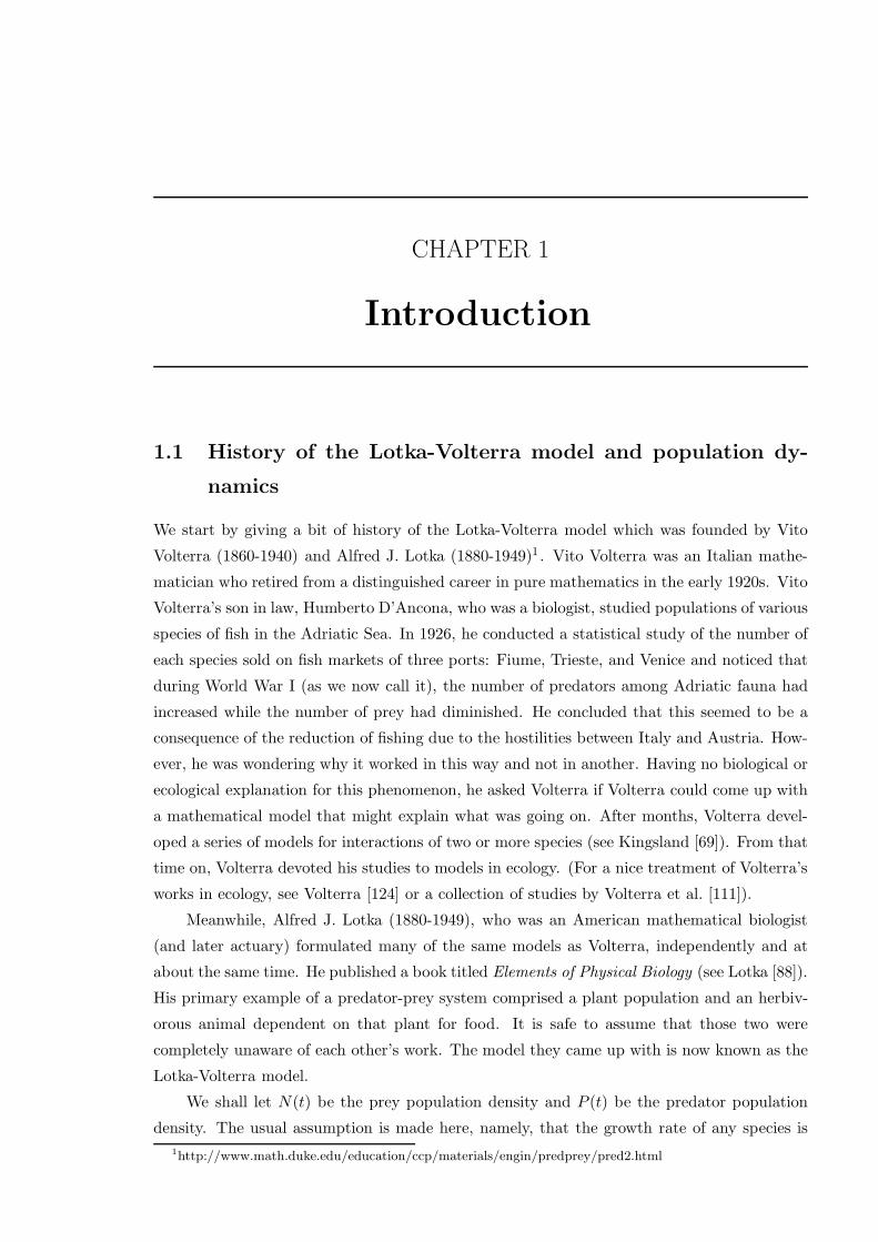
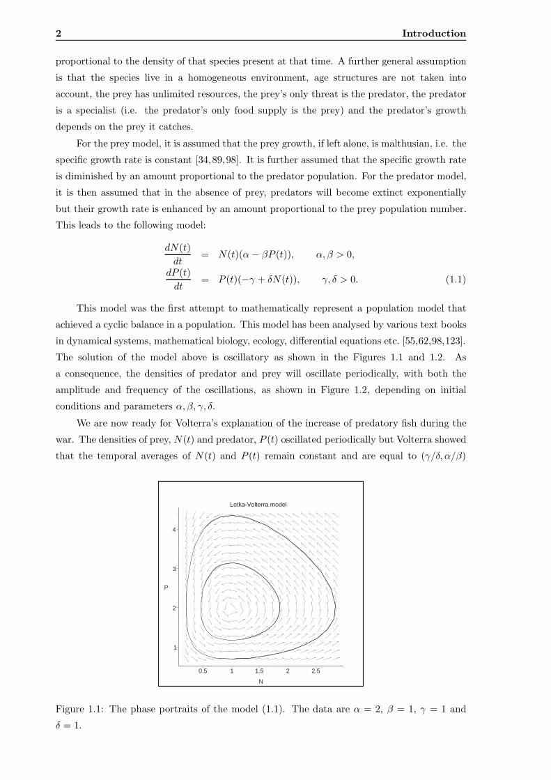
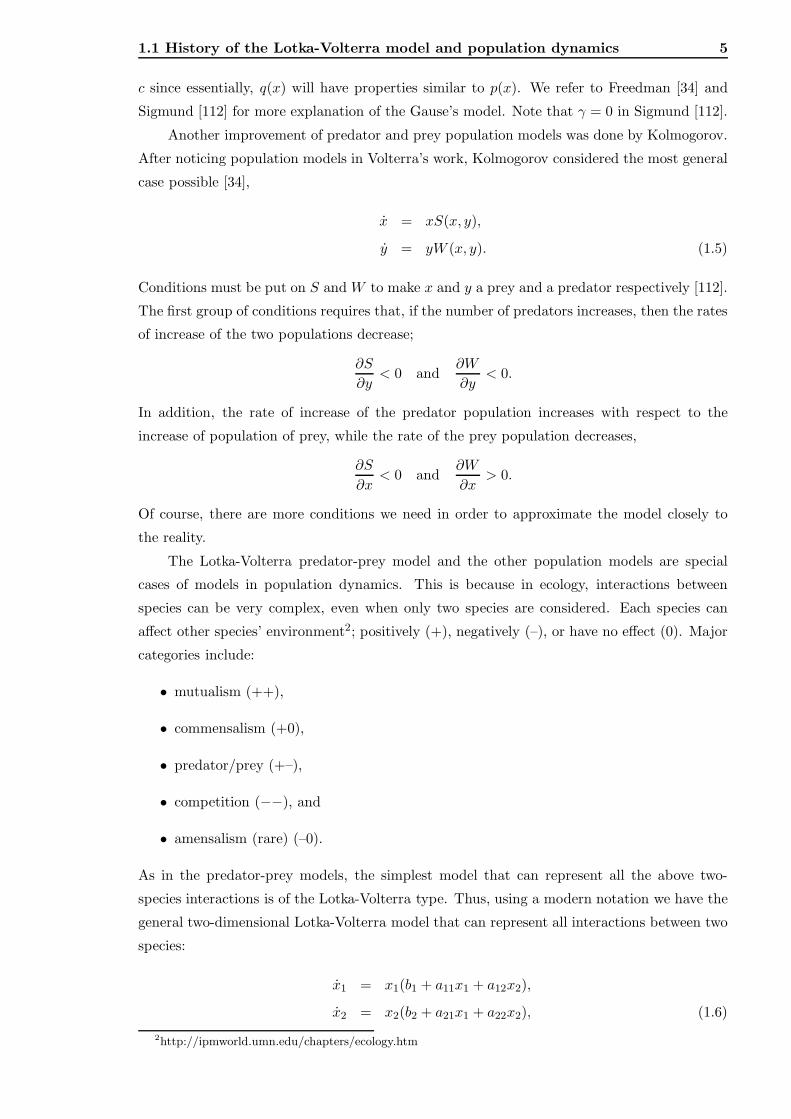
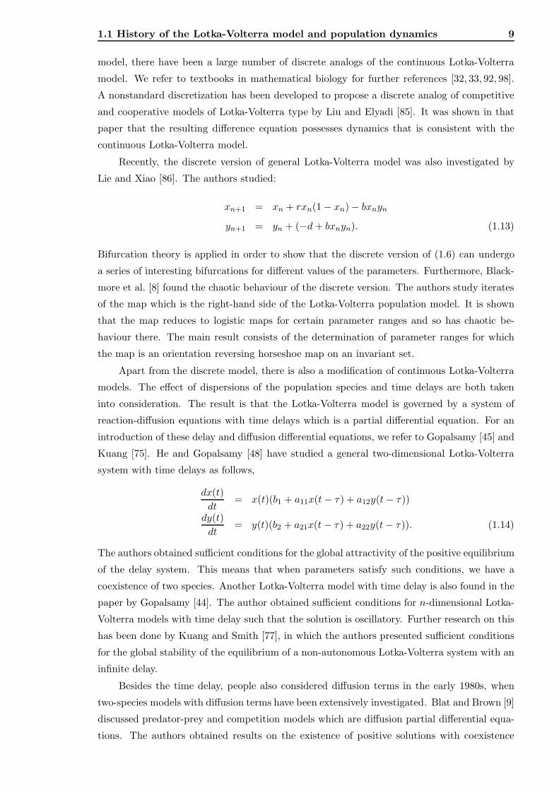
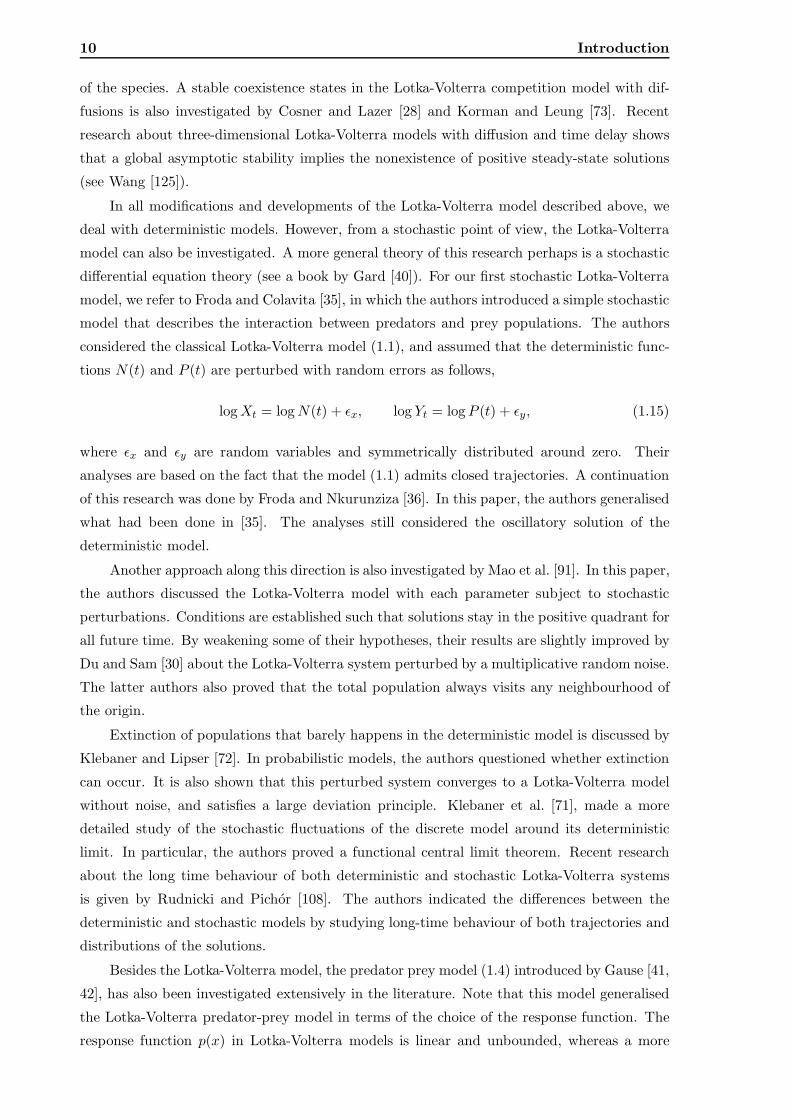
The solution of the model above is oscillatory as shown in the Figures 1.1 and 1.2. As
a consequence, the densities of predator and prey will oscillate periodically, with both the
amplitude and frequency of the oscillations, as shown in Figure 1.2, depending on initial
conditions and parameters α, β, γ, δ.
We are now ready for Volterra’s explanation of the increase of predatory fish during the
war. The densities of prey, N(t) and predator, P (t) oscillated periodically but Volterra showed
that the temporal averages of N(t) and P (t) remain constant and are equal to (γ/δ, α/β)
Lotka-Volterra model
1
2
3
4
P
0.5 1 1.5 2 2.5
N
Figure 1.1: The phase portraits of the model (1.1). The data are α = 2, β = 1, γ = 1 and
δ = 1.
1.1 History of the Lotka-Volterra model and population dynamics 3
1
2
3
4
N
0 5 10 15 20 25 30
t
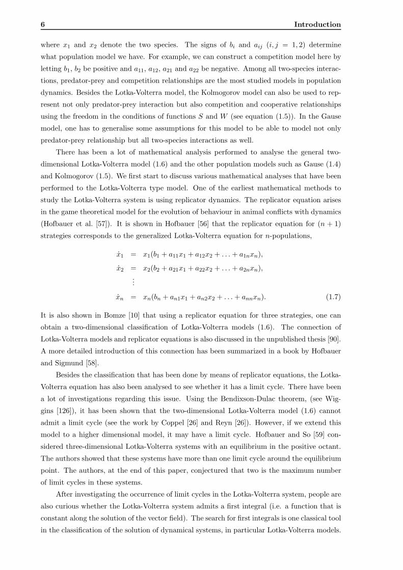
N,P
Figure 1.2: Periodic activity of prey (solid line) and predator (dotted line) populations, gen-
erated by the Lotka-Volterra model (1.1). The data are the same as those of Figure 1.1.
respectively. The supplementary contribution of fishing diminishes the quantity of α (the rate
of increase of the prey in the absence of predators) and increases the quantity of γ (the rate
of decrease of predators in the absence of prey). However, fishing does not affect the values of
β and δ, which measure the effects of the interaction between predators and their prey. Thus,
the time average of the population number of prey is now larger than in the unperturbed case.
In contrast, the time average of the population number of predators is now smaller than in
the unperturbed case, leading to an increase of predators and a decrease of prey that are just
what D’Ancona observed.
The model (1.1) has also been derived independently in the following fields:
1. epidemics (see Kermack and McKendrick [67,68]), with α = 0 and
• N are susceptible individuals and
• P are infective individuals,
2. ecology (Lotka [88] and Volterra [124]), with
• N are prey and
• P are predators,
3. combustion theory (see Hoppensteadt [61]), with
• N and P are chemical radicals formed during H2 and O2 combustion,
4. economics (see Hoppensteadt [61]), with
• N are the populace and
• P are predatory institution,
4 Introduction
and numerous studies from diverse disciplines.
The Lotka-Volterra model (1.1), from many points of view is unstable and unrealistic.
Firstly, in the absence of predators, the population of prey would grow exponentially towards
infinity. This feature is easily corrected, one way is to introduce a competition rate within the
prey species. We also assume that the density of prey, in the absence of predators, follows the
logistic model,dN(t)
dt= rN(t)(1 − N(t)
K), (1.2)
where r and K are positive constants. The constant r is the growth rate of the prey while
the constant K is the carrying capacity of the environment that limits the number of prey
population that can be considered as the competition rate as well. This logistic model was
first proposed by Verhulst in 1838 (see Murray [98]) to adjust the exponential growth of the
population model at that time. We then can add another term into the model (1.1) as an
intraspecific competition and if we wish, we may also allow an intraspecific competition within
the predators. The latter is less crucial, as their population does not explode anyway. This
leads to a more general Lotka-Volterra model as follows,
dN(t)
dt= N(t)(α − ηN(t) − βP (t)), α, β, η > 0,
dP (t)
dt= P (t)(−γ + δN(t) − κP (t)), γ, δ, κ > 0. (1.3)
Thus the classical model (1.1) is one special case of the above model.
Another reason why the classical model is unrealistic is the fact that the solution oscillates
periodically in the same periodic solution all the time. If a prey population increases, it
encourages growth of its predator. More predators however consume more prey, the population
of which starts to decline. With less food around, the predator population declines and when
it is low enough, this allows prey population to increase and the whole cycle starts over again.
Depending on the detailed system, such oscillations can grow or decay or go into a stable limit
cycle oscillation, which does not occur in either (1.1) or (1.3).
Georgii Frantsevitch Gause proposed another system of much more general equations
[41,42], which using modern notations x and y, take the following form:
x = xg(x) − yp(x),
y = y(−γ + q(x)), (1.4)
where x, y represent first derivatives of x and y with respect to time. Here g(x) is the specific
growth rate of the prey in the absence of any predators and p(x), q(x) are the response functions
for the predator with respect to that particular prey. The former function is positive on an
interval [0,K] and negative for x > K (because, for example, the food resources are limited, or
there is an intraspecific competition within the prey). We suppose that p is a positive function
with p(0) = 0, while q is strictly increasing for x > 0, has a negative limit when x decreases to
0 and a positive limit when x increases to +∞. These models are more reasonable and more
flexible than (1.1) and (1.3). In Gause’s model, he assumed that q(x) = cp(x) for some constant
1.1 History of the Lotka-Volterra model and population dynamics 5
c since essentially, q(x) will have properties similar to p(x). We refer to Freedman [34] and
Sigmund [112] for more explanation of the Gause’s model. Note that γ = 0 in Sigmund [112].
Another improvement of predator and prey population models was done by Kolmogorov.
After noticing population models in Volterra’s work, Kolmogorov considered the most general
case possible [34],
x = xS(x, y),
y = yW (x, y). (1.5)
Conditions must be put on S and W to make x and y a prey and a predator respectively [112].
The first group of conditions requires that, if the number of predators increases, then the rates
of increase of the two populations decrease;
∂S
∂y< 0 and
∂W
∂y< 0.
In addition, the rate of increase of the predator population increases with respect to the
increase of population of prey, while the rate of the prey population decreases,
∂S
∂x< 0 and
∂W
∂x> 0.
Of course, there are more conditions we need in order to approximate the model closely to
the reality.
The Lotka-Volterra predator-prey model and the other population models are special
cases of models in population dynamics. This is because in ecology, interactions between
species can be very complex, even when only two species are considered. Each species can
affect other species’ environment2; positively (+), negatively (–), or have no effect (0). Major
categories include:
• mutualism (++),
• commensalism (+0),
• predator/prey (+–),
• competition (−−), and
• amensalism (rare) (–0).
As in the predator-prey models, the simplest model that can represent all the above two-
species interactions is of the Lotka-Volterra type. Thus, using a modern notation we have the
general two-dimensional Lotka-Volterra model that can represent all interactions between two
species:
x1 = x1(b1 + a11x1 + a12x2),
x2 = x2(b2 + a21x1 + a22x2), (1.6)
2http://ipmworld.umn.edu/chapters/ecology.htm
6 Introduction
where x1 and x2 denote the two species. The signs of bi and aij (i, j = 1, 2) determine
what population model we have. For example, we can construct a competition model here by
letting b1, b2 be positive and a11, a12, a21 and a22 be negative. Among all two-species interac-
tions, predator-prey and competition relationships are the most studied models in population
dynamics. Besides the Lotka-Volterra model, the Kolmogorov model can also be used to rep-
resent not only predator-prey interaction but also competition and cooperative relationships
using the freedom in the conditions of functions S and W (see equation (1.5)). In the Gause
model, one has to generalise some assumptions for this model to be able to model not only
predator-prey relationship but all two-species interactions as well.
There has been a lot of mathematical analysis performed to analyse the general two-
dimensional Lotka-Volterra model (1.6) and the other population models such as Gause (1.4)
and Kolmogorov (1.5). We first start to discuss various mathematical analyses that have been
performed to the Lotka-Volterra type model. One of the earliest mathematical methods to
study the Lotka-Volterra system is using replicator dynamics. The replicator equation arises
in the game theoretical model for the evolution of behaviour in animal conflicts with dynamics
(Hofbauer et al. [57]). It is shown in Hofbauer [56] that the replicator equation for (n + 1)
strategies corresponds to the generalized Lotka-Volterra equation for n-populations,
x1 = x1(b1 + a11x1 + a12x2 + . . .+ a1nxn),
x2 = x2(b2 + a21x1 + a22x2 + . . .+ a2nxn),
...
xn = xn(bn + an1x1 + an2x2 + . . .+ annxn). (1.7)
It is also shown in Bomze [10] that using a replicator equation for three strategies, one can
obtain a two-dimensional classification of Lotka-Volterra models (1.6). The connection of
Lotka-Volterra models and replicator equations is also discussed in the unpublished thesis [90].
A more detailed introduction of this connection has been summarized in a book by Hofbauer
and Sigmund [58].
Besides the classification that has been done by means of replicator equations, the Lotka-
Volterra equation has also been analysed to see whether it has a limit cycle. There have been
a lot of investigations regarding this issue. Using the Bendixson-Dulac theorem, (see Wig-
gins [126]), it has been shown that the two-dimensional Lotka-Volterra model (1.6) cannot
admit a limit cycle (see the work by Coppel [26] and Reyn [26]). However, if we extend this
model to a higher dimensional model, it may have a limit cycle. Hofbauer and So [59] con-
sidered three-dimensional Lotka-Volterra systems with an equilibrium in the positive octant.
The authors showed that these systems have more than one limit cycle around the equilibrium
point. The authors, at the end of this paper, conjectured that two is the maximum number
of limit cycles in these systems.
After investigating the occurrence of limit cycles in the Lotka-Volterra system, people are
also curious whether the Lotka-Volterra system admits a first integral (i.e. a function that is
constant along the solution of the vector field). The search for first integrals is one classical tool
in the classification of the solution of dynamical systems, in particular Lotka-Volterra models.
1.1 History of the Lotka-Volterra model and population dynamics 7
One of the earliest attempt to find first integrals was the Carleman embedding method that
was used by Cairo et al. [15, 18]. Instead of finding the first integral, the authors obtained a
more general function that is called an invariant. This function depends on time not like a
first integral, which does not depend on time.
The Darboux method has also been used to find a first integral of the two-dimensional
Lotka-Volterra system (1.6) [20]. This method links the theory of algebraic solutions of differ-
ential equations to the search of the first integral or the integrating factor. Extensive results
have been found by Cairo and Llibre [22] in which algebraic solutions of degree one to four
have been found. Consequently, the first integral or the integrating factor can be found. The
integrating factor, in the end, can be used to find the first integral even when it is not trivial.
Polynomial inverse integrating factors have been introduced by Cairo et al. [24] to show the
integrability of Lotka-Volterra models via polynomial first integrals. Finally a more recent
result in the integrability of Lotka-Volterra systems is found by Cairo et al. [21] where the
complete classification of Liouvillian first integrals for the quadratic Lotka-Volterra model
was presented. More detail about the Liouvillian first integral can be found in a paper by
Singer [113]. Another recent result is found in Llibre and Valls (2007) [87], where the authors
provided a complete classification of all Lotka-Volterra systems having a global first integral.
All results listed above are discussing the two-dimensional Lotka-Volterra model except
the ones that were using the Carleman embedding method, in which the authors studied
n-dimensional models. In the three-dimensional model, there have been a lot of discussions
as well, see Grammaticos [46], Labrunie [81] and Moulin Ollagnier [96]. The authors have
studied the integrability of three-dimensional Lotka-Volterra models that depend on three
parameters via polynomial first integrals. The model that is discussed is a special case of
general Lotka-Volterra system (1.7) for n = 3:
x = x(Cy + z),
y = y(Az + x),
z = z(Bx+ y). (1.8)
Darboux integrability has also been used to show the integrability of three-dimensional sys-
tems, Cairo and Llibre [14,23]. Also, Moulin Ollagnier [97] classified conditions for the three
parameters for which the three-dimensional Lotka-Volterra systems have a Liouvillian first
integral of degree zero.
Other methods such as Hamiltonian method [16,38,63,64], direct and indirect integrating
method [37, 39] have also been applied to find integrals of two and three-dimensional Lotka-
Volterra systems.
Other than first integrals, other geometrical structures in Lotka-Volterra models have
also been investigated. It has been shown in Schimming [110] that necessary and sufficient
conditions can be found on the Lotka-Volterra models to admit a conservation law. The defi-
nition of conservative can be found in that paper. Hamiltonian structure is also investigated
by Plank [102]. The author derived conditions for two-dimensional Lotka-Volterra equations
to have a Hamiltonian structure in the first part of his paper. The second part discussed
8 Introduction
that the Hamiltonian structure that the author derived in the two-dimensional case can also
be used as an Ansatz for possible Hamiltonian functions and invariants of the n-dimensional
case. Another result concerning the Hamiltonian structure is also discussed by the same au-
thor, Plank [103], in which the author discussed the dynamics of n-dimensional Lotka-Volterra
system having an invariant hyperplane.
Finally, in McLachlan and Quispel [93, sec 3.14] and references therein, various special
structures of Lotka-Volterra systems are discussed. Instead of writing the n-dimensional model
as in (1.7), the authors wrote the system (1.7) as follows:
xi = xi
bi +
n∑
j=1
aijxj
, i = 1, .., n. (1.9)
In the domain xi > 0, the authors defined ui := log xi, to get:
ui = bi +
n∑
j=1
aijeuj (1.10)
or
u = b +Aeu, (1.11)
where u = (u1, u2, . . . , un)T , b = (b1, b2, . . . , bn)T and A = [aij ]. Each Lotka-Volterra system
falls into one or both of the following cases:
1. b ∈ range(A),
2. rank(A) < n.
In case (1), the system (1.11) can be re-written in a linear gradient form [94]:
u = A∇V (u), (1.12)
with V (u) =∑
i(eui + ciui). Some special cases are:
1. if A is symmetric positive definite, (1.12) is a gradient system;
2. if A+AT is negative definite ( [111,124]), then (1.12) has V as a Lyapunov function;
3. if A is antisymmetric, (1.12) is either Hamiltonian system (if rank(A) = n) or a Poisson
system (if rank(A) < n)
4. if aii = 0 for all i, then (1.12) is divergence free [111,124].
In recent investigations, it is shown that many economic, physical, and biological phenom-
ena are best represented via difference equations instead of differential equations, Agarwal [2].
There are also situations for which differential equations are the best fit, however the solution of
the differential equations is hard to get. One may then use some numerical scheme to transform
the given differential equation into a difference equation, Mickens [95]. The resulting difference
equation should be dynamically consistent with its continuous version. Analysis of discrete
dynamical systems has been done (see, for instance Wiggins [126]). In the Lotka-Volterra
1.1 History of the Lotka-Volterra model and population dynamics 9
model, there have been a large number of discrete analogs of the continuous Lotka-Volterra
model. We refer to textbooks in mathematical biology for further references [32, 33, 92, 98].
A nonstandard discretization has been developed to propose a discrete analog of competitive
and cooperative models of Lotka-Volterra type by Liu and Elyadi [85]. It was shown in that
paper that the resulting difference equation possesses dynamics that is consistent with the
continuous Lotka-Volterra model.
Recently, the discrete version of general Lotka-Volterra model was also investigated by
Lie and Xiao [86]. The authors studied:
xn+1 = xn + rxn(1 − xn) − bxnyn
yn+1 = yn + (−d+ bxnyn). (1.13)
Bifurcation theory is applied in order to show that the discrete version of (1.6) can undergo
a series of interesting bifurcations for different values of the parameters. Furthermore, Black-
more et al. [8] found the chaotic behaviour of the discrete version. The authors study iterates
of the map which is the right-hand side of the Lotka-Volterra population model. It is shown
that the map reduces to logistic maps for certain parameter ranges and so has chaotic be-
haviour there. The main result consists of the determination of parameter ranges for which
the map is an orientation reversing horseshoe map on an invariant set.
Apart from the discrete model, there is also a modification of continuous Lotka-Volterra
models. The effect of dispersions of the population species and time delays are both taken
into consideration. The result is that the Lotka-Volterra model is governed by a system of
reaction-diffusion equations with time delays which is a partial differential equation. For an
introduction of these delay and diffusion differential equations, we refer to Gopalsamy [45] and
Kuang [75]. He and Gopalsamy [48] have studied a general two-dimensional Lotka-Volterra
system with time delays as follows,
dx(t)
dt= x(t)(b1 + a11x(t− τ) + a12y(t− τ))
dy(t)
dt= y(t)(b2 + a21x(t− τ) + a22y(t− τ)). (1.14)
The authors obtained sufficient conditions for the global attractivity of the positive equilibrium
of the delay system. This means that when parameters satisfy such conditions, we have a
coexistence of two species. Another Lotka-Volterra model with time delay is also found in the
paper by Gopalsamy [44]. The author obtained sufficient conditions for n-dimensional Lotka-
Volterra models with time delay such that the solution is oscillatory. Further research on this
has been done by Kuang and Smith [77], in which the authors presented sufficient conditions
for the global stability of the equilibrium of a non-autonomous Lotka-Volterra system with an
infinite delay.
Besides the time delay, people also considered diffusion terms in the early 1980s, when
two-species models with diffusion terms have been extensively investigated. Blat and Brown [9]
discussed predator-prey and competition models which are diffusion partial differential equa-
tions. The authors obtained results on the existence of positive solutions with coexistence
10 Introduction
of the species. A stable coexistence states in the Lotka-Volterra competition model with dif-
fusions is also investigated by Cosner and Lazer [28] and Korman and Leung [73]. Recent
research about three-dimensional Lotka-Volterra models with diffusion and time delay shows
that a global asymptotic stability implies the nonexistence of positive steady-state solutions
(see Wang [125]).
In all modifications and developments of the Lotka-Volterra model described above, we
deal with deterministic models. However, from a stochastic point of view, the Lotka-Volterra
model can also be investigated. A more general theory of this research perhaps is a stochastic
differential equation theory (see a book by Gard [40]). For our first stochastic Lotka-Volterra
model, we refer to Froda and Colavita [35], in which the authors introduced a simple stochastic
model that describes the interaction between predators and prey populations. The authors
considered the classical Lotka-Volterra model (1.1), and assumed that the deterministic func-
tions N(t) and P (t) are perturbed with random errors as follows,
logXt = logN(t) + ǫx, log Yt = logP (t) + ǫy, (1.15)
where ǫx and ǫy are random variables and symmetrically distributed around zero. Their
analyses are based on the fact that the model (1.1) admits closed trajectories. A continuation
of this research was done by Froda and Nkurunziza [36]. In this paper, the authors generalised
what had been done in [35]. The analyses still considered the oscillatory solution of the
deterministic model.
Another approach along this direction is also investigated by Mao et al. [91]. In this paper,
the authors discussed the Lotka-Volterra model with each parameter subject to stochastic
perturbations. Conditions are established such that solutions stay in the positive quadrant for
all future time. By weakening some of their hypotheses, their results are slightly improved by
Du and Sam [30] about the Lotka-Volterra system perturbed by a multiplicative random noise.
The latter authors also proved that the total population always visits any neighbourhood of
the origin.
Extinction of populations that barely happens in the deterministic model is discussed by
Klebaner and Lipser [72]. In probabilistic models, the authors questioned whether extinction
can occur. It is also shown that this perturbed system converges to a Lotka-Volterra model
without noise, and satisfies a large deviation principle. Klebaner et al. [71], made a more
detailed study of the stochastic fluctuations of the discrete model around its deterministic
limit. In particular, the authors proved a functional central limit theorem. Recent research
about the long time behaviour of both deterministic and stochastic Lotka-Volterra systems
is given by Rudnicki and Pichor [108]. The authors indicated the differences between the
deterministic and stochastic models by studying long-time behaviour of both trajectories and
distributions of the solutions.
Besides the Lotka-Volterra model, the predator prey model (1.4) introduced by Gause [41,
42], has also been investigated extensively in the literature. Note that this model generalised
the Lotka-Volterra predator-prey model in terms of the choice of the response function. The
response function p(x) in Lotka-Volterra models is linear and unbounded, whereas a more
1.1 History of the Lotka-Volterra model and population dynamics 11
reasonable response function should be non-linear and bounded. For more conditions that
response functions should behave, we refer to a book by Freedman [34]. Holling [60] introduced
a more reasonable response function to model the predator-prey relationship. Since then,
various response functions have been introduced and analysed to model various interactions
of predator-prey models. For instance, we refer to a paper by Kuang [74], in which the author
has studied a response function with strictly concave down isocline and shown the existence
of at least three limit cycles in the corresponding model.
Ruan and Xiao [107] studied a global analysis of a predator-prey model of Gause type
using a bifurcation theory. The authors used the following response function,
p(x) =mx
a+ bx+ cx2, (1.16)
that is usually called a Holling type-IV function. The authors have studied the case where
b = 0 and shown that their model exhibited a number of bifurcations. Moreover, it has been
shown that a limit cycle cannot coexist with a homoclinic bifurcation for all parameters as a
part of a codimension-two bifurcation. This research is extended by Zhu et al. [131] with a
positive b. Rothe and Shafer [106] have actually studied the same model with a negative b.
Both these papers have performed bifurcation analysis to classify the predator-prey model with
Holling type-IV response functions. The authors have shown that if the population of prey is
large enough, then the extinction of predators occurs regardless of the initial size of predator
population. The authors have also shown that the coexistence of predator and prey can be
in the form of a steady-state solution or a periodic solution. More focused research about
limit cycles or periodic solutions of the predator-prey model with Holling type-IV response
functions has been performed by Xiao and Zhu [129].
However, recent investigations and empirical evidence showed that the most natural sys-
tem (i.e. approximating the reality) should not be using a response function that is prey-
dependent (i.e. p(x)). Instead, the response function should depend on a ratio of prey and
predator populations (i.e. p(x/y)). For more biological explanations, we refer to Akcakaya
et al. [3] and extensive references cited therein. Research on the ratio-dependent model has
revealed rich interesting dynamics such as deterministic extinctions, existences of multiple
attractors, and existences of stable limit cycles. Moreover, it was shown in the paper by
Jost et al. [65] that the ratio-dependent model has such a complex dynamics near the origin
(0, 0). The authors have studied the analytical behaviour at (0, 0) and demonstrated that this
equilibrium can be either a saddle point or an attractor which has an important implication
concerning the global behaviour of the model. If the origin is an atractor then we have the
case of deterministic extinction.
Kuang and Beretta [76] have studied a ratio-dependent predator-prey model that used
the following response function,
p(x) =mx
a+ x. (1.17)
This function is usually called a Holling type-II function (see all the references therein). The
authors modified the function into p(x/y) and performed a global qualitative analysis and
showed that the positive steady-state solution is asymptotically stable for some parameters.
12 Introduction
The authors also gave conditions for the other three equilibria to be globally asymptotically
stable. A continuation along this line of research has been performed in the paper by Tang
and Zhang [117], in which the authors obtained some conditions on parameters such that the
system has a heteroclinic loop.
To conclude the discussion of Gause-type predator-prey population models, we refer to
a paper by Cosner et al. [27] for the derivation of various forms of functional responses in
predator-prey models. In some conditions where the predators are assumed to have a homo-
geneous spatial distribution, the suitable functional response is prey-dependent, however if the
predators are assumed to form a dense colony in a single (possibly moving) location, or if the
region where predators can encounter prey is assumed to be of limited size then the functional
response depends on the ratio of prey and predators (i.e. the ratio dependence model).
One more reason why Lotka-Volterra equations have attracted ample attention is because
chaotic behaviour may occur in higher-dimensional models. One of the first investigations,
showing that the Lotka-Volterra model can exhibit such a behaviour is Smale [114]. The author
studied a general competition model and argued that under some conditions, any asymptotic
dynamical behaviour is possible for populations of five or more species. The occurrence of
chaos through quasi-periodic orbits perhaps was first found by Arneodo et al. [4]. The authors
of this paper studied one-parameter families of one class of three-dimensional Lotka-Volterra
systems. Hirsch in his series of papers [49–54] has studied a differential equation that is
competitive or cooperative and shown that in the Lotka-Volterra competition (or cooperative)
equation with n ≤ 3 (i.e. three or less species interaction), no chaotic behaviours are possible,
and thus, the model with n = 4 is the simplest example where chaotic solutions are possible,
as it was shown by Vano et al. [122].
From the point of view of applications, Lokta-Volterra systems have also intrigued a large
number of people. The first application that can be represented by this model is of course
a population dynamics model. Moreover, the Lotka-Volterra equation can be used to model
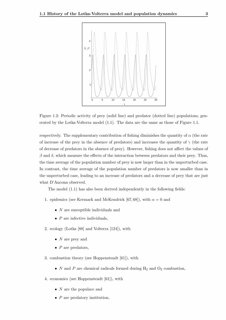
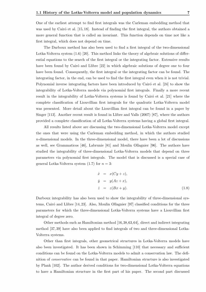
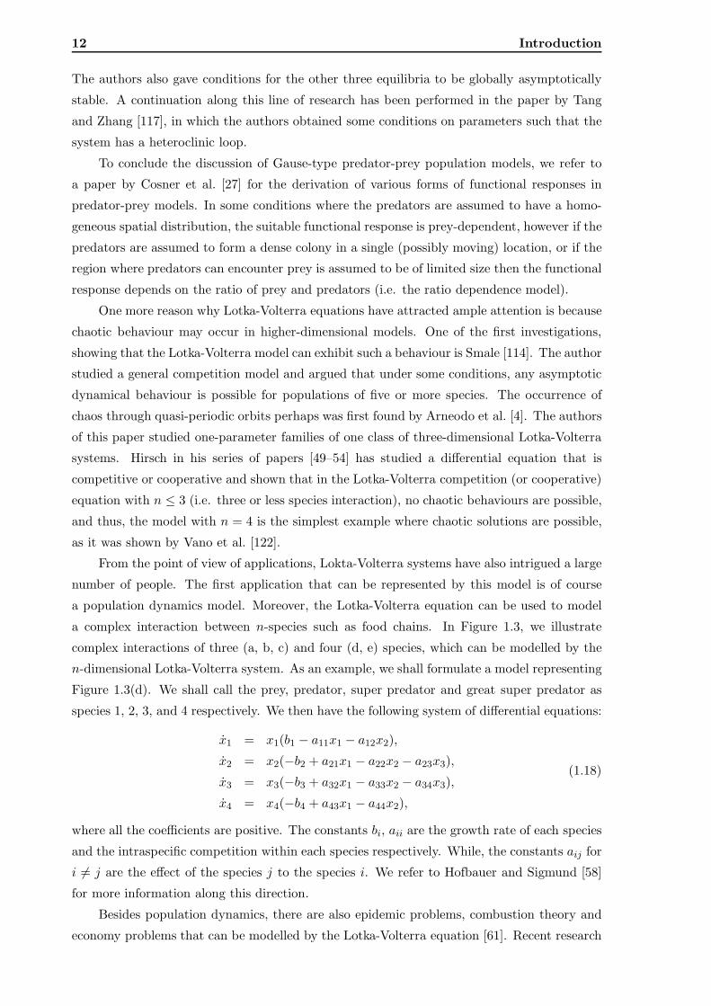
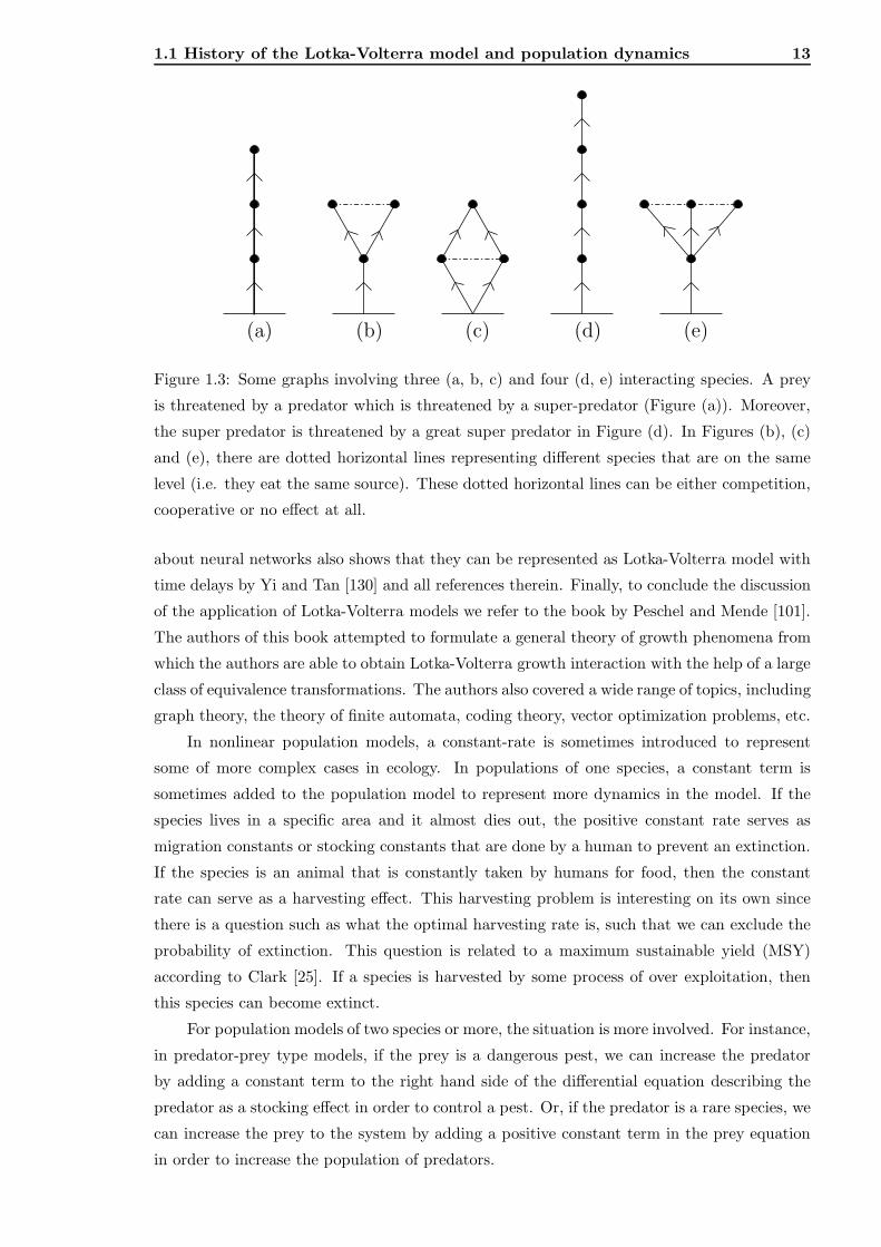
a complex interaction between n-species such as food chains. In Figure 1.3, we illustrate
complex interactions of three (a, b, c) and four (d, e) species, which can be modelled by the
n-dimensional Lotka-Volterra system. As an example, we shall formulate a model representing
Figure 1.3(d). We shall call the prey, predator, super predator and great super predator as
species 1, 2, 3, and 4 respectively. We then have the following system of differential equations:
x1 = x1(b1 − a11x1 − a12x2),
x2 = x2(−b2 + a21x1 − a22x2 − a23x3),
x3 = x3(−b3 + a32x1 − a33x2 − a34x3),
x4 = x4(−b4 + a43x1 − a44x2),
(1.18)
where all the coefficients are positive. The constants bi, aii are the growth rate of each species
and the intraspecific competition within each species respectively. While, the constants aij for
i 6= j are the effect of the species j to the species i. We refer to Hofbauer and Sigmund [58]
for more information along this direction.
Besides population dynamics, there are also epidemic problems, combustion theory and
economy problems that can be modelled by the Lotka-Volterra equation [61]. Recent research
1.1 History of the Lotka-Volterra model and population dynamics 13
(a) (b) (c) (d) (e)
Figure 1.3: Some graphs involving three (a, b, c) and four (d, e) interacting species. A prey
is threatened by a predator which is threatened by a super-predator (Figure (a)). Moreover,
the super predator is threatened by a great super predator in Figure (d). In Figures (b), (c)
and (e), there are dotted horizontal lines representing different species that are on the same
level (i.e. they eat the same source). These dotted horizontal lines can be either competition,
cooperative or no effect at all.
about neural networks also shows that they can be represented as Lotka-Volterra model with
time delays by Yi and Tan [130] and all references therein. Finally, to conclude the discussion
of the application of Lotka-Volterra models we refer to the book by Peschel and Mende [101].
The authors of this book attempted to formulate a general theory of growth phenomena from
which the authors are able to obtain Lotka-Volterra growth interaction with the help of a large
class of equivalence transformations. The authors also covered a wide range of topics, including
graph theory, the theory of finite automata, coding theory, vector optimization problems, etc.
In nonlinear population models, a constant-rate is sometimes introduced to represent
some of more complex cases in ecology. In populations of one species, a constant term is
sometimes added to the population model to represent more dynamics in the model. If the
species lives in a specific area and it almost dies out, the positive constant rate serves as
migration constants or stocking constants that are done by a human to prevent an extinction.
If the species is an animal that is constantly taken by humans for food, then the constant
rate can serve as a harvesting effect. This harvesting problem is interesting on its own since
there is a question such as what the optimal harvesting rate is, such that we can exclude the
probability of extinction. This question is related to a maximum sustainable yield (MSY)
according to Clark [25]. If a species is harvested by some process of over exploitation, then
this species can become extinct.
For population models of two species or more, the situation is more involved. For instance,
in predator-prey type models, if the prey is a dangerous pest, we can increase the predator
by adding a constant term to the right hand side of the differential equation describing the
predator as a stocking effect in order to control a pest. Or, if the predator is a rare species, we
can increase the prey to the system by adding a positive constant term in the prey equation
in order to increase the population of predators.
14 Introduction
This research perhaps is first done by Brauer and Sanchez [11]. The authors discussed
how the stability of an equilibrium is affected by the introduction of the constant term. Various
population models that were discussed include: logistic models, modified logistic models and
logistic models with time delays and two-dimensional Lotka-Volterra competition models.
More advanced techniques are performed in the paper by Xiao and Ruan [128] and Xiao
and Jennings [127], in which the authors performed a bifurcation analysis on a Gause-type
predator-prey model and found numerous interesting bifurcations. This bifurcation then can
be used to find the optimal harvesting as the constant term is one of the parameters that are
varied.
Although there has been much progress since the introduction of Lotka-Volterra equations
and other population models almost a century ago, certain questions remain unanswered, in
particular: to the author’s best knowledge, the consequences of constant terms in Lotka-
Volterra equations. This thesis will address, amongst other things, the global analysis of
general two-dimensional Lotka-Volterra systems with constant terms which we will analyse
using a dynamical systems theory.
1.2 Motivation of this thesis
The main topic of this thesis is about the general Lotka-Volterra system with constant terms.
As is mentioned in the title of this thesis, we will perform a semi-global analysis of this
system. Thus, this thesis is a collection of studies on Lotka-Volterra systems with constant
terms. Dynamical systems theory will underline our analysis. We use the word “semi” mainly
because dynamical systems theories are very broad and we only use some of those theories to
analyse the Lotka-Volterra system with constant terms. Special attention will be given to the
following areas in dynamical systems theory in this thesis:
1. bifurcation theory of differential equations,
2. integrability of differential equations.
As is mentioned in the previous section, the Lotka-Volterra system has arisen frequently in
mathematical publications. The first issue that we want to discuss concerns two-dimensional
Lotka-Volterra systems with a constant term. The discussion involves the theory of bifurcation
analysis. Although some aspect of the two-dimensional Lotka-Volterra system with constant
terms have been discussed, such as the stability of the positive equilibrium, the stability of
the origin (as it represents extinction in the real world), Brauer and Sanchez [11], we believe
that a global analysis of general two-dimensional Lotka-Volterra systems with constant terms
has not been studied.
Bifurcations of general Lotka-Volterra equations have received less attention in the lit-
erature. One of the reasons for this is the structure that is possessed by such systems. In
bifurcation theory, the presence of special structure complicates the analysis, since it usually
leads to certain degeneracies that one does not normally have. This leads us to then analyse
a general dynamical system with the same special structure as the Lotka-Volterra system.
1.3 Mathematical preliminaries 15
The next issue that is dealt with in this thesis is the existence of first integrals of a
dynamical system. It is known that the classical Lotka-Volterra system (1.1) has a first
integral for every value of the parameters, in fact it was Volterra himself who proved that
it admits a function that is constant with respect to time, (see the book by Hofbauer and
Sigmund (1998) [58]). It is also known that the problem of searching for a first integral of
general Lotka-Volterra systems (1.7) is still a topic of ongoing research. If we add constant
terms to the system, a natural question would be whether the first integral is still preserved
and the conditions on the parameters can still be obtained in the presence of the constant
terms.
Our goal in this thesis is to provide some mathematical insight into a class of mathematical
models of Lotka-Volterra type that arise quite often in the literature. However, we also try to
make the connection to other fields as clear as possible. We hope that this work is as enjoyable
to read as it was to produce.
1.3 Mathematical preliminaries
In this section, we will describe some mathematical terminology that we are going to use
throughout the thesis. We will discuss some concepts that we use in this thesis to understand
the Lotka-Volterra system with constant terms and discuss why these aspects are important.
1.3.1 Continuous dynamical systems
In this thesis, we will study differential equations of the following form,
x = F (x, µ), (1.19)
where x ∈ U ⊂ Rn and µ ∈ V ⊂ R
p, with U and V being open sets in Rn and R
p respectively.
The function on the right hand side will always be assumed to be in Cr (i.e. the derivatives
F ′, F ′′, . . . , F (r) exist and are continuous) with r being defined as we go along. The overdot
means “ ddt
”. We refer the differential equation (1.19) as a continuous dynamical system or a
vector field. By a solution of (1.19) we mean a continuously differentiable function, x from
some interval I ⊂ R1 into R
n, which we represent as follows
x : I → Rn,
t 7→ x(t),(1.20)
such that x(t) satisfies (1.19), i.e. x(t) = F (x(t), t, µ). A solution x(t) usually depends on
an initial condition x0 ∈ U , therefore it is common to write the solution of the differential
equation as x(t, x0). We view the variables µ as parameters that are kept constant when we
consider the solution of this differential equation. The phase space is referred as the space
of the dependent variable x. Abstractly, our goal is to understand the geometry of solutions
curves in this phase space.
One trivial solution in the continuous dynamical system is called an equilibrium which is
a point in phase space, x0 which is kept invariant under the flow of the dynamical system i.e.
16 Introduction
F (x0) = 0. Other terms, often used for the term “equilibrium”, are “fixed point”, “critical
point” or “steady state”. Another interesting solution is a periodic solution. i.e. a non
steady-state solution of (1.19) that satisfies x(t+ T ) = x(t), for a T 6= 0.
Let x0 be an equilibrium. A solution x(t) satisfying
limt→±∞
x(t) = x0, (1.21)
is called a homoclinic solution (homoclinic loop). Another interesting object that we will
also see in this thesis is a heteroclinic solution (heteroclinic connection). Let x0 and x1 be
two distinct equilibria and a heteroclinic solution is defined as a non-constant solution, x(t),
satisfying
limt→∞
x(t) = x0, and limt→−∞
x(t) = x1. (1.22)
Remark that homoclinic and heteroclinic solutions only occurs on specific values of parameters.
We also want to look for an invariant manifold, i.e. a manifold, M ⊂ Rn such that x(t) ∈ M
for all t. The invariant manifold might have a special geometry such as an invariant sphere or
an invariant torus.
1.3.2 First integrals
For a general autonomous dynamical system,
x = f(x), x ∈ Rn, (1.23)
where f(x) = F (x, µ0), (we fixed µ = µ0), a scalar valued function H(x) is said to be a first
integral if it is constant along the solution x(t) of the differential equation above, i.e.,
dH(x(t))
dt= ∇H(x) · x = ∇H(x) · f(x) = 0,
where “·” denotes the usual Euclidean inner product. From this relation, we see that the level
sets of H(x) (which are generally (n−1)-dimensional) are invariant sets. For two-dimensional
dynamical systems, the level sets actually give the trajectory of the solution of the system.
For this reason, in this thesis we discuss the first integral of the Lotka-Volterra system with
constant terms which is in fact two-dimensional. By searching a first integral of this system
for some values of the parameters, we can compute the solution of the system.
1.3.3 Stability of an equilibrium
In this section, we would like to briefly discuss the idea of stability. The stability of each in-
variant structure we have described above (i.e. equilibrium, periodic, homoclinic, heteroclinic
solutions etc.) is important because it determines the dynamics of solutions of the vector field.
Here we use mainly two different stability types: neutrally stable (or Lyapunov-stable) and
asymptotically stable. In a neutrally stable situation, nearby solutions stay close to the invari-
ant structure as time increases while in an asymptotically stable situation, nearby solutions
get attracted. In addition, we also have the notion of local stability and global stability. In
1.3 Mathematical preliminaries 17
this discussion, we restrict ourselves to discuss the local stability of an equilibrium as it will
lead to the stability of other invariant structures.
Our first step is to understand the nature of solutions near an equilibrium x0 with initial
conditions close to x0 (local stability), we will linearize our vector field (1.23). Let,
x = x0 + y. (1.24)
Substituting (1.24) into (1.23) and Taylor expanding about x0 gives,
x = x0 + y = f(x0) +Df(x0)y + O(‖y‖2), (1.25)
where Df denotes the first derivative of f and ‖ · ‖ is a norm in Rn (note: in order to obtain
(1.25), f must be at least twice differentiable). Using the fact that x0 = f(x0) = 0, we have
y = Df(x0)y + O(‖y‖2). (1.26)
The equation above describes the evolution of solutions near x0, so it seems reasonable to
understand the behaviour of the solution close to x0 by studying the associated linear system,
y = Df(x0)y. (1.27)
Therefore, the question of stability of x0 involves the following steps:
1. determine the stability of y = 0,
2. show that the stability of y = 0 implies the stability of x0, and
3. determine the stability of y = 0 as parameters are varied.
The first step is really an elementary linear differential equation problem, thus if all eigenvalues
of Df(x0) have non-zero real parts, then the fixed point y = 0 is hyperbolic, moreover if
all eigenvalues of Df(x0) have negative (positive) real parts then the fixed point y = 0 is
asymptotically stable (unstable resp.) To answer the second part, we refer to a theorem by
Hartman-Grobman (see Guckenheimer and Holmes [47]),
Theorem 1.1 (Hartman-Grobman). If Df(x0) has no zero or purely imaginary eigenvalues
then there is a homeomorphism h defined on some neighbourhood U of x0 in Rn locally taking
orbits of the vector field (1.23) to those of the linear vector field (1.27). The homeomorphism
preserves the sense of orbits and can also be chosen to preserve parametrization by time.
This theorem really means that the stability of the hyperbolic equilibrium solution, x0
and the nature of solutions near this point are determined by the linearization. However,
if the matrix Df(x0) has an eigenvalue that has a zero real part (non-hyperbolic), then the
stability cannot be determined by the linearization. We will discuss the issue regarding the
stability of vector fields having a zero real part eigenvalue later on.
The third step is really the main question in bifurcation theory, as when we vary pa-
rameters in our dynamical system, the equilibrium might undergo a change of stability and
moreover, the qualitative structure of solutions of the vector field might change as well. This
18 Introduction
phenomenon is known as bifurcation. To understand when and how the qualitative structure
of solutions of the vector field is changed we define the notion of conjugacy and equivalence of
vector fields. Two vector fields on Rn are said to be topologically equivalent if there exists a
homeomorphism h : Rn → R
n that maps orbits of the first vector field to orbits of the second
vector field in such a way that the homeomorphism preserves orientation but not necessarily
parametrization by time. If h does preserve parametrization by time, then the dynamics gen-
erated by those vector field are said to be conjugate. Let us consider a vector field depending
on one parameter, i.e., x = fµ(x), where x ∈ Rn and µ ∈ R. It is said that the vector field
undergoes a bifurcation at µ = µ0 if vector fields x = fµ<µ0(x) are not conjugate with vector
fields x = fµ>µ0(x). It is also said that the vector field x = fµ0
(x) is structurally stable if
there is ǫ > 0 such that vector fields x = fµ(x) are conjugate with x = fµ0(x) if |µ− µ0| < ǫ.
Here we define the notions of conjugacy and structural stability in terms of one parameter
but we can extend these definitions to the vector field having more than one parameter. We
remark that conjugacies do not need to be defined on all Rn but, rather, on appropriately
chosen open sets in Rn especially an open set near the fixed point. It has been proven that
the dynamics near a hyperbolic fixed point is structurally stable [47, chapter 1].
1.3.4 Center manifold theorem
In this section, we discuss one of the techniques necessary for the analysis of bifurcation
problems. We will discuss the vector field having a non-hyperbolic fixed point, i.e., the matrix
Df(x0) has a zero real-part eigenvalue. We first introduce the following theorem,
Theorem 1.2. Let x = f(x) be a vector field on Rn, x0 is an equilibrium and let A = Df(x0).
Divide the spectrum of A into three parts, σs, σu and σc with,
Re λ
< 0, if λ ∈ σs;
= 0, if λ ∈ σc;
> 0, if λ ∈ σu.
(1.28)
Let the eigenspaces of σs, σu and σc be Es, Eu and Ec respectively. Then there exist stable and
unstable invariant manifolds W s and W u tangent to Es and Eu at x0 and a center manifold
W c tangent to Ec at x0. The stable and unstable manifolds are unique but W c does not need
to be.
For more information on the existence, uniqueness and smoothness of these invariant
manifolds and for a proof of this theorem, we refer to books on dynamical systems theory
[47,126] and references therein.
Without loss of generality, we assume that x0 is the origin, i.e. (0, 0, 0) ∈ Rc × R
s × Ru.
This theorem implies that the system having a non-hyperbolic fixed point, x0, is locally
topologically equivalent with,
xc = Acxc + fc(xc, xs, xu),
xs = Asxs + fs(xc, xs, xu),
xu = Auxu + fu(xc, xs, xu) (xc, xs, xu) ∈ Rc × R
s × Ru, (1.29)
1.3 Mathematical preliminaries 19
wherefc(0, 0, 0) = 0, Dfc(0, 0, 0) = 0,
fs(0, 0, 0) = 0, Dfs(0, 0, 0) = 0,
fu(0, 0, 0) = 0, Dfu(0, 0, 0) = 0.
(1.30)
In the above, Ac is a c× c matrix having eigenvalues with zero real parts, As and Au are s× sand u× u matrices having eigenvalues with negative and positive real parts respectively. The
case of interest is when the space σu is empty, hence we are left with these following equations,
xc = Acxc + fc(xc, xs),
xs = Asxs + fs(xc, xs), (xc, xs) ∈ Rc × R
s. (1.31)
Since the center manifold is tangent to Ec (the space xs = 0), then we can represent it as a
(local) graph
W c = {(xc, xs)|xs = h(xc)}, h(0) = Dh(0) = 0, (1.32)
where h is defined in some small neighbourhood U ⊂ Rc of the origin. The dynamics of the
vector field restricted to the center manifold is,
xc = Acxc + fc(xc, h(xc)). (1.33)
The following theorem by Henry and Carr [47] that describes the dynamics of the vector field
restricted to the center manifold (1.33) locally near the origin provides a good approximation
to the flow (1.31) near the origin.
Theorem 1.3. If the origin of (1.33) is locally asymptotically stable (unstable) then the origin
of (1.31) is also asymptotically stable (unstable resp.).
However, if we include the unstable direction (the space σu), the theorem above does not
apply. It is still useful, though, to consider the dynamics restricted to the center manifold as
it can be used to start our bifurcation analysis regarding the degeneracy in the linear part of
the matrix Df(x0) (i.e. having a zero real part eigenvalue). In the end, we have to consider
the inclusion of unstable directions that is important as it may be possible for such vector
fields to undergo a secondary degeneracy bifurcation.
1.3.5 Normalization
In this section, we continue the development of technical tools which provide the basis for our
study of the flow near a degenerate fixed point. We assume that the center manifold theorem
has been applied to the system and henceforth we restrict our attention to the flow within the
center manifold.
The method of normal form provides a way of finding a coordinate system in which the
dynamical system takes the ”simplest” form (the meaning of simplest is obviously contex-
tual and will be explained as we go along). Three characteristics of this method should be
mentioned.
1. The method is local in the sense that it holds in a sufficiently small neighbourhood of
the fixed point.
20 Introduction
2. If the vector field has a hyperbolic fixed point, then the normal form will just be the
linearized system of the vector field about the hyperbolic fixed point.
3. The coordinate transformation will be non-linear functions of dependent variables.
Since the center manifold theorem has been applied we can consider a vector field
x = Jx+ f(x), x ∈ Rn
where the matrix J has eigenvalues with zero-real parts and the function f contains nonlinear
terms of this vector field. We would like to find a coordinate change x = h(y) with h(0) = 0
such that this vector field becomes the simplest possible. First we Taylor expand f(x) so that
the original vector field becomes:
x = Jx+ f2(x) + f3(x) + . . .+ fr−1(x) + (O)(‖x‖r), (1.34)
where fi represents the order i terms in the Taylor expansion of f(x). In this normal form
procedure we simplify (remove) the higher order terms fi successively for i = 2, 3, . . . , r − 1.
Firstly, we shall simplify the second order term, f2, by introducing the following coordinate
transformation,
x = h(y) = y + h2(y), (1.35)
where h2 is second order in y. Substituting (1.35) into (1.34) gives,
x = (I+Dh2(y))y = Jy+Jh2(y)+f2(y+h2(y))+f3(y+h2(y))+. . .+fr−1(y+h2(y))+(O)(‖y‖r),
(1.36)
where I denotes the n × n identity matrix. Note that for y sufficiently small, each term
fj(y + h2(y)), j = 2, . . . , r − 1 can be written as
fj(y + h2(y)) = fj(y) + O(‖y‖j+1) + . . .+ O(‖y‖2j), (1.37)
and the inverse of (I +Dh2(y)) exists and can be represented as a series expansion as follows,
(I +Dh2(y))−1 = I −Dh2(y) + O(‖y‖2). (1.38)
Substituting (1.37) and (1.38) into (1.36) gives,
y = Jy + (Jh2(y) −Dh2(y)Jy + f2(y)) + f3(y) + . . .+ fr−1(y) + (O)(‖y‖r). (1.39)
Up to this point, h2 is completely arbitrary. However, we now can choose a specific form of
h2 so as to simplify the O(‖y‖2) terms as much as possible.
We firstly define the linear space of vector valued homogeneous polynomials of degree k,
Hk(Rn). Then the linear term of the original vector field, L = Jy induces a linear map that
goes from this space to itself, defined as follows,
ad L : Hk(Rn) → Hk(Rn)
hk 7→ [hk, L],(1.40)
1.3 Mathematical preliminaries 21
where [hk, L] = DLhk(y) −Dhk(y)L = Jhk(y) −Dhk(y)Jy that is actually the so-called Lie
bracket operation. The linear space H2(Rn) can be represented as
H2(Rn) = ad L(H2(Rn)) ⊕G2,
where G2 is a complement of the range of the ad L operator, ad L(H2(Rn)) in H2(Rn). We go
back to our original problem which is simplifying (1.39). It is clear that f2(y) can be viewed
as an element in H2(Rn) and so that f2(y) can be represented as follows,
f2(y) = fh2 (y) + f g
2 (y),
where fh2 (y) is in ad L(Hk(Rn)) and f g
2 (y) is the remaining part in G2. Thus, (1.39) can be
simplified to,
y = Jy + f g2 (y) + f3(y) + . . .+ fr−1(y) + (O)(‖y‖r). (1.41)
The term with a superscript g cannot be removed by the normalization, in other dynami-
cal systems textbooks sometimes it is referred to as a “resonance” term. We can continue
simplifying all the non-linear terms, i.e. fj, j = 3, . . . , r − 1 to get,
y = Jy + f g2 (y) + f g
3 (y) + . . .+ f gr−1(y) + (O)(‖y‖r). (1.42)
At this point, the phrase “as simple as possible” should now become clear. When the vector
field has a special structure such as symmetry etc., the normalization can still be performed.
There will be restrictions, for instance when the vector field has a mirror symmetry (i.e.
y 7→ −y), then quadratic terms are not allowed. We conclude this section by saying that the
center manifold reduction and normalization are two of the methods in dynamical systems
to simplify a vector field. There are, of course, other methods, but we only use these two
methods in this thesis.
1.3.6 Blowing up methods
When one is faced with a vector field whose linearization at some fixed point x0 is hyperbolic,
one can use the theorem (1.1) by Hartman and Grobman to determine the local phase portrait.
However, when the point x0 is non-hyperbolic, the theorem does not apply and we must include
higher order terms. In the previous section, we have seen that the number of such non-linear
terms can be reduced by using a normalization technique. The question we address is how we
determine the local phase portrait and how far need such an expansion of normal forms go to
determine the local vector field up to homeomorphism, just like the theorem (1.1).
If the vector field is one-dimensional, it might not be so hard to determine such a local
vector field as it is determined by the lowest non-linear terms in the vector field. However,
if the dimension of the vector field is higher than one, we really have a problem. So, the
main tool for this problem is a technique that is the so-called blowing up technique. Singular
changes of coordinates are introduced which expand a non-hyperbolic fixed point into a curve
on which a number of equilibria occur. In this section, we are going to present an example of
polar blowing-up in R2.
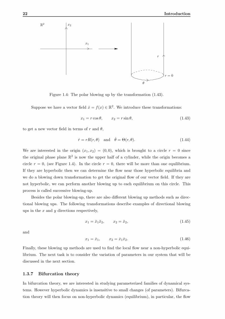
22 Introduction
r
θ
r = 0
x2
x1
R2
Figure 1.4: The polar blowing up by the transformation (1.43).
Suppose we have a vector field x = f(x) ∈ R2. We introduce these transformations:
x1 = r cos θ, x2 = r sin θ, (1.43)
to get a new vector field in terms of r and θ,
r = rR(r, θ) and θ = Θ(r, θ). (1.44)
We are interested in the origin (x1, x2) = (0, 0), which is brought to a circle r = 0 since
the original phase plane R2 is now the upper half of a cylinder, while the origin becomes a
circle r = 0, (see Figure 1.4). In the circle r = 0, there will be more than one equilibrium.
If they are hyperbolic then we can determine the flow near those hyperbolic equilibria and
we do a blowing down transformation to get the original flow of our vector field. If they are
not hyperbolic, we can perform another blowing up to each equilibrium on this circle. This
process is called successive blowing-up.
Besides the polar blowing-up, there are also different blowing up methods such as direc-
tional blowing ups. The following transformations describe examples of directional blowing
ups in the x and y directions respectively,
x1 = x1x2, x2 = x2, (1.45)
and
x1 = x1, x2 = x1x2. (1.46)
Finally, these blowing up methods are used to find the local flow near a non-hyperbolic equi-
librium. The next task is to consider the variation of parameters in our system that will be
discussed in the next section.
1.3.7 Bifurcation theory
In bifurcation theory, we are interested in studying parameterized families of dynamical sys-
tems. However hyperbolic dynamics is insensitive to small changes (of parameters). Bifurca-
tion theory will then focus on non-hyperbolic dynamics (equilibrium), in particular, the flow
1.3 Mathematical preliminaries 23
on the center manifold. When we want to study such a non-hyperbolic dynamical system,
we will vary some parameters. This process is called an “unfolding” of bifurcations. The
following questions are addressed.
1. What kind of local bifurcations do we typically have in dynamical systems with param-
eters?
2. Can we represent these local bifurcations by a normal form (simple model) with param-
eters?
3. If we vary some parameters of a particular dynamical system, will this dynamical system
display the same bifurcation?
The answers to the above questions have been long discussed by various people. We will not
go through the details, instead, we will summarize what has been done.
When a dynamical system has a degeneracy (i.e. a vector field has a non-hyperbolic
equilibrium) we can use the center manifold theorem and a normalization technique to simplify
the vector field locally. The local flow of such a degenerate vector field can also be determined
by a blowing-up technique. Then when this normal form is varied by a parameter (i.e. an
unfolding of bifurcation), we will have a bifurcation. How we vary parameters and what typical
bifurcations occur has already been derived. We summarize all common local bifurcations and
their unfolding of normal forms in the following.
1.3.7.1 Saddle-node bifurcation
Consider an autonomous dynamical system x = f(x, µ), x ∈ Rn, depending on one parameter
µ ∈ R, where f is smooth. Suppose at µ = 0 the vector field has the origin as the equilibrium
and the linearized matrix of the vector field evaluated at the origin, fx(0, 0), has a single zero
eigenvalue. Since the center manifold of this degeneracy is one-dimensional, we can reduce
the system to a one-dimensional vector field ˙x = f(x, µ), x, µ ∈ R1. Suppose the following
non-degeneracy conditions also hold:
1.df
dµ(0, 0) 6= 0, and
2.d2f
dx2(0, 0) 6= 0.
In Kuznetsov [78] the first condition above is called a transversality condition while the second
condition above is called a non-degeneracy condition. As µ passes through µ = 0, a saddle-
node bifurcation occurs. Moreover, the vector field is topologically equivalent near (0, 0) to
the following normal form,
y = α± y2, y, α ∈ R, (1.47)
at which two equilibria appear and vanish. Here, the normal form is one-dimensional as the
center manifold of the single zero eigenvalue degeneracy is one-dimensional. This bifurcation
is well known and all information about this bifurcation can be found in any bifurcation text
book [126].
24 Introduction
We remark that this bifurcation is codimension-one since there is only one degeneracy
which is the single zero eigenvalue. Generally, we only need one parameter in order to violate
this degeneracy. Therefore, a vector field is possible to undergo a codimension-one bifurcation
by varying only one parameter.
1.3.7.2 Transcritical bifurcation
Consider an autonomous dynamical system x = f(x, µ), x ∈ Rn, depending on one parameter
µ ∈ R, where f is smooth. Suppose at µ = 0 the vector field has the origin as an equilibrium
and the linearized matrix of the vector field evaluated at the origin, fx(0, 0), has a single zero
eigenvalue. As the center manifold is one-dimensional, we can reduce the system to a one-
dimensional vector field ˙x = f(x, µ), x, µ ∈ R1 and suppose the first non-degeneracy condition
in the saddle-node bifurcation is violated, i.e., dfdµ
(0, 0) = 0. Lastly, suppose the following
non-degeneracy conditions hold:
1.d2f
dxdµ(0, 0) 6= 0, and
2.d2f
dx2(0, 0) 6= 0.
Then as µ passes through µ = 0, a transcritical bifurcation occurs. Moreover, the vector field
is topologically equivalent near (0, 0) to the following normal form,
y = αy ± y2, y, α ∈ R, (1.48)
at which an equilibrium crosses another equilibrium and exchanges stabilities. Here, the
normal form is one-dimensional as the center manifold of the single zero eigenvalue degeneracy
is one-dimensional. This bifurcation is not a typical codimension-one bifurcation. It is mainly
because there are two degeneracy conditions we have to meet while there is only a single
parameter to vary. This bifurcation occurs mainly when one varies the parameter in such
a way that the non-degeneracy condition (of a saddle-node bifurcation) is violated. This
bifurcation might also occur in a system having a special structure so that we always have the
non-degeneracy condition violated.
1.3.7.3 Hopf bifurcation
Consider an autonomous dynamical system x = f(x, µ), x ∈ Rn, depending on one parameter
µ ∈ R, where f is smooth. Suppose the following conditions hold:
1. for all sufficiently small |µ| the system has a family of equilibria, x0(µ),
2. the first derivative of the vector field, fx(x0(µ), µ) has one pair of complex eigenvalues
λ(µ) = Re (λ(µ)) + iIm (λ(µ)),
that becomes purely imaginary when µ = 0, i.e., Re (λ(0)) = 0 and Im (λ(0)) = ω > 0.
Suppose the following non-degeneracy conditions also hold:
1.3 Mathematical preliminaries 25
1.dRe (λ)
dµ(0) 6= 0, and
2. l1(0) 6= 0.
Then as µ passes through µ = 0, a Hopf bifurcation occurs. Moreover, the vector field is
topologically equivalent near x0(0) to the following normal form,
y1 = αy1 − ωy2 + (ay1 − by2)(y21 + y2
2),
y2 = ωy1 + αy2 + (by1 + ay2)(y21 + y2
2).(1.49)
At which, α = 0, the equilibrium changes stability and a unique limit cycle bifurcates from
it. The function l1(µ) is called the Lyapunov coefficient. This can be obtained when one
computes the normal form of the vector field with a pair of purely imaginary eigenvalues. We
will not describe how to obtain the Lyapunov coefficient, instead we refer to Kuznetsov [80] for
more information how to compute this coefficient from the normal form derivation. Here, the
normal form is two-dimensional as the center manifold of this degeneracy is two-dimensional.
This bifurcation is also well known in the field of bifurcation theory. Remark that the Hopf
bifurcation is also codimension-one as there is only one degeneracy (i.e. a pair of purely
imaginary eigenvalues).
The saddle-node and Hopf bifurcations are known to be codimension-one bifurcations as
they have one degeneracy. Additional codimension-one bifurcations that a vector field could
undergo are pitchfork bifurcation (i.e. a single zero eigenvalue degeneracy in a vector field
with Z2 symmetry), homoclinic bifurcation (i.e. an occurrence of homolinic solutions) and
heteroclinic bifurcation (i.e. an occurrence of heteroclinic solution). More degeneracies that
could come from the lowest non-linear term in the normal form and the linear part of the vector
field could also occur. These give rise to more degenerate bifurcations, namely codimension
two bifurcations. These are common codimension two bifurcations; cusp, Bautin, Bogdanov-
Takens and fold-Hopf bifurcations. The unfoldings of such codimension two bifurcations have
also been studied. We can now say that if we perform an unfolding of a vector field and
we find these typical bifurcations (codimension-one and codimension two bifurcations) then
the unfolding is versal (or universal). One characteristic of a versal unfolding is when the
transformation that brings the parameter space of the original vector field to the parameter
space of the normal form is invertible.
This bifurcation analysis is usually represented by using a bifurcation diagram which plots
bifurcation conditions with respect to parameters that we vary. In the two-dimensional param-
eter space bifurcation set, a codimension-one bifurcation will be a curve, and a codimension-
two bifurcation will be a point, which is made up by an interaction of two or more codimension-
one bifurcation curves.
Up to this point, we have listed all typical bifurcations and we have confirmed that these
bifurcations can be represented by normal forms with their versal unfoldings. However, the
third question raised at the start of section 1.3.7 has not been completely solved. This is also
the question that we try to answer in this thesis.
26 Introduction
1.3.8 Additional notes to references
The history of dynamical systems goes back to three centuries ago when Euler attempted to
study the motion of the moon that is now so-called the N -body problem. Not only that, but
there are also a lot of other problems in science and engineering that can be modelled as a
dynamical system. To name a few, population dynamics, atmospheric models, the prediction
of stock market prices are among those problems. A revolutionary contribution to the theory
of dynamical systems is due to Henri Poincare. His proposal is to look at the geometry of
solutions instead of the explicit formula of solutions. For an introduction to the modern
theory of dynamical systems we refer to Katok and Hasselblatt [66]. For a mathematically
oriented approach to dynamical systems theory, we refer to Guckenheimer and Holmes [47]
and Wiggins [126]. The theory of center manifold and normalization technique are two of the
modern developments in the theory of dynamical systems. More information can be found in
Broer et al. [12]. Bifurcation theory is another subject in the modern theory of dynamical
systems which finds its origin in the work of Poincare. For a more practical approach to
bifurcation theory, we refer to Kuznetsov [78]. The blowing-up method is also one of the new
developments of the theory of dynamical systems, (see the paper by Takens [116]).
1.4 Outline of this thesis
Since this thesis is a collection of studies that analyse the Lotka-Volterra system with constant
terms, each chapter can be read separately. In chapter 2, we will discuss bifurcation analysis
of two-dimensional Lotka-Volterra systems with a constant term. It is shown that the Lotka-
Volterra system with a constant term undergoes a series of bifurcations when we vary the
constant term. Moreover, if we also vary another parameter, it is shown that more degenerate
bifurcations can occur. We show that these bifurcations are different from typical bifurcations
that we usually find in text books. In this chapter, we analyse those unusual degenerate
bifurcations, and explain how these bifurcation are created and unfolded in our system.
The analysis in chapter 2 does not deal with why these unusual bifurcations are there
in the first place. One of the reasons this happens is because of a special structure that is
possessed by our system. In chapter 3, we shall perform an analysis of a dynamical system that
possesses the same special structure as our system does, namely a codimension-one invariant
manifold that exists for every value of the parameters. We will perform a general global
bifurcation analysis on a general system with an invariant manifold and show that the system
with an invariant manifold will undergo a series of different bifurcations which do not normally
occur in a general system. We also show that the Lotka-Volterra system with a constant term
undergoes the same bifurcations that are found in this chapter.
In chapter 4, we discuss the existence of first integrals of dynamical systems, in particular
of two and three-dimensional Lotka-Volterra systems with constant terms. The existence of
first integrals of two and three-dimensional Lotka-Volterra equations has already attracted
much attention, however, we believe that the first integral of Lotka-Volterra systems with
constant terms has not been analysed. We will discuss the cases when all constant terms
1.4 Outline of this thesis 27
are not zero, at least one constant term is zero, respectively when all of the constant terms
are zero. The latter is included in our thesis in order to have a complete investigation of all
possible cases. It is shown that the Lotka-Volterra system with constant terms is integrable
for specific values of the parameters.
In chapter 5, a discussion of the major results presented in this thesis is given. We
discuss the common thread that connects all of our results together. We also discuss some
ideas and possible future projects we can pursue regarding results obtained in chapters 2, 3
and 4. Finally, an overall conclusion is given.

CHAPTER 2
Unusual bifurcations in theLotka-Volterra system with a
constant term
2.1 Introduction
Interactions between bifurcations of equilibria and of cycles (i.e. periodic orbits) occur nat-
urally in dynamical systems. In the bifurcation diagram, the interaction points often act as
organising centres, at which local and global bifurcations converge and the behaviour of the
system is determined to a large extent. These interaction points have been the subject of in-
tensive research over the last decades and, in particular, all interaction points which occur in
general dynamical systems have been classified and analysed in the literature, see for instance,
Kuznetsov [78].
However, the theory of interactions between bifurcations for systems with a special struc-
ture is, as yet, incomplete. In such systems, bifurcations can have a lower codimension than
that in the general case. For instance, the presence of a Z2 symmetry in the dynamical system
can render the pitchfork bifurcation codimension-one, whereas the number of degeneracies of
this bifurcation is the same as that of general codimension-two bifurcations. Pitchfork bifurca-
tions occur in particular in certain normal forms with a special structure namely S1 symmetry,
such as the saddle-node–Hopf normal form, after decoupling of the angular variable, see Guck-
enheimer and Holmes [47]. For this reason interactions with pitchfork bifurcations have been
extensively investigated. Here we mention a few contributions: Scheurle and Marsden [109]
discussed the existence of tori and quasiperiodic flows resulting from saddle-node–Hopf bifur-
cations, while Broer and Vegter [13] discussed the existence of Shilnikov bifurcations. The
existence of heteroclinic orbits was investigated by Lamb et al. [84] for the saddle-node–Hopf
system with time reversal symmetry and for the saddle-node–pitchfork system by Kirk and
Knobloch [70].
Interactions that involve a transcritical bifurcation, in contrast, have not attracted much
attention. This might be because this bifurcation does not correspond to a global phase space
symmetry, like the pitchfork bifurcation. However, the transcritical bifurcation is generic in
30 Unusual bifurcations in the Lotka-Volterra system with a constant term
dynamical systems in which an equilibrium must exist for all values of the parameters. An
example with this property comes from population dynamic models. In the Lotka-Volterra
type model, the variables are the population densities of several species. If a species dies out, it
cannot be regenerated and therefore the coordinate axes of such a model are invariant and the
origin is always an equilibrium solution (see, e.g. Zhu et al. [131]). In this current chapter, we
will investigate the interactions between saddle-node and transcritical bifurcations that occur
in the two-dimensional Lotka-Volterra system with a constant term. To our best knowledge,
this interaction has not been reported on in the literature before.
From a bifurcation theory point of view, the transcritical bifurcation can be considered
as a non-versal unfolding of the well-know saddle-node bifurcation. The normal form of the
saddle-node bifurcation is given by
x = µ+ x2,
while the normal form of the transcritical bifurcation is given by
y = αy + y2.
If we apply the transformation z = y + α2 to the system above we obtain
z = −α2
4+ z2,
which is a normal form of the saddle-node bifurcation parameterized by α. Thus, we can
consider the transcritical bifurcation as an unfolding of the saddle-node bifurcation. Because
the map µ = −α2/4 is noninvertible at the bifurcation point α = µ = 0, this unfolding is
non-versal.
Using the idea above, we investigate two different saddle-node–transcritical interactions,
which correspond to a single zero and a double zero eigenvalue degeneracy respectively. In
the former case, there is no additional bifurcation and the bifurcation diagram around the
interaction can be considered as a non-versal unfolding of the cusp bifurcation. The second
case is more complicated as the normal form of a double zero eigenvalue degeneracy is the
Bogdanov-Takens (BT) normal form. Due to nondegeneracy conditions of the transcritical
bifurcation, we obtain the normal form of a degenerate BT (DBT) bifurcation. Not only the
saddle-node and transcritical bifurcations are present, but there are also Hopf, homoclinic and
heteroclinic bifurcations appearing. We find two topologically different diagrams correspond-
ing to different unfoldings of the DBT singularity, namely, the elliptic and the saddle cases.
A complete topological classification of the DBT bifurcation has been analysed in Dumortier
et al. [31].
2.2 Bifurcation diagram of the Lotka-Volterra system with a
constant term
The two-dimensional Lotka-Volterra model with a constant term is given below,
x1 = x1(b1 + a11x1 + a12x2) + e,
x2 = x2(b2 + a21x1 + a22x2), (2.1)
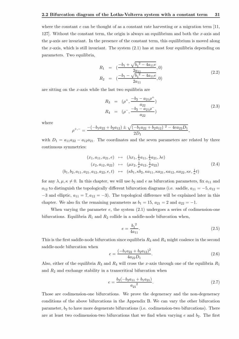
2.2 Bifurcation diagram of the Lotka-Volterra system with a constant term 31
where the constant e can be thought of as a constant rate harvesting or a migration term [11,
127]. Without the constant term, the origin is always an equilibrium and both the x-axis and
the y-axis are invariant. In the presence of the constant term, this equilibrium is moved along
the x-axis, which is still invariant. The system (2.1) has at most four equilibria depending on
parameters. Two equilibria,
R1 = (−b1 +
√
b 21 − 4a11e
2a11, 0)
R2 = (−b1 −
√
b 21 − 4a11e
2a11, 0)
(2.2)
are sitting on the x-axis while the last two equilibria are
R3 = (ρ+,−b2 − a21ρ
+
a22)
R4 = (ρ−,−b2 − a21ρ
−
a22)
(2.3)
where
ρ+,− =−(−b1a22 + b2a12) ±
√
(−b1a22 + b2a12) 2 − 4ea22D1
2D1,
with D1 = a11a22 − a12a21. The coordinates and the seven parameters are related by three
continuous symmetries:
(x1, a11, a21, e) 7→ (λx1,1λa11,
1λa21, λe)
(x2, a12, a22) 7→ (µx2,1µa12,
1µa22)
(b1, b2, a11, a21, a12, a22, e, t) 7→ (κb1, κb2, κa11, κa21, κa12, κa22, κe,1κt)
(2.4)
for any λ, µ, κ 6= 0. In this chapter, we will use b2 and e as bifurcation parameters, fix a11 and
a12 to distinguish the topologically different bifurcation diagrams (i.e. saddle, a11 = −5, a12 =
−3 and elliptic, a11 = 7, a12 = −3). The topological difference will be explained later in this
chapter. We also fix the remaining parameters as b1 = 15, a21 = 2 and a22 = −1.
When varying the parameter e, the system (2.1) undergoes a series of codimension-one
bifurcations. Equilibria R1 and R2 collide in a saddle-node bifurcation when,
e =b 21
4a11. (2.5)
This is the first saddle-node bifurcation since equilibria R3 and R4 might coalesce in the second
saddle-node bifurcation when
e =(−b1a22 + b2a12)2
4a22D1. (2.6)
Also, either of the equilibria R3 and R4 will cross the x-axis through one of the equilibria R1
and R2 and exchange stability in a transcritical bifurcation when
e =b2(−b2a11 + b1a21)
a 221
. (2.7)
Those are codimension-one bifurcations. We prove the degeneracy and the non-degeneracy
conditions of the above bifurcations in the Appendix B. We can vary the other bifurcation
parameter, b2 to have more degenerate bifurcations (i.e. codimension-two bifurcations). There
are at least two codimension-two bifurcations that we find when varying e and b2. The first
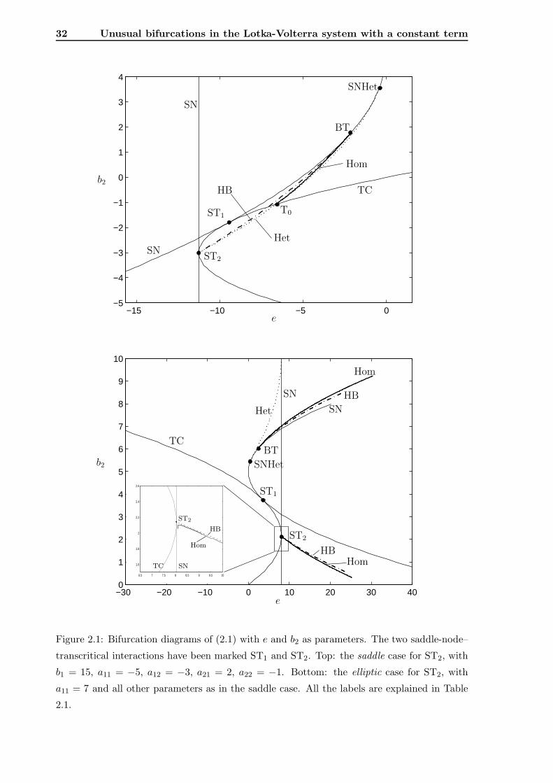
32 Unusual bifurcations in the Lotka-Volterra system with a constant term
−15 −10 −5 0−5
−4
−3
−2
−1
0
1
2
3
4
Hom
BT
SNHet
T0
b2
e
ST1
ST2
HB
SN
SN
TC
Het
−30 −20 −10 0 10 20 30 400
1
2
3
4
5
6
7
8
9
10
6.5 7 7.5 8 8.5 9 9.5 10
1.6
1.8
2
2.2
2.4
2.6
e
b2
TC
SN
ST1
SN
HBHom
HB
Hom
BT
SNHet
Het
ST2
TC SN
HB
HomST2
Figure 2.1: Bifurcation diagrams of (2.1) with e and b2 as parameters. The two saddle-node–
transcritical interactions have been marked ST1 and ST2. Top: the saddle case for ST2, with
b1 = 15, a11 = −5, a12 = −3, a21 = 2, a22 = −1. Bottom: the elliptic case for ST2, with
a11 = 7 and all other parameters as in the saddle case. All the labels are explained in Table
2.1.
2.2 Bifurcation diagram of the Lotka-Volterra system with a constant term 33
Symbols Bifurcations Codimension of bifurcation
BT Bogdanov-Takens 2
HB Hopf 1
Het Heteroclinic 1
Hom Homoclinic 1
SN Saddle-node 1
ST Saddle-node–transcritical 2
TC Transcritical 1
T0 Heteroclinic–homoclinic 2
Table 2.1: List of bifurcations that occur in the Lotka Volterra system with a constant term.
codimension-two bifurcation occurs when the system satisfies the conditions of the second
saddle-node bifurcation (2.6) and of the transcritical bifurcation (2.7), at which three equilibria
(R3, R4 and R1 ) collide. It turns out that if the parameters satisfy these conditions, the
linearized matrix of the system (2.1),
J(R1 = R3 = R4) =
−b1a12a21
D2−b1a12a22
D2
0 0
(2.8)
has a single-zero eigenvalue.
The second codimension-two bifurcation that we have found is when the parameters
satisfy conditions of the first saddle-node bifurcation (2.5) and of the transcritical bifurcation
(2.7), at which three equilibria (R1, R2 and R3) collide. The linearized matrix of the system
is,
J(R1 = R2 = R3) =
0 −b1a12
2a11
0 0
. (2.9)
In Figure 2.1 a complete bifurcation diagram is presented for two topologically different
cases. In each bifurcation diagram, there are two saddle-node bifurcations (labelled SN)
and one transcritical bifurcation (labelled TC). The first saddle-node bifurcation, which is
represented by a vertical line in both figures, is a collision between equilibria that lie on
the x-axis (R1 and R2). The other saddle-node bifurcation curve involves the other two
equilibria (R3 and R4). The transcritical bifurcation coincides with the second saddle-node
bifurcation to create the single zero eigenvalue degeneracy (labelled ST1), while the double
zero eigenvalue degeneracy (labelled ST2) is created from the interaction of the transcritical
bifurcation with the first saddle-node bifurcation. Additional codimension-one bifurcations
also appear such as a Hopf bifurcation curve (labelled HB), heteroclinic connections (labelled
Het) and homoclinic loops (labelled Hom). Unlike saddle-node and transcritical bifurcation,
which are obtained analytically, these additional bifurcations are detected numerically by
a continuation software package for dynamical systems, namely AUTO2000 (see Doedel et
al. [29]). Continuing further those codimension-one bifurcation curves we obtain codimension-
two bifurcation points such as a Bogdanov-Takens (BT), saddle-node/heteroclinic bifurcation
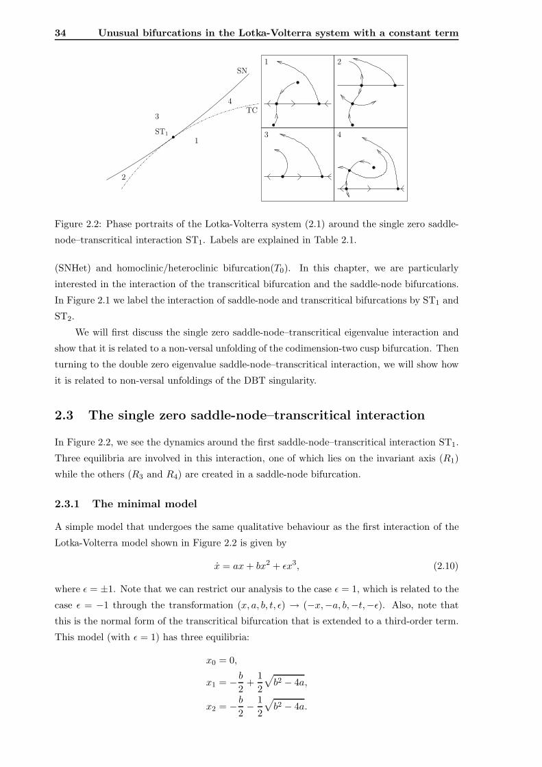
34 Unusual bifurcations in the Lotka-Volterra system with a constant term
1 2
3 4
3
SN
TC4
2
1ST1
Figure 2.2: Phase portraits of the Lotka-Volterra system (2.1) around the single zero saddle-
node–transcritical interaction ST1. Labels are explained in Table 2.1.
(SNHet) and homoclinic/heteroclinic bifurcation(T0). In this chapter, we are particularly
interested in the interaction of the transcritical bifurcation and the saddle-node bifurcations.
In Figure 2.1 we label the interaction of saddle-node and transcritical bifurcations by ST1 and
ST2.
We will first discuss the single zero saddle-node–transcritical eigenvalue interaction and
show that it is related to a non-versal unfolding of the codimension-two cusp bifurcation. Then
turning to the double zero eigenvalue saddle-node–transcritical interaction, we will show how
it is related to non-versal unfoldings of the DBT singularity.
2.3 The single zero saddle-node–transcritical interaction
In Figure 2.2, we see the dynamics around the first saddle-node–transcritical interaction ST1.
Three equilibria are involved in this interaction, one of which lies on the invariant axis (R1)
while the others (R3 and R4) are created in a saddle-node bifurcation.
2.3.1 The minimal model
A simple model that undergoes the same qualitative behaviour as the first interaction of the
Lotka-Volterra model shown in Figure 2.2 is given by
x = ax+ bx2 + ǫx3, (2.10)
where ǫ = ±1. Note that we can restrict our analysis to the case ǫ = 1, which is related to the
case ǫ = −1 through the transformation (x, a, b, t, ǫ) → (−x,−a, b,−t,−ǫ). Also, note that
this is the normal form of the transcritical bifurcation that is extended to a third-order term.
This model (with ǫ = 1) has three equilibria:
x0 = 0,
x1 = − b2
+1
2
√
b2 − 4a,
x2 = − b2− 1
2
√
b2 − 4a.
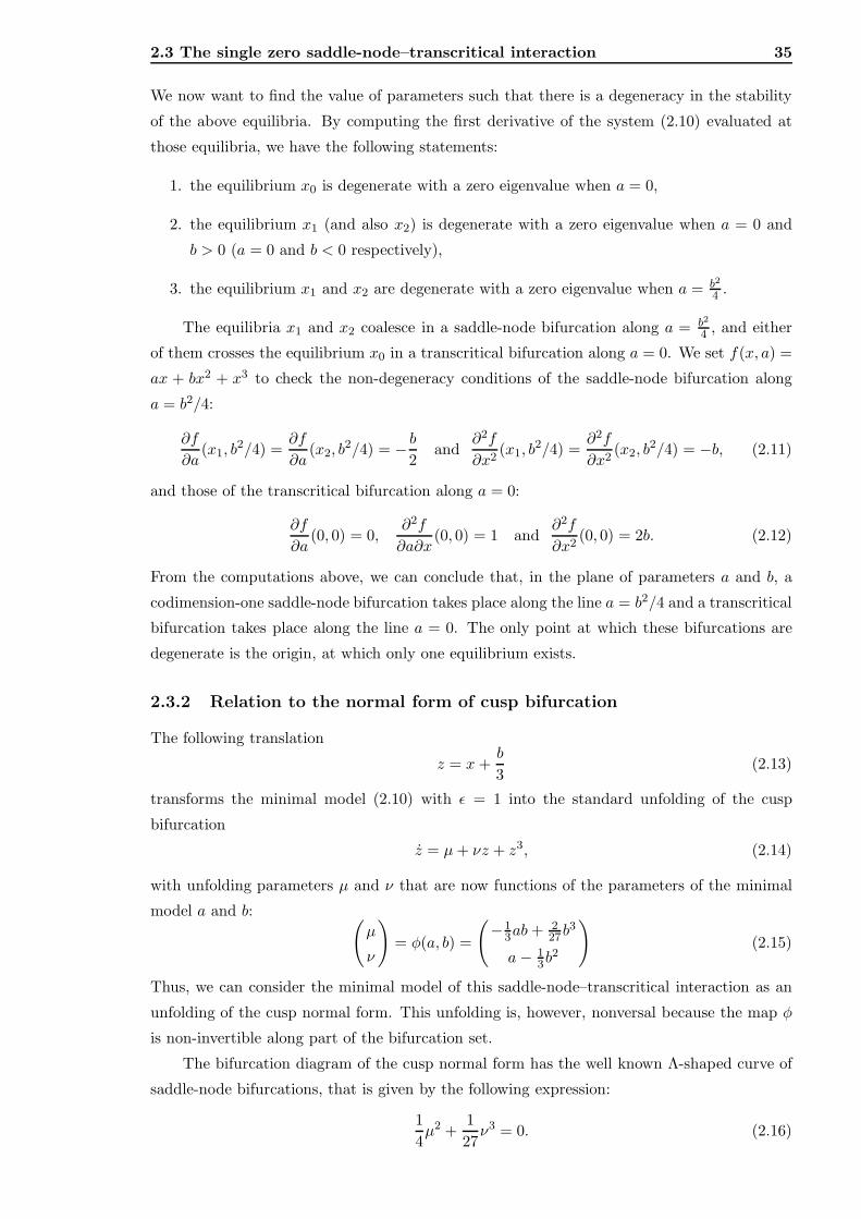
2.3 The single zero saddle-node–transcritical interaction 35
We now want to find the value of parameters such that there is a degeneracy in the stability
of the above equilibria. By computing the first derivative of the system (2.10) evaluated at
those equilibria, we have the following statements:
1. the equilibrium x0 is degenerate with a zero eigenvalue when a = 0,
2. the equilibrium x1 (and also x2) is degenerate with a zero eigenvalue when a = 0 and
b > 0 (a = 0 and b < 0 respectively),
3. the equilibrium x1 and x2 are degenerate with a zero eigenvalue when a = b2
4 .
The equilibria x1 and x2 coalesce in a saddle-node bifurcation along a = b2
4 , and either
of them crosses the equilibrium x0 in a transcritical bifurcation along a = 0. We set f(x, a) =
ax + bx2 + x3 to check the non-degeneracy conditions of the saddle-node bifurcation along
a = b2/4:
∂f
∂a(x1, b
2/4) =∂f
∂a(x2, b
2/4) = − b2
and∂2f
∂x2(x1, b
2/4) =∂2f
∂x2(x2, b
2/4) = −b, (2.11)
and those of the transcritical bifurcation along a = 0:
∂f
∂a(0, 0) = 0,
∂2f
∂a∂x(0, 0) = 1 and
∂2f
∂x2(0, 0) = 2b. (2.12)
From the computations above, we can conclude that, in the plane of parameters a and b, a
codimension-one saddle-node bifurcation takes place along the line a = b2/4 and a transcritical
bifurcation takes place along the line a = 0. The only point at which these bifurcations are
degenerate is the origin, at which only one equilibrium exists.
2.3.2 Relation to the normal form of cusp bifurcation
The following translation
z = x+b
3(2.13)
transforms the minimal model (2.10) with ǫ = 1 into the standard unfolding of the cusp
bifurcation
z = µ+ νz + z3, (2.14)
with unfolding parameters µ and ν that are now functions of the parameters of the minimal
model a and b:(
µ
ν
)
= φ(a, b) =
(
−13ab+ 2
27b3
a− 13b
2
)
(2.15)
Thus, we can consider the minimal model of this saddle-node–transcritical interaction as an
unfolding of the cusp normal form. This unfolding is, however, nonversal because the map φ
is non-invertible along part of the bifurcation set.
The bifurcation diagram of the cusp normal form has the well known Λ-shaped curve of
saddle-node bifurcations, that is given by the following expression:
1
4µ2 +
1
27ν3 = 0. (2.16)
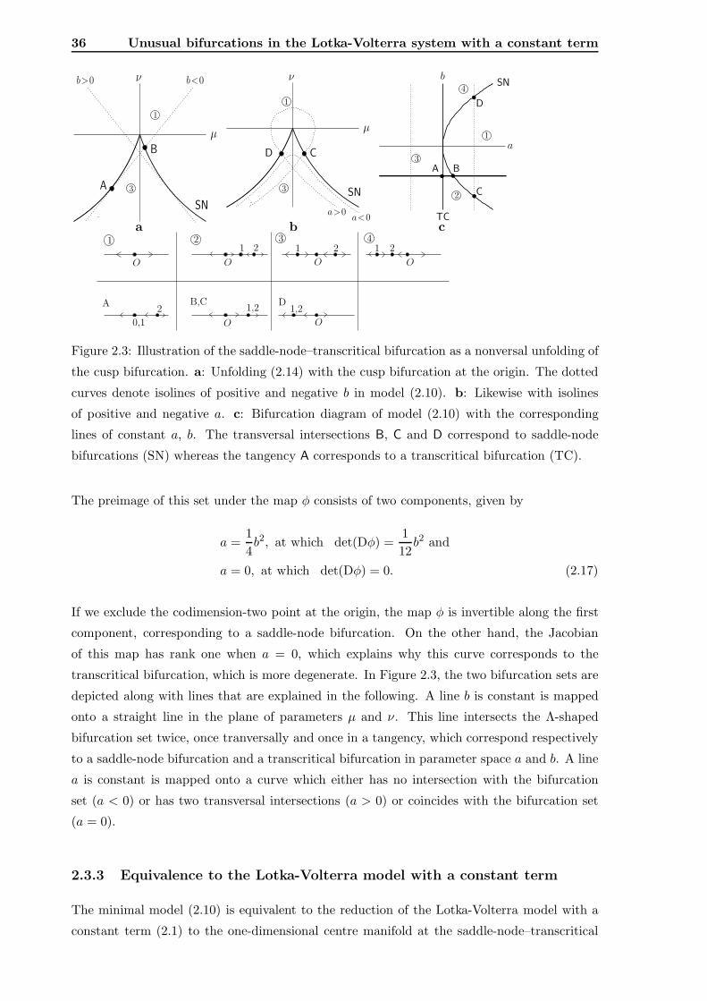
36 Unusual bifurcations in the Lotka-Volterra system with a constant term
ν
µ
SN
A
B
b>0 b<0
1
3
ν
µ
SN
D
a>0a<0
C
1
3
a
SN
C
D
BA
TC
b
1
2
3
4
a b c
O
1 2
O
1 2
O
1 2
O
O
1,2
0,1
2
O
1,2
1 2 3 4
A B,C D
Figure 2.3: Illustration of the saddle-node–transcritical bifurcation as a nonversal unfolding of
the cusp bifurcation. a: Unfolding (2.14) with the cusp bifurcation at the origin. The dotted
curves denote isolines of positive and negative b in model (2.10). b: Likewise with isolines
of positive and negative a. c: Bifurcation diagram of model (2.10) with the corresponding
lines of constant a, b. The transversal intersections B, C and D correspond to saddle-node
bifurcations (SN) whereas the tangency A corresponds to a transcritical bifurcation (TC).
The preimage of this set under the map φ consists of two components, given by
a =1
4b2, at which det(Dφ) =
1
12b2 and
a = 0, at which det(Dφ) = 0. (2.17)
If we exclude the codimension-two point at the origin, the map φ is invertible along the first
component, corresponding to a saddle-node bifurcation. On the other hand, the Jacobian
of this map has rank one when a = 0, which explains why this curve corresponds to the
transcritical bifurcation, which is more degenerate. In Figure 2.3, the two bifurcation sets are
depicted along with lines that are explained in the following. A line b is constant is mapped
onto a straight line in the plane of parameters µ and ν. This line intersects the Λ-shaped
bifurcation set twice, once tranversally and once in a tangency, which correspond respectively
to a saddle-node bifurcation and a transcritical bifurcation in parameter space a and b. A line
a is constant is mapped onto a curve which either has no intersection with the bifurcation
set (a < 0) or has two transversal intersections (a > 0) or coincides with the bifurcation set
(a = 0).
2.3.3 Equivalence to the Lotka-Volterra model with a constant term
The minimal model (2.10) is equivalent to the reduction of the Lotka-Volterra model with a
constant term (2.1) to the one-dimensional centre manifold at the saddle-node–transcritical
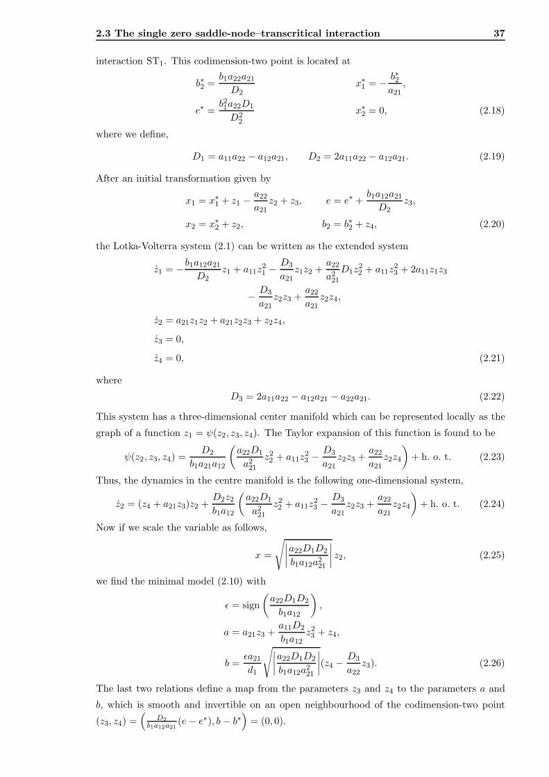
2.3 The single zero saddle-node–transcritical interaction 37
interaction ST1. This codimension-two point is located at
b∗2 =b1a22a21
D2x∗1 = − b∗2
a21,
e∗ =b21a22D1
D22
x∗2 = 0, (2.18)
where we define,
D1 = a11a22 − a12a21, D2 = 2a11a22 − a12a21. (2.19)
After an initial transformation given by
x1 = x∗1 + z1 −a22
a21z2 + z3, e = e∗ +
b1a12a21
D2z3,
x2 = x∗2 + z2, b2 = b∗2 + z4, (2.20)
the Lotka-Volterra system (2.1) can be written as the extended system
z1 = −b1a12a21
D2z1 + a11z
21 − D3
a21z1z2 +
a22
a221
D1z22 + a11z
23 + 2a11z1z3
− D3
a21z2z3 +
a22
a21z2z4,
z2 = a21z1z2 + a21z2z3 + z2z4,
z3 = 0,
z4 = 0, (2.21)
where
D3 = 2a11a22 − a12a21 − a22a21. (2.22)
This system has a three-dimensional center manifold which can be represented locally as the
graph of a function z1 = ψ(z2, z3, z4). The Taylor expansion of this function is found to be
ψ(z2, z3, z4) =D2
b1a21a12
(
a22D1
a221
z22 + a11z
23 − D3
a21z2z3 +
a22
a21z2z4
)
+ h. o. t. (2.23)
Thus, the dynamics in the centre manifold is the following one-dimensional system,
z2 = (z4 + a21z3)z2 +D2z2b1a12
(
a22D1
a221
z22 + a11z
23 − D3
a21z2z3 +
a22
a21z2z4
)
+ h. o. t. (2.24)
Now if we scale the variable as follows,
x =
√
∣
∣
∣
∣
a22D1D2
b1a12a221
∣
∣
∣
∣
z2, (2.25)
we find the minimal model (2.10) with
ǫ = sign
(
a22D1D2
b1a12
)
,
a = a21z3 +a11D2
b1a12z23 + z4,
b =ǫa21
d1
√
∣
∣
∣
∣
a22D1D2
b1a12a221
∣
∣
∣
∣
(z4 −D3
a22z3). (2.26)
The last two relations define a map from the parameters z3 and z4 to the parameters a and
b, which is smooth and invertible on an open neighbourhood of the codimension-two point
(z3, z4) =(
D2
b1a12a21(e− e∗), b− b∗
)
= (0, 0).
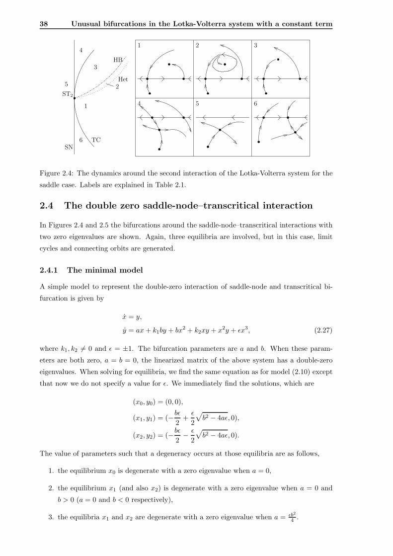
38 Unusual bifurcations in the Lotka-Volterra system with a constant term
4 5 6
1 2 3
1
6SN
2
3HB
Het
4
5
TC
ST2
Figure 2.4: The dynamics around the second interaction of the Lotka-Volterra system for the
saddle case. Labels are explained in Table 2.1.
2.4 The double zero saddle-node–transcritical interaction
In Figures 2.4 and 2.5 the bifurcations around the saddle-node–transcritical interactions with
two zero eigenvalues are shown. Again, three equilibria are involved, but in this case, limit
cycles and connecting orbits are generated.
2.4.1 The minimal model
A simple model to represent the double-zero interaction of saddle-node and transcritical bi-
furcation is given by
x = y,
y = ax+ k1by + bx2 + k2xy + x2y + ǫx3, (2.27)
where k1, k2 6= 0 and ǫ = ±1. The bifurcation parameters are a and b. When these param-
eters are both zero, a = b = 0, the linearized matrix of the above system has a double-zero
eigenvalues. When solving for equilibria, we find the same equation as for model (2.10) except
that now we do not specify a value for ǫ. We immediately find the solutions, which are
(x0, y0) = (0, 0),
(x1, y1) = (−bǫ2
+ǫ
2
√
b2 − 4aǫ, 0),
(x2, y2) = (−bǫ2
− ǫ
2
√
b2 − 4aǫ, 0).
The value of parameters such that a degeneracy occurs at those equilibria are as follows,
1. the equilibrium x0 is degenerate with a zero eigenvalue when a = 0,
2. the equilibrium x1 (and also x2) is degenerate with a zero eigenvalue when a = 0 and
b > 0 (a = 0 and b < 0 respectively),
3. the equilibria x1 and x2 are degenerate with a zero eigenvalue when a = ǫb2
4 .
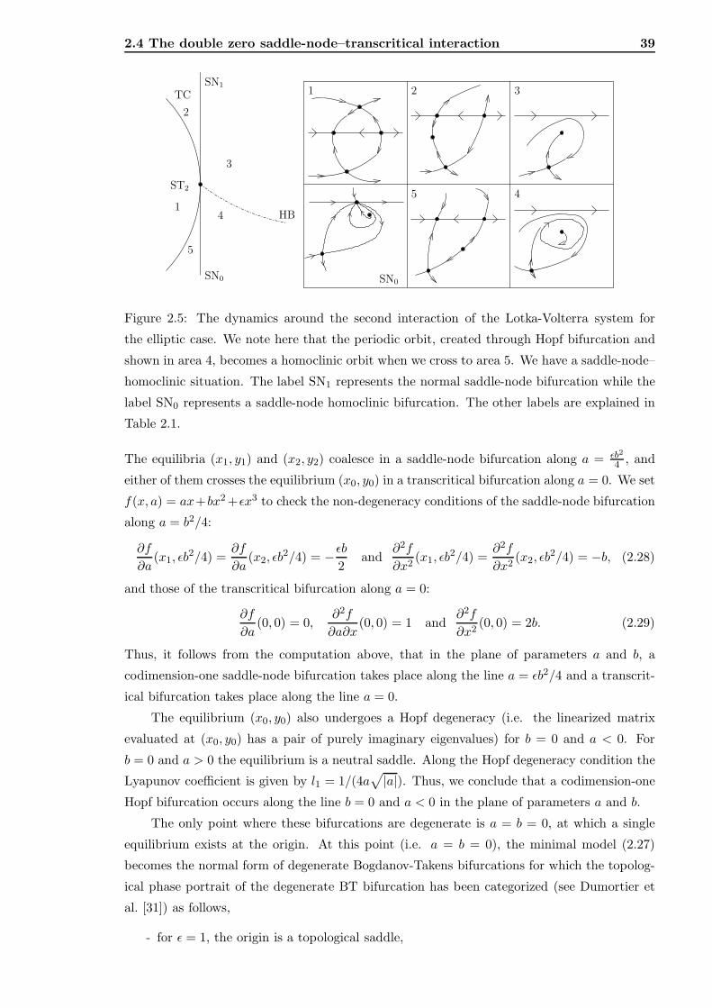
2.4 The double zero saddle-node–transcritical interaction 39
1
SN0
4
2
5
3
1
3
TC
2
ST2
5
4 HB
SN0
SN1
Figure 2.5: The dynamics around the second interaction of the Lotka-Volterra system for
the elliptic case. We note here that the periodic orbit, created through Hopf bifurcation and
shown in area 4, becomes a homoclinic orbit when we cross to area 5. We have a saddle-node–
homoclinic situation. The label SN1 represents the normal saddle-node bifurcation while the
label SN0 represents a saddle-node homoclinic bifurcation. The other labels are explained in
Table 2.1.
The equilibria (x1, y1) and (x2, y2) coalesce in a saddle-node bifurcation along a = ǫb2
4 , and
either of them crosses the equilibrium (x0, y0) in a transcritical bifurcation along a = 0. We set
f(x, a) = ax+bx2 +ǫx3 to check the non-degeneracy conditions of the saddle-node bifurcation
along a = b2/4:
∂f
∂a(x1, ǫb
2/4) =∂f
∂a(x2, ǫb
2/4) = −ǫb2
and∂2f
∂x2(x1, ǫb
2/4) =∂2f
∂x2(x2, ǫb
2/4) = −b, (2.28)
and those of the transcritical bifurcation along a = 0:
∂f
∂a(0, 0) = 0,
∂2f
∂a∂x(0, 0) = 1 and
∂2f
∂x2(0, 0) = 2b. (2.29)
Thus, it follows from the computation above, that in the plane of parameters a and b, a
codimension-one saddle-node bifurcation takes place along the line a = ǫb2/4 and a transcrit-
ical bifurcation takes place along the line a = 0.
The equilibrium (x0, y0) also undergoes a Hopf degeneracy (i.e. the linearized matrix
evaluated at (x0, y0) has a pair of purely imaginary eigenvalues) for b = 0 and a < 0. For
b = 0 and a > 0 the equilibrium is a neutral saddle. Along the Hopf degeneracy condition the
Lyapunov coefficient is given by l1 = 1/(4a√
|a|). Thus, we conclude that a codimension-one
Hopf bifurcation occurs along the line b = 0 and a < 0 in the plane of parameters a and b.
The only point where these bifurcations are degenerate is a = b = 0, at which a single
equilibrium exists at the origin. At this point (i.e. a = b = 0), the minimal model (2.27)
becomes the normal form of degenerate Bogdanov-Takens bifurcations for which the topolog-
ical phase portrait of the degenerate BT bifurcation has been categorized (see Dumortier et
al. [31]) as follows,
- for ǫ = 1, the origin is a topological saddle,
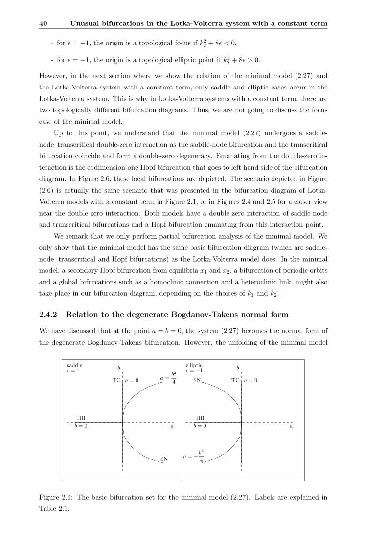
40 Unusual bifurcations in the Lotka-Volterra system with a constant term
- for ǫ = −1, the origin is a topological focus if k22 + 8ǫ < 0,
- for ǫ = −1, the origin is a topological elliptic point if k22 + 8ǫ > 0.
However, in the next section where we show the relation of the minimal model (2.27) and
the Lotka-Volterra system with a constant term, only saddle and elliptic cases occur in the
Lotka-Volterra system. This is why in Lotka-Volterra systems with a constant term, there are
two topologically different bifurcation diagrams. Thus, we are not going to discuss the focus
case of the minimal model.
Up to this point, we understand that the minimal model (2.27) undergoes a saddle-
node–transcritical double-zero interaction as the saddle-node bifurcation and the transcritical
bifurcation coincide and form a double-zero degeneracy. Emanating from the double-zero in-
teraction is the codimension-one Hopf bifurcation that goes to left hand side of the bifurcation
diagram. In Figure 2.6, these local bifurcations are depicted. The scenario depicted in Figure
(2.6) is actually the same scenario that was presented in the bifurcation diagram of Lotka-
Volterra models with a constant term in Figure 2.1, or in Figures 2.4 and 2.5 for a closer view
near the double-zero interaction. Both models have a double-zero interaction of saddle-node
and transcritical bifurcations and a Hopf bifurcation emanating from this interaction point.
We remark that we only perform partial bifurcation analysis of the minimal model. We
only show that the minimal model has the same basic bifurcation diagram (which are saddle-
node, transcritical and Hopf bifurcations) as the Lotka-Volterra model does. In the minimal
model, a secondary Hopf bifurcation from equilibria x1 and x2, a bifurcation of periodic orbits
and a global bifurcations such as a homoclinic connection and a heteroclinic link, might also
take place in our bifurcation diagram, depending on the choices of k1 and k2.
2.4.2 Relation to the degenerate Bogdanov-Takens normal form
We have discussed that at the point a = b = 0, the system (2.27) becomes the normal form of
the degenerate Bogdanov-Takens bifurcation. However, the unfolding of the minimal model
a = 0
b = 0 a
b
TC
SN
a = 0
b = 0 a
b
TCSNa =b2
4
a = −b2
4
saddle ellipticǫ = 1 ǫ = −1
HB HB
Figure 2.6: The basic bifurcation set for the minimal model (2.27). Labels are explained in
Table 2.1.
2.4 The double zero saddle-node–transcritical interaction 41
(2.27) can also be transformed into the unfolding of the codimension-three Bogdanov-Takens
bifurcation. The transformation
z1 = x+ǫ
3b− 2ǫ
3k2xb− ǫ
27k1b2,
z2 = y − 2ǫ
3k2by,
a = a− ǫ
3b2,
b = b− 1
9k1b2, (2.30)
brings the minimal model in the form of the standard unfolding of the degenerate Bogdanov-
Takens bifurcation, truncated up to terms of order three:
z1 = z2,
z2 = µ1 + µ2z1 + νz2 + k2z1z2 + z21z2 + ǫz3
1 , (2.31)
where
µ1 = − ǫ3
(
a+ǫ
9b2)
b,
µ2 = a,
ν =(
k1 −ǫ
3k2
)
b. (2.32)
The local partial bifurcation diagram of the normal form of the degenerate Bogdanov-Takens
bifurcation (2.31) is schematically depicted in Figure 2.7. The codimension-one saddle-node
bifurcation (labelled SN) and the codimension-one Hopf bifurcation (labelled HB) are now
surfaces in the three-dimensional space of parameters µ1, µ2 and ν. Equations, used to draw
saddle-node and Hopf bifurcation surfaces are:
27µ21 + 4ǫµ3
2 = 0,
and
µ21 + 3ǫk2µ1ν − k2µ1µ2 + ǫk2
2µ2ν − ǫk32µ1 + µ2
2ν − 2ǫµ2ν2 + ν3 = 0
respectively. The former equation is derived from solving the equation to find equilibria of the
system (2.31) and the condition such that the Jacobian matrix evaluated as those equilibria
has a single zero eigenvalue. While, the latter equation is derived from solving the equation
to find equilibria of the system (2.31) and the condition such that the trace of the Jacobian
matrix evaluated as those equilibria is zero.
The codimension-two Bogdanov-Takens bifurcation (labelled BT) is now a curve that
is formed from the interaction of the saddle-node and the Hopf bifurcation surfaces. The
degenerate Bogdanov-Takens bifurcation (labelled BT3) which is codimension-three, is the
origin of this parameter space. We note that this bifurcation set is partial. We do not draw
the complete bifurcation diagram since our main interest is to show the relation between
the minimal model and the normal form of codimension-three BT, especially the non-versal
unfolding of saddle-node–transcritical interaction.
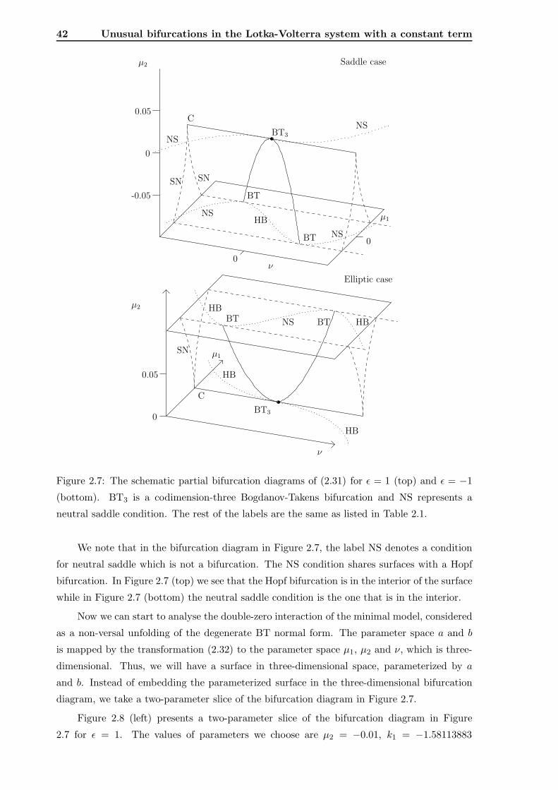
42 Unusual bifurcations in the Lotka-Volterra system with a constant term
0
0.05
µ2
ν
NS
BT3
SN
HB
HB
HB
HBBT BT
C
µ1
-0.05
0
0.05
0
0
µ2
µ1
ν
HB
BT
BT
BT3
SN SN
C
NS
NS
NS
NS
Saddle case
Elliptic case
Figure 2.7: The schematic partial bifurcation diagrams of (2.31) for ǫ = 1 (top) and ǫ = −1
(bottom). BT3 is a codimension-three Bogdanov-Takens bifurcation and NS represents a
neutral saddle condition. The rest of the labels are the same as listed in Table 2.1.
We note that in the bifurcation diagram in Figure 2.7, the label NS denotes a condition
for neutral saddle which is not a bifurcation. The NS condition shares surfaces with a Hopf
bifurcation. In Figure 2.7 (top) we see that the Hopf bifurcation is in the interior of the surface
while in Figure 2.7 (bottom) the neutral saddle condition is the one that is in the interior.
Now we can start to analyse the double-zero interaction of the minimal model, considered
as a non-versal unfolding of the degenerate BT normal form. The parameter space a and b
is mapped by the transformation (2.32) to the parameter space µ1, µ2 and ν, which is three-
dimensional. Thus, we will have a surface in three-dimensional space, parameterized by a
and b. Instead of embedding the parameterized surface in the three-dimensional bifurcation
diagram, we take a two-parameter slice of the bifurcation diagram in Figure 2.7.
Figure 2.8 (left) presents a two-parameter slice of the bifurcation diagram in Figure
2.7 for ǫ = 1. The values of parameters we choose are µ2 = −0.01, k1 = −1.58113883
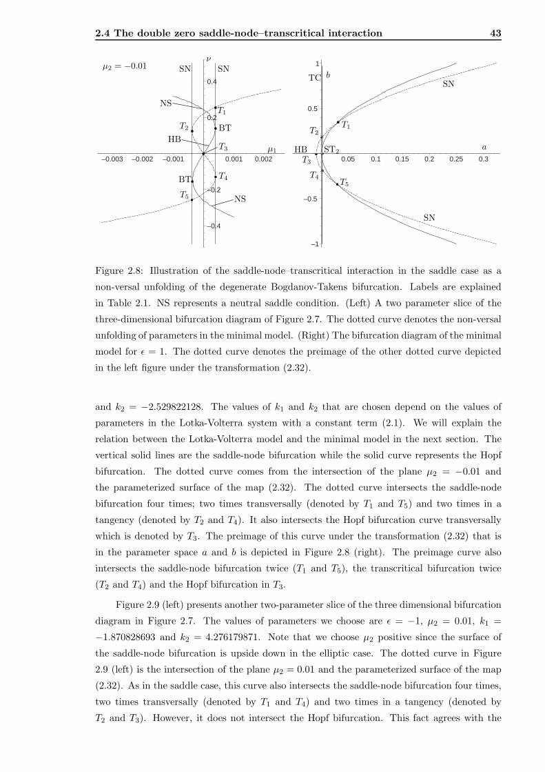
2.4 The double zero saddle-node–transcritical interaction 43
–0.4
–0.2
0.2
0.4
–0.003 –0.002 –0.001 0.001 0.002
–1
–0.5
0.5
1
b
0.05 0.1 0.15 0.2 0.25 0.3
a
a
NS
BT
T1
T3
T4
SN
b
T1
T5
µ1
NS
SN SN
νµ2 = −0.01
T3
SN
T2
HB
T5
BT
HB
TC
T2
T4
ST2
Figure 2.8: Illustration of the saddle-node–transcritical interaction in the saddle case as a
non-versal unfolding of the degenerate Bogdanov-Takens bifurcation. Labels are explained
in Table 2.1. NS represents a neutral saddle condition. (Left) A two parameter slice of the
three-dimensional bifurcation diagram of Figure 2.7. The dotted curve denotes the non-versal
unfolding of parameters in the minimal model. (Right) The bifurcation diagram of the minimal
model for ǫ = 1. The dotted curve denotes the preimage of the other dotted curve depicted
in the left figure under the transformation (2.32).
and k2 = −2.529822128. The values of k1 and k2 that are chosen depend on the values of
parameters in the Lotka-Volterra system with a constant term (2.1). We will explain the
relation between the Lotka-Volterra model and the minimal model in the next section. The
vertical solid lines are the saddle-node bifurcation while the solid curve represents the Hopf
bifurcation. The dotted curve comes from the intersection of the plane µ2 = −0.01 and
the parameterized surface of the map (2.32). The dotted curve intersects the saddle-node
bifurcation four times; two times transversally (denoted by T1 and T5) and two times in a
tangency (denoted by T2 and T4). It also intersects the Hopf bifurcation curve transversally
which is denoted by T3. The preimage of this curve under the transformation (2.32) that is
in the parameter space a and b is depicted in Figure 2.8 (right). The preimage curve also
intersects the saddle-node bifurcation twice (T1 and T5), the transcritical bifurcation twice
(T2 and T4) and the Hopf bifurcation in T3.
Figure 2.9 (left) presents another two-parameter slice of the three dimensional bifurcation
diagram in Figure 2.7. The values of parameters we choose are ǫ = −1, µ2 = 0.01, k1 =
−1.870828693 and k2 = 4.276179871. Note that we choose µ2 positive since the surface of
the saddle-node bifurcation is upside down in the elliptic case. The dotted curve in Figure
2.9 (left) is the intersection of the plane µ2 = 0.01 and the parameterized surface of the map
(2.32). As in the saddle case, this curve also intersects the saddle-node bifurcation four times,
two times transversally (denoted by T1 and T4) and two times in a tangency (denoted by
T2 and T3). However, it does not intersect the Hopf bifurcation. This fact agrees with the
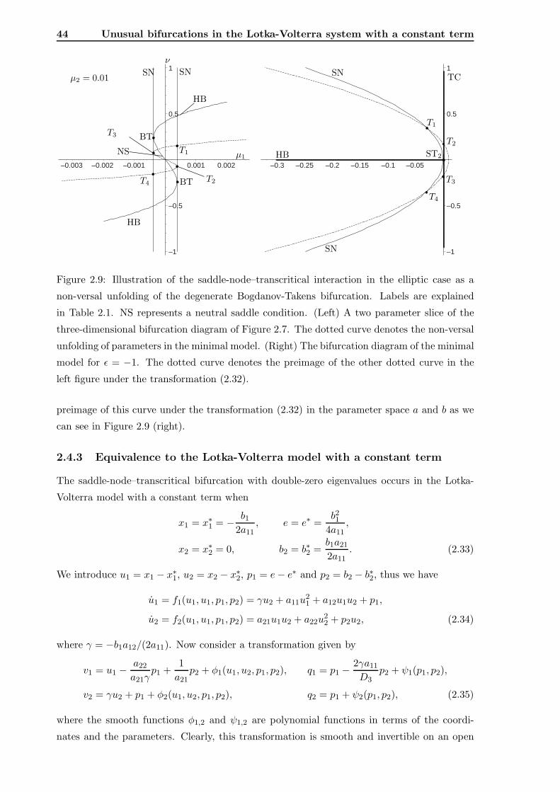
44 Unusual bifurcations in the Lotka-Volterra system with a constant term
–1
–0.5
0.5
1
–0.003 –0.002 –0.001 0.001 0.002
–1
–0.5
0.5
1
b
–0.3 –0.25 –0.2 –0.15 –0.1 –0.05
a
BT
BT
HB
HB
NS
SN SN
ν
µ1
T1
T2
T3
T4
SN
SN
HB
TC
T1
T4T2
T3
ST2
µ2 = 0.01
Figure 2.9: Illustration of the saddle-node–transcritical interaction in the elliptic case as a
non-versal unfolding of the degenerate Bogdanov-Takens bifurcation. Labels are explained
in Table 2.1. NS represents a neutral saddle condition. (Left) A two parameter slice of the
three-dimensional bifurcation diagram of Figure 2.7. The dotted curve denotes the non-versal
unfolding of parameters in the minimal model. (Right) The bifurcation diagram of the minimal
model for ǫ = −1. The dotted curve denotes the preimage of the other dotted curve in the
left figure under the transformation (2.32).
preimage of this curve under the transformation (2.32) in the parameter space a and b as we
can see in Figure 2.9 (right).
2.4.3 Equivalence to the Lotka-Volterra model with a constant term
The saddle-node–transcritical bifurcation with double-zero eigenvalues occurs in the Lotka-
Volterra model with a constant term when
x1 = x∗1 = − b12a11
, e = e∗ =b21
4a11,
x2 = x∗2 = 0, b2 = b∗2 =b1a21
2a11. (2.33)
We introduce u1 = x1 − x∗1, u2 = x2 − x∗2, p1 = e− e∗ and p2 = b2 − b∗2, thus we have
u1 = f1(u1, u1, p1, p2) = γu2 + a11u21 + a12u1u2 + p1,
u2 = f2(u1, u1, p1, p2) = a21u1u2 + a22u22 + p2u2, (2.34)
where γ = −b1a12/(2a11). Now consider a transformation given by
v1 = u1 −a22
a21γp1 +
1
a21p2 + φ1(u1, u2, p1, p2), q1 = p1 −
2γa11
D3p2 + ψ1(p1, p2),
v2 = γu2 + p1 + φ2(u1, u2, p1, p2), q2 = p1 + ψ2(p1, p2), (2.35)
where the smooth functions φ1,2 and ψ1,2 are polynomial functions in terms of the coordi-
nates and the parameters. Clearly, this transformation is smooth and invertible on an open
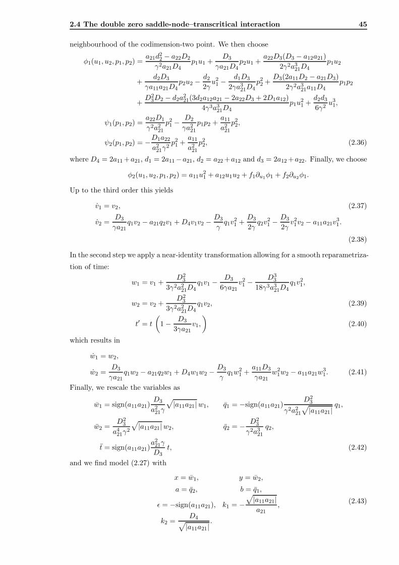
2.4 The double zero saddle-node–transcritical interaction 45
neighbourhood of the codimension-two point. We then choose
φ1(u1, u2, p1, p2) =a21d
22 − a22D2
γ2a21D4p1u1 +
D3
γa21D4p2u1 +
a22D3(D3 − a12a21)
2γ2a321D4
p1u2
+d2D3
γa11a21D4p2u2 −
d2
2γu2
1 −d1D3
2γa321D4
p22 +
D3(2a11D2 − a21D3)
2γ2a321a11D4
p1p2
+D2
3D2 − d2a221(3d2a12a21 − 2a22D3 + 2D1a12)
4γ3a321D4
p1u21 +
d2d3
6γ2u3
1,
ψ1(p1, p2) =a22D1
γ2a221
p21 −
D2
γa221
p1p2 +a11
a221
p22,
ψ2(p1, p2) = −D1a22
a221γ
2p21 +
a11
a221
p22, (2.36)
where D4 = 2a11 +a21, d1 = 2a11−a21, d2 = a22 +a12 and d3 = 2a12 +a22. Finally, we choose
φ2(u1, u2, p1, p2) = a11u21 + a12u1u2 + f1∂u1
φ1 + f2∂u2φ1.
Up to the third order this yields
v1 = v2, (2.37)
v2 =D3
γa21q1v2 − a21q2v1 +D4v1v2 −
D3
γq1v
21 +
D3
2γq2v
21 − D3
2γv21v2 − a11a21v
31 .
(2.38)
In the second step we apply a near-identity transformation allowing for a smooth reparametriza-
tion of time:
w1 = v1 +D2
3
3γ2a221D4
q1v1 −D3
6γa21v21 − D3
3
18γ3a321D4
q1v21,
w2 = v2 +D2
3
3γ2a221D4
q1v2, (2.39)
t′ = t
(
1 − D3
3γa21v1,
)
(2.40)
which results in
w1 = w2,
w2 =D3
γa21q1w2 − a21q2w1 +D4w1w2 −
D3
γq1w
21 +
a11D3
γa21w2
1w2 − a11a21w31. (2.41)
Finally, we rescale the variables as
w1 = sign(a11a21)D3
a221γ
√
|a11a21|w1, q1 = −sign(a11a21)D2
3
γ2a221
√
|a11a21|q1,
w2 =D2
3
a421γ
2
√
|a11a21|w2, q2 = − D23
γ2a321
q2,
t = sign(a11a21)a2
21γ
D3t, (2.42)
and we find model (2.27) with
x = w1, y = w2,
a = q2, b = q1,
ǫ = −sign(a11a21), k1 = −√
|a11a21|a21
,
k2 =D4
√
|a11a21|.
(2.43)
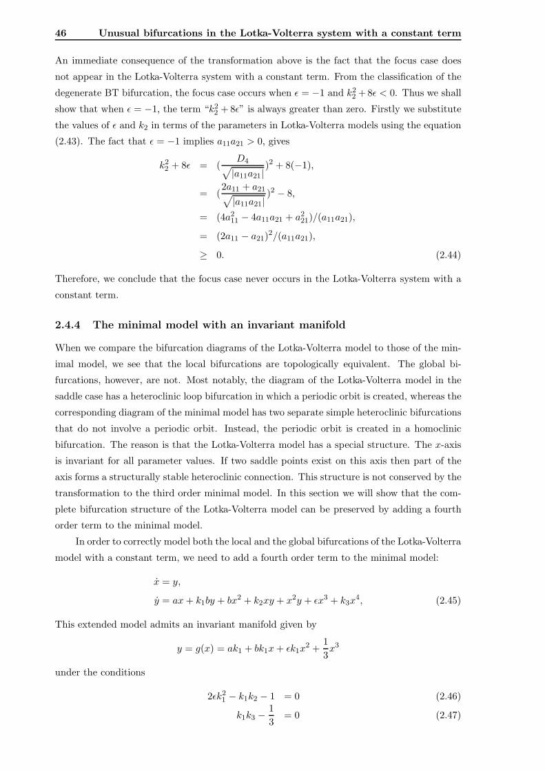
46 Unusual bifurcations in the Lotka-Volterra system with a constant term
An immediate consequence of the transformation above is the fact that the focus case does
not appear in the Lotka-Volterra system with a constant term. From the classification of the
degenerate BT bifurcation, the focus case occurs when ǫ = −1 and k22 + 8ǫ < 0. Thus we shall
show that when ǫ = −1, the term “k22 + 8ǫ” is always greater than zero. Firstly we substitute
the values of ǫ and k2 in terms of the parameters in Lotka-Volterra models using the equation
(2.43). The fact that ǫ = −1 implies a11a21 > 0, gives
k22 + 8ǫ = (
D4√
|a11a21|)2 + 8(−1),
= (2a11 + a21√
|a11a21|)2 − 8,
= (4a211 − 4a11a21 + a2
21)/(a11a21),
= (2a11 − a21)2/(a11a21),
≥ 0. (2.44)
Therefore, we conclude that the focus case never occurs in the Lotka-Volterra system with a
constant term.
2.4.4 The minimal model with an invariant manifold
When we compare the bifurcation diagrams of the Lotka-Volterra model to those of the min-
imal model, we see that the local bifurcations are topologically equivalent. The global bi-
furcations, however, are not. Most notably, the diagram of the Lotka-Volterra model in the
saddle case has a heteroclinic loop bifurcation in which a periodic orbit is created, whereas the
corresponding diagram of the minimal model has two separate simple heteroclinic bifurcations
that do not involve a periodic orbit. Instead, the periodic orbit is created in a homoclinic
bifurcation. The reason is that the Lotka-Volterra model has a special structure. The x-axis
is invariant for all parameter values. If two saddle points exist on this axis then part of the
axis forms a structurally stable heteroclinic connection. This structure is not conserved by the
transformation to the third order minimal model. In this section we will show that the com-
plete bifurcation structure of the Lotka-Volterra model can be preserved by adding a fourth
order term to the minimal model.
In order to correctly model both the local and the global bifurcations of the Lotka-Volterra
model with a constant term, we need to add a fourth order term to the minimal model:
x = y,
y = ax+ k1by + bx2 + k2xy + x2y + ǫx3 + k3x4, (2.45)
This extended model admits an invariant manifold given by
y = g(x) = ak1 + bk1x+ ǫk1x2 +
1
3x3
under the conditions
2ǫk21 − k1k2 − 1 = 0 (2.46)
k1k3 −1
3= 0 (2.47)
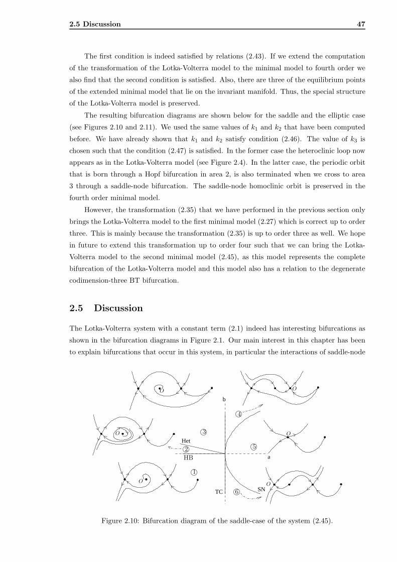
2.5 Discussion 47
The first condition is indeed satisfied by relations (2.43). If we extend the computation
of the transformation of the Lotka-Volterra model to the minimal model to fourth order we
also find that the second condition is satisfied. Also, there are three of the equilibrium points
of the extended minimal model that lie on the invariant manifold. Thus, the special structure
of the Lotka-Volterra model is preserved.
The resulting bifurcation diagrams are shown below for the saddle and the elliptic case
(see Figures 2.10 and 2.11). We used the same values of k1 and k2 that have been computed
before. We have already shown that k1 and k2 satisfy condition (2.46). The value of k3 is
chosen such that the condition (2.47) is satisfied. In the former case the heteroclinic loop now
appears as in the Lotka-Volterra model (see Figure 2.4). In the latter case, the periodic orbit
that is born through a Hopf bifurcation in area 2, is also terminated when we cross to area
3 through a saddle-node bifurcation. The saddle-node homoclinic orbit is preserved in the
fourth order minimal model.
However, the transformation (2.35) that we have performed in the previous section only
brings the Lotka-Volterra model to the first minimal model (2.27) which is correct up to order
three. This is mainly because the transformation (2.35) is up to order three as well. We hope
in future to extend this transformation up to order four such that we can bring the Lotka-
Volterra model to the second minimal model (2.45), as this model represents the complete
bifurcation of the Lotka-Volterra model and this model also has a relation to the degenerate
codimension-three BT bifurcation.
2.5 Discussion
The Lotka-Volterra system with a constant term (2.1) indeed has interesting bifurcations as
shown in the bifurcation diagrams in Figure 2.1. Our main interest in this chapter has been
to explain bifurcations that occur in this system, in particular the interactions of saddle-node
TC
a
b
SN
HetO
OO
O
OO
1
4
5
6
3
2
HB
Figure 2.10: Bifurcation diagram of the saddle-case of the system (2.45).
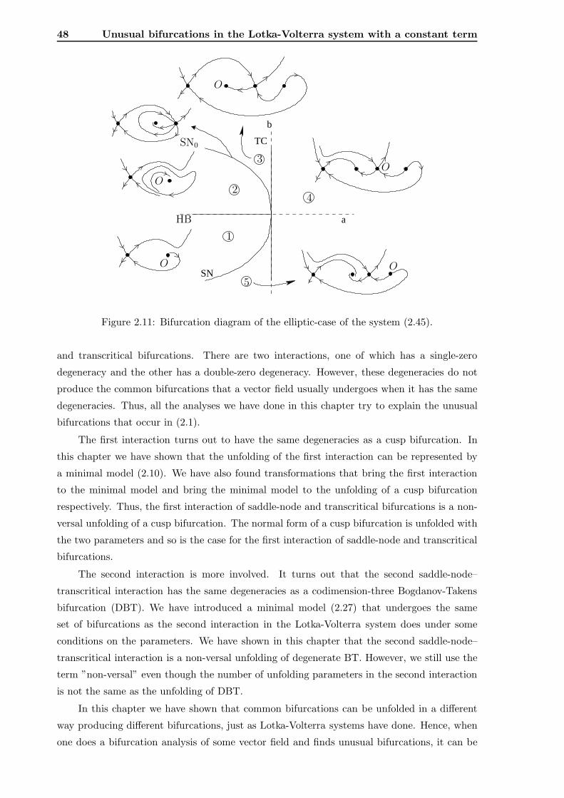
48 Unusual bifurcations in the Lotka-Volterra system with a constant term
a
b
TC
SN
2
3
1
4
O
HB
O
O
O
5
O
SN0
Figure 2.11: Bifurcation diagram of the elliptic-case of the system (2.45).
and transcritical bifurcations. There are two interactions, one of which has a single-zero
degeneracy and the other has a double-zero degeneracy. However, these degeneracies do not
produce the common bifurcations that a vector field usually undergoes when it has the same
degeneracies. Thus, all the analyses we have done in this chapter try to explain the unusual
bifurcations that occur in (2.1).
The first interaction turns out to have the same degeneracies as a cusp bifurcation. In
this chapter we have shown that the unfolding of the first interaction can be represented by
a minimal model (2.10). We have also found transformations that bring the first interaction
to the minimal model and bring the minimal model to the unfolding of a cusp bifurcation
respectively. Thus, the first interaction of saddle-node and transcritical bifurcations is a non-
versal unfolding of a cusp bifurcation. The normal form of a cusp bifurcation is unfolded with
the two parameters and so is the case for the first interaction of saddle-node and transcritical
bifurcations.
The second interaction is more involved. It turns out that the second saddle-node–
transcritical interaction has the same degeneracies as a codimension-three Bogdanov-Takens
bifurcation (DBT). We have introduced a minimal model (2.27) that undergoes the same
set of bifurcations as the second interaction in the Lotka-Volterra system does under some
conditions on the parameters. We have shown in this chapter that the second saddle-node–
transcritical interaction is a non-versal unfolding of degenerate BT. However, we still use the
term ”non-versal” even though the number of unfolding parameters in the second interaction
is not the same as the unfolding of DBT.
In this chapter we have shown that common bifurcations can be unfolded in a different
way producing different bifurcations, just as Lotka-Volterra systems have done. Hence, when
one does a bifurcation analysis of some vector field and finds unusual bifurcations, it can be
2.5 Discussion 49
explained by using the same method that we have just used in this chapter. One can explain
that the unfolding of the vector field studied is non-versal such that it has a set of unusual
bifurcations. However, this analysis triggers another question which is: why we have such
bifurcations in the first place. It turns out that when we have such unusual bifurcations, the
system must possess a special structure. The Lotka-Volterra system that has undergone such
unusual bifurcations must also have a special structure. This topic will be discussed in the
next chapter.

CHAPTER 3
Bifurcation analysis of systemshaving a codimension-one invariant
manifold
3.1 Introduction
As noticed in Wiggins [126, chapter 13], a special structure in a dynamical system greatly
constrains the type of dynamics that are allowed, and it also provides techniques of analysis
that are particular to dynamical systems with the special structure. These particular special
structures are also important because they arise in a variety of applications. One important
example of a dynamical system possessing a special structure is the Hamiltonian vector field.
Over the past years there has been a great deal of research on Hamiltonian systems. Most
research has occurred along two directions. One direction is concerned with the geometri-
cal structure of Hamilton’s equations. The other direction is concerned with the dynamical
properties of the flow generated by Hamiltonian vector fields. An excellent book on classical
mechanics, for example Abraham and Marsden [1], will outline the background for both view
points. Another example of a system with a special structure is a vector field possessing a
symmetry. This is also a broad research area in dynamical systems theory. Symmetry plays an
essential role in studying the theory and applications of dynamical systems, in particular the
influence of symmetry on normal forms, bifurcation diagrams, amongst others, see Vander-
bauwhede [121]. The symmetry property can also be used to help reduce problems in another
system with a special structure as we can see in Tuwankotta and Verhulst [119]. One type of
symmetry that often arises in applications is the reversing symmetry (see Roberts and Quis-
pel [105] and Lamb [82]). The reversing symmetry is also studied in bifurcation theories [84],
and in physics [83]. In this chapter we consider one type of dynamical system which is an
ordinary differential equation having a special structure, namely a codimension-one invariant
manifold.
52 Bifurcation analysis of systems having a codimension-one invariant manifold
3.1.1 Setting up the problem
Let us first define our problem. Suppose that we have smooth dynamical systems and we
would like to perform some (mainly bifurcation theory) analysis of the dynamics. Consider
an n-dimensional vector field, x = f(x), where x ∈ Rn and f ∈ Ck(Rn) for some k, having a
codimension-one invariant manifold. A codimension-one invariant manifold is an invariant sub-
manifold M of dimension n−1 inside an n-dimensional manifold. We are interested in a local
bifurcation analysis, say near an equilibrium. Let us assume that the equilibrium is the origin
0. Without loss of generality, near 0, the ambient manifold is Rn and the invariant manifold is
Rn−1, given in coordinates of the original manifold by saying M = {(x1, x2, . . . , xn−1, y)|y = 0}
if (x1, x2, . . . , xn−1, y) are the Rn coordinates. And we assume that any smooth codimension-
one manifold can be rectified this way.
Example 3.4 (One-dimensional case). Suppose we have a one-dimensional dynamical system
having a codimension-one invariant manifold. The origin, 0 will be our invariant manifold.
Locally, we can define our dynamical system as follows,
y = yf(y) y ∈ R, (3.1)
where f(y) is some function in R.
Example 3.5 (n-dimensional case). Suppose that we have an n-dimensional vector field,
x = f(x) ∈ Rn having a codimension-one invariant manifold, then the vector field can be
written as follows,
x1 = f1(x1, x2, . . . , xn−1, y),
x2 = f2(x1, x2, . . . , xn−1, y),...
xn−1 = fn−1(x1, x2, . . . , xn−1, y),
y = yfn(x1, x2, . . . , xn−1, y).
(3.2)
The invariant manifold M is invariant with respect to the above differential equation, (i.e.
M is said to be invariant under the vector field ξ = φ(ξ) if for any ξ0 ∈ M ⊂ Rn we have
ξ(t, ξ0) ∈M for all t ∈ R).
Let us look at the n× n Jacobian matrix of the system (3.2), evaluated at the origin 0,
J(0) =
∂f1
∂x1(0) ∂f1
∂x2. . . ∂f1
∂xn−1(0) ∂f1
∂y(0)
∂f2
∂x1(0) ∂f2
∂x2. . . ∂f2
∂xn−1(0) ∂f2
∂y(0)
.... . .
...∂fn−1
∂x1(0) ∂fn−1
∂x2. . . ∂fn−1
∂xn−1(0) ∂fn−1
∂y(0)
0 0 . . . 0 fn(0)
(3.3)
The eigenvalues of the above matrix are fn(0) and all eigenvalues of the (n − 1) × (n − 1)
matrix below,
∂f1
∂x1(0) ∂f1
∂x2. . . ∂f1
∂xn−1(0)
∂f2
∂x1(0) ∂f2
∂x2. . . ∂f2
∂xn−1(0)
......
∂fn−1
∂x1(0) ∂fn−1
∂x2. . . ∂fn−1
∂xn−1(0)
. (3.4)
3.1 Introduction 53
The simplest degeneracies are a single-zero eigenvalue and a pair of purely imaginary eigenvalue
degeneracies. We have our first proposition.
Proposition 3.6. The center manifold of an equilibrium having a single-zero eigenvalue or
a pair of purely imaginary eigenvalue of the matrix (3.4) lies inside the codimension-one
invariant manifold up to any desired degree of accuracy.
Proof. See Appendix A.
Our general purpose is to describe all the low codimension bifurcations of equilibria and
perhaps periodic orbits in such a way that the property of having an invariant manifold M is
always preserved and the manifold remains the same. Our bifurcation analysis of dynamical
systems with a special structure will be analogous to that of general dynamical systems in
which we do not have a special structure. First we want to classify possible low codimension
bifurcations. Note that we only discuss codimension-one and codimension-two bifurcations.
Codimension-one bifurcations have two types of degeneracy, namely a single zero eigenvalue
and a pair of purely imaginary eigenvalues. In general systems, these conditions yield saddle-
node and Hopf bifurcations respectively. However, when the system has a codimension-one
invariant manifold we may not have such bifurcations.
We will not discuss the cases where the center manifold lies entirely in the invariant
manifold M since they correspond to the usual generic bifurcations. Since the complex pair
of eigenvalues can only come from the matrix (3.4) the center manifold of the pair of purely
imaginary eigenvalues degeneracy lies inside the invariant manifold M . Thus, we shall not
analyse the Hopf bifurcation because it will be similar to the generic case. If the single-zero
eigenvalue comes from the matrix (3.4) it will also not be of interest for the same reason.
Hence the only degeneracy for a codimension-one bifurcation that we are going to discuss is
a single-zero eigenvalue degeneracy where fn(0) = 0.
Codimension-two bifurcations give us more possibilities. We start with the same degener-
acy as the codimension-one bifurcations have, but now we will have an additional degeneracy
in the nonlinear terms of the normal form. We shall get bifurcations whose codimension are
higher by studying a degeneracy that comes from higher order terms or non-linear terms of
the function fn(x1, x2, . . . , y). We then also consider cases in which the linear part of the
vector field is doubly degenerate. The eigenvalues of the matrix (3.4) are now allowed to have
degeneracies, whether they are zero or purely imaginary. Combined with the first single-zero
degeneracy, the center manifold will not lie entirely inside the invariant manifold. These ad-
ditional degeneracies also allow the system to have codimension-two (or higher) bifurcations.
Firstly we shall discuss the double zero eigenvalue degeneracy. In a general system, this cor-
responds to the Bogdanov-Takens bifurcation. Secondly we have a single zero eigenvalue with
a pair of purely imaginary eigenvalues that corresponds to a saddle-Hopf bifurcation in the
general system.
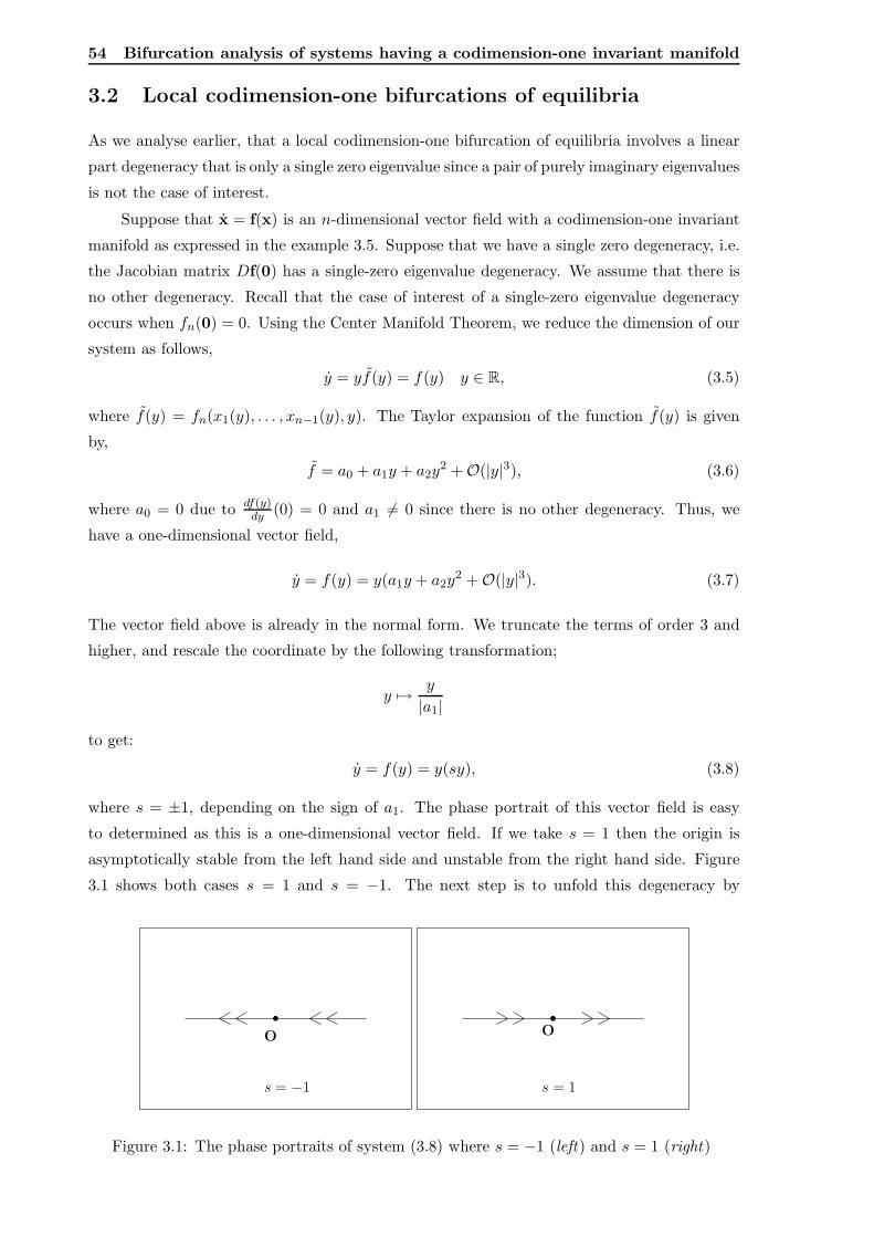
54 Bifurcation analysis of systems having a codimension-one invariant manifold
3.2 Local codimension-one bifurcations of equilibria
As we analyse earlier, that a local codimension-one bifurcation of equilibria involves a linear
part degeneracy that is only a single zero eigenvalue since a pair of purely imaginary eigenvalues
is not the case of interest.
Suppose that x = f(x) is an n-dimensional vector field with a codimension-one invariant
manifold as expressed in the example 3.5. Suppose that we have a single zero degeneracy, i.e.
the Jacobian matrix Df(0) has a single-zero eigenvalue degeneracy. We assume that there is
no other degeneracy. Recall that the case of interest of a single-zero eigenvalue degeneracy
occurs when fn(0) = 0. Using the Center Manifold Theorem, we reduce the dimension of our
system as follows,
y = yf(y) = f(y) y ∈ R, (3.5)
where f(y) = fn(x1(y), . . . , xn−1(y), y). The Taylor expansion of the function f(y) is given
by,
f = a0 + a1y + a2y2 + O(|y|3), (3.6)
where a0 = 0 due to df(y)dy
(0) = 0 and a1 6= 0 since there is no other degeneracy. Thus, we
have a one-dimensional vector field,
y = f(y) = y(a1y + a2y2 + O(|y|3). (3.7)
The vector field above is already in the normal form. We truncate the terms of order 3 and
higher, and rescale the coordinate by the following transformation;
y 7→ y
|a1|
to get:
y = f(y) = y(sy), (3.8)
where s = ±1, depending on the sign of a1. The phase portrait of this vector field is easy
to determined as this is a one-dimensional vector field. If we take s = 1 then the origin is
asymptotically stable from the left hand side and unstable from the right hand side. Figure
3.1 shows both cases s = 1 and s = −1. The next step is to unfold this degeneracy by
O O
s = −1 s = 1
Figure 3.1: The phase portraits of system (3.8) where s = −1 (left) and s = 1 (right)
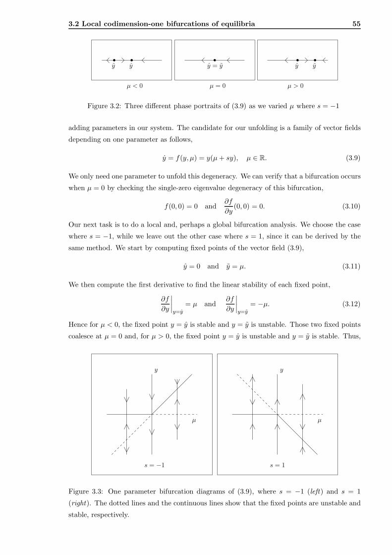
3.2 Local codimension-one bifurcations of equilibria 55
y = y y yy y
µ < 0 µ = 0 µ > 0
Figure 3.2: Three different phase portraits of (3.9) as we varied µ where s = −1
adding parameters in our system. The candidate for our unfolding is a family of vector fields
depending on one parameter as follows,
y = f(y, µ) = y(µ+ sy), µ ∈ R. (3.9)
We only need one parameter to unfold this degeneracy. We can verify that a bifurcation occurs
when µ = 0 by checking the single-zero eigenvalue degeneracy of this bifurcation,
f(0, 0) = 0 and∂f
∂y(0, 0) = 0. (3.10)
Our next task is to do a local and, perhaps a global bifurcation analysis. We choose the case
where s = −1, while we leave out the other case where s = 1, since it can be derived by the
same method. We start by computing fixed points of the vector field (3.9),
y = 0 and y = µ. (3.11)
We then compute the first derivative to find the linear stability of each fixed point,
∂f
∂y
∣
∣
∣
∣
y=y
= µ and∂f
∂y
∣
∣
∣
∣
y=y
= −µ. (3.12)
Hence for µ < 0, the fixed point y = y is stable and y = y is unstable. Those two fixed points
coalesce at µ = 0 and, for µ > 0, the fixed point y = y is unstable and y = y is stable. Thus,
y
µ
s = −1 s = 1
µ
y
Figure 3.3: One parameter bifurcation diagrams of (3.9), where s = −1 (left) and s = 1
(right). The dotted lines and the continuous lines show that the fixed points are unstable and
stable, respectively.
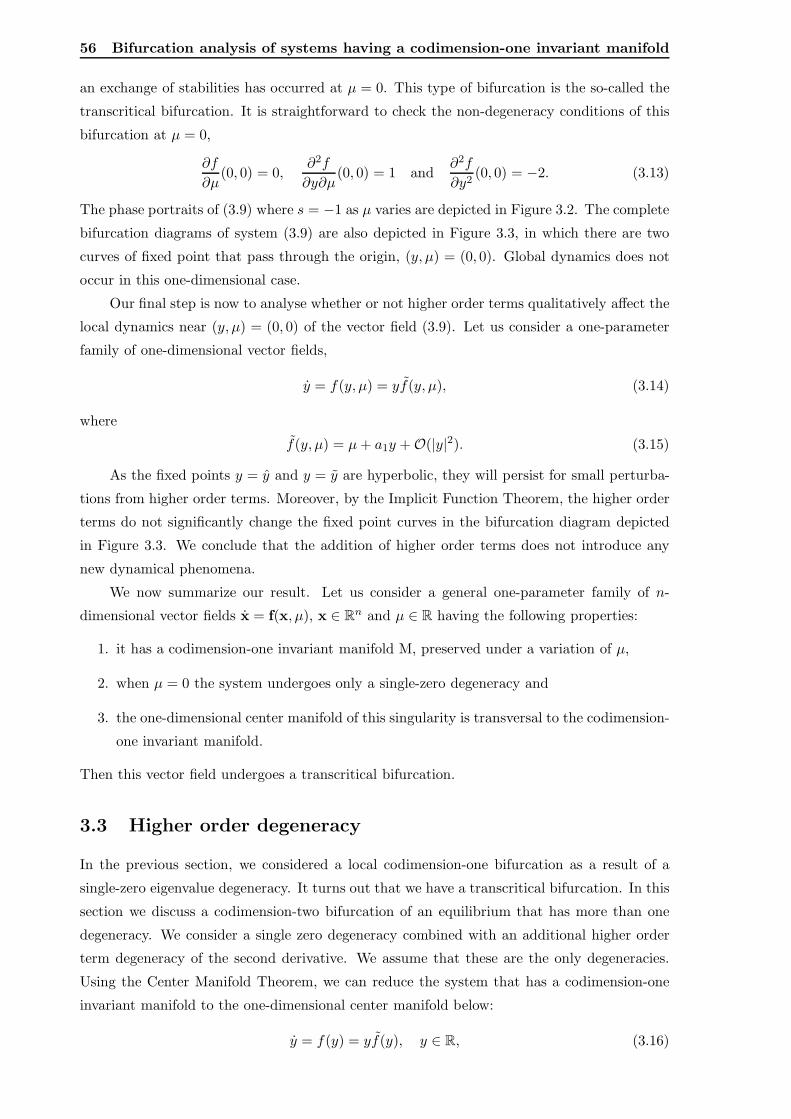
56 Bifurcation analysis of systems having a codimension-one invariant manifold
an exchange of stabilities has occurred at µ = 0. This type of bifurcation is the so-called the
transcritical bifurcation. It is straightforward to check the non-degeneracy conditions of this
bifurcation at µ = 0,
∂f
∂µ(0, 0) = 0,
∂2f
∂y∂µ(0, 0) = 1 and
∂2f
∂y2(0, 0) = −2. (3.13)
The phase portraits of (3.9) where s = −1 as µ varies are depicted in Figure 3.2. The complete
bifurcation diagrams of system (3.9) are also depicted in Figure 3.3, in which there are two
curves of fixed point that pass through the origin, (y, µ) = (0, 0). Global dynamics does not
occur in this one-dimensional case.
Our final step is now to analyse whether or not higher order terms qualitatively affect the
local dynamics near (y, µ) = (0, 0) of the vector field (3.9). Let us consider a one-parameter
family of one-dimensional vector fields,
y = f(y, µ) = yf(y, µ), (3.14)
where
f(y, µ) = µ+ a1y + O(|y|2). (3.15)
As the fixed points y = y and y = y are hyperbolic, they will persist for small perturba-
tions from higher order terms. Moreover, by the Implicit Function Theorem, the higher order
terms do not significantly change the fixed point curves in the bifurcation diagram depicted
in Figure 3.3. We conclude that the addition of higher order terms does not introduce any
new dynamical phenomena.
We now summarize our result. Let us consider a general one-parameter family of n-
dimensional vector fields x = f(x, µ), x ∈ Rn and µ ∈ R having the following properties:
1. it has a codimension-one invariant manifold M, preserved under a variation of µ,
2. when µ = 0 the system undergoes only a single-zero degeneracy and
3. the one-dimensional center manifold of this singularity is transversal to the codimension-
one invariant manifold.
Then this vector field undergoes a transcritical bifurcation.
3.3 Higher order degeneracy
In the previous section, we considered a local codimension-one bifurcation as a result of a
single-zero eigenvalue degeneracy. It turns out that we have a transcritical bifurcation. In this
section we discuss a codimension-two bifurcation of an equilibrium that has more than one
degeneracy. We consider a single zero degeneracy combined with an additional higher order
term degeneracy of the second derivative. We assume that these are the only degeneracies.
Using the Center Manifold Theorem, we can reduce the system that has a codimension-one
invariant manifold to the one-dimensional center manifold below:
y = f(y) = yf(y), y ∈ R, (3.16)
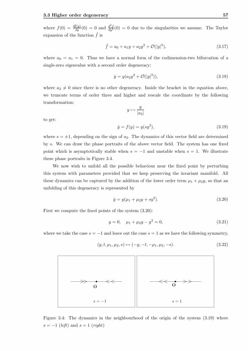
3.3 Higher order degeneracy 57
where f(0) = df(y)dy
(0) = 0 and d2fdy2 (0) = 0 due to the singularities we assume. The Taylor
expansion of the function f is
f = a0 + a1y + a2y2 + O(|y|3), (3.17)
where a0 = a1 = 0. Thus we have a normal form of the codimension-two bifurcation of a
single-zero eigenvalue with a second order degeneracy:
y = y(a2y2 + O(|y|3)), (3.18)
where a2 6= 0 since there is no other degeneracy. Inside the bracket in the equation above,
we truncate terms of order three and higher and rescale the coordinate by the following
transformation:
y 7→ y
|a2|to get:
y = f(y) = y(sy2), (3.19)
where s = ±1, depending on the sign of a2. The dynamics of this vector field are determined
by s. We can draw the phase portraits of the above vector field. The system has one fixed
point which is asymptotically stable when s = −1 and unstable when s = 1. We illustrate
these phase portraits in Figure 3.4.
We now wish to unfold all the possible behaviour near the fixed point by perturbing
this system with parameters provided that we keep preserving the invariant manifold. All
these dynamics can be captured by the addition of the lower order term µ1 + µ2y, so that an
unfolding of this degeneracy is represented by
y = y(µ1 + µ2y + sy2). (3.20)
First we compute the fixed points of the system (3.20):
y = 0, µ1 + µ2y − y2 = 0, (3.21)
where we take the case s = −1 and leave out the case s = 1 as we have the following symmetry,
(y, t, µ1, µ2, s) 7→ (−y,−t,−µ1, µ2,−s). (3.22)
O O
s = −1 s = 1
Figure 3.4: The dynamics in the neighbourhood of the origin of the system (3.19) where
s = −1 (left) and s = 1 (right)
58 Bifurcation analysis of systems having a codimension-one invariant manifold
Hence we always have y0 = 0 as our fixed point while the other fixed points can be found by
computing:
y1,2 =µ2 ±
√
µ 22 + 4µ1
2. (3.23)
From the local analysis above, we conclude that when the term µ 22 + 4µ1 is positive there
are three fixed points and when µ 22 + 4µ1 is negative we have the origin as the only fixed
point. Furthermore, when the term µ 22 + 4µ1 is zero, the fixed points y1 and y2 collide into
one equilibrium in a saddle-node bifurcation. We set f(y, µ1) = y(µ1 + µ2y − y2). We now
check conditions of this bifurcation at µ1 = −µ 22 /4,
∂f
∂y(y1,−
µ 22
4) =
∂f
∂y(y2,−
µ 22
4) = 0,
∂f
∂µ1(y1,−
µ 22
4) =
∂f
∂µ1(y2,−
µ 22
4) =
µ2
2
and∂2f
∂y2(y1,−
µ 22
4) =
∂2f
∂y2(y2,−
µ 22
4) = −µ2. (3.24)
Hence, we conclude that a non-degenerate saddle-node bifurcation occurs along the curve
µ 22 + 4µ1 = 0 but µ2 6= 0.
When µ1 = 0 and µ2 < 0 (µ2 > 0 respectively), the equilibrium y1 (y2 respectively)
coincides with y0. The stabilities of these fixed points are determined by:
∂f
∂y(y, µ1) = µ1 + 2µ2y − 3y2. (3.25)
Then we compute the eigenvalues of both equilibria,
∂f
∂y(y0, µ1) = µ1 and
∂f
∂y(y1,2, µ1) =
1
2(µ2 ±
√
µ 22 + 4µ1)
√
µ 22 + 4µ1. (3.26)
We consider case when µ2 > 0. When µ1 > 0 the equilibrium y = y0 is unstable as its
eigenvalue is positive and the equilibrium y = y2 is stable as its eigenvalue is negative. On the
other hand, when µ1 < 0 the equilibria y = 0 and y = y1 are stable and unstable respectively.
Hence, an exchange of stabilities occurs as they coincide when µ1 = 0 in a transcritical
bifurcation. We check the non-degeneracy conditions of this bifurcation,
∂f
∂µ1(0, 0) = 0,
∂2f
∂y∂µ1(0, 0) = 1 and
∂2f
∂y2(0, 0) = 2µ2, (3.27)
to conclude that a non-degenerate transcritical bifurcation occurs along the curve µ1 = 0 but
µ2 6= 0.
Thus, we shall have two bifurcation curves in our parameter space, which are the saddle-
node and transcritical bifurcations. Both bifurcation curves coincide when µ1 = µ2 = 0 at
which the degeneracy of a single-zero eigenvalue with a second order degeneracy occurs. All
these dynamics are illustrated in Figure 3.5. We have an interaction of the saddle-node and
the transcritical bifurcations at (µ1, µ2) = (0, 0).
We now analyse the effect of higher order terms. First we put them back in (3.20),
y = y(µ1 + µ2y − y2 + O(|y|3)), (3.28)
where y, µ1, µ2 ∈ R. The addition of higher order terms does not affect the existence and
the stability of the fixed points (y = y0, y = y1 and y = y2) because of the fact that
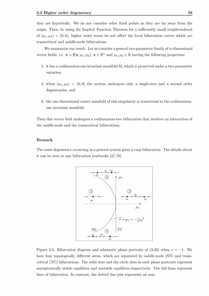
3.3 Higher order degeneracy 59
they are hyperbolic. We do not consider other fixed points as they are far away from the
origin. Then, by using the Implicit Function Theorem for a sufficiently small neighbourhood
of (µ1, µ2) = (0, 0), higher order terms do not affect the local bifurcation curves which are
transcritical and saddle-node bifurcations.
We summarize our result. Let us consider a general two-parameter family of n-dimensional
vector fields, i.e. x = f(x, µ1, µ2), x ∈ Rn and µ1, µ2 ∈ R having the following properties:
1. it has a codimension-one invariant manifold M, which is preserved under a two-parameter
variation.
2. when (µ1, µ2) = (0, 0) the system undergoes only a single-zero and a second order
degeneracies, and
3. the one-dimensional center manifold of this singularity is transversal to the codimension-
one invariant manifold.
Then this vector field undergoes a codimension-two bifurcation that involves an interaction of
the saddle-node and the transcritical bifurcations.
Remark
The same degeneracy occurring in a general system gives a cusp bifurcation. The details about
it can be seen in any bifurcation textbooks [47,78].
µ1
y0
µ2
SN TCy2
y0
y1
y0
y2y1
1
2
4
3
y0
y2y1
µ1 = −14µ
22
Figure 3.5: Bifurcation diagram and schematic phase portraits of (3.20) when s = −1. We
have four topologically different areas, which are separated by saddle-node (SN) and trans-
critical (TC) bifurcations. The solid dots and the circle dots in each phase portraits represent
asymptotically stable equilibria and unstable equilibria respectively. The full lines represent
lines of bifurcation. In contrast, the dotted line just represents an axis.
60 Bifurcation analysis of systems having a codimension-one invariant manifold
3.4 Double zero eigenvalue degeneracy
3.4.1 Normal form derivation
Consider the equation (3.2). We know that a codimension-one bifurcation (i.e. the transcritical
bifurcation) occurs when
fn(0) = 0.
The other degeneracy possibly comes from the matrix (3.4). This is the case in this section,
where in particular we consider a double-zero eigenvalue degeneracy. The Jordan canonical
form of the linear part of the system with a double-zero eigenvalue degeneracy is given by,
A =
(
0 1
0 0
)
. (3.29)
We work on a two-dimensional system since the center manifold of this degeneracy is two-
dimensional, thus we have a system of two differential equations,
x = y + O(‖(x, y)‖2),
y = y(O(‖(x, y)‖1),(3.30)
where O(‖(x, y)‖k) is defined below,
O(‖(x, y)‖k) =
k∑
i=0
β(k−i)ixk−iyi + O(‖(x, y)‖k+1),
where k is an integer greater than zero. We shall do a normalization to find a coordinate
system in which our dynamical system is as simple as possible. To start the normalization
treatment of a system having a codimension-one invariant manifold, we consider the range of
the operator ad A = [., A] that is spanned by these four vectors:
{(
2xy
0
)
,
(
−y2
0
)
,
(
xy
−y2
)
,
(
y2
0
)}
. (3.31)
These vectors are, respectively, the Lie brackets of the linear part of (3.30) with the five
standard basis vectors for H2(R2), which is the space of the polynomial vector fields of degree
2, having a codimension-one invariant manifold, (note that the Lie bracket with the third term
below is identically zero),
{(
x2
0
)
,
(
xy
0
)
,
(
y2
0
)
,
(
0
xy
)
,
(
0
y2
)}
. (3.32)
Thus, the set of vectors below,{(
x2
0
)
,
(
0
xy
)
,
}
(3.33)
spans a complementary subspace of the range of the operator ad A. Hence, the normal form
of (3.30) can be written as:
x = y + ax2 + O(||(x, y)||3),
y = y(bx+ O(||(x, y)||2)).(3.34)
3.4 Double zero eigenvalue degeneracy 61
We assume that there is no other degeneracy, which means that the quadratic coefficients of
the normal form above, a and b do not vanish. We initially neglect terms of order three and
higher to have a two-dimensional normal form:
x = y + ax2,
y = y(bx).(3.35)
3.4.2 Phase portrait of normal forms with a double zero degeneracy
We would like to sketch the dynamics of the system (3.35) near the origin. Using the following
transformation:
x 7→ v = x, y 7→ w = y + ax2, (3.36)
we get a new system,
v = w,
w = (2a+ b)vw − abv3,(3.37)
which is a codimension-three Bogdanov-Takens degeneracy (see Dumortier et al. [31]). The
normal form of the codimension-three Bogdanov-Takens bifurcation is given by
ξ1 = ξ2,
ξ2 = Bξ1ξ2 + ǫ1ξ31 +Dξ21ξ2 + Eξ41 + O(||ξ1, ξ2||5)
(3.38)
where Bǫ1 6= 0. The topological dynamics near the origin of the system above (3.38) are
distinguished [31] as follows:
• saddle case ǫ1 > 0, any B and D;
• focus case ǫ1 < 0 and B2 + 8ǫ1 < 0;
• elliptic case ǫ1 < 0 and B2 + 8ǫ1 > 0.
The bifurcation is defined to be regular if the parameters satisfy another extra condition below,
5ǫ1D − 3BE 6= 0. (3.39)
Applying the information above to the equation (3.37) we perform a simple calculation to get
a classification for (3.35),
• saddle case ab < 0,
• elliptic case ab > 0,
where 2a + b 6= 0 since the codimension-three Bogdanov-Takens bifurcation does not allow
the coefficients of ”vw” and ”v3” in the normal form (3.37) to be zero. One may notice
that our bifurcation seems more degenerate due to a violation of the condition (3.39). It is
mainly because we truncate the higher order terms of the normal form (3.34) that affects the
topological dynamics of our vector field. We shall discuss this later on in this section.
However in our classification, we do not have the focus case. This fact is expected as
we have an invariant manifold near the origin. The schematic phase portraits can be seen in
Figure 3.6.
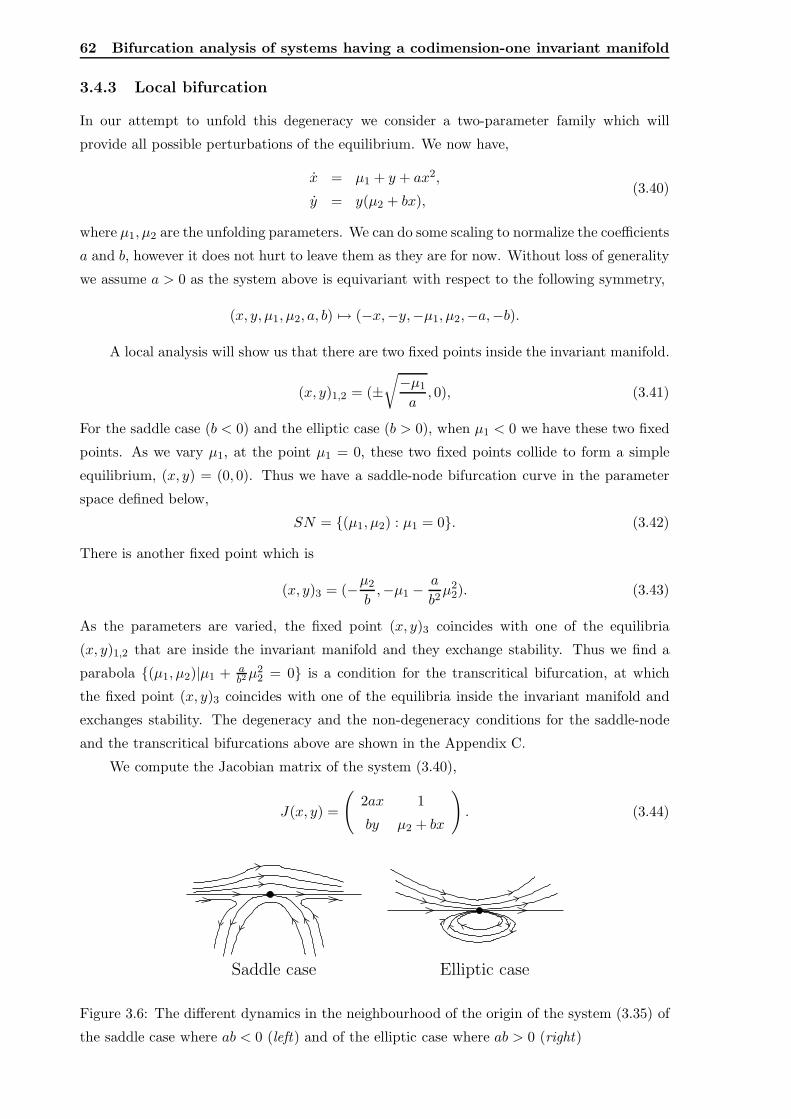
62 Bifurcation analysis of systems having a codimension-one invariant manifold
3.4.3 Local bifurcation
In our attempt to unfold this degeneracy we consider a two-parameter family which will
provide all possible perturbations of the equilibrium. We now have,
x = µ1 + y + ax2,
y = y(µ2 + bx),(3.40)
where µ1, µ2 are the unfolding parameters. We can do some scaling to normalize the coefficients
a and b, however it does not hurt to leave them as they are for now. Without loss of generality
we assume a > 0 as the system above is equivariant with respect to the following symmetry,
(x, y, µ1, µ2, a, b) 7→ (−x,−y,−µ1, µ2,−a,−b).
A local analysis will show us that there are two fixed points inside the invariant manifold.
(x, y)1,2 = (±√
−µ1
a, 0), (3.41)
For the saddle case (b < 0) and the elliptic case (b > 0), when µ1 < 0 we have these two fixed
points. As we vary µ1, at the point µ1 = 0, these two fixed points collide to form a simple
equilibrium, (x, y) = (0, 0). Thus we have a saddle-node bifurcation curve in the parameter
space defined below,
SN = {(µ1, µ2) : µ1 = 0}. (3.42)
There is another fixed point which is
(x, y)3 = (−µ2
b,−µ1 −
a
b2µ2
2). (3.43)
As the parameters are varied, the fixed point (x, y)3 coincides with one of the equilibria
(x, y)1,2 that are inside the invariant manifold and they exchange stability. Thus we find a
parabola {(µ1, µ2)|µ1 + ab2µ2
2 = 0} is a condition for the transcritical bifurcation, at which
the fixed point (x, y)3 coincides with one of the equilibria inside the invariant manifold and
exchanges stability. The degeneracy and the non-degeneracy conditions for the saddle-node
and the transcritical bifurcations above are shown in the Appendix C.
We compute the Jacobian matrix of the system (3.40),
J(x, y) =
(
2ax 1
by µ2 + bx
)
. (3.44)
Saddle case Elliptic case
Figure 3.6: The different dynamics in the neighbourhood of the origin of the system (3.35) of
the saddle case where ab < 0 (left) and of the elliptic case where ab > 0 (right)
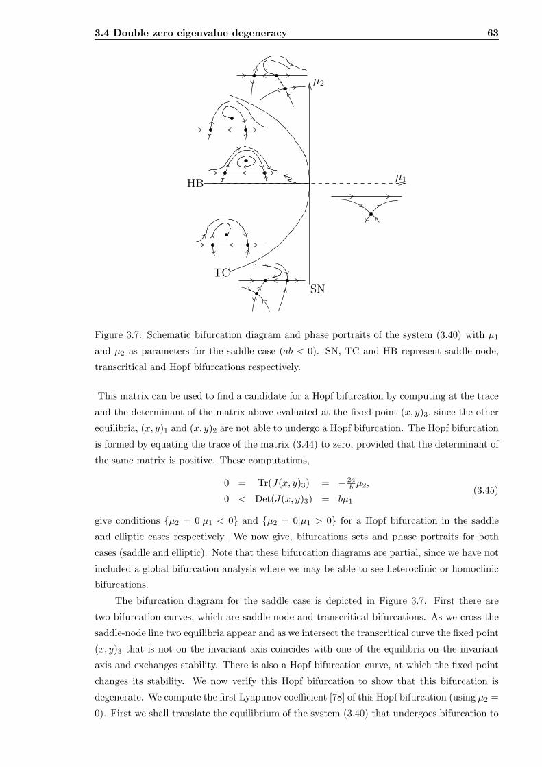
3.4 Double zero eigenvalue degeneracy 63
HB
TC
SN
µ2
µ1
Figure 3.7: Schematic bifurcation diagram and phase portraits of the system (3.40) with µ1
and µ2 as parameters for the saddle case (ab < 0). SN, TC and HB represent saddle-node,
transcritical and Hopf bifurcations respectively.
This matrix can be used to find a candidate for a Hopf bifurcation by computing at the trace
and the determinant of the matrix above evaluated at the fixed point (x, y)3, since the other
equilibria, (x, y)1 and (x, y)2 are not able to undergo a Hopf bifurcation. The Hopf bifurcation
is formed by equating the trace of the matrix (3.44) to zero, provided that the determinant of
the same matrix is positive. These computations,
0 = Tr(J(x, y)3) = −2abµ2,
0 < Det(J(x, y)3) = bµ1
(3.45)
give conditions {µ2 = 0|µ1 < 0} and {µ2 = 0|µ1 > 0} for a Hopf bifurcation in the saddle
and elliptic cases respectively. We now give, bifurcations sets and phase portraits for both
cases (saddle and elliptic). Note that these bifurcation diagrams are partial, since we have not
included a global bifurcation analysis where we may be able to see heteroclinic or homoclinic
bifurcations.
The bifurcation diagram for the saddle case is depicted in Figure 3.7. First there are
two bifurcation curves, which are saddle-node and transcritical bifurcations. As we cross the
saddle-node line two equilibria appear and as we intersect the transcritical curve the fixed point
(x, y)3 that is not on the invariant axis coincides with one of the equilibria on the invariant
axis and exchanges stability. There is also a Hopf bifurcation curve, at which the fixed point
changes its stability. We now verify this Hopf bifurcation to show that this bifurcation is
degenerate. We compute the first Lyapunov coefficient [78] of this Hopf bifurcation (using µ2 =
0). First we shall translate the equilibrium of the system (3.40) that undergoes bifurcation to

64 Bifurcation analysis of systems having a codimension-one invariant manifold
the origin, using the following transformation:
(x, y) 7→ (x, y) = (x/√
bµ1, y + µ1),
to get a new system in the form,
˙x =√bµ1y + a√
bµ1
x2,
˙y = −√bµ1x+ b√
bµ1
xy,
where bµ1 > 0. Using the system above, we determine that the first Lyapunov coefficient of
the Hopf bifurcation above is zero. This implies that the terms of at least cubic order in our
normal form must be included. In fact, for µ2 = 0 (where the Hopf bifurcation occurs) the
system (3.40) is completely integrable, since the function
F (x, y) = −by− 2ab (µ1
2a+
y
2a− b+x2
2) (3.46)
is constant along the solution of (3.40),
F = ∂F∂xx+ ∂F
∂yy,
= (−by− 2ab x)(µ1 + y + ax2) + y−
2ab (µ1
y+ 1 + ax2
y)(bxy),
= 0.
(3.47)
This integral function holds if 2a − b 6= 0, however if this is not the case we still have an
integral but it will not be of this form. This implies that when the Hopf bifurcation occurs in
our system, we will have infinitely many periodic orbits and a heteroclinic link between two
saddle equilibria that are living inside the codimension-one invariant manifold. This can be
seen in the phase portrait of Figure 3.7, when µ2 = 0 and µ1 < 0.
The bifurcation diagram for the elliptic case is depicted in Figure 3.8. We still have curves
of saddle-node and transcritical bifurcations, however a Hopf bifurcation occurs at the other
side of the plane (when µ2 = 0 and µ1 > 0). The Hopf bifurcation is again degenerate since
it is undetermined by the quadratic normal form. Furthermore, the system is also completely
integrable with the same integral function (3.46) when µ2 = 0 at which the Hopf bifurcation
occurs. We still have the fact that there are infinitely many periodic orbits, but we do not have
a global bifurcation phenomenon. This permits us to conclude the local unfolding analysis of
system (3.35).
We now address the effect of higher order terms in our planar system and show that some
results we have ”survive” while others do not. Consider the vector field (3.40) with additional
higher order terms:
x = µ1 + y + ax2 + O(‖(x, y)‖3),
y = y(µ2 + bx+ O(‖(x, y)‖2)),(3.48)
By performing computations on the equations above we immediately find that the number
of fixed points of the system (3.48) is more than the number of fixed points of the system
without higher order terms (3.40) since the degree of the fixed point equations is higher.
However, we are only interested in the neighbourhood of (µ1, µ2) = (0, 0). Hence, we have
the same number of equilibria involved between the system (3.40) and (3.48) locally near
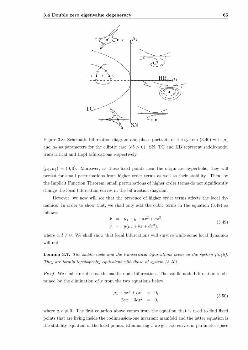
3.4 Double zero eigenvalue degeneracy 65
µ2
TC
SN
µ1HB
Figure 3.8: Schematic bifurcation diagram and phase portraits of the system (3.40) with µ1
and µ2 as parameters for the elliptic case (ab > 0). SN, TC and HB represent saddle-node,
transcritical and Hopf bifurcations respectively.
(µ1, µ2) = (0, 0). Moreover, as those fixed points near the origin are hyperbolic, they will
persist for small perturbations from higher order terms as well as their stability. Then, by
the Implicit Function Theorem, small perturbations of higher order terms do not significantly
change the local bifurcation curves in the bifurcation diagram.
However, we now will see that the presence of higher order terms affects the local dy-
namics. In order to show that, we shall only add the cubic terms in the equation (3.48) as
follows:
x = µ1 + y + ax2 + cx3,
y = y(µ2 + bx+ dx2),(3.49)
where c, d 6= 0. We shall show that local bifurcations will survive while some local dynamics
will not.
Lemma 3.7. The saddle-node and the transcritical bifurcations occur in the system (3.49).
They are locally topologically equivalent with those of system (3.40).
Proof. We shall first discuss the saddle-node bifurcation. The saddle-node bifurcation is ob-
tained by the elimination of x from the two equations below,
µ1 + ax2 + cx3 = 0,
2ax+ 3cx2 = 0,(3.50)
where a, c 6= 0. The first equation above comes from the equation that is used to find fixed
points that are living inside the codimension-one invariant manifold and the latter equation is
the stability equation of the fixed points. Eliminating x we get two curves in parameter space
66 Bifurcation analysis of systems having a codimension-one invariant manifold
that give saddle-node bifurcations,
µ1 = 0 and µ1 =4a3
27c2. (3.51)
However, we do not consider the bifurcation curve in the part of parameter space that is
outside the neighbourhood of the origin, (µ1, µ2) = (0, 0), thus we are only interested in the
first saddle-node bifurcation curve, µ1 = 0. This curve, in fact is the same curve as the
saddle-node bifurcation curve of system (3.40), thus we have proved the first part of this
lemma.
To prove the second part of this lemma, we consider these two equations,
µ1 + ax2 + cx3 = 0,
µ2 + bx+ dx2 = 0,(3.52)
where a, b, c, d 6= 0. The first equation comes from the equation, used to find the condition
for the fixed point to cross the invariant manifold, coincide and exchange stability with the
fixed point that is inside the manifold, y = 0, while the second equation comes from the
condition that the eigenvalue of the Jacobian matrix evaluated at the critical fixed point is
zero. Eliminating x from the two equations above gives us a curve of transcritical bifurcation
in the parameter space µ1 − µ2. We want to prove that this bifurcation curve is topologically
equivalent to the transcritical bifurcation curve of system (3.40). We consider the equations
above as a non-linear system of two equations with coordinates (x, µ1, µ2) as follows,
φ(x, µ1, µ2) =
{
φ1(x, µ1, µ2) = µ2 + bx+ dx2 = 0,
φ1(x, µ1, µ2) = µ1 + ax2 + cx3 = 0.(3.53)
The solution of the non-linear system above is a curve, passing through the origin since (0, 0, 0)
satisfies the equations above. The Jacobian matrix of the non-linear system above evaluated
at the origin,
J(0, 0, 0) =
(
b 0 1
0 1 0
)
,
has rank two since the determinant of the sub-matrix below is not zero,
det
(
0 1
1 0
)
6= 0.
In this case, the Implicit Function Theorem provides the local existence of two smooth func-
tions, µ1(x) and µ2(x) for x sufficiently near the origin,
µ1(x) = −ax2 − c3, and µ2(x) = −bx− dx2.
These functions in fact define a curve γ ⊂ R2 that is the transcritical bifurcation curve in the
parameter space µ1 − µ2, parameterized by an interval of x near zero. This curve, moreover
has the following characteristics: it is tangent to the saddle-node bifurcation line µ1 = 0,
dµ1
dµ2(0, 0) =
dµ1
dx(0)
dµ2
dx(0)
= 0,
3.4 Double zero eigenvalue degeneracy 67
it passes the origin (µ1, µ2) = (0, 0), and the sign of µ1-coordinate is negative for a > 0 for
sufficiently small x near zero. These characteristics are also the case for the transcritical
bifurcation of system (3.40). We now have a rough picture of this transcritical bifurcation
curve. And now we want to construct a local homeomorphism of the parameter plane that
maps this curve into the corresponding transcritical bifurcation curve of system (3.40) as
shown in Figures 3.7 and 3.8 for saddle and elliptic cases respectively. The idea is to use
the property of the parametrization of the curve γ and the fact that the transcritical curve
of (3.40) can also be parameterized by the same interval. The Implicit Function Theorem
guarantees that the parametrization of the curve γ is locally one-to-one. Using this property,
we can construct an inverse transformation to map a point in the curve γ to the interval near
x = 0. Finally, the image of this inverse parametrization is mapped to the parabolic curve of
the transcritical bifurcation of the system (3.40). Thus, we have shown that the transcritical
bifurcation curve of (3.49) is locally topologically equivalent with that of system (3.40).
Lemma 3.8. Consider system (3.49) with a > 0. A Hopf bifurcation occurs when µ2 = 0,
µ1 < 0 for the saddle case and µ2 = 0, µ1 > 0 for the elliptic case. This Hopf bifurcation is
non-degenerate.
Proof. The first equation for the Hopf bifurcation is obtained by evaluating the critical equi-
librium that is not on the invariant manifold. Thus y 6= 0 in the equation (3.49), and it implies
that µ2 + bx+ dx2 must be equal to zero. We now have to compute the trace of the Jacobian
matrix of system (3.49) evaluated at the critical equilibrium that undergoes a Hopf bifurca-
tion, along with the condition that the Jacobian matrix must have a positive determinant.
Hence we have the following non-linear system:
µ2 + bx+ dx2 = 0,
2ax+ 3cx2 = 0,
−by − 2dxy > 0,
(3.54)
where a, b, c, d 6= 0. The second equation above gives us two solutions; x = 0 and x = −2a/3c.
However the latter gives us a Hopf bifurcation that is far enough from the origin. Hence this
is not the case that we want to discuss. Thus, we shall consider the solution x = 0 that gives
us Hopf bifurcation conditions; µ2 = 0, µ1 < 0 for the saddle case (b < 0) and µ2 = 0, µ1 > 0
for the elliptic case (b > 0). We also check the non-degeneracy of the Hopf bifurcation by
computing the first Lyapunov coefficient of the normal form of Hopf degeneracy. Translating
the equilibrium of the system (3.49) that undergoes a Hopf bifurcation to the origin using the
transformation, (x, y) 7→ (x, y) = (√bµ1x, y + µ1), we get a new system as follows,
˙x =√bµ1y + a√
bµ1
x2 + cbµ1x3,
˙y = −√bµ1x+ b√
bµ1
xy − dbx2 + d
bµ1x2y,
where bµ1 > 0. Using the system above, we obtain the first Lyapunov coefficient,
l1 =1
8ω30
(6c + 2d) − 2µ1d
4ω50
(b+ 2a), ω0 = −√
bµ1, (3.55)
that is generally non-zero for every cubic term. Hence, the Hopf bifurcation of system (3.49)
is non-degenerate.
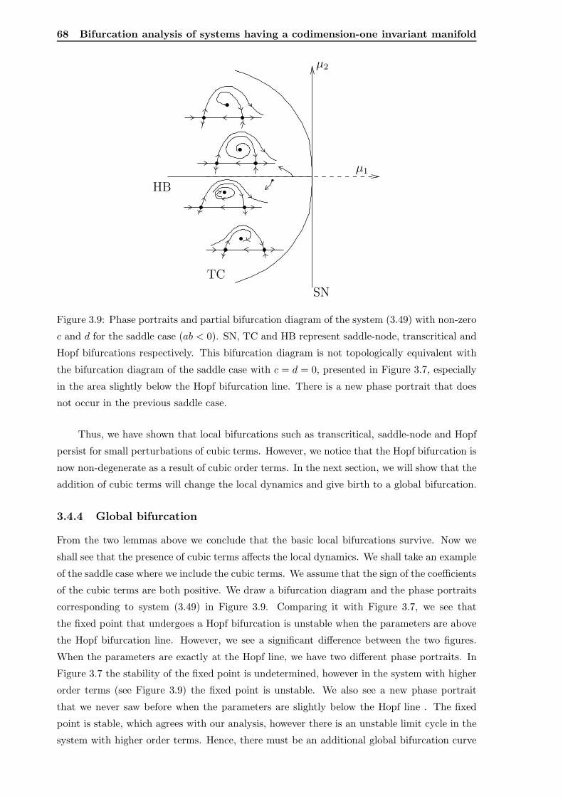
68 Bifurcation analysis of systems having a codimension-one invariant manifold
TC
SN
µ2
µ1
HB
Figure 3.9: Phase portraits and partial bifurcation diagram of the system (3.49) with non-zero
c and d for the saddle case (ab < 0). SN, TC and HB represent saddle-node, transcritical and
Hopf bifurcations respectively. This bifurcation diagram is not topologically equivalent with
the bifurcation diagram of the saddle case with c = d = 0, presented in Figure 3.7, especially
in the area slightly below the Hopf bifurcation line. There is a new phase portrait that does
not occur in the previous saddle case.
Thus, we have shown that local bifurcations such as transcritical, saddle-node and Hopf
persist for small perturbations of cubic terms. However, we notice that the Hopf bifurcation is
now non-degenerate as a result of cubic order terms. In the next section, we will show that the
addition of cubic terms will change the local dynamics and give birth to a global bifurcation.
3.4.4 Global bifurcation
From the two lemmas above we conclude that the basic local bifurcations survive. Now we
shall see that the presence of cubic terms affects the local dynamics. We shall take an example
of the saddle case where we include the cubic terms. We assume that the sign of the coefficients
of the cubic terms are both positive. We draw a bifurcation diagram and the phase portraits
corresponding to system (3.49) in Figure 3.9. Comparing it with Figure 3.7, we see that
the fixed point that undergoes a Hopf bifurcation is unstable when the parameters are above
the Hopf bifurcation line. However, we see a significant difference between the two figures.
When the parameters are exactly at the Hopf line, we have two different phase portraits. In
Figure 3.7 the stability of the fixed point is undetermined, however in the system with higher
order terms (see Figure 3.9) the fixed point is unstable. We also see a new phase portrait
that we never saw before when the parameters are slightly below the Hopf line . The fixed
point is stable, which agrees with our analysis, however there is an unstable limit cycle in the
system with higher order terms. Hence, there must be an additional global bifurcation curve
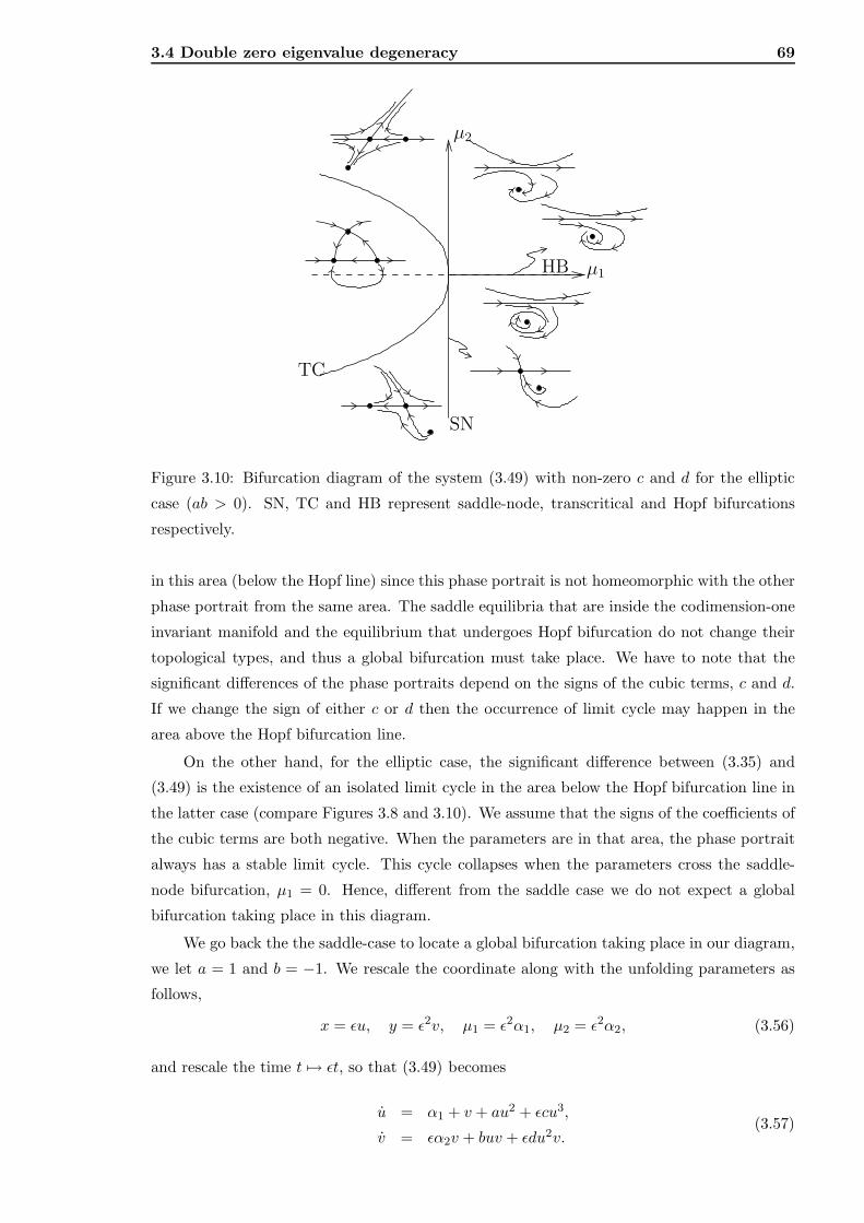
3.4 Double zero eigenvalue degeneracy 69
µ2
TC
SN
µ1HB
Figure 3.10: Bifurcation diagram of the system (3.49) with non-zero c and d for the elliptic
case (ab > 0). SN, TC and HB represent saddle-node, transcritical and Hopf bifurcations
respectively.
in this area (below the Hopf line) since this phase portrait is not homeomorphic with the other
phase portrait from the same area. The saddle equilibria that are inside the codimension-one
invariant manifold and the equilibrium that undergoes Hopf bifurcation do not change their
topological types, and thus a global bifurcation must take place. We have to note that the
significant differences of the phase portraits depend on the signs of the cubic terms, c and d.
If we change the sign of either c or d then the occurrence of limit cycle may happen in the
area above the Hopf bifurcation line.
On the other hand, for the elliptic case, the significant difference between (3.35) and
(3.49) is the existence of an isolated limit cycle in the area below the Hopf bifurcation line in
the latter case (compare Figures 3.8 and 3.10). We assume that the signs of the coefficients of
the cubic terms are both negative. When the parameters are in that area, the phase portrait
always has a stable limit cycle. This cycle collapses when the parameters cross the saddle-
node bifurcation, µ1 = 0. Hence, different from the saddle case we do not expect a global
bifurcation taking place in this diagram.
We go back the the saddle-case to locate a global bifurcation taking place in our diagram,
we let a = 1 and b = −1. We rescale the coordinate along with the unfolding parameters as
follows,
x = ǫu, y = ǫ2v, µ1 = ǫ2α1, µ2 = ǫ2α2, (3.56)
and rescale the time t 7→ ǫt, so that (3.49) becomes
u = α1 + v + au2 + ǫcu3,
v = ǫα2v + buv + ǫdu2v.(3.57)
70 Bifurcation analysis of systems having a codimension-one invariant manifold
Note that for ǫ = 0 we have a system that is completely integrable, with an integral as follows,
F (u, v) = −bv− 2ab (α1
2a+
v
2a− b+u2
2).
We take an example of the saddle case, where a = 1 and b = −1. Furthermore, without loss
of generality we set α1 = −1 since the case of interest occurs when µ1 < 0. The variation of
µ1 < 0 is obtained as ǫ varies. We now consider the system (3.57) multiplied by the integrating
factor vl−1 where l = −2a/b,
u = α1vl−1 + vl + au2vl−1 + ǫcu3vl−1,
v = buvl + ǫα2vl + ǫdu2vl.
(3.58)
The above system is a dilated version of the vector field (3.57) for v > 0, thus the solution
curves of (3.57) are topologically equivalent to those of (3.58). We would like to show that
for small ǫ and suitable choices of (α2, c, d), the isolated level curve (i.e. heteroclinic orbit) is
preserved. First we set the system above in a vector notation,
w = k(w) + ǫl(w, α2). (3.59)
Applying the Melnikov method and Green’s theorem, we deduce that given a closed curve Γ
we have∫
int Γtrace Dl(w, α2) dw = 0, (3.60)
for a chosen α2 where the trace of Dl is given by
trace Dl = vl−1(3cu2 + lα2 + dlu2); l = −2a/b. (3.61)
We automatically have trace Dk = 0, since it is integrable. We therefore must find a value, K
such that F−1(K) is a heteroclinic curve ΓK . It turns out that the value K = 0 corresponds to
the heteroclinic orbit. Gathering all the information above and the facts that we have a = 1,
b = −1 and α1 = −1, we have to integrate∫ ∫
int ΓK
[(3c + 2d)u2v + 2α2v]du dv, (3.62)
where the closed curve ΓK is given by
v2(−1
2+v
3+u2
2) = 0. (3.63)
Evaluating the integral above gives
12
5α2 +
18
35c+
12
35d = 0. (3.64)
This equation determines the location of the heteroclinic bifurcation in our parameter space
(up to order ǫ), and in terms of the variables used before scaling, we obtain the equation for
the heteroclinic bifurcation curve:
µ2 =(3c+ 2d)
14µ1 + O(ǫ). (3.65)
We have proven the following lemma.
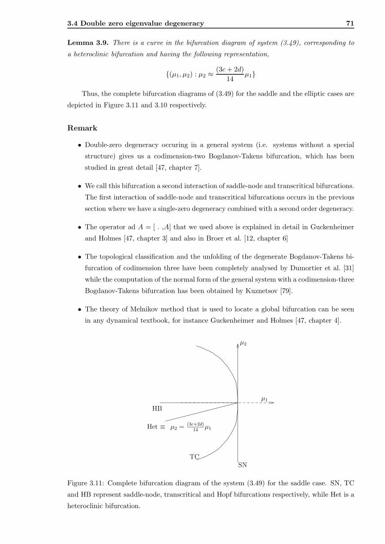
3.4 Double zero eigenvalue degeneracy 71
Lemma 3.9. There is a curve in the bifurcation diagram of system (3.49), corresponding to
a heteroclinic bifurcation and having the following representation,
{(µ1, µ2) : µ2 ≈ (3c + 2d)
14µ1}
Thus, the complete bifurcation diagrams of (3.49) for the saddle and the elliptic cases are
depicted in Figure 3.11 and 3.10 respectively.
Remark
• Double-zero degeneracy occuring in a general system (i.e. systems without a special
structure) gives us a codimension-two Bogdanov-Takens bifurcation, which has been
studied in great detail [47, chapter 7].
• We call this bifurcation a second interaction of saddle-node and transcritical bifurcations.
The first interaction of saddle-node and transcritical bifurcations occurs in the previous
section where we have a single-zero degeneracy combined with a second order degeneracy.
• The operator ad A = [ . ,A] that we used above is explained in detail in Guckenheimer
and Holmes [47, chapter 3] and also in Broer et al. [12, chapter 6]
• The topological classification and the unfolding of the degenerate Bogdanov-Takens bi-
furcation of codimension three have been completely analysed by Dumortier et al. [31]
while the computation of the normal form of the general system with a codimension-three
Bogdanov-Takens bifurcation has been obtained by Kuznetsov [79].
• The theory of Melnikov method that is used to locate a global bifurcation can be seen
in any dynamical textbook, for instance Guckenheimer and Holmes [47, chapter 4].
SN
µ2
µ1
HB
TC
Het ≡ µ2 = (3c+2d)14
µ1
Figure 3.11: Complete bifurcation diagram of the system (3.49) for the saddle case. SN, TC
and HB represent saddle-node, transcritical and Hopf bifurcations respectively, while Het is a
heteroclinic bifurcation.
72 Bifurcation analysis of systems having a codimension-one invariant manifold
3.5 A single-zero and a pair of purely imaginary eigenvalues
In this section, we provide an analysis of the remaining bifurcation of codimension-two that
occurs in a system having a codimension-one invariant manifold. We discuss the problem of
a single-zero and a pair of purely imaginary eigenvalues degeneracies. We work on a three-
dimensional system since we can reduce the dimension of the system by a center manifold
reduction. When we deal with a pair of purely imaginary eigenvalues, it is always convenient
to work in polar coordinates, which we will do in a moment. Moreover, we will see that we
can reduce the three-dimensional system into a two-dimensional system by removing the angle
part of our system under some assumptions. Thus, most of the analyse in this section are
mainly planar. We will translate some of the results we obtain in the planar analysis to the
three dimensional system. Some complex dynamics shall appear since some assumptions that
previously applied do not apply anymore.
The Jordan canonical form of the linear part of our system will be:
A =
0 −ω 0
ω 0 0
0 0 0
. (3.66)
Thus we have a three-dimensional system as follows,
x1 = −ωx2 + O(‖(x1, x2, y)‖2),
x2 = ωx1 + O(‖(x1, x2, y)‖2),
y = y(O(‖(x1, x2, y)‖)).
(3.67)
Using the method of normal form, we can remove some nonlinear terms in the equation above.
Moreover, the normal form can be conveniently written in the cylindrical polar coordinates as
follows,
r = a1ry + a2r3 + a3ry
2 + O(‖(r, y)‖4),
θ = ω + O(‖(r, y)‖2),
y = y(b1y + b2r2 + b3y
2 + O(‖(r, y)‖3)),
(3.68)
provided that all the normal form coefficients are non-zero. It turns out that the θ-dependence
in the r and y components of the vector field can be removed to order k for k arbitrarily large.
This is important since we can truncate our equation to some order and ignore the θ part of
our vector field. Then we perform a local bifurcation analysis on the r, y parts of the vector
field. In some sense, for r, y sufficiently small, the r− y plane can be thought of as a Poincare
map for the full three-dimensional system. We thus remove the θ part and truncate terms of
order four and higher,
r = a1ry + a2r3 + a3ry
2,
y = y(b1y + b2r2 + b3y
2).(3.69)
Before we do further analysis on the system above we shall do another transformation
that helps reduce the number of parameters we have. We introduce a new coordinate by the
following transformation:
s = r(1 + gy),
w = y + hr2 + iy2,
τ = (1 + jy)−1t,
(3.70)
3.5 A single-zero and a pair of purely imaginary eigenvalues 73
and compute the vector field (3.69) with respect to the new coordinate:
ds
dτ= a1sw + (a2 − a1h)s3 + (a3 + b1g − a1i+ a1j)sw
2 +Rs(s,w),
dw
dτ= b1w
2 + (b2 + 2a1h− 2b1h)s2w + (b3 + b1j)w3 +Rw(s,w). (3.71)
The remainder terms have order at least four in (s,w), hence we ignore these higher order
terms. We now choose (g, h, i, j) to make (3.71) as simple as possible. The new cubic co-
efficients introduced in the above system depend linearly on (g, h, i, j) as described by the
matrix:
M =
0 a1 0 0
−b1 0 a1 −a1
0 −2a1 + 2b1 0 0
0 0 0 −b1
, (3.72)
where v is (g, h, i, j) and Mv has the components (−a1h,−b1g+a1i−a1j,−2a1h+2b1h,−b1j)which is added to the components s3, sw2, s2w and w3. The matrix has rank three with a
kernel spanned by the vector (a1, 0, b1, 0). Consequently, we may choose v such that Mv
is equal to (0, a3, 0, b3) since this vector is in the range of M. Thus, we can assume that
the coefficients of sw2 and w3 are zero and consider only the cubic perturbation (s3, s2w) as
follows:r = a1ry + a2r
3,
y = y(b1y + b2r2).
(3.73)
3.5.1 Phase portraits of normal forms with a Hopf-zero degeneracy
We consider the equation (3.73) and scale the above system by the following transformation:
r = αr and y = βy. (3.74)
Then the equation (3.73) becomes
˙r = α(a1ryαβ
+ a2r3
α3 ),
˙y = y(b1yβ
+ b2r2
α2 .(3.75)
We set β = −b1 and α =√
|b2| and drop the bars, thus it yields
r = a1ry + a2r3,
y = y(−y + sr2),(3.76)
where s = ±1. The coefficients, a1, a2 are different from those of the equation (3.73), however
we keep the same notations for convenience. They can be positive or negative, but will be
assumed to be non-zero. We also need a1 − a2 6= 0 as will be explained below. We note that
we have two invariant manifolds in this case, one is y = 0 (our codimension-one invariant
manifold) and one is r = 0 as a result of the symmetry (r, y) 7→ (−r, y). Thus we only need
to consider half the r − y plane due to this symmetry. We also have another symmetry that
involves some parameters which is
(s, y, t, a2) 7→ −(s, y, t, a2). (3.77)
74 Bifurcation analysis of systems having a codimension-one invariant manifold
As a consequence, we can set s = −1 without further considering the case s = 1 since it
follows from the symmetry above.
We now want to classify the phase portraits of (3.76) near the origin. Consider the r− y
half plane, r ≥ 0 . We shall divide cases here, firstly we blow the area y > 0 up and then the
area y < 0. In the area y > 0, we perform the first blowing-up:
(r, y) 7→ (R,Y 2), (3.78)
leading to
R = a1RY2 + a2R
3,
Y = −12Y
3 − 12R
2Y.(3.79)
By means of polar blowing-up R = ρ cos θ and Y = ρ sin θ, we get:
ρ = ρ(a1 cos2 θ sin2 θ + a2 cos4 θ − 12 sin4 θ − 1
2 cos2 θ sin2 θ),
θ = − cos θ sin θ((a1 + 12) sin2 θ + (a2 + 1
2 ) cos2 θ),(3.80)
where ρ ≥ 0 and θ ∈ [0, π2 ].
There are three possible equilibria on ρ = 0, which are:
(i) ρ = 0, θ = 0, whose linearization matrix is:
J(0, 0) =
(
a2 0
0 −a2 − 12
)
,
(ii) ρ = 0, θ = π2 , whose linearization matrix is:
J(0,π
2) =
(
−12 0
0 a1 + 12
)
,
(iii) ρ = 0, θ = α, where α = arctan
√
−a1+ 1
2
a2+ 1
2
. The Jacobian matrix evaluated at this
equilibrium is
J(0, α) =
(
−12 0
0 (2a1+1)(2a2+1)2(a1−a2)
)
.
Hence there are six areas in the a1 − a2 plane that will yield qualitatively different phase
portraits of (3.80) which are
1. a1 > −12 ,a2 > 0,
2. a1 > −12 ,−1
2 < a2 < 0,
3. a1 > −12 ,a2 ≤ −1
2 ,
4. a1 ≤ −12 ,a2 > 0,
5. a1 ≤ −12 ,−1
2 < a2 < 0 and
6. a1 ≤ −12 ,a2 ≤ −1
2 .
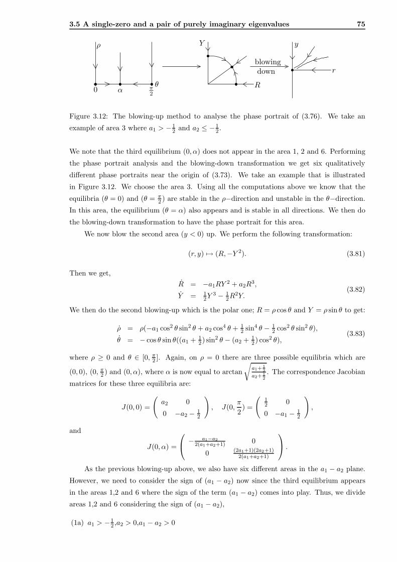
3.5 A single-zero and a pair of purely imaginary eigenvalues 75
0 α π
2
θ R
Y
r
y
blowing
down
ρ
Figure 3.12: The blowing-up method to analyse the phase portrait of (3.76). We take an
example of area 3 where a1 > −12 and a2 ≤ −1
2 .
We note that the third equilibrium (0, α) does not appear in the area 1, 2 and 6. Performing
the phase portrait analysis and the blowing-down transformation we get six qualitatively
different phase portraits near the origin of (3.73). We take an example that is illustrated
in Figure 3.12. We choose the area 3. Using all the computations above we know that the
equilibria (θ = 0) and (θ = π2 ) are stable in the ρ−direction and unstable in the θ−direction.
In this area, the equilibrium (θ = α) also appears and is stable in all directions. We then do
the blowing-down transformation to have the phase portrait for this area.
We now blow the second area (y < 0) up. We perform the following transformation:
(r, y) 7→ (R,−Y 2). (3.81)
Then we get,
R = −a1RY2 + a2R
3,
Y = 12Y
3 − 12R
2Y.(3.82)
We then do the second blowing-up which is the polar one; R = ρ cos θ and Y = ρ sin θ to get:
ρ = ρ(−a1 cos2 θ sin2 θ + a2 cos4 θ + 12 sin4 θ − 1
2 cos2 θ sin2 θ),
θ = − cos θ sin θ((a1 + 12) sin2 θ − (a2 + 1
2 ) cos2 θ),(3.83)
where ρ ≥ 0 and θ ∈ [0, π2 ]. Again, on ρ = 0 there are three possible equilibria which are
(0, 0), (0, π2 ) and (0, α), where α is now equal to arctan
√
a1+ 1
2
a2+ 1
2
. The correspondence Jacobian
matrices for these three equilibria are:
J(0, 0) =
(
a2 0
0 −a2 − 12
)
, J(0,π
2) =
(
12 0
0 −a1 − 12
)
,
and
J(0, α) =
− a1−a2
2(a1+a2+1) 0
0 (2a1+1)(2a2+1)2(a1+a2+1)
.
As the previous blowing-up above, we also have six different areas in the a1 − a2 plane.
However, we need to consider the sign of (a1 − a2) now since the third equilibrium appears
in the areas 1,2 and 6 where the sign of the term (a1 − a2) comes into play. Thus, we divide
areas 1,2 and 6 considering the sign of (a1 − a2),
(1a) a1 > −12 ,a2 > 0,a1 − a2 > 0
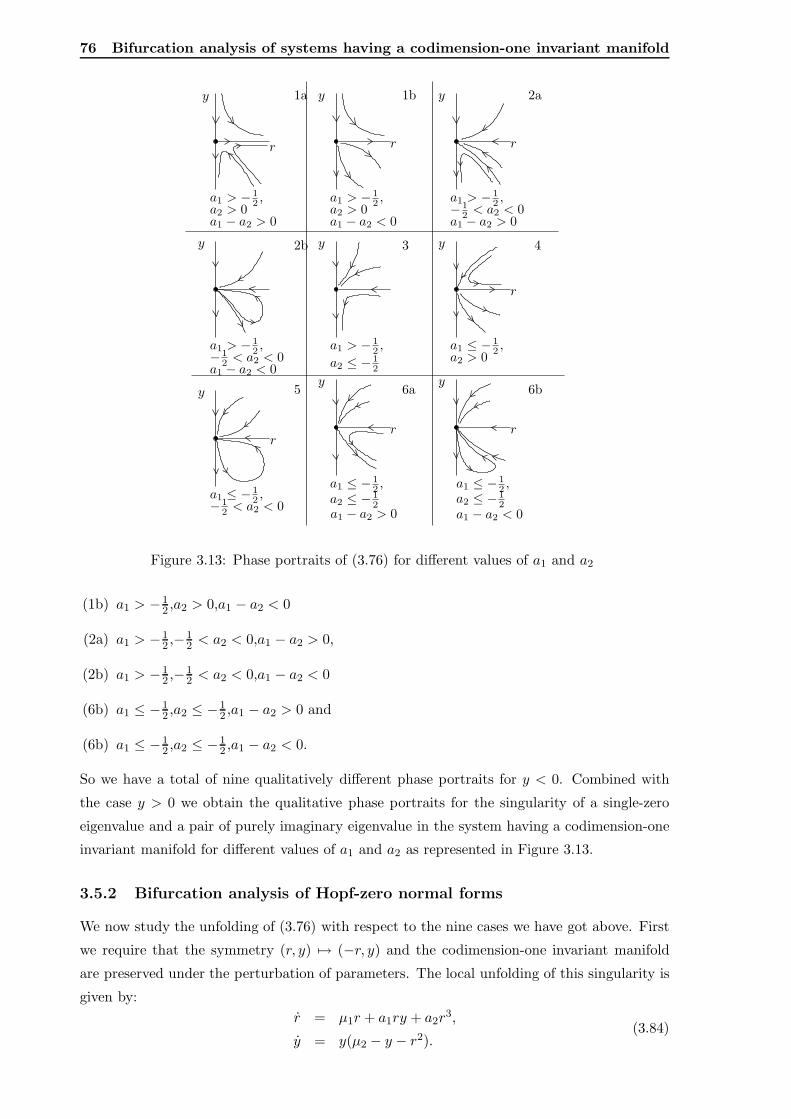
76 Bifurcation analysis of systems having a codimension-one invariant manifold
r
y y y
r r
a1 > − 1
2,a1 > − 1
2,
a2 > 0
a1 > − 1
2,
a2 > 0 − 1
2< a2 < 0
a1 − a2 > 0 a1 − a2 < 0 a1 − a2 > 0
y
− 1
2< a2 < 0
a1 > − 1
2,
a1 − a2 < 0
y y
r
a1 ≤ − 1
2,
a2 > 0
a1 ≤ − 1
2,
− 1
2< a2 < 0
y
rr
y
a1 ≤ − 1
2,
r
y
1a
2b
5
1b
3
6a
2a
4
6b
a1 > − 1
2,
a2 ≤ − 1
2
a1 ≤ − 1
2,
a1 − a2 > 0
a2 ≤ − 1
2
a1 − a2 < 0
a2 ≤ − 1
2
Figure 3.13: Phase portraits of (3.76) for different values of a1 and a2
(1b) a1 > −12 ,a2 > 0,a1 − a2 < 0
(2a) a1 > −12 ,−1
2 < a2 < 0,a1 − a2 > 0,
(2b) a1 > −12 ,−1
2 < a2 < 0,a1 − a2 < 0
(6b) a1 ≤ −12 ,a2 ≤ −1
2 ,a1 − a2 > 0 and
(6b) a1 ≤ −12 ,a2 ≤ −1
2 ,a1 − a2 < 0.
So we have a total of nine qualitatively different phase portraits for y < 0. Combined with
the case y > 0 we obtain the qualitative phase portraits for the singularity of a single-zero
eigenvalue and a pair of purely imaginary eigenvalue in the system having a codimension-one
invariant manifold for different values of a1 and a2 as represented in Figure 3.13.
3.5.2 Bifurcation analysis of Hopf-zero normal forms
We now study the unfolding of (3.76) with respect to the nine cases we have got above. First
we require that the symmetry (r, y) 7→ (−r, y) and the codimension-one invariant manifold
are preserved under the perturbation of parameters. The local unfolding of this singularity is
given by:
r = µ1r + a1ry + a2r3,
y = y(µ2 − y − r2).(3.84)
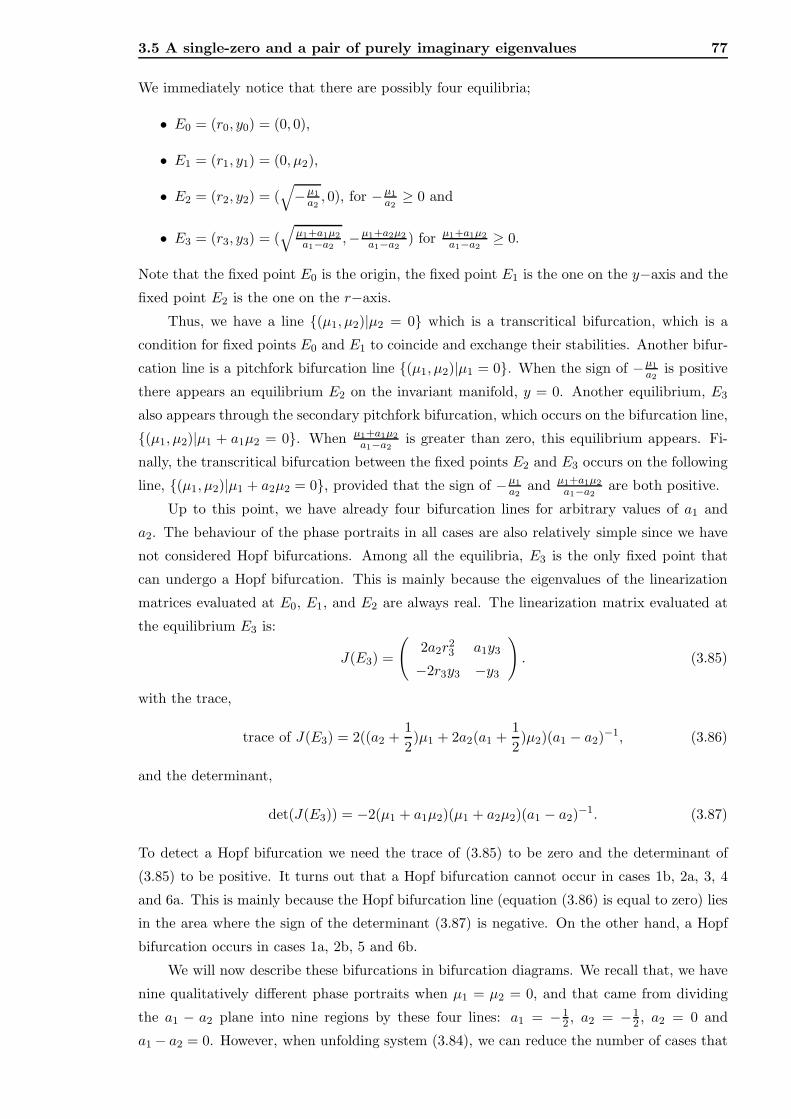
3.5 A single-zero and a pair of purely imaginary eigenvalues 77
We immediately notice that there are possibly four equilibria;
• E0 = (r0, y0) = (0, 0),
• E1 = (r1, y1) = (0, µ2),
• E2 = (r2, y2) = (√
−µ1
a2, 0), for −µ1
a2≥ 0 and
• E3 = (r3, y3) = (√
µ1+a1µ2
a1−a2,−µ1+a2µ2
a1−a2) for µ1+a1µ2
a1−a2≥ 0.
Note that the fixed point E0 is the origin, the fixed point E1 is the one on the y−axis and the
fixed point E2 is the one on the r−axis.
Thus, we have a line {(µ1, µ2)|µ2 = 0} which is a transcritical bifurcation, which is a
condition for fixed points E0 and E1 to coincide and exchange their stabilities. Another bifur-
cation line is a pitchfork bifurcation line {(µ1, µ2)|µ1 = 0}. When the sign of −µ1
a2is positive
there appears an equilibrium E2 on the invariant manifold, y = 0. Another equilibrium, E3
also appears through the secondary pitchfork bifurcation, which occurs on the bifurcation line,
{(µ1, µ2)|µ1 + a1µ2 = 0}. When µ1+a1µ2
a1−a2is greater than zero, this equilibrium appears. Fi-
nally, the transcritical bifurcation between the fixed points E2 and E3 occurs on the following
line, {(µ1, µ2)|µ1 + a2µ2 = 0}, provided that the sign of −µ1
a2and µ1+a1µ2
a1−a2are both positive.
Up to this point, we have already four bifurcation lines for arbitrary values of a1 and
a2. The behaviour of the phase portraits in all cases are also relatively simple since we have
not considered Hopf bifurcations. Among all the equilibria, E3 is the only fixed point that
can undergo a Hopf bifurcation. This is mainly because the eigenvalues of the linearization
matrices evaluated at E0, E1, and E2 are always real. The linearization matrix evaluated at
the equilibrium E3 is:
J(E3) =
(
2a2r23 a1y3
−2r3y3 −y3
)
. (3.85)
with the trace,
trace of J(E3) = 2((a2 +1
2)µ1 + 2a2(a1 +
1
2)µ2)(a1 − a2)−1, (3.86)
and the determinant,
det(J(E3)) = −2(µ1 + a1µ2)(µ1 + a2µ2)(a1 − a2)−1. (3.87)
To detect a Hopf bifurcation we need the trace of (3.85) to be zero and the determinant of
(3.85) to be positive. It turns out that a Hopf bifurcation cannot occur in cases 1b, 2a, 3, 4
and 6a. This is mainly because the Hopf bifurcation line (equation (3.86) is equal to zero) lies
in the area where the sign of the determinant (3.87) is negative. On the other hand, a Hopf
bifurcation occurs in cases 1a, 2b, 5 and 6b.
We will now describe these bifurcations in bifurcation diagrams. We recall that, we have
nine qualitatively different phase portraits when µ1 = µ2 = 0, and that came from dividing
the a1 − a2 plane into nine regions by these four lines: a1 = −12 , a2 = −1
2 , a2 = 0 and
a1 − a2 = 0. However, when unfolding system (3.84), we can reduce the number of cases that
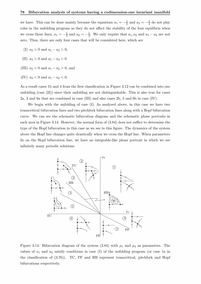
78 Bifurcation analysis of systems having a codimension-one invariant manifold
we have. This can be done mainly because the equations a1 = −12 and a2 = −1
2 do not play
roles in the unfolding program as they do not affect the stability of the four equilibria when
we cross these lines, a1 = −12 and a2 = −1
2 . We only require that a1, a2 and a1 − a2 are not
zero. Thus, there are only four cases that will be considered here, which are
(I) a2 > 0 and a1 − a2 > 0,
(II) a2 > 0 and a1 − a2 < 0
(III) a2 < 0 and a1 − a2 > 0, and
(IV) a2 < 0 and a1 − a2 < 0.
As a result cases 1b and 4 from the first classification in Figure 3.12 can be combined into one
unfolding (case (II)) since their unfolding are not distinguishable. This is also true for cases
2a, 3 and 6a that are combined in case (III) and also cases 2b, 5 and 6b in case (IV).
We begin with the unfolding of case (I). As analysed above, in this case we have two
transcritical bifurcation lines and two pitchfork bifurcation lines along with a Hopf bifurcation
curve. We can see the schematic bifurcation diagram and the schematic phase portraits in
each area in Figure 3.14. However, the normal form of (3.84) does not suffice to determine the
type of the Hopf bifurcation in this case as we see in this figure. The dynamics of the system
above the Hopf line changes quite drastically when we cross the Hopf line. When parameters
lie on the Hopf bifurcation line, we have an integrable-like phase portrait in which we see
infinitely many periodic solutions.
HB
µ2
TC
HB
PF
PF
µ1
TC
1
2
3
4
5
6
7
8
Figure 3.14: Bifurcation diagram of the system (3.84) with µ1 and µ2 as parameters. The
values of a1 and a2 satisfy conditions in case (I) of the unfolding program (or case 1a in
the classification of (3.76)). TC, PF and HB represent transcritical, pitchfork and Hopf
bifurcations respectively.
3.5 A single-zero and a pair of purely imaginary eigenvalues 79
We now turn to cases (II) and (III). These unfoldings are relatively simple since these
cases (1b, 2a, 3, 4 and 6a) do not undergo Hopf bifurcation in their unfoldings. One can see
the bifurcation diagrams for these cases in Figure 3.15 and Figure 3.16 respectively. These
bifurcation diagrams are depicted by assuming a1 > −12 , a2 > 0, a1 − a2 < 0 for case (II) and
a1− > 12 , a2 < 0, a1 − a2 > 0 for case (III).
Our final case, case (IV) which includes cases 2b, 5 and 6b in the classification of (3.76),
is rather complicated, as a Hopf bifurcation plays a role here. As noticed in the previous
analysis in case (I), the Hopf bifurcation in this case is degenerate. One can see that the
equilibrium E3 drastically changes from a stable fixed point to an unstable fixed point. The
dynamics around it also change significantly. It is mainly because, when the parameters µ1
and µ2 are on the Hopf bifurcation line, we have an integrable-like phase portrait where we
see infinitely many periodic solutions. This problem will disappear if we add other normal
form coefficients. We note that the fact that the Hopf bifurcation line lies inside the second
quadrant (µ1 < 0, µ2 > 0) is because we depict this schematic bifurcation diagram by assuming
a1 < −12 , a2 > −1
2 . If we vary a1 and a2, provided that we are still inside case (IV), we shall
have all the bifurcations that we had before, however the Hopf bifurcation will take place in
a different quadrant in the parameter space.
We now want to consider the effect of higher order terms. As those fixed points near
the origin are hyperbolic, they will persist for small perturbations from higher order terms as
µ2
PF
µ1
TC
PF
TC
1
2
3
4
5
6
7
Figure 3.15: Bifurcation diagram of the system (3.84) with µ1 and µ2 as parameters. The
values of a1 and a2 satisfy conditions in case (II) of the unfolding program (or case 1b and 4
in the classification of (3.76)). TC and PF represent transcritical and pitchfork bifurcations
respectively.
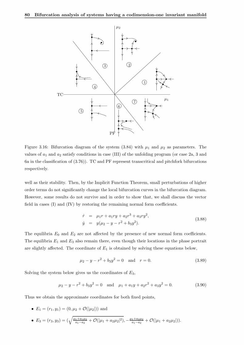
80 Bifurcation analysis of systems having a codimension-one invariant manifold
µ1
TC
PF
µ2
1
23
4
56
7
Figure 3.16: Bifurcation diagram of the system (3.84) with µ1 and µ2 as parameters. The
values of a1 and a2 satisfy conditions in case (III) of the unfolding program (or case 2a, 3 and
6a in the classification of (3.76)). TC and PF represent transcritical and pitchfork bifurcations
respectively.
well as their stability. Then, by the Implicit Function Theorem, small perturbations of higher
order terms do not significantly change the local bifurcation curves in the bifurcation diagram.
However, some results do not survive and in order to show that, we shall discuss the vector
field in cases (I) and (IV) by restoring the remaining normal form coefficients.
r = µ1r + a1ry + a2r3 + a3ry
2,
y = y(µ2 − y − r2 + b3y2).
(3.88)
The equilibria E0 and E2 are not affected by the presence of new normal form coefficients.
The equilibria E1 and E3 also remain there, even though their locations in the phase portrait
are slightly affected. The coordinate of E1 is obtained by solving these equations below,
µ2 − y − r2 + b3y2 = 0 and r = 0. (3.89)
Solving the system below gives us the coordinates of E3,
µ2 − y − r2 + b3y2 = 0 and µ1 + a1y + a2r
2 + a3y2 = 0. (3.90)
Thus we obtain the approximate coordinates for both fixed points,
• E1 = (r1, y1) = (0, µ2 + O(|µ2|)) and
• E3 = (r3, y3) = (√
µ1+a1µ2
a1−a2+ O(|µ1 + a2µ2|2),−µ1+a2µ2
a1−a2+ O(|µ1 + a2µ2|)).
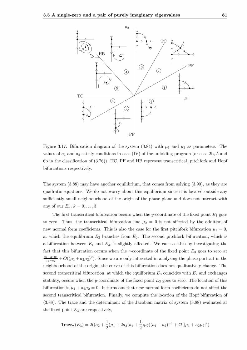
3.5 A single-zero and a pair of purely imaginary eigenvalues 81
1
23
4
5
6
7
8
TC
PF
µ2
µ1
TC
PF
HB
Figure 3.17: Bifurcation diagram of the system (3.84) with µ1 and µ2 as parameters. The
values of a1 and a2 satisfy conditions in case (IV) of the unfolding program (or case 2b, 5 and
6b in the classification of (3.76)). TC, PF and HB represent transcritical, pitchfork and Hopf
bifurcations respectively.
The system (3.88) may have another equilibrium, that comes from solving (3.90), as they are
quadratic equations. We do not worry about this equilibrium since it is located outside any
sufficiently small neighbourhood of the origin of the phase plane and does not interact with
any of our Ek, k = 0, . . . , 3.
The first transcritical bifurcation occurs when the y-coordinate of the fixed point E1 goes
to zero. Thus, the transcritical bifurcation line µ2 = 0 is not affected by the addition of
new normal form coefficients. This is also the case for the first pitchfork bifurcation µ1 = 0,
at which the equilibrium E2 branches from E0. The second pitchfork bifurcation, which is
a bifurcation between E1 and E3, is slightly affected. We can see this by investigating the
fact that this bifurcation occurs when the r-coordinate of the fixed point E3 goes to zero atµ1+a1µ2
a1−a2+O((µ1 +a2µ2)2). Since we are only interested in analysing the phase portrait in the
neighbourhood of the origin, the curve of this bifurcation does not qualitatively change. The
second transcritical bifurcation, at which the equilibrium E3 coincides with E2 and exchanges
stability, occurs when the y-coordinate of the fixed point E3 goes to zero. The location of this
bifurcation is µ1 + a2µ2 = 0. It turns out that new normal form coefficients do not affect the
second transcritical bifurcation. Finally, we compute the location of the Hopf bifurcation of
(3.88). The trace and the determinant of the Jacobian matrix of system (3.88) evaluated at
the fixed point E3 are respectively,
TraceJ(E3) = 2((a2 +1
2)µ1 + 2a2(a1 +
1
2)µ2)(a1 − a2)−1 + O(|µ1 + a2µ2|2)
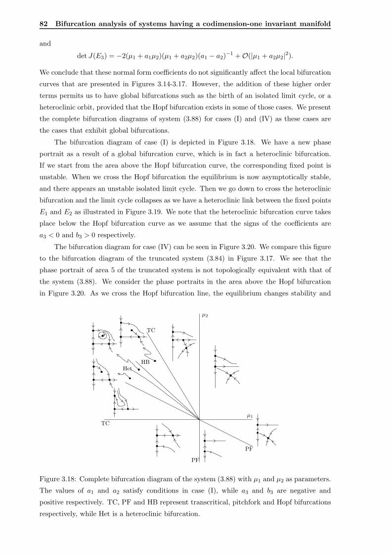
82 Bifurcation analysis of systems having a codimension-one invariant manifold
and
det J(E3) = −2(µ1 + a1µ2)(µ1 + a2µ2)(a1 − a2)−1 + O(|µ1 + a2µ2|2).
We conclude that these normal form coefficients do not significantly affect the local bifurcation
curves that are presented in Figures 3.14-3.17. However, the addition of these higher order
terms permits us to have global bifurcations such as the birth of an isolated limit cycle, or a
heteroclinic orbit, provided that the Hopf bifurcation exists in some of those cases. We present
the complete bifurcation diagrams of system (3.88) for cases (I) and (IV) as these cases are
the cases that exhibit global bifurcations.
The bifurcation diagram of case (I) is depicted in Figure 3.18. We have a new phase
portrait as a result of a global bifurcation curve, which is in fact a heteroclinic bifurcation.
If we start from the area above the Hopf bifurcation curve, the corresponding fixed point is
unstable. When we cross the Hopf bifurcation the equilibrium is now asymptotically stable,
and there appears an unstable isolated limit cycle. Then we go down to cross the heteroclinic
bifurcation and the limit cycle collapses as we have a heteroclinic link between the fixed points
E1 and E2 as illustrated in Figure 3.19. We note that the heteroclinic bifurcation curve takes
place below the Hopf bifurcation curve as we assume that the signs of the coefficients are
a3 < 0 and b3 > 0 respectively.
The bifurcation diagram for case (IV) can be seen in Figure 3.20. We compare this figure
to the bifurcation diagram of the truncated system (3.84) in Figure 3.17. We see that the
phase portrait of area 5 of the truncated system is not topologically equivalent with that of
the system (3.88). We consider the phase portraits in the area above the Hopf bifurcation
in Figure 3.20. As we cross the Hopf bifurcation line, the equilibrium changes stability and
µ2
TC
HB
PF
PF
µ1
TC
Het
Figure 3.18: Complete bifurcation diagram of the system (3.88) with µ1 and µ2 as parameters.
The values of a1 and a2 satisfy conditions in case (I), while a3 and b3 are negative and
positive respectively. TC, PF and HB represent transcritical, pitchfork and Hopf bifurcations
respectively, while Het is a heteroclinic bifurcation.
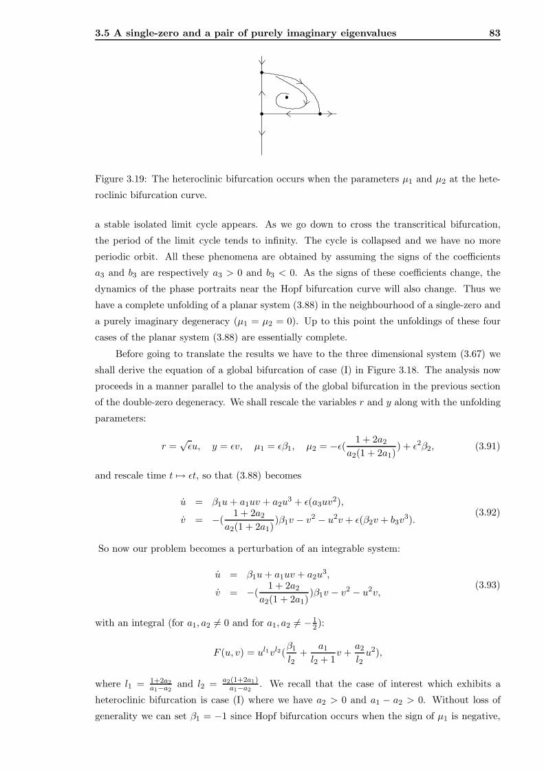
3.5 A single-zero and a pair of purely imaginary eigenvalues 83
Figure 3.19: The heteroclinic bifurcation occurs when the parameters µ1 and µ2 at the hete-
roclinic bifurcation curve.
a stable isolated limit cycle appears. As we go down to cross the transcritical bifurcation,
the period of the limit cycle tends to infinity. The cycle is collapsed and we have no more
periodic orbit. All these phenomena are obtained by assuming the signs of the coefficients
a3 and b3 are respectively a3 > 0 and b3 < 0. As the signs of these coefficients change, the
dynamics of the phase portraits near the Hopf bifurcation curve will also change. Thus we
have a complete unfolding of a planar system (3.88) in the neighbourhood of a single-zero and
a purely imaginary degeneracy (µ1 = µ2 = 0). Up to this point the unfoldings of these four
cases of the planar system (3.88) are essentially complete.
Before going to translate the results we have to the three dimensional system (3.67) we
shall derive the equation of a global bifurcation of case (I) in Figure 3.18. The analysis now
proceeds in a manner parallel to the analysis of the global bifurcation in the previous section
of the double-zero degeneracy. We shall rescale the variables r and y along with the unfolding
parameters:
r =√ǫu, y = ǫv, µ1 = ǫβ1, µ2 = −ǫ( 1 + 2a2
a2(1 + 2a1)) + ǫ2β2, (3.91)
and rescale time t 7→ ǫt, so that (3.88) becomes
u = β1u+ a1uv + a2u3 + ǫ(a3uv
2),
v = −(1 + 2a2
a2(1 + 2a1))β1v − v2 − u2v + ǫ(β2v + b3v
3).(3.92)
So now our problem becomes a perturbation of an integrable system:
u = β1u+ a1uv + a2u3,
v = −(1 + 2a2
a2(1 + 2a1))β1v − v2 − u2v,
(3.93)
with an integral (for a1, a2 6= 0 and for a1, a2 6= −12):
F (u, v) = ul1vl2(β1
l2+
a1
l2 + 1v +
a2
l2u2),
where l1 = 1+2a2
a1−a2and l2 = a2(1+2a1)
a1−a2. We recall that the case of interest which exhibits a
heteroclinic bifurcation is case (I) where we have a2 > 0 and a1 − a2 > 0. Without loss of
generality we can set β1 = −1 since Hopf bifurcation occurs when the sign of µ1 is negative,
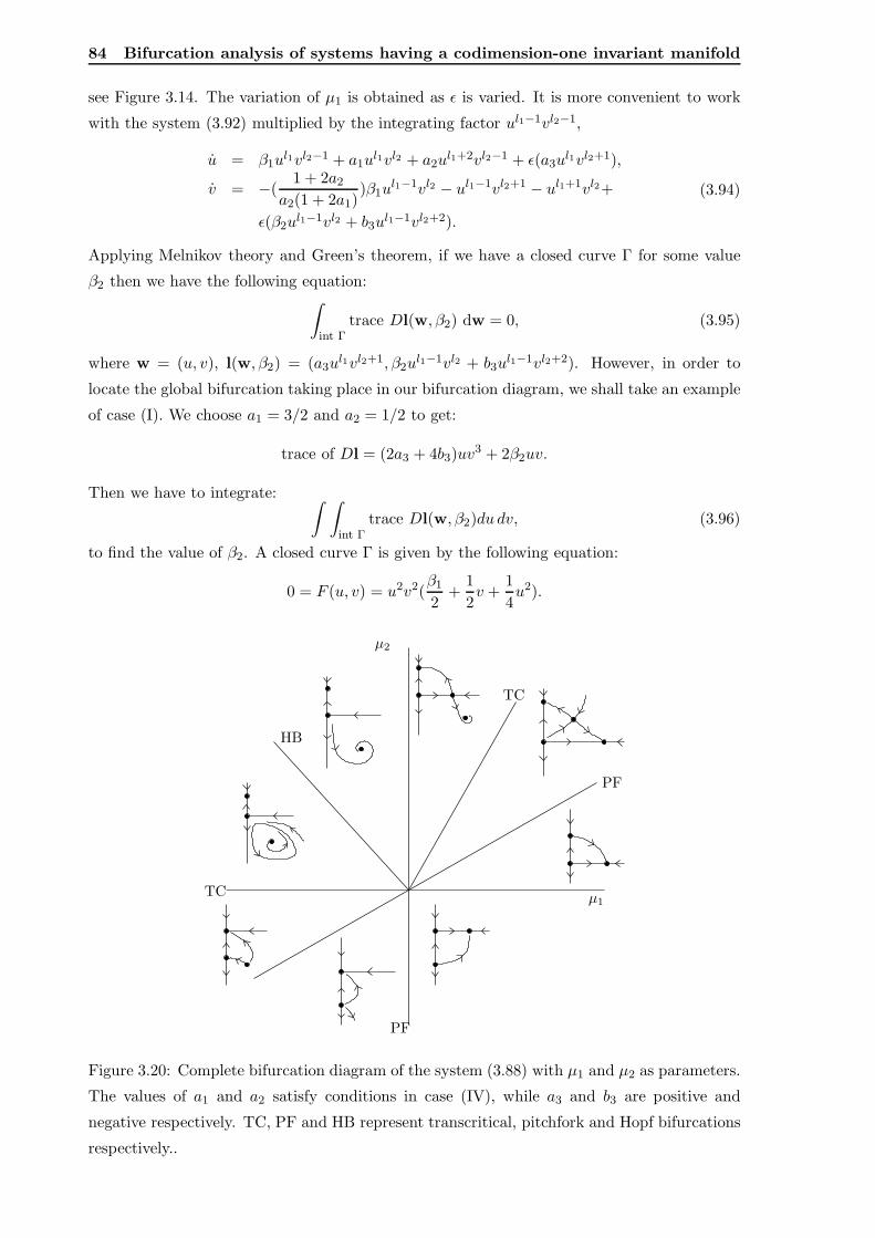
84 Bifurcation analysis of systems having a codimension-one invariant manifold
see Figure 3.14. The variation of µ1 is obtained as ǫ is varied. It is more convenient to work
with the system (3.92) multiplied by the integrating factor ul1−1vl2−1,
u = β1ul1vl2−1 + a1u
l1vl2 + a2ul1+2vl2−1 + ǫ(a3u
l1vl2+1),
v = −(1 + 2a2
a2(1 + 2a1))β1u
l1−1vl2 − ul1−1vl2+1 − ul1+1vl2+
ǫ(β2ul1−1vl2 + b3u
l1−1vl2+2).
(3.94)
Applying Melnikov theory and Green’s theorem, if we have a closed curve Γ for some value
β2 then we have the following equation:∫
int Γtrace Dl(w, β2) dw = 0, (3.95)
where w = (u, v), l(w, β2) = (a3ul1vl2+1, β2u
l1−1vl2 + b3ul1−1vl2+2). However, in order to
locate the global bifurcation taking place in our bifurcation diagram, we shall take an example
of case (I). We choose a1 = 3/2 and a2 = 1/2 to get:
trace of Dl = (2a3 + 4b3)uv3 + 2β2uv.
Then we have to integrate:∫ ∫
int Γtrace Dl(w, β2)du dv, (3.96)
to find the value of β2. A closed curve Γ is given by the following equation:
0 = F (u, v) = u2v2(β1
2+
1
2v +
1
4u2).
TC
PF
µ2
µ1
TC
PF
HB
Figure 3.20: Complete bifurcation diagram of the system (3.88) with µ1 and µ2 as parameters.
The values of a1 and a2 satisfy conditions in case (IV), while a3 and b3 are positive and
negative respectively. TC, PF and HB represent transcritical, pitchfork and Hopf bifurcations
respectively..
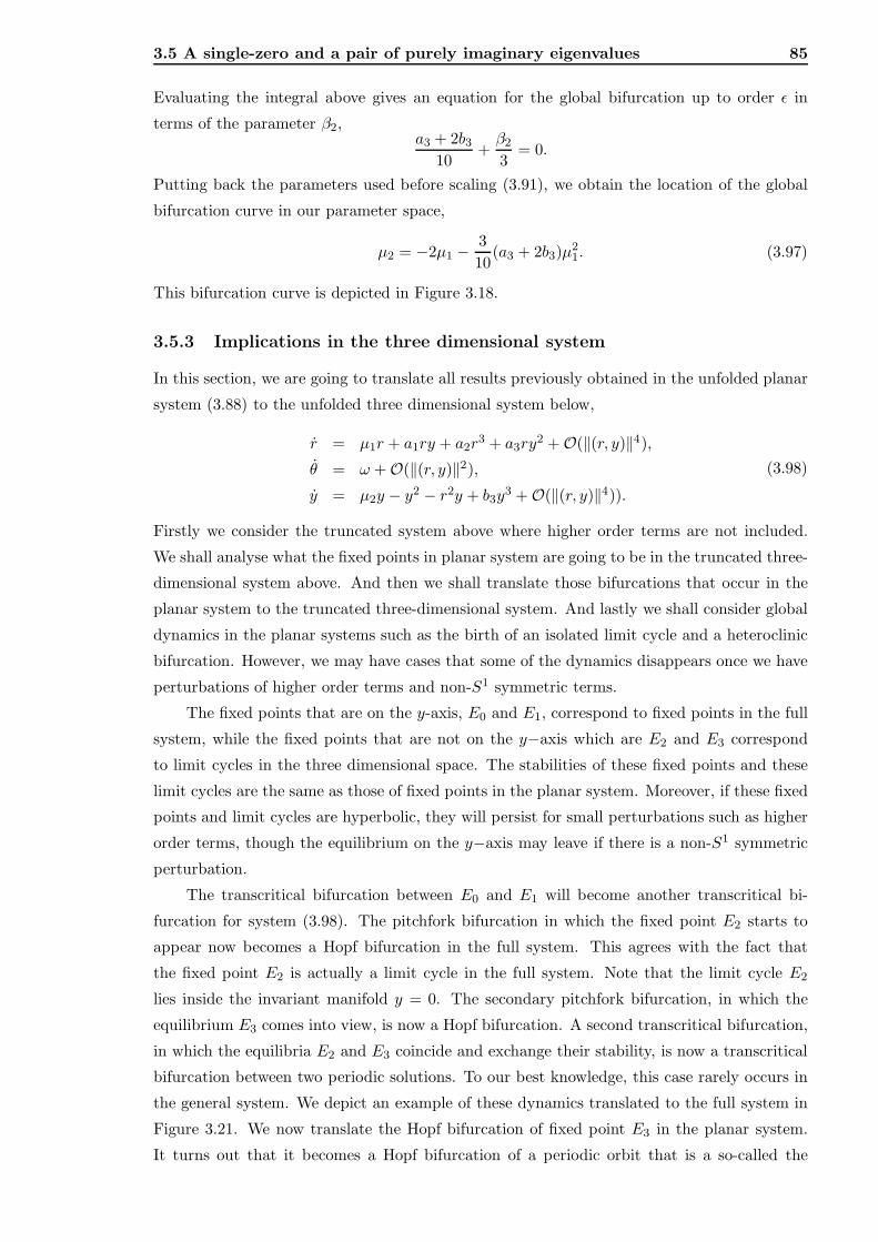
3.5 A single-zero and a pair of purely imaginary eigenvalues 85
Evaluating the integral above gives an equation for the global bifurcation up to order ǫ in
terms of the parameter β2,a3 + 2b3
10+β2
3= 0.
Putting back the parameters used before scaling (3.91), we obtain the location of the global
bifurcation curve in our parameter space,
µ2 = −2µ1 −3
10(a3 + 2b3)µ2
1. (3.97)
This bifurcation curve is depicted in Figure 3.18.
3.5.3 Implications in the three dimensional system
In this section, we are going to translate all results previously obtained in the unfolded planar
system (3.88) to the unfolded three dimensional system below,
r = µ1r + a1ry + a2r3 + a3ry
2 + O(‖(r, y)‖4),
θ = ω + O(‖(r, y)‖2),
y = µ2y − y2 − r2y + b3y3 + O(‖(r, y)‖4)).
(3.98)
Firstly we consider the truncated system above where higher order terms are not included.
We shall analyse what the fixed points in planar system are going to be in the truncated three-
dimensional system above. And then we shall translate those bifurcations that occur in the
planar system to the truncated three-dimensional system. And lastly we shall consider global
dynamics in the planar systems such as the birth of an isolated limit cycle and a heteroclinic
bifurcation. However, we may have cases that some of the dynamics disappears once we have
perturbations of higher order terms and non-S1 symmetric terms.
The fixed points that are on the y-axis, E0 and E1, correspond to fixed points in the full
system, while the fixed points that are not on the y−axis which are E2 and E3 correspond
to limit cycles in the three dimensional space. The stabilities of these fixed points and these
limit cycles are the same as those of fixed points in the planar system. Moreover, if these fixed
points and limit cycles are hyperbolic, they will persist for small perturbations such as higher
order terms, though the equilibrium on the y−axis may leave if there is a non-S1 symmetric
perturbation.
The transcritical bifurcation between E0 and E1 will become another transcritical bi-
furcation for system (3.98). The pitchfork bifurcation in which the fixed point E2 starts to
appear now becomes a Hopf bifurcation in the full system. This agrees with the fact that
the fixed point E2 is actually a limit cycle in the full system. Note that the limit cycle E2
lies inside the invariant manifold y = 0. The secondary pitchfork bifurcation, in which the
equilibrium E3 comes into view, is now a Hopf bifurcation. A second transcritical bifurcation,
in which the equilibria E2 and E3 coincide and exchange their stability, is now a transcritical
bifurcation between two periodic solutions. To our best knowledge, this case rarely occurs in
the general system. We depict an example of these dynamics translated to the full system in
Figure 3.21. We now translate the Hopf bifurcation of fixed point E3 in the planar system.
It turns out that it becomes a Hopf bifurcation of a periodic orbit that is a so-called the
86 Bifurcation analysis of systems having a codimension-one invariant manifold
E0
E1
E2
E3
y
r E0
E1
y
y = 0
Figure 3.21: Three-dimensional flow with respect to the flow in planar system. We see that
E0 and E1 stay as fixed points and E2 and E3 become periodic solutions.
Neimark-Sacker bifurcation. Furthermore, the closed orbit in the planar system represents
an invariant torus in the three-dimensional system. The heteroclinic link that is depicted in
Figure 3.19 corresponds to a half sphere in the full system.
Recall that the previous implications for the three-dimensional system concern the trun-
cated system (3.98) where we do not have the perturbation of the higher order terms. The
addition of higher order terms does not affect the existence and the stability of the fixed points
and the periodic orbits for sufficiently small ||(µ1, µ2)|| because of the fact that they are hyper-
bolic. Then, by using the Implicit Function Theorem for a sufficiently small neighbourhood
of (µ1, µ2) = (0, 0), higher order terms do not affect the local bifurcation curves which are
transcritical, Hopf and Neimark-Sacker bifurcations. However, adding higher-order terms will
result in topologically non-equivalent bifurcation diagrams as the truncated system has some
degenerate features that disappear under perturbations by these higher order terms.
Let us first explain a simple case that is sensitive to the addition of higher order terms.
Consider the phase portrait of case (II), depicted in Figure 3.15 in area 2. It has two saddle-
type equilibria on the y−axis. This axis in fact is invariant due to the S1 symmetry that
connects the one-dimensional stable manifold of one fixed point to the one-dimensional unsta-
ble manifold of the other; thus we have a heteroclinic link for all values of µ1 and µ2 in this
region. The addition of general higher-order terms or in particular, the addition of non-S1
symmetric terms will make the link disappear. Thus, generically we do not have a heteroclinic
link between these two fixed points. We note that this phenomenon does not occur only in
case (II) but also in all cases where we have two saddle-type equilibria on the y−axis.
The other dynamics that most likely disappears is the global bifurcation phenomenon.
Let us consider the heteroclinic orbit in Figure 3.19. We know that in R3 the heteroclinic
link becomes a sphere that is cut in half by the codimension-one invariant manifold possessed
by the system. The half sphere is formed by the two-dimensional unstable manifold of the
fixed point E1 and the two-dimensional stable manifold of the fixed point E2. Thus this
half sphere is a result of two surfaces perfectly coinciding. This is an extremely degenerate
structure that most likely disappears when higher order terms are added. Generally either we
have no intersection at all between these two-dimensional manifolds or, we have a transversal
3.6 Discussion 87
intersection of these manifolds which leads to a transversal heteroclinic orbit in the three
dimensional system.
The other phenomenon that previously did not occur and is now possible is the Shilnikov
homoclinic bifurcation. Let us consider the fixed point E1 in Figure 3.19. The addition of
higher order terms can destroy the S1 symmetry, thus the y− axis is no longer invariant.
Then the stable manifold of this fixed point, which previously lies inside the y−axis, can
coincide with the unstable manifold of the same fixed point forming a homoclinic orbit. This
bifurcation can possibly lead to exotic dynamics such as chaotic dynamics.
As we discussed earlier, an invariant torus appears through a non-degenerate Neimark-
Sacker bifurcation. Under a variation of parameters, a quasi-periodic orbit is born and dies,
this is called a phase locking of a periodic orbit. This is another exotic dynamics that can
be investigated. To end this discussion we note that we do not prove the existence of these
dynamics, we only mention that the dynamics described above can possibly occur.
Remarks
• The single-zero combined with a purely imaginary degeneracy that occurs in the general
system gives us the Fold-Hopf bifurcation. The truncated system of this degeneracy
is studied in great detail in many bifurcation text books [78]. The reader can also
read more information about the implications of the truncated system for the full three
dimensional system in these books.
• The blowing-up method that we used in this section was first introduced by Takens [116].
That paper provided the blowing-up for a double-zero, a single-zero combined with a
pair of purely imaginary, and two pairs of purely imaginary cases. This method is
also explained in great detail in Broer et al. [12] in which polar blowing-up as well as
directional blowing-up is discussed. In the discussion in this chapter, we have performed
a successive polar and directional blowing-ups.
• In 1969, Shilnikov described a bifurcation involving a homoclinic orbit from a saddle-type
equilibrium. Shilnikov proved that the existence of such an orbit, commonly referred to
as the Shilnikov homoclinic bifurcation, leads to the existence of infinitely many periodic
orbits, i.e. a route to chaos. A good reconstruction of Shilnikov bifurcation from the
single-zero combined with a purely imaginary degeneracy is explained in great detail in
Wiggins [126]. The Shilnikov bifurcation is also found in an application [120].
• The problem of a quasi-periodic orbit on the surface of an invariant torus of the Fold-
Hopf bifurcation has been studied by Scheurle and Marsden [109]. The reconstruction
of such a quasi-periodic orbit is explained in Kuznetsov [78, chapter 7].
3.6 Discussion
In this chapter, we showed that the bifurcations of a system with a special structure (i.e. a
codimension-one invariant manifold) are different from those of a general dynamical system.
88 Bifurcation analysis of systems having a codimension-one invariant manifold
We showed that a codimension-one invariant manifold structure gives rise to many interesting
bifurcations, which in particular are one codimension-one bifurcation and three codimension-
two bifurcations. This number is less than the number of bifurcations of a general dynamical
system, due to the restriction imposed by the special structure. For each bifurcation, the
normal form of a system with a codimension-one invariant manifold is derived and treated
by the same methods as the normal form of a general dynamical system. Thus, most of
the analysis of each bifurcation here is analogous to the analysis of bifurcations of a general
dynamical system.
Our results can be applied directly to a system that possesses the same special structure
which is a codimension-one invariant manifold. We also require that this manifold is preserved
under a variation of parameters. One system that has this special structure is actually dis-
cussed in chapter three of this thesis, i.e. the two-dimensional Lotka-Volterra system with a
constant term. The result of this chapter explains why the Lotka-Volterra system has two
unusual bifurcations in the first place.
We recall that there are two saddle-node–transcritical interactions in the Lotka-Volterra
system with a constant term. The first interaction that is a single-zero eigenvalue with higher
order term degeneracy is discussed in section three of this chapter. This is also true for the
second interaction that has a double-zero eigenvalue degeneracy. This is discussed in section
four.
It is true that this chapter has not discussed the Lotka-Volterra system with constant
terms. However, if we think about it one more time, we have discussed something that is
much more general than the Lotka-Volterra system with constant terms. We have discussed
a general system that has a special structure that is actually possessed by the Lotka-Volterra
system with constant terms. Thus in this sense, we have done a global analysis in which the
Lotka-Volterra system is included.
We remark that the problem in the single-zero and the pair of purely imaginary eigen-
values degeneracy is an interesting topic for future research. In our analysis, the full system
is reduced to a planar system featuring many interesting bifurcations. We can translate those
bifurcations to the full system which is three-dimensional, which leads to the occurrence of
bifurcations that are known to exist in three-dimensional vector fields but are not described
by the planar approximation. It will be an interesting challenge to study the existence of such
bifurcations.
CHAPTER 4
First integrals of Lotka Volterrasystems with constant terms
4.1 Introduction
Consider a general dynamical system in n−dimensions as follows
x = f(x, µ), x ∈ Rn with n > 1, (4.1)
where µ ∈ Rp is a parameter. Our main objective is to find conditions on the parameters such
that the system above possesses a first integral. In this chapter, we concentrate on finding
integrals of Lotka-Volterra systems with constant terms.
The Lotka-Volterra (LV) system has been the subject of intensive study during the past
century. The interaction of two species in an ecosystem [58], a metamorphosis of turbulence
in plasma physics [7], hydrodynamic equations, autocatalytic chemical reactions and many
more, are of Lotka-Volterra type. Given that there are many applications based on such
systems, it is important to understand the dynamics of Lotka-Volterra systems. Nevertheless,
the dynamics of such systems is far from being understood. Thus, our main motivation to
find first integrals of Lotka-Volterra systems or any dynamical system is the fact that first
integrals give global information about the long-term behaviour of such systems.
In two-dimensional systems, the existence of a first integral implies that the system is
completely integrable because the phase portraits are completely characterized. For three-
dimensional systems, the existence of a first integral means that the system cannot have
chaotic motions as the solution will live inside the level sets of such an integral function. The
existence of a second integral gives a completely integrable case.
Many different methods have been developed to study the existence of first integrals of
Lotka-Volterra systems. Perhaps, one of the earliest attempts to study the existence of first
integrals was Cairo et al. [18] who studied the integrability of n-dimensional Lotka-Volterra
equations using the Carleman embedding method. They sought a constant of motion (i.e.
invariant) that may be either time-dependent or time-independent. There is also Cairo and
90 First integrals of Lotka Volterra systems with constant terms
Llibre [24] who used a polynomial inverse integrating factor to find a condition for the existence
of the first integral. The Darboux method that uses the relationship between algebraic curves
and integrability of differential equations has been introduced by Cairo and Llibre [22] to
study two-dimensional Lotka-Volterra systems. Cairo et al. (1999) [20] also used the same
method to search for a first integral of two-dimensional quadratic systems.
In the three-dimensional case, the Darboux method has also been used to derive an
integral for three-dimensional Lotka-Volterra systems [14] and for the so-called ABC systems,
which correspond to particular cases of three-dimensional Lotka-Volterra systems where the
linear and the diagonal terms are absent. The ABC systems were among the first three-
dimensional models that were investigated. One of the first studies was by Grammaticos et
al. in 1990 [46] in which the authors derived first integrals using the Frobenius Integrabilty
Theorem method (first introduced by Strelcyn and Wojciechowski [115]). Ollagnier [96] has
found polynomial first integrals of the ABC system.
Gao and Liu 1998 [39] presented a method that basically relies on changing variables to
transform three-dimensional Lotka-Volterra systems to two-dimensional ones. The existence
of first integrals follows from integrating the two-dimensional systems. Gao [37] used a direct
integration method to find first integrals of three-dimensional Lotka-Volterra systems. A new
algorithm presented by Gonzalez-Gascon and Peralta Salas [43] also used three-dimensional
Lotka-Volterra systems as an example of their method to find first integrals.
Other intensive research on finding first integrals is using the idea of associating a Hamil-
tonian to a first integral of a vector field. It was introduced by Nutku [100]. A generalization
of this idea to two-dimensional vector fields having a first integral was provided by Cairo and
Feix [16], in which through time rescaling the first integral can be considered as a Hamiltonian.
Using this relation, Cairo et al. [19] and Hua et al. [63] used an Ansatz for their Hamiltonian
functions. They assumed that a first integral (or an invariant) H is a product of two (or
three) functions, H = P (x, y)(Q(x, y))µ(R(x, y))ν . Subsequently, they derived conditions for
two-dimensional quadratic systems to have a first integral.
Another Hamiltonian method that has been used is as follows. A general system (4.1) is
said to have a Hamiltonian structure if and only if it can be written as x = f(x) = S(x)∇H(x),
where S is a skew-symmetric matrix and H is a smooth function. The matrix function S
must satisfy the Jacobi identity [38]. Plank [102] has used this property to find a Hamiltonian
function for two-dimensional Lotka-Volterra systems, while Gao [38], using the same property,
has derived conditions for three-dimensional systems not to be chaotic.
However in this chapter, we are not going to use the Jacobi identity property for the
matrix S since what we only need is the fact that H is a first integral, thus the fact that f(x)
can be written as S(x)∇H(x) is enough for us now. Consider the following proposition.
Proposition 4.10 (McLachlan et al. 1999 [94]). Let f ∈ Cr(Rn,Rn), r ≥ 1, n > 1, be a
vector field and H ∈ C(Rn,R) is a first integral of the vector field f (i.e. f.∇H = 0) for all
x. Then there is a skew-symmetric matrix function S(x) on the domain {x : ∇H 6= 0} such
that f = S∇H.
As a consequence of the proposition above, there is also a skew symmetric matrix function
4.2 Two-dimensional LV systems with constant terms 91
T (x) on the domain {x : f 6= 0} such that ∇H = Tf . We are going to use this idea to find
first integrals and their constraints for two- and three-dimensional Lotka-Volterra systems
with constant terms. We call the matrix T an integrating factor matrix. As the function H
is a first integral, we must have curl(∇H) = 0. This implies that
curl(Tf ) = 0. (4.2)
The above condition will be a condition for a matrix T to be an integrating factor. Making
an Ansatz concerning the integrating factor matrix T , we obtain both integrals as well as
conditions on the parameters for the existence of the integrals. However, the meaning of curl
will be different in every dimension greater than one. For two dimensional systems, curl(Tf)
will be just a scalar as follows,
∂(Tf)1∂x2
− ∂(Tf)2∂x1
= 0,
where (TF )i is the i− th component of the vector Tf . In three-dimensional systems, curl(Tf)
is a vector in R3, as a result of a cross product of the vectors ∇ and Tf .
We shall use the integrating factor matrix to find first integrals and their conditions. In-
tegrability of two-dimensional Lotka-Volterra systems with constant terms will be investigated
in the next section. Conditions and integrals are derived using an Ansatz on the integrating
factor matrix. First integrals of three-dimensional Lotka-Volterra systems are discussed in
section three. Finally, some remarks comparing known methods and our method to find first
integrals, along with a conclusion and suggestions for future research, are discussed in section
four. Note that we have not (yet) recovered all known integrals of LV systems with constant
terms, so there is still plenty to be done.
4.2 Two-dimensional LV systems with constant terms
In this section, we consider integrals of the two-dimensional Lotka-Volterra system with con-
stant terms:
x1 = f1(x1, x2) = x1(b1 + a11x1 + a12x2) + e1,
x2 = f2(x1, x2) = x2(b2 + a21x1 + a22x2) + e2, (4.3)
where bi, aij (i, j = 1, 2) are arbitrary parameters and e1, e2 are the constant terms. We
choose an integrating factor matrix as follows,
T (x1, x2) =
(
0 −αRαR 0
)
, α ∈ R, (4.4)
where we make the Ansatz that R = R(x1, x2) = xl1−11 xl2−1
2 , l1 and l2 are free parameters
that are to be determined later on. The matrix T (x1, x2) is an integrating factor if and only
if the curl of T f is zero, where f = (f1, f2). As is mentioned before, in the two dimensional
case, this condition is equivalent to the following,
∂(αRf1)
∂x1+∂(αRf2)
∂x2= 0. (4.5)
92 First integrals of Lotka Volterra systems with constant terms
The associated first integral H is given by
H(x1, x2) =
∫
R(x1, x2)f1(x1, x2) dx2 + h(x1), (4.6)
where h(x1) is found by imposing ∂H/∂x1 = −Rf2.
We then multiply the matrix (4.4) and the right-hand side of the vector field (4.3) and
substitute them in the equation (4.5) to get,
0 = xl1−11 xl2−1
2 [b1l1 + b2l2 + (l1a11 + l2a21 + a11)x1+ (4.7)
(l1a12 + l2a22 + a22)x2 + (l1 − 1)e/x1 + (l2 − 1)f/x2].
The expression above is satisfied if and only if the parameters satisfy these five conditions:
e1l1 = e1, (4.8)
e2l2 = e2, (4.9)
l1a11 + l2a21 = −a11, (4.10)
l1a12 + l2a22 = −a22, (4.11)
b1l1 + b2l2 = 0. (4.12)
We can write (4.8-4.12) as an overdetermined linear system:
Al = r, (4.13)
where l = (l1, l2) and the matrix A and the vector r are to be determined later. The system
has a solution only if the vector r is orthogonal to the left null space of the matrix A. In
the following we give the corresponding equations along with the resulting integrals for the
cases e1, e2 6= 0, e1 6= 0, e2 = 0 and e1 = e2 = 0 separately. The case e1 = 0, e2 6= 0 follows
by symmetry considerations. We note that the final case, which corresponds to the original
Lotka-Volterra system where e1 = e2 = 0, has been discussed by various people. However we
shall also discuss this case in order for the presentation to be self-contained.
4.2.1 The case e1, e2 6= 0
We have the case where both the constant terms e1 and e2 are non-zero. Then by (4.8) and
(4.9), this implies that l1 = l2 = 1. Moreover, we can simplify the other conditions to:
b1 + b2 = 0, 2a11 + a21 = 0, and a12 + 2a22 = 0. (4.14)
If the Lotka-Volterra system (4.3) with non-zero constant terms e and f satisfies conditions
(4.14), then it has a first integral that is given by:
H = b1x1x2 + a11x2
1 x2 − a22x1x2
2 + e1x2 − e2x1. (4.15)
4.2 Two-dimensional LV systems with constant terms 93
4.2.2 The case e1 6= 0, e2 = 0
One of the constant terms, e1 is not zero. This means that the free parameter l1 must be 1
by (4.8). We now have a linear system like (4.13) with a 3 by 1 matrix A and a vector r in
R3 with only one unknown l2. Without loss of generality, we assume that the matrix A is of
rank 1, when A has rank zero we have a trivial integral H = x2 since x2 = 0. Using the fact
that this system must be solvable, we can again find the conditions for the existence of the
first integral. First we assume that a21 6= 0. In that case the solvability conditions are given
by:2a11a22
a21− a22 − a12 = 0, and 2b2a11 − b1a21 = 0. (4.16)
If we have a21 = 0 and a22 6= 0 then we can compute the solvability conditions:
b2a22
(a22 + a12) − b1 = 0, and a11 = 0. (4.17)
Finally, when a21 = a22 = 0 but b2 6= 0 the solvability conditions are given by:
a22 + a12 = 0, and a11 = 0. (4.18)
Hence when our system satisfies one of the conditions above, there exists a unique solution,
l2. If l2 is not zero then the first integral is given by:
H = x l22 (−b2x1 −
a21
2x 2
1 − a22x1x2 +e1l2
). (4.19)
However, in the case where the exponent l2 is zero, the integral is given by:
H = −b2x1 −a21
2x 2
1 − a22x1x2 + e1 ln |x2|. (4.20)
4.2.3 The case e1 = 0 and e2 = 0
Finally, if e1 = e2 = 0 equations (4.8) and (4.9) are trivial and we have a linear system of the
form (4.13) with a 3 by 2 matrix A and a vector e in R3 from (4.10-4.12).
If A is of maximal rank then the solvability condition of the linear system (4.13) is given
by :
b1a22(a21 − a11) + b2a11(a12 − a22) = 0. (4.21)
So if our system satisfies the condition above, then there exist l1 and l2. When neither l1 and
l2 are zero, the first integral is given by:
H = x l11 x l2
2 (b1l2
+a11
l2x1 −
a22
l1x2). (4.22)
However, either l1 or l2 may be zero and if l1 = 0, l2 6= 0 and l2 6= −1 then we have
b2 = a22 = 0, a11 6= a21 and an integral that is given by:
H = x l22 (
b1l2
+a11
l2x1 +
a12
(l2 + 1)x2). (4.23)
But when l1 = 0 and l2 = −1, this implies b2 = 0 and a21 = a11. It follows that the integral
is given by:
H = a12 ln |x2| − a22 ln |x1| −b1x2
− a11x1
x2. (4.24)
94 First integrals of Lotka Volterra systems with constant terms
Finally, when both l1 and l2 are zero, which implies a11 = a22 = 0, the first integral is given
by:
H = b1 ln |x2| + a12x2 − b2 ln |x1| − a21x1. (4.25)
We remark that the case when l2 = 0, l1 6= 0, l1 6= −1 and the case when l2 = 0, l1 = −1
follow by symmetry considerations.
If matrix A has rank 1, we can assume without loss of generality that one of its column
vectors, (a11, a12, b1)T does not have zero norm and the other is proportional to it, namely:
(a21, a22, b2)T = λ(a11, a12, b1)T , (4.26)
where λ ∈ R. The solvability conditions depend very much on this vector. We summarize in
the following:
• if a11 6= 0, then the solvability conditions are b1 = 0 and a12 = a22. The integral is given
by
H = x2x−1
1 . (4.27)
• If a11 = 0 and a12 6= 0, then the solvability condition is b1 = 0 with the integral:
H = x2x−λ
1 , (4.28)
where λ = a22/a12.
• if a11 = 0, a12 6= 0 and b1 6= 0, then we need a22 = 0. The integral for this case is of the
form,
H = x2. (4.29)
• Finally if a11 = a12 = 0 but b1 6= 0 (since rank of A is one) then the system is already
solvable with the following integral:
H = x2x−λ
1 , (4.30)
where λ = b2/b1.
4.2.4 Further notes regarding the known integrals of two-dimensional LV
systems and quadratic systems
As we said earlier, many attempts have been made to study the integrability of two-dimensional
Lotka-Volterra systems and quadratic systems. Many people found different first integrals us-
ing different methods, and it may be possible that the first integral they found is similar to
the ones we have found in this discussion.
The first integral (4.15) along with its conditions (4.14) has been found before. It has been
found for the first time perhaps by Frommer (1934) (see Artes and Llibre (1994) [5]). Cairo
et al. [19] used the Hamiltonian method to derive first integrals for two-dimensional quadratic
systems and one of their results corresponds to the first integral (4.15). Hua et al. [64] studied
the connection between the existence of a first integral and the Painleve property in a general
4.3 Three-dimensional LV systems with constant terms 95
quadratic system. They listed first integrals of quadratic systems that have been found before
and (4.15) is one of them. The form of the first integral and the vector field they studied are
different, but through some invertible transformations it is not hard to check that they are
actually equivalent.
For the first integral in the case e1 = 0 and e2 = 0, it is not possible to list all the first
integrals that have been already derived since there are so many. First integrals (4.22-4.25)
have been derived by, for instance Nutku (1989), Cairo and Feix [15], Plank [102], Cairo and
Llibre (1999) [20] and (2000) [24] using various methods. We remark that the first integral
(4.25) that has constrains a11 = a22 = 0 was firstly derived by Volterra himself as a constant
of motion, (see the book by Hofbauer and Sigmund (1998) [58]). The other first integrals to
our best knowledge, for the cases where e1 6= 0, e2 = 0 and e1 = e2 = 0, seem to be new.
4.3 Three-dimensional LV systems with constant terms
We consider the following three-dimensional Lotka-Volterra systems with constant terms:
x1 = f1(x1, x2, x3) = x1(b1 + a11x1 + a12x2 + a13x3) + e1,
x2 = f2(x1, x2, x3) = x2(b2 + a21x1 + a22x2 + a23x3) + e2,
x3 = f3(x1, x2, x3) = x3(b3 + a31x1 + a32x2 + a33x3) + e3, (4.31)
where bi, aij (i, j = 1, 2) are arbitrary parameters and ei (i = 1, 2, 3) are the constant terms.
In this section, in order to find integrals of the system above we shall make the following two
Ansatzs for the skew-symmetric matrix T ,
T1(x1, x2, x3) = R
0 −α′ −β′
α′ 0 −γ′
β′ γ′ 0
, (4.32)
respectively,
T2(x1, x2, x3) = R
0 −αx3 −βx2
αx3 0 −γx1
βx2 γx1 0
, (4.33)
where α,α′, β, β′, γ, γ′ ∈ R are arbitrary parameters. The function R that we use here has
the same form that we have used in the two-dimensional case which is R = R(x1, x2, x3) =
xl1−11 xl2−1
2 xl3−13 , li (i = 1, 2, 3) are free parameters that are to be determined later on. The
matrices Ti(x1, x2, x3) (i = 1, 2) are integrating factors if and only if the curls of Tif are zero,
where f = (f1, f2, f3). In the three-dimensional case, this condition is equivalent to
∣
∣
∣
∣
∣
∣
∣
∣
i j k
∂/∂x1 ∂/∂x2 ∂/∂x3
∂Hi/∂x1 ∂Hi/∂x2 ∂Hi/∂x3
∣
∣
∣
∣
∣
∣
∣
∣
= 0, (4.34)
where
∇Hi = Tif (i = 1, 2). (4.35)
96 First integrals of Lotka Volterra systems with constant terms
We expand the above expression with respect to the matrices T1 and T2 as follows,
∂H1
∂x1= −Rα′f2 −Rβ′f3, (4.36)
∂H1
∂x2= Rα′f1 −Rγ′f3, (4.37)
∂H1
∂x3= Rβ′f1 +Rγ′f2. (4.38)
respectively
∂H2
∂x1= −Rαx3f2 −Rβx2f3, (4.39)
∂H2
∂x2= Rαx3f1 −Rγx1f3, (4.40)
∂H2
∂x3= Rβx2f1 +Rγx1f2. (4.41)
The associated first integral H1(x1, x2, x3), which corresponds to the matrix T1, is given by
H1(x1, x2, x3) =
∫
(Rβ′f1 +Rγ′f2) dx3 + h(x1, x2), (4.42)
where h(x1, x2) is found by imposing (4.36) and (4.37). Respectively, the associated first
integral in the case where we use the integrating factor matrix T2 can be found in a similar
way.
In the following, we shall derive integrals for the cases e1, e2, e3 6= 0; e1, e2 6= 0, e3 = 0;
e1 6= 0, e2 = e3 = 0; and e1 = e2 = e3 = 0.
4.3.1 The case e1, e2, e3 6= 0
We first start discussing the case where all the constant terms, e1, e2, e3 are not zero. We start
with the following lemma, which implies that the integrating factor matrix T2 does not work
in this case.
Lemma 4.11. If e1e2e3 6= 0 then we must have T2 = 0 in order to satisfy condition (4.34)
for the case that the subscript i = 2.
Proof. We substitute the expression (4.39-4.41) in the condition (4.34) for the case that the
subscript i = 2. Therefore, we have the following,
∂
∂x2(Rβx2f1 +Rγx1f2) − ∂
∂x3(Rαx3f1 −Rγx1f3)
∂
∂x3(−Rαx3f2 −Rβx2f3) − ∂
∂x1(Rβx2f1 +Rγx1f2)
∂
∂x1(Rαx3f1 −Rγx1f3) − ∂
∂x2(−Rαx3f2 −Rβx2f3)
= 0. (4.43)
We then substitute the differential equation (4.31) in the vector above. The first entry, which
has to be equal to zero, is equivalent to
0 = xl11 x
l2−12 xl3−1
3 [β(l2b1 + l2a11x1 + (l2 + 1)a12x2 + l2a13x3 + l2e1/x1)
+ γ(l2b2 + l2a21x1 + (l2 + 1)a22x2 + l2a23x3 + (l2 − 1)e2/x2)
− α(l3b1 + l3a11x1 + l3a12x2 + (l3 + 1)a13x3 + l3e1/x1)
+ γ(l3b3 + l3a31x1 + l3a32x2 + (l3 + 1)a33x3 + (l3 − 1)e3/x3)]. (4.44)
4.3 Three-dimensional LV systems with constant terms 97
The fact that the second entry of the vector (4.43) is equal to zero, gives us the following
equation,
0 = −xl1−11 xl2
2 xl3−13 [α(l3b2 + l3a21x1 + l3a22x2 + (l3 + 1)a23x3 + l3e2/x2)
+ β(l3b3 + l3a31x1 + l3a32x2 + (l3 + 1)a33x3 + (l3 − 1)e3/x3)
+ β(l1b1 + (l1 + 1)a11x1 + l1a12x2 + l1a13x3 + (l1 − 1)e1/x1)
+ γ(l1b2 + (l1 + 1)a21x1 + l1a22x2 + l1a23x3 + l1e2/x2)]. (4.45)
Finally, the fact that the third entry of the vector (4.43) is equal to zero, gives us the following
equation,
0 = xl1−11 xl2−1
2 xl33 [α(l1b1 + (l1 + 1)a11x1 + l1a12x2 + l1a13x3 + (l1 − 1)e1/x1)
− γ(l1b3 + (l1 + 1)a31x1 + l1a32x2 + l1a33x3 + l1e3/x3)
+ α(l2b2 + l2a21x1 + (l2 + 1)a22x2 + l2a23x3 + (l2 − 1)e2/x2)
+ β(l2b3 + l2a31x1 + (l2 + 1)a32x2 + l2a33x3 + l2e3/x3). (4.46)
We now want to find conditions on the parameters (α, β, γ, li, aij , bi, ei) such that the above
conditions are satisfied. If e1e2e3 6= 0, then it immediately follows that l1 = l2 = l3 = 1. Also,
from coefficients of 1/x1, 1/x2, and 1/x3 of (4.44-4.46) respectively, we have the following,
βe1l2 − αe1l3 = 0,
−αe2l3 − γe2l1 = 0,
−γe3l1 + βe3l2 = 0.
As e1e2e3 6= 0 and l1 = l2 = l3 = 1, we conclude that
β − α = 0,
α+ γ = 0,
−γ + β = 0,
which implies that α = β = γ = 0. Thus T2 has to be a zero matrix.
Therefore, we shall use the integrating factor matrix T1 to derive integrals for the case
e1e2e3 6= 0. We substitute the expressions (4.36-4.38) in the condition (4.34) for i = 1 and we
conclude that the following vector must be equal to zero.
∂
∂y(Rβ′f1 +Rγ′f2) − ∂
∂z(Rα′f1 −Rγ′f3)
∂
∂z(−Rα′f2 −Rβ′f3) − ∂
∂x(Rβ′f1 +Rγ′f2)
∂
∂x(Rα′f1 −Rγ′f3) − ∂
∂y(−Rα′f2 −Rβ′f3)
= 0. (4.47)
We substitute the vector field (4.31) into the above vector. The equation in the following is
due to the first entry of the above vector being equal to zero.
xl1−11 xl2−1
2 xl3−13
(
β′x1
x2[(l2 − 1)b1 + (l2 − 1)a11x1 + l2a12x2 + (l2 − 1)a13x3
98 First integrals of Lotka Volterra systems with constant terms
+(l2 − 1)e1x1
] + γ′[l2b2 + l2a21x1 + (l2 + 1)a22x2 + l2a23x3 + (l2 − 1)e2x2
]
−α′x1
x3[(l3 − 1)b1 + (l3 − 1)a11x1 + (l3 − 1)a12x2 + l3a13x3 + (l3 − 1)
e1x1
]
+γ′[l3b3 + l3a31x1 + l3a32x2 + (l3 + 1)a33x3 + (l3 − 1)e3x3
]
)
= 0. (4.48)
Substituting f1, f2 and f3 of the vector field (4.31) to the second entry of the vector (4.47),
we get the following,
−xl1−11 xl2−1
2 xl3−13
(
α′x2
x3[(l3 − 1)b2 + (l3 − 1)a21x1 + (l3 − 1)a22x2 + l3a23x3
+(l3 − 1)e2x2
] + β′[l3b3 + l3a31x1 + l3a32x2 + (l3 + 1)a33x3 + (l3 − 1)e3x3
]
+γ′x2
x1[(l1 − 1)b2 + l1a21x1 + (l1 − 1)a22x2 + (l1 − 1)a23x3 + (l1 − 1)
e2x2
]
+β′[l1b1 + (l1 + 1)a11x1 + l1a12x2 + l1a13x3 + (l1 − 1)e1x1
]
)
= 0. (4.49)
Finally, the fact that the third entry of the vector (4.47) is equal to zero gives,
xl1−11 xl2−1
2 xl3−13
(
−γ′x3
x1[(l1 − 1)b3 + l1a31x1 + (l1 − 1)a32x2 + (l1 − 1)a33x3
+(l1 − 1)e3x3
] + α′[l1b1 + (l1 + 1)a11x1 + l1a12x2 + l1a13x3 + (l1 − 1)e1x1
]
+β′x3
x2[(l2 − 1)b3 + (l2 − 1)a31x1 + l2a32x2 + (l2 − 1)a33x3 + (l2 − 1)
e3x3
]
+α′[l2b2 + l2a21x1 + (l2 + 1)a22x2 + l2a23x3 + (l2 − 1)e2x2
]
)
= 0. (4.50)
We now want to find conditions on the parameters (α′, β′, γ′, li, aij , bi, ei) such that the above
equations are satisfied. The results for this case are summarized in the following lemma.
Lemma 4.12. The vector field (4.31) with e1, e2, e3 6= 0 has a first integral in the following
cases:
1. if the conditions b1 + b2 = 0, 2a11 + a21 = 0, 2a22 + a12 = 0, a13 = a23 = 0 are satisfied,
then the integral is given by
H = b1x1x2 + a11x21x2 − a22x1x
22 + e1x2 − e2x1, (4.51)
2. if the conditions b1 + b2 = 0, b1 + b3 = 0, 2a11 + a21 = 0, 2a11 + a31 = 0, 2a22 + a12 = 0,
2a33 + a13 = 0, and a12a13 + a12a23 + a13a32 = 0 are satisfied then the integral is given
by
H = − 2b1a33x1x3 − 2b1a22x1x2 − 2a11a33x21x3 + 2a11a22x
21x2
+ 2a233x1x
23 + 2a2
22x1x22 + 4a22a33x1x2x3
+ 2(e3a33 + e2a22)x1 − 2e1a33x3 + 2e1a22x2, (4.52)
4.3 Three-dimensional LV systems with constant terms 99
3. if the conditions bi = 0 and aij = −2ajj for i 6= j and i, j = 1, 2, 3 are satisfied, then the
integral is given by
H = a211a22x
21x2 − a2
11a33x21x3 − a11a
222x1x
22 + a11a
233x1x
23 + a2
22a33x22x3
− a22a233x2x
23 + (−a11a22e2 + a11a33e3)x1 + (a11a22e1 − a22a33e3)x2
+ (a22a33e2 − a11a33e1)x3. (4.53)
Proof. It immediately follows from (4.48-4.50) that l1, l2, l3 must all equal to one. Conse-
quently, we get the following conditions on the parameters,
α′(b1 + b2) = 0, (4.54)
β′(b1 + b3) = 0, (4.55)
γ′(b2 + b3) = 0, (4.56)
α′(2a11 + a21) = 0, (4.57)
α′(2a22 + a12) = 0, (4.58)
β′(2a11 + a31) = 0, (4.59)
β′(2a33 + a13) = 0, (4.60)
γ′(2a22 + a32) = 0, (4.61)
γ′(2a33 + a23) = 0, (4.62)
−α′a13 + β′a12 + γ′(a21 + a31) = 0, (4.63)
α′a23 + β′(a12 + a32) + γ′a21 = 0, (4.64)
α′(a13 + a23) + β′a32 − γ′a31 = 0. (4.65)
1. We start with the case where α′ 6= 0, β′ = γ′ = 0. From (4.54-4.65) the following
conditions immediately apply:
b1 + b2 = 0, 2a11 + a21 = 0, (4.66)
2a22 + a12 = 0, a13 = a23 = 0, (4.67)
and using (4.42) we obtain the first integral (4.51).
2. We turn to the case where α′, β′ 6= 0, γ′ = 0. From (4.54-4.62), the following conditions
immediately apply,
b1 + b2 = 0, 2a11 + a21 = 0, 2a11 + a31 = 0, (4.68)
b1 + b3 = 0, 2a22 + a12 = 0, 2a33 + a13 = 0. (4.69)
While, α′ and β′ can be computed from the following linear homogeneous equations due
to (4.63-4.65),
α′a13 − β′a12 = 0, (4.70)
α′a23 + β′(a12 + a32) = 0, (4.71)
α′(a13 + a23) + β′a32 = 0. (4.72)
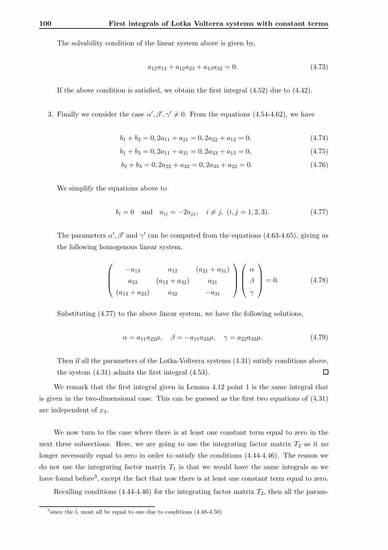
100 First integrals of Lotka Volterra systems with constant terms
The solvability condition of the linear system above is given by,
a12a13 + a12a23 + a13a32 = 0. (4.73)
If the above condition is satisfied, we obtain the first integral (4.52) due to (4.42).
3. Finally we consider the case α′, β′, γ′ 6= 0. From the equations (4.54-4.62), we have
b1 + b2 = 0, 2a11 + a21 = 0, 2a22 + a12 = 0, (4.74)
b1 + b3 = 0, 2a11 + a31 = 0, 2a33 + a13 = 0, (4.75)
b2 + b3 = 0, 2a22 + a32 = 0, 2a33 + a23 = 0. (4.76)
We simplify the equations above to
bi = 0 and aij = −2ajj, i 6= j, (i, j = 1, 2, 3). (4.77)
The parameters α′, β′ and γ′ can be computed from the equations (4.63-4.65), giving us
the following homogenous linear system,
−a13 a12 (a21 + a31)
a23 (a12 + a32) a21
(a13 + a23) a32 −a31
α
β
γ
= 0. (4.78)
Substituting (4.77) to the above linear system, we have the following solutions,
α = a11a22µ, β = −a11a33µ, γ = a22a33µ. (4.79)
Then if all the parameters of the Lotka-Volterra systems (4.31) satisfy conditions above,
the system (4.31) admits the first integral (4.53).
We remark that the first integral given in Lemma 4.12 point 1 is the same integral that
is given in the two-dimensional case. This can be guessed as the first two equations of (4.31)
are independent of x3.
We now turn to the case where there is at least one constant term equal to zero in the
next three subsections. Here, we are going to use the integrating factor matrix T2 as it no
longer necessarily equal to zero in order to satisfy the conditions (4.44-4.46). The reason we
do not use the integrating factor matrix T1 is that we would have the same integrals as we
have found before3, except the fact that now there is at least one constant term equal to zero.
Recalling conditions (4.44-4.46) for the integrating factor matrix T2, then all the param-
3since the li must all be equal to one due to conditions (4.48-4.50)
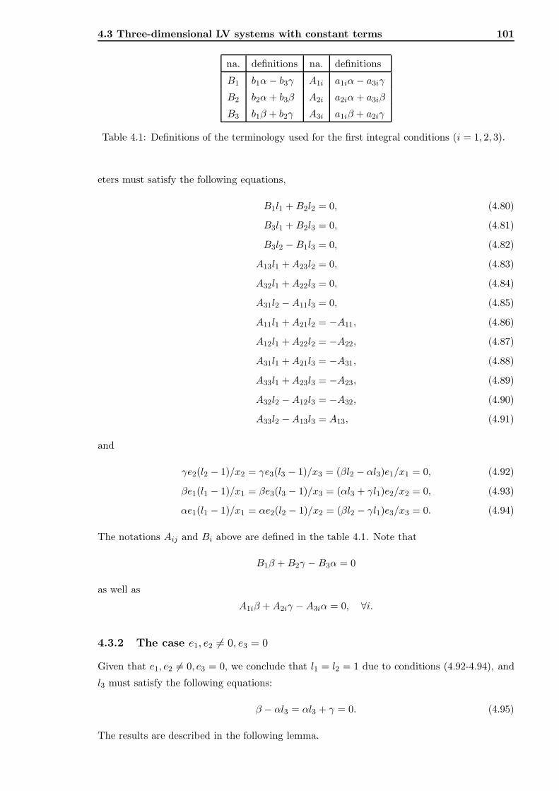
4.3 Three-dimensional LV systems with constant terms 101
na. definitions na. definitions
B1 b1α− b3γ A1i a1iα− a3iγ
B2 b2α+ b3β A2i a2iα+ a3iβ
B3 b1β + b2γ A3i a1iβ + a2iγ
Table 4.1: Definitions of the terminology used for the first integral conditions (i = 1, 2, 3).
eters must satisfy the following equations,
B1l1 +B2l2 = 0, (4.80)
B3l1 +B2l3 = 0, (4.81)
B3l2 −B1l3 = 0, (4.82)
A13l1 +A23l2 = 0, (4.83)
A32l1 +A22l3 = 0, (4.84)
A31l2 −A11l3 = 0, (4.85)
A11l1 +A21l2 = −A11, (4.86)
A12l1 +A22l2 = −A22, (4.87)
A31l1 +A21l3 = −A31, (4.88)
A33l1 +A23l3 = −A23, (4.89)
A32l2 −A12l3 = −A32, (4.90)
A33l2 −A13l3 = A13, (4.91)
and
γe2(l2 − 1)/x2 = γe3(l3 − 1)/x3 = (βl2 − αl3)e1/x1 = 0, (4.92)
βe1(l1 − 1)/x1 = βe3(l3 − 1)/x3 = (αl3 + γl1)e2/x2 = 0, (4.93)
αe1(l1 − 1)/x1 = αe2(l2 − 1)/x2 = (βl2 − γl1)e3/x3 = 0. (4.94)
The notations Aij and Bi above are defined in the table 4.1. Note that
B1β +B2γ −B3α = 0
as well as
A1iβ +A2iγ −A3iα = 0, ∀i.
4.3.2 The case e1, e2 6= 0, e3 = 0
Given that e1, e2 6= 0, e3 = 0, we conclude that l1 = l2 = 1 due to conditions (4.92-4.94), and
l3 must satisfy the following equations:
β − αl3 = αl3 + γ = 0. (4.95)
The results are described in the following lemma.
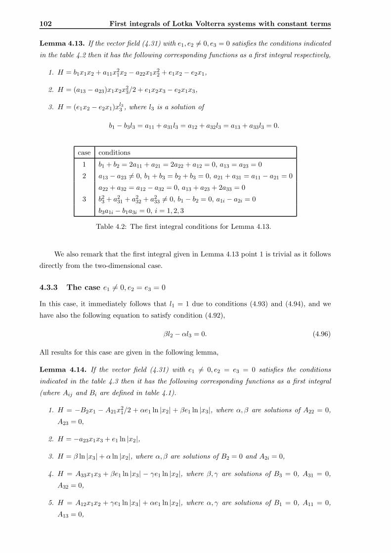
102 First integrals of Lotka Volterra systems with constant terms
Lemma 4.13. If the vector field (4.31) with e1, e2 6= 0, e3 = 0 satisfies the conditions indicated
in the table 4.2 then it has the following corresponding functions as a first integral respectively,
1. H = b1x1x2 + a11x21x2 − a22x1x
22 + e1x2 − e2x1,
2. H = (a13 − a23)x1x2x23/2 + e1x2x3 − e2x1x3,
3. H = (e1x2 − e2x1)xl33 , where l3 is a solution of
b1 − b3l3 = a11 + a31l3 = a12 + a32l3 = a13 + a33l3 = 0.
case conditions
1 b1 + b2 = 2a11 + a21 = 2a22 + a12 = 0, a13 = a23 = 0
2 a13 − a23 6= 0, b1 + b3 = b2 + b3 = 0, a21 + a31 = a11 − a21 = 0
a22 + a32 = a12 − a32 = 0, a13 + a23 + 2a33 = 0
3 b23 + a231 + a2
32 + a233 6= 0, b1 − b2 = 0, a1i − a2i = 0
b3a1i − b1a3i = 0, i = 1, 2, 3
Table 4.2: The first integral conditions for Lemma 4.13.
We also remark that the first integral given in Lemma 4.13 point 1 is trivial as it follows
directly from the two-dimensional case.
4.3.3 The case e1 6= 0, e2 = e3 = 0
In this case, it immediately follows that l1 = 1 due to conditions (4.93) and (4.94), and we
have also the following equation to satisfy condition (4.92),
βl2 − αl3 = 0. (4.96)
All results for this case are given in the following lemma,
Lemma 4.14. If the vector field (4.31) with e1 6= 0, e2 = e3 = 0 satisfies the conditions
indicated in the table 4.3 then it has the following corresponding functions as a first integral
(where Aij and Bi are defined in table 4.1).
1. H = −B2x1 − A21x21/2 + αe1 ln |x2| + βe1 ln |x3|, where α, β are solutions of A22 = 0,
A23 = 0,
2. H = −a23x1x3 + e1 ln |x2|,
3. H = β ln |x3| + α ln |x2|, where α, β are solutions of B2 = 0 and A2i = 0,
4. H = A33x1x3 + βe1 ln |x3| − γe1 ln |x2|, where β, γ are solutions of B3 = 0, A31 = 0,
A32 = 0,
5. H = A12x1x2 + γe1 ln |x3| + αe1 ln |x2|, where α, γ are solutions of B1 = 0, A11 = 0,
A13 = 0,
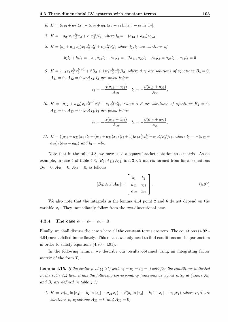
4.3 Three-dimensional LV systems with constant terms 103
6. H = (a13 + a23)x3 − (a12 + a32)x2 + e1 ln |x3| − e1 ln |x2|,
7. H = −a23x1xl22 x3 + e1x
l22 /l2, where l2 = −(a13 + a33)/a23,
8. H = (b1 + a11x1)x1xl22 x
l33 + e1x
l22 x
l33 , where l2, l3 are solutions of
b2l2 + b3l3 = −b1, a21l2 + a31l3 = −2a11, a22l2 + a32l3 = a23l2 + a33l3 = 0
9. H = A33x1xl22 x
l3+13 + β(l3 + 1)e1x
l22 x
l33 /l3, where β, γ are solutions of equations B3 = 0,
A31 = 0, A32 = 0 and l2, l3 are given below
l2 = −α(a13 + a33)
A33l3 = −β(a13 + a33)
A33,
10. H = (a12 + a22)x1xl2+12 xl3
3 + e1xl22 x
l33 , where α, β are solutions of equations B2 = 0,
A21 = 0, A23 = 0 and l2, l3 are given below
l2 = −α(a12 + a22)
A22l3 = −β(a12 + a22)
A22,
11. H = ((a12 +a22)x2/l3 + (a13 +a23)x3/(l3 + 1))x1xl22 x
l33 + e1x
l22 x
l33 /l3, where l2 = −(a12 +
a22)/(a22 − a32) and l3 = −l2.
Note that in the table 4.3, we have used a square bracket notation to a matrix. As an
example, in case 4 of table 4.3, [B3;A31;A32] is a 3 × 2 matrix formed from linear equations
B3 = 0, A31 = 0, A32 = 0, as follows
[B3;A31;A32] =
b1 b2
a11 a21
a12 a22
. (4.97)
We also note that the integrals in the lemma 4.14 point 2 and 6 do not depend on the
variable x1. They immediately follow from the two-dimensional case.
4.3.4 The case e1 = e2 = e3 = 0
Finally, we shall discuss the case where all the constant terms are zero. The equations (4.92 -
4.94) are satisfied immediately. This means we only need to find conditions on the parameters
in order to satisfy equations (4.80 - 4.91).
In the following lemma, we describe our results obtained using an integrating factor
matrix of the form T2.
Lemma 4.15. If the vector field (4.31) with e1 = e2 = e3 = 0 satisfies the conditions indicated
in the table 4.4 then it has the following corresponding functions as a first integral (where Aij
and Bi are defined in table 4.1),
1. H = α(b1 ln |x2| − b2 ln |x1| − a21x1) + β(b1 ln |x3| − b3 ln |x1| − a31x1) where α, β are
solutions of equations A22 = 0 and A23 = 0,
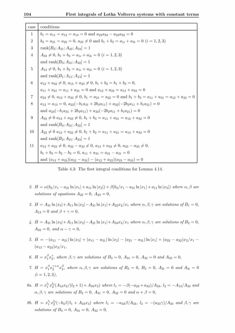
104 First integrals of Lotka Volterra systems with constant terms
case conditions
1 b1 = a11 = a12 = a13 = 0 and a22a33 − a23a32 = 0
2 b2 = a21 = a22 = 0, a23 6= 0 and b1 + b3 = a1i + a3i = 0 (i = 1, 2, 3)
3 rank[B2;A21;A22;A23] = 1
4 A33 6= 0, b1 + b3 = a1i + a3i = 0 (i = 1, 2, 3)
and rank[B3;A31;A32] = 1
5 A12 6= 0, b1 + b2 = a1i + a2i = 0 (i = 1, 2, 3)
and rank[B1;A11;A13] = 1
6 a12 + a32 6= 0, a13 + a23 6= 0, b1 + b2 = b1 + b3 = 0,
a11 + a21 = a11 + a31 = 0 and a12 + a22 = a13 + a33 = 0
7 a23 6= 0, a13 + a33 6= 0, b1 = a21 = a22 = 0 and b1 + b3 = a11 + a31 = a12 + a32 = 0
8 a12 = a13 = 0, a22(−b1a31 + 2b3a11) + a32(−2b2a11 + b1a21) = 0
and a23(−b1a31 + 2b3a11) + a33(−2b2a11 + b1a21) = 0
9 A33 6= 0 a13 + a33 6= 0, b1 + b3 = a11 + a31 = a12 + a32 = 0
and rank[B3;A31;A32] = 1
10 A22 6= 0 a12 + a22 6= 0, b1 + b2 = a11 + a21 = a13 + a33 = 0
and rank[B2;A21;A23] = 1
11 a12 + a22 6= 0, a22 − a32 6= 0, a13 + a33 6= 0, a23 − a33 6= 0,
b1 + b3 = b2 − b3 = 0, a11 + a31 = a21 − a31 = 0
and (a13 + a33)(a22 − a32) − (a12 + a22)(a23 − a33) = 0
Table 4.3: The first integral conditions for Lemma 4.14.
2. H = α(b2/x1 − a21 ln |x1|+ a11 ln |x2|) +β(b3/x1 − a31 ln |x1|+ a11 ln |x3|) where α, β are
solutions of equations A22 = 0, A23 = 0,
3. H = A31 ln |x3|+A11 ln |x2|−A21 ln |x1|+A22x2/x1 where α, β, γ are solutions of B1 = 0,
A13 = 0 and β + γ = 0,
4. H = A31 ln |x3|+A11 ln |x2|−A21 ln |x1|+A33x3/x1 where α, β, γ are solutions of B2 = 0,
A22 = 0, and α− γ = 0,
5. H = −(a11 − a21) ln |x3| + (a11 − a31) ln |x2| − (a21 − a31) ln |x1| + (a22 − a32)x2/x1 −(a13 − a23)x3/x1,
6. H = xβ1x
γ2 , where β, γ are solutions of B3 = 0, A31 = 0, A32 = 0 and A33 = 0,
7. H = xβ1x
γ+α2 xβ
3 , where α, β, γ are solutions of B2 = 0, B3 = 0, A2i = 0 and A3i = 0
(i = 1, 2, 3),
8a. H = xl11 x
l22 (A12x2/(l2 + 1) +A33x3) where l1 = −β(−a23 +a33)/A33, l2 = −A13/A33 and
α, β, γ are solutions of B3 = 0, A31 = 0, A32 = 0 and α+ β = 0,
8b. H = xl11 x
l22 (−b3β/l1 + A33x3) where l1 = −a33β/A33, l2 = −(a33γ)/A33 and β, γ are
solutions of B3 = 0, A31 = 0, A32 = 0,
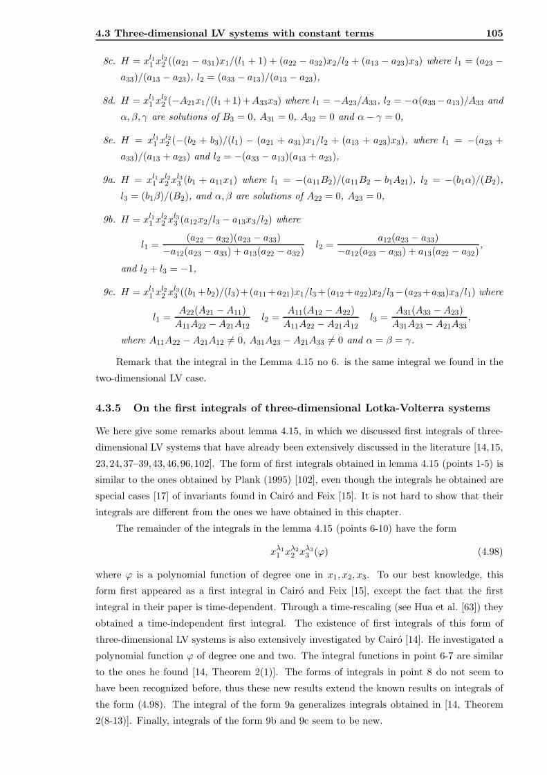
4.3 Three-dimensional LV systems with constant terms 105
8c. H = xl11 x
l22 ((a21 − a31)x1/(l1 + 1) + (a22 − a32)x2/l2 + (a13 − a23)x3) where l1 = (a23 −
a33)/(a13 − a23), l2 = (a33 − a13)/(a13 − a23),
8d. H = xl11 x
l22 (−A21x1/(l1 + 1) +A33x3) where l1 = −A23/A33, l2 = −α(a33−a13)/A33 and
α, β, γ are solutions of B3 = 0, A31 = 0, A32 = 0 and α− γ = 0,
8e. H = xl11 x
l22 (−(b2 + b3)/(l1) − (a21 + a31)x1/l2 + (a13 + a23)x3), where l1 = −(a23 +
a33)/(a13 + a23) and l2 = −(a33 − a13)(a13 + a23),
9a. H = xl11 x
l22 x
l33 (b1 + a11x1) where l1 = −(a11B2)/(a11B2 − b1A21), l2 = −(b1α)/(B2),
l3 = (b1β)/(B2), and α, β are solutions of A22 = 0, A23 = 0,
9b. H = xl11 x
l22 x
l33 (a12x2/l3 − a13x3/l2) where
l1 =(a22 − a32)(a23 − a33)
−a12(a23 − a33) + a13(a22 − a32)l2 =
a12(a23 − a33)
−a12(a23 − a33) + a13(a22 − a32),
and l2 + l3 = −1,
9c. H = xl11 x
l22 x
l33 ((b1 +b2)/(l3)+(a11 +a21)x1/l3 +(a12 +a22)x2/l3−(a23 +a33)x3/l1) where
l1 =A22(A21 −A11)
A11A22 −A21A12l2 =
A11(A12 −A22)
A11A22 −A21A12l3 =
A31(A33 −A23)
A31A23 −A21A33,
where A11A22 −A21A12 6= 0, A31A23 −A21A33 6= 0 and α = β = γ.
Remark that the integral in the Lemma 4.15 no 6. is the same integral we found in the
two-dimensional LV case.
4.3.5 On the first integrals of three-dimensional Lotka-Volterra systems
We here give some remarks about lemma 4.15, in which we discussed first integrals of three-
dimensional LV systems that have already been extensively discussed in the literature [14,15,
23,24,37–39,43,46,96,102]. The form of first integrals obtained in lemma 4.15 (points 1-5) is
similar to the ones obtained by Plank (1995) [102], even though the integrals he obtained are
special cases [17] of invariants found in Cairo and Feix [15]. It is not hard to show that their
integrals are different from the ones we have obtained in this chapter.
The remainder of the integrals in the lemma 4.15 (points 6-10) have the form
xλ1
1 xλ2
2 xλ3
3 (ϕ) (4.98)
where ϕ is a polynomial function of degree one in x1, x2, x3. To our best knowledge, this
form first appeared as a first integral in Cairo and Feix [15], except the fact that the first
integral in their paper is time-dependent. Through a time-rescaling (see Hua et al. [63]) they
obtained a time-independent first integral. The existence of first integrals of this form of
three-dimensional LV systems is also extensively investigated by Cairo [14]. He investigated a
polynomial function ϕ of degree one and two. The integral functions in point 6-7 are similar
to the ones he found [14, Theorem 2(1)]. The forms of integrals in point 8 do not seem to
have been recognized before, thus these new results extend the known results on integrals of
the form (4.98). The integral of the form 9a generalizes integrals obtained in [14, Theorem
2(8-13)]. Finally, integrals of the form 9b and 9c seem to be new.
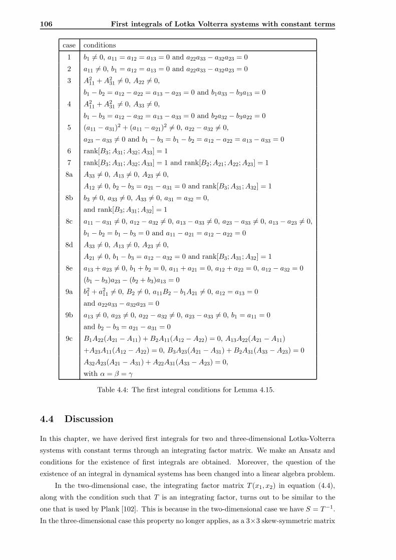
106 First integrals of Lotka Volterra systems with constant terms
case conditions
1 b1 6= 0, a11 = a12 = a13 = 0 and a22a33 − a32a23 = 0
2 a11 6= 0, b1 = a12 = a13 = 0 and a22a33 − a32a23 = 0
3 A211 +A2
31 6= 0, A22 6= 0,
b1 − b2 = a12 − a22 = a13 − a23 = 0 and b1a33 − b3a13 = 0
4 A211 +A2
31 6= 0, A33 6= 0,
b1 − b3 = a12 − a32 = a13 − a33 = 0 and b2a32 − b3a22 = 0
5 (a11 − a31)2 + (a11 − a21)2 6= 0, a22 − a32 6= 0,
a23 − a33 6= 0 and b1 − b3 = b1 − b2 = a12 − a22 = a13 − a33 = 0
6 rank[B3;A31;A32;A33] = 1
7 rank[B3;A31;A32;A33] = 1 and rank[B2;A21;A22;A23] = 1
8a A33 6= 0, A13 6= 0, A23 6= 0,
A12 6= 0, b2 − b3 = a21 − a31 = 0 and rank[B3;A31;A32] = 1
8b b3 6= 0, a33 6= 0, A33 6= 0, a31 = a32 = 0,
and rank[B3;A31;A32] = 1
8c a11 − a31 6= 0, a12 − a32 6= 0, a13 − a33 6= 0, a23 − a33 6= 0, a13 − a23 6= 0,
b1 − b2 = b1 − b3 = 0 and a11 − a21 = a12 − a22 = 0
8d A33 6= 0, A13 6= 0, A23 6= 0,
A21 6= 0, b1 − b3 = a12 − a32 = 0 and rank[B3;A31;A32] = 1
8e a13 + a23 6= 0, b1 + b2 = 0, a11 + a21 = 0, a12 + a22 = 0, a12 − a32 = 0
(b1 − b3)a23 − (b2 + b3)a13 = 0
9a b21 + a211 6= 0, B2 6= 0, a11B2 − b1A21 6= 0, a12 = a13 = 0
and a22a33 − a32a23 = 0
9b a13 6= 0, a23 6= 0, a22 − a32 6= 0, a23 − a33 6= 0, b1 = a11 = 0
and b2 − b3 = a21 − a31 = 0
9c B1A22(A21 −A11) +B2A11(A12 −A22) = 0, A13A22(A21 −A11)
+A23A11(A12 −A22) = 0, B3A23(A21 −A31) +B2A31(A33 −A23) = 0
A32A23(A21 −A31) +A22A31(A33 −A23) = 0,
with α = β = γ
Table 4.4: The first integral conditions for Lemma 4.15.
4.4 Discussion
In this chapter, we have derived first integrals for two and three-dimensional Lotka-Volterra
systems with constant terms through an integrating factor matrix. We make an Ansatz and
conditions for the existence of first integrals are obtained. Moreover, the question of the
existence of an integral in dynamical systems has been changed into a linear algebra problem.
In the two-dimensional case, the integrating factor matrix T (x1, x2) in equation (4.4),
along with the condition such that T is an integrating factor, turns out to be similar to the
one that is used by Plank [102]. This is because in the two-dimensional case we have S = T−1.
In the three-dimensional case this property no longer applies, as a 3×3 skew-symmetric matrix
4.4 Discussion 107
is not invertible. Hence, our analysis is more general than Plank’s, as we did not assume that
there is an isolated equilibrium, as was assumed in his paper.
Comparison with Darboux method The Darboux method has been applied to find first
integrals of two-dimensional [20, 22] and three-dimensional [14, 23] LV systems. Compared
to this method, our method has advantages in the context of searching for a first integral of
Lotka-Volterra systems with constant terms. To apply the Darboux method, one must seek
an algebraic curve of a vector field, and Lotka-Volterra systems without constant terms have
a natural algebraic curve as the systems have invariant axis. For systems with constant terms,
this no longer applies, as the presence of the constant terms make the invariant axis vanish.
Comparison with Hamiltonian method The existence of first integrals of two-dimensional
systems has been obtained using Hamiltonian method [16, 19, 63]. They assumed that the
integrals are products of two or three polynomial functions of degree one. Thus, our method
has advantages in terms of the number of Ansatzs, as we only assume one form of Ansatz.
Gao [37] has also applied a Hamiltonian method to find first and second integrals of special
cases of three-dimensional LV systems, where the linear terms are absent.
Comparison with Frobenius method The Frobenius method was first introduced by Strel-
cyn and Wojciechowski [115] to find a first integral for three-dimensional systems. It has been
used to find integrals for LV systems by Grammaticos et al. [46]. Unfortunately, they only
look at a special case of the LV system, which is the so-called ABC system.
Comparison with Carleman embedding method The existence of first integrals in n
dimensions has been studied [15,18] through the Carleman embedding method. However, the
integrals that are obtained are time-dependent, which is sometimes called an invariant.
For future work, it would be a challenging problem to find a more general integrating
factor matrix of a vector field in dimension greater than or equal to two. People have obtained
first integrals and conditions for the existence of such integrals and we could use their results
to endeavour to find the general integrating factor matrix.

CHAPTER 5
Conclusion
In this final chapter, a summary of all results presented in this thesis is discussed. The
discussion focuses on different aspects of all our analyses of the Lotka-Volterra system with
constant terms. First we focus on the bifurcation analysis that we have done in the chapters
two and three of this thesis. We shall discuss the non-versal unfolding aspect of unusual
bifurcations that we have found in the two-dimensional Lotka-Volterra system with a constant
term in chapter two. We also discuss the idea of bifurcation analysis of systems with a special
structure. The discussion then turns to the issue of the existence of first integrals of two- and
three-dimensional Lotka-Volterra systems with constant terms.
5.1 Bifurcation analysis of Lotka-Volterra systems with a con-
stant term
In chapter two, we have performed bifurcation analysis of the two-dimensional Lotka-Volterra
system with a constant term. In the model (2.1), there are seven parameters available but we
have three continuous symmetries which are used to reduce the number of parameters to be
varied from seven to four. However, we only vary two when performing bifurcation analysis,
as the other two are used to distinguish the topological difference of bifurcation diagrams.
The bifurcation diagrams are very useful in classifying the dynamics of the system we analyse
in terms of parameters that we vary. The bifurcation curves in the bifurcation diagram are
boundaries of different dynamics that can occur. We then can interpret the dynamics in each
area of each bifurcation diagram in terms of the original problem.
We have performed not only bifurcation analysis but also investigated how degenerate our
bifurcations are. In particular, we are interested in bifurcations where saddle-node and trans-
critical bifurcations interact. It turns out that these unusual bifurcations can be considered as
non-versal unfoldings of common bifurcations in general systems which are a codimension-two
cusp bifurcation and a codimension-three degenerate Bogdanov-Takens bifurcation. The cusp
bifurcation has been known for a long time. Since the normal form of a cusp bifurcation is
one-dimensional, the degeneracy of cusp bifurcation naturally appears when varying param-
eters. The cusp bifurcation is one of seven elementary catastrophes listed by Thom [118]
110 Conclusion
along with the simple saddle-node bifurcation. In contrast, a codimension-three degenerate
Bogdanov-Takens bifurcation is still a new theory and rarely occurs in application.
The study of the degenerate Bogdanov-Takens bifurcation is interesting on its own.
Kuznetsov [79] has derived a practical computation to find the coefficient of the normal form of
the Bogdanov-Takens bifurcation. Therefore, we can detect if a Bogdanov-Takens bifurcation
is degenerate and how degenerate it is. Although the global analysis of such a bifurcation is
extensively investigated in Dumortier et al. [31], and all references therein, the occurrence of
this bifurcation is rarely found in applications. To our best knowledge, Baer et al. [6] is one of
the first to find such a bifurcation in an application, i.e. in a model for a two-stage structured
population.
Our approach to understand unusual bifurcations that we have found is to prove that
these bifurcations are actually non-versal unfoldings of common bifurcations such as cusp and
Bogdanov-Takens bifurcations. We have introduced minimal models that undergo the same
bifurcations as we have. We also have tried to find non-linear smooth maps that respectively
transform our model to the minimal model and transform the minimal model to the normal
form of a generic bifurcation that is already known. However, in this chapter we did not answer
the question of why, in the first place, our model has such unusual bifurcations. This question
has been answered in the next chapter where we discuss systems with a special structure.
5.2 Dynamical systems with a special structure
In chapter three we have discussed dynamical systems with a codimension-one invariant man-
ifold. We have applied bifurcation analysis to those systems, imposing that the analysis
preserves the property of the special structure. We started with the simplest degeneracy that
a system can have which is the single-zero eigenvalue. It turns out that we have a transcritical
bifurcation instead of a more generic saddle-node bifurcation. Another consequence of the
codimension-one invariant manifold in the codimension-one degeneracy is the fact that we
cannot have a Hopf bifurcation.
Continuing to higher codimension bifurcations (i.e. codimension-two bifurcations), we
have analysed more degenerate singularities that are similar to cusp, Bogdanov-Takens and
fold-Hopf bifurcations respectively. The degeneracies that we have discussed are similar to
those generic codimension-two bifurcations, but give us different sets of bifurcations as a result
of the special structure that our system has, which is a codimension-one invariant manifold.
In the first case, the cusp bifurcation is unfolded in a different way such that we have found
an interaction of saddle-node and transcritical bifurcations. However, in the double-zero
degeneracy, the Bogdanov-Takens bifurcation is not unfolded differently, instead we come to
a more degenerate codimension-three Bogdanov-Takens bifurcation. This can be checked by
computing the normal form coefficients of this bifurcation.
We now want to discuss the connection between the bifurcation analysis of dynamical sys-
tems with a special structure and the two-dimensional Lotka-Volterra system with a constant
term. The bifurcation structure of the Lotka-Volterra system contains two important degen-
5.3 The existence of first integrals of LV systems with constant terms 111
erate bifurcations that we have studied in this thesis in chapter two, namely the single-zero
eigenvalue degeneracy combined with second order degeneracy and the double-zero eigenvalue
degeneracy. Both of these degeneracies are shown in chapter three to produce the same set of
bifurcations as the Lotka-Volterra system does. Therefore, the Lotka-Volterra system with a
constant term has such unusual bifurcations mainly because it has a codimension-one invariant
manifold structure.
Thus, we have two approaches in explaining bifurcations in the Lotka-Volterra system.
One is to understand generic bifurcations and to try to relate them to bifurcations in our
system. The other approach is to understand the special structure that our system has, in
this case the special structure is the invariant manifold. Between these two approaches, the
latter seems more common as the analysis of a special structure has its own place in dynamical
system theory. For example, the study of dynamical system with a special structure which is
a symmetry has been studied in great detail [82].
Another special structure that may be pursued in future work is a codimension-two
invariant manifold in our system. The manifold that is discussed in this thesis is one dimension
less than the space we are working with, thus there are some bifurcations that are just not
allowed to occur such as the Hopf bifurcation as a codimension-one bifurcation, a degenerate
Hopf, and a double-Hopf bifurcations as codimension-two bifurcations. If we can reduce
the dimension of the invariant manifold, we shall have more exciting bifurcations as more
bifurcations are allowed.
5.3 The existence of first integrals of Lotka-Volterra systems
with constant terms
The existence of first integrals of Lotka-Volterra systems with constant terms has been dis-
cussed in chapter four. Various authors have obtained first integrals and conditions on the
parameters for the Lotka-Volterra system without the constant terms, while we have found
first integrals and conditions on the parameters for the Lotka-Volterra system including ad-
ditional constant terms. The integrating factor matrix method has been used to reduce the
problem of searching for a first integral to a linear algebra problem. We want to mention
that the conditions for the Lotka-Volterra system with constant terms do not depend on the
constant terms. As a consequence, the model has a first integral for all values of the constant
terms.
The question that we then want to discuss is what the first integral function and its
constraint are used for. As mentioned in the beginning of the chapter four, finding first
integrals is a classical tool in the classification of phase portraits of a dynamical system. Not
only that but finding first integrals gives global information about the long-term behaviour
of dynamical systems. Another reason why the existence of such a function is studied, is
to find the location of global bifurcations in the parameter space. This analysis is actually
discussed in chapter three. The Melnikov method that is applied to a differential equation,
needs a reduced integrable model of the same differential equation as a starting point for
112 Conclusion
a perturbation method in finding the location of heteroclinic or homoclinic bifurcations. It
is true that recently, the detection of global bifurcation has used a numerical continuation
package like AUTO2000 (see Doedel et al. [29]). However, it is always nice to compute the
formula for global bifurcations analytically.
Another reason why first integrals of differential equations are important is because the
first integral is used in the theory of numerical methods to solve differential equations, in
particular in geometrical integration. We refer to Quispel and McLachlan [104] for a more
detailed explanation of the theory of geometrical integration. Geometric integration is the
term used to describe numerical methods for computing the solution of differential equations,
while preserving one or more physical/mathematical properties of the system exactly (i.e. up
to roundoff error). If a dynamical system has a first integral, then the integral can be used
in test equations for geometrical numerical integration methods. For instance, we refer to
Nakamura and Hashimoto [99] in which a comparison is made between geometrical numerical
integration schemes applied to three-dimensional Lotka-Volterra systems.
In the discussion of chapter four, we have compared our methods with known methods
to find first integrals such as the Carleman embedding method, the Frobenius method, the
Darboux method and the Hamiltonian method. Each of these methods obtained a first integral
along with its conditions on the parameters. Using their results, it would be a challenging
problem to find a more general integrating factor matrix of a vector field in dimension greater
than or equal to two.
We also remark that searching for a first integral does not always give a completely
integrable case. It is true that in two-dimensional systems, the existence of a first integral
implies that the system is completely integrable because the phase portraits are completely
characterized. However, in three-dimensional systems (or greater than three) this is not the
case. Thus, there is still a problem to find a second integral. Note that the existence of a
second integral gives a completely integrable case in three-dimensional vector fields.
In the end, to prove the integrability or to prove the existence of integrals of general
differential equations is very hard and no systematic methods to solve it are known. All
attempts described above do not completely solve this integrability problem but represent
approaches in this direction.
5.4 Final words
After almost a century, the Lotka-Volterra model is still intriguing many mathematicians.
This model has been used to approximate many applications in the real world and thus there
have been a large number of modifications to this model such that the physical problem can be
approximated as closely as possible. In addition to real world applications, this model is also
interesting from a mathematical point of view, as many aspects and theories in mathematics
have been applied to understand the behaviour of the solution of this model. The conditions
for this system to be integrable and the bifurcation analysis of this system that have been
introduced in this thesis are just some of a number of mathematical investigations on this
model around the world.
5.4 Final words 113
Dynamical systems theory, which has provided tools to analyse such systems in this thesis,
is interesting in its own right. This theory has seen an explosive growth and expansion in the
past 50 years. Integrability and bifurcation analysis are among methods of global analysis in
dynamical systems theory. Finally, we cannot restrict ourselves to dynamical systems theory
to analyse such system, as the Lotka-Volterra system has also attracted much attention in
other branches of mathematics.

APPENDIX A
Proof of Proposition (3.6)
We recall the proposition (3.6),
The center manifold of a single-zero eigenvalue or a pair of purely imaginary eigenvalue of
the matrix (3.4) lies inside the codimension-one invariant manifold up to any desired degree
of accuracy.
We shall prove this proposition. First we shall consider the case when the matrix (3.4) has a
single zero eigenvalue. We already assumed that the origin is an equilibrium. We recall the
equation (3.2),
x1 = f1(x1, x2, . . . , xn−1, y),
x2 = f2(x1, x2, . . . , xn−1, y),...
xn−1 = fn−1(x1, x2, . . . , xn−1, y),
y = yfn(x1, x2, . . . , xn−1, y).
Without loss of generality, we assume that the Jacobian matrix of the equation above evaluated
at the origin has been transformed into a (real) Jordan canonical form. Suppose that the single-
zero eigenvalue occurs in the x1-direction, then by the center manifold theorem applied to the
coordinates (x1, . . . , xn−1), we can assume that the vector field is two-dimensional. Thus, we
havex1 = f1(x1, y),
y = yf2(x1, y),(A.1)
where f1 is nonlinear in x1 and y. By using the center manifold theorem, there is a function
y = h(x1) such that the dynamics restricted to the center manifold is given by,
x1 = f1(x1, h(x1)).
We want to prove that the center manifold lies entirely inside the codimension-one invariant
manifold y = 0, thus we need to show h(x1) = 0. We assume h(x1) has the form,
h(x1) = h2x21 + h3x
31 + h4x
41 + . . . .
We Taylor expand the functions f1(x1, y) and f2(x1, y),
f1(x1, y) = f(20)1 x2
1 + f(11)1 x1y + f
(02)1 y2 + . . . ,
f2(x1, y) = f(00)2 + f
(10)2 x1 + f
(01)2 y + . . . ,
116 Proof of Proposition (3.6)
where f(00)2 6= 0 since the Jacobian matrix of the system (A.1) has only a single-zero eigenvalue.
We finally compute the derivative of y = h(x1) with respect to time,
y = dhdx1
x1,
yf2(x1, y) = (2h2x1 + 3h3x21 + 4h4x
31 + . . .)f1(x1, y),
h(x1)f2(x1, h(x1)) = (2h2x1 + 3h3x21 + 4h4x
31 + . . .)f1(x1, h(x1)).
Using the Taylor expansion of the functions f1(x1, y) and f2(x1, y), we can compute the
coefficients of the function h(x1) by equating coefficients of x1 that have the same power. The
smallest power of x1 in the left hand side is two, while that of the right hand side is three.
This gives h2 = 0. The fact that h2 = 0 implies that the smallest power of x1 in the left hand
side is three, while that of the right hand side is now four. This now gives h3 = 0. It will
continue this way, in fact, we will get hi = 0 for i = 2, 3, . . .. This implies that the center
manifold is y = 0, which is the same equation as the invariant manifold. Thus, the first part
of the proposition is proven.
We now want to prove the second part which is to show that the center manifold coming
from a pair of purely imaginary eigenvalue degeneracy also lies inside the invariant manifold
up to any desired degree of accuracy. However, we shall only prove that the center manifold
lies inside the invariant manifold up the third order term.
Without loss of generality, we assume that the Jacobian matrix evaluated at the origin
has been transformed into a (real) Jordan canonical form. By using the center manifold
theorem applied to the coordinate (x1, . . . , xn−1), we can assume that the vector field is three-
dimensional. Thus, we have
x1 = −x2 + f1(x1, x2, y),
x2 = x1 + f2(x1, x2, y),
y = yf3(x1, x2, y),
where f1,f2 are nonlinear in x1,x2 and y and f3(0, 0, 0) is not zero. By the center manifold
theorem, there is a function y = h(x1, x2). We want to prove that h(x1, x2) = 0. First we
assume that h(x1, x2) has the following form,
h(x1) = h20x21 + h11x1x2 + h02x
22 + . . . .
Computing the derivative of y = h(x1, x2) with respect to time gives,
y = ∂h∂x1
x1 + ∂h∂x2
x2,
yf3(x1, x2, y) = ∂h∂x1
(−x2 + f1(x1, x2, y)) + ∂h∂x2
(x1 + f2(x1, x2, y)),
h(x1, x2)f3(x1, x2, h(x1, x2)) = ∂h∂x1
(−x2 + f1(x1, x2, h(x1, x2))) + ∂h∂x2
(x1 + f2(x1, x2, h(x1, x2))).
By Taylor expanding the functions f1(x1, x2, y), f2(x1, x2, y), and f3(x1, x2, y), we are able to
compute the coefficient of the function h(x1, x2) by equating coefficients that have the same
power in terms of x1 and x2. Equating the second order terms gives,
(x21) : h20f3(0, 0, 0) = h11,
(x1x2) : h11f3(0, 0, 0) = −2h20 + 2h02,
(x22) : h02f3(0, 0, 0) = −h11.
117
The only solution of the linear system above is (h20, h11, h02) = (0, 0, 0), which is what we
want. We then compute the coefficients of third order,
(x31) : h30f3(0, 0, 0) = h21,
(x21x2) : h21f3(0, 0, 0) = −3h30 + 2h12,
(x1x22) : h12f3(0, 0, 0) = −2h21 + 3h03,
(x32) : h03f3(0, 0, 0) = −h12,
which gives trivial solutions (h30, h21, h12, h02) = (0, 0, 0, 0). Thus, we have proven that the
center manifold coming from a pair of purely imaginary eigenvalue degeneracy lies inside the
invariant manifold up to the third order term.

APPENDIX B
Bifurcation analysis of theLotka-Volterra system with a
constant term
In this appendix, we shall check conditions of bifurcations that occur in the Lotka-Volterra
system with a constant term (2.1). As depicted in Figure 2.1, numerous bifurcations occur in
this system. The conditions for saddle-node and transcritical bifurcations that are obtained
analytically are going to be discussed in this appendix.
B.1 Bifurcation conditions of the first saddle-node bifurcation
We first check conditions for the first saddle-node bifurcation to occur. The saddle-node
bifurcation occurs when the coordinates and the parameters are:
x∗1 = − b12a11
, e∗ =b21
4a211
,
x∗2 = 0,
(B.1)
where a11 6= 0. Along the line e = b21/(4a211), the Jacobian matrix of the system (2.1) evaluated
at this equilibrium has two eigenvalues, which are
λ1 = 0 and λ2 = b2 −b1a21
2a11.
We assume that λ2 = b2 − b1a21/(2a11) 6= 0, since the only degeneracy is a single-zero eigen-
value. We translate the critical equilibrium to the origin and consider e as one of the coordi-
nates by introducing a new coordinate system, y1 = x1 − x∗1, y2 = x2 − x∗2 and y3 = e − e∗,
thus we have
y1 = γy2 + y3 + a11y21 + a12y1y2,
y2 = (b2 −b1a21
2a11)y2 + a21y1y2 + a22y
22, (B.2)
y3 = 0,
where γ = −b1a12/(2a11). To check the saddle-node bifurcation conditions we need to first
diagonalize the system above and to apply the center manifold theorem to reduce the diago-
120 Bifurcation analysis of the Lotka-Volterra system with a constant term
nalized system restricted to the center manifold. A transformation given by
y1
y2
y3
=
1 2a11γ 0
0 2b2a11 − b1a21 0
0 0 1
u1
u2
α
, (B.3)
will bring the system (B.2) to the following diagonalized system,
u1 = α+ a11u21 + C1u1u2 + C2u
22,
u2 = (b2 −b1a21
2a11)u2 + a21u1u2 + C3u
22, (B.4)
α = 0,
where
C1 = −2a11a21γ + a21(2b2a11 − b1a21)4a211γ,
C2 = 2a11γ(2a211γ − 2a21a11γ − a22(2b2a11 − b1a21) + a12(2b2a11 − b1a21)),
C3 = (2a11a21γ + (2b2a11 − b1a21)a22).
By using the center manifold theorem, there is a function u2 = h(u1, α) ∈ O(‖(u1, α)‖2) for
a sufficiently small neighbourhood (u1, α) = (0, 0) such that the dynamics restricted to the
center manifold is represented by,
u1 = f(α, u1) = α+ a11u21 + C1u1h(u1, α) + C2h(u1, α)2. (B.5)
The degeneracy condition for saddle-node bifurcation is,
∂f
∂u1(0, 0) = 0, (B.6)
while the non-degeneracy conditions are
∂f
∂α(0, 0) = 1, and
∂2f
∂u21
= 2a11. (B.7)
We conclude that the Lotka-Volterra system with a constant term undergoes a codimension-
one saddle-node bifurcation along the line e = b21/(4a11) with a11 6= 0. However, there
are some values of the parameters such that the bifurcation is degenerate which is when
(b2 − b1a21/(2a11)) = 0, in which we have a double-zero eigenvalues degeneracy.
B.2 Bifurcation conditions of the second saddle-node bifurca-
tion
The second saddle-node bifurcation occurs when
x∗1 = ρ, e∗ =(−b1a22 + b2a12)2
4a22D1,
x∗2 =−b2 − a21ρ
a22,
(B.8)
B.2 Bifurcation conditions of the second saddle-node bifurcation 121
where D1 = a11a22 − a12a21 and ρ = (−b1a22 + b2a12)/(2D1). We assume that D1, a22 6= 0.
Along the line e = (−b1a22 + b2a12)2/(4a22D1), the Jacobian matrix of the system (2.1)
evaluated at this equilibrium has two eigenvalues, which are
λ1 = 0 and λ2 =a12a21ρ− b2a22 − a21a22ρ
a22,
where we assume λ2 is not zero as there is no other degeneracy. After an initial transformation,
given by y1 = x1−x∗1, y2 = x2−x∗2 and y3 = e−e∗, the Lotka-Volterra system with a constant
term can be written as the extended system,
y1 =a12a21
a22y1 + a12ρy2 + y3 + a11y
21 + a12y1y2,
y2 = −a22
a21(b2 + a21ρ)y1 − (b2 + a21ρ)y2 + a21y1y2 + a22y
22,
y3 = 0.
(B.9)
We diagonalize the system above using the following transformation,
y1
y2
y3
=
a22 −a12ρ 0
−a21 (b2 + a21ρ) 0
0 0 1
u1
u2
α
, (B.10)
thus we now have
u1 = α− D1(b2 + a21ρ)
λ2u2
1 −a11a22
λ2(b2 + a21ρ)α2 + p1u1α+ p2u2α+ p3u1u2 + p4u
22,
u2 = λ2u2 −D1a21
λ2u2
1 −a11a22a21
λ2(b2 + a21ρ)2α2 + q1u1α+ q2u2α+ q3u1u2 + q4u
22, (B.11)
α = 0,
where
p1 = −D2
λ2+
a12a221ρ
λ2(b2 + a21ρ), q1 = − a21D3
λ2(b2 + a21ρ),
p2 = −a12
λ2(−(2a11 − a21)ρ+ (b2 + a21ρ)), q2 =
2a11a12a21ρ
λ2(b2 + a21ρ)− a21(a12 + a22)
λ2,
p3 = b2a12 +2a12ρD1(b2 + a21ρ)
a22λ2, q3 =
a21(b2 + a21ρ)(a22 − a12)
λ2+a12a21ρD3
a21λ2,
p4 = −a12ρ(b2 + a21ρ)
a22λ2(a12ρ(a11 − a21) q4 =
1
a22λ2(−a11a21a
212ρ
2 − a222(b2 + a21ρ)2
+ (b2 + a21ρ)(a22 − a12)), + a12a21ρ(b2 + a21ρ)(a12 + a22)),
with D2 = 2a11a22 − a12a21 and D3 = 2a11a22 − a22a21 − a12a21. This system has a two-
dimensional center manifold which can be represented locally as the graph of a polynomial
function u2 = h(u1, α). The function h(u1, α) is assumed to have the following form,
h(u1, α) = h20u21 + h11u1α+ h02α
2 + O(‖(u1, α)‖2). (B.12)
We are not going to compute the coefficient of the polynomial above because we only want
to prove the saddle-node bifurcation conditions. Thus, the dynamics restricted to the center
manifold is represented by the following system,
u1 = f(u1, α)
= α− D1(b2 + a21ρ)
λ2u2
1 −a11a22
λ2(b2 + a21ρ)α2 + p1u1α+ p2αh(u1, α)
+ p3u1h(u1, α) + p4h(u1, α)2. (B.13)
122 Bifurcation analysis of the Lotka-Volterra system with a constant term
The degeneracy condition of this bifurcation is
∂f
∂u1(0, 0) = 0, (B.14)
while the non-degeneracy conditions are
∂f
∂α(0, 0) = 1, and
∂2f
∂u21
= −2D1(b2 + a21ρ)
λ2. (B.15)
We now conclude that the Lotka-Volterra system with a constant term undergoes another
codimension-one saddle-node bifurcation along the line e = (−b1a22 + b2a12)2/(4a22D1) with
a22D1 6= 0. This bifurcation is degenerate when the term (b2 + a21ρ) is zero, in which we
have a degenerate saddle-node bifurcation with a degeneracy in the second order term or
λ2 = (a12a21ρ − b2a22 − a21a22ρ)/a22 is zero in which we have a double-zero eigenvalues
degeneracy.
B.3 Bifurcation conditions of the transcritical bifurcation
The transcritical bifurcation occurs when
x∗1 =b2a21
, e∗ =b2(−b2a11 + b1a21)
a 221
,
x∗2 = 0,
(B.16)
We assume that a21 6= 0. Along the line e = (b2(−b2a11 + b1a21))/a221, the Jacobian matrix of
the system (2.1) evaluated at this equilibrium has two eigenvalues, which are
λ1 = b1 −2b2a11
a21and λ2 = 0.
We assume that λ1 = b1 − (2b2a11)/a21 6= 0 as there is no other degeneracy. We note that this
assumption is equivalent with the assumption that we have in the first saddle-node bifurcation
condition in the appendix B.1. We first transform the critical equilibrium to the origin by the
transformation y1 = x1 − x∗1, y2 = x2 − x∗2 and y3 = e − e∗. We thus have the new extended
vector field as follows
y1 = λ1y1 − (b2a12
a21)y2 + y3 + a11y
21 + a12y1y2
y2 = a21y1y2 + a22y22
y3 = 0. (B.17)
We diagonalize the above vector field by the following linear transformation,
y1
y2
y3
=
1 b2a12 a21
0 (b1a21 − 2b2a11) 0
0 0 −(b1a21 − 2b2a11)
u1
u2
α
, (B.18)
to get the following vector field,
u1 = λ1u1 + a11u21 + (b1 − b2)a12a21u1u2 + (b1 − b2)a12a
221u2u3 + 2a11a21u1u3
+ a11a221u
23 + b2a12(b2D1 + (a22 − a12)(b2a11 − b1a21))u2
2
u2 = a321αu2 + a21u1u2 − 2D1(b2 + a21ρ)u2
2
α = 0, (B.19)
B.3 Bifurcation conditions of the transcritical bifurcation 123
where D1 = a11a22 − a12a21 and ρ = (−b1a22 + b2a12)/(2D1) as in the previous section. The
system above has a two-dimensional center manifold which can be represented locally as the
graph of a polynomial function u1 = h(u2, α). The function h(u2, α) is assumed to have the
form
h(u2, α) = h20u22 + h11u2α+ h02α
2 + O(‖(u2, α)3‖). (B.20)
Thus, the dynamics restricted to the center manifold is represented by the following equation,
u2 = a221αu2 − 2D1(b2 + a21ρ)u2
2 + a21u2h(u2, α). (B.21)
We set the right hand side of the one-dimensional vector field above as f(u2, α) to check the
transcritical bifurcation degeneracy conditions
∂f
∂u2(0, 0) = 0,
∂f
∂α(0, 0) = 0, (B.22)
and the non-degeneracy conditions respectively,
∂2f
∂u2∂α(0, 0) = a2
21,∂2f
∂u22
(0, 0) = −4D1(b2 + a21ρ), (B.23)
since the function h(u2, α) is at least of second order in terms of u2 and α. Therefore we con-
clude that a codimension-one transcritical bifurcation occurs along the line e = (b2(−b2a11 +
b1a21))/a221 with non-zero a21. This bifurcation is degenerate when either of these two following
conditions occur:
1. λ1 = b1 − (2b2a11)/a21 is zero, or
2. (b2 + a21ρ) is zero.
We note that if the first condition holds that we have a degenerate codimension-two bifur-
cation at which the transcritical bifurcation condition coincides with the first saddle-node
bifurcation condition to form a double-zero degeneracy. While, if the second condition holds
the transcritical bifurcation condition coincides with the second saddle-node bifurcation con-
dition to form a codimension-two bifurcation with a single-zero eigenvalue combined with a
degeneracy in the second order term.

APPENDIX C
Degeneracy and non-degeneracyconditions for bifurcations in
Chapter 3
C.1 Bifurcations of the normal form with a double-zero eigen-
values degeneracy
In this section, we will check bifurcation conditions of the saddle-node and the transcritical
bifurcation that occur in the unfolding of the normal form of the double-zero eigenvalues
degeneracy in the system (3.40) in section 3.4.
C.1.1 Bifurcation conditions of the saddle-node bifurcation
First we shall check bifurcation conditions for the codimension-one saddle-node bifurcation
that occurs when
(x, y) = (0, 0) and µ1 = 0. (C.1)
Along the line µ1 = 0, the Jacobian matrix of the system (3.40) has two eigenvalues, which
are
λ1 = 0 and λ2 = µ2. (C.2)
We extend the vector field (3.40) to be three-dimensional by considering the parameter µ1 as
one of the coordinates, thus we have
x = µ1 + y + ax2,
y = y(µ2 + bx),
µ1 = 0.
(C.3)
We diagonalize the system above by the following transformation
x
y
µ1
=
1 1 0
0 µ2 0
0 0 1
u1
u2
α
, (C.4)
126 Degeneracy and non-degeneracy conditions for bifurcations in Chapter 3
to get the following new system
u1 = α+ au21 + (2a− b)u1u2 + (a− b)u2
2,
u2 = µ2u2 + bu1u2 + bu22,
α = 0.
(C.5)
By applying the center manifold theorem, there is a function u2 = h(u1, α) that is of at least
second order such that the dynamics restricted to the center manifold is represented by
u1 = f(u1, α) = α+ au21 + (2a− b)u1u2 + (a− b)u2
2. (C.6)
We do not compute the coefficient of the function u2 = h(u1, α) as the saddle-node bifurcation
condition can be determined without computing this function. The degeneracy condition of
the saddle-node bifurcation is∂f
∂u1(0, 0) = 0, (C.7)
while the non-degeneracy conditions are
∂f
∂α(0, 0) = 1 and
∂2f
∂u21
(0, 0) = 2a. (C.8)
Therefore we conclude that a codimension-one saddle-node bifurcation occurs along the line
µ1 = 0. This bifurcation is degenerate when µ2 = 0 in which we shall have a double-zero
eigenvalue degeneracy.
C.1.2 Bifurcation conditions of the transcritical bifurcation
We shall check the system (3.40) that undergoes a transcritical bifurcation when
(x, y) = (−µ2
b, 0) and µ1 +
a
b2µ2
2 = 0. (C.9)
Along the curve µ1 +a/b2µ22 = 0, the Jacobian matrix of system (3.40) evaluated at this fixed
point has two eigenvalues, which are
λ1 = −2aµ2
band λ2 = 0.
We now translate the critical equilibrium above, also we consider the parameter µ1 as one of
the coordinates,
z1 = x+µ2
b, z2 = y and z3 = µ1 +
a
b2µ2
2.
Thus, we have the new extended vector field as follows,
z1 = −2aµ2
bz1 + z2 + z3 + az2
1 ,
z2 = bz1z2,
z3 = 0.
(C.10)
Again, we diagonalize the system above by the following linear transformation,
z1
z2
z3
=
1 b 0
0 2aµ2 1
0 0 −1
u1
u2
α
. (C.11)
C.2 Bifurcations of the normal form with a single-zero and a pair of purelyimaginary eigenvalues degeneracies 127
Thus we have,
u1 = −2aµ2
bu1 + au2
1 −b2
2aµ2u1α− b3
2aµ2u2α+ b(2a− b)u1u2 + b2(a− b)u2
2,
u2 =b2
2aµ2u2α+ b2u2
2 +b
2aµ2u1α+ bu1u2,
α = 0.
(C.12)
The system above has a two-dimensional center manifold that is represented by a graph of
a polynomial function u1 = h(u2, α) that is of at least second order in terms of u1 and α.
Then the dynamics restricted to the center manifold can be represented by the following
one-dimensional vector field,
u2 = − b2
2aµ2u2α+ b2u2
2 +b
2aµ2αh(u2, α) + bu2h(u2, α). (C.13)
Setting the right hand side of the system above as f(u2, α), we compute the degeneracy
conditions of this bifurcation
∂f
∂u2(0, 0) = 0 and
∂f
∂α(0, 0) = 0,
while the non-degeneracy conditions are given by,
∂2f
∂u22
(0, 0) = 2b2 and∂2f
∂u2∂α(0, 0) =
b2
2aµ2.
Therefore, we conclude that a codimension-one transcritical bifurcation occurs in the unfolding
of the normal form with double-zero eigenvalue degeneracy. This bifurcation is degenerate
when µ2 = 0 at which we have a double-zero eigenvalue degeneracy.
C.2 Bifurcations of the normal form with a single-zero and a
pair of purely imaginary eigenvalues degeneracies
In this section, we check the degeneracy and non-degeneracy conditions of bifurcations in
the unfolding of normal forms with a single-zero and a pair of purely imaginary eigenvalues
(3.84) in section 3.5. There are four bifurcations that we shall check, namely two transcritical
bifurcations and two pitchfork bifurcations.
C.2.1 The first pitchfork bifurcation
The pitchfork bifurcation occurs when
(r, y) = (0, 0) and µ1 = 0
Along the line µ1 = 0, the Jacobian matrix of the system (3.84) has two eigenvalues:
λ1 = 0 and λ2 = µ2.
We extend the system (3.84) by including the parameter µ1 as one of the coordinates,
r = µ1r + a1ry + a2r3,
y = y(µ2 − y − r2). (C.14)
µ1 = 0,
128 Degeneracy and non-degeneracy conditions for bifurcations in Chapter 3
with non-zero µ2, a1 and a2. The system above is already in the diagonal form, thus there
is a two-dimensional center manifold represented by the graph of a polynomial function y =
h(r, µ1). The function y = h(r, µ1) is of at least second order in terms of the coordinate y
and the parameter µ1. The dynamics of the system above restricted to the center manifold is
given by:
r = f(r, µ1) = µ1r + a1rh(r, µ1) + a2r3. (C.15)
We want to compute the degeneracy and non-degeneracy conditions of the pitchfork bifurca-
tion, which include computations of the third derivative of f with respect to r. For this reason
we shall compute the second order coefficients of the center manifold function h(r, µ1). First
we assume that h(r, µ1) has the following form,
y = h(r, µ1) = h20r2 + h11rµ1 + h02µ
21 + . . . . (C.16)
We compute the derivative of both sides of the equation above with respect to time,
y =∂h
∂r(r, µ1)r +
∂h
∂µ1(r, µ1)µ1, (C.17)
µ2y − y2 − r2y = (2h20r + h11µ1 + . . .)(µ1r + a1ry + a2r3) + 0,
µ2h(r, µ1) − h2(r, µ1) − r2h(r, µ1) = (2h20r + h11µ1 + . . .)(µ1r + a1rh(r, µ1) + a2r3).
We equate the coefficients of riµj1 with i + j ≥ 2. However, the smallest power in the right
hand side of the equation above is three, while the smallest power in the left hand side of the
equation above is two. Thus we can conclude that h20 = h11 = h02 = 0. This implies that the
vector field restricted to the center manifold is given by,
r = f(r, µ1) = µ1r + a2r3 + O(‖(r, µ1)‖4).
The degeneracy conditions of the system above are,
∂f
∂r(0, 0) = 0,
∂f
∂µ1(0, 0) = 0 and
∂2f
∂r2(0, 0) = 0,
and the non-degeneracy conditions are
∂2f
∂r∂µ1(0, 0) = 1 and
∂3f
∂r3(0, 0) = 6a2.
Therefore we conclude that a codimension-one pitchfork bifurcation occurs in the system
(3.84). We require that µ2 6= 0 such that this bifurcation is non-degenerate.
C.2.2 The second pitchfork bifurcation
The second pitchfork bifurcation occurs in the system (3.84) when
(r, y) = (0, µ2) and µ1 + a1µ2 = 0.
Along the line µ1 + a1µ2 = 0, the Jacobian matrix of the system (3.84) has two eigenvalues:
λ1 = 0 and λ2 = −µ2.
C.2 Bifurcations of the normal form with a single-zero and a pair of purelyimaginary eigenvalues degeneracies 129
We bring the critical fixed point to the origin and consider µ1 as one of the coordinates, by
using the transformation z1 = r, z2 = y − µ2 and z3 = µ1 + a1µ2. Thus we have
z1 = z1z3 + a1z1z2 + a2z31 ,
z2 = −µ2z2 − µ2z21 − z2
2 − z21z2, (C.18)
z3 = 0.
The system above is already in the diagonal form, then there is a two-dimensional center
manifold represented by a graph of a polynomial function z2 = h(z1, µ1) that is of at least
second order in terms of the coordinate z1 and the parameter z3. Thus the dynamics of the
system above restricted to the center manifold is represented by the following vector field,
z1 = f(z1, z3) = z1z3 + a2z31 + a1z1h(z1, µ1). (C.19)
As in the previous section, one of the non-degeneracy conditions of the pitchfork bifurcation
involves a third derivative of f with respect to z1. Thus we have to compute the coefficients
of the terms zi1z
j3 with i+ j = 2. We assume that the function z2 = h(z1, z3) has the following
form,
h(z1, z3) = h20z21 + h11z1z3 + h02z
23 + . . . ,
and we compute the derivative of z2 = h(z1, z3) with respect to time,
z2 =∂h
∂z1(z1z3)z1 +
∂h
∂z3(z1z3)z3,
−µ2z2 − µ2z21 − z2
2 − z21z2 = (2h20z1 + h11z3 + . . . )(z1z3 + a1z1z2
+ a2z31) + 0,
−µ2h(z1, z3) − µ2z21 − h2(z1, z3) − z2
1h(z1, z3) = (2h20z1 + h11z3 + . . . )(z1z3
+ a1z1h(z1, z3) + a2z31). (C.20)
Equating the coefficient of zi1z
j3 with i+ j = 2 that has the same power on both sides we can
compute the coefficients of the polynomial function h(z1, z2),
(z21) : −µ2h20 − µ2 = 0,
−µ2h20 = µ2,
h20 = −1,
(z1z3) : −µ2h11 = 0,
h11 = 0,
(z23) : −µ2h02 = 0,
h02 = 0.
(C.21)
Thus, the system (C.19) now reads,
z1 = z3z1 + (a2 − a1)z31 + O(‖(z1, z3)‖4). (C.22)
Therefore, the degeneracy conditions of the pitchfork bifurcation are,
∂f
∂z1(0, 0) = 0,
∂f
∂z3(0, 0) = 0 and
∂2f
∂z21
(0, 0) = 0,
130 Degeneracy and non-degeneracy conditions for bifurcations in Chapter 3
while, the non-degeneracy conditions are
∂2f
∂z1∂z3(0, 0) = 1 and
∂3f
∂z31
(0, 0) = 6(a2 − a1).
The term (a2 − a1) is not zero as it has been assumed in the text in section 3.5. We conclude
that a codimension-one pitchfork bifurcation occurs in the system (3.84). This bifurcation is
degenerate when both µ1 and µ2 are zero.
C.2.3 The first transcritical bifurcation
The system (3.84) also undergoes a transcritical bifurcation. The fixed point and the value of
the parameters are
(r, y) = (0, 0) and µ2 = 0.
Along the line µ2 = 0, the Jacobian matrix of the system (3.84) has two eigenvalues:
λ1 = µ1 and λ2 = 0.
We include the parameter µ2 as one of of the coordinates, thus we have:
r = µ1r + a1ry + a2r3,
y = y(µ2 − y − r2), (C.23)
µ2 = 0.
The system above is already in the diagonal form. Thus, there is a two-dimensional center
manifold that is represented by a graph of a polynomial function r = h(y, µ2). This function is
at least second order in terms of the coordinate y and the parameter µ2. Hence the dynamics
of the system above restricted to the center manifold is given by,
y = µ2y − y2 + yh2(y, µ2). (C.24)
Thus, setting the right hand side of the equation above as f(y, µ2),the degeneracy conditions
for the transcritical bifurcation of the system (3.84) are
∂f
∂y(0, 0) = 0 and
∂f
∂µ2(0, 0) = 0,
while the non-degeneracy conditions of the transcritical bifurcation are
∂2f
∂y2(0, 0) = −2 and
∂2f
∂y∂µ2(0, 0) = 1.
Thus we conclude that a codimension-one transcritical bifurcation occurs in the system (3.84)
when µ2 = 0. The only point where this bifurcation is degenerate is (µ1, µ2) = (0, 0).
C.2.4 The second transcritical bifurcation
The system (3.84) also undergoes a second transcritical bifurcation when the coordinates of
the fixed point and the values of the parameters are
(r, y) = (√µ2, 0) and µ1 + a2µ2 = 0,
C.2 Bifurcations of the normal form with a single-zero and a pair of purelyimaginary eigenvalues degeneracies 131
where µ2 is assumed to be positive. Along the line µ1 + a2µ2 = 0, the Jacobian matrix of the
system (3.84) has two eigenvalues, which are:
λ1 = 2aµ2 and λ2 = 0.
We bring the critical fixed point to the origin and consider the parameter µ1 as one of the
coordinates using the following transformation, z1 = r − √µ2 z2 = y and z3 = µ1 + a2µ2.
Thus we have
z1 = 2a2µ2z1 + a1√µ2z2 +
õ2z3 + a1z1z2 + z1z3 + 3a2
õ2z
21 + a2z
31 ,
z2 = −z22 − 2
√µ2z1z2 − z2
1z2,
z3 = 0.
(C.25)
We diagonalize the system above using the following transformation,
z1
z2
z3
=
1 a1 1
0 −2a2√µ2 0
0 0 −2a2√µ2
u1
u2
α
. (C.26)
Thus, we now have,
u1 = 2a2µ2u1 + ϕ(u1, u2, α),
u2 = −2√µ2αu2 + 2
√µ2(a2 − a1)u2
2 − α2u2 − a21u
32 − 2αu1u2
− 2√µ2u1u2 − 2a1u1u
22 − 2a1αu
22 − u2
1u2,
α = 0. (C.27)
where the function ϕ is given by,
ϕ(u1, u2, α) = a2√µ2α
2 + 3a2õ2u
21 + a1
√µ2(a1a2 − 2(a2 − a1))u2
2 + 4a2√µ2αu1
+ 2√µ2a1(a2 + 1)αu2 + 2
õ2a1(2a2 + 1)u1u2 + a2u
31 + a1(3a2 + 1)u2
1u2
+ 3a2αu21 + a2
1(3a2 + 2)u1u22 + 2a1(3a2 + 1)αu1u2 + 3a2α
2u1 + a31(a2 + 1)u3
2
+ a21(3a2 + 2)αu2
2 + a2α3 + a1(3a2 + 1)α2u2. (C.28)
The dynamics of the vector field above has a two-dimensional center manifold that is repre-
sented by a graph of a polynomial function u1 = h(u2, α). Then the dynamics restricted to
the center manifold is given by the following vector field,
u2 = f(u2, α),
= − 2√µ2αu2 + 2
√µ2(a2 − a1)u2
2 − α2u2 − a21u
32 − 2αu2h(u2, α)
− 2√µ2u2h(u2, α) − 2a1u
22h(u2, α) − 2a1αu
22 − u2h
2(u2, α). (C.29)
The degeneracy conditions for the transcritical bifurcation are
∂f
∂u2(0, 0) = 0 and
∂f
∂α(0, 0) = 0,
while the non-degeneracy conditions are
∂2f
∂u2∂α(0, 0) = −2
õ2 and
∂2f
∂u22
(0, 0) = 2√µ2(a2 − a1).
132 Degeneracy and non-degeneracy conditions for bifurcations in Chapter 3
The term (a2 − a1) is not zero as it has been assumed in section 3.5. Then we conclude
that a codimension-one transcritical bifurcation occurs in the system (3.84) along the line
µ1 + a2µ2 = 0. The only point where this bifurcation is degenerate occurs when (µ1, µ2) =
(0, 0).
Bibliography
[1] R. Abraham and J. E. Marsden, Foundations of mechanics, Benjamin/Cummings Pub-
lishing Co. Inc. Advanced Book Program, Reading, Mass., 1978.
[2] R. P. Agarwal, Difference equations and inequalities, Monographs and Textbooks in
Pure and Applied Mathematics, vol. 155, Marcel Dekker Inc., New York, 1992.
[3] H. R Akcakaya, R. Arditi, and L. R. Ginzburg, Ratio-dependent predation: An abstrac-
tion that works, Ecology 76 (1995), 995–1004.
[4] A. Arneodo, P. Coullet, and C. Tresser, Occurrence of strange attractors in three-
dimensional Volterra equations, Physics Letters A 79 (1980), 259–263.
[5] J. C. Artes and J. Llibre, Quadratic Hamiltonian vector fields, J. Differential Equations
107 (1994), 80–95.
[6] S. M. Baer, B. W. Kooi, Yu. A. Kuznetsov, and H. R. Thieme, Multiparametric bifur-
cation analysis of a basic two-stage population model, SIAM J. Appl. Math. 66 (2006),
1339–1365 (electronic).
[7] R. Ball, R. L. Dewar, and H. Sugama, Metamorphosis of plasma turbulence—shear-flow
dynamics through a transcritical bifurcation, Phys. Rev. E 66 (2002), 066408.
[8] D. Blackmore, J. Chen, J. Perez, and M. Savescu, Dynamical properties of discrete
Lotka-Volterra equations, Chaos, Solitons & Fractals 12 (2001), 2553–2568.
[9] J. Blat and K. J. Brown, Bifurcation of steady-state solutions in predator-prey and
competition systems, Proc. Roy. Soc. Edinburgh Sect. A 97 (1984), 21–34.
[10] I. M. Bomze, Lotka-Volterra equation and replicator dynamics: A two-dimensional clas-
sification, Biol. Cybern. 48 (1983), 201–211.
[11] F. Brauer and D. A. Sanchez, Constant rate population harvesting: equilibrium and
stability, Theoret. Population Biology 8 (1975), 12–30.
134 BIBLIOGRAPHY
[12] H. W. Broer, F. Dumortier, S. J. van Strien, and F. Takens, Structures in dynamics,
Studies in Mathematical Physics, vol. 2, North-Holland Publishing Co., Amsterdam,
1991.
[13] H. W. Broer and G. Vegter, Subordinate Shilnikov bifurcations near some singularities
of vector fields having low codimension, Ergodic Theory Dynam. Systems 4 (1984), 509–
525.
[14] L. Cairo, Darboux first integral conditions and integrability of the 3D Lotka-Volterra
system, J. Nonlinear Math. Phys. 7 (2000), 511–531.
[15] L. Cairo and M. R. Feix, Families of invariants of the motion for the Lotka-Volterra
equations: the linear polynomials family, J. Math. Phys. 33 (1992), 2440–2455.
[16] , On the Hamiltonian structure of 2D ODE possessing an invariant, J. Phys. A
25 (1992), L1287–L1293.
[17] , Comments on: “Hamiltonian structures for the n-dimensional Lotka-Volterra
equations” [J. Math. Phys. 36 (1995), 3520–3534; MR1339881 (96g:34010)] by M.
Plank, J. Math. Phys. 37 (1996), 3644–3645.
[18] L. Cairo, M. R. Feix, and J. Goedert, Invariants for models of interacting populations,
Physics Letters A 140 (1989), 421–427.
[19] L. Cairo, M. R. Feix, D. Hua, S. Bouquet, and A. Dewisme, Hamiltonian method and
invariant search for 2D quadratic systems, J. Phys. A 26 (1993), 4371–4386.
[20] L. Cairo, M. R. Feix, and J. Llibre, Darboux method and search of invariants for the
Lotka-Volterra and complex quadratic systems, J. Math. Phys. 40 (1999), 2074–2091.
[21] L. Cairo, H. Giacomini, and J. Llibre, Liouvillian first integrals for the planar Lotka-
Volterra system, Rend. Circ. Mat. Palermo 52 (2003), 389–418.
[22] L. Cairo and J. Llibre, Integrability and algebraic solutions for the 2-D Lotka-Volterra
system, Dynamical systems, plasmas and gravitation (Orleans la Source, 1997) (P. G. L.
Leach, S. E. Bouquet, J. L. Rouet, and E. Fijalkow, eds.), Lecture Notes in Phys., vol.
518, Springer, Berlin, 1999, pp. 243–254.
[23] , Darboux integrability for 3D Lotka-Volterra systems, J. Phys. A 33 (2000),
2395–2406.
[24] , Integrability of the 2D Lotka-Volterra system via polynomial first integrals and
polynomial inverse integrating factors, J. Phys. A 33 (2000), 2407–2417.
[25] C. W. Clark, Mathematical bioeconomics, second ed., Pure and Applied Mathematics,
John Wiley & Sons Inc., New York, 1990.
[26] W. A. Coppel, A survey of quadratic systems, J. Differential Equations 2 (1966), 293–
304.
BIBLIOGRAPHY 135
[27] C. Cosner, D. L. DeAngelis, J. S. Ault, and D. B. Olson, Effects of spatial grouping on
the functional response of predators, Theoret. Population Biology 56 (1999), 65–75.
[28] C. Cosner and A. C. Lazer, Stable coexistence states in the Volterra-Lotka competition
model with diffusion, SIAM J. Appl. Math. 44 (1984), 1112–1132.
[29] E. J. Doedel, R. C. Paffenroth, R. A. Champneys, T. F. Fairgrieve, Yu. A. Kuznetsov,
B. E. Oldeman, B. Sandstede, and X. J. Wang, AUTO 2000: Continuation and Bifur-
cation Software for Ordinary Differential Equations (with HomCont), Concordia Uni-
versity, Montreal, Canada, March 2006, http://indy.cs.concordia.ca/auto.
[30] Ng. H. Du and V. H. Sam, Dynamics of a stochastic Lotka-Volterra model perturbed by
white noise, J. Math. Anal. Appl. 324 (2006), 82–97.
[31] F. Dumortier, R. Roussarie, J. Sotomayor, and H. Zo lpolhkadek, Bifurcations of planar
vector fields, Lecture Notes in Mathematics, vol. 1480, Springer-Verlag, Berlin, 1991.
[32] L. Edelstein-Keshet, Mathematical models in biology, The Random House/Birkhauser
Mathematics Series, Random House Inc., New York, 1988.
[33] S. N. Elaydi, An introduction to difference equations, Undergraduate Texts in Mathe-
matics, Springer-Verlag, New York, 1996.
[34] H. I. Freedman, Deterministic mathematical models in population ecology, Monographs
and Textbooks in Pure and Applied Mathematics, vol. 57, Marcel Dekker Inc., New
York, 1980.
[35] S. Froda and G. Colavita, Estimating predator-prey systems via ordinary differential
equations with closed orbits, Aust. N. Z. J. Stat. 47 (2005), 235–254.
[36] S. Froda and S. Nkurunziza, Prediction of predator-prey populations modelled by per-
turbed ODEs, J. Math. Biol. 54 (2007), 407–451.
[37] P. Gao, Direct integration method and first integrals for three-dimensional Lotka-Volterra
systems, Phys. Lett. A 255 (1999), 253–258.
[38] , Hamiltonian structure and first integrals for the Lotka-Volterra systems, Phys.
Lett. A 273 (2000), 85–96.
[39] P. Gao and Z. Liu, An indirect method of finding integrals for three-dimensional quadratic
homogeneous systems, Phys. Lett. A 244 (1998), 49–52.
[40] T. C. Gard, Introduction to stochastic differential equations, Monographs and Textbooks
in Pure and Applied Mathematics, vol. 114, Marcel Dekker Inc., New York, 1988.
[41] G. F. Gause, The struggle for existence, Williams and Wilkins, Baltimore, 1934.
[42] G.F. Gause, N.P. Smaragdova, and A.A. Witt, Further studies of interaction between
predator and prey, J. Anim. Ecol. 5 (1936), 1–18.
136 BIBLIOGRAPHY
[43] F. Gonzalez-Gascon and D. Peralta Salas, On the first integrals of Lotka-Volterra sys-
tems, Phys. Lett. A 266 (2000), 336–340.
[44] K. Gopalsamy, Oscillations in Lotka-Volterra systems with several delays, J. Math. Anal.
Appl. 159 (1991), 440–448.
[45] , Stability and oscillations in delay differential equations of population dynam-
ics, Mathematics and its Applications, vol. 74, Kluwer Academic Publishers Group,
Dordrecht, 1992.
[46] B. Grammaticos, J. Moulin Ollagnier, A. Ramani, J.-M. Strelcyn, and S. Wojciechowski,
Integrals of quadratic ordinary differential equations in R3: the Lotka-Volterra system,
Physica A 163 (1990), 683–722.
[47] J. Guckenheimer and P. Holmes, Nonlinear oscillations, dynamical systems, and bifur-
cations of vector fields, Applied Mathematical Sciences, vol. 42, Springer-Verlag, New
York, 1990.
[48] X. He and K. Gopalsamy, Persistence, attractivity, and delay in facultative mutualism,
J. Math. Anal. Appl. 215 (1997), 154–173.
[49] M. W. Hirsch, Systems of differential equations which are competitive or cooperative. I.
Limit sets, SIAM J. Math. Anal. 13 (1982), 167–179.
[50] , Systems of differential equations that are competitive or cooperative. II. Con-
vergence almost everywhere, SIAM J. Math. Anal. 16 (1985), 423–439.
[51] , Systems of differential equations which are competitive or cooperative. III. Com-
peting species, Nonlinearity 1 (1988), 51–71.
[52] , Systems of differential equations that are competitive or cooperative. V. Con-
vergence in 3-dimensional systems, J. Differential Equations 80 (1989), 94–106.
[53] , Systems of differential equations that are competitive or cooperative. IV. Struc-
tural stability in three-dimensional systems, SIAM J. Math. Anal. 21 (1990), 1225–1234.
[54] , Systems of differential equations that are competitive or cooperative. VI. A
local Cr closing lemma for 3-dimensional systems, Ergodic Theory Dynam. Systems 11
(1991), 443–454.
[55] M. W. Hirsch, S. Smale, and R. L. Devaney, Differential equations, dynamical systems,
and an introduction to chaos, second ed., Pure and Applied Mathematics, vol. 60, Else-
vier/Academic Press, Amsterdam, 2004.
[56] J. Hofbauer, On the occurrence of limit cycles in the Volterra-Lotka equation, Nonlinear
Anal. 5 (1981), 1003–1007.
[57] J. Hofbauer, P. Schuster, and K. Sigmund, A note on evolutionary stable strategies and
game dynamics, J. Theoret. Biol. 81 (1979), 609–612.
BIBLIOGRAPHY 137
[58] J. Hofbauer and K. Sigmund, Evolutionary games and population dynamics, Cambridge
University Press, Cambridge, 1998.
[59] J. Hofbauer and J. W. H. So, Multiple limit cycles for three-dimensional Lotka-Volterra
equations, Appl. Math. Lett. 7 (1994), 65–70.
[60] C. S. Holling, The functional response of predator to prey density and its role in mimicry
and population regulation, Mem. Ent. Sec. Can. 45 (1965), 1–60.
[61] F. Hoppensteadt, Predator-prey model, Scholarpedia 1 (2006), 1563.
[62] F. C. Hoppensteadt, Mathematical methods of population biology, Courant Institute of
Mathematical Sciences New York University, New York, 1977.
[63] D. D. Hua, L. Cairo, and M. R. Feix, Time-independent invariants of motion for the
quadratic system, J. Phys. A 26 (1993), 7097–7114.
[64] D. D. Hua, L. Cairo, M. R. Feix, K. S. Govinder, and P. G. L. Leach, Connection
between the existence of first integrals and the Painleve property in two-dimensional
Lotka-Volterra and quadratic systems, Proc. Roy. Soc. London Ser. A 452 (1996), 859–
880.
[65] C. Jost, O. Arino, and R. Arditi, About deterministic extinction in ratio-dependent
predator-prey models, Bull. Math. Biol. 61 (1999), 19–32.
[66] A. Katok and B. Hasselblatt, Introduction to the modern theory of dynamical systems,
Encyclopedia of Mathematics and its Applications, vol. 54, Cambridge University Press,
Cambridge, 1995.
[67] W.O. Kermack and A.G. McKendrick, Contributions to the mathematical theory of epi-
demics. ii. further studies of the problem of endemicity, Proc. Roy. Soc. London, Ser. A
138 (1932), 55–83.
[68] , Contributions to the mathematical theory of epidemics. iii. further studies of
the problem of endemicity, Proc. Roy. Soc. London, Ser. A 141 (1933), 94–122.
[69] S. E. Kingsland, Modeling nature, Science and its Conceptual Foundations, University
of Chicago Press, Chicago, IL, 1985.
[70] V. Kirk and E. Knobloch, A remark on heteroclinic bifurcations near steady
state/pitchfork bifurcations, Internat. J. Bifur. Chaos Appl. Sci. Engrg. 14 (2004), 3855–
3869.
[71] F. C. Klebaner, A. Lim, and R. Liptser, FCLT and MDP for stochastic Lotka-Volterra
model, Acta Appl. Math. 97 (2007), 53–68.
[72] F. C. Klebaner and R. Liptser, Asymptotic analysis and extinction in a stochastic Lotka-
Volterra model, Ann. Appl. Probab. 11 (2001), 1263–1291.
138 BIBLIOGRAPHY
[73] P. Korman and A. Leung, On the existence and uniqueness of positive steady states in
the Volterra-Lotka ecological models with diffusion, Appl. Anal. 26 (1987), 145–160.
[74] Y. Kuang, Nonuniqueness of limit cycles of Gause-type predator-prey systems, Appl.
Anal. 29 (1988), 269–287.
[75] , Delay differential equations with applications in population dynamics, Mathe-
matics in Science and Engineering, vol. 191, Academic Press Inc., Boston, MA, 1993.
[76] Y. Kuang and E. Beretta, Global qualitative analysis of a ratio-dependent predator-prey
system, J. Math. Biol. 36 (1998), 389–406.
[77] Y. Kuang and H. L. Smith, Global stability for infinite delay Lotka-Volterra type systems,
J. Differential Equations 103 (1993), 221–246.
[78] Yu. A. Kuznetsov, Elements of applied bifurcation theory, second ed., Applied Mathe-
matical Sciences, vol. 112, Springer-Verlag, New York, 1998.
[79] , Practical computation of normal forms on center manifolds at degenerate
Bogdanov-Takens bifurcations, Internat. J. Bifur. Chaos Appl. Sci. Engrg. 15 (2005),
3535–3546.
[80] , Andronov-Hopf bifurcation, Scholarpedia 1 (2006), 1858.
[81] S. Labrunie, On the polynomial first integrals of the (a, b, c) Lotka-Volterra system, J.
Math. Phys. 37 (1996), 5539–5550.
[82] J. S. W. Lamb, Reversing symmetries in dynamical systems, J. Phys. A 25 (1992),
925–937.
[83] J. S. W. Lamb and J. A. G. Roberts, Time-reversal symmetry in dynamical systems: a
survey, Physica D 112 (1998), 1–39.
[84] J. S. W. Lamb, M. A. Teixeira, and K. N. Webster, Heteroclinic bifurcations near Hopf-
zero bifurcation in reversible vector fields in R3, J. Differential Equations 219 (2005),
78–115.
[85] P. Liu and S. N. Elaydi, Discrete competitive and cooperative models of Lotka-Volterra
type, J. Comput. Anal. Appl. 3 (2001), 53–73.
[86] X. Liu and D. Xiao, Bifurcations in a discrete time Lotka-Volterra predator-prey system,
Discrete Contin. Dyn. Syst. Ser. B 6 (2006), 559–572 (electronic).
[87] J. Llibre and C. Valls, Global analytic first integrals for the real planar Lotka-Volterra
system, J. Math. Phys. 48 (2007), 033507.
[88] A. J. Lotka, Elements of mathematical biology. (formerly published under the title Ele-
ments of Physical Biology), Dover Publications Inc., New York, 1958.
[89] T. R. Malthus, An essay on the principle of population, Penguin Books 1970, 1798.
BIBLIOGRAPHY 139
[90] S. Manderson, Evolutionary game theory and population dynamics, Honours thesis,
La Trobe University, 2002.
[91] X. Mao, S. Sabanis, and E. Renshaw, Asymptotic behaviour of the stochastic Lotka-
Volterra model, J. Math. Anal. Appl. 287 (2003), 141–156.
[92] J. Mazumdar, An introduction to mathematical physiology and biology, Australian Math-
ematical Society Lecture Series, vol. 4, Cambridge University Press, Cambridge, 1989.
[93] R. I. McLachlan and G. R. W. Quispel, Splitting methods, Acta Numer. 11 (2002),
341–434.
[94] R. I. McLachlan, G. R. W. Quispel, and N. Robidoux, Geometric integration using
discrete gradients, Roy. Soc. Lond. Philos. Trans. Ser. A Math. Phys. Eng. Sci. 357
(1999), 1021–1045.
[95] R. E. Mickens, Nonstandard finite difference models of differential equations, World
Scientific Publishing Co. Inc., River Edge, NJ, 1994.
[96] J. Moulin Ollagnier, Polynomial first integrals of the Lotka-Volterra system, Bull. Sci.
Math. 121 (1997), 463–476.
[97] , Liouvillian integration of the Lotka-Volterra system, Qual. Theory Dyn. Syst.
2 (2001), 307–358.
[98] J. D. Murray, Mathematical biology, second ed., Biomathematics, vol. 19, Springer-
Verlag, Berlin, 1993.
[99] Y. Nakamura and T. Hashimoto, On the discretization of the three-dimensional Volterra
system, Phys. Lett. A 193 (1994), 42–46.
[100] Y. Nutku, Hamiltonian structure of the Lotka-Volterra equations, Phys. Lett. A 145
(1990), 27–28.
[101] M. Peschel and W. Mende, The predator-prey model: do we live in a Volterra world?,
Springer-Verlag, Vienna, 1986.
[102] M. Plank, Hamiltonian structures for the n-dimensional Lotka-Volterra equations, J.
Math. Phys. 36 (1995), 3520–3534.
[103] , On the dynamics of Lotka-Volterra equations having an invariant hyperplane,
SIAM J. Appl. Math. 59 (1999), 1540–1551 (electronic).
[104] G. R. W. Quispel and R. McLachlan, Preface: Geometric numerical integration of dif-
ferential equations, J. Phys. A 39 (2006), front matter (3 pp.).
[105] J. A. G. Roberts and G. R. W. Quispel, Chaos and time-reversal symmetry. Order and
chaos in reversible dynamical systems, Phys. Rep. 216 (1992), 63–177.
140 BIBLIOGRAPHY
[106] F. Rothe and D. S. Shafer, Multiple bifurcation in a predator-prey system with nonmono-
tonic predator response, Proc. Roy. Soc. Edinburgh Sect. A 120 (1992), 313–347.
[107] S. Ruan and D. Xiao, Global analysis in a predator-prey system with nonmonotonic
functional response, SIAM J. Appl. Math. 61 (2000/01), 1445–1472 (electronic).
[108] R. Rudnicki and K. Pichor, Influence of stochastic perturbation on prey-predator systems,
Math. Biosci. 206 (2007), 108–119.
[109] J. Scheurle and J. Marsden, Bifurcation to quasiperiodic tori in the interaction of steady
state and Hopf bifurcations, SIAM J. Math. Anal. 15 (1984), 1055–1074.
[110] R. Schimming, Conservation laws for Lotka-Volterra models, Math. Methods Appl. Sci.
26 (2003), 1517–1528.
[111] F. M. Scudo and J. R. Ziegler (eds.), The golden age of theoretical ecology, 1923–1940,
Lecture Notes in Biomathematics, vol. 22, Springer-Verlag, Berlin, 1978, A collection of
works by V. Volterra, V. A. Kostitzin, A. J. Lotka and A. N. Kolmogoroff.
[112] K. Sigmund, Kolmogorov and population dynamics, Kolmogorov’s heritage in mathe-
matics (E. Charpentier, A. Lesne, and N. K. Nikolski, eds.), Springer, Berlin, 2007,
pp. 177–186.
[113] M. F. Singer, Liouvillian first integrals of differential equations, Trans. Amer. Math.
Soc. 333 (1992), 673–688.
[114] S. Smale, On the differential equations of species in competition, J. Math. Biol. 3 (1976),
5–7.
[115] J.-M. Strelcyn and S. Wojciechowski, A method of finding integrals for three-dimensional
dynamical systems, Phys. Lett. A 133 (1988), 207–212.
[116] F. Takens, Singularities of vector fields, Inst. Hautes Etudes Sci. Publ. Math. (1974),
47–100.
[117] Y. Tang and W. Zhang, Heteroclinic bifurcation in a ratio-dependent predator-prey sys-
tem, J. Math. Biol. 50 (2005), 699–712.
[118] R. Thom, Stabilite structurelle et morphogenese, W. A. Benjamin, Inc., Reading, Mass.,
1972, Essai d’une theorie generale des modeles, Mathematical Physics Monograph Series.
[119] J. M. Tuwankotta and F. Verhulst, Symmetry and resonance in Hamiltonian systems,
SIAM J. Appl. Math. 61 (2000/01), 1369–1385 (electronic).
[120] L. van Veen and D. T. J. Liley, Chaos via Shilnikov’s saddle-node bifurcation in a theory
of the electroencephalogram, Phys. Rev. Lett. 97 (2006), 208101.
[121] A. Vanderbauwhede, Local bifurcation and symmetry, Research Notes in Mathematics,
vol. 75, Pitman (Advanced Publishing Program), Boston, MA, 1982.
BIBLIOGRAPHY 141
[122] J. A. Vano, J. C. Wildenberg, M. B. Anderson, J. K. Noel, and J. C. Sprott, Chaos in
low-dimensional Lotka-Volterra models of competition, Nonlinearity 19 (2006), 2391–
2404.
[123] F. Verhulst, Nonlinear differential equations and dynamical systems, second ed., Uni-
versitext, Springer-Verlag, Berlin, 1996, Translated from the 1985 Dutch original.
[124] V. Volterra, Lecons sur la theorie mathematique de la lutte pour la vie, Les Grands
Classiques Gauthier-Villars. [Gauthier-Villars Great Classics], Editions Jacques Gabay,
Sceaux, 1990, Reprint of the 1931 original.
[125] Y. Wang, Global asymptotic stability of 3-species Lotka-Volterra models with diffusion
and time delays, Appl. Math. Comput. 195 (2008), 34–48.
[126] S. Wiggins, Introduction to applied nonlinear dynamical systems and chaos, second ed.,
Texts in Applied Mathematics, vol. 2, Springer-Verlag, New York, 2003.
[127] D. Xiao and L. S. Jennings, Bifurcations of a ratio-dependent predator-prey system with
constant rate harvesting, SIAM J. Appl. Math. 65 (2005), 737–753 (electronic).
[128] D. Xiao and S. Ruan, Bogdanov-Takens bifurcations in predator-prey systems with con-
stant rate harvesting, Differential equations with applications to biology (Halifax, NS,
1997) (S. Ruan, G. S. K. Wolkowicz, and J. Wu, eds.), Fields Inst. Commun., vol. 21,
Amer. Math. Soc., Providence, RI, 1999, pp. 493–506.
[129] D. Xiao and H. Zhu, Multiple focus and Hopf bifurcations in a predator-prey system
with nonmonotonic functional response, SIAM J. Appl. Math. 66 (2006), 802–819 (elec-
tronic).
[130] Z. Yi and K. K. Tan, Dynamic stability conditions for Lotka-Volterra recurrent neural
networks with delays, Phys. Rev. E (3) 66 (2002), 011910.
[131] H. Zhu, S. A. Campbell, and G. S. K. Wolkowicz, Bifurcation analysis of a predator-
prey system with nonmonotonic functional response, SIAM J. Appl. Math. 63 (2002),
636–682 (electronic).


![Competitive Lotka-Volterra Population Dynamics with · PDF filearXiv:1102.2163v1 [math.PR] 10 Feb 2011 Competitive Lotka-Volterra Population Dynamics with Jumps Jianhai Bao1,3, Xuerong](https://img.pdfslide.us/doc/110x75/5aa5c9347f8b9a185d8dc6a8/competitive-lotka-volterra-population-dynamics-with-11022163v1-mathpr-10.jpg)


![On the Periodic Lotka-Volterra Competition Model › download › pdf › 82568635.pdf · PERIODIC LOTKA]VOLTERRA COMPETITION MODEL 59 the averages of the ‘‘birth rates’’](https://img.pdfslide.us/doc/110x75/5f1088e27e708231d44995e1/on-the-periodic-lotka-volterra-competition-model-a-download-a-pdf-a-periodic.jpg)