This content has been downloaded from IOPscience. Please scroll down to see the full text.

Download details:

IP Address: 139.179.103.108

This content was downloaded on 04/11/2013 at 06:41

Please note that terms and conditions apply.

Semi-automatic segmentation of subcutaneous tumours from micro-computed tomography

images

View the table of contents for this issue, or go to the journal homepage for more

2013 Phys. Med. Biol. 58 8007

(http://iopscience.iop.org/0031-9155/58/22/8007)

Home Search Collections Journals About Contact us My IOPscience

IOP PUBLISHING PHYSICS IN MEDICINE AND BIOLOGY

Phys. Med. Biol. 58 (2013) 8007–8019 doi:10.1088/0031-9155/58/22/8007

Semi-automatic segmentation of subcutaneoustumours from micro-computed tomography images

Rehan Ali1, Cigdem Gunduz-Demir2, Tunde Szilagyi3, Ben Durkee1

and Edward E Graves1

1 Department of Radiation Oncology, Stanford University, Stanford, CA, USA2 Department of Computer Engineering, Bilkent University, Ankara, Turkey3 Department of Engineering Science, University of Oxford, Oxford, UK

E-mail: egraves@stanford.edu

Received 28 June 2013, in final form 19 September 2013Published 30 October 2013Online at stacks.iop.org/PMB/58/8007

AbstractThis paper outlines the first attempt to segment the boundary of preclinicalsubcutaneous tumours, which are frequently used in cancer research, frommicro-computed tomography (microCT) image data. MicroCT images providelow tissue contrast, and the tumour-to-muscle interface is hard to determine,however faint features exist which enable the boundary to be located. These areused as the basis of our semi-automatic segmentation algorithm. Local phasefeature detection is used to highlight the faint boundary features, and a levelset-based active contour is used to generate smooth contours that fit the sparseboundary features. The algorithm is validated against manually drawn contoursand micro-positron emission tomography (microPET) images. When comparedagainst manual expert segmentations, it was consistently able to segment at least70% of the tumour region (n = 39) in both easy and difficult cases, and overa broad range of tumour volumes. When compared against tumour microPETdata, it was able to capture over 80% of the functional microPET volume.Based on these results, we demonstrate the feasibility of subcutaneous tumoursegmentation from microCT image data without the assistance of exogenouscontrast agents. Our approach is a proof-of-concept that can be used as thefoundation for further research, and to facilitate this, the code is open-sourceand available from www.setuvo.com.

(Some figures may appear in colour only in the online journal)

1. Introduction

X-ray computed tomography (CT) is a commonly used technique for acquiring in vivo 3Dvolumetric images. The images are formed by the attenuation of x-rays as they pass throughthe object, and provide clear information regarding internal anatomical structures whereverthere are strong differences in linear attenuation coefficient (which is dependent on material

0031-9155/13/228007+13$33.00 © 2013 Institute of Physics and Engineering in Medicine Printed in the UK & the USA 8007

8008 R Ali et al

(a) (b)

Figure 1. (a) A shoulder-borne subcutaneous tumour being cut away from the mouse body.The tumour is a self-contained mass which does not invade into the underlying muscle. (b) Anaxial microCT slice of the tumour exhibiting faint dark features at the tumour–muscle boundary(highlighted with red arrows).

density and atomic number). CT images are able to identify certain types of pathology suchas lung tumours, where the tumours are clearly visible against a background of air-filled lungtissue, but they are well known to lack soft tissue contrast, and this limits their ability todifferentiate most internal tissues.

Murine subcutaneous tumour models are a mainstay of preclinical oncology research.They involve solid tumours grown between the skin and muscle, and provide simple modelsfor evaluating the efficacy of new therapeutics. Subcutaneous tumours are frequently imagedwith a combination of positron emission tomography (PET) and CT using integrated PET/CTscanners. The PET image data provides in vivo images of specific biological processes,such as metabolism or hypoxia, occurring within the tumour. Tumour-specific PET signalsare frequently produced by a biologically active subset of cells within the tumour, but thebiologically inactive cells are indistinguishable from normal tissue, and this makes it difficultto quantify the proportion of PET-positive and negative tumour cells within the tumour. TheCT data provides an anatomic reference for the PET data, and in theory it could yield anaccurate tumour boundary to superimpose over the PET data. In practice the tumour–muscleinterface is hard to delineate due to the lack of soft tissue contrast, and as a result this israrely done except by manually performed segmentations. Partially automated subcutaneoustumour segmentation has been demonstrated using contrast-enhanced flat-panel detector CT(Missbach-Guentner et al 2008) and T2-weighted MRI (Montelius et al 2012), however to ourknowledge, there has been no prior work on using image processing to segment subcutaneoustumours using non-contrast CT images.

In this paper we describe a semi-automatic algorithm for segmenting the boundary ofmurine subcutaneous tumours from microCT image data, which is able to locate the tumour–muscle interface. Our method does not use any exogenous contrast agent, and can workusing attenuation corrections CT scans which accompany PET images on integrated PET/CTscanners. It relies on the presence of faint features at the tumour–muscle interface which area result of the tumour being separated from the muscle by a thin layer of blood vessels andconnective membranes. This layer, which is less dense than the surrounding tissue, can beobserved as slightly dark regions in microCT images (figure 1). By using an intensity-invariant

Subcutaneous tumour segmentation from micro CT images 8009

feature detection method to emphasize these features, along with an active contour with a strongsmoothness constraint, it is possible to develop an algorithm that can automatically segmentthe tumour boundary.

The algorithm described in this paper is validated against manual segmentations andmicroPET images. The complete open-sourced application, along with videos demonstratingthe method, can be found at www.setuvo.com.

2. Materials and methods

2.1. Image acquisition

Animal studies were approved by the Administrative Panel for Lab Animal Care (APLAC)at Stanford University. For subcutaneous tumours, 6 week old male nude mice were injectedwith 1 million A549 human lung carcinoma tumour cells under the skin of each shoulder, andtumours were grown for six weeks. For orthotopic breast tumours, 1 million MDA-MB-231human breast adenocarcinoma cells were injected into the mammary fat pads of 6 week oldfemale mice. Tumors were grown for eight weeks prior to imaging.

For imaging, animals were injected with 7.5 MBq of 18F-EF5 or 18F-FAZA via tail veininjection and imaged three hours later. Following anaesthetization using 2% isofluorane, micewere imaged with a Siemens Inveon microPET/CT. An attenuation correction CT scan wasfirst acquired, followed by a 10 min PET scan. The microCT datasets were reconstructed usinga Filtered Back Projection algorithm to a resolution of 480 × 480 × 632, with a voxel length of0.21 mm in each axis. The PET list mode data was binned into a single frame and reconstructedusing an OSEM (ordered-subsets expectation maximization) algorithm to a resolution of 128× 128 × 159, with a voxel length of 0.77 mm in the x and y axes, and 0.79 mm in the z axis.

2.2. Pre-processing

Two thresholds were applied to the microCT data I(x, y). The threshold ta to separate tissuefrom air, and tb to separate tissue from bone. The bone map obtained by thresholding with tbwas subjected to a morphological dilation which expanded the bone regions by two voxelsin all directions, yielding a binary map Ibone. An exclusion map, Iex, is constructed using theequation

Iex =⎧⎨⎩

1 if Ibone = 11 if I < ta0 otherwise.

(1)

A sample exclusion map is shown in figure 2(b).

2.3. Local phase feature detection

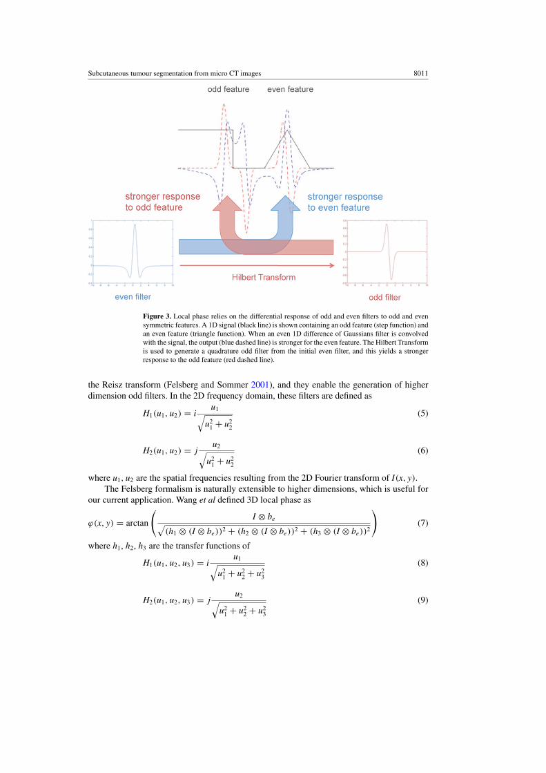
Local phase is a commonly used concept for detecting features in 1D signal processing inan intensity-invariant manner. A suitably chosen even bandpass filter, be(t), and its HilbertTransform, bo(t), which is odd, can be applied to a signal f (t) to yield information on itsshape (local phase, ϕ) and magnitude (local energy) at any given point. The local phase of a1D signal f (t) is defined in Boukerroui et al (2004) as

ϕ(t) = arctan

(be(t) ⊗ f (t)

bo(t) ⊗ f (t)

)(2)

and describes the differential response of the signal to the odd and even filters (figure 3). Theresult is a measure of the odd or even symmetry of the localized signal feature. This principle

8010 R Ali et al

(a) (b) (c)

(d) (e) (f)

Figure 2. (a) Axial microCT slice of subcutaneous tumour. (b) Exclusion map highlighting airand bone (white regions). (c) Local phase map highlighting faint boundary features (yellow spots).(d) Gradient map. ((e), (f)) Segmentation result from algorithm (red contour) superimposed onmicroCT image (e) and local phase map (f).

can be extended to multiple dimensions using Felsberg’s Monogenic Signal framework(Felsberg and Sommer 2001), where it is used as an intensity-invariant image-based featuredetector.

The bandpass filter is generated using a rotationally invariant filter (Mellor andBrady 2005),

be(r) = 1

rα+β− 1

rα−β(3)

where α = 3.25 and β = 0.25. Using this, local phase ϕ is computed as described in Mellorand Brady (2005), using the equation

ϕ(x, y) = arctan

(I ⊗ be√

(h1 ⊗ (I ⊗ be))2 + (h2 ⊗ (I ⊗ be))2

)(4)

where I is the image, be is the even bandpass filter, and h1, h2 are vector-valued filters whichgenerate a quadrature pair of odd filters when convolved with the even bandpass filter. Thesevector-valued filters are generated using an extension of the Hilbert transform known as

Subcutaneous tumour segmentation from micro CT images 8011

Figure 3. Local phase relies on the differential response of odd and even filters to odd and evensymmetric features. A 1D signal (black line) is shown containing an odd feature (step function) andan even feature (triangle function). When an even 1D difference of Gaussians filter is convolvedwith the signal, the output (blue dashed line) is stronger for the even feature. The Hilbert Transformis used to generate a quadrature odd filter from the initial even filter, and this yields a strongerresponse to the odd feature (red dashed line).

the Reisz transform (Felsberg and Sommer 2001), and they enable the generation of higherdimension odd filters. In the 2D frequency domain, these filters are defined as

H1(u1, u2) = iu1√

u21 + u2

2

(5)

H2(u1, u2) = ju2√

u21 + u2

2

(6)

where u1, u2 are the spatial frequencies resulting from the 2D Fourier transform of I(x, y).The Felsberg formalism is naturally extensible to higher dimensions, which is useful for

our current application. Wang et al defined 3D local phase as

ϕ(x, y) = arctan

(I ⊗ be√

(h1 ⊗ (I ⊗ be))2 + (h2 ⊗ (I ⊗ be))2 + (h3 ⊗ (I ⊗ be))2

)(7)

where h1, h2, h3 are the transfer functions of

H1(u1, u2, u3) = iu1√

u21 + u2

2 + u23

(8)

H2(u1, u2, u3) = ju2√

u21 + u2

2 + u23

(9)

8012 R Ali et al

Figure 4. An axial microCT slice of a subcutaneous tumour (left), and its corresponding localphase map (right). The faint interface features highlighted with red arrows on the microCT imageare emphasized in the local phase image as yellow/blue dots.

H3(u1, u2, u3) = ku3√

u21 + u2

2 + u23

(10)

thus allowing local phase to be computed on volumetric data (Wang et al 2009). Figure 4shows the local phase map for a single slice from a microCT volume, and it can be seen thatfaint features at the interface between the tumour and body are highlighted in blue.

2.4. Level set segmentation

A 3D level set is used to segment the tumour boundary using a combination of the localphase and exclusion maps, based on the implementations described in Lefohn et al (2004) andMostofi (2009). A signed distance function φ is initialized using a user input click within thetumour volume, and this is evolved using the level set PDE

∂φ

∂t= −‖∇φ‖

[αF + (1 − α)∇ · ∇φ

‖∇φ‖]

(11)

where α is a weighting coefficient for the two terms. The second term defines the regularizingcurvature term, which enforces a smoothness constraint on the boundary. The F term withinthe bracket describes an image-based speed term where

F ={ε − |ϕ − T | + β∇I if Iex = 00 otherwise

(12)

where ϕ is the local phase map (equation (7)), T defines a target threshold local phase value,ε defines a margin around that threshold, Iex is the thresholded microCT image defined inequation (1) and β is a weighting factor for the gradient term. If the level set boundary lies ona voxel whose local phase value lies within (T − ε) < T < (T + ε) then it will experience apositive growth force at that point, otherwise it will experience a negative shrinking force. Theexclusion map Iex causes the level set to experience no force if it ventures out into the excludedregions (air and bone). In these instances, it will undergo smoothing (and a slight amount ofshrinkage) due to the curvature term. The gradient term is used because the local phase of thetumour–muscle interface features are of a similar value to the tumour–air perimeter voxels,and therefore the speed term is boosted in this region to encourage the level set to extend tothe tumour–air boundary. A sample gradient map is shown in figure 2(d).

Subcutaneous tumour segmentation from micro CT images 8013

INPUT

SPEED FUNCTION

INPUT

Figure 5. Outline of segmentation algorithm.

Table 1. Summary of parameters for the CT tumour segmentation algorithm. MicroCT data andlocal phase maps are normalized to range 0–1.

Parameter Symbol Approximate value

CT air threshold ta 0.1CT bone threshold tb 0.9Level set weighting α 0.65Local phase margin ε 0.15Local phase threshold T 0.9Gradient map contribution β 5.0

The level set equation is solved in C using upwind differencing (Osher and Fedkiw 2002)and the narrow-band implementation described by Lefohn et al (2004). The parameters usedare shown in table 1. Most of the parameters are determined via observation of the microCTimage and local phase data values for the boundary features, however optimization is performedfor α and β by comparing outputs for a range of values (0.55 < α < 0.75 and 0 < β < 10).The segmentation algorithm is written in Matlab using a GUIDE-based interface for simpleuser operation, and the level set is called through a MEX function. The whole algorithm issummarized in figure 5.

2.5. Validation

The segmentation results are assessed by comparison against manually segmented tumours.The manual contours were drawn by a radiation oncology resident with experience in CTtumour segmentation, using image features that defined the surgical flat plane (the interfacebetween the tumour and muscle tissue layers). Each manual segmentation is accompaniedwith a confidence value between 1–5 which represents the resident’s confidence in identifyingthe correct boundary. Low confidence values of 1–2 were due to small or irregular tumourswith few flat plane features, or tumours that were proximal to a forelimb. High values of 4–5were due to large tumours and/or excellent flat plane features. The software used for manualcontouring was Amira 5.4.3 software (Visualization Sciences Group, Burlington, MA, USA).

The Dice similarity metric (Dice 1945) is computed to determine the level of agreementbetween the algorithm output and the manually drawn tumour boundaries. Given twosegmentation regions A and B, the Dice measure is given by

8014 R Ali et al

(a) (b)

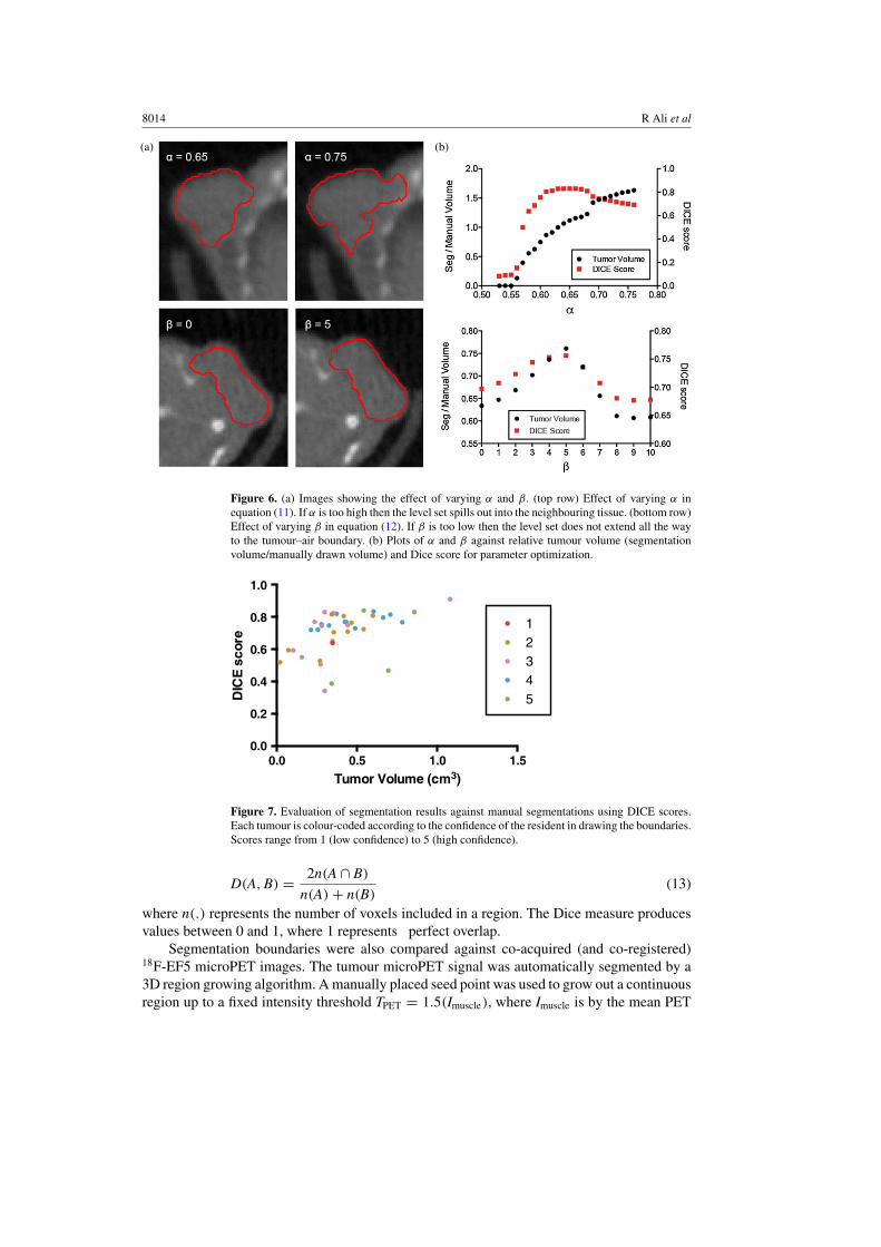
Figure 6. (a) Images showing the effect of varying α and β. (top row) Effect of varying α inequation (11). If α is too high then the level set spills out into the neighbouring tissue. (bottom row)Effect of varying β in equation (12). If β is too low then the level set does not extend all the wayto the tumour–air boundary. (b) Plots of α and β against relative tumour volume (segmentationvolume/manually drawn volume) and Dice score for parameter optimization.

Tumor Volume (cm3)

DIC

E s

core

0.0 0.5 1.0 1.50.0

0.2

0.4

0.6

0.8

1.0

12345

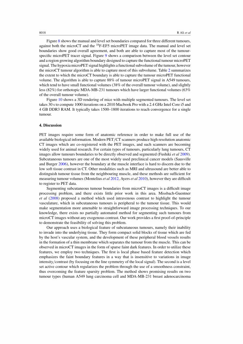
Figure 7. Evaluation of segmentation results against manual segmentations using DICE scores.Each tumour is colour-coded according to the confidence of the resident in drawing the boundaries.Scores range from 1 (low confidence) to 5 (high confidence).

D(A, B) = 2n(A ∩ B)

n(A) + n(B)(13)

where n(.) represents the number of voxels included in a region. The Dice measure producesvalues between 0 and 1, where 1 represents perfect overlap.

Segmentation boundaries were also compared against co-acquired (and co-registered)18F-EF5 microPET images. The tumour microPET signal was automatically segmented by a3D region growing algorithm. A manually placed seed point was used to grow out a continuousregion up to a fixed intensity threshold TPET = 1.5(Imuscle), where Imuscle is by the mean PET

Subcutaneous tumour segmentation from micro CT images 8015

Figure 8. Comparison between segmentation results (red contour) against manual segmentations(green contour) and tumour PET tracer uptake for three different A549 subcutaneous tumours (oneper column). Top row shows axial microCT slices of the tumour. Middle row shows the sameslice with the segmentation contours superimposed. Bottom row shows co-registered PET imageof 18F-EF5 uptake in the tumours, with segmentation contours superimposed.

intensity (defined as % injected dose per unit volume) in a reference muscle. This approachmimics the approach used clinically in defining hypoxic regions from hypoxia PET tracerdata using a tumour–muscle ratio of 1.5 (Komar et al 2008).

3. Results

Figure 2 shows the output from each step of the algorithm. The white regions in the exclusionmap (figure 2(b)) dictate no-go areas for the level set. The local phase map (figure 2(c))shows the tumour and tissue in red (0.8 � ϕ � 0.95), and the level set parameters ε andT are set to grow in these regions. The interface features are represented in the local phase

map as blue regions (ϕ � 0.6). The tumour–air boundary voxels have similar local phasevalues (0.5 � ϕ � 0.7), corresponding to the relatively dark layer of tumour voxels on the

8016 R Ali et al

Figure 9. Comparison between the CT tumour segmentation result (green contour) and a regiongrowing algorithm for segmenting the tumour PET signal (red contour in top CT image, whitecontour in bottom PET image). Top row shows axial microCT slices of the tumour, and bottomrow shows co-registered PET image. Left column shows 18F-FAZA uptake in an orthotopic MDA-MB-231 tumour, and right column shows 18F-EF5 uptake in an A549 subcutaneous tumour.

Table 2. Quantitation of percentage of functional tumour microPET region captured by CT tumoursegmentation, and size of tumour microPET region as a percentage of the microCT-derived volume.n represents number of tumours analysed.

Tumour type Tracer % PET region captured Fraction of CT volume n

A549 18F-EF5 87.9 ± 2.7 37.8 ± 13.7 15MDA-MB-231 18F-FAZA 81.8 ± 15.1 63.1 ± 24.1 8

air boundary due to partial volume effect, and this causes the level set to terminate early. Tocounteract this, the gradient map (figure 2(d)) is added to the local phase map to raise the valuesof the air boundary voxels, thus encouraging the level set to propagate to the true boundary.

Figures 2(e) shows the results of the level set (red contour) superimposed over the originalmicroCT image, and figure 2(f) shows the level set result superimposed on the local phasemap. The level set is clearly arrested when it encounters the local phase boundary features,and the curvature term prevents it from leaking out from the edges where fewer features areavailable.

Subcutaneous tumour segmentation from micro CT images 8017

Figure 10. Birds-eye view 3D volume rendering of the segmentation results (red) superimposedon the microCT image (grey) for two mice.

The effect of the key parameters is shown in figure 6. Two parameters are optimized, α

in equation (11) and β in equation (12). The most important term is α, the speed functiontuning parameter which determines the relative contribution of the local phase map and thecurvature term. When α is too high, the local phase term dominates and the level set spills outinto the neighbouring tissues. Conversely, when α is too low, the curvature term dominatesand the level set undergoes a net shrinkage. The plot in figure 6(b) shows that α is relativelyinsensitive to small variations around the optimal value (α ± 0.05), but the segmentationquality degrades rapidly outside this range. The second term, β, controls the gradient mapweight. When β is close to zero, the level set does not reach the tumour–air boundary. Theoptimum value is found around β = 5, although the algorithm is relatively insensitive tovariations in β. The parameter values in table 1 were found to work with most of the analysedtumours, with minor variations in α yielding improvements in some cases.

Figure 7 summarizes the segmentation results against manual segmentations (n = 39) forA549 subcutaneous tumours. When compared against manual segmentations, the algorithmachieves consistently high Dice scores (mean Dice score is 0.71; 95% confidence interval is0.67–0.75) across a range of tumour volumes (range 0.1–1.1 cm3). The algorithm is able toperform well in simple and difficult cases (as determined by the resident’s confidence in eachcontour). Six tumours obtain Dice scores less than 0.5. Examination of these tumours revealstwo causes of the low scores. The first is that the algorithm underestimates the manually drawnboundary, and in the case of small tumours, this results in a higher proportion of false-negativevoxels which impacts the score. The second is that the level set overshot the true boundarydue to a lack of strong tumour–tissue interface features to constrain it.

8018 R Ali et al

Figure 8 shows the manual and level set boundaries compared for three different tumours,against both the microCT and the 18F-EF5 microPET image data. The manual and level setboundaries show good overall agreement, and both are able to capture most of the tumour-specific microPET tracer signal. Figure 9 shows a comparison between the level set contourand a region growing algorithm boundary designed to capture the functional tumour microPETsignal. The hypoxia microPET signal highlights a functional subvolume of the tumour, howeverthe microCT tumour algorithm is able to capture most of this subvolume. Table 2 summarizesthe extent to which the microCT boundary is able to capture the tumour microPET functionalvolume. The algorithm is able to capture 88% of tumour microPET signal in A549 tumours,which tend to have small functional volumes (38% of the overall tumour volume), and slightlyless (82%) for orthotopic MDA-MB-231 tumours which have larger functional volumes (63%of the overall tumour volume).

Figure 10 shows a 3D rendering of mice with multiple segmented tumours. The level settakes 30 s to compute 1000 iterations on a 2010 Macbook Pro with a 2.4 GHz Intel Core i5 and4 GB DDR3 RAM. It typically takes 1500–1800 iterations to reach convergence for a singletumour.

4. Discussion

PET images require some form of anatomic reference in order to make full use of theavailable biological information. Modern PET/CT scanners produce high resolution anatomicCT images which are co-registered with the PET images, and such scanners are becomingwidely used for animal research. For certain types of tumours, particularly lung tumours, CTimages allow tumours boundaries to be directly observed and segmented (Fushiki et al 2009).Subcutaneous tumours are one of the most widely used preclinical cancer models (Sausvilleand Burger 2006), however the boundary at the muscle interface is hard to discern due to thelow soft tissue contrast in CT. Other modalities such as MRI and ultrasound are better able todistinguish tumour tissue from the neighbouring muscle, and these methods are sufficient formeasuring tumour volumes (Montelius et al 2012, Ayers et al 2010), however they are difficultto register to PET data.

Segmenting subcutaneous tumour boundaries from microCT images is a difficult imageprocessing problem, and there exists little prior work in this area. Missbach-Guentneret al (2008) proposed a method which used intravenous contrast to highlight the tumourvasculature, which in subcutaneous tumours is peripheral to the tumour tissue. This wouldmake segmentation more amenable to straightforward image processing techniques. To ourknowledge, there exists no partially automated method for segmenting such tumours frommicroCT images without any exogenous contrast. Our work provides a first proof-of-principleto demonstrate the feasibility of solving this problem.

Our approach uses a biological feature of subcutaneous tumours, namely their inabilityto invade into the underlying tissue. They form compact solid blocks of tissue which are fedby the host’s vascular system, and the development of these peripheral blood vessels resultsin the formation of a thin membrane which separates the tumour from the muscle. This can beobserved in microCT images in the form of sparse faint dark features. In order to utilize thesefeatures, we employ two techniques. The first is local phase based feature detection whichemphasizes the faint boundary features in a way that is insensitive to variations in imageintensity/contrast (by focusing on the line symmetry of the local signal). The second is a levelset active contour which regularizes the problem through the use of a smoothness constraint,thus overcoming the feature sparsity problem. The method shows promising results on twotumour types (human A549 lung carcinoma cell and MDA-MB-231 breast adenocarcinoma

Subcutaneous tumour segmentation from micro CT images 8019

xenografts) and a single scanner (a Siemens Inveon microPET/CT). Further development ofthis method will require testing on different tumour types and images from different scanners.

The algorithm is available as open-source software from www.setuvo.com. There existsconsiderable scope for improvements. GPU-based techniques can be used to improve the speedof the level set computation, and the initialization methods can also be improved (using, forexample, co-acquired PET data). The accuracy can be improved through the incorporationof additional prior information based on an improved understanding of the tumour modelsbeing imaged. Our future work involves using the segmentation boundaries as an input formathematical models of tumour growth, thus providing tumour boundary conditions for themodels. Other uses can include the development of PET tumour quantification metrics whichinclude the contribution from PET-negative tumour voxels, for example tumour hypoxicfraction when imaging with hypoxia-specific PET tracers.

Acknowledgments

The authors would like to thank the funding providers which include the Stanford MolecularImaging Scholars program (NIH/NCI R25 CA118681-06) which funded RA, and NIH/NCIR01 CA131199 which funded the imaging studies.

References

Ayers G D et al 2010 Volume of preclinical xenograft tumors is more accurately assessed by ultrasound imaging thanmanual caliper measurements J. Ultrasound Med. 29 891–901

Boukerroui D, Brady M and Noble A 2004 On the choice of band-pass quadrature filters J. Math. Imaging Vis. 21 53–80Dice L 1945 Measures of the amount of ecologic association between species Ecology 26 297–302Felsberg M and Sommer G 2001 The monogenic signal IEEE Trans. Signal Process. 49 3136–44Fushiki H, Kanoh-Azuma T, Katoh M, Kawabata K, Jiang J, Tsuchiya N, Satow A, Tamai Y and Hayakawa Y

2009 Quantification of mouse pulmonary cancer models by microcomputed tomography imaging CancerSci. 100 1544–9

Komar G, Seppanen M, Eskola O, Lindholm P, Gronroos T J, Forsback S, Sipila H, Evans S M, Solin O and Minn H2008 18F-EF5: a new PET tracer for imaging hypoxia in head and neck cancer J. Nucl. Med. 49 1944–51

Lefohn A E, Kniss J M, Hansen C D and Whitaker R T 2004 A streaming narrow-band algorithm: interactivecomputation and visualization of level sets IEEE Trans. Vis. Comput. Graphics 10 422–33

Mellor M and Brady M 2005 Phase mutual information as a similarity measure for registration Med. ImageAnal. 9 330–43

Missbach-Guentner J, Dullin C, Tomography C, Kimmina S, Zientkowska M, Domeyer-Missbach M and Malz C2008 Morphologic changes of mammary carcinomas in mice over time as monitored by flat-panel detectorvolume Neoplasia 10 663–73

Montelius M, Ljungberg M, Horn M and Forssell-Aronsson E 2012 Tumour size measurement in a mouse modelusing high resolution MRI BMC Med. Imaging 12 12

Mostofi H 2009 Fast level set segmentation of biomedical images using graphics processing units PhD ThesisUniversity of Oxford, UK

Osher S and Fedkiw R 2002 Level Set Methods and Dynamic Implicit Surfaces (Berlin: Springer)Sausville E A and Burger A M 2006 Contributions of human tumor xenografts to anticancer drug development Cancer

Res. 66 3351–4 (discussion 3354)Wang P, Kelly C and Brady M 2009 Application of 3D local phase theory in vessel segmentation ISBI’09: 6th IEEE

Int. Symp. on Biomedical Imaging pp 1174–7