SELF-VALIDATING OPTIMUM CURRENCY AREAS∗

GIANCARLO CORSETTI

University of Rome III, Yale University and CEPR

PAOLO PESENTI

International Monetary Fund,

Federal Reserve Bank of New York and NBER

First Draft: December 2001

Revised: May 2002

Abstract

A currency area can be a self-validating optimal policy regime, evenwhen monetary unification does not foster real economic integration andintra-industry trade. In our model, firms choose the optimal degree ofexchange rate pass-through to export prices while accounting for expectedmonetary policies, and monetary authorities choose optimal policy ruleswhile taking firms’ pass-through as given. We show that there exist twoequilibria, each of which defines a self-validating currency regime. In thefirst, firms preset prices in domestic currency and let prices in foreigncurrency be determined by the law of one price. Optimal policy rulesthen target the domestic output gap, and floating exchange rates supportthe flex-price allocation. In the second equilibrium, firms preset prices inconsumer currency, and a monetary union is the optimal policy choice forall countries. Although a common currency helps synchronize businesscycles across countries, flexible exchange rates deliver a superior welfareoutcome.

JEL classification: E5, F4Keywords: optimum currency areas, monetary union, optimal cyclical

monetary policy, nominal rigidities, exchange rate pass-through.

∗We thank Luca Dedola, Rudi Dornbusch, Petra Geraats, Maury Obstfeld, Ken Rogoff,Cedric Tille and seminar participants at the 2002 AEA Meetings in Atlanta, the 2002 SummerSymposium for Central Bank Researchers at Gerzensee, the Board of Governors of the FederalReserve System, the University of Virginia, and the Johns Hopkins SAIS for many helpfulcomments. We also thank Raymond Guiteras for excellent research assistance. Corsetti’swork on this paper is part of a research network on “The Analysis of International CapitalMarkets: Understanding Europe’s Role in the Global Economy,Ô funded by the EuropeanCommission under the Research Training Network Programme (Contract No. HPRN-CT-1999-00067). The views expressed here are those of the authors, and do not necessarily reflectthe position of the International Monetary Fund, the Federal Reserve Bank of New York, theFederal Reserve System, or any other institution with which the authors are affiliated.

I Introduction

The theory of optimum currency areas (OCAs), from the classic contributions

by Mundell [1961], McKinnon [1963], Kenen [1969] and Ingram [1973] to its

modern applications and revisions,1 stresses that asymmetric, country-specific

shocks represent a key element in the choice of exchange rate regime. Specifi-

cally, asymmetric real shocks weaken the case for a common currency, as mem-

ber states of a monetary union lose their ability to use domestic exchange rate

and interest rate policies for stabilization purposes. Conversely, business cycle

synchronization and macroeconomic convergence make a currency area an opti-

mal monetary arrangement, other things being equal, by reducing the scope for

asymmetric policy responses to the disturbances hitting the union-wide econ-

omy.

Monetary union may nonetheless become optimal ex post, even though the

individual countries that join it do not meet the optimality criteria ex ante.

In the vast literature on optimum currency areas, the argument for an endoge-

nous optimal currency area emphasizes that the monetary union itself could act

as a catalyst of business cycle synchronization. An influential contribution by

Frankel and Rose [1997, 1998] suggests that the reduction of foreign exchange

transaction costs promotes trade integration across countries: to the extent

that the process of integration enhances intra-industry trade rather than prod-

uct specialization, national business cycles become more synchronized, since

sectoral demand shocks and productivity innovations affect all countries at the

same time. Higher national output correlation then reduces the need for ex-

change rate adjustments to stabilize national employment and prices, and min-

imizes the welfare costs of giving up national currencies. Not everyone agrees

with this argument: for instance Eichengreen [1992] and Krugman [1993] stress

that monetary integration could lead to greater specialization in production,

thus lowering output correlation and making regions more vulnerable to local

shocks. On an empirical basis, however, the evidence presented by Frankel and

Rose [1997, 1998] supports the view that trade links raise income correlations.

1Those include, among others, Eichengreen [1990, 1992], Dowd and Greenaway [1993],

Tavlas [1993], Bayoumi and Eichengreen [1994], Melitz [1996], Bayoumi [1997], and Alesina

and Barro [2002]. See Buiter, Corsetti and Pesenti [1998], ch.10, for a critical survey of the

literature.

1

Moreover, Rose and Engel [2000] show that membership in a common currency

area increases international business cycle correlations by a significant amount.

But what if monetary integration fails to boost economic convergence and

intra-industry trade? Would it still be possible for a monetary union to satisfy

ex post the OCA criterion when monetary and real integration fail to move in

tandem? In this paper, we offer a distinct argument for a theory of endoge-

nous optimal currency areas, with conceptual roots in the Lucas critique. We

show that — independent of economic integration — the adoption of a common

monetary policy can be self-validating: when the private sector chooses pricing

strategies that are optimal in a monetary union, such strategies make a cur-

rency area the optimal monetary regime from the vantage point of the national

policymakers as well. In other words, there is no incentive for monetary au-

thorities to pursue independent strategies of national output stabilization. As

a result, even if there is no structural change in fundamentals (e.g., no increase

in intra-industry trade), national outputs become more correlated.

We analyze endogenous optimal monetary unions within a general-equilibrium

two-country, choice-theoretic stochastic setting where national welfare is mea-

sured by the utility of each country’s representative household.2 The key ele-

ments of our approach are imperfect competition in production, nominal rigidi-

ties in the goods markets, and forward-looking price-setting by firms. Drawing

on Corsetti and Pesenti [2001a], our setup allows for imperfect pass-through of

exchange rate onto export prices. In what follows, the degree of pass-through

is endogenously chosen ex ante by exporters, in the form of a rule of limited

price flexibility contingent on exchange rate movements.

To distinguish our theory from the previous argument for endogenous op-

timal currency areas, we rule out a priori structural change: countries are

perfectly specialized in the production of one type of good before and after the

monetary union. Firms optimally choose prices and pass-through elasticities

based on information on shocks and policy rules. Taking firms’ pricing and

pass-through strategies as given, monetary authorities choose optimal state-

contingent policy rules. In a world equilibrium, both the degree of pass-through

2Other contributions in the recent literature include Obstfeld and Rogoff [2000, 2002],

Devereux and Engel [2000], Corsetti and Pesenti [2001a], Benigno [2001], Clarida, Gali and

Gertler [2001], Canzoneri, Cumby and Diba [2002]. On the welfare effects of a currency area

when political factors influence monetary policy see Neumeyer [1998].

2

and monetary policy are jointly determined by optimizing agents.

We show that there are two equilibria, which can be Pareto ranked. While

exporters could in principle choose any intermediate level of pass-through, in

equilibrium pass-through is either 100 percent or zero as producers optimally

choose ‘corner’ pricing strategies to prevent their markups from being affected

by exchange rate fluctuations.3 There is one equilibrium in which firms choose

to preset prices in domestic currency, and let the foreign price adjust according

to the law of one price. With complete pass-through, monetary policies are fully

inward-looking: they implement stabilization rules that close national output

gaps completely in every period. This equilibrium is inconsistent with fixed

exchange rates, and implies low correlation among output levels — depending

on the cross-country correlation of fundamental shocks. The exchange rate plays

the role stressed by Friedman [1953]: it brings about the required relative price

adjustments that are hindered by the presence of nominal price rigidities.

But there is another equilibrium in which firms preset prices in consumer

currency. With zero pass-through in the world economy, monetary policies are

perfectly symmetric across countries, that is, they both respond to the same

average of national shocks. This equilibrium is consistent with an OCA: there

is no cost in giving up monetary sovereignty because, even if national mone-

tary authorities remained independent, they would still choose to implement

the same policy rules, moving interest rates in tandem and responding sym-

metrically to world-wide shocks. National outputs are perfectly correlated even

when shocks are asymmetric.

In welfare terms, the optimal monetary union is Pareto-inferior to the Friedman-

style arrangement in the first equilibrium. Although the private and the public

sector ‘do the right thing’ — in terms of policy and pricing strategies — once

the equilibrium with a monetary union is selected, there is still room for welfare

improvement by creating conditions for relative price adjustment via changes

of the exchange rate. A move toward more volatile rates and less synchronized

business cycles would bring about the appropriate change in firms’ pricing and

pass-through strategies, which in turn would validate the floating regime as

optimal.

3Related literature focuses on the choice of pricing strategies where monetary authorities

are assumed to implement non-optimizing, noisy policies (as in the work by Bacchetta and

Van Wincoop [2001] and Devereux and Engel [2001]) rather than optimal rules.

3

This paper is organized as follows. Section 2 develops the model. Section 3

studies price-setters’ optimal behavior and endogenous pass-through strategies

for given monetary policies. Section 4 focuses instead on optimal monetary

policies given firms’ pricing strategies. The previous two pieces of analysis are

brought together in sections 5 and 6, which characterize the equilibrium of the

economy. A final section discusses our main results.

II The model

A Preferences, technology and budget constraints

We model a world economy with two countries, H (Home) and F (Foreign), each

specialized in one type of traded good. Each good is produced in a number of

brands defined over a continuum of unit mass. Brands are indexed by h in

the Home country and f in the Foreign country. Each country is populated by

households defined over a continuum of unit mass. Households are indexed by

j in the Home country and j∗ in the Foreign country.

Home agent j’s lifetime expected utility W is defined as:

(1) Wt−1(j) ≡ Et−1

∞∑

τ=t

βτ−t [lnCτ (j)− κ`τ (j)] 0 < β < 1, κ > 0

where β is the discount rate. The instantaneous utility is a positive function of

the consumption index C(j) and a negative function of labor effort `(j). Foreign

agents’ preferences are similarly defined: the discount rate is the same as in the

Home country, while κ∗ in the Foreign country need not coincide with κ in the

Home country.

For each agent j in the Home country, the consumption indexes of Home

and Foreign brands are defined as:

(2)

CH,t(j) ≡[∫ 1

0Ct(h, j)

θ−1θ dh

]θ

θ−1

, CF,t(j) ≡[∫ 1

0Ct(f, j)

θ∗−1θ∗ df

]θ∗

θ∗−1

θ, θ∗ > 1.

where Ct(h, j) and Ct(f, j) are respectively consumption of Home brand h and

Foreign brand f by Home agent j at time t. Each Home brand is an imperfect

substitute for all other Home brands, with constant elasticity of substitution θ.

Similarly the elasticity of substitution among Foreign brands is θ∗. The con-

4

sumption indexes in the Foreign country, C∗H,t(j

∗) and C∗F,t(j

∗), are analogously

defined.

We assume that the elasticity of substitution between Home and Foreign

types is one, thus smaller than the elasticity of substitution between brands

of the same type of good produced in each country, θ and θ∗. Under this

assumption the consumption baskets of individuals j and j∗ can be written as

a Cobb-Douglas function of the Home and Foreign consumption indexes:

(3) Ct(j) ≡ CH,t(j)γCF,t(j)

1−γ , C∗t (j

∗) ≡ C∗H,t(j

∗)γC∗F,t(j

∗)1−γ 0 < γ < 1

where the weights γ and 1− γ are identical across countries.

We denote the prices of brands h and f in the Home market (thus expressed

in the Home currency) as p(h) and p(f), and the prices in the Foreign market

(in Foreign currency) as p∗(h) and p∗(f). Given the prices of brands, we can

derive the utility-based price indexes PH, PF, P and their Foreign analogs.4 In

particular, the utility-based CPIs are:

(4) Pt =P γH,tP

1−γF,t

γW

, P ∗t =

(

P ∗H,t

)γ (P ∗F,t

)1−γ

γW

γW ≡ γγ(1− γ)1−γ .

Each brand h is produced by a single Home agent and sold in both countries

under conditions of monopolistic competition. Output is denoted Y . Technology

is linear in household’s h labor, `(h). The resource constraint for brand h is:

(5) Yt(h) =`t(h)

αt≥

∫ 1

0Ct(h, j)dj +

∫ 1

0C∗

t (h, j∗)dj∗

where α is a country-specific productivity shock. The resource constraint for

Foreign brand f is similarly defined as a function of the productivity shock in

the Foreign country, α∗.

Home agent j receives a revenue R(j) from the sale of the good she produces.

Since each agent is the sole producer of a specific brand, we associate individual

j with brand h. The sales revenue of agent j, expressed in Home currency, is:

(6) Rt(j) ≡ pt(h)

∫ 1

0Ct(h, j)dj + Etp∗t (h)

∫ 1

0Ct(h, j

∗)dj∗

4For instance, the utility-based price index PH,t is defined as the minimum expen-

diture required to buy one unit of the composite good CH,t and is derived as PH,t =[

∫ 10 pt(h)1−θdh

] 11−θ

.

5

where E is the nominal exchange rate, defined as Home currency per unit of

Foreign currency.

Home agents hold two international bonds, BH and BF, denominated in

Home and Foreign currency, respectively.5 Both international bonds are in zero

net supply. The individual flow budget constraint for agent j in the Home

country is:

BH,t+1(j) + EtBF,t+1(j) ≤ (1 + it)BH,t(j) + (1 + i∗t )EtBF,t(j)

+Rt(j)−∫ 1

0pt(h)Ct(h, j)dh−

∫ 1

0pt(f)Ct(f, j)df(7)

In the expression above the short-term nominal rates it and i∗t are paid at the

beginning of period t and are known at time t − 1. The two short-term rates

are directly controlled by the national governments.6 Similar expressions hold

for the Foreign country, after associating household j∗ with brand f .

Taking prices as given, Home agent j maximizes (1) subject to (7) with

respect to consumption and asset holdings. A similar optimization problem is

solved by Foreign agent j∗. In our analysis below we focus on symmetric equilib-

ria in which at some initial point in time t = 0 all agents have zero net financial

wealth. As shown in Corsetti and Pesenti [2001a, b], in equilibrium both wealth

and the current account are endogenously zero at any subsequent point in time:

Home imports from Foreign are always equal in value to Foreign imports from

Home. Since agents are equal within countries (though not necessarily symmet-

ric across countries) we can drop the indexes j and j∗ and interpret all variables

in per-capita (or aggregate) terms. As trade and the current account are always

balanced, countries consume precisely their aggregate sales revenue:

(8) Rt − PtCt = 0, R∗t − P ∗

t C∗t = 0.

5We adopt the notation of Obstfeld and Rogoff [1996, ch.10]. Specifically, our timing

convention has BH,t(j) and BF,t(j) as agent j’s nominal bonds accumulated during period

t− 1 and carried over into period t.6The adoption of a cash-less economy framework is merely motivated in terms of analytical

convenience. All the results of this model go through when money demand is explicitly

considered. Liquidity demand could easily be introduced in the model through a cash-in-

advance constraint of the type Mt(j) = PtCt(j) and M∗t (j) = P ∗

t C∗t (j

∗), or through a

money-in-utility-function framework. In both cases the money stock would be residually

determined in equilibrium as a function of nominal interest rates.

6

B Nominal rigidities, exchange rate pass-through and price

setting

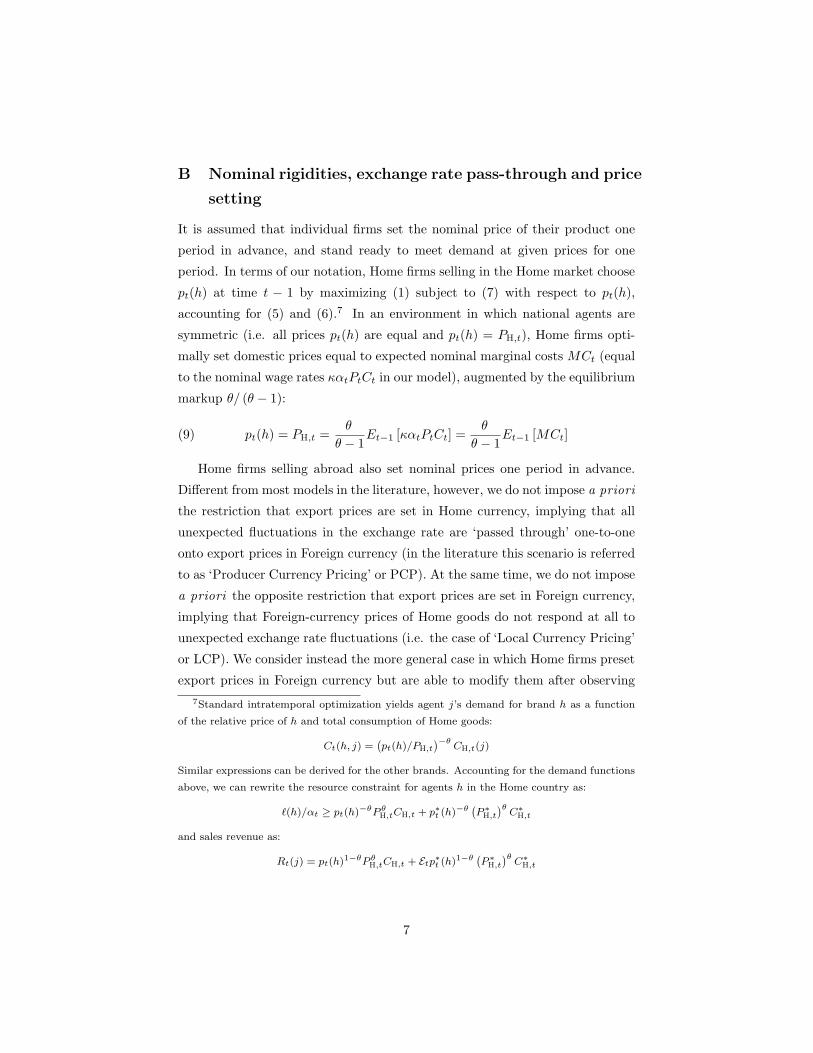
It is assumed that individual firms set the nominal price of their product one

period in advance, and stand ready to meet demand at given prices for one

period. In terms of our notation, Home firms selling in the Home market choose

pt(h) at time t − 1 by maximizing (1) subject to (7) with respect to pt(h),

accounting for (5) and (6).7 In an environment in which national agents are

symmetric (i.e. all prices pt(h) are equal and pt(h) = PH,t), Home firms opti-

mally set domestic prices equal to expected nominal marginal costs MCt (equal

to the nominal wage rates καtPtCt in our model), augmented by the equilibrium

markup θ/ (θ − 1):

(9) pt(h) = PH,t =θ

θ − 1Et−1 [καtPtCt] =

θ

θ − 1Et−1 [MCt]

Home firms selling abroad also set nominal prices one period in advance.

Different from most models in the literature, however, we do not impose a priori

the restriction that export prices are set in Home currency, implying that all

unexpected fluctuations in the exchange rate are ‘passed through’ one-to-one

onto export prices in Foreign currency (in the literature this scenario is referred

to as ‘Producer Currency Pricing’ or PCP). At the same time, we do not impose

a priori the opposite restriction that export prices are set in Foreign currency,

implying that Foreign-currency prices of Home goods do not respond at all to

unexpected exchange rate fluctuations (i.e. the case of ‘Local Currency Pricing’

or LCP). We consider instead the more general case in which Home firms preset

export prices in Foreign currency but are able to modify them after observing

7Standard intratemporal optimization yields agent j’s demand for brand h as a function

of the relative price of h and total consumption of Home goods:

Ct(h, j) =(

pt(h)/PH,t

)−θCH,t(j)

Similar expressions can be derived for the other brands. Accounting for the demand functions

above, we can rewrite the resource constraint for agents h in the Home country as:

`(h)/αt ≥ pt(h)−θP θ

H,tCH,t + p∗t (h)−θ

(

P ∗H,t

)θC∗

H,t

and sales revenue as:

Rt(j) = pt(h)1−θP θ

H,tCH,t + Etp∗t (h)1−θ(

P ∗H,t

)θC∗

H,t

7

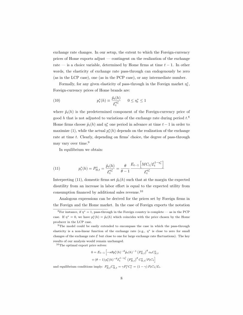
exchange rate changes. In our setup, the extent to which the Foreign-currency

prices of Home exports adjust — contingent on the realization of the exchange

rate — is a choice variable, determined by Home firms at time t − 1. In other

words, the elasticity of exchange rate pass-through can endogenously be zero

(as in the LCP case), one (as in the PCP case), or any intermediate number.

Formally, for any given elasticity of pass-through in the Foreign market η∗t ,

Foreign-currency prices of Home brands are:

(10) p∗t (h) ≡pt(h)

Eη∗t

t

0 ≤ η∗t ≤ 1

where pt(h) is the predetermined component of the Foreign-currency price of

good h that is not adjusted to variations of the exchange rate during period t.8

Home firms choose pt(h) and η∗t one period in advance at time t− 1 in order to

maximize (1), while the actual p∗t (h) depends on the realization of the exchange

rate at time t. Clearly, depending on firms’ choice, the degree of pass-through

may vary over time.9

In equilibrium we obtain:

(11) p∗t (h) = P ∗H,t =

pt(h)

Eη∗t

t

=θ

θ − 1

Et−1

[

MCt/E1−η∗

tt

]

Eη∗t

t

Interpreting (11), domestic firms set pt(h) such that at the margin the expected

disutility from an increase in labor effort is equal to the expected utility from

consumption financed by additional sales revenue.10

Analogous expressions can be derived for the prices set by Foreign firms in

the Foreign and the Home market. In the case of Foreign exports the notation

8For instance, if η∗ = 1, pass-through in the Foreign country is complete — as in the PCP

case. If η∗ = 0, we have p∗t (h) = pt(h) which coincides with the price chosen by the Home

producer in the LCP case.9The model could be easily extended to encompass the case in which the pass-through

elasticity is a non-linear function of the exchange rate (e.g., η∗ is close to zero for small

changes of the exchange rate E but close to one for large exchange rate fluctuations). The key

results of our analysis would remain unchanged.10The optimal export price solves:

0 = Et−1

[

−κθp∗t (h)−θ pt(h)

−1 (P ∗H,t

)θαtC

∗H,t

+(θ − 1) p∗t (h)−θE1−η∗

tt

(

P ∗H,t

)θC∗

H,t/PtCt

]

and equilibrium conditions imply: P ∗H,tC

∗H,t = γP ∗

t C∗t = (1− γ)PtCt/Et.

8

is:

(12) pt(f) = p∗t (f)Eηtt , 0 ≤ ηt ≤ 1

where the degree of pass-through in the Home country, ηt, need not be equal to

that in the Foreign country, η∗t . The optimal pricing strategy is such that:

(13) P ∗F,t =

θ∗

θ∗ − 1Et−1 [MC∗

t ] , PF,t =θ∗

θ∗ − 1Eηtt Et−1

[

MC∗t E

1−ηtt

]

Clearly, Home firms are willing to supply goods at given prices as long as

their ex-post markup does not fall below one:

(14) PH,t ≥ MCt, P ∗H,t ≥

MCt

EtOtherwise, agents would be better off by not accommodating shocks to demand.

In what follows, we restrict the set of shocks so that the ‘participation constraint’

(14) and its Foreign analog are never violated.

C Monetary policy and the closed-form solution of the

model

Before deriving the general solution of the model, it is helpful to introduce an

index of monetary stance µt such that:

(15)1

µt

= β(1 + it+1)Et

(

1

µt+1

)

or, integrating forward,

(16)1

µt

= Et limN→∞

βN 1

µt+N

N−1∏

τ=0

(1 + it+τ+1)

This expression shows that the index of monetary stance is a function of both

current and future expected Home nominal interest rates: Home monetary eas-

ing at time t (a higher µt) reflects either an interest rate cut at time t (i.e., a

lower it+1) or expectations of future interest rates cuts. A similar expression

holds for the Foreign country.

Note that in equilibrium µt is equal to PtCt (and µ∗t is equal to P ∗

t C∗t ): a

monetary expansion delivers increased nominal spending.11 A monetary union

11This result can be obtained by comparing (15) with the Home Euler equation under

logarithmic utility, i.e. 1 = β (1 + it+1)Et (PtCt/Pt+1Ct+1).

9

in our framework is defined as a regime in which it+1 = i∗t+1 for all t. If both

countries adopt the same numeraire, this implies µt = µ∗t .

Table 1 presents the general solution of the model, in which all endogenous

variables (17) through (26) are expressed in closed form as functions of real

shocks (αt and α∗t ) and monetary stances (µt and µ∗

t ).12

Interpreting Table 1: since the equilibrium current account is always bal-

anced (see (8) above) and the demand for imports is proportional to nominal

expenditures PtCt and P ∗t C

∗t , the nominal exchange rate Et in (17) is propor-

tional to PtCt/P∗t C

∗t , that is, a function of the relative monetary stance.13 The

relations (18) link marginal costs to macroeconomic shocks and monetary pol-

icy. Domestic prices of domestic goods are predetermined according to (19)

and (22), while import prices vary with the exchange rate, depending on the

degree of exchange rate pass-through according to (20) and (21). Equilibrium

consumption is determined in (23) and (24). Finally employment and output14

levels are determined according to (25) and (26).

III Optimal exchange rate pass-through for given

monetary policy

What is the optimal degree of exchange rate pass-through onto export prices of

Home goods in the Foreign market? Taking monetary stances and policy rules

as given, Home firms choose η∗ as to maximize (1). In a symmetric environment

12Algebraic details can be found in the Appendix of Corsetti and Pesenti [2001a]. Note that

the solution does not hinge upon any specific assumption or restriction on the nature of the

shocks besides the participation constraints (14) and their Foreign analogues.13Recall that monetary stances µt and µ∗

t depend on current and future short-term nominal

interest rates. Hence the exchange rate, which is proportional to the ratio of µt to µ∗t , is a

forward-looking variable.14Recall that national outputs Yt and Y ∗

t are respectively equal to `t/αt and `∗t /α∗t .

10

Table 1: The closed-form solution of the model

Et =1− γ

γ

µt

µ∗t

(17)

MCt = καtµt MC∗t = κ∗α∗

tµ∗t(18)

PH,t =θ

θ − 1Et−1 (MCt)(19)

PF,t =θ∗

θ∗ − 1Eηtt Et−1

[

MC∗t E

1−ηtt

]

(20)

P ∗H,t =

θ

θ − 1

Et−1

[

MCt/E1−η∗

tt

]

Eη∗t

t

(21)

P ∗F,t

=θ∗

θ∗ − 1Et−1 (MC∗

t )(22)

Ct =

γW

(

θ − 1

θ

)γ (θ∗ − 1

θ∗

)1−γ

µtE−ηt(1−γ)t

[Et−1 (MCt)]γ[

Et−1

(

MC∗t E

1−ηtt

)]1−γ(23)

C∗t =

γW

(

θ − 1

θ

)γ (θ∗ − 1

θ∗

)1−γ

µ∗tE

η∗t γ

t

[

Et−1

(

MCt/E1−η∗t

t

)]γ

[Et−1 (MC∗t )]

1−γ

(24)

`t =

(

θ − 1

θκ

)

γMCt

Et−1 (MCt)+ (1− γ)

MCt/E1−η∗

tt

Et−1

[

MCt/E1−η∗t

t

]

(25)

`∗t =

(

θ∗ − 1

θ∗κ∗

)

(1− γ)MC∗

t

Et−1 (MC∗t )

+ γMC∗

t E1−ηtt

Et−1

[

MC∗t E

1−ηtt

]

(26)

11

with p∗(h) = P ∗H the first order condition is:15

(27) 1 =θ κ

θ − 1

Et−1

[

(αtP∗t C

∗t ln Et) /P ∗

H,t

]

Et−1 [ln Et]γ

1− γ

Comparing (27) with (11), it follows that the optimal pass-through η∗ is such

that:

(28) Et−1

[

αtµ∗tE

η∗t

t

]

=Et−1

[

αtµ∗tE

η∗t

t ln Et]

Et−1 [ln Et]

or, rearranging:

(29) Covt−1

[

MCt/E1−η∗

tt , ln Et

]

= 0

This is a key condition. At an optimum, the (reciprocal of the) markup in

the export market must be uncorrelated with the (log of the) exchange rate.

Trivially, if E is constant or fully anticipated, any degree of pass-through is

consistent with the previous expression. But if E is not perfectly predictable, the

optimal degree of pass-through will depend on the expected monetary policies

and the structure of the shocks.

This is because, in equilibrium, Home ex-post real profits in the Foreign

market16 are proportional to pt(h) − MCt/E1−η∗

tt , that is, they are a concave

15The optimal pass-through solves:

0 = Et−1

[

−κpt(h)−θθ ln Et exp {η∗t θ ln Et}

(

P ∗H,t

)θαtC

∗H,t

−Etpt(h)1−θ (1− θ) ln Et exp {−η∗t (1− θ) ln Et}(

P ∗H,t

)θC∗

H,t/PtCt

]

and equilibrium conditions imply: P ∗H,tC

∗H,t = γP ∗

t C∗t = (1− γ)PtCt/Et.

16Denoting with Πt(h) Home agent h’s ex-post real profits from selling in the Foreign

market, we can write:

Πt(h) = Qt−1,t

(

Etpt (h) E−η∗

t −MCt

)

(

pt (h)

˜PH,t

)−θ

C∗H,t

where Q is the pricing kernel and ˜PH the predetermined export price, defined as:

Qt−1,t ≡ βPt−1Ct−1

PtCt, P ∗

H,t ≡ ˜PH,tE−η∗

t

Using the equilibrium expression for C∗H and Q we obtain:

Πt(h) = β (1− γ)µt−1

˜PH,t

(

pt (h)− καtµt/E1−η∗

t

)

(

pt (h)

˜PH,t

)−θ

Note that expressions 11 and 27 can be obtained by maximizing Et−1Πt(h) with respect to

pt (h) and η∗t . See the discussion in Corsetti and Pesenti [2001a].

12

function of E for η∗ < 1.17 This implies that, keeping everything else constant,

exchange rate shocks reduce expected profits from exports. In general, however,

to assess the overall exposure of profits to exchange rate uncertainty it is crucial

to know whether or not the underlying shocks make unit export revenue and

marginal costs co-vary positively. In fact, if MC is high in those states of

nature in which pE1−η∗is high as well, exchange rate uncertainty has little or no

effect on profits. When the firm chooses the degree of pass-through, it equates

the ‘marginal costs’ of imperfect pass-through, in terms of reduced expected

revenue, with the ‘marginal benefits’ of imperfect pass through, in terms of

increased covariance between revenue and marginal costs. By the same token,

the optimal pass-through chosen by Foreign firms selling in the Home market

requires:

(30) Covt−1

(

MC∗t E

1−ηtt , ln (1/Et)

)

= 0.

To build intuition, suppose that there are no productivity shocks and the

only source of uncertainty is exogenous monetary volatility. If µ is the only

source of uncertainty, condition (29) becomes:

(31) Covt−1

[

µη∗t

t , lnµt

]

= 0

which is solved by η∗t = 0. Home monetary shocks affect both Home marginal

costs and the exchange rate: E depreciates in those states of nature in which

marginal costs increase. By setting η∗t = 0 Home firms insure that export sales

revenue and marginal costs move in parallel, leaving the export markup unaf-

fected. Instead, if the only source of uncertainty is µ∗, condition (29) becomes:

(32) Covt−1

[

(µ∗t )

η∗t−1

,− lnµ∗t

]

= 0

which is solved by η∗t = 1. Home marginal cost are uncorrelated with the

exchange rate. By choosing full pass-through and letting export prices absorb

exchange rate changes, Home firms can insulate their export sales revenue from

currency fluctuations and avoid any uncertainty of markup and profitability in

the Foreign market. Note that these examples shed light on the reason why

17This result does not rely on the linearity of labor effort disutility. Suppose the latter is

nonlinear, say in the form −`υ/υ. It can be shown that profits are concave in the nominal

exchange rate for any υ ≥ 1.

13

countries with high and unpredictable monetary volatility should also exhibit

a high degree of pass-through, and vice versa — a view recently expressed by

Taylor [2000].18

The same intuition carries over to the case in which there is both monetary

and real uncertainty. In this case, patterns of endogenous intermediate pass-

through can emerge, as the following example illustrates. If the Home monetary

authority adopted the policy µt =(

α2tµ

∗t

)−1, then it would be optimal for Home

firms to choose η∗t = 0.5. Abroad, we would need MC∗t E

1−ηtt to be uncorrelated

with the exchange rate. This would be the case, for instance, if µ∗t = α4

t/ (α∗t )

5

and ηt = 0.6.

IV Optimal monetary policy for given exchange

rate pass-through

Consider now the policymakers’ problem in a world Nash equilibrium where

national monetary authorities are able to commit to preannounced rules, taking

the pass-through coefficients as given.19 The Home monetary authority seeks

to maximize the indirect utility of the Home representative consumer (1) with

respect to{

µt+τ

}∞τ=0

, given {µ∗τ , ατ , α

∗τ , ητ , η

∗τ}

∞τ=t. The Foreign authority faces

a similar problem. Table 2 presents the closed-form reaction functions, the

solution of which is the global Nash equilibrium.20 To facilitate an intuitive

understanding of the formulas, each reaction function is written in two ways: as

a function of marginal costs and markups, or as a function of employment gaps

and deviations from the law of one price.

18When monetary policy is exogenous (suboptimal) and firms are only allowed to choose

between zero and 100 percent pass-through (that is, between local-currency and producer-

currency pricing), the results above are consistent with the analysis of Devereux and Engel

[2001] and Bacchetta and van Wincoop [2001].19For an analysis of optimal monetary behavior under discretion see Corsetti and Pesenti

[2001 a].20As well known (see e.g. Woodford [2002]), in this class of models optimal monetary rules

such as the reaction functions of Table 2 do not provide a nominal anchor to pin down nominal

expectations. The issue can be addressed by assuming that governments set national nominal

anchors (such as target paths for PH and P ∗F ) and credibly threaten to tighten monetary policy

if the price of domestic goods deviates from the target. Such threats, however, are never

implemented in equilibrium as discussed in the Appendix of Corsetti and Pesenti [2001a].

14

Table 2: Monetary authorities’ optimal reaction functions

γ + (1− γ) (1− ηt) =γMCt

Et−1 (MCt)+

(1− γ) (1− ηt)MC∗t E

1−ηtt

Et−1

(

MC∗t E

1−ηtt

)

=γ

θκ

θ − 1`t

γ + (1− γ)PH,t

EtP ∗H,t

+(1− γ) (1− ηt)

θ∗κ∗

θ∗ − 1`∗t

γ + (1− γ)PF,t

EtP ∗F,t

(33)

1− γ + γ (1− η∗t ) =(1− γ)MC∗

t

Et−1 (MC∗t )

+γ (1− η∗t )MCt/E

1−η∗t

t

Et−1

(

MCt/E1−η∗t

t

)

=(1− γ)

θ∗κ∗

θ∗ − 1`∗t

1− γ + γEtP ∗

F,t

PF,t

+γ (1− η∗t )

θκ

θ − 1`t

1− γ + γEtP ∗

H,t

PH,t

(34)

An optimal policy requires that the Home monetary stance be eased (µ

increases) in response to a positive domestic productivity shock (α falls). Absent

a policy reaction, a positive productivity shock would create both an output and

an employment gap. In fact, ` would fall below (θ − 1) / (θκ). Actual output Y

would not change, but potential output, defined as the equilibrium output with

fully flexible prices, would increase. In light of this, optimal monetary policy

leans against the wind and moves to close the employment and output gaps.

In general, however, the optimal response to a Home productivity shock will

not close the output gap completely. Home stabilization policy, in fact, induces

fluctuations in the exchange rate that add uncertainty to Foreign firms’ sales

revenue from the Home market. We have seen above that exporters’ profits

are a concave function of the nominal exchange rate, so that — other things

15

being equal — exchange rate shocks reduce Foreign firms’ expected profits in

the Home market. The elasticity of Foreign profits relative to the exchange rate

is decreasing in p∗ (f) when pass-through in the Home market is incomplete.

Then, charging a higher price p∗ (f) is a way for Foreign exporters to reduce the

sensitivity of their export profits to exchange rate variability. But the higher

average export prices charged by Foreign firms translate into higher average

import prices in the Home country, reducing Home residents’ purchasing power

and welfare.

This is why the Home monetary stance required to close the domestic output

gap is not optimal when pass-through in incomplete. Relative to such a stance,

domestic policymakers can improve utility by adopting a policy that equates,

at the margin, the benefit from exchange rate flexibility (that is, from keeping

domestic output close to its potential level) with the loss from exchange rate

volatility (that is, the fall in purchasing power and real wealth due to higher

average import prices).

As long as η is below one, the Home monetary stance tightens when produc-

tivity worsens abroad and loosens otherwise. Rising costs abroad (an increase

in α∗) lower the markup of Foreign goods sold at Home. If Home policymakers

were not expected to stabilize the markup by raising rates and appreciating the

exchange rate, Foreign firms would charge higher prices onto Home consumers.

Only when η = 1 do Foreign firms realize that any attempt by the Home au-

thorities to stabilize the markup is bound to fail as both PF and the exchange

rate fall in the same proportion.

With complete pass-through in both countries, the policies in a Nash equi-

librium are:

(35) µt =Et−1 (αtµt)

αtµ∗t =

Et−1 (α∗tµ

∗t )

α∗t

Monetary authorities optimally stabilize marginal costs and markups. Out-

put gaps are fully closed and employment remains unchanged at the potential

level (θ − 1) / (θκ) or (θ∗ − 1) / (θ∗κ∗). Both domestic and global consumption

endogenously co-move with productivity shocks. Thus, the Nash optimal mon-

etary policy leads to the same allocation that would prevail were prices fully

flexible. This result restates the case for flexible exchange rates made by Fried-

man [1953]: even without price flexibility, monetary authorities can engineer the

right adjustment in relative prices through exchange rate movements. In our

16

model with PCP, expenditure-switching effects makes exchange rate and price

movements perfect substitutes.

The Nash equilibrium will however not coincide with a flex-price equilib-

rium when the pass-though is less than perfect in either market. Consider, for

instance, the case of LCP. In this case the optimal monetary policy in each

country cannot be inward-looking, and must instead respond symmetrically to

shocks anywhere in the world economy. The optimal monetary policy in Table

2 can in fact be written as:

(36) µt =

[

γαt

Et−1 (αtµt)+ (1− γ)

α∗t

Et−1 (α∗tµt)

]−1

(37) µ∗t =

[

γαt

Et−1 (αtµ∗t )

+ (1− γ)α∗t

Et−1 (α∗tµ

∗t )

]−1

,

expressions which imply µ = µ∗.

In our model, the exchange rate is a function of the relative monetary stance

µ/µ∗. Our analysis then suggests that exchange rate volatility will be higher in

a world economy close to purchasing power parity, and lower in a world economy

where deviations from the law of one price are large.21 In fact, if the exposure

of firms’ revenue to exchange rate fluctuations is limited, inward-looking pol-

icymakers assign high priority to stabilizing domestic output and prices, with

‘benign neglect’ of exchange rate movements. Otherwise, policymakers ‘think

globally’, taking into account the repercussions of exchange rate volatility on

consumer prices; hence, the monetary stances in the world economy come to

mimic each other, reducing currency volatility.

The characterization of optimal monetary unions is a simple corollary of

the analysis above. We define a monetary union µt = µ∗t as optimal if the

single monetary stance µt is optimal for both countries. It is straightforward to

show that when shocks are perfectly correlated, the optimal allocation is such

that MCt = Et−1 (MCt) and MC∗t = Et−1 (MC∗

t ) regardless of the degree of

pass-through. Optimal monetary policies support a fixed exchange rate regime

and an optimal monetary union while fully closing the national output gaps. If

shocks are asymmetric, a monetary union is optimal only when both countries

find it optimal to choose a symmetric monetary stance, that is, when pass-

through is zero worldwide.

21This result was first stressed by Devereux and Engel [2000].

17

V Optimal exchange rate pass-through and mon-

etary policy in equilibrium

To recapitulate: Home and Foreign firms choose the levels of pass-through η∗t

and ηt on the basis of their information at time t− 1 regarding marginal costs

and exchange rates at time t, by solving (29) and (30). Home and Foreign

monetary authorities take the levels of pass-through η∗t and ηt as given and

determine their optimal monetary stances by solving the conditions (33) and

(34). We now consider the joint determination of µt, µ∗t , ηt and η∗t satisfying

the four equations above in the non-trivial case in which the shocks αt and α∗t

are asymmetric.

The following allocation is an equilibrium:

(38) MCt = Et−1 (MCt) , MC∗t = Et−1 (MC∗

t ) , ηt = η∗t = 1

Purchasing power parity holds and there is full pass-through of exchange rate

changes into prices. Monetary policies fully stabilize the national economies by

closing output and employment gaps. Exchange rates are highly volatile, their

conditional variance being proportional to the volatility of α∗t /αt. We will refer

to this equilibrium as an optimal float (OF).

The logic underlying the OF case can be understood as follows. Suppose

Foreign firms selling in the Home market choose η = 1 and let Home-currency

prices of Foreign goods move one-to-one with the exchange rate, stabilizing

their markups. Then the Home monetary authority chooses as a rule to stabi-

lize Home output fully, no matter the consequences for the exchange rate (the

volatility of which does not affect Foreign exporters’ profitability and therefore

does not affect, on average, the price of Foreign goods paid by Home consumers).

Note that when η = 1, Home output stabilization implies that MC is constant,

and therefore uncorrelated with the exchange rate. Home firms, then, will opti-

mally set their pass-through abroad and choose η∗ = 1 in order to stabilize the

markup on their exports to the Foreign country. Since Home firms are now fully

insulated from exchange rate fluctuations, the Foreign monetary authority op-

timally chooses to stabilize Foreign output with benign neglect of the exchange

rate, so that MC∗ is a constant. But in this case Foreign firms optimally choose

η = 1 as we had assumed initially: the OF case is an equilibrium.

18

Consider now the following allocation:

1 = γMCt

Et−1 (MCt)+ (1− γ)

MC∗t

Et−1 (MC∗t )

, Et = const

ηt = η∗t = 0(39)

This is the LCP scenario brought to its extreme consequences: there is no pass-

through of exchange rate changes into prices, but this hardly matters since the

exchange rate is fixed! Optimal national monetary policies are fully symmetric,

thus cannot insulate the national economies from asymmetric shocks: it is only

on average that they stabilize the national economies by closing output and

employment gaps — the most apparent case of an optimal currency area.

To see why the previous scenario an equilibrium, note that if Home and

Foreign firms choose η = η∗ = 0, Home and Foreign authorities are concerned

with the price-distortions of exchange rate volatility. They will optimize over

the trade-off between employment stability and consumers’ purchasing power.

While they choose their rules independently of each other, the rules they adopt

are fully symmetric, thus leading to exchange rate stability. But if the exchange

rate is constant, the choice of the pass-through is no longer a concern for Home

and Foreign firms: zero pass-through is as good as a choice as any other level of η

and η∗. Such weak preference implies that the monetary union is an equilibrium.

Would the two allocations above still be equilibria if national authorities

could commit to coordinated policies, maximizing some weighted average of

expected utility of the two national representative consumers? This is an im-

portant question, as one may argue that policymakers in a monetary union

would set their rules together (taking private agents’ pricing and pass-through

strategies as given), rather than independently. By the same token, if there were

large gains from cooperation in a floating exchange rate regime, there would also

be an incentive for policymakers to design the optimal float in a coordinated

way. One may conjecture that, once cooperative policies are allowed for, the

equilibrium allocation becomes unique.

Remarkably, it turns out that the possibility of cooperation does not modify

at all the conclusions of our analysis. It can be easily shown that optimal policy

rules conditional on η, η∗ = 1 are exactly the same in a Nash equilibrium and

under coordination: there are no gains from cooperation in the PCP scenario

19

which replicates the flex-price allocation.22 Also, as shown in Corsetti and

Pesenti [2001a], optimal policy rules conditional on η, η∗ = 0 are identical with

and without cooperation: since exchange rate fluctuations are the only source

of international spillover, there cannot be gains from cooperation when non-

cooperative monetary rules already imply stable exchange rates!23 While there

are policy spillovers for any intermediate degree of pass-through (0 > η, η∗ > 1),

they disappear in equilibrium under the two extreme pass-through scenarios.

In the only two cases relevant for our equilibrium analysis, optimal monetary

policy rules are exactly the same whether or not the two national policymakers

cooperate.

VI Endogenous OCAs: Macroeconomics and wel-

fare analysis

Can a monetary union be a self-validating OCA? Our model suggests yes.

Policy commitment to monetary union — i.e., the adoption of the rules (36-37)

— leads profit-maximizing producers to modify their pricing strategies, lowering

their pass-through elasticities. Such behavioral change makes a monetary union

optimal, even if macroeconomic fundamentals and the pattern of shocks (αt and

α∗t in our framework) remain unchanged across regimes.

A crucial result is that, under an OCA, output correlation is higher than

under the alternative OF equilibrium. In fact, under OF, monetary policies are

such that employment in both countries is always stabilized (both ex ante and

ex post) at the constant levels ` = (θ − 1) / (θκ) and `∗ = (θ∗ − 1) / (θ∗κ∗). This

implies that output correlation under OF depends on the degree of asymmetry

of the fundamental shocks:

(40) Corrt(

Y OFt , Y ∗OF

t

)

= Corrt

(

`OFt

αt,`∗OFt

α∗t

)

= Corrt

(

1

αt,1

α∗t

)

22This result is stressed by Obstfeld and Rogoff [2000, 2002].23With LCP, expected utility at Home is identical to expected utility in the Foreign country

up to a constant that does not depend on monetary policy. For any given shock, consumption

increases by the same percentage everywhere in the world economy. Even if ex post labor

moves asymmetrically (so that ex-post welfare is not identical in the two countries, as is the

case under PCP), ex ante the expected disutility from labor is the same as under flexible

prices.

20

Instead, in a monetary union, employment levels are functions of relative shocks:

(41)θκ

θ − 1`OCAt =

αtµOCAt

Et−1

(

αtµOCAt

) ,θ∗κ∗

θ∗ − 1`∗OCAt =

α∗tµ

OCAt

Et−1

(

α∗tµ

OCAt

)

where µOCA is the solution of the system (36)-(37). This implies that output

levels are perfectly correlated:

(42)

Corrt(

Y OCAt , Y ∗OCA

t

)

= Corrt

(

`OCAt

αt,`∗OCAt

α∗t

)

= Corrt(

µOCAt , µOCA

t

)

= 1

so that Corr(

Y OCA, Y ∗OCA)

≥ Corr(

Y OF , Y ∗OF)

, consistent with the tradi-

tional characterization of OCAs.

It is possible to rank the OF and the OCA regimes in welfare terms. Focusing

on the Home country, expected utility W in (1) can be written as:

(43)

Wt−1 = Wflext−1 −

γEt−1 ln

(

Et−1 (αtµt)

αtµt

)

+ (1− γ)Et−1 ln

Et−1

[

α∗t (µ

∗t )

ηt µ1−ηtt

]

α∗t (µ

∗t )

ηt µ1−ηtt

where Wflex is independent of monetary regime, and equal to the utility that

consumers could expect to achieve if prices were fully flexible. By Jensen’s

inequality, the term in square brackets is always non-negative: expected utility

with price rigidities is never above expected utility with flexible prices. At best,

what monetary policy rules can do is to bridge the gap between the two.

Observe that under the OF equilibrium (38) the term in square bracket

becomes zero and WOF = Wflex. But this implies that WOF ≥ WOCA, an

inequality that holds with strong sign when shocks are asymmetric. It follows

that an optimal currency area is always Pareto-inferior vis-a-vis a Friedman-

style optimal flexible exchange rate arrangement.

VII Conclusion

In this paper we have shown the existence of two equilibria in a standard open-

economy model where the alternative between pricing-to-market and law of

one price depends on endogenous choices by firms. This result suggests that

credible policy commitment to monetary union may lead to a change in pricing

strategies, making a monetary union the optimal monetary arrangement in a

self-validating way.

21

It is worth emphasizing that a common monetary policy is optimal because,

for given producers’ pricing strategies, the use of the exchange rate for stabiliza-

tion purposes would entail excessive welfare costs, in the form of higher import

prices and lower purchasing power across countries. Once a monetary union

takes off and firms adapt their pricing strategies to the new environment, the

best course of action for the monetary authorities is to avoid any asymmetric

policy response to asymmetric shocks. As a result, even in the absence of the

structural effects of monetary integration stressed by Frankel and Rose [1997,

1998] (e.g., even without an increase in intra-industry trade), the correlation of

national outputs increases. In sum, the best institutional device to guarantee a

credible policy commitment to a monetary union is to have the monetary union

itself in place.

But our model also suggests that the argument for self-validating optimal

currency areas could be used in the opposite direction, as an argument for

self-validating optimal floating regimes. For a given pattern of macroeconomic

disturbances, in fact, policy commitment to a floating regime may be the right

choice despite the observed high synchronization of the business cycle across

the countries participating in a monetary union: in equilibrium there will be an

endogenous change in pricing strategies (with higher pass-through levels in all

countries) which support floating rates as the optimal monetary option. In fact,

the two institutional corner solutions for exchange rate regimes can be Pareto-

ranked in welfare terms, leaving the optimal float the unambiguous winner.

References

[1] Alesina, Alberto, and Robert J. Barro [2002]. “Currency Unions.” Quar-

terly Journal of Economics, 117 (2), May, pp.409-436.

[2] Bacchetta, Philippe, and Eric van Wincoop [2001]. “A Theory of the Cur-

rency Denomination of International Trade”, mimeo, University of Virginia,

November.

[3] Bayoumi, Tamim [1997]. Financial Integration and Real Activity. Stud-

ies in International Trade Policy. Ann Arbor: University of Michigan

Press.

22

[4] Bayoumi, Tamim, and Barry Eichengreen [1994]. One Money or Many?

Analyzing the Prospects for Monetary Unification in Various Parts

of the World. Princeton Studies in International Finance No.76, Princeton

NJ, Princeton University, International Finance Section.

[5] Benigno, Pierpaolo [2001]. “Optimal Monetary Policy in a Currency Area.”

Centre for Economic Policy Research Discussion Paper No.2755, April.

[6] Buiter, Willem H., Giancarlo Corsetti and Paolo Pesenti [1998]. Financial

Markets and European Monetary Cooperation. The Lessons of the

1992-93 Exchange Rate Mechanism Crisis. Cambridge, UK and New

York, NY: Cambridge University Press.

[7] Canzoneri, Matthew B., Robert Cumby and Behzad Diba [2002]. “The

Need for International Policy Coordination: What’s Old, What’s New,

What’s Yet to Come?” National Bureau of Economic Research Working

Paper No. 8765, February.

[8] Clarida, Richard, Jordi Gali and Mark Gertler [2001]. “Optimal Monetary

Policy in Open vs. Closed Economies: An Integrated Approach.”American

Economic Review Papers and Proceedings, 91 (2), May, pp. 248-252.

[9] Corsetti, Giancarlo, and Paolo Pesenti [2001a]. “International Dimensions

of Optimal Monetary Policy.” National Bureau of Economic Research

Working Paper No. 8230, April.

[10] Corsetti, Giancarlo, and Paolo Pesenti [2001b]. “Welfare and Macroeco-

nomic Interdependence.” Quarterly Journal of Economics, 116 (2), May,

pp.421-446.

[11] Devereux, Michael B., and Charles Engel [2000]. “Monetary Policy in the

Open Economy Revisited: Price Setting and Exchange Rate Flexibility.”

National Bureau of Economic Research Working Paper No. 7665, April.

[12] Devereux, Michael B., and Charles Engel [2001]. “Endogenous Currency

of Price Setting in a Dynamic Open Economy Model.” National Bureau of

Economic Research Working Paper No. 8559, October.

23

[13] Dowd, K., and D. Greenaway [1993]. “Currency Competition, Network Ex-

ternalities and Switching Costs: Towards an Alternative View of Optimum

Currency Areas.” Economic Journal 102, pp.1180-1189.

[14] Eichengreen, Barry [1990]. “One Money for Europe? Lessons from the US

Currency Union.” Economic Policy 10, pp.117-187.

[15] Eichengreen, Barry [1992]. Should the Maastricht Treaty Be Saved?

Princeton Studies in International Finance No.74, Princeton NJ, Prince-

ton University, International Finance Section.

[16] Frankel, Jeffrey A., and Andrew K. Rose [1997]. “The Endogeneity of the

Optimum Currency Area Criteria.” Swedish Economic Policy Review

4(2), Autumn, pp.487-512.

[17] Frankel, Jeffrey A., and Andrew K. Rose [1998]. “The Endogeneity of the

Optimum Currency Area Criteria.” Economic Journal 108 (449), July,

pp.1009-25.

[18] Friedman, Milton [1953]. “The Case for Flexible Exchange Rates,”

reprinted in Essays in Positive Economics, Chicago, IL: University of

Chicago Press, pp.157-203.

[19] Ingram, J. [1973]. The Case for European Monetary Integration. Prince-

ton Essays in International Finance No.98, Princeton NJ, Princeton Uni-

versity, International Finance Section.

[20] Kenen, Peter [1969]. “The Theory of Optimum Currency Areas: An Eclec-

tic View,” reprinted in Exchange Rates and the Monetary System: Se-

lected Essays of Peter B. Kenen, Aldershot: Elgar, 1994, pp.3-22.

[21] Krugman, Paul [1993]. “Lessons of Massachusetts for EMU” in Francisco

Torres and Francesco Giavazzi, eds., Adjustment and Growth in the Eu-

ropean Monetary Union, Cambridge, UK: Cambridge University Press.

[22] Melitz, Jacques [1996]. “The Theory of Optimum Currency Areas, Trade

Adjustment, and Trade.”Open Economies Review 7(2), April, pp.99-116.

[23] McKinnon, Ronald [1963]. “Optimum Currency Areas.” American Eco-

nomic Review 53, September, pp.717-724.

24

[24] Mundell, Robert [1961]. “A Theory of Optimum Currency Areas.” Amer-

ican Economic Review 51, September, pp.657-664.

[25] Neumeyer, Pablo Andres [1998], “Currencies and the Allocation of Risk:

The Welfare Effects of a Monetary Union.” American Economic Review

88 (1), pp.246-59.

[26] Obstfeld, Maurice, and Kenneth Rogoff [1996]. Foundations of Interna-

tional Macroeconomics. Cambridge, MA: MIT Press.

[27] Obstfeld, Maurice, and Kenneth Rogoff [2000]. “New Directions for

Stochastic Open Economy Models.” Journal of International Economics

50 (1), February, pp.117-153.

[28] Obstfeld, Maurice, and Kenneth Rogoff [2002]. “Global Implications of Self-

Oriented National Monetary Rules.” Quarterly Journal of Economics,

117 (2), May, pp.503 - 535.

[29] Rose, Andrew, and Charles Engel [2000]. “Currency Unions and Interna-

tional Integration.” National Bureau of Economic Research Working Paper

No. 7872, September.

[30] Tavlas, George [1993]. “The ‘New’ Theory of Optimal Currency Areas.”

World Economy 16, November, pp.663-685.

[31] Woodford, Michael [2002], “Price-Level Determination under Interest-Rate

Rules”, Chapter 2 of Interest and Prices: Foundations of a Theory of

Monetary Policy, Princeton University Press, forthcoming.

25

Appendix

Intratemporal allocation. For given consumption indices, utility-based

price indices are derived as follows. PH is the price of a consumption bundle of

domestically produced goods that solves:

(A.1) minC(h,j)

∫ 1

0p(h)C(h, j)dh

subject to CH(j) = 1. This constraint can be rewritten as:

(A.2) [θ/ (θ − 1)] ln

[∫ 1

0C(h, j)

θ−1θ dh

]

= 0.

The solution is:

(A.3) PH =

[∫ 1

0p(h)1−θdh

]1

1−θ

.

Consider now the problem of allocating a given level of nominal expenditure

Z among domestically produced goods:

(A.4) maxC(h,j)

CH(j) s.t.

∫ 1

0p(h)C(h, j)dh = Z

Clearly, across any pair of goods h and h′, it must be true that:

(A.5)C(h′, j)

C(h, j)=

(

p(h′)

p(h)

)−θ

or, rearranging:

(A.6) C(h, j)θ−1θ p(h

′)1−θ = C(h′, j)

θ−1θ p(h)1−θ

Integrating both sides of the previous expression we obtain:

(A.7)

(∫ 1

0C(h, j)

θ−1θ p(h

′)1−θdh′

)θ

θ−1

=

(∫ 1

0C(h′, j)

θ−1θ p(h)1−θdh′

)

θθ−1

so that:

(A.8) C(h, j)

(∫ 1

0p(h

′)1−θdh′

)

θθ−1

= p(h)−θ

(∫ 1

0C(h′, j)

θ−1θ dh′

)

θθ−1

which can be rewritten as:

C(h, j) = (p(h)/PH)−θ

CH(j)

Note that:

(A.9)

∫ 1

0p(h)C(h, j)dz = PHCH(j).

i

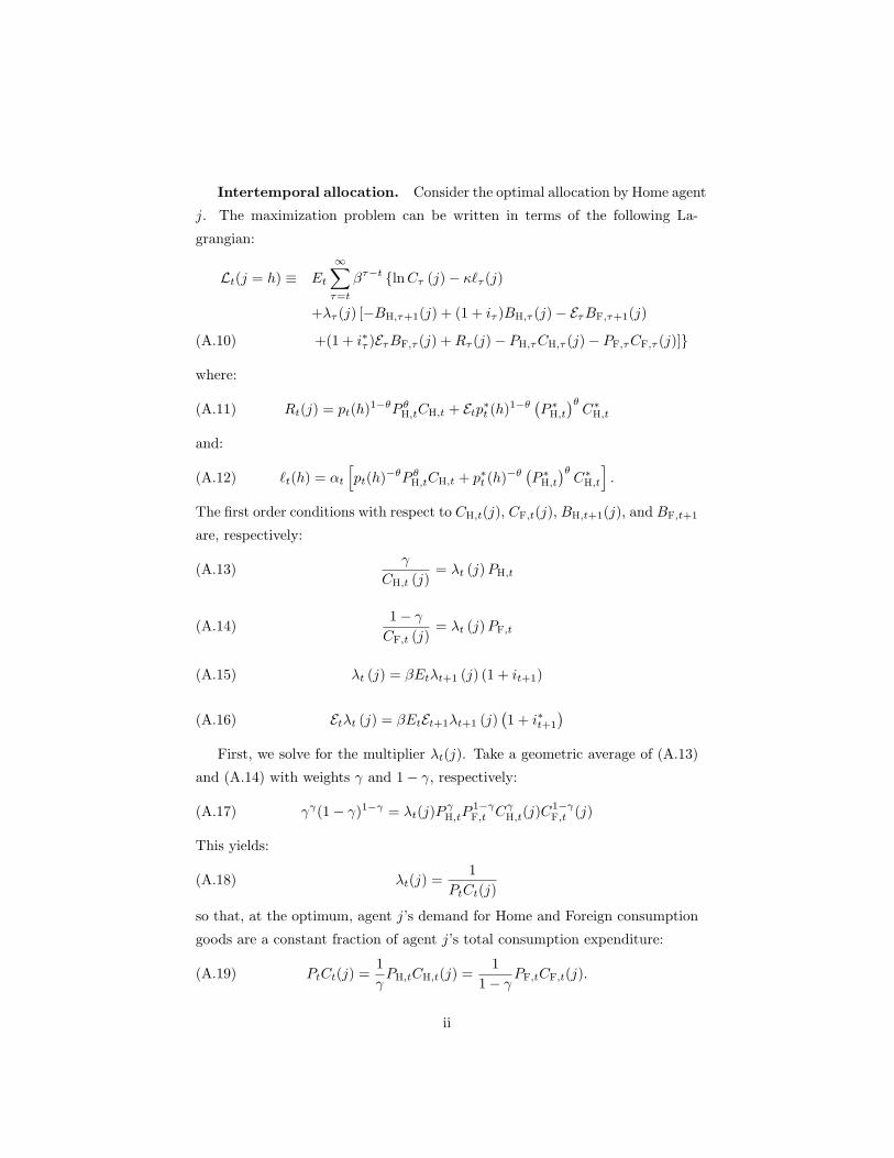
Intertemporal allocation. Consider the optimal allocation by Home agent

j. The maximization problem can be written in terms of the following La-

grangian:

Lt(j = h) ≡ Et

∞∑

τ=t

βτ−t {lnCτ (j)− κ`τ (j)

+λτ (j) [−BH,τ+1(j) + (1 + iτ )BH,τ (j)− EτBF,τ+1(j)

+(1 + i∗τ )EτBF,τ (j) +Rτ (j)− PH,τCH,τ (j)− PF,τCF,τ (j)]}(A.10)

where:

(A.11) Rt(j) = pt(h)1−θP θ

H,tCH,t + Etp∗t (h)1−θ(

P ∗H,t

)θC∗

H,t

and:

(A.12) `t(h) = αt

[

pt(h)−θP θ

H,tCH,t + p∗t (h)−θ

(

P ∗H,t

)θC∗

H,t

]

.

The first order conditions with respect to CH,t(j), CF,t(j), BH,t+1(j), and BF,t+1

are, respectively:

(A.13)γ

CH,t (j)= λt (j)PH,t

(A.14)1− γ

CF,t (j)= λt (j)PF,t

(A.15) λt (j) = βEtλt+1 (j) (1 + it+1)

(A.16) Etλt (j) = βEtEt+1λt+1 (j)(

1 + i∗t+1

)

First, we solve for the multiplier λt(j). Take a geometric average of (A.13)

and (A.14) with weights γ and 1− γ, respectively:

(A.17) γγ(1− γ)1−γ = λt(j)PγH,tP

1−γF,t Cγ

H,t(j)C1−γF,t (j)

This yields:

(A.18) λt(j) =1

PtCt(j)

so that, at the optimum, agent j’s demand for Home and Foreign consumption

goods are a constant fraction of agent j’s total consumption expenditure:

(A.19) PtCt(j) =1

γPH,tCH,t(j) =

1

1− γPF,tCF,t(j).

ii

Using these expressions, it is easy to verify that

(A.20) PtCt(j) = PH,tCH,t(j) + PF,tCF,t(j).

Combining (A.13), (A.14) and (A.15) the intertemporal allocation of con-

sumption is determined according to the Euler equation:

(A.21)1

Ct(j)= β (1 + it+1)Et

(

Pt

Pt+1

1

Ct+1(j)

)

Define now the variable Qt,t+1(j) as:

(A.22) Qt,t+1(j) ≡ βPtCt(j)

Pt+1Ct+1(j)

The previous expression can be interpreted as agent j’s stochastic discount

rate. If markets are complete at the national level (or, if national agents are

symmetric) the stochastic discount rate is identical across individuals so that:

(A.23) Qt,t+1(j) = Qt,t+1.

Comparing (A.22) with (A.15) and (A.16) we obtain:

(A.24) EtQt,t+1 =1

1 + it+1, Et

[

Qt,t+1Et+1

Et

]

=1

1 + i∗t+1

Using (A.24) we can write:

(A.25) BH,t+1(j) = Et {Qt,t+1 [Mt(j) + (1 + it+1)BH,t+1(j)]}

and:

(A.26) EtBF,t+1(j) = Et

{

Qt,t+1(1 + i∗t+1)Et+1BF,t+1(j)}

It follows that the flow budget constraint (7) can also be written as:

(A.27) Et {Qt,t+1Wt+1(j)} ≤ Wt(j) +Rt(j)− PtCt(j)

where Wt+1 is wealth at the beginning of period t+ 1, defined as:

(A.28) Wt+1(j) ≡ (1 + it+1)BH,t+1(j) + (1 + i∗t+1)Et+1BF,t+1(j).

Optimization implies that households exhaust their intertemporal budget

constraint: the flow budget constraint hold as equality and the transversality

condition:

(A.29) limN→∞

Et [Qt,NWN (j)] = 0

is satisfied, where Qt,N ≡∏N

s=t+1 Qs−1,s.

iii

Foreign constraints and optimization conditions. Similar results

characterize the optimization problem of Foreign agent j∗. For convenience, we

report here the key equations. The resource constraint for agent f is:

(A.30)`∗(f)

α∗t

≥ pt(f)−θ∗

P θ∗

F,tCF,t + p∗t (f)−θ∗ (

P ∗F,t

)θ∗

C∗F,t

The flow budget constraint is:

B∗H,t+1(j

∗)

Et+B∗

F,t+1(j∗) ≤ (1 + it)

B∗H,t(j

∗)

Et+(1 + i∗t )B

∗F,t(j

∗) +R∗t (j

∗)− P ∗H,tC

∗H,t(j

∗)− P ∗F,tC

∗F,t(j

∗)(A.31)

and, associating individual j∗ with brand f , sales revenue is:

(A.32) R∗(j∗) =1

Et(pt(f))

1−θ∗P θ∗

F,tCF,t + p∗t (f)1−θ∗ (

P ∗F,t

)θ∗

C∗F,t.

First order conditions yield:

(A.33) P ∗t C

∗t (j

∗) =1

γP ∗H,tC

∗H,t(j

∗) =1

1− γP ∗F,tC

∗F,t(j

∗)

(A.34)1

C∗t (j

∗)= β

(

1 + i∗t+1

)

Et

(

P ∗t

P ∗t+1

1

C∗t+1(j

∗)

)

,

(A.35) Q∗t,t+1(j

∗) = Q∗t,t+1 = β

P ∗t C

∗t (j

∗)

P ∗t+1Ct+1(j∗)

= βλ∗t+1(j

∗)

λ∗t (j

∗),

and:

(A.36) EtQ∗t,t+1 =

1

1 + i∗t+1

, Et

[

Q∗t,t+1

EtEt+1

]

=1

1 + it+1.

Since international bonds are in zero net supply, the following constraints hold:

(A.37)∫ 1

0BH,t(j)dj +

∫ 1

0B∗

H,t(j∗)dj∗ = 0,

∫ 1

0BF,t(j)dj +

∫ 1

0B∗

F,t(j∗)dj∗ = 0

Optimal price setting. Optimal prices in the Home country are derived

as follows. Maximizing the Lagrangian with respect to pt(h) yields:

(A.38) Et−1

[

−κθpt(h)−θ−1P θ

H,tαtCH,t + (θ − 1) pt(h)−θP θ

H,tλt(h)CH,t

]

= 0

iv

or, in a symmetric environment:

(A.39) pt(h) = PH,t =θ

θ − 1

Et−1 [καtCH,t]

Et−1

[

CH,t

PtCt

]

and, using (A.19), we can rewrite the previous expression as (9) in the main

text.

Maximizing the Lagrangian with respect to pt(h) yields:

0 = Et−1

[

−κθp∗t (h)−θpt(h)

−1(

P ∗H,t

)θαtC

∗H,t

+(θ − 1) p∗t (h)1−θEtpt(h)−1

(

P ∗H,t

)θλt(h)C

∗H,t

]

(A.40)

In a symmetric environment with p∗t (h) = P ∗H,t, we can rewrite the above as:

(A.41) 1 =θ κ

θ − 1

Et−1

[

αtC∗H,t

]

Et−1

[

P ∗H,t

EtC∗H,t

PtCt

]

and, using (A.33), we obtain:

(A.42) 1 =θ κ

θ − 1

Et−1

[

αtP ∗t C

∗t

P ∗H,t

]

Et−1

[

EtP ∗t C

∗t

PtCt

]

or:

(A.43) pt (h) =θ

θ − 1

Et−1

[

καtP∗t C

∗t E

η∗

t

]

Et−1

[

EtP ∗t C

∗t

PtCt

]

from which we obtain (11) in the main text using (17) and (18).

Equilibrium. Given initial wealth levels Wt0 and W ∗t0 (symmetric within

each country), and the processes for αt, α∗t , it+1 and i∗t+1 for all t ≥ t0, the fix-

price equilibrium is a set of processes for CH,t, CF,t, Ct, Qt,t+τ , BH,t+1, BF,t+1,

`t, Rt, Wt+1, PH,t, PF,t, Pt, C∗H,t, C

∗F,t, Q

∗t,t+τ , C

∗t , B

∗H,t+1, B

∗F,t+1, `

∗t , R

∗t , W

∗t+1,

P ∗H,t, P

∗F,t, P

∗t , and Et such that, for all t ≥ t0 and τ > t0, (i) Home consumer

optimization conditions (3), (5), (6), (A.19), (A.21), (A.22), (A.24), (A.28), and

their Foreign analogs hold as equalities; (ii) Home firm optimization conditions

v

(9), (11), (4), and their Foreign analogs hold; (iii) the Home transversality con-

dition (A.29) and its Foreign analog hold; (iv) the markets for the international

bonds clear, that is conditions (A.37) hold.

A flex-price equilibrium is similarly defined, after imposing that for all t ≥ t0

Home conditions (9), (11), and their Foreign analogs hold in any state of nature

at time t rather than in expectation at time t− 1.

Equilibrium balanced current account. Aggregating the individual

budget constraints and using the government budget constraint we obtain an

expression for the Home current account:

(A.44) Et {Qt,t+1Wt+1} = Wt +Rt − PtCt

and, by the definition of sales revenue:

(A.45) Rt = PH,tCH,t + EtP ∗H,tC

∗H,t = γ (PtCt + EtP ∗

t C∗t ) .

Assume now that, at time t0, BH,t0 = BF,t0 = 0 so that initial wealth

Wt0 = 0. It is easy to show that, for all t ≥ t0, the equilibrium conditions above

are solved by the allocation:

(A.46) Rt − PtCt = −Et (R∗t − P ∗

t C∗t ) = 0, Wt = −EtW ∗

t = 0 t ≥ t0.

The utility gap. To derive (43) and to show its sign observe that con-

sumption under flexible prices is:

(A.47) Cflext = γ

ΦW

αγt (α

∗t )

1−γ

where

(A.48) ΦW = ΦγΦ∗1−γ , Φ =θ − 1

θ κ, Φ∗ =

θ∗ − 1

θ∗ κ∗ .

vi

Consider now the following steps:

Et−1Wflext − Et−1Wt = Et−1

(

lnCflext − lnCt

)

+ κΦ− κΦ

= Et−1 lnCflex

t

Ct= Et−1 ln

{Et−1 [αtµt]}γ{

Et−1

[

α∗t (µ

∗t )

ηµ1−ηt

]}1−γ

αγt (α

∗t )

1−γµ1−η(1−γ)t (µ∗

t )η(1−γ)

= Et−1

γ lnEt−1 [αtµt]

αtµt

+ (1− γ) lnEt−1

[

α∗t (µ

∗t )

ηµ1−ηt

]

α∗t (µ

∗t )

ηµ1−ηt

= Et−1

[

γ (lnEt−1 [αtµt]− lnαtµt) + (1− γ)(

lnEt−1

[

α∗t (µ

∗t )

ηµ1−ηt

]

− lnα∗t (µ

∗t )

ηµ1−ηt

)]

≥ Et−1

[

γ (Et−1 [lnαtµt]− lnαtµt) + (1− γ)(

Et−1

[

lnα∗t (µ

∗t )

ηµ1−ηt

]

− lnα∗t (µ

∗t )

ηµ1−ηt

)]

= γ (Et−1 lnαtµt − Et−1 lnαtµt) + (1− γ)(

Et−1 lnα∗t (µ

∗t )

ηµ1−ηt − Et−1 lnα

∗t (µ

∗t )

ηµ1−ηt

)

= 0. (A.49)

Optimal monetary rules. Recalling that:

(A.50)∂f [Et−1 (xtµ

πt )]

∂µt

= f ′ [Et−1 (xtµπt )]xtπµ

π−1t ,

the first order condition for maximizing (A.49) with respect to µt is:

(A.51)γαt

Et−1 [αtµt]− γ

µt

+(1− γ) (1− η)α∗

t (µ∗t )

ηµ−ηt

Et−1

[

α∗t (µ

∗t )

ηµ1−ηt

] − (1− γ) (1− η)

µt

= 0

which can be written as (33) in the main text. The other rules are similarly

obtained.

Nominal equilibrium. The optimal monetary rules derived in the main

text do not provide a nominal anchor to pin down nominal expectations. For

instance, recalling the solution for PH,t, we can write the Home country reaction

function (33) in order to emphasize the relation between µt and PH,t:

(A.52) αtµt =

1− η(1− γ)− (1− γ) (1− η)α∗t (µ

∗t )

ηµ1−ηt

Et−1

(

α∗t (µ

∗t )

ηµ1−ηt

)

ΦPH,t

γ

Now, using (19) we obtain ΦPH,t = Et−1αtµt but taking the expectation of

(A.52) we obtain Et−1αtµt = ΦPH,t for any arbitrary choice of PH,t. Similar

considerations hold for (34) and P ∗F,t.

vii

To address this issue, following Woodford [2002], we take µt and µ∗t defined

by the system (33) and (34) and define two rules µt and µ∗t such that:

(A.53) µt = µt

(

PH,t

PH

)δ

µ∗t = µ∗

t

(

P ∗F,t

P ∗F

)δ∗

δ, δ∗ < 0

where δ and δ∗are two negative constants, arbitrarily small, and PH and P ∗F

are the two nominal targets for the Home and Foreign monetary authorities,

respectively. Under the rules above, we obtain:

(A.54) ΦPH,t = Et−1αtµt = Et−1αtµt

(

PH,t

PH

)δ

= γΦ (PH,t)

δ+1

γ(

PH

)δ

solved by PH,t = PH. This implies that, in equilibrium, µt is identical to µt

once we replace PH,t with PH. Similar considerations allow to pin down P ∗F,t =

P ∗F . The government sets a nominal anchor and credibly threatens to tighten

monetary policy if the price of domestic goods deviates from a given target.

Such threat, however, is never implemented in equilibrium.

viii