Embed Size (px)
Citation preview
1
Department of Economics
Issn 1441-5429
Discussion paper 18/09
A Bayesian Approach to Optimum Currency Areas in East Asia
Grace H.Y. Lee1 , M. Azalib
Abstract This paper assesses the empirical desirability of the East Asian economies to an alternative exchange rate arrangement (a monetary union) that can potentially enhance the exchange rate stability and credibility in the region. Specifically, the symmetry in macroeconomic disturbances of the East Asian economies is examined as satisfying one of the preconditions for forming an Optimum Currency Area (OCA). We extend the existing literature by improving the methodology of assessing the symmetry shocks in evaluating the suitability of a common currency area in the East Asian economies employing the Bayesian State-Space Based approach. We consider a model of an economy in which the output is influenced by global, regional and country-specific shocks. The importance of a common regional shock would provide a case for a regional common currency. This model allows us to examine regional and country-specific cycles simultaneously with the world business cycle. The importance of the shocks decomposition is that studying a subset of countries can lead one to believe that observed co-movement is particular to that subset of countries when it in fact is common to a much larger group of countries. In addition, the understanding of the sources of international economic fluctuations is important for making policy decisions. Our findings also indicate that regional factors play a minor role in explaining output variation in both East Asian and the European economies. This implies that while East Asia does not satisfy the OCA criteria (based on the insignificant share of regional common factor), neither does Europe. Keywords: Optimum Currency Area; Business Cycle Synchronisation, Monetary Integration; East Asia JEL codes: E3, F1, F4
1 Corresponding author. e-mail address: [email protected]; phone: +60 3 5514 6000 (Ext -61739); fax: +60 3 5514 6326. Department of Economics, School of Business, Monash University, Jalan Lagoon Selatan, Bandar Sunway, 46150 Selangor, Malaysia b Department of Economics, Faculty of Economics and Management, Universiti Putra Malaysia, 43400 Selangor, Malaysia © 2009 Grace H.Y. Lee and M. Azali All rights reserved. No part of this paper may be reproduced in any form, or stored in a retrieval system, without the prior written permission of the author.

2
1. Introduction
East Asia was late in jumping onto the regionalism bandwagon in comparison with the
European and North American countries. The first Regional Trade Arrangements in East
Asia only existed in 1977 when Association of Southeast Asian Nations (ASEAN)2 reached
an agreement on its Preferential Trading Arrangements. Several further attempts to forge
closer economic integration amongst the East Asian countries during the 1990s were
unsuccessful. Most researchers identified three major reasons for the sudden interest in East
Asia for greater economic integration: (1) the failure of the World Trade Organisation (WTO)
and Asia-Pacific Economic Cooperation (APEC) to make any significant headway on trade
liberalisation. (2) the widening and deepening economic integration in Europe and North
America; and (3) the Asian Financial crisis.
East Asian countries have reassessed their strategies towards further trade liberalisation after
the failure to launch a new round of trade negotiations during the WTO Ministerial Meeting
in Seattle. If the global trading system does not continue to liberalise, the region may be
affected negatively as many of the East Asian countries depend on export to sustain their
economic growth.3 Hence, the perception that a new round of WTO trade negotiations had
failed to materialise due to a lack of enthusiasm and political will in both the US and Europe
has fueled concerns among the East Asian countries about the direction that the global
trading system is heading. In Europe, the European Union (EU) has expanded into Central
and Eastern Europe and will be progressing into greater monetary union. In the United States
(US), North American Free Trade Area (NAFTA) and Latin American countries are heading
towards greater economic integration.
2 Comprising only the founding members: Indonesia, Malaysia, the Philippines, Singapore and Thailand. 3 Bergsten (2000).
3
On the monetary side, the single greatest push for East Asian regionalism was Asian crisis,
sparked in mid-1997 by the devaluation of the Thai baht, and the related global financial
crisis, triggered by the Russian debt default in August 1998, shook the foundations of the
international monetary system. Many East Asian countries felt that they were let down by the
West during the crisis. In their view, western banks and other financial institutions had
created and exacerbated the crisis by pulling out their funds from the region. The leading
financial powers then either declined to take part in the rescue operations (as was the case of
US with Thailand) or built in excessively stringent demands into their financial assistance
programs. At the same time, there was a negative perception among East Asian countries that
the International Monetary Fund (IMF) and the US were dictating their policy responses to
the crisis by controlling their access to funds and private capital markets (Yip, 2001). This
resentment was further fuelled by the widespread view that the IMF’s rescue programs had
worsened the situation for the East Asian economies by pushing them into a deeper economic
recession than was necessary to begin with (Bergsten, 2000). Whether these views were
justified, the East Asian countries have decided that they do not want to be beholden to the
West should a crisis recur in the future (Yip, 2001). The idea of a common currency for APT
became popular after the Asian Financial Crisis 1997. Currency stability was identified as
important to avoiding future financial crises and greater monetary and exchange rate
cooperation is called for in the Chiang Mai Initiative 2000 in Thailand.
After the Chiang Mai Initiative in 2000 that established a regional currency-swap facility, the
idea of a single currency for East Asia was created. There are also efforts beyond the Chiang
Mai Initiative to coordinate macroeconomic and exchange rate policies. An ASEAN Task
Force on ASEAN Currency an Exchange Rate Mechanism was established in March 2001.4
4 The Task Force completed the study in September 2002 and it was presented at the meeting of the ASEAN Central Bank and Finance Deputies in Myanmar in October 2002.
4
In addition, the Kobe Research Project is conducted to provide stimulus to this work through
studies exploring ways and means to improve regional monetary and financial cooperation.
Although the progress and commitment in monetary cooperation in East Asia has been
encouraging, much remains to be accomplished.
Robert Mundell’s OCA theory has been widely used to assess the suitability of the EU to
form a monetary union. Although there has been increasing interest among the researchers to
examine the suitability of East Asian countries for a common regional currency, most of the
related studies have been based primarily on inappropriate econometrics techniques. Simple
correlation between countries is mainly used to measure the degree of shock symmetry in the
OCA literature. The correlation is usually calculated between a country and a chosen anchor
country. Lee et al. (2002) provided some disadvantages of bilateral measures in the
following reasons: (1) the degree of region-wide co-movements, rather than bilateral ones
provides a more appropriate measure since we are interested in the net benefits of adopting a
common monetary policy across economies in the region; (2) the simple correlation does not
offer the sources of the shocks, there may be the third factor such as the world common
shocks that induce a high correlation between countries; (3) there is no single country
plausibly offers a regional anchor.5
Another celebrated technique in OCA literature is Bayoumi’s structural VAR
technique. The first stage of this technique consists of running a national VAR of changes of
output and prices. To identify the coefficients of the structural form, Bayoumi assumed the
orthogonality of supply and demand shocks that only supply shocks are able to affect the
level of output, and that demand shocks are temporary. This approach comes with several
5 In Europe, Germany is generally perceived as the regional anchor. In East Asia, however, there is no country which can play such similar role.
5
caveats. First of all, if the logs of output and prices in quarterly format are cointegrated in
several of the countries of the sample, the coefficients of the VAR are asymptomatically
biased. In addition, as Bayoumi recognises, neither the orthogonality of supply and demand
shocks nor the short duration of demand shocks are uncontestable assumptions. A shock to
terms of trade would affect both aggregate supply and demand. In economies with high
unemployment rates, demand shocks can be expected to have effects that are highly
persistent, if not permanent. Bayoumi and Eichengreen (1994) argued that only supply
shocks are crucial disturbances to which independent monetary policy wishes to respond.
Many researchers see little justification that only supply shocks matter.6 They argue that
there may not be much room left for the policy makers to react to if supply shocks are
permanent shocks. In addition, if demand shocks do not originate from policy
implementations, the monetary policy authority may wish to counteract to these disturbances.
The existing methodologies also fail to recognise the sources of the shocks. For instance, one
does not know whether the economic fluctuations of a country are accounted by the country
specific, regional or the world common factors.
In the business cycle literature, there exists a new strand of methodology that allows
the analysis at a disaggregated level using the Bayesian State-Space Model. However, such
methodology is mainly used to analyse the business cycles in the Western countries. Very
few, to our knowledge, have applied it in the OCA context. We propose to employ this
model which allows us to decompose aggregate shocks into country-specific, regional and
world common business cycles. The importance of studying all three in one model is that
studying a subset of countries can lead one to believe that observed co-movement is
particular to that subset of countries when it in fact is common to a much larger group of
countries. For example, Kose et al. (2003) find that the distinct “European” business cycle in
6 Among others, see Lee et al. (2002).
6
the European countries is due to co-movement common to all countries in the world.
Understanding the sources of international economic fluctuations is important for making
policy decisions. For example, if a country exhibits a large value of the share accounted by
the region common factor, then its business cycle movement is largely synchronised to the
region, indicating that a regional common monetary policy is more effective to respond to
the disturbances. However, if a country possesses a smaller value of the share accounted for
by the region common factor and a larger value of that accounted for by the country-specific
factor, it needs to rely more heavily on its own independent counter-cyclical monetary policy.
Unlike previous studies that examine only the degree of correlations of business cycle among
countries, our study enables us to identify the sources of the economic fluctuations for each
country. As a result, composition of the shocks in East Asia will be identified and
appropriate policy actions can be undertaken accordingly.
2. The Suitability of East Asian Countries for A Common Currency – A Literature
Review
The symmetry of underlying shocks among the East Asian countries provides one of
the preliminary guides in identifying potential members for monetary union. The rationale is
that countries experiencing similar disturbances are likely to respond with similar policies,
thus making them better candidates for forming a monetary union. The estimation of the
incidences of macroeconomic disturbances is inherently empirical. One of the first empirical
papers to have dealt with the issue of macroeconomic disturbances through a statistical
approach is by Bayoumi and Eichengreen (1993, 1994). Applying a variant of the VAR
methodology proposed by Blanchard and Quah (1989), Bayoumi and Eichengreen (1993)
7
assessed the nature of macroeconomic disturbances among different groups of countries.
Bayoumi and Eichengreen (1994) showed that supply shocks are symmetrical among (1)
Japan, South Korea and Taiwan and (2) Hong Kong, Indonesia, Malaysia and Singapore.7
Demand shocks are found to be highly symmetrical for the latter group of countries. Based
on the OCA criterion of symmetry in underlying disturbances, they conclude that these two
groups of countries are likely to form separate OCAs. Their results on the correlation, size
and speed of adjustment to underlying disturbances for Asia are updated in Bayoumi, and
Mauro (1999). 8 It is concluded that aggregate supply disturbances affecting Indonesia,
Malaysia and Singapore are reasonably correlated, while the Philippines and Thailand
experience more idiosyncratic shocks. 9 Their study also reports that, (1) size of the
disturbances experienced by the Asian economies is considerably larger than that of the
equivalent shocks for Europe 10 ; (2) the speed of adjustment in Asia (and ASEAN in
particular) is much more rapid than in Europe. Based on economic criteria, the authors
conclude that ASEAN is less suitable for a currency union than the continental European
countries were in 1987 (a few years before the Maastricht treaty providing a road map for
EMU was signed), although the difference is not very large.11
Using a different methodology from Bayoumi and Eichengreen (1994), Wyplosz
(2001) identifies shocks as the residuals from simple AR(2) regressions of real GDP for the
Asian, European, Australia and New Zealand countries using annual data over the period
1961-1998.12 He finds that shocks in European countries are significantly more correlated
7 Bayoumi and Mauro (1999) argue that aggregate supply disturbances are generally more relevant than aggregate demand disturbances, because aggregate supply disturbances are more related to private sector behaviour rather than the impact of macroeconomic policies. 8 The updated Asian results use data from 1968 to 1998, compared to a sample period of 1969-1989 used in the European results reported. 9 The authors claim that there are parallels with Europe, where the shocks experienced by France and Germany are relatively highly correlated, while those affecting Italy and Spain were more idiosyncratic. 10 This also occurs when the sample period excludes the Asian crisis (1997 and 1998). 11 The authors view firm political commitment as vital in forming a regional currency arrangement. 12 The Asian countries under study include: China, Hong Kong, Indonesia, Japan, Korea, Malaysia, the Philippines, Singapore, Taiwan and Thailand.
8
than shocks in Asian countries.13 It is reported that Korea, Malaysia and Thailand seem to be
more correlated with Japan. As recognized by the author, the difference between his results
and Bayoumi-Eichengreen’s (1994) results can be due to the different methodology or to the
sample period (Bayoumi and Eichengreen’s sample covers from 1972 to 1989).14 Most
empirical analyses based on the theory of optimum currency areas, including those of
Taguchi, and Bayoumi and Eichengreen (1994) and Wyplosz (2001) cited above, have
focused on the costs of monetary integration and studied the correlation of various
macroeconomic variables among the Asian countries. In an effort to combine the various
criteria for a monetary union, Bayoumi and Eichengreen (1999) developed an “OCA index”
that predicts the expected level of exchange rate variability for various Asian countries.15
They derive the index from the results of a cross-sectional regression covering advanced and
East Asian economies that relates observed exchange rate variability to four optimum
currency indicators. The independent variables are: (i) the standard deviation of the
difference in growth rates across the two economies; (ii) the dissimilarity of the composition
of trade; (iii) the level of bilateral trade; and (iv) the size of the two economies. The first two
indicators are proxies for the costs associated with asymmetric shocks, the second two for the
benefits from stabilizing exchange rates with close trading partners and across larger
groupings. Based on the OCA index, the authors report that the following country pairs
achieve scores comparable to those in Western Europe: Singapore-Malaysia, Singapore-
Thailand, Singapore-Hong Kong, Singapore-Taiwan, and Hong Kong-Taiwan.16 However,
Indonesia, South Korea and the Philippines do not rank well, and the Malaysia-Thailand pair
displays a very weak score.
13 Since the author also find that trade integration is deeper in Asia than it is in Europe, it can be concluded that a high degree of trade integration does not translate into strong output correlations. 14 Bayoumi and Eichengreen (1994) find little difference between Europe and Asia for both supply and demand shocks. Besides, different country groupings are identified. 15 The East Asian countries are Japan, Hong Kong, Korea, Singapore, Taiwan, Indonesia, Malaysia, the Philippines and Thailand (covering the sample period from 1976 to 1995). 16 These are the cases where the value of the OCA index approaches Western European levels.

9
These studies are based on historical data before monetary integration. However, the
correlation relations may change after monetary integration as exchange rate fluctuations
among member countries are eliminated. 17 The behaviour of economic agents and the
government will be altered. In a study to examine the possibility of forming a Yen bloc in
Asia, Kwan (1998) stresses the importance of using correlation of economic structures and of
policy objectives as OCA criteria since they are less dependent on the exchange-rate system.
He quantifies the degree of similarity in the economic structures of two countries in terms of
the correlation coefficient between vectors showing their respective share composition of
trade (imports and exports) classified by product18. Such correlation coefficient can also be
used as an indicator of the degree of competition (or complementarity) in the trade structures
of two countries. It is found that countries with similar per capita incomes tend to have
similar trade structures since the latter is closely related to the level of economic
development. Kwan finds that trade structures in Asian countries are less similar than the
trade structures of West European countries.19 By comparing inflation rates (to examine the
similarity of policy objectives among nations), the author finds that East Asia qualifies as an
optimum currency area as much as West Europe 20 , 21 . Therefore, by the “similarity in
inflation rate” criterion, low-inflation countries such as Singapore, Taiwan, Malaysia,
Thailand, and South Korea, which also belong to the higher income group, are more
appropriate candidates for forming a yen bloc.
17 Kwan (1998) illustrates this by noting the relations between Japan and South Korea. With South Korea belonging to the dollar bloc, fluctuations in the yen-dollar rate affect Korea and Japan asymmetrically. An appreciation of the yen, for example, will increase the inflation and economic growth for South Korea but reducing the inflation and economic growth for Japan. If Japan and South Korea form a monetary union, however, such asymmetric shock would be eliminated and the correlation of economic growth rates and of inflation rates between the two countries would increase. 18 The bilateral correlation coefficients are calculated based on the three-category classification for exports and imports, namely primary commodities, machinery, other manufacturers. 19 The 45 correlation coefficients for the 10 Asian countries (Korea, Taiwan, HK, Singapore, Indonesia, Malaysia, Philippines, Thailand, China and Japan) averaged 0.28 while the 55 correlation coefficients for the 11 West European countries (U.K., France, Italy, Belgium, Netherlands, Denmark, Ireland, Spain, Portugal and Greece) averaged 0.52. 20 Kwan (1998) reports that between 1982 and 1996, the inflation rate of the Asian countries averaged 5.8% a year, marginally lower than the 6.1% annual average for the West European countries. The standard deviation showing the dispersion of inflation rates among countries is also smaller for East Asia than for West Europe. 21 The author also notes that inflation rates among the West European countries have shown signs of convergence in recent years as they move closer to a monetary union.

10
3. Methodology
The econometric model employed here follows the dynamic unobserved factor model
in Kose et al. 2003), which is an extension of the single dynamic unobserved factor model in
Otrok and Whiteman (1998). The world economy consists of many different regions and
each region consists of many different countries. The movement of an aggregate output in
each country i is decomposed into three different components: (i) the world common
component, (ii) the region common component and (iii) the country-specific component.
Every country in the world is influenced by the world common, while the region common
component influences only the countries belonging to the same region. The influence of
country-specific component is restricted to the specific country. For example, the output of
Malaysia fluctuates due to shocks to the world economy, shocks to the East Asian region or
Malaysia-specific shocks.
We should recognise that it is not a threshold question that East Asia’s business cycle
synchronisation must pass a certain value in order to satisfy the OCA criteria. In fact, there
are no exact empirical standards set for the OCA criteria and researchers can only make their
own judgments based on the empirical results. The Euro Area, the first region in the world to
adopt a single currency, should be used as the benchmark for any regions who are interested
to form a monetary union. In this paper, the benchmarks of the comparison are the European
Union and the North American countries.22
In our model, there are K dynamic, unobserved factors thought to characterise the
temporal comovement in the cross-country panel of economic time series. Let Yi,t denote a
22 Refer to Appendix for a list of the countries in these regions.
11
measure of observable aggregate output at time t for country i, N denote the number of
countries, M the number of time series per country, and T the length of the time series.
The output series for each country is decomposed into three separate components:
ε tiNtni
Rtri
Wtwiiti YbYbYbaY ,, ++++= (1)
E εi,t εj,t-s = 0 for i ≠ j
Let YWt (world common factor) be an unobservable component of world economic activity
common to all the countries; Y Rt (region common factor) be an unobservable component
common to each country belonging to the same region R and Y Nt be an unobservable
component of country specific factors. There are three regions considered: East Asia, Europe
and North America areas. If R = 1, that country belongs to East Asia, if R = 2, it belongs to
the Europe, and if R = 3, it belongs to North America.
The coefficients, bwi, bri and bni are the impact coefficients on factorsYWt , Y R
t andY N
t ,
reflecting the degree to which variation in yi can be explained by each factor. The impact
coefficients are allowed to differ across countries since the world common and the region
common factors have different influences on each country. There are M×N time series to be
“explained” by the (many fewer) N+R+1 factors. The “unexplained” idiosyncratic errors εi,t
are assumed to be normally distributed, but may be serially correlated and are modeled as pi -
order autoregressions:
( ) uL titii ,,ø =ε (2)
or ( ) LLLLii
i
ppi,2i,1i, ø-...-ø-ø-1ø =
is a polynomial in the lag operator L; Eui,t uj,t-s = σ2i for i = j and s = 0, 0 otherwise.
The evolution of the unobserved factors is likewise governed by an autoregression of qi -
order with normal errors:
12
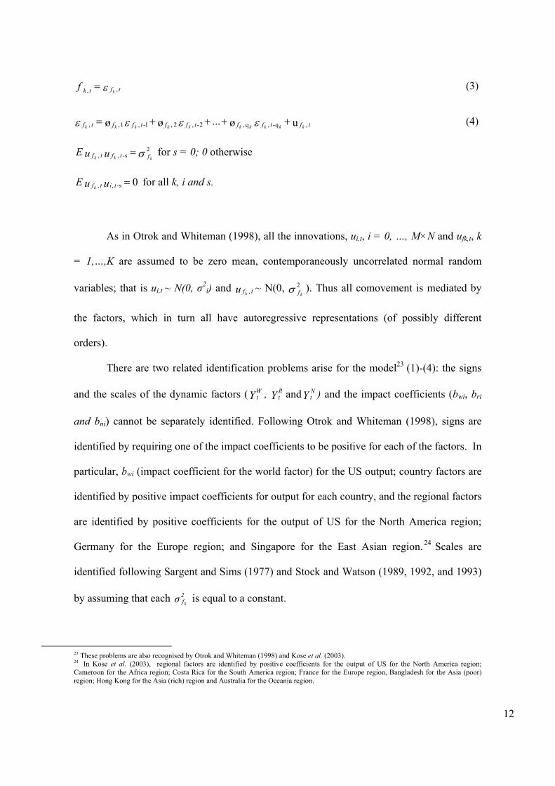
ε tftk kf ,, = (3)
uø...øø ,q- ,q ,2- ,2 ,1- ,1 ,, tftfftfftfftf kkkkkkkkkk++++= εεεε (4)
σ 2s-,, kkk ftftf uuE = for s = 0; 0 otherwise
0s-,, =uuE titfk for all k, i and s.
As in Otrok and Whiteman (1998), all the innovations, ui,t, i = 0, …, M×N and ufk,t, k
= 1,…,K are assumed to be zero mean, contemporaneously uncorrelated normal random
variables; that is ui,t ~ N(0, σ2i) and u tfk , ~ N(0, σ 2
kf ). Thus all comovement is mediated by
the factors, which in turn all have autoregressive representations (of possibly different
orders).
There are two related identification problems arise for the model23 (1)-(4): the signs
and the scales of the dynamic factors (YWt , Y R
t andY N
t ) and the impact coefficients (bwi, bri
and bni) cannot be separately identified. Following Otrok and Whiteman (1998), signs are
identified by requiring one of the impact coefficients to be positive for each of the factors. In
particular, bwi (impact coefficient for the world factor) for the US output; country factors are
identified by positive impact coefficients for output for each country, and the regional factors
are identified by positive coefficients for the output of US for the North America region;
Germany for the Europe region; and Singapore for the East Asian region.24 Scales are
identified following Sargent and Sims (1977) and Stock and Watson (1989, 1992, and 1993)
by assuming that each σ 2fk
is equal to a constant.
23 These problems are also recognised by Otrok and Whiteman (1998) and Kose et al. (2003). 24 In Kose et al. (2003), regional factors are identified by positive coefficients for the output of US for the North America region; Cameroon for the Africa region; Costa Rica for the South America region; France for the Europe region, Bangladesh for the Asia (poor) region; Hong Kong for the Asia (rich) region and Australia for the Oceania region.
13
However, the dynamic factors ( YWt , Y R
t and Y N
t ) are unobservable, traditional
methods cannot be employed and special methods must be used to estimate the model.
Gregory et al. (1997) follow Stock and Watson (1989, 1992 and 1993), using classical
statistical techniques employing the Kalman filter for estimation of the model parameters,
and the Kalman smoother to extract an estimate of the unobserved factor. They treat a related
model as an observer system. Otrok and Whiteman (1998) used an alternative model based
on a recent development in the Bayesian literature on missing data problems called “data
augmentation” (Tanner and Wong, 1987).
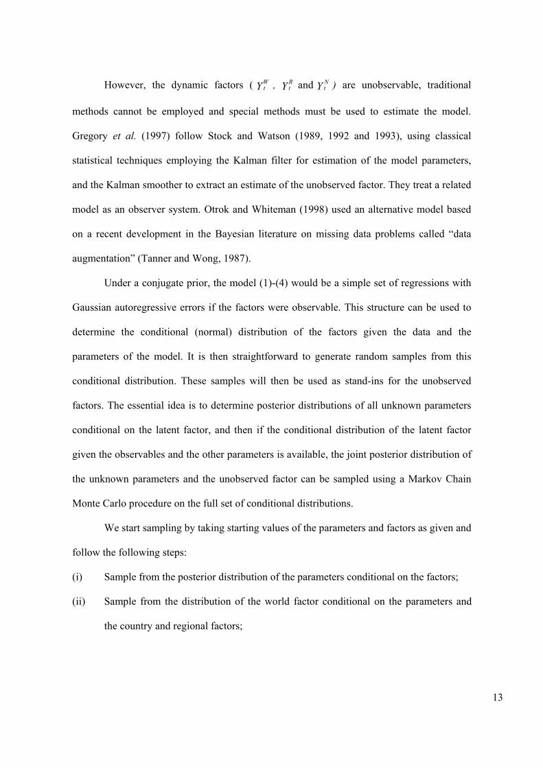
Under a conjugate prior, the model (1)-(4) would be a simple set of regressions with
Gaussian autoregressive errors if the factors were observable. This structure can be used to
determine the conditional (normal) distribution of the factors given the data and the
parameters of the model. It is then straightforward to generate random samples from this
conditional distribution. These samples will then be used as stand-ins for the unobserved
factors. The essential idea is to determine posterior distributions of all unknown parameters
conditional on the latent factor, and then if the conditional distribution of the latent factor
given the observables and the other parameters is available, the joint posterior distribution of
the unknown parameters and the unobserved factor can be sampled using a Markov Chain
Monte Carlo procedure on the full set of conditional distributions.
We start sampling by taking starting values of the parameters and factors as given and
follow the following steps:
(i) Sample from the posterior distribution of the parameters conditional on the factors;
(ii) Sample from the distribution of the world factor conditional on the parameters and
the country and regional factors;
14
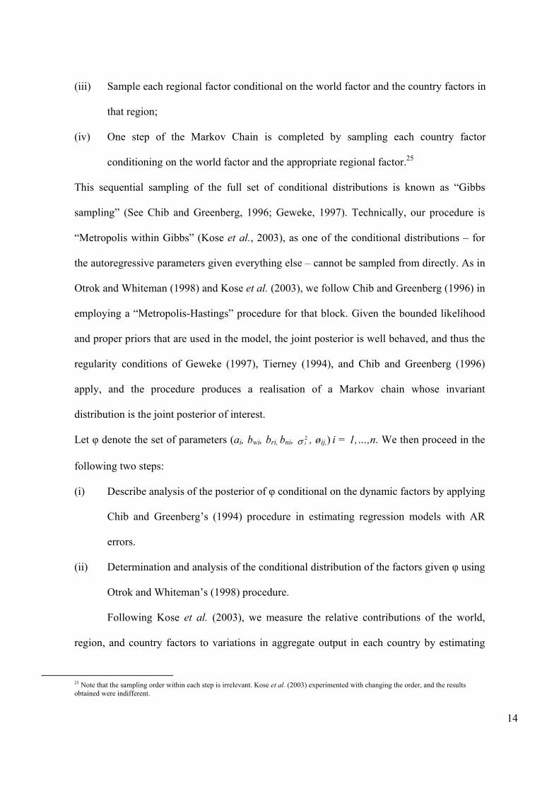
(iii) Sample each regional factor conditional on the world factor and the country factors in
that region;
(iv) One step of the Markov Chain is completed by sampling each country factor
conditioning on the world factor and the appropriate regional factor.25
This sequential sampling of the full set of conditional distributions is known as “Gibbs
sampling” (See Chib and Greenberg, 1996; Geweke, 1997). Technically, our procedure is
“Metropolis within Gibbs” (Kose et al., 2003), as one of the conditional distributions – for
the autoregressive parameters given everything else – cannot be sampled from directly. As in
Otrok and Whiteman (1998) and Kose et al. (2003), we follow Chib and Greenberg (1996) in
employing a “Metropolis-Hastings” procedure for that block. Given the bounded likelihood
and proper priors that are used in the model, the joint posterior is well behaved, and thus the
regularity conditions of Geweke (1997), Tierney (1994), and Chib and Greenberg (1996)
apply, and the procedure produces a realisation of a Markov chain whose invariant
distribution is the joint posterior of interest.
Let φ denote the set of parameters (ai, bwi, bri, bni, σ 2i , øij,) i = 1,…,n. We then proceed in the
following two steps:
(i) Describe analysis of the posterior of φ conditional on the dynamic factors by applying
Chib and Greenberg’s (1994) procedure in estimating regression models with AR
errors.
(ii) Determination and analysis of the conditional distribution of the factors given φ using
Otrok and Whiteman’s (1998) procedure.
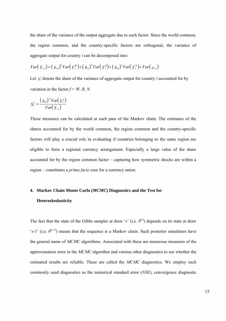
Following Kose et al. (2003), we measure the relative contributions of the world,
region, and country factors to variations in aggregate output in each country by estimating
25 Note that the sampling order within each step is irrelevant. Kose et al. (2003) experimented with changing the order, and the results obtained were indifferent.
15
the share of the variance of the output aggregate due to each factor. Since the world common,
the region common, and the country-specific factors are orthogonal, the variance of
aggregate output for country i can be decomposed into:
( ) ( ) ( ) ( ) ( ) ( ) ( ) ( )ε tiNtni
Rtri
Wtwiti VarYVarbYVarbYVarbYVar ,
222, +++=
Let S fi denote the share of the variance of aggregate output for country i accounted for by
variation in the factor f = W, R, N.
( ) ( )( )YVar
YVarbS
ti
ftfif
i,
2
=
These measures can be calculated at each pass of the Markov chain. The estimates of the
shares accounted for by the world common, the region common and the country-specific
factors will play a crucial role in evaluating if countries belonging to the same region are
eligible to form a regional currency arrangement. Especially a large value of the share
accounted for by the region common factor – capturing how symmetric shocks are within a
region – constitutes a prima facie case for a currency union.
4. Markov Chain Monte Carlo (MCMC) Diagnostics and the Test for
Heteroskedasticity
The fact that the state of the Gibbs sampler at draw ‘s’ (i.e. θ(s)) depends on its state at draw
‘s-1’ (i.e. θ(s-1)) means that the sequence is a Markov chain. Such posterior simulators have
the general name of MCMC algorithms. Associated with these are numerous measures of the
approximation error in the MCMC algorithm and various other diagnostics to see whether the
estimated results are reliable. These are called the MCMC diagnostics. We employ such
commonly used diagnostics as the numerical standard error (NSE), convergence diagnostic

16
(CD), estimated potential scale reduction and the highest potential density intervals (HPDI).
In practice, there are numerous computer programs for these diagnostics available over the
web. We employ James LeSage’s Econometrics Toolbox (LeSage, 1999) using MATLAB.26
We have passed all the above mentioned convergence diagnostics, confirming that the
posterior simulators are working well and the number of draws is sufficient to achieve the
desired degree of accuracy.27 The results of these MCMC diagnostics are reported from
Table 1 to Table 7.
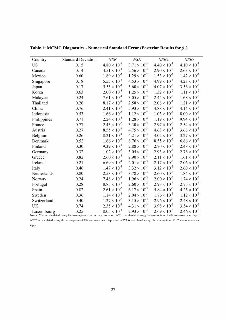
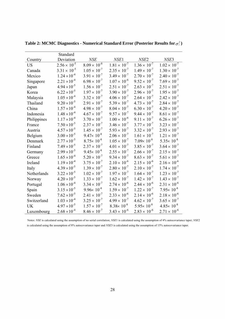
4.1 Numerical Standard Error (NSE)
The NSEs columns presented in Table 4.1, 4.2 and 4.3 represent the approximation of E( β i | y),
E(σ 2i | y) and E(φ i | y) for i =1, 2,…, 28 (denoting the number of countries in this study).
[Insert Table 1 here]
[Insert Table 2 here]
[Insert Table 3 here]
These tables present the results of posterior means, standard deviation and the NSEs based on
the assumptions of no serial correlation, 4% autocovariance taper, 8% autocovariance taper
and 15% autocovariance taper. For instance, the NSE relating to the estimation of E( β1 | y) is
4.80 × 10⁻⁴, E(σ 21 | y) is 8.09 × 10⁻⁸ and E(φ1 | y) is 9.19 × 10⁻⁴. The results indicate that we are
achieving reasonably precise estimates. 26 Other available programs for the same purpose include BUGS and BACC. 27 The MCMC results are available upon request.
17
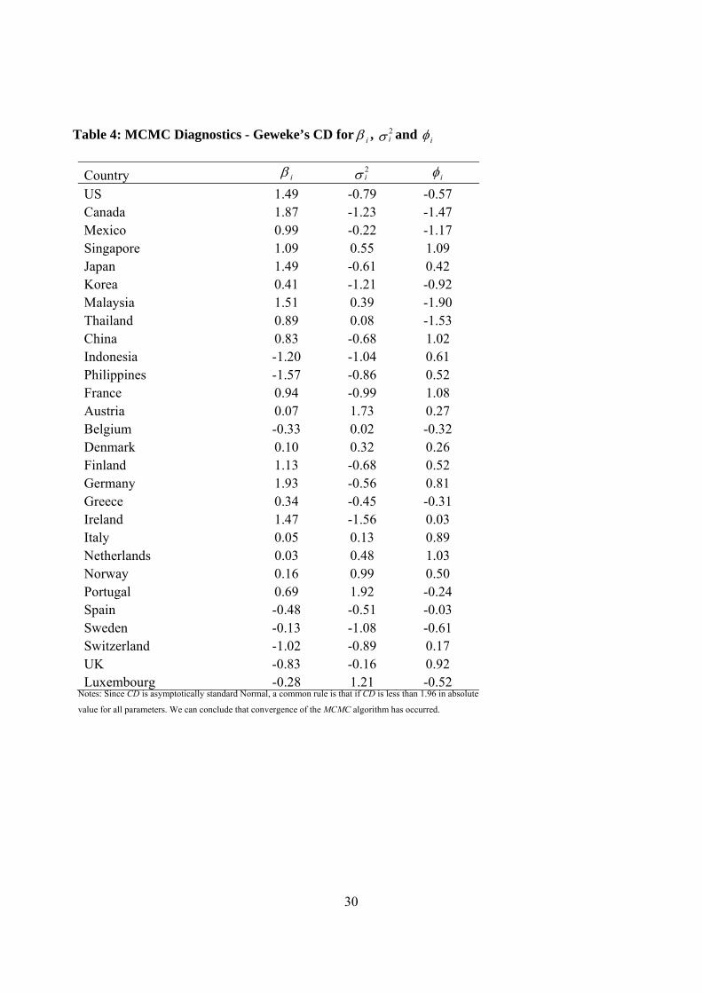
4.2 Convergence Diagnostic (CD)
As pointed out by Koop (2003), the Gibbs sampler may yield misleading results if the initial
replication is extremely far away from the region of the parameter space where most of the
posterior probability lies. The CD will detect this problem as the draws are divided into 3 sets
and the estimation based on the first half of the draws should be essentially the same as the
estimate based on the last half. We follow the standard practice of setting SA = 0.1S1, SB =
0.5S1 and SC = 0.4S1. The reported results are based on S1=100,000; therefore SA=10,000,
SB=50,000 and Sc=40,000. Since CD is asymptotically standard Normal, a common rule is that
if CD is less than 1.96 in absolute value for all parameters, we can conclude that convergence
of the MCMC algorithm has occurred.
[Insert Table 4 here]
Table 4 shows the Geweke’s CD for all the parameters β i , σ2i andφ i . The figures shown in the
table compares the estimation based on the first 10,000 replications (after the burn-in
replications) to that based on the last 40,000 replications. It is evident that CD is less than 1.96
in absolute value for all parameters in Table 4. We can therefore conclude that the initial
condition has vanished and an adequate number of draws have been taken. In other words, the
MCMC algorithm has converged.
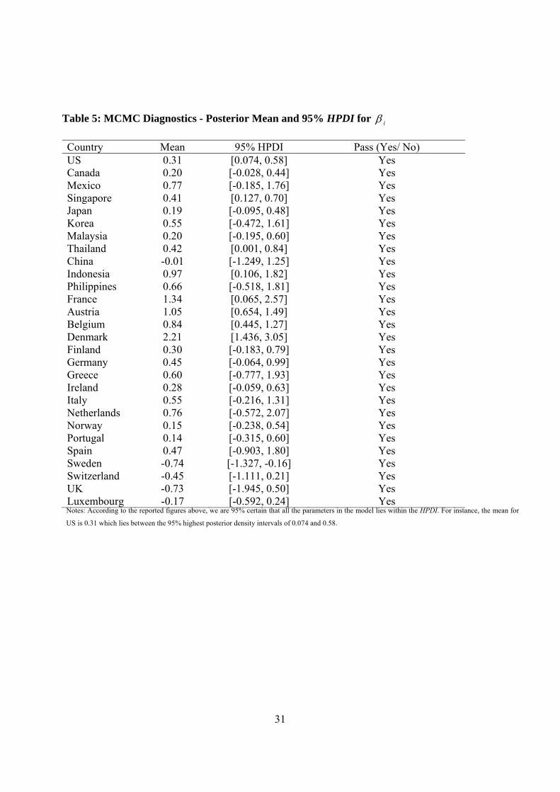
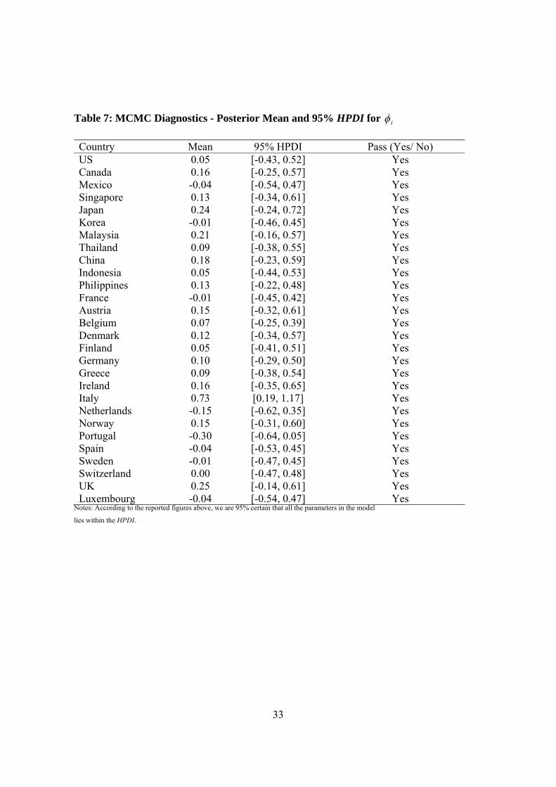
4.3 Highest Posterior Density Intervals (HPDI)
18
This section reports the posterior mean and the 95% HPDI of β i , σ2i and φ i in Table 5, 6 and
7 respectively.
[Insert Table 5 here]
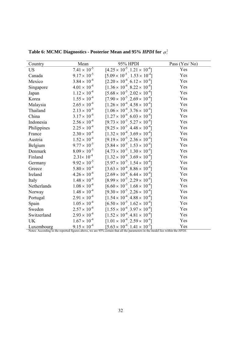
[Insert Table 6 here]
[Insert Table 7 here]
According to the reported figures in Table 5, 6 and 7, we are 95% certain that all the
parameters in the model ( β i , σ2i andφ i ) lies within the HPDI. For instance, the mean for β1 is
0.31 which lies between the 95% highest posterior density intervals of 0.074 and 0.58.
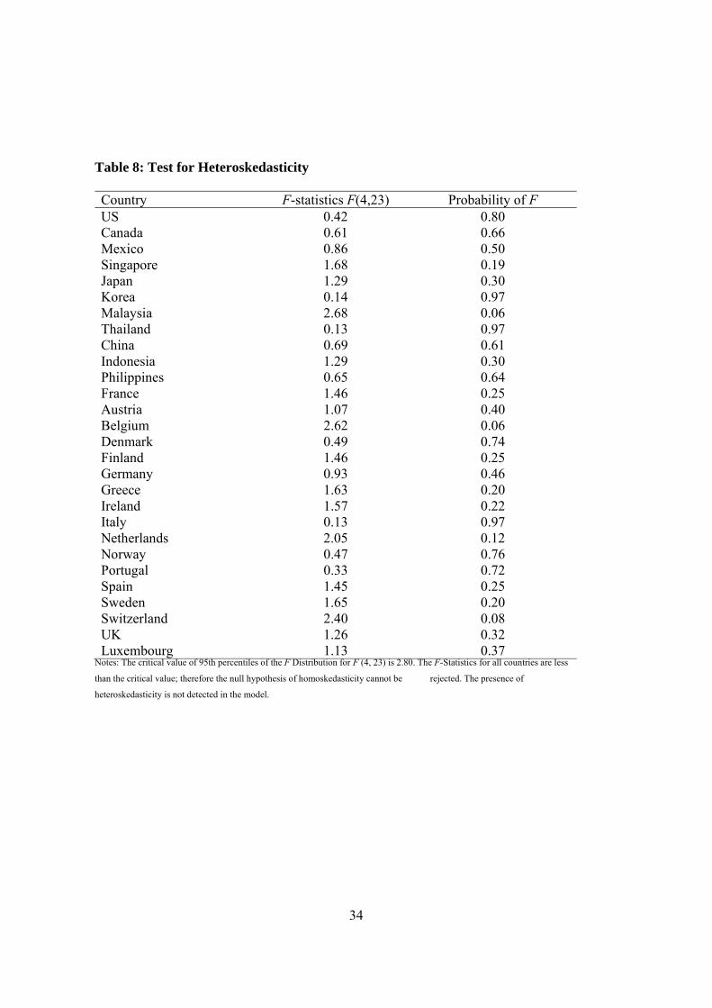
4.4 Test for Heteroscedasticity
The test for heteroscedasticity is being conducted to examine if the error variances
differ across observations. The results presented in Table 8 show that the presence of
heteroscedasticity is not detected in the model.28
[Insert Table 8 here]
5. Results and Estimation
This study examines eight East Asian countries, namely ASEAN 5 – Indonesia,
Malaysia, the Philippines, Singapore and Thailand – and China, Japan and Korea.29 The list
28 Among others, the Bayesian model with heteroscedasticity can be estimated using the GAUSS program. The Gauss codes are provided in Luc Bauwens’ website that accompanied the book Bauwens et al. (1999).

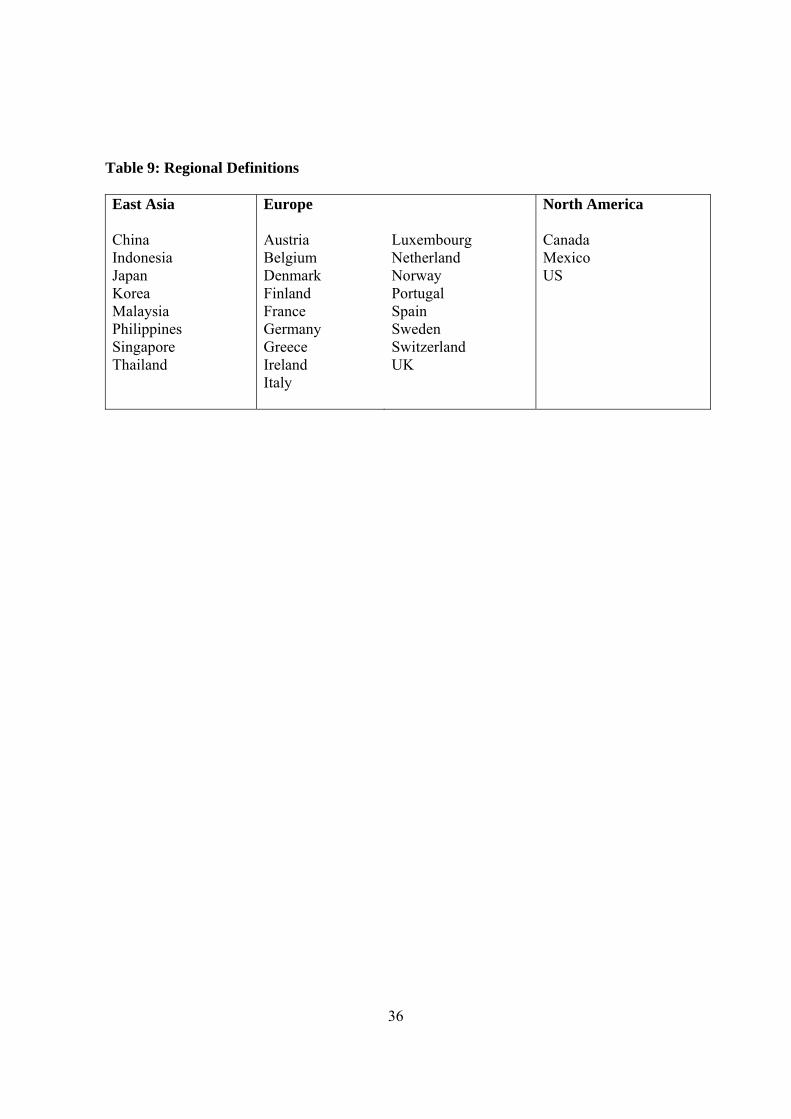
19
of 17 European and 3 North American countries included in the study is provided in the
Appendix (Table 9).
[Insert Table 9 here]
The data used in this paper are drawn from the Penn World Table, the sample period
is from 1970 to 2000.30 Output is measured by the log of real GDP growth. Gauss program is
used in the estimation. It can be shown that the accuracy of the model estimation gets better
and better as the number of replications is increased. In order to get highly accurate estimates,
we set S = 100,000 and discard an initial 10,000 burn-in replications.
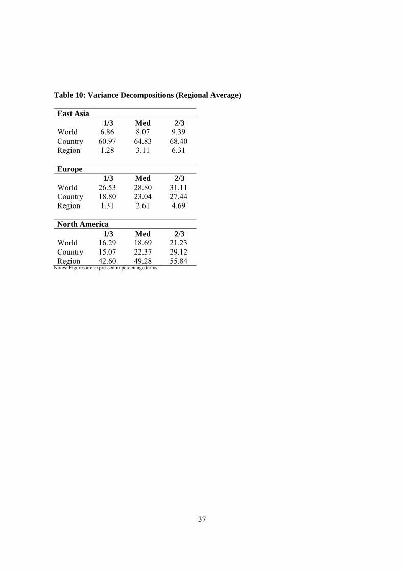
We report the variance shares (medians, 33% and 67% quantiles of posterior)
attributable to the world, regional and country factors for East Asia, Europe and North
America in Tables 10.31
[Insert Table 10 here]
5.1 East Asia
[Insert Table 11 here]
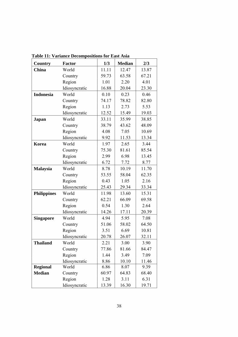
Table 11 demonstrates variance decompositions for the East Asian countries. The
country-specific factors capture the greatest share of output fluctuations in the region,
explaining about 65% of output volatility. However, the country-specific factors share of
29 The new ASEAN members include Cambodia, Laos, Myanmar and Vietnam are excluded in the study as the stages of development in these countries are very much different from the rest of the East Asian countries. Williamson (1999), for example, omits the new members of ASEAN, limiting the heterogeneity of the countries adopting a common basket peg. We lack data on Brunei.
30 It is our intention to examine the business cycle synchronisation for the European countries before the adoption of Euro. 31 Figures for idiosyncratic factors are not reported here. Since there are only 28 countries in our model, the unexplained output movement (which falls under idiosyncratic factors) is expected to be large. Another explanation for the large role of the idiosyncratic factor is measurement error and this is especially true for developing or less developed economies.
20
output volatility ranges widely across the East Asian region, from a low of 43.62% in Japan
to a high of 81.61% and 81.66% in Korea and Thailand respectively using the median
quantile.
The world and region factors, on the other hand, play a relatively modest role in
accounting for the economic activities in these countries. For the median country, only 8% of
the output variation is due to the world factor and only about 3% of the output variation is
due to the East Asian regional factor. The region factor is largest for the most developed
economies in the region, namely, Japan, Korea and Singapore. The region factor accounts for
about 7% of output variation in these countries. In fact, the world factor share of output
volatility also ranges widely across the region from a low of less than 1% in Indonesia to a
high of more than 36% in Japan. This result is consistent with that of Kose et al. (2003) who
found Japan’s world factor to be important.
5.2 Europe
[Insert Table 12 here]
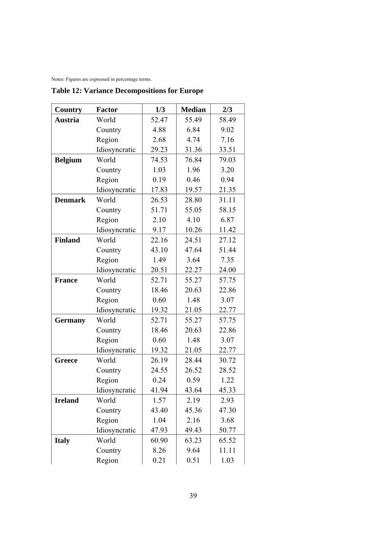
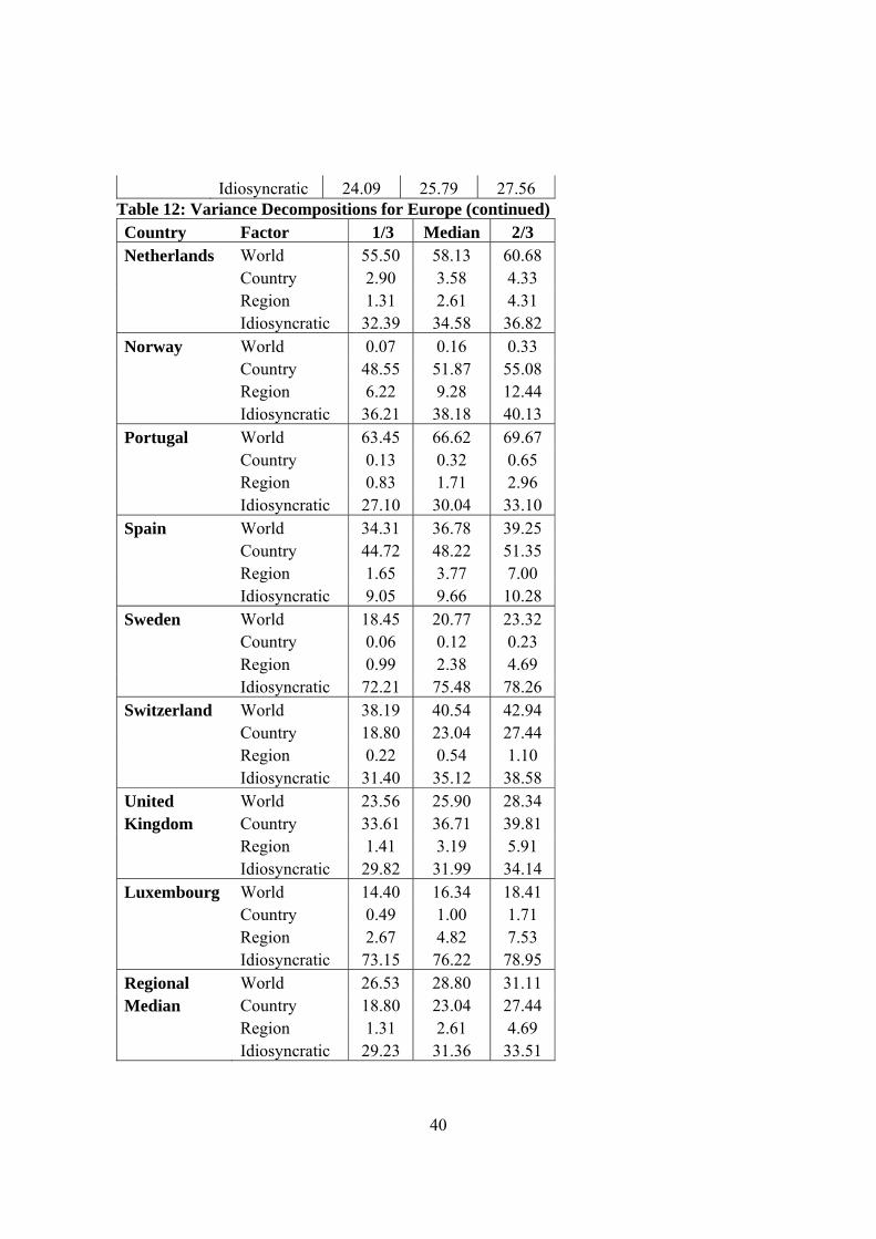
Table 12 demonstrates variance decompositions for the European countries. The
world factor explains more than 28% of the output fluctuations in these economies. However,
the world factor share of output fluctuations varies widely across these countries, ranging
from a low of less than 2.5% in Ireland and Norway to a high of 77% in Belgium.
Though less important than in East Asia, the country-specific factor explains a
noticeable 23% of output volatility in Europe. The country-specific factors, however, are
more important for some countries in the region than others. For instance, country-specific
21
factor account for more than 50% of output volatility in Denmark and Norway and it
accounts for more than 40% of output volatility in Finland, France, Ireland and Spain.
However, the country-specific factor only accounts for less than 5% of output volatility in
Belgium, Netherlands, Portugal, Sweden and Luxembourg.
The European regional factor, however, plays a relatively minor role in accounting
for the economic activity in these countries: it accounts for about 5% of output volatility in
Austria and Luxembourg, and about 9% of output volatility in Norway. The regional factors
in the rest of the European countries are insignificant.
5.3 North America
[Insert Table 13 here]
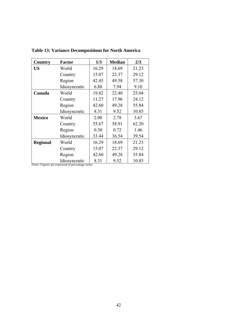
Table 13 presents the variance decompositions for the North America. It is evident
that the regional factor explains the majority of volatility in output, accounting for about 50%
of output volatility in US and Canada. The results for Mexico however, show a different
trend with the country factor explaining the majority of the output fluctuation, the regional
factor only explains less than 1% of output fluctuation.
22
6. Conclusion
The empirical results suggest that the country-specific factors explain the majority of
output volatility in the East Asian economies. Most of the East Asian economies exhibit little
co- movement with the rest of the world compared with Europe and North America. The
world factor explains a noticeable fraction of aggregate output volatility in the Europe and
North American economies. Our findings also indicate that regional factors play a minor role
in explaining output variation in both East Asia and the European economies. This implies
that while East Asia does not satisfy the OCA criteria (based on the insignificant share of
regional common factor), neither does Europe. The regional factor seems to be playing its
most important role in the North American region.
In economic discussions, the loss of the exchange rate instrument was often put
forward as the main argument against monetary union. Our results imply that it could be
costly to renounce individual currencies to advance into a currency union in East Asia as the
output variations explained by country-specific factors is significant. For the time being,
there may not exist scope for East Asia to form a monetary union. Although we do not find
the evidence of a European cycle which provides a case for a regional common currency, the
output in most European countries fluctuates due to shocks to the world economy.
Critics may rightly charge that East Asia lacks the fundamental conditions necessary
for monetary union. However, it is important to note that the perspective of those interested
in pursuing the idea. Proponents acknowledge that monetary union is impossible in the short
term but consider it feasible in the long term. To realise the goal in the future, leaders must
begin laying the groundwork today. More studies need to be done to shed light on the
23
prospect of a single currency for East Asia. Policy makers who are interested to pursue the
idea of a single currency for East Asia must conduct every possible study related to this issue.
7. Limitation of the Study and Future Studies
The results of our study will only shed light on suitability of East Asia to form a
single currency based on how far we are compared to the Euro Area in terms of the business
cycle synchronisation. Of course, many more studies that are outside the scope of this paper
need to be done to examine the suitability of East Asia to form a single currency. Political
will, for instance, is one of the key determinants of whether or not a country would join the
monetary union.
A country’s suitability to form a monetary union depends, inter alia, on their trade
integration and the extent to which its business cycles are correlated. However, studies have
shown that both international trade patterns and international business cycle correlations are
endogenous. A region’s business cycle may become more synchronised after a monetary
union is formed. This can be explained by the increased intra-regional trade (after the
elimination of exchange fluctuations among the countries in the region) that potentially
increases the business cycle synchronisation. It follows that countries are more likely to
satisfy the criteria for entry into a currency union after taking steps toward economic
integration than before. If such hypothesis is empirically verified, policy makers have little to
worry about the region being unsynchronised in their business cycles as the business cycles
will become more synchronised after the monetary union is formed. From a theoretical
viewpoint, the effect of increased trade integration on the cross-country correlation of
business cycle activity is ambiguous. Empirical evidence has shown mixed results. Therefore,

24
it is imperative to investigate the relationship between business cycle synchronisation and
trade integration while examining the suitability of a region to form an OCA.

25
References Bauwens, L., Lubrano, M. and Richard, J.-F., 1999. Bayesian Inference in Dynamic
Econometric Models. Oxford: Oxford University Press. Bayoumi, T., Eichengreen, B., 1993. Shocking Aspects of European Monetary Unification.
In: Torres, F., Giavazzi, F. (Eds.). Adjustment and Growth in the European Monetary Union, Cambridge: Cambridge University Press.
Bayoumi, T., Eichengreen, B., 1994. One Money or Many? Analyzing the Prospects for Monetary Unification in Various Parts of the World. Princeton Studies in International Finance 76.
Bayoumi, T., Eichengreen, B., 1999. Is Asia an Optimum Currency Area? Can It Become One? Regional, Global and Historical Perspectives on Asian Monetary Relations. In: Collignon, S., Pisani-Ferry, J., Park, Y.C. (Eds.). Exchange Rate Policies in Emerging Asian Countries, London: Routledge, pp. 347-66.
Bayoumi, T. and Mauro, P., 1999. The Suitability of ASEAN for a Regional Currency Arrangement. International Monetary Fund Working Paper no. WP/99/162. Bergsten, F., 2000. Towards a Tripartite World. The Economist, 15 July, 20-22. Blanchard, O., Quah, D., 1989. The Dynamic Effects of Aggregate Demand and Supply
Disturbances. American Economic Review 79, 655-73. Chib, S., Greenberg, E., 1994. Bayes Inference in Regression Models with ARMA (p, q)
Errors. Journal of Econometrics 64, 183-206. Chib, S., Greenberg, E., 1996. Markov Chain Monte Carlo Simulation Methods in
Econometrics. Econometric Theory 12, 409-431. Geweke, J., 1997. Posterior Simulators in Econometrics. In: Kreps, D. and Wallis, K.F.
(Eds.). Advances in Economics and Econometrics: Theory and Applications, 3, Cambridge: Cambridge University Press, pp. 128-65.
Gregory, A.W., Head A.C. and Raynauld, J., 1997. Measuring World Business Cycles. International Economic Review 38(3), 677-701. Koop, Gary., 2003. Bayesian Econometrics. John Wiley & Sons. Kose, M.A., Otrok, C., Whiteman, C.H., 2003. International Business Cycles: World, Region,
and Country-Specific Factors. American Economic Review 93(40), 1216-39. Kwan, C.H., 1998. The Theory of Optimum Currency Areas and the Possibility of Forming a
Yen Bloc in Asia. Journal of Asian Economics 9(4). Lee, J., Park, Y.C., Shin, K., 2002. A Currency Union in East Asia. Study on Monetary and
Financial Cooperation in East Asia, prepared for the Asian Development Bank, Preliminary draft.
LeSage, J., 1999. Applied Econometrics Using MATLAB. Available at http://www.spatial- econometrics.com/.
Otrok, C. and Whiteman, C.H., 1998. Bayesian Leading Indicators: Measuring and Predicting Economic Conditions in Iowa. International Economic Review 39(4), 997- 1014.
26
Sargent, T.J., Sims, C., 1977. Business Cycle Modeling Without Pretending to Have Too Much a Priori Theory. In: Sims, C. (Ed.). New Methods of Business Cycle Research, Minneapolis: Federal Reserve Bank of Minneapolis.
Stock, J.H., Watson, M.W., 1989. New Indexes of Coincident and Leading Economic Indicators. In: Blanchard, O., Fischer, S. (Eds.). NBER Macroeconomic Annual, Cambridge: MIT Press, 351-94.
Stock, J.H., Watson, M.W., 1992. A Procedure for Predicting Recessions with Leading Indicators: Econometric Issues and Recent Performance. Federal Reserve Bank of Chicago Working Paper no. WP-92-7, Federal Reserve Bank of Chicago.
Stock, J.H., Watson, M.W., 1993. A Procedure for Predicting Recessions with Leading Indicators: Econometric Issues and Recent Experience. In Business Cycles, Indicators and Forecasting, J. H. Stock and M. W. Watson, Chicago: University of Chicago Press for NBER, 255-84.
Taguchi, H., 1994. On the Internalization of the Japanese Yen. In: Ito, T, Krueger, A.O. (Eds.). Macroeconomic Linkage: Savings, Exchange Rates, and Capital Flows, Chicago: University of Chicago Press, pp. 335-55. Tanner, M., Wong, W.H., 1987. The Calculation of Posterior Distributions by Data
Augmentation. Journal of the American Statistical Association, 82, 84-88. Tierney, L., 1994. Markov Chains for Exploring Posterior Distributions. Annals of Statistics
22, 1701-62. Wyplosz, C., 2001. A Monetary Union in Asia? Some European Lessons. In: DGruen, Simon,
J. (Eds.). Future Directions for Monetary Policies in East Asia, Reserve Bank of Australia.
Yip, W.K., 2001. Prospects for Closer Economic Integration in East Asia. Stanford Journal of East Asian Affairs 1.
27
Table 1: MCMC Diagnostics - Numerical Standard Error (Posterior Results for β i )
Country Standard Deviation NSE NSE1 NSE2 NSE3 US 0.15 4.80 × 10⁻⁴ 3.71 × 10⁻³ 4.40 × 10⁻³ 4.10 × 10⁻³ Canada 0.14 4.51 × 10⁻⁴ 2.56 × 10⁻³ 2.90 × 10⁻³ 2.63 × 10⁻³ Mexico 0.60 1.89 × 10⁻³ 1.29 × 10⁻² 1.53 × 10⁻² 1.42 × 10⁻² Singapore 0.18 5.55 × 10⁻⁴ 4.53 × 10⁻³ 4.99 × 10⁻³ 4.23 × 10⁻³
Japan 0.17 5.53 × 10⁻⁴ 3.60 × 10⁻³ 4.07 × 10⁻³ 3.56 × 10⁻³ Korea 0.63 2.00 × 10⁻³ 1.25 × 10⁻² 1.32 × 10⁻² 1.11 × 10⁻² Malaysia 0.24 7.61 × 10⁻⁴ 3.05 × 10⁻³ 2.44 × 10⁻³ 1.68 × 10⁻³ Thailand 0.26 8.17 × 10⁻⁴ 2.58 × 10⁻³ 2.08 × 10⁻³ 1.21 × 10⁻³
China 0.76 2.41 × 10⁻³ 5.93 × 10⁻³ 4.88 × 10⁻³ 4.14 × 10⁻³ Indonesia 0.53 1.66 × 10⁻³ 1.12 × 10⁻² 1.03 × 10⁻² 8.00 × 10⁻³ Philippines 0.71 2.24 × 10⁻³ 1.28 × 10⁻² 1.19 × 10⁻² 9.94 × 10⁻³
France 0.77 2.43 × 10⁻³ 3.30 × 10⁻³ 2.97 × 10⁻³ 2.54 × 10⁻³ Austria 0.27 8.55 × 10⁻⁴ 4.75 × 10⁻³ 4.63 × 10⁻³ 3.68 × 10⁻³ Belgium 0.26 8.21 × 10⁻⁴ 4.21 × 10⁻³ 4.02 × 10⁻³ 3.27 × 10⁻³ Denmark 0.52 1.66 × 10⁻³ 8.76 × 10⁻³ 8.55 × 10⁻³ 6.86 × 10⁻³ Finland 0.30 9.39 × 10⁻⁴ 2.88 × 10⁻³ 2.70 × 10⁻³ 2.48 × 10⁻³ Germany 0.32 1.02 × 10⁻³ 3.05 × 10⁻³ 2.93 × 10⁻³ 2.76 × 10⁻³ Greece 0.82 2.60 × 10⁻³ 2.90 × 10⁻³ 2.11 × 10⁻³ 1.61 × 10⁻³ Ireland 0.21 6.69 × 10⁻⁴ 2.01 × 10⁻³ 2.17 × 10⁻³ 2.06 × 10⁻³
Italy 0.46 1.47 × 10⁻³ 3.32 × 10⁻³ 3.12 × 10⁻³ 2.60 × 10⁻³ Netherlands 0.80 2.53 × 10⁻³ 3.78 × 10⁻³ 2.60 × 10⁻³ 1.84 × 10⁻³ Norway 0.24 7.48 × 10⁻⁴ 1.96 × 10⁻³ 2.00 × 10⁻³ 1.74 × 10⁻³ Portugal 0.28 8.85 × 10⁻⁴ 2.60 × 10⁻³ 2.93 × 10⁻³ 2.75 × 10⁻³
Spain 0.82 2.61 × 10⁻³ 6.17 × 10⁻³ 5.84 × 10⁻³ 4.25 × 10⁻³ Sweden 0.36 1.14 × 10⁻³ 2.04 × 10⁻³ 1.76 × 10⁻³ 1.12 × 10⁻³ Switzerland 0.40 1.27 × 10⁻³ 3.15 × 10⁻³ 2.96 × 10⁻³ 2.48 × 10⁻³ UK 0.74 2.35 × 10⁻³ 4.31 × 10⁻³ 3.98 × 10⁻³ 3.54 × 10⁻³
Luxembourg 0.25 8.05 × 10⁻⁴ 2.93 × 10⁻³ 2.69 × 10⁻³ 2.46 × 10⁻³ Notes: NSE is calculated using the assumption of no serial correlation; NSE1 is calculated using the assumption of 4% autocovariance taper;
NSE2 is calculated using the assumption of 8% autocovariance taper and NSE3 is calculated using the assumption of 15% autocovariance
taper.
28
Table 2: MCMC Diagnostics - Numerical Standard Error (Posterior Results forσ 2i )
Country Standard Deviation NSE NSE1 NSE2 NSE3
US 2.56 × 10⁻⁵ 8.09 × 10⁻⁸ 1.81 × 10⁻⁷ 1.36 × 10⁻⁷ 1.02 × 10⁻⁷ Canada 3.31 × 10⁻⁵ 1.05 × 10⁻⁷ 2.35 × 10⁻⁷ 1.49 × 10⁻⁷ 1.30 × 10⁻⁷ Mexico 1.24 ×10⁻⁴ 3.91 × 10⁻⁷ 3.49 × 10⁻⁷ 2.70 × 10⁻⁷ 2.40 × 10⁻⁷ Singapore 2.21 ×10⁻⁴ 6.98 × 10⁻⁷ 1.07 × 10⁻⁶ 9.52 × 10⁻⁷ 7.69 × 10⁻⁷ Japan 4.94 ×10⁻⁵ 1.56 × 10⁻⁷ 2.51 × 10⁻⁷ 2.63 × 10⁻⁷ 2.51 × 10⁻⁷ Korea 6.22 ×10⁻⁵ 1.97 × 10⁻⁷ 3.90 × 10⁻⁷ 2.96 × 10⁻⁷ 1.95 × 10⁻⁷ Malaysia 1.05 ×10⁻⁴ 3.32 × 10⁻⁷ 4.06 × 10⁻⁷ 2.64 × 10⁻⁷ 2.42 × 10⁻⁷ Thailand 9.20 ×10⁻⁵ 2.91 × 10⁻⁷ 5.39 × 10⁻⁷ 4.73 × 10⁻⁷ 2.84 × 10⁻⁷ China 1.57 ×10⁻⁴ 4.98 × 10⁻⁷ 8.04 × 10⁻⁷ 6.30 × 10⁻⁷ 4.20 × 10⁻⁷ Indonesia 1.48 ×10⁻⁴ 4.67 × 10⁻⁷ 9.57 × 10⁻⁷ 9.44 × 10⁻⁷ 8.61 × 10⁻⁷ Philippines 1.17 ×10⁻⁴ 3.70 × 10⁻⁷ 1.00 × 10⁻⁶ 9.11 × 10⁻⁷ 6.26 × 10⁻⁷ France 7.50 ×10⁻⁵ 2.37 × 10⁻⁷ 3.46 × 10⁻⁷ 3.77 × 10⁻⁷ 3.23 × 10⁻⁷ Austria 4.57 ×10⁻⁵ 1.45 × 10⁻⁷ 5.93 × 10⁻⁷ 3.32 × 10⁻⁷ 2.93 × 10⁻⁷ Belgium 3.00 ×10⁻⁵ 9.47× 10⁻⁸ 2.06 × 10⁻⁷ 1.61 × 10⁻⁷ 1.21 × 10⁻⁷ Denmark 2.77 ×10⁻⁵ 8.75× 10⁻⁸ 1.05 × 10⁻⁷ 7.09× 10⁻⁸ 5.35× 10⁻⁸ Finland 7.49 ×10⁻⁵ 2.37 × 10⁻⁷ 4.01 × 10⁻⁷ 3.85 × 10⁻⁷ 3.64 × 10⁻⁷ Germany 2.99 ×10⁻⁵ 9.45× 10⁻⁸ 2.55 × 10⁻⁷ 2.66 × 10⁻⁷ 2.15 × 10⁻⁷ Greece 1.65 ×10⁻⁴ 5.20 × 10⁻⁷ 9.34 × 10⁻⁷ 8.63 × 10⁻⁷ 5.61 × 10⁻⁷ Ireland 1.19 ×10⁻⁴ 3.75 × 10⁻⁷ 2.10 × 10⁻⁶ 2.15 × 10⁻⁶ 2.16 × 10⁻⁶ Italy 4.39 ×10⁻⁵ 1.39 × 10⁻⁷ 2.80 × 10⁻⁷ 2.10 × 10⁻⁷ 1.74 × 10⁻⁷ Netherlands 3.22 ×10⁻⁵ 1.02 × 10⁻⁷ 1.97 × 10⁻⁷ 1.64 × 10⁻⁷ 1.23 × 10⁻⁷ Norway 4.20 ×10⁻⁵ 1.33 × 10⁻⁷ 1.62 × 10⁻⁷ 1.42 × 10⁻⁷ 1.43 × 10⁻⁷ Portugal 1.06 ×10⁻⁴ 3.34 × 10⁻⁷ 2.74 × 10⁻⁶ 2.44 × 10⁻⁶ 2.31 × 10⁻⁶ Spain 3.15 ×10⁻⁵ 9.96× 10⁻⁸ 1.59 × 10⁻⁷ 1.22 × 10⁻⁷ 7.95× 10⁻⁸ Sweden 7.62 ×10⁻⁵ 2.41 × 10⁻⁷ 2.33 × 10⁻⁶ 2.14 × 10⁻⁶ 2.18 × 10⁻⁶ Switzerland 1.03 ×10⁻⁴ 3.25 × 10⁻⁷ 4.99 × 10⁻⁷ 4.62 × 10⁻⁷ 3.65 × 10⁻⁷ UK 4.97 ×10⁻⁵ 1.57 × 10⁻⁷ 8.38× 10⁻⁸ 5.95× 10⁻⁸ 4.85× 10⁻⁸ Luxembourg 2.68 ×10⁻⁴ 8.46 × 10⁻⁷ 3.43 × 10⁻⁶ 2.83 × 10⁻⁶ 2.71 × 10⁻⁶
Notes: NSE is calculated using the assumption of no serial correlation; NSE1 is calculated using the assumption of 4% autocovariance taper; NSE2
is calculated using the assumption of 8% autocovariance taper and NSE3 is calculated using the assumption of 15% autocovariance taper.

29
Table 3: MCMC Diagnostics - Numerical Standard Error (Posterior Results forφ i )
Country Standard Deviation NSE NSE1 NSE2 NSE3
US 0.29 9.19 × 10⁻⁴ 8.95 × 10⁻⁴ 8.78 × 10⁻⁴ 7.50 × 10⁻⁴ Canada 0.25 7.94 × 10⁻⁴ 1.32 × 10⁻³ 1.34 × 10⁻³ 1.34 × 10⁻³ Mexico 0.31 9.76 × 10⁻⁴ 8.13 × 10⁻⁴ 6.78 × 10⁻⁴ 6.12 × 10⁻⁴ Singapore 0.29 9.09 × 10⁻⁴ 1.37 × 10⁻³ 1.40 × 10⁻³ 1.02 × 10⁻³ Japan 0.29 9.20 × 10⁻⁴ 1.77 × 10⁻³ 1.31 × 10⁻³ 1.14 × 10⁻³ Korea 0.28 8.81 × 10⁻⁴ 1.36 × 10⁻³ 8.65 × 10⁻⁴ 7.05 × 10⁻⁴ Malaysia 0.23 7.14 × 10⁻⁴ 7.74 × 10⁻⁴ 8.14 × 10⁻⁴ 7.14 × 10⁻⁴ Thailand 0.28 8.96 × 10⁻⁴ 1.40 × 10⁻³ 1.06 × 10⁻³ 8.07 × 10⁻⁴ China 0.25 7.89 × 10⁻⁴ 5.34 × 10⁻⁴ 4.46 × 10⁻⁴ 4.18 × 10⁻⁴ Indonesia 0.30 9.35 × 10⁻⁴ 8.46 × 10⁻⁴ 7.10 × 10⁻⁴ 5.83 × 10⁻⁴ Philippines 0.21 6.76 × 10⁻⁴ 8.85 × 10⁻⁴ 6.97 × 10⁻⁴ 4.20 × 10⁻⁴ France 0.26 8.36 × 10⁻⁴ 1.59 × 10⁻³ 1.75 × 10⁻³ 1.76 × 10⁻³ Austria 0.28 8.96 × 10⁻⁴ 8.88 × 10⁻⁴ 9.09 × 10⁻⁴ 7.82 × 10⁻⁴ Belgium 0.19 6.14 × 10⁻⁴ 8.39 × 10⁻⁴ 8.95 × 10⁻⁴ 7.42 × 10⁻⁴ Denmark 0.28 8.78 × 10⁻⁴ 7.47 × 10⁻⁴ 6.25 × 10⁻⁴ 4.27 × 10⁻⁴ Finland 0.28 8.88 × 10⁻⁴ 8.40 × 10⁻⁴ 6.64 × 10⁻⁴ 5.65 × 10⁻⁴ Germany 0.24 7.55 × 10⁻⁴ 9.92 × 10⁻⁴ 7.38 × 10⁻⁴ 4.46 × 10⁻⁴ Greece 0.28 8.79 × 10⁻⁴ 1.01 × 10⁻³ 9.76 × 10⁻⁴ 7.95 × 10⁻⁴ Ireland 0.31 9.65 × 10⁻⁴ 1.98 × 10⁻³ 1.61 × 10⁻³ 1.60 × 10⁻³ Italy 0.30 9.47 × 10⁻⁴ 2.17 × 10⁻³ 1.72 × 10⁻³ 1.59 × 10⁻³ Netherlands 0.30 9.38 × 10⁻⁴ 1.42 × 10⁻³ 1.37 × 10⁻³ 1.13 × 10⁻³ Norway 0.28 8.72 × 10⁻⁴ 9.89 × 10⁻⁴ 8.75 × 10⁻⁴ 6.54 × 10⁻⁴ Portugal 0.21 6.67 × 10⁻⁴ 1.40 × 10⁻³ 1.41 × 10⁻³ 9.97 × 10⁻⁴ Spain 0.30 9.36 × 10⁻⁴ 8.21 × 10⁻⁴ 7.52 × 10⁻⁴ 5.31 × 10⁻⁴ Sweden 0.28 8.89 × 10⁻⁴ 6.41 × 10⁻⁴ 5.82 × 10⁻⁴ 3.68 × 10⁻⁴ Switzerland 0.29 9.14 × 10⁻⁴ 9.29 × 10⁻⁴ 9.45 × 10⁻⁴ 6.21 × 10⁻⁴ UK 0.23 7.25 × 10⁻⁴ 1.51 × 10⁻³ 1.07 × 10⁻³ 7.96 × 10⁻⁴ Luxembourg 0.31 9.71 × 10⁻⁴ 8.72 × 10⁻⁴ 7.32 × 10⁻⁴ 6.25 × 10⁻⁴ Notes: NSE is calculated using the assumption of no serial correlation; NSE1 is calculated using the assumption of 4% autocovariance taper;
NSE2 is calculated using the assumption of 8% autocovariance taper and NSE3 is calculated using the assumption of 15% autocovariance taper.
30
Table 4: MCMC Diagnostics - Geweke’s CD for β i , σ2i and φ i
Country β i σ 2
i φ i US 1.49 -0.79 -0.57 Canada 1.87 -1.23 -1.47 Mexico 0.99 -0.22 -1.17 Singapore 1.09 0.55 1.09 Japan 1.49 -0.61 0.42 Korea 0.41 -1.21 -0.92 Malaysia 1.51 0.39 -1.90 Thailand 0.89 0.08 -1.53 China 0.83 -0.68 1.02 Indonesia -1.20 -1.04 0.61 Philippines -1.57 -0.86 0.52 France 0.94 -0.99 1.08 Austria 0.07 1.73 0.27 Belgium -0.33 0.02 -0.32 Denmark 0.10 0.32 0.26 Finland 1.13 -0.68 0.52 Germany 1.93 -0.56 0.81 Greece 0.34 -0.45 -0.31 Ireland 1.47 -1.56 0.03 Italy 0.05 0.13 0.89 Netherlands 0.03 0.48 1.03 Norway 0.16 0.99 0.50 Portugal 0.69 1.92 -0.24 Spain -0.48 -0.51 -0.03 Sweden -0.13 -1.08 -0.61 Switzerland -1.02 -0.89 0.17 UK -0.83 -0.16 0.92 Luxembourg -0.28 1.21 -0.52
Notes: Since CD is asymptotically standard Normal, a common rule is that if CD is less than 1.96 in absolute
value for all parameters. We can conclude that convergence of the MCMC algorithm has occurred.
31
Table 5: MCMC Diagnostics - Posterior Mean and 95% HPDI for β i
Country Mean 95% HPDI Pass (Yes/ No) US 0.31 [0.074, 0.58] Yes Canada 0.20 [-0.028, 0.44] Yes Mexico 0.77 [-0.185, 1.76] Yes Singapore 0.41 [0.127, 0.70] Yes Japan 0.19 [-0.095, 0.48] Yes Korea 0.55 [-0.472, 1.61] Yes Malaysia 0.20 [-0.195, 0.60] Yes Thailand 0.42 [0.001, 0.84] Yes China -0.01 [-1.249, 1.25] Yes Indonesia 0.97 [0.106, 1.82] Yes Philippines 0.66 [-0.518, 1.81] Yes France 1.34 [0.065, 2.57] Yes Austria 1.05 [0.654, 1.49] Yes Belgium 0.84 [0.445, 1.27] Yes Denmark 2.21 [1.436, 3.05] Yes Finland 0.30 [-0.183, 0.79] Yes Germany 0.45 [-0.064, 0.99] Yes Greece 0.60 [-0.777, 1.93] Yes Ireland 0.28 [-0.059, 0.63] Yes Italy 0.55 [-0.216, 1.31] Yes Netherlands 0.76 [-0.572, 2.07] Yes Norway 0.15 [-0.238, 0.54] Yes Portugal 0.14 [-0.315, 0.60] Yes Spain 0.47 [-0.903, 1.80] Yes Sweden -0.74 [-1.327, -0.16] Yes Switzerland -0.45 [-1.111, 0.21] Yes UK -0.73 [-1.945, 0.50] Yes Luxembourg -0.17 [-0.592, 0.24] Yes Notes: According to the reported figures above, we are 95% certain that all the parameters in the model lies within the HPDI. For instance, the mean for
US is 0.31 which lies between the 95% highest posterior density intervals of 0.074 and 0.58.
32
Table 6: MCMC Diagnostics - Posterior Mean and 95% HPDI for σ 2
i
Country Mean 95% HPDI Pass (Yes/ No) US 7.41 × 10⁻⁵ [4.25 × 10⁻⁵
, 1.21 × 10⁻⁴] Yes Canada 9.17 × 10⁻⁵ [5.09 × 10⁻⁵
, 1.53 × 10⁻⁴] Yes Mexico 3.84 × 10⁻⁴ [2.20 × 10⁻⁴
, 6.12 × 10⁻⁴] Yes Singapore 4.01 × 10⁻⁴ [1.36 × 10⁻⁴
, 8.22 × 10⁻⁴] Yes Japan 1.12 × 10⁻⁴ [5.68 × 10⁻⁵
, 2.02 × 10⁻⁴] Yes Korea 1.55 × 10⁻⁴ [7.90 × 10⁻⁵
, 2.69 × 10⁻⁴] Yes Malaysia 2.65 × 10⁻⁴ [1.26 × 10⁻⁴
, 4.58 × 10⁻⁴] Yes Thailand 2.13 × 10⁻⁴ [1.06 × 10⁻⁴
, 3.76 × 10⁻⁴] Yes China 3.17 × 10⁻⁴ [1.27 × 10⁻⁴
, 6.03 × 10⁻⁴] Yes Indonesia 2.56 × 10⁻⁴ [9.73 × 10⁻⁵
, 5.27 × 10⁻⁴] Yes Philippines 2.25 × 10⁻⁴ [9.25 × 10⁻⁵
, 4.48 × 10⁻⁴] Yes France 2.30 × 10⁻⁴ [1.32 × 10⁻⁴
, 3.69 × 10⁻⁴] Yes Austria 1.52 × 10⁻⁴ [9.19 × 10⁻⁵
, 2.36 × 10⁻⁴] Yes Belgium 9.77 × 10⁻⁵ [5.84 × 10⁻⁵
, 1.53 × 10⁻⁴] Yes Denmark 8.09 × 10⁻⁵ [4.73 × 10⁻⁵
, 1.30 × 10⁻⁴] Yes Finland 2.31× 10⁻⁴ [1.32 × 10⁻⁴
, 3.69 × 10⁻⁴] Yes Germany 9.92 × 10⁻⁵ [5.97 × 10⁻⁵
, 1.54 × 10⁻⁴] Yes Greece 5.80 × 10⁻⁴ [3.63 × 10⁻⁴
, 8.86 × 10⁻⁴] Yes Ireland 4.26 × 10⁻⁴ [2.69 × 10⁻⁴
, 6.44 × 10⁻⁴] Yes Italy 1.48 × 10⁻⁴ [8.99 × 10⁻⁵
, 2.29 × 10⁻⁴] Yes Netherlands 1.08 × 10⁻⁴ [6.60 × 10⁻⁵
, 1.68 × 10⁻⁴] Yes Norway 1.48 × 10⁻⁴ [9.30 × 10⁻⁵
, 2.26 × 10⁻⁴] Yes Portugal 2.91 × 10⁻⁴ [1.54 × 10⁻⁴
, 4.88 × 10⁻⁴] Yes Spain 1.05 × 10⁻⁴ [6.50 × 10⁻⁵
, 1.62 × 10⁻⁴] Yes Sweden 2.57 × 10⁻⁴ [1.55 × 10⁻⁴
, 3.97 × 10⁻⁴] Yes Switzerland 2.93 × 10⁻⁴ [1.52 × 10⁻⁴
, 4.81 × 10⁻⁴] Yes UK 1.67 × 10⁻⁴ [1.01 × 10⁻⁴
, 2.59 × 10⁻⁴] Yes Luxembourg 9.15 × 10⁻⁴ [5.63 × 10⁻⁴
, 1.41 × 10⁻³] Yes Notes: According to the reported figures above, we are 95% certain that all the parameters in the model lies within the HPDI.
33
Table 7: MCMC Diagnostics - Posterior Mean and 95% HPDI for φ i
Country Mean 95% HPDI Pass (Yes/ No) US 0.05 [-0.43, 0.52] Yes Canada 0.16 [-0.25, 0.57] Yes Mexico -0.04 [-0.54, 0.47] Yes Singapore 0.13 [-0.34, 0.61] Yes Japan 0.24 [-0.24, 0.72] Yes Korea -0.01 [-0.46, 0.45] Yes Malaysia 0.21 [-0.16, 0.57] Yes Thailand 0.09 [-0.38, 0.55] Yes China 0.18 [-0.23, 0.59] Yes Indonesia 0.05 [-0.44, 0.53] Yes Philippines 0.13 [-0.22, 0.48] Yes France -0.01 [-0.45, 0.42] Yes Austria 0.15 [-0.32, 0.61] Yes Belgium 0.07 [-0.25, 0.39] Yes Denmark 0.12 [-0.34, 0.57] Yes Finland 0.05 [-0.41, 0.51] Yes Germany 0.10 [-0.29, 0.50] Yes Greece 0.09 [-0.38, 0.54] Yes Ireland 0.16 [-0.35, 0.65] Yes Italy 0.73 [0.19, 1.17] Yes Netherlands -0.15 [-0.62, 0.35] Yes Norway 0.15 [-0.31, 0.60] Yes Portugal -0.30 [-0.64, 0.05] Yes Spain -0.04 [-0.53, 0.45] Yes Sweden -0.01 [-0.47, 0.45] Yes Switzerland 0.00 [-0.47, 0.48] Yes UK 0.25 [-0.14, 0.61] Yes Luxembourg -0.04 [-0.54, 0.47] Yes
Notes: According to the reported figures above, we are 95% certain that all the parameters in the model
lies within the HPDI.
34
Table 8: Test for Heteroskedasticity
Country F-statistics F(4,23) Probability of F US 0.42 0.80 Canada 0.61 0.66 Mexico 0.86 0.50 Singapore 1.68 0.19 Japan 1.29 0.30 Korea 0.14 0.97 Malaysia 2.68 0.06 Thailand 0.13 0.97 China 0.69 0.61 Indonesia 1.29 0.30 Philippines 0.65 0.64 France 1.46 0.25 Austria 1.07 0.40 Belgium 2.62 0.06 Denmark 0.49 0.74 Finland 1.46 0.25 Germany 0.93 0.46 Greece 1.63 0.20 Ireland 1.57 0.22 Italy 0.13 0.97 Netherlands 2.05 0.12 Norway 0.47 0.76 Portugal 0.33 0.72 Spain 1.45 0.25 Sweden 1.65 0.20 Switzerland 2.40 0.08 UK 1.26 0.32 Luxembourg 1.13 0.37
Notes: The critical value of 95th percentiles of the F Distribution for F (4, 23) is 2.80. The F-Statistics for all countries are less
than the critical value; therefore the null hypothesis of homoskedasticity cannot be rejected. The presence of
heteroskedasticity is not detected in the model.

35
36
Table 9: Regional Definitions East Asia China Indonesia Japan Korea Malaysia Philippines Singapore Thailand
Europe Austria Belgium Denmark Finland France Germany Greece Ireland Italy
Luxembourg Netherland Norway Portugal Spain Sweden Switzerland UK
North America Canada Mexico US
37
Table 10: Variance Decompositions (Regional Average) East Asia 1/3 Med 2/3 World 6.86 8.07 9.39 Country 60.97 64.83 68.40 Region 1.28 3.11 6.31 Europe 1/3 Med 2/3 World 26.53 28.80 31.11 Country 18.80 23.04 27.44 Region 1.31 2.61 4.69 North America 1/3 Med 2/3 World 16.29 18.69 21.23 Country 15.07 22.37 29.12 Region 42.60 49.28 55.84
Notes: Figures are expressed in percentage terms.
38
Table 11: Variance Decompositions for East Asia Country Factor 1/3 Median 2/3 China World 11.11 12.47 13.87 Country 59.73 63.58 67.21 Region 1.01 2.20 4.01 Idiosyncratic 16.88 20.04 23.30 Indonesia World 0.10 0.23 0.46 Country 74.17 78.82 82.80 Region 1.13 2.73 5.53 Idiosyncratic 12.52 15.49 19.03 Japan World 33.11 35.99 38.85 Country 38.79 43.62 48.09 Region 4.08 7.05 10.69 Idiosyncratic 9.92 11.53 13.34 Korea World 1.97 2.65 3.44 Country 75.30 81.61 85.54 Region 2.99 6.98 13.45 Idiosyncratic 6.72 7.72 8.77 Malaysia World 8.78 10.19 11.70 Country 53.55 58.04 62.35 Region 0.43 1.05 2.16 Idiosyncratic 25.43 29.34 33.34 Philippines World 11.98 13.60 15.31 Country 62.21 66.09 69.58 Region 0.54 1.30 2.64 Idiosyncratic 14.26 17.11 20.39 Singapore World 4.94 5.95 7.08 Country 51.06 58.02 64.50 Region 3.51 6.69 10.81 Idiosyncratic 20.78 26.07 32.11 Thailand World 2.21 3.00 3.90 Country 77.86 81.66 84.47 Region 1.44 3.49 7.09 Idiosyncratic 8.86 10.10 11.46 Regional World 6.86 8.07 9.39 Median Country 60.97 64.83 68.40 Region 1.28 3.11 6.31 Idiosyncratic 13.39 16.30 19.71
39
Notes: Figures are expressed in percentage terms.
Table 12: Variance Decompositions for Europe Country Factor 1/3 Median 2/3 Austria World 52.47 55.49 58.49 Country 4.88 6.84 9.02 Region 2.68 4.74 7.16 Idiosyncratic 29.23 31.36 33.51 Belgium World 74.53 76.84 79.03 Country 1.03 1.96 3.20 Region 0.19 0.46 0.94 Idiosyncratic 17.83 19.57 21.35 Denmark World 26.53 28.80 31.11 Country 51.71 55.05 58.15 Region 2.10 4.10 6.87 Idiosyncratic 9.17 10.26 11.42 Finland World 22.16 24.51 27.12 Country 43.10 47.64 51.44 Region 1.49 3.64 7.35 Idiosyncratic 20.51 22.27 24.00 France World 52.71 55.27 57.75 Country 18.46 20.63 22.86 Region 0.60 1.48 3.07 Idiosyncratic 19.32 21.05 22.77 Germany World 52.71 55.27 57.75 Country 18.46 20.63 22.86 Region 0.60 1.48 3.07 Idiosyncratic 19.32 21.05 22.77 Greece World 26.19 28.44 30.72 Country 24.55 26.52 28.52 Region 0.24 0.59 1.22 Idiosyncratic 41.94 43.64 45.33 Ireland World 1.57 2.19 2.93 Country 43.40 45.36 47.30 Region 1.04 2.16 3.68 Idiosyncratic 47.93 49.43 50.77 Italy World 60.90 63.23 65.52 Country 8.26 9.64 11.11 Region 0.21 0.51 1.03
40
Idiosyncratic 24.09 25.79 27.56 Table 12: Variance Decompositions for Europe (continued) Country Factor 1/3 Median 2/3 Netherlands World 55.50 58.13 60.68 Country 2.90 3.58 4.33 Region 1.31 2.61 4.31 Idiosyncratic 32.39 34.58 36.82 Norway World 0.07 0.16 0.33 Country 48.55 51.87 55.08 Region 6.22 9.28 12.44 Idiosyncratic 36.21 38.18 40.13 Portugal World 63.45 66.62 69.67 Country 0.13 0.32 0.65 Region 0.83 1.71 2.96 Idiosyncratic 27.10 30.04 33.10 Spain World 34.31 36.78 39.25 Country 44.72 48.22 51.35 Region 1.65 3.77 7.00 Idiosyncratic 9.05 9.66 10.28 Sweden World 18.45 20.77 23.32 Country 0.06 0.12 0.23 Region 0.99 2.38 4.69 Idiosyncratic 72.21 75.48 78.26 Switzerland World 38.19 40.54 42.94 Country 18.80 23.04 27.44 Region 0.22 0.54 1.10 Idiosyncratic 31.40 35.12 38.58 United World 23.56 25.90 28.34 Kingdom Country 33.61 36.71 39.81 Region 1.41 3.19 5.91 Idiosyncratic 29.82 31.99 34.14 Luxembourg World 14.40 16.34 18.41 Country 0.49 1.00 1.71 Region 2.67 4.82 7.53 Idiosyncratic 73.15 76.22 78.95 Regional World 26.53 28.80 31.11 Median Country 18.80 23.04 27.44 Region 1.31 2.61 4.69 Idiosyncratic 29.23 31.36 33.51

41
Notes: Figures are expressed in percentage terms.
42
Table 13: Variance Decompositions for North America
Notes: Figures are expressed in percentage terms.
Country Factor 1/3 Median 2/3 US World 16.29 18.69 21.23 Country 15.07 22.37 29.12 Region 42.45 49.58 57.30 Idiosyncratic 6.88 7.94 9.10 Canada World 19.82 22.40 25.04 Country 11.27 17.96 24.12 Region 42.60 49.28 55.84 Idiosyncratic 8.31 9.52 10.85 Mexico World 2.00 2.78 3.67 Country 55.67 58.91 62.20 Region 0.30 0.72 1.46 Idiosyncratic 33.44 36.54 39.54 Regional World 16.29 18.69 21.23 Country 15.07 22.37 29.12 Region 42.60 49.28 55.84 Idiosyncratic 8.31 9.52 10.85